Embed Size (px)
Citation preview
Bachelor Thesis
Cocoa segmentation in Satellite imageswith deep learning
Guillem Bonet Filella
June 5, 2018
Institute of Geodesy and PhotogrammetryETH Zurich
ProfessorshipProf. Dr. Konrad Schindler
SupervisorDr. Jan Dirk Wegner

Abstract
Cocoa is the basic ingredient needed to produce chocolate. It is grown in many tropicalcountries like Ivory Coast, Ghana, and Ecuador. For market research, big chocolate com-panies need to know the overall acreage of cocoa and a rough estimation of annual yield toadjust their buying strategy accordingly. Today, this is done manually by sending expertsto the field that regularly measure the size of cacao beans and estimate the area of cocoaplantations.
The aim of this project is to combine satellite images of the new ESA constellation Sentinel-2 and deep learning to segment cocoa planting sites in Africa and Latin America. Whatmakes this task particularly hard is the high similarity of cocoa and surrounding plants,often smallholder farms especially in Africa, and the inhomogeneous acquisition frequencydue to frequent cloud coverage.
For this task, we have developed a complete method, from the preprocessing of Sentinel-2imagery to classification of cocoa with a convolutional neural networks. Furthermore, wehave analyzed the properties and main features that play a key role in the process of cocoasegmentation and next steps for the development of the project are suggested.
i

Acknowledgements
I would like to thank:
• Dr. Jan Dirk Wegner for giving me the opportunity and his trust to work withhim on this project, for the permanent open door and the multitude of helpful tipsand advice.
• Andres Rodrıguez Escallon for his constant support and valuable feedback to myquestions.
• Dr. Montserrat Filella for helping me in the process of expressing my thoughtsin words.
ii
CONTENTS
Contents
1 Introduction 1
2 Theoretical Principles and Multispectral Images 52.1 Image Classification . . . . . . . . . . . . . . . . . . . . . . . . . . . . . . . 5
2.1.1 Neural Networks . . . . . . . . . . . . . . . . . . . . . . . . . . . . . 62.1.2 Convolutional Neural Networks . . . . . . . . . . . . . . . . . . . . . 12
2.2 Multispectral Images . . . . . . . . . . . . . . . . . . . . . . . . . . . . . . . 162.2.1 Sentinel-2 . . . . . . . . . . . . . . . . . . . . . . . . . . . . . . . . . 17
3 Methodology 213.1 Convolutional Neural Network . . . . . . . . . . . . . . . . . . . . . . . . . 21
3.1.1 Architecture: U-Net . . . . . . . . . . . . . . . . . . . . . . . . . . . 213.1.2 Training Details . . . . . . . . . . . . . . . . . . . . . . . . . . . . . 23
3.2 Ground Truth and Data Split . . . . . . . . . . . . . . . . . . . . . . . . . . 243.2.1 Ecuador . . . . . . . . . . . . . . . . . . . . . . . . . . . . . . . . . . 243.2.2 Ghana . . . . . . . . . . . . . . . . . . . . . . . . . . . . . . . . . . . 25
3.3 Preprocessing . . . . . . . . . . . . . . . . . . . . . . . . . . . . . . . . . . . 273.3.1 Procedure . . . . . . . . . . . . . . . . . . . . . . . . . . . . . . . . . 273.3.2 Selection of the Imagery . . . . . . . . . . . . . . . . . . . . . . . . . 28
3.4 Analysis of the Learning Process . . . . . . . . . . . . . . . . . . . . . . . . 283.4.1 Importance of the Different Bands . . . . . . . . . . . . . . . . . . . 283.4.2 Spectral Signature of Cocoa . . . . . . . . . . . . . . . . . . . . . . . 29
3.5 Cocoa Segmentation in Ghana . . . . . . . . . . . . . . . . . . . . . . . . . 293.5.1 Temporal Data . . . . . . . . . . . . . . . . . . . . . . . . . . . . . . 303.5.2 Unbalanced Data Set . . . . . . . . . . . . . . . . . . . . . . . . . . . 30
4 Results and Discussion 334.1 Evaluation . . . . . . . . . . . . . . . . . . . . . . . . . . . . . . . . . . . . . 334.2 Ecuador: the case of full sun farms . . . . . . . . . . . . . . . . . . . . . . . 344.3 Analysis of the Learning Process . . . . . . . . . . . . . . . . . . . . . . . . 37
4.3.1 Importance of the Different Bands . . . . . . . . . . . . . . . . . . . 374.3.2 Spectral Signature of Cocoa . . . . . . . . . . . . . . . . . . . . . . . 38
4.4 Ghana: the case of agroforestry farms . . . . . . . . . . . . . . . . . . . . . 41
5 Conclusions 47
References 49
Appendices 53
A Appendix 53A.1 Additional Visualization of Predictions in Ecuador . . . . . . . . . . . . . . 53A.2 Additional Visualization of Predictions in Ghana . . . . . . . . . . . . . . . 54
iii

1. INTRODUCTION
1 Introduction
Why is the use of land cover segmentation important for agriculture?With the world’s population rapidly growing and nearly reaching eight billion people,supplying all human beings with food is becoming one of the biggest challenges for thehumankind. The massive increase of the world population is augmenting the pressure onthe agricultural production and the need for reliable information of crop status all overthe Earth. This leads the agriculture to a critical situation where it has to optimize itsprinciples and methods of functioning to maximize their production. In order to achievethese goals the management of the resources, especially in the developing countries, has tobe massively improved.
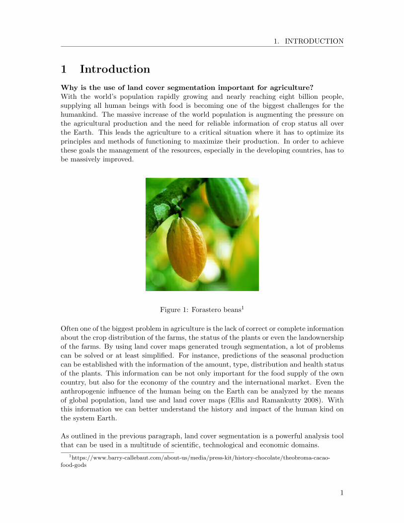
Figure 1: Forastero beans1
Often one of the biggest problem in agriculture is the lack of correct or complete informationabout the crop distribution of the farms, the status of the plants or even the landownershipof the farms. By using land cover maps generated trough segmentation, a lot of problemscan be solved or at least simplified. For instance, predictions of the seasonal productioncan be established with the information of the amount, type, distribution and health statusof the plants. This information can be not only important for the food supply of the owncountry, but also for the economy of the country and the international market. Even theanthropogenic influence of the human being on the Earth can be analyzed by the meansof global population, land use and land cover maps (Ellis and Ramankutty 2008). Withthis information we can better understand the history and impact of the human kind onthe system Earth.
As outlined in the previous paragraph, land cover segmentation is a powerful analysis toolthat can be used in a multitude of scientific, technological and economic domains.
1https://www.barry-callebaut.com/about-us/media/press-kit/history-chocolate/theobroma-cacao-food-gods
1
1. INTRODUCTION
Why is the knowledge of cocoa segmentation important?Cocoa is one of the most economically important crops on Earth. For the majority ofthe producing countries it is one of the critical exports and for the consuming countries akey import. It is typical that the countries with the highest consumption of cocoa do notproduce cocoa themselves, since these country usually do not have appropriate climates forthe production of this sensitive crop.
Cocoa is mostly produced in Africa, Asia and South America. In 2016 the biggest cocoaproducing countries were the Ivory Coast (1, 472, 313 tonnes per year2), Ghana (858, 720tonnes per year2), Indonesia (656, 817 tonnes per year2) and Cameroon (291, 512 tonnesper year2). The two biggest South American producing countries were Brazil (213, 843tonnes per year2) and Ecuador (177, 551 tonnes per year2).
Unlike the more industrialized crops, 80 − 90% of cocoa is still produced in small farms3.Most of the farmers work with outdated farming practices and have limited organizationalinfluence on the market. In the producing countries there are many different practices ofgrowing cocoa and its distribution has rapidly changed in the past decades. The typicalmethod of cocoa farming is the cocoa agroforest where cocoa is planted beside mature tim-ber trees and under giant trees, to provide shades for the crops. In these agroforests cocoais often planted with other varieties of crops as this increases the income security of thefarmers over the whole year. The agroforests arose in a time where the population densitywas low, land and forests abundant, fertilizers unknown and the limiting factors were laborand capital. This method reduces the maintenance work and increases biodiversity, butneeds more land and cocoa is quite slow to mature (Ruf 2011).
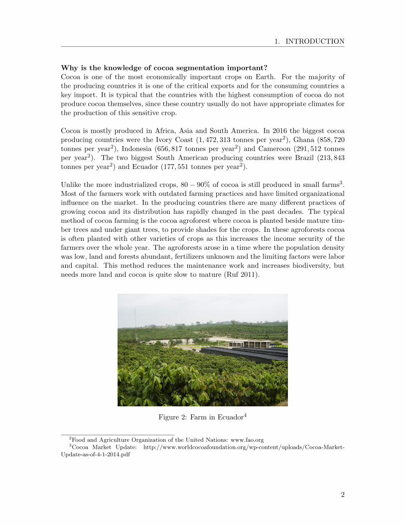
Figure 2: Farm in Ecuador4
2Food and Agriculture Organization of the United Nations: www.fao.org3Cocoa Market Update: http://www.worldcocoafoundation.org/wp-content/uploads/Cocoa-Market-
Update-as-of-4-1-2014.pdf
2
1. INTRODUCTION
As population increased and migration intensified in the last decades, other strategies,such as the full sun farming, became more favored. In full sun cocoa farming, the cocoa isplanted in a single layer structure and hybrid cocoa plants, that can resist the direct sunexposure and give higher yields, are used. In a period of 20 to 25 years, the unshaded andhybrid farms are more profitable than the shaded variant, since their peak yields are earlierand higher (Obiri et al. 2007). Combined with the moderate use of pesticides, fertilizersand herbicides, the abundant yield and return of unshaded cocoa farms can be maintainedfor 25 to 30 years (Ruf 2007). For this method, large areas of forests and agroforests arefelled or burned to win land for new farming. This is called slash-and-burn farming. Thesemethods to acquire land have significantly damaged biodiversity and the forests of themajority of the cocoa-growing countries, such as the Haut-Sassandra forest in Ivory Coast(Barima et al. 2016) and the Bia Conservation Area and Krokosua Hills Forest Reserve inGhana (Asare et al. 2014). Figure 2 shows an example of a full sun cocoa farm in Ecuador.
All these issues around cocoa such as the amount and efficiency of cocoa production, bio-diversity and forest preservation can be observed and analyzed trough cocoa segmentationand cocoa mapping of the affected regions. But not only processes directly linked to cocoaproduction can be distinguished. For instance, also migration and child labor on the farmscan be spotted.
Why do we use satellite images for the task of segmentation?Data collection is a difficult task in most technical and scientific research fields. Beforesatellites and air-based methods were available, the obtainment of the necessary data toproduce a map of a region was an expensive and long lasting undertaking, since the workhad to be manually fulfilled. Satellites provide large amount of data of vast areal extentand high temporal resolution. This quantity of data would not be possible to obtain usingthe typical land surveying methods.
Therefore, plenty of new remote sensing have been developed or refined in the past years.For instance, space-based radar missions, such as Radarsat-2 launched in 2007, light de-tection and ranging (LIDAR) missions, such as ICESat launched in 2003, or multispectralimagery missions, such as Sentinel-2 launched in 2015.
Data collected by satellite is nowadays used in multiple applications. For instance, theobservation of the deforestation of the tropical forest in Central Africa in order to monitorthe change and optimize forest management (Duveiller et al. 2008), the mapping of galam-sey gold mines in Ghana to analyze their relationship with the cocoa agriculture (Snapiret al. 2017) or the mapping crop types to ”provide crucial information for agriculturalmonitoring and management” (Inglada et al. 2016).
4https://www.confectionerynews.com/Article/2015/10/07/Chocolate-firms-eye-Ecuador-for-single-estate-cocoa-Hacienda-Victoria
5https://news.mongabay.com/2016/07/huge-cacao-plantation-in-peru-illegally-developed-on-forest-zoned-land/
3
1. INTRODUCTION
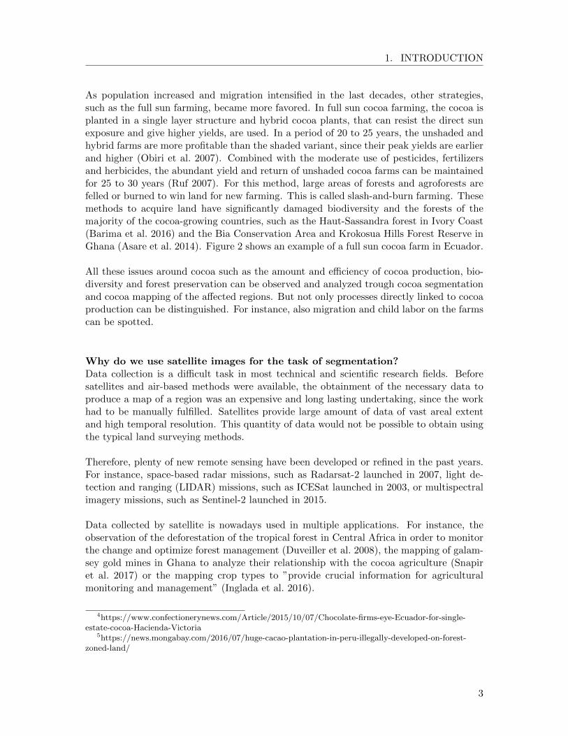
Figure 3: Satellite image of a cocoa farm on forest zone in Peru5
Why do we use deep learning and convolutional neural network for this task?
Deep learning, a type of machine learning techniques, is a family of self-optimization meth-ods that have more than one layer between input and output and, thus, show a complexinner structure. The term deep learning was created by Rina Dechter in 1986 and a multi-tude of varieties have emerged since then such as the multilayer perceptrons (Ivakhnenko1965), backpropagation algorithms, deep neural networks and convolutional deep neuralnetworks (LeCun et al. 1989).
A big revolution in the field of computer vision has been going on since 2012 when itstarted with the introduction of stronger convolutional deep neural networks such as theAlexNet (Krizhevsky et al. 2012) that outperform all the previous classifiers at that time.This evolution has been enhanced by the availability of big, already labeled data sets andpowerful GPU implementations.
Nowadays, convolutional deep neural networks are the front runner for the task of imageclassification as it is a self learning method that combines different features and propertiesof objects and can detect complex topological relations between different items in an image.
The objectives of this Bachelor thesis are:
• Develop a method for cocoa segmentation by combining deep learning methods andsatellite-based multispectral imagery and, thus, improve the feasibility of cocoa seg-mentation.
• Analyze and identify the decisive properties and features of cocoa during the seg-mentation process.
4
2. THEORETICAL PRINCIPLES AND MULTISPECTRAL IMAGES
2 Theoretical Principles and Multispectral Images
2.1 Image Classification
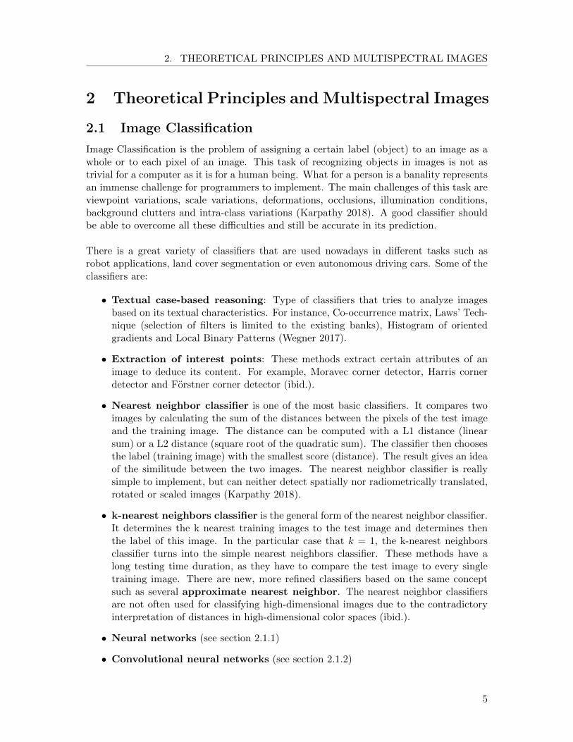
Image Classification is the problem of assigning a certain label (object) to an image as awhole or to each pixel of an image. This task of recognizing objects in images is not astrivial for a computer as it is for a human being. What for a person is a banality representsan immense challenge for programmers to implement. The main challenges of this task areviewpoint variations, scale variations, deformations, occlusions, illumination conditions,background clutters and intra-class variations (Karpathy 2018). A good classifier shouldbe able to overcome all these difficulties and still be accurate in its prediction.
There is a great variety of classifiers that are used nowadays in different tasks such asrobot applications, land cover segmentation or even autonomous driving cars. Some of theclassifiers are:
• Textual case-based reasoning: Type of classifiers that tries to analyze imagesbased on its textual characteristics. For instance, Co-occurrence matrix, Laws’ Tech-nique (selection of filters is limited to the existing banks), Histogram of orientedgradients and Local Binary Patterns (Wegner 2017).
• Extraction of interest points: These methods extract certain attributes of animage to deduce its content. For example, Moravec corner detector, Harris cornerdetector and Forstner corner detector (ibid.).
• Nearest neighbor classifier is one of the most basic classifiers. It compares twoimages by calculating the sum of the distances between the pixels of the test imageand the training image. The distance can be computed with a L1 distance (linearsum) or a L2 distance (square root of the quadratic sum). The classifier then choosesthe label (training image) with the smallest score (distance). The result gives an ideaof the similitude between the two images. The nearest neighbor classifier is reallysimple to implement, but can neither detect spatially nor radiometrically translated,rotated or scaled images (Karpathy 2018).
• k-nearest neighbors classifier is the general form of the nearest neighbor classifier.It determines the k nearest training images to the test image and determines thenthe label of this image. In the particular case that k = 1, the k-nearest neighborsclassifier turns into the simple nearest neighbors classifier. These methods have along testing time duration, as they have to compare the test image to every singletraining image. There are new, more refined classifiers based on the same conceptsuch as several approximate nearest neighbor. The nearest neighbor classifiersare not often used for classifying high-dimensional images due to the contradictoryinterpretation of distances in high-dimensional color spaces (ibid.).
• Neural networks (see section 2.1.1)
• Convolutional neural networks (see section 2.1.2)
5
2. THEORETICAL PRINCIPLES AND MULTISPECTRAL IMAGES
There is no best or universal classifier suited for every task, since each classifier has itsstrengths and weaknesses. For instance, a convolutional neural network is a powerful clas-sifier that once trained is really fast and accurate but needs a considerable amount of dataand time to be correctly trained.
2.1.1 Neural Networks
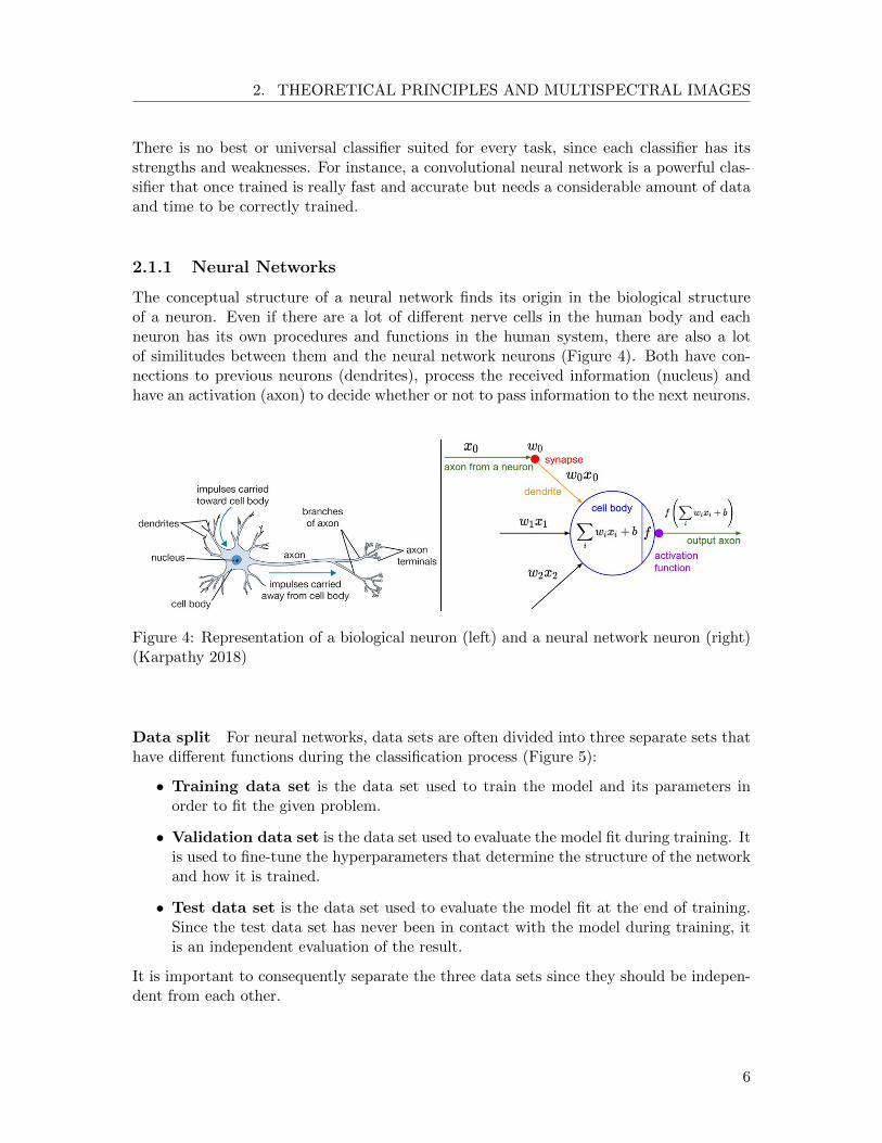
The conceptual structure of a neural network finds its origin in the biological structureof a neuron. Even if there are a lot of different nerve cells in the human body and eachneuron has its own procedures and functions in the human system, there are also a lotof similitudes between them and the neural network neurons (Figure 4). Both have con-nections to previous neurons (dendrites), process the received information (nucleus) andhave an activation (axon) to decide whether or not to pass information to the next neurons.
Figure 4: Representation of a biological neuron (left) and a neural network neuron (right)(Karpathy 2018)
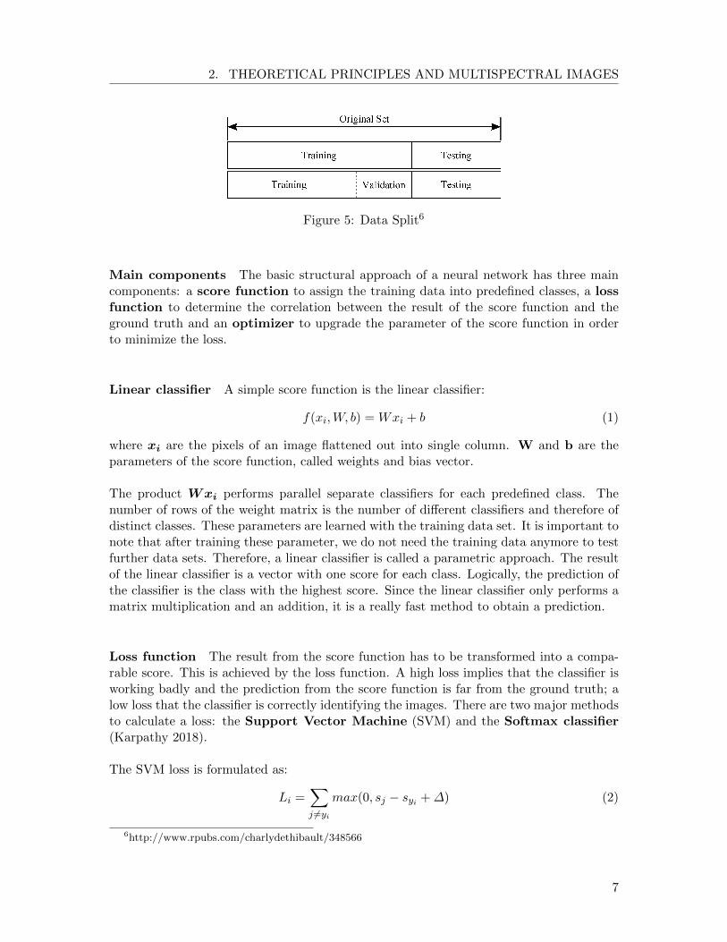
Data split For neural networks, data sets are often divided into three separate sets thathave different functions during the classification process (Figure 5):
• Training data set is the data set used to train the model and its parameters inorder to fit the given problem.
• Validation data set is the data set used to evaluate the model fit during training. Itis used to fine-tune the hyperparameters that determine the structure of the networkand how it is trained.
• Test data set is the data set used to evaluate the model fit at the end of training.Since the test data set has never been in contact with the model during training, itis an independent evaluation of the result.
It is important to consequently separate the three data sets since they should be indepen-dent from each other.
6
2. THEORETICAL PRINCIPLES AND MULTISPECTRAL IMAGES
Figure 5: Data Split6
Main components The basic structural approach of a neural network has three maincomponents: a score function to assign the training data into predefined classes, a lossfunction to determine the correlation between the result of the score function and theground truth and an optimizer to upgrade the parameter of the score function in orderto minimize the loss.
Linear classifier A simple score function is the linear classifier:
f(xi,W, b) = Wxi + b (1)
where xi are the pixels of an image flattened out into single column. W and b are theparameters of the score function, called weights and bias vector.
The product Wxi performs parallel separate classifiers for each predefined class. Thenumber of rows of the weight matrix is the number of different classifiers and therefore ofdistinct classes. These parameters are learned with the training data set. It is important tonote that after training these parameter, we do not need the training data anymore to testfurther data sets. Therefore, a linear classifier is called a parametric approach. The resultof the linear classifier is a vector with one score for each class. Logically, the prediction ofthe classifier is the class with the highest score. Since the linear classifier only performs amatrix multiplication and an addition, it is a really fast method to obtain a prediction.
Loss function The result from the score function has to be transformed into a compa-rable score. This is achieved by the loss function. A high loss implies that the classifier isworking badly and the prediction from the score function is far from the ground truth; alow loss that the classifier is correctly identifying the images. There are two major methodsto calculate a loss: the Support Vector Machine (SVM) and the Softmax classifier(Karpathy 2018).
The SVM loss is formulated as:
Li =∑j 6=yi
max(0, sj − syi +∆) (2)
6http://www.rpubs.com/charlydethibault/348566
7
2. THEORETICAL PRINCIPLES AND MULTISPECTRAL IMAGES
where sj is the class score of the correct class and syi are the class scores of the otherclasses. ∆ is a hyperparameter.
The SVM is a method that seeks the score sj of the correct class to be ∆ higher than thescore syi of the incorrect classes. The max(0,−) function is a threshold function, calledhinge loss. It sets every negative number to zero.
The Softmax classifier corresponds to the cross-entropy of the scores for each class:
Li = − log
(esyi∑j e
sj
)(3)
where syi is the class score of the correct class and∑∑∑
j esj the sum of all the class scores.
The Softmax function takes a vector and squeezes it into a vector with values between zeroand one, that sum up to one. From the point of view of probability theory, the outputcan be seen as a generalized Bernoulli distribution that represents the normalized outcomeprobability for each class.
Whereas the SVM loss directly sets the loss to 0 when the correct score is ∆ higher thanthe score of the incorrect classes, the Softmax classifier also gives an information abouthow much higher the predicted score is from the other ones. For example, the SVM loss(∆ = 1) for [4, 4, 5] and [1, 2, 25] would be the same, however the Softmax loss would not.In practice the SVM loss and the Softmax loss are equally used because there are no bigdivergences between the results of both methods.
Optimization The optimizer tries to find the best possible set of weights W for thegiven classification problem. Due to the fact that this is a nearly impossible task, theoptimizer attempts at each iteration to find a set of new weights W that is just a little bitbetter then the previous one. By starting at a random matrix W and improving it at eachiteration, the optimizer slowly finds a good set of weights W .
Gradient descent is the most common method used to optimize neural networks. The gra-dient descent computes the gradient of the loss function ∇WL(W ) with respect to theparameters W . The loss function L(W ) is then minimized by updating the parametersW in the opposite direction of the gradient. This can be compared to always walkingdownhill until finding the lowest point of a valley.
The learning rate defines the pace at which the parameters are updated at each iteration.This is an important hyperparameter that has to be determined during validation becausea high learning rate can prevent the optimizer to converge on the desired minima. Thelearning rate is often adjusted during training to increase the amount details learned.
There are three different main variants of the gradient descent that vary between the ac-curacy of the computed gradient and the computation time for each update. The batchgradient descent always uses the whole training data set to compute the gradient of
8
2. THEORETICAL PRINCIPLES AND MULTISPECTRAL IMAGES
the loss function. This computes the best possible gradient but is very time consuming.On the contrary, the stochastic gradient descent (SGD) only executes the gradientover a single training example. This method often works well because successive updatesfrequently have the same direction. Compared to the batch gradient descent, the SGD isless accurate, but therefore less time consuming. The mini-batch gradient descent ismidway between the two other methods, as it computes the gradient of small parts of thetraining set, called mini-batches.
Some methods have been developed to optimize the SGD performance in difficult parameterspaces. For instance, the momentum method that, by adding a fraction of the previousupdate to the current update, reduces oscillation in parameter spaces with big slope dif-ferences. This basic idea has been refined in methods such as the Nesterov acceleratedgradient that calculates the current upgrade with an approximation of the parameters ofthe next step.
A recently created optimizer is the Adam optimizer (Kingma and Ba 2014). It is afirst-order gradient-based stochastic optimization combining the advantages of two otherestablished methods: the AdaGrad (Adaptive Gradient Algorithm (Duchi et al. 2011))and the RMSProp (Root Mean Square Propagation). On one side, it adjusts the learningrate during the training (AdaGrad) to perform bigger updates for infrequent and smallerupdates for frequent parameters. On the other side, it also adapts the learning rate (RM-SProp) based on the average magnitude of the recent gradients. The Adam optimizers canbe seen as a heavy ball with friction rolling downhill in the parameter space (Heusel et al.2017).
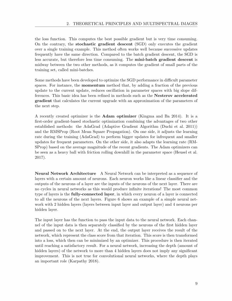
Neural Network Architecture A Neural Network can be interpreted as a sequence oflayers with a certain amount of neurons. Each neuron works like a linear classifier and theoutputs of the neurons of a layer are the inputs of the neurons of the next layer. There areno cycles in neural networks as this would produce infinite iterations! The most commontype of layers is the fully-connected layer, in which every neuron of a layer is connectedto all the neurons of the next layers. Figure 6 shows an example of a simple neural net-work with 2 hidden layers (layers between input layer and output layer) and 4 neurons perhidden layer.
The input layer has the function to pass the input data to the neural network. Each chan-nel of the input data is then separately classified by the neurons of the first hidden layerand passed on to the next layer. At the end, the output layer receives the result of thenetwork, which represent the class score from that iteration. This score is then transformedinto a loss, which then can be minimized by an optimizer. This procedure is then iterateduntil reaching a satisfactory result. For a neural network, increasing the depth (amount ofhidden layers) of the network to more than 4 hidden layers does not imply any significantimprovement. This is not true for convolutional neural networks, where the depth playsan important role (Karpathy 2018).
9
2. THEORETICAL PRINCIPLES AND MULTISPECTRAL IMAGES
Figure 6: Basic neural network architecture (Karpathy 2018)
Data preprocessing Before training, data has to be preprocessed in such way that thedifferent images have approximately the same range and distribution of pixel values. Thisis normally computed in two steps.
First, the mean subtraction is applied to the data in order to achieve a 0 centered dataset. The mean is calculated for each band separately or the whole image and then sub-tracted from the bands or the whole image.
Secondly, the data is compressed between [−1; 1] using the normalization. For this, thedata is divided by the square root over the separate bands or the whole image.
The mean and square root of the data should only be calculated on the training data setand then applied to the training, validation and test data sets. This assures that the 3data sets are still independent from each other and that no information of the test set isused during training. After these two preprocessing steps, the data is standard normallydistributed.
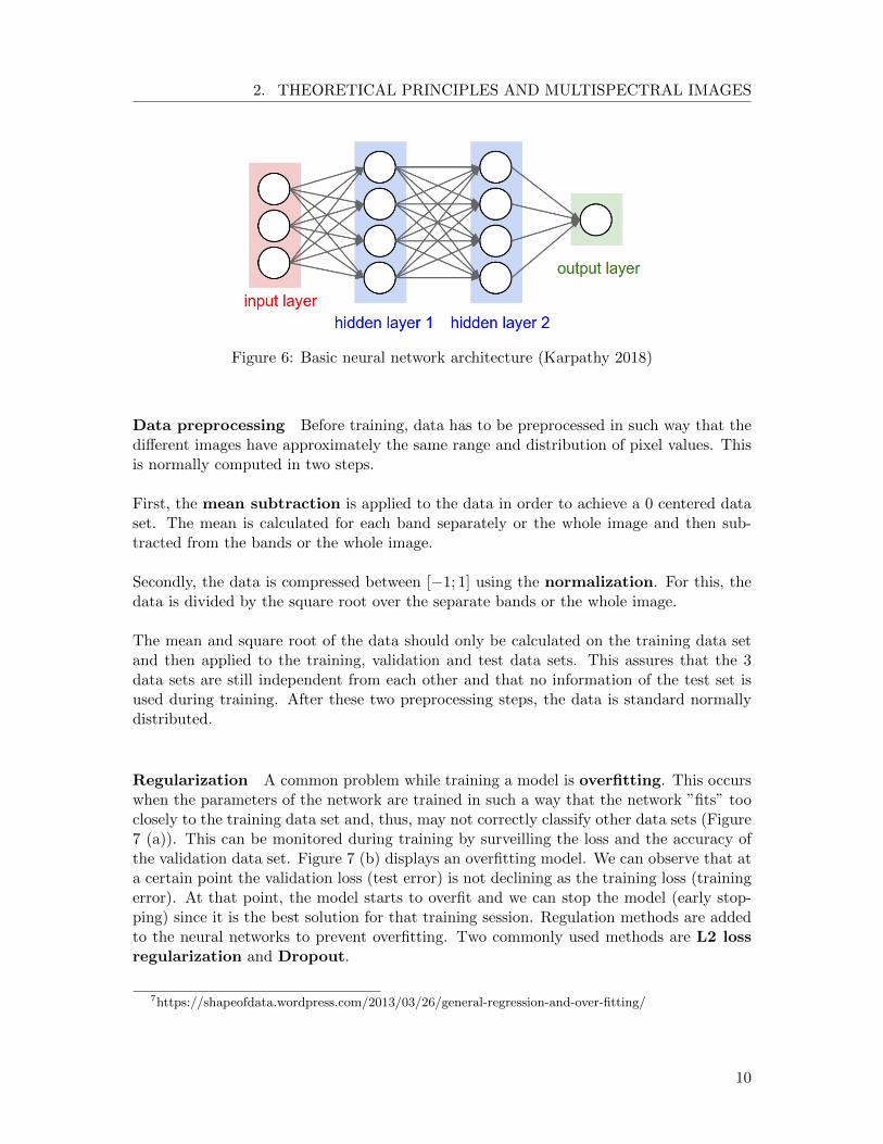
Regularization A common problem while training a model is overfitting. This occurswhen the parameters of the network are trained in such a way that the network ”fits” tooclosely to the training data set and, thus, may not correctly classify other data sets (Figure7 (a)). This can be monitored during training by surveilling the loss and the accuracy ofthe validation data set. Figure 7 (b) displays an overfitting model. We can observe that ata certain point the validation loss (test error) is not declining as the training loss (trainingerror). At that point, the model starts to overfit and we can stop the model (early stop-ping) since it is the best solution for that training session. Regulation methods are addedto the neural networks to prevent overfitting. Two commonly used methods are L2 lossregularization and Dropout.
7https://shapeofdata.wordpress.com/2013/03/26/general-regression-and-over-fitting/
10
2. THEORETICAL PRINCIPLES AND MULTISPECTRAL IMAGES
(a) Example of overfitting (Left: underfitting.Center: good. Right: overfitting)
(b) Monitoring of the loss
Figure 7: Overfitting7
The regularization penalty R(W) is the sum of the L2 norm of the weights from the neuralnetwork:
R(W ) =∑k
∑l
W 2k,l (4)
L = Ldata + λR(W ) (5)
The term R(W) is added to the data loss Ldata (SVM or Softmax) to prevent large weightsin the neural network. These large weights could influence the network not to use all thegiven input data but only a small part of it. λ is a hyperparameter and defines the strengthof the regularization.
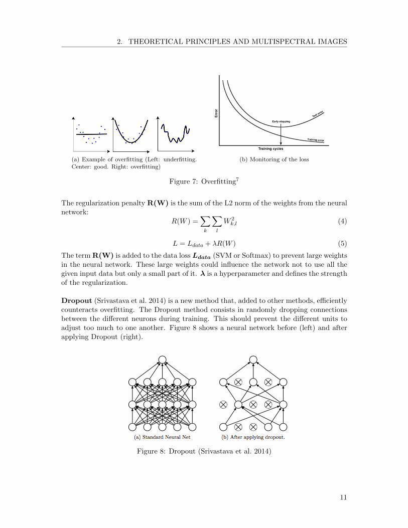
Dropout (Srivastava et al. 2014) is a new method that, added to other methods, efficientlycounteracts overfitting. The Dropout method consists in randomly dropping connectionsbetween the different neurons during training. This should prevent the different units toadjust too much to one another. Figure 8 shows a neural network before (left) and afterapplying Dropout (right).
Figure 8: Dropout (Srivastava et al. 2014)
11
2. THEORETICAL PRINCIPLES AND MULTISPECTRAL IMAGES
2.1.2 Convolutional Neural Networks
Convolutional Neural Networks (CNN) is a class of neural networks used to analyze im-age data. Introduced by LeCun et al. 1989, convolutional neural networks have producedexcellent results in the tasks of classifying handwritten digits and face detection. By us-ing certain characteristics of the images, they reduce the amount of parameters and canthus solve much more complex tasks than other standard classifiers. Since they have morehidden layers (depth) than an ordinary neural network, they need also less preprocessingbecause they can learn it by adjusting its own filters.
There are a lot of similarities between neural networks and convolutional neural networkssuch as the hidden layers, the weighs and biases, the loss function and the optimizer. Themain difference is that convolutional neural networks use a multitude of different layersand have a bigger depth than the neural networks.
The reasons why convolutional neural networks have become so popular in the past fewyears are the availability of big, already labeled data sets, powerful GPU implementationsand new regularization methods such as the dropout method. This recent evolution favorsthe development of convolutional neural networks.
Layers of a convolutional neural network In a convolutional neural networks thereare various types of layers (Karpathy 2018):
• Input Layer is the first layer of the network. As for the neural network (see section2.1.1), it passes the input data to the model.
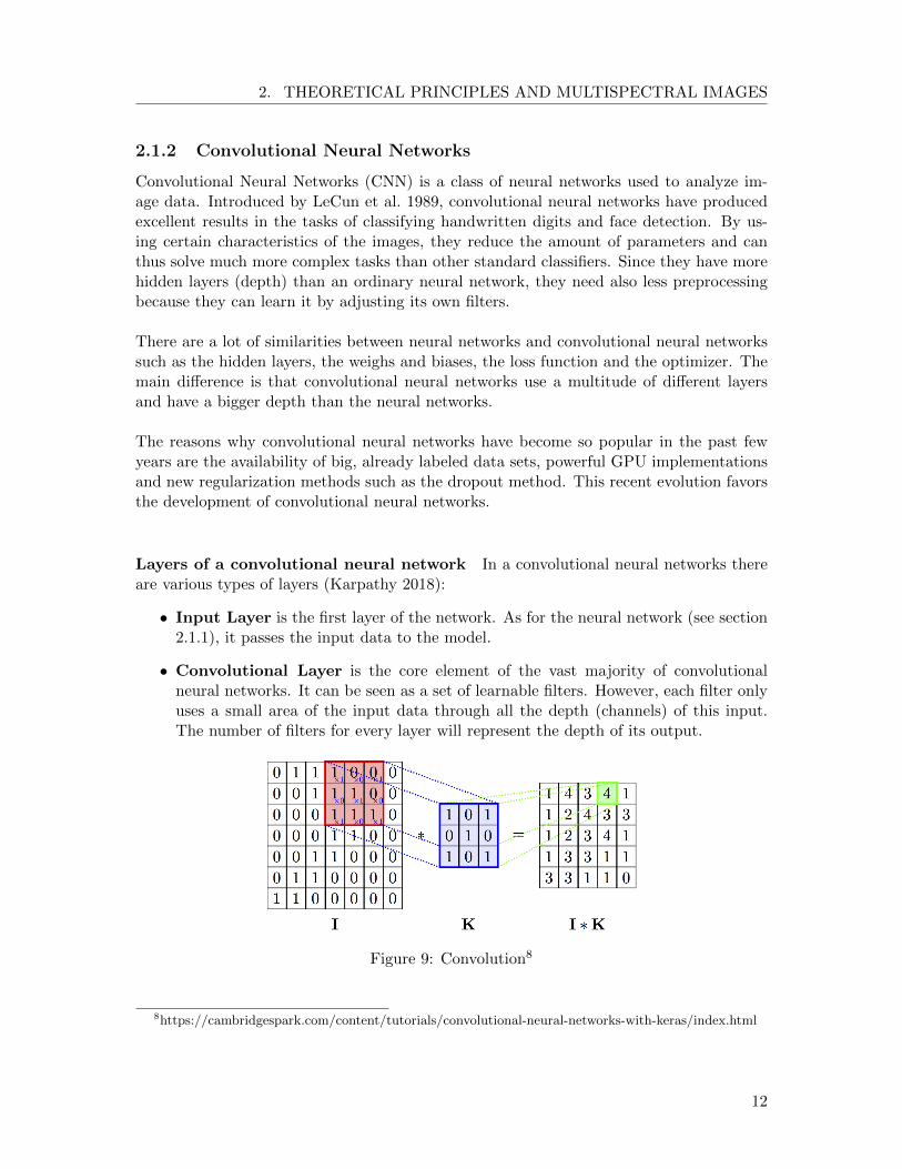
• Convolutional Layer is the core element of the vast majority of convolutionalneural networks. It can be seen as a set of learnable filters. However, each filter onlyuses a small area of the input data through all the depth (channels) of this input.The number of filters for every layer will represent the depth of its output.
Figure 9: Convolution8
8https://cambridgespark.com/content/tutorials/convolutional-neural-networks-with-keras/index.html
12
2. THEORETICAL PRINCIPLES AND MULTISPECTRAL IMAGES
Figure 9 is an example of a convolution with a 3×3 kernel, stride = 1 and padding =0. The stride defines the moving steps of the filter over the image and the paddingthe width of the border zone filled with zeros. The kernel size, stride and paddingare hyperparameters and determine the size of the layer output.
• ReLU Layer: The rectified linear unit is an activation function:
f(x) = max(0, x) (6)
where x is the input of the ReLU layer. This activation function is applied element-wise to the input. By this, the negative values are set to 0. The introduction of ReLUlayer in a model has shown to accelerate the convergence of the stochastic gradientdescent by up to a factor 6 compared to an equivalent model with the activationfunction tanh (Krizhevsky et al. 2012).
Since in certain circumstances it has been observed that a ReLU layer can have theeffect of ”killing” the learning process (by reaching a point where the gradient com-puted by the model is always 0, being equivalent to no learning), more sophisticatedvarieties of this activation layer have been developed. An example is the LeakyReLU where the negative values are not directly set to 0 but are instead set to avery small number to prevent this ”dying effect”.
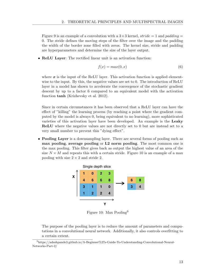
• Pooling Layer is a downsampling layer. There are several forms of pooling such asmax pooling, average pooling or L2 norm pooling. The most common one isthe max pooling. This filter gives back as output the highest value of an area of thesize N ×M and repeats this with a certain stride. Figure 10 is an example of a maxpooling with size 2 × 2 and stride 2.
Figure 10: Max Pooling9
The purpose of the pooling layer is to reduce the amount of parameters and compu-tations in a convolutional neural network. Additionally, it also controls overfitting toa certain extent.
9https://adeshpande3.github.io/A-Beginner%27s-Guide-To-Understanding-Convolutional-Neural-Networks-Part-2/
13
2. THEORETICAL PRINCIPLES AND MULTISPECTRAL IMAGES
• Batch Normalization is often used to increase the stability of neural networks.This layer normalizes the output batch of the previous activation layer. This is im-plemented with a subtraction of the batch mean and a division by the batch standarddeviation. This is comparable with the data preprocessing completed before training.
The batch normalization allows the use of higher learning rates as it directly controlsthe outputs of the different activation layers. It also accelerates the learning processsince the different layers do not have to learn themselves the normalization alreadycomputed by the batch normalization layer. Additionally, it has a small regularizationeffect (Ioffe and Szegedy 2015), sometimes even to the extent of eliminating the needfor dropouts in a model.
• Fully-Connected Layer is the same as in the neural network (see section 2.1.1).
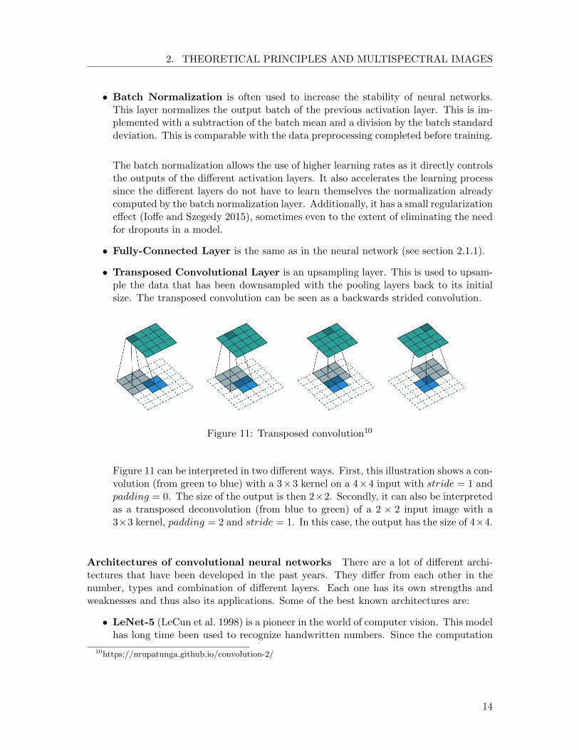
• Transposed Convolutional Layer is an upsampling layer. This is used to upsam-ple the data that has been downsampled with the pooling layers back to its initialsize. The transposed convolution can be seen as a backwards strided convolution.
Figure 11: Transposed convolution10
Figure 11 can be interpreted in two different ways. First, this illustration shows a con-volution (from green to blue) with a 3×3 kernel on a 4×4 input with stride = 1 andpadding = 0. The size of the output is then 2×2. Secondly, it can also be interpretedas a transposed deconvolution (from blue to green) of a 2 × 2 input image with a3×3 kernel, padding = 2 and stride = 1. In this case, the output has the size of 4×4.
Architectures of convolutional neural networks There are a lot of different archi-tectures that have been developed in the past years. They differ from each other in thenumber, types and combination of different layers. Each one has its own strengths andweaknesses and thus also its applications. Some of the best known architectures are:
• LeNet-5 (LeCun et al. 1998) is a pioneer in the world of computer vision. This modelhas long time been used to recognize handwritten numbers. Since the computation
10https://nrupatunga.github.io/convolution-2/
14
2. THEORETICAL PRINCIPLES AND MULTISPECTRAL IMAGES
resources at that time were not as powerful as today, it had a small depth comparedto modern architectures.
• AlexNet (Krizhevsky et al. 2012) outperformed all the previous classifiers in 2012.Having a similar architecture to LeNet-5, it was much deeper using SGD with mo-mentum, dropouts and, for the first time, ReLU activation layers.
• GoogleNet, also called Inception, is an architecture from Google that won theILSVRC 2014 competition. It performs at such a high level that it nearly beatsthe perception performance of a human being. It uses a new element (”Inception”module) based on a lot of small convolutions to reduce the amount of parameters. Asa result, it reduces the number of parameters from 60 million (AlexNet) to 4 million.It also has no fully connected layers.
• ResNet (He et al. 2015) is an 152-layer model and is the winner of the ILSVRC2015 competition. The extreme depth of the ResNet has been a revolution combinedwith the use of residual blocks that merge the output information from before andafter a block build of two convolutional layers. The ResNet model has shown resultsoutperforming the human being.
Data Augmentation The convolutional neural network is a classifier that, once trained,is fast, efficient and thus really powerful, but requires a big amount of training data toacquire good and stable results. Therefore, several techniques, such as data augmentation,have been developed to increase the amount of data when data are scarce. There aredifferent types of data augmentation:
• Translation: The batches can be translated over the original image to create over-lapping batches. This can be done with a fix or a randomly changing stride.
• Rotation: The batches can be rotated to create new batches. This is usually donewith 90, 180 and 270 degrees to quadruple the amount of batches. However, it canalso be computed with finer angles.
• Flipping: The batches can also be flipped on an horizontal or an vertical axis.
• Scaling: The batches can also be created with differently scalings in order to obtainmore and less zoomed batches. This is the same as taking an image of the samescenery from different distances.
• Radiometric Transformations: The batches can also be transformed in radiomet-ric ways by brightening, darkening or changing the contrast of the batches. This canbe compared to taking the same image at different times of a day.
15
2. THEORETICAL PRINCIPLES AND MULTISPECTRAL IMAGES
Unbalanced data Another frequent problem of classifications are unbalanced data sets.These are data sets where the proportion of the different classes in the images are widelydifferent. If this unbalance is too high, it can hinder the convolutional neural network tocorrectly learn, since it will only predict the predominant class without considering theother classes.
This can lead to deceptive results because the accuracy can easily reach values over 90 %only predicting the more frequent class. This phenomenon is called accuracy paradox.Different methods to avoid or minimize the effects of unbalanced data sets are:
• Collecting more data.
• Using other evaluation metrics such as recall, precision and intersection over union(see section 4.1).
• Undersampling is a method that consists in eliminating the batches with solely themajority class. This can help to eliminate redundant data, balance the proportionbetween classes and thus accelerate the processing time and improve the results. Butit must be noted that important information can be lost during this process.
• Higher penalization for errors of the minority class. This is an efficient way toincrease the importance of minority classes during training.
2.2 Multispectral Images
A multispectral image is a superposition of sub-images of the same scenery taken at manydifferent wavelengths. The best known type of multispectral images is the RGB image,composed of a red, a green and a blue sub-image (visible light), each representing a differ-ent wavelength in the electromagnetic spectrum.
The discrete area of the electromagnetic spectrum covered by each sub-image of a multi-spectral image is called a band. The sub-images are then stacked on a third dimensionto one single multispectral image. As a consequence, the multispectral images have thedimension [height of the sub-images, width of the sub-images, number of bands]. While theRGB image only has three bands, there are cameras able to measure a large amount ofbands not only in the visible but also in the non-visible part of the spectrum such as thenear infrared or the short-wavelength infrared. This possibility of extracting informationfrom different spectral bands has shown to be a powerful tool in a big variety of appli-cations. The multispectral images are, for example, used for vegetation segmentation insatellite imagery, for detection of skin diseases or for analyses of art works.
A disadvantage of multispectral images is the increasing need for memory and with thatthe increasing processing time when working with them. However, this will not be a rele-vant problem in the future since the speed, capacity and memory of computers are rapidlyincreasing.
16
2. THEORETICAL PRINCIPLES AND MULTISPECTRAL IMAGES
Further, spectral signatures can be created from multispectral images. These are com-positions of the single values of the electromagnetic energy reflected by a certain object foreach band. Spectral signatures result in distinct curves for every type of object containingthe complete information of the reflectance of this object.
This method is often used in remote sensing to characterize and thus differentiate betweenvarious plants, soil, forest or other items on the earth’s surface. In our case, we assumethat the convolutional neural network will use the information of the spectral signature ofthe different objects to segment the images between them.
2.2.1 Sentinel-2
Sentinel is one of the latest Earth observation missions from ESA. This project has replacedolder ESA-missions, which reached or are reaching their respective retirement dates, suchas the ERS missions (1991 - 2011). The Sentinel satellites are equipped with a wide rangeof technologies, such as radars or multispectral imaging instruments used for land, oceanand atmospheric monitoring. There are five different Sentinel missions, each focusing ondifferent aspects of Earth observation. Each mission has a constellation of two satellites toprovide a periodic coverage of observation data of the whole Earth11:
• Sentinel-1: land and ocean monitoring using radar imaging
• Sentinel-2: land monitoring focusing on vegetation, soil and coastal areas usinghigh-resolution optical multispectral imagery
• Sentinel-3: marine observation
• Sentinel-4 and Sentinel-5: air quality monitoring
General Information Sentinel-2 is a high-resolution, multispectral imaging missionforming part of the Copernicus Programme, the largest Earth observation programme.The Sentinel-2 system is composed of two satellites. The S2A satellite was launched onthe 23th of June 2015 and S2B on the 7th March 2017. Both satellites have an operationlifespan of approximately 7.5 years. The constellation of two sun-synchronous satellitesflying in the same orbit with an altitude of 786 km and an inclination of 98.62◦ enables thepossibility of monitoring the Earth with a frequency of five days and to always maintain thesame angle of sunlight on the Earth’s surface. These properties are useful for the creationof a consistent time series data collection.
11https://sentinel.esa.int/web/sentinel/home12https://earth.esa.int/web/sentinel/user-guides/sentinel-2-msi/resolutions/spatial
17
2. THEORETICAL PRINCIPLES AND MULTISPECTRAL IMAGES
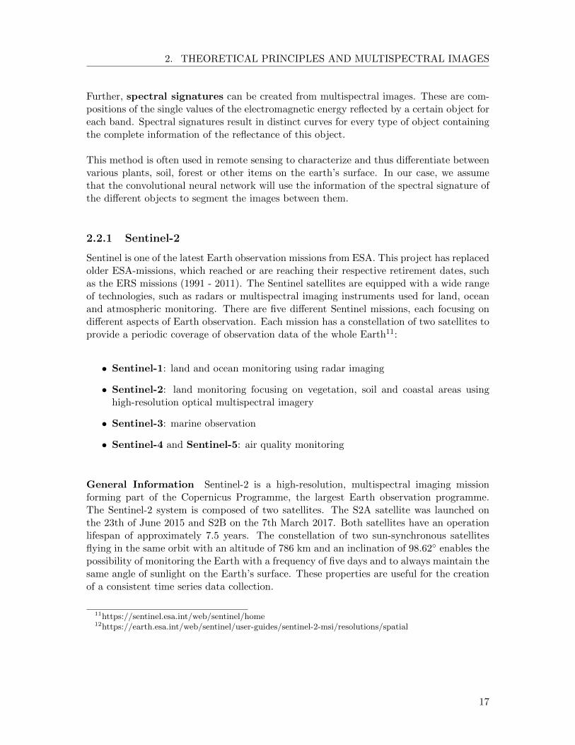
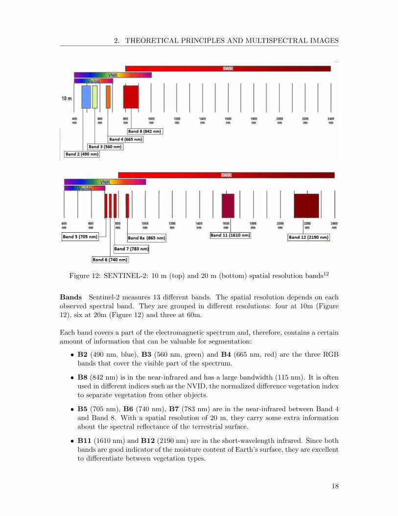
Figure 12: SENTINEL-2: 10 m (top) and 20 m (bottom) spatial resolution bands12
Bands Sentinel-2 measures 13 different bands. The spatial resolution depends on eachobserved spectral band. They are grouped in different resolutions: four at 10m (Figure12), six at 20m (Figure 12) and three at 60m.
Each band covers a part of the electromagnetic spectrum and, therefore, contains a certainamount of information that can be valuable for segmentation:
• B2 (490 nm, blue), B3 (560 nm, green) and B4 (665 nm, red) are the three RGBbands that cover the visible part of the spectrum.
• B8 (842 nm) is in the near-infrared and has a large bandwidth (115 nm). It is oftenused in different indices such as the NVID, the normalized difference vegetation indexto separate vegetation from other objects.
• B5 (705 nm), B6 (740 nm), B7 (783 nm) are in the near-infrared between Band 4and Band 8. With a spatial resolution of 20 m, they carry some extra informationabout the spectral reflectance of the terrestrial surface.
• B11 (1610 nm) and B12 (2190 nm) are in the short-wavelength infrared. Since bothbands are good indicator of the moisture content of Earth’s surface, they are excellentto differentiate between vegetation types.
18
2. THEORETICAL PRINCIPLES AND MULTISPECTRAL IMAGES
The bands with a 60 m spatial resolution are used to measure the atmospheric conditionsneeded during the preprocessing of the images.
Product types The data measured by the Sentinel-2 satellites have to be preprocessedbefore being ready for applications. There are different product types corresponding to thedifferent stages of this preprocessing13:
• Level-1B: The Level-1B product type contains the information of the top-of-atmosphereradiance values in sensor geometry. It also includes geometric information needed togenerate the Level-1C product type
• Level-1C The Level-1C product type are 100x100km2 tiles containing the top-of-atmosphere reflectance in cartographic geometry (ortho-images in UTM/WGS84 pro-jection). This product is generated using a Digital Elevation Model to project theimagery.
• Level-2A The Level-2A product type are bottom-of-atmosphere reflectance imagesin cartographic geometry. They are also 100x100km2 in UTM/WGS84 projection.At this moment, ESA is only generating this product type for images of the Europeancontinent. The Level-2A product type can be individually created by the users fromthe Level-1C product type using the ”Sentinel-2 Toolbox”, called SNAP (SentinelApplication Platform).
13https://sentinel.esa.int/web/sentinel/user-guides/sentinel-2-msi/product-types
19

3. METHODOLOGY
3 Methodology
In this section, we will illustrate the cocoa segmentation method developed for this project.For this purpose, we will individually introduce each component of the method and explaintheir importance, functioning and effect on the final results. Additionally, we will outlinesome methods in order to better understand the learning process and identify the decisivefeatures during cocoa segmentation.
Considering that cocoa is planted with different techniques (section 1), we will distinguishbetween full sun farming and agroforestry by using Ecuadorian farms as a model for thefull sun farms and Ghanian farms for the agroforestry.
3.1 Convolutional Neural Network
For the task of cocoa segmentation, we need a convolutional neural network that performsa semantic segmentation, which is a classification at pixel-level. As opposite to classifyingthe whole image to one label, semantic segmentation is necessary for this project becausewe not only want to determine the presence of cocoa in the analyzed area but also itsdistribution and the total amount.
The program developed in this project is implemented on TensorFlow, an open-sourcesoftware library for dataflow programming based on Python and developed by the GoogleBrain team.
3.1.1 Architecture: U-Net
We choose an architecture based on U-Net (Ronneberger et al. 2015), a popular semanticsegmentation model. The U-Net model is an encoder-decoder architecture where the inputdata are downsampled to a lower spatial dimension and then upsampled back to its initialspatial resolution to allow a pixelwise classification. This architecture has shown goodresults with small data sets and strong use of data augmentation methods.
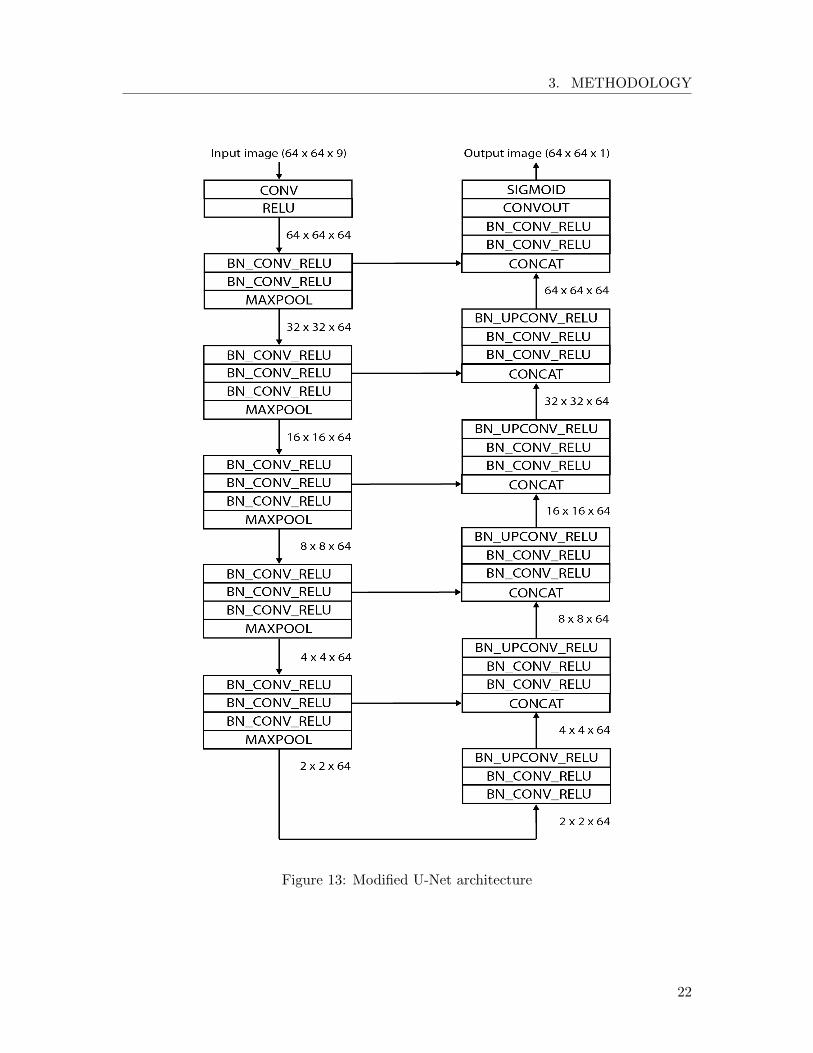
The modified U-Net architecture (Nowaczynski et al. 2017) used for this project is onlybuild of convolutional, transposed convolutional, ReLU, batch normalization and maxpoollayers (see section 2.1.2). There are no fully-connected layers in this architecture, sincethe upsampling part is achieved using only transposed convolutional layers. The structureof the model can be seen in Figure 13. The main differences between the original U-Netarchitecture and our modified U-Net model are changes in the input image dimensions andvarious hyperparameters of layers, for instance the number of kernels per convolutionallayer.
The architecture is mainly build of BN CONV RELU and BN UPCONV RELU blocks(Figure 13). The BN CONV RELU block is used during the whole model and is composed
21
3. METHODOLOGY
Figure 13: Modified U-Net architecture
22
3. METHODOLOGY
of:
• a batch normalization layer,
• a convolutional layer with 64 kernels of size = 3 × 3, stride = 1 and padding = 1,
• a ReLU layer (activation function).
The BN UPCONV RELU block is only used during the upsampling phase (right side ofthe model) and is composed of:
• a batch normalization layer,
• a transposed convolutional layer with 64 kernels of size = 3 × 3, stride = 2 andpadding = 1,
• a ReLU layer (activation function).
The U-form of the architecture stands for the downsampling (left side) and upsamplingphases (right side) of the model (Figure 13). The downsampling is achieved with five max-pooling layers with kernel size = 2 × 2, stride = 2 and padding = 0. As a result of thehyperparameter choice of the pooling layer, the output size (height and width) of theselayers is always half of the input size. On the other side of the model, transposed convo-lutional layers are used to upsample the data back to its initial size in order to be able todetermine the label for every pixel of the input batch.
It is important to note that, during the upsampling phase, the output of the transposedconvolutional layer is consistently concatenated with the same size data from the down-sampling phase. This can be observed in Figure 13 pictured by horizontal arrows and thebox CONCAT. The concatenation is executed on the third dimension. This allows themodel to combine the more detailed information from the downsampling phase with themuch more generalized information of the upsampling phase.
The CONVOUT layer is a convolutional layer with 2 kernels of size = 1 × 1, stride = 1and padding = 0 followed by a sigmoid function (activation function). The output ofthe U-Net model is a vector with the class score between 0 and 1 of each pixel (”NoCocoa”= 0/”Cocoa”= 1).
3.1.2 Training Details
The model is trained with multispectral images from the Sentinel-2 satellites. The classscore vector resulting from the U-Net architecture is then transformed into a loss scoreusing a Softmax cross-entropy function. The L2 loss of the weights is then added to thecross-entropy loss in order to prevent overfitting (Regularization). The model is trainedusing an Adam optimizer minimizing the total loss.
The hyperparameters of our network and their corresponding default values are:
23
3. METHODOLOGY
• Number of training epochs is adjusted in respect to the amount of batches of theinput data set for the respective training session.
• Learning rate is set to a standard value of 10−5.
• L2 regularization is set to a standard value of 10−2.
• Mini-batch size is the number of batches trained at once and thus used to computethe training updates. This parameter is set to 32.
3.2 Ground Truth and Data Split
One of the most important components when performing a good classification is to have anaccurate and complete ground truth of the analyzed area. The information of the sceneryis often difficult to acquire since it mostly has to be manually assembled. As a consequence,this part of the project data is usually the most incomplete and inaccurate part of the in-formation used during segmentations. This problem also affects our project and has beencarefully handled.
In order to minimize the probability of incorrect labeling and, by that, of interfering withthe learning process of the convolutional neural network, the images are labeled in threedifferent classes:
• Cocoa
• Background
• Uncertain
This partition using a third class should prevent to falsely label cocoa pixels with the la-bel ”background”. It is important to note that the pixels labeled as ”uncertain” will notbe used during training, since these would completely confuse the learning process of thenetwork.
Since data are sparse in our project, we decided to split our data set in only two indepen-dent data sets: a training data set and a validation data set. The validation data set willnot only be used for the fine-tuning of the hyperparameters but also for the final test. Thevalidation data set will be independent enough to be a good reference for our experimentssince it will just have been sparsely in contact with the model before the final test.
3.2.1 Ecuador
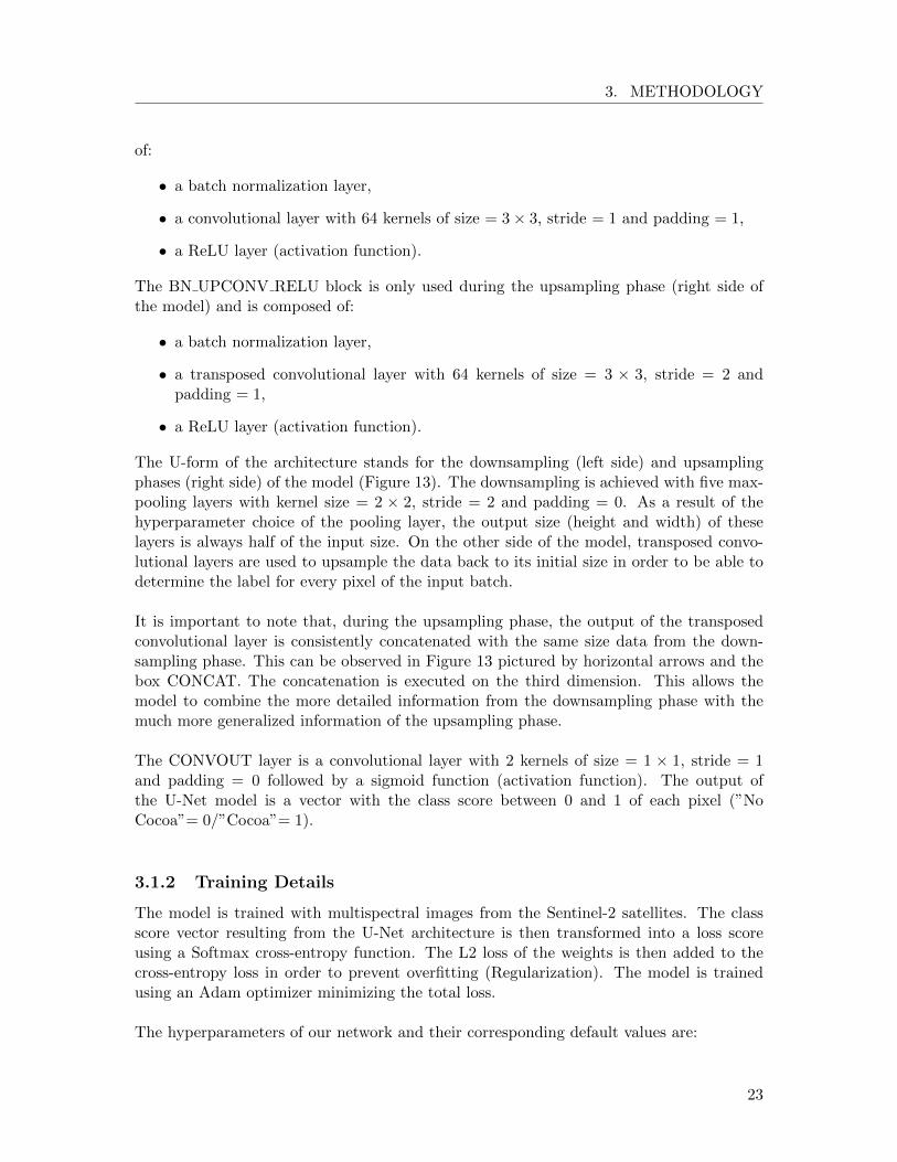
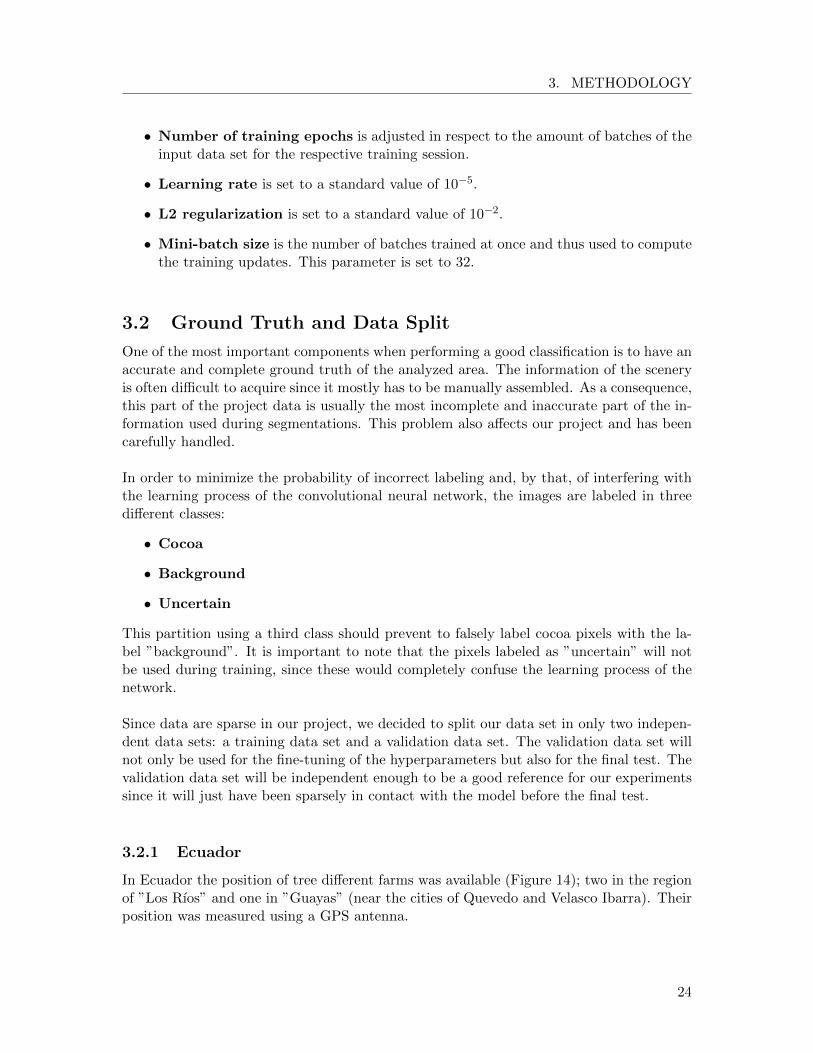
In Ecuador the position of tree different farms was available (Figure 14); two in the regionof ”Los Rıos” and one in ”Guayas” (near the cities of Quevedo and Velasco Ibarra). Theirposition was measured using a GPS antenna.
24
3. METHODOLOGY
Figure 14: Farms in Ecuador
We used Google Earth images to locate and map the farms, since the GPS points justindicated the position of the farm entrances. This mapping task is doable since in Ecuadorcocoa is mostly planted in full sun farms, easy to recognize on satellite imagery. Unfor-tunately, all the Google Earth orthophotos from the area of the farm in ”Guayas” wereblurred. Therefore, it was impossible to correctly identify and, thus, map the farm. Wedecided to use only the other two farms in the region of ”Los Rıos”, which are next to eachother. Since the orthophotos of that region were very clear, we could easily locate, mapand create shape-files of the ground truth of both farms. The first farm has an area of 150hectares and the second one an area of 125.
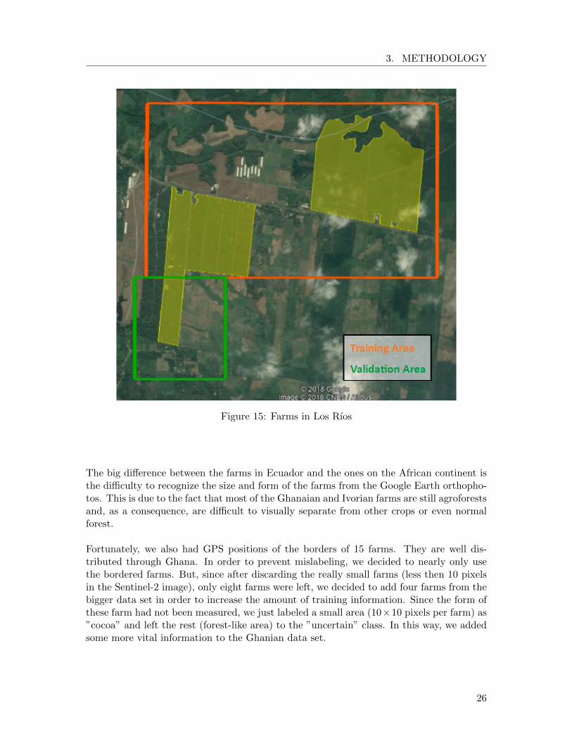
To correctly train the farms in Ecuador, we divided the area of the two selected farms intotwo spatially separated areas, a big ”Training Area” and a smaller ”Validation Area”. Thissubdivision is shown in Figure 15.
3.2.2 Ghana
In Ghana and Ivory Coast, we have a data set of approximately 175 farms, that have beenmapped between April 2016 and December 2017. These farms are well distributed overboth countries, mostly between the latitudes of 5◦N and 7◦N, and cover the regions ofEastern (GH), Ashanti (GH), Western (GH), Comoe (CI), Lagunes (CI), Bas-Sassandra(CI), Sassandra-Marahoue (CI) and Montagnes (CI). As for the farms in Ecuador, theposition of the farms was measured with a GPS-antenna.
25
3. METHODOLOGY
Figure 15: Farms in Los Rıos
The big difference between the farms in Ecuador and the ones on the African continent isthe difficulty to recognize the size and form of the farms from the Google Earth orthopho-tos. This is due to the fact that most of the Ghanaian and Ivorian farms are still agroforestsand, as a consequence, are difficult to visually separate from other crops or even normalforest.
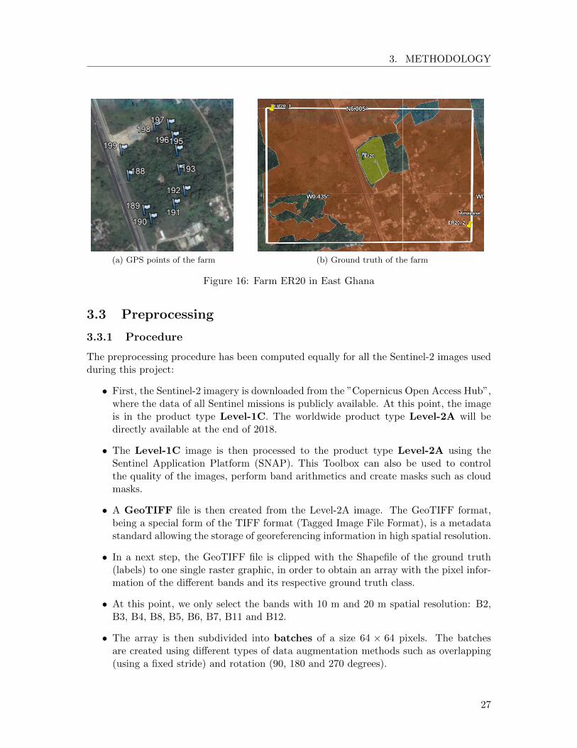
Fortunately, we also had GPS positions of the borders of 15 farms. They are well dis-tributed through Ghana. In order to prevent mislabeling, we decided to nearly only usethe bordered farms. But, since after discarding the really small farms (less then 10 pixelsin the Sentinel-2 image), only eight farms were left, we decided to add four farms from thebigger data set in order to increase the amount of training information. Since the form ofthese farm had not been measured, we just labeled a small area (10×10 pixels per farm) as”cocoa” and left the rest (forest-like area) to the ”uncertain” class. In this way, we addedsome more vital information to the Ghanian data set.
26
3. METHODOLOGY
(a) GPS points of the farm (b) Ground truth of the farm
Figure 16: Farm ER20 in East Ghana
3.3 Preprocessing
3.3.1 Procedure
The preprocessing procedure has been computed equally for all the Sentinel-2 images usedduring this project:
• First, the Sentinel-2 imagery is downloaded from the ”Copernicus Open Access Hub”,where the data of all Sentinel missions is publicly available. At this point, the imageis in the product type Level-1C. The worldwide product type Level-2A will bedirectly available at the end of 2018.
• The Level-1C image is then processed to the product type Level-2A using theSentinel Application Platform (SNAP). This Toolbox can also be used to controlthe quality of the images, perform band arithmetics and create masks such as cloudmasks.
• A GeoTIFF file is then created from the Level-2A image. The GeoTIFF format,being a special form of the TIFF format (Tagged Image File Format), is a metadatastandard allowing the storage of georeferencing information in high spatial resolution.
• In a next step, the GeoTIFF file is clipped with the Shapefile of the ground truth(labels) to one single raster graphic, in order to obtain an array with the pixel infor-mation of the different bands and its respective ground truth class.
• At this point, we only select the bands with 10 m and 20 m spatial resolution: B2,B3, B4, B8, B5, B6, B7, B11 and B12.
• The array is then subdivided into batches of a size 64 × 64 pixels. The batchesare created using different types of data augmentation methods such as overlapping(using a fixed stride) and rotation (90, 180 and 270 degrees).
27
3. METHODOLOGY
• Mean subtraction and normalization are applied to these batches. The mean and thestandard deviation are calculated separately for every band of the training data setand is then applying to the entire data set.
3.3.2 Selection of the Imagery
The images used for this project have been chosen considering the coverage area of theimage, the main crop season (September - February) and the percentage of cloud coverwhen the data was acquired:
• Ecuador: We used imagery of the position MPU (Sentinel-2 code for the differentmeasurement positions) that covers the lower center part of the country
– 8th of November 2017: cloud coverage of 31.02%
• Ghana The Ghanian observation area, being larger than the one in Ecuador, isdistributed over four different Sentinel-2 images with the positions NWM, NXN,NYM and NYN. Additionally, we choose four different imagery dates to increase theamount of image data and have the possibility to use the temporal information ofthe cocoa growth.
– 23th of December 2017: cloud coverage between 28.85% and 84.17%
– 2nd of January 2018: cloud coverage between 0.00 % and 20.19%
– 12th of January 2018: cloud coverage between 5.81% and 14.62%
– 27th of January 2018: cloud coverage of 0.00%
3.4 Analysis of the Learning Process
As mentioned earlier, convolutional neural networks are powerful classifiers that achievehigh accuracies in many different tasks. However, it is still difficult to determine which arethe factors and properties of the multispectral images that a convolutional neural networkuses to recognize and segment cocoa. In this section, we will analyze some components ofthe convolutional neural networks and multispectral images in order to better understandwhich aspects of the cocoa crop influence the classifier.
3.4.1 Importance of the Different Bands
In this section, we will determine which bands of the Sentinel-2 multispectral images havepivotal information for the segmentation process. Therefore, we will test different combi-nations of bands and compare the test results of the different trainings:
• RGB Bands (B2, B3 and B4): This is equivalent to taking an image with a normalthree band camera. If this combination reaches comparable results, then we will beable to say that the use of multispectral images is unnecessary for this task.
28
3. METHODOLOGY
• Dropping each band separately: This will reveal if one of the nine bands isindispensable for cocoa segmentation.
• NDVI Band (B4 and B8): The normalized difference vegetation index is a well-known index often used for vegetation segmentation.
• RGB-NIR Bands (B2, B3, B4 and B8): Combined RGB and near infrared camerasare nowadays a popular tool for image segmentation.
Beside these combinations, we will also further analyze bands that have shown some sig-nificant relevance during these experiments.
3.4.2 Spectral Signature of Cocoa
As outlined in section 2.2, spectral signatures are often used to differentiate between differ-ent surface objects and show clear visible differences between various plant types. There-fore, we will analyze the spectral signature of cocoa and nearby elements such as forest orother plants. Further, we will investigate the different correlations between these objectsand their spectral signature.
• In Ecuador, we will compute the spectral signature of cocoa, forest, bare soil and aneighbor crop field.
• In Ghana, we will compute the spectral signature of cocoa from two different farmsfor three different dates.
• Last, we will compare the spectral signatures of cocoa between Ecuador and Ghana.Additionally, we will also compute the spectral signature of two Ghanian forests(Mamiri Forest Reserve and Boin Tano Forest Reserve) in order to obverse the dif-ference between tropical forests and agroforests.
These three analyses will give us information about the distinctness between cocoa and itsnearby areas, the evolution of the cocoa crop and the difference between cocoa in full sunfarming (Ecuador) and in agroforests (Ghana).
To compute the spectral signature of an object, we will cut out a certain area covered bythat object and calculate the mean value for each band reflectance values separately. Thisresults in one mean value per band. For the spectral signature of cocoa in Ghana (thirdanalysis), we will additionally average the reflectance values over the three data acquisitiondates.
3.5 Cocoa Segmentation in Ghana
Since the situation in Ghana with the agroforests farming and the small amount of suitableinformation is particularly difficult, we approach this issue separately in this section.
29
3. METHODOLOGY
The data set used to train the Ghanian farms is sparse (12 small farms) and really unbal-anced (proportion between cocoa and the rest of the image is smaller then 1/30). Thesetwo factors, also being present in the Ecuadorian data set, are more extreme in the Gha-nian data set. The sparsity and imbalance of data are two big problems while traininga convolutional neural network because the model is fed with a very small amount of in-complete information. We will try to use different techniques to counteract these two issues.
3.5.1 Temporal Data
The first method used to deal with the problem of the limited quantity of data is the use ofmultispectral images from different dates. These temporal data give to the network extrainformation about the growth process not only of the cocoa crop but also of the otherplants surrounding them, such as shading trees.
Therefore, as mentioned in section 3.3.2, we selected Sentinel-2 images from four differentdays in December 2017 and January 2018. The multispectral images of the same area arethen stacked over one another on the band dimension, in order to obtain an input image ofthe size 64 × 64 × 36. This change of the input dimensions does not alter the architecture(see section 3.1.1) or the hyperparameters, still set to the standard parameters defined insection 3.1.2. By following this method, we will have multispectral images of certain areaswith the information of the development of the farms during December and January.
3.5.2 Unbalanced Data Set
Methods that artificially create, select and delete information of the original data set inorder to diminish the imbalance between classes are:
Data augmentation A method described in section 2.1.2 to increase the amount ofdata in a data set is data augmentation. For this project, we only used the translation androtation methods. We implemented the translation by creating overlapping 64 × 64-pixelbatches from the original multispectral images. Then, these batches are rotated by 90, 180and 270 degrees to quadruple the amount of batches. These two augmentation methodshave been applied not only on the Ghanian but also on the Ecuadorian data set.
We did not use scaling as a data augmentation method since the Sentinel-2 imagery is al-ways taken from the same satellite altitude and this would have created useless informationfor the convolutional neural network.
Undersampling We used the method of undersampling in different degrees to comparethe effects of this technique. Undersampling consists in setting a minimum amount of cocoaper batch and thus eliminates the batches with a lower amount of cocoa. As a consequence,
30
3. METHODOLOGY
the proportion between cocoa, background and uncertainty in the data set will prominentlyshift toward cocoa.
We tested different values of the minimal amount of cocoa per batch. For the batch ofsize 64 × 64, we computed the undersampling for the values 100 and 200, representing aminimum of 2.5% and 5% of cocoa per batch.
Batch size Another possibility to counteract the imbalance of our Ghanian data set isto reduce the batch size (height and width) from 64 to 32. This reduction will decrease thearea covered by a batch by four and thus, combined with selective undersampling, createa multitude of batches with a higher percentage of cocoa.
This method will also reduce the amount of information of the surrounding of the farm fedto the convolutional neural network. Consequently, the results will give us an indicationabout the importance of the environment of the farms for cocoa segmentation.
31

4. RESULTS AND DISCUSSION
4 Results and Discussion
4.1 Evaluation
The most common way of evaluating the results of a binary classification problem is theuse of the concepts of Recall, Precision, Accuracy and Intersection over Union. These fourauxiliary variables visualize the correctness of our predictions. To define them, we need tointroduce first the notions of ”True Positive”, ”True Negative”, ”False Positive” and ”FalseNegative”.
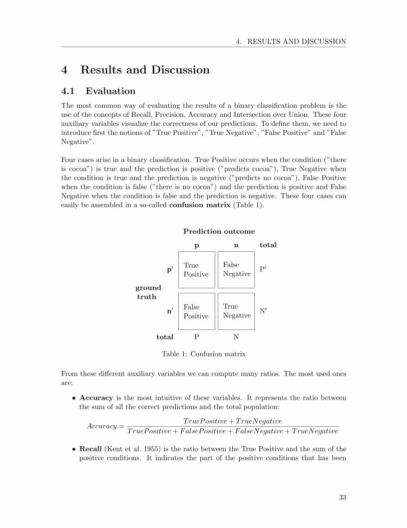
Four cases arise in a binary classification. True Positive occurs when the condition (”thereis cocoa”) is true and the prediction is positive (”predicts cocoa”), True Negative whenthe condition is true and the prediction is negative (”predicts no cocoa”), False Positivewhen the condition is false (”there is no cocoa”) and the prediction is positive and FalseNegative when the condition is false and the prediction is negative. These four cases caneasily be assembled in a so-called confusion matrix (Table 1).
groundtruth
Prediction outcome
p n total
p′TruePositive
FalseNegative
P′
n′FalsePositive
TrueNegative
N′
total P N
Table 1: Confusion matrix
From these different auxiliary variables we can compute many ratios. The most used onesare:
• Accuracy is the most intuitive of these variables. It represents the ratio betweenthe sum of all the correct predictions and the total population:
Accuracy =TruePositive+ TrueNegative
TruePositive+ FalsePositive+ FalseNegative+ TrueNegative
• Recall (Kent et al. 1955) is the ratio between the True Positive and the sum of thepositive conditions. It indicates the part of the positive conditions that has been
33
4. RESULTS AND DISCUSSION
correctly predicted:
Recall =TruePositive
TruePositive+ FalseNegative
• Precision (Kent et al. 1955) is the ratio between the True Positive and the sum ofthe positive predictions. It characterizes the predictions that are correct and thusactually useful:
Precision =TruePositive
TruePositive+ FalsePositive
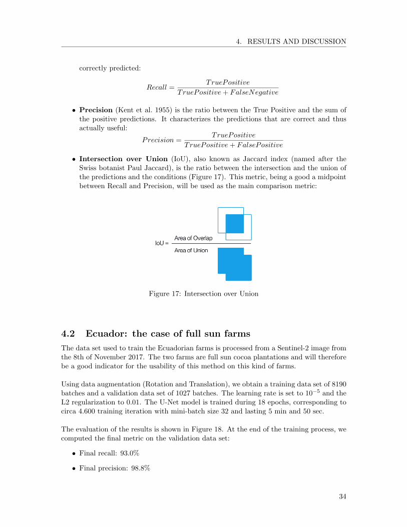
• Intersection over Union (IoU), also known as Jaccard index (named after theSwiss botanist Paul Jaccard), is the ratio between the intersection and the union ofthe predictions and the conditions (Figure 17). This metric, being a good a midpointbetween Recall and Precision, will be used as the main comparison metric:
Figure 17: Intersection over Union
4.2 Ecuador: the case of full sun farms
The data set used to train the Ecuadorian farms is processed from a Sentinel-2 image fromthe 8th of November 2017. The two farms are full sun cocoa plantations and will thereforebe a good indicator for the usability of this method on this kind of farms.
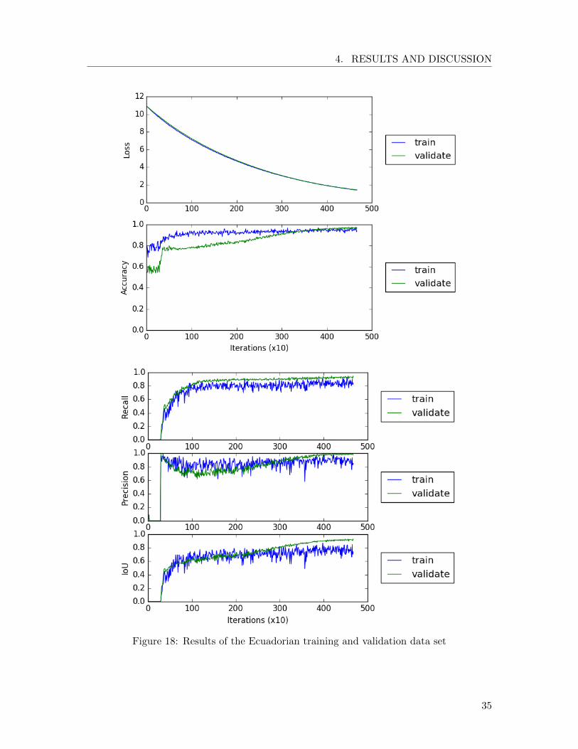
Using data augmentation (Rotation and Translation), we obtain a training data set of 8190batches and a validation data set of 1027 batches. The learning rate is set to 10−5 and theL2 regularization to 0.01. The U-Net model is trained during 18 epochs, corresponding tocirca 4.600 training iteration with mini-batch size 32 and lasting 5 min and 50 sec.
The evaluation of the results is shown in Figure 18. At the end of the training process, wecomputed the final metric on the validation data set:
• Final recall: 93.0%
• Final precision: 98.8%
34
4. RESULTS AND DISCUSSION
Figure 18: Results of the Ecuadorian training and validation data set
35
4. RESULTS AND DISCUSSION
• Final intersection over union: 92.0%
These are impressive results considering the limited amount of training data. We noticethat the precision of the predictions is nearly 100%. This means that the convolutionalneural network rarely assigns cocoa to a pixel labeled as background in the ground truth.This error is known as false positive error or type I error.
When examining the loss and accuracy curves (Figure 18 (a)), no signs of overfitting canbe observed since the training and the validation curves nicely converge to the same valuesand no significant drifting apart occurs. On the intersection over union curve, we can seethat the intersection over union of the validation reaches a much higher value than thetraining. This is probably due to fact that the training area (Figure 15) contains morecomplex shapes and a higher diversity of plants.
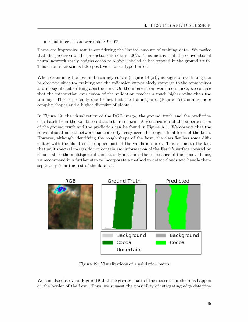
In Figure 19, the visualization of the RGB image, the ground truth and the predictionof a batch from the validation data set are shown. A visualization of the superpositionof the ground truth and the prediction can be found in Figure A.1. We observe that theconvolutional neural network has correctly recognized the longitudinal form of the farm.However, although identifying the rough shape of the farm, the classifier has some diffi-culties with the cloud on the upper part of the validation area. This is due to the factthat multispectral images do not contain any information of the Earth’s surface covered byclouds, since the multispectral camera only measures the reflectance of the cloud. Hence,we recommend in a further step to incorporate a method to detect clouds and handle themseparately from the rest of the data set.
Figure 19: Visualizations of a validation batch
We can also observe in Figure 19 that the greatest part of the incorrect predictions happenon the border of the farm. Thus, we suggest the possibility of integrating edge detection
36
4. RESULTS AND DISCUSSION
methods to improve the results on the transitions between ”cocoa” and ”background”.
Furthermore, it is important to note that the results of this section are the training out-come of a data set with only two, very similar farms. Therefore, these results have tobe validated with a larger data set containing more farms distributed trough the wholecountry before being able to confirm the viability of this method on all full sun farms.
4.3 Analysis of the Learning Process
In this section we will analyze which aspects and properties of the convolutional neuralnetwork and the multispectral images are decisive during the process of cocoa segmenta-tion. This will give us a better understanding of the learning process and, thus, providethe necessary knowledge to optimize the different steps and sub-procedures of this method.The detailed explanation of the different analyses can be found in section 3.4.
4.3.1 Importance of the Different Bands
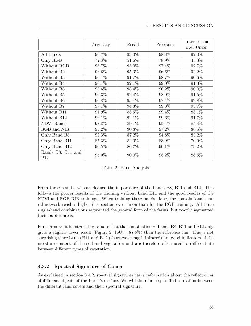
We compared the results of the trainings (Table 2) with different combination of bandsfrom the Ecuadorian Sentinel 2 image. The first run with all the bands (B2, B3, B4, B5,B6, B7, B8, B11 and B12) has an intersection over union of 92.0%. This will be the refer-ence point to compare the other runs.
In a first step, we analyzed the importance of multispectral images by only testing the RGBbands. We observe that the RGB-bands alone (Figure 2: IoU = 45.3%) are not enough toproperly detect cocoa. The cocoa predictions were randomly distributed over the validationarea and did not have the characteristic form of the validation (Figure 16). This means thatthe use of multispectral images and bands further than the visible electromagnetic wavesare important for cocoa segmentation. This statement is further confirmed by the result ofthe training run without the visible bands (Figure 2: IoU = 92.7%); the intersection overunion being comparable to the reference run. This can be explained by the fact that RGBis mostly used for the detection of textural features and structural patterns. This is quiteunnecessary because the image resolution of the Sentinel-2 data is 10 × 10 m and no tex-ture should be recognizable in the images since there is more than one tree per image pixel.
Band B11 (1610 nm) is important, since the run without band B11 only reached an in-tersection over union of 83.1%, nearly 10% less than the reference run. The other bandsdo not show significant differences compared to the reference run when dropping them outduring training.
It is interesting to observe that the traditional methods such as NDVI (B4 and B8) andRGB-NIR (B2, B3, B4 and B8) show comparable results to the reference run with all thebands. The differences in the results between these two methods and the reference run isdue to the accuracy of the predictions in the border region of the farm.
37
4. RESULTS AND DISCUSSION
Accuracy Recall PrecisionIntersectionover Union
All Bands 96.7% 93.0% 98.8% 92.0%
Only RGB 72.3% 51.6% 78.9% 45.3%
Without RGB 96.7% 95.0% 97.4% 92.7%
Without B2 96.6% 95.3% 96.6% 92.2%
Without B3 96.1% 91.7% 98.7% 90.6%
Without B4 96.1% 92.1% 99.0% 91.3%
Without B8 95.6% 93.4% 96.2% 90.0%
Without B5 96.3% 92.4% 98.9% 91.5%
Without B6 96.8% 95.1% 97.4% 92.8%
Without B7 97.1% 94.3% 99.3% 93.7%
Without B11 91.9% 83.5% 99.4% 83.1%
Without B12 96.1% 92.1% 99.6% 91.7%
NDVI Bands 93.8% 89.1% 95.4% 85.4%
RGB and NIR 95.2% 90.8% 97.2% 88.5%
Only Band B8 92.3% 87.2% 94.8% 83.2%
Only Band B11 87.3% 82.0% 83.9% 70.9%
Only Band B12 90.5% 86.7% 90.1% 79.2%
Bands B8, B11 andB12
95.0% 90.0% 98.2% 88.5%
Table 2: Band Analysis
From these results, we can deduce the importance of the bands B8, B11 and B12. Thisfollows the poorer results of the training without band B11 and the good results of theNDVI and RGB-NIR trainings. When training these bands alone, the convolutional neu-ral network reaches higher intersection over union than for the RGB training. All threesingle-band combinations segmented the general form of the farms, but poorly segmentedtheir border areas.
Furthermore, it is interesting to note that the combination of bands B8, B11 and B12 onlygives a slightly lower result (Figure 2: IoU = 88.5%) than the reference run. This is notsurprising since bands B11 and B12 (short-wavelength infrared) are good indicators of themoisture content of the soil and vegetation and are therefore often used to differentiatebetween different types of vegetation.
4.3.2 Spectral Signature of Cocoa
As explained in section 3.4.2, spectral signatures carry information about the reflectancesof different objects of the Earth’s surface. We will therefore try to find a relation betweenthe different land covers and their spectral signature.
38
4. RESULTS AND DISCUSSION
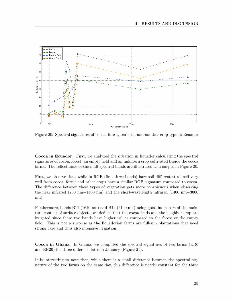
Figure 20: Spectral signatures of cocoa, forest, bare soil and another crop type in Ecuador
Cocoa in Ecuador First, we analyzed the situation in Ecuador calculating the spectralsignatures of cocoa, forest, an empty field and an unknown crop cultivated beside the cocoafarms. The reflectances of the multispectral bands are illustrated as triangles in Figure 20.
First, we observe that, while in RGB (first three bands) bare soil differentiates itself verywell from cocoa, forest and other crops have a similar RGB signature compared to cocoa.The difference between these types of vegetation gets more conspicuous when observingthe near infrared (700 nm−1400 nm) and the short-wavelength infrared (1400 nm−3000nm).
Furthermore, bands B11 (1610 nm) and B12 (2190 nm) being good indicators of the mois-ture content of surface objects, we deduce that the cocoa fields and the neighbor crop areirrigated since these two bands have higher values compared to the forest or the emptyfield. This is not a surprise as the Ecuadorian farms are full-sun plantations that needstrong care and thus also intensive irrigation.
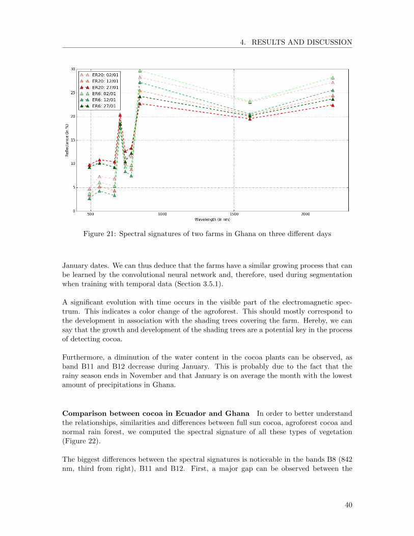
Cocoa in Ghana In Ghana, we computed the spectral signatures of two farms (ER6and ER20) for three different dates in January (Figure 21).
It is interesting to note that, while there is a small difference between the spectral sig-nature of the two farms on the same day, this difference is nearly constant for the three
39
4. RESULTS AND DISCUSSION
Figure 21: Spectral signatures of two farms in Ghana on three different days
January dates. We can thus deduce that the farms have a similar growing process that canbe learned by the convolutional neural network and, therefore, used during segmentationwhen training with temporal data (Section 3.5.1).
A significant evolution with time occurs in the visible part of the electromagnetic spec-trum. This indicates a color change of the agroforest. This should mostly correspond tothe development in association with the shading trees covering the farm. Hereby, we cansay that the growth and development of the shading trees are a potential key in the processof detecting cocoa.
Furthermore, a diminution of the water content in the cocoa plants can be observed, asband B11 and B12 decrease during January. This is probably due to the fact that therainy season ends in November and that January is on average the month with the lowestamount of precipitations in Ghana.
Comparison between cocoa in Ecuador and Ghana In order to better understandthe relationships, similarities and differences between full sun cocoa, agroforest cocoa andnormal rain forest, we computed the spectral signature of all these types of vegetation(Figure 22).
The biggest differences between the spectral signatures is noticeable in the bands B8 (842nm, third from right), B11 and B12. First, a major gap can be observed between the
40
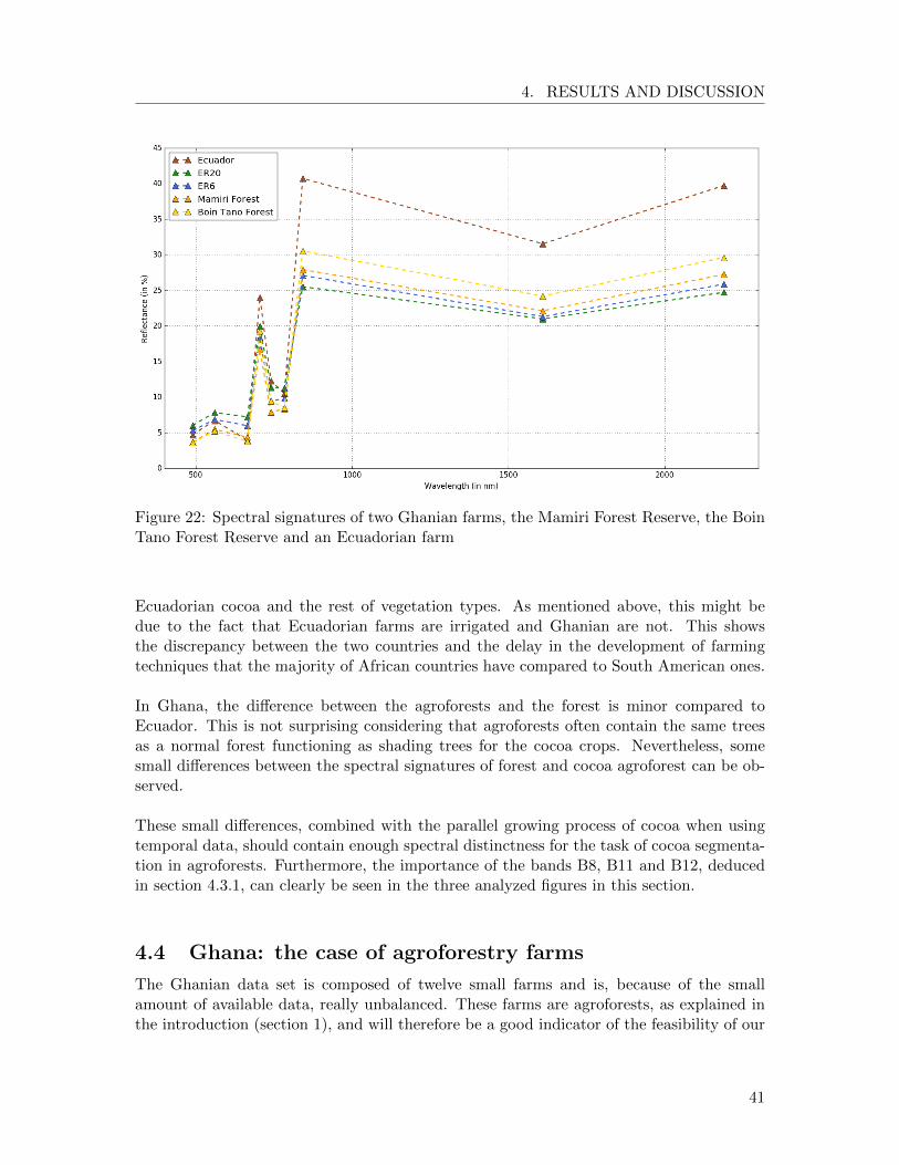
4. RESULTS AND DISCUSSION
Figure 22: Spectral signatures of two Ghanian farms, the Mamiri Forest Reserve, the BoinTano Forest Reserve and an Ecuadorian farm
Ecuadorian cocoa and the rest of vegetation types. As mentioned above, this might bedue to the fact that Ecuadorian farms are irrigated and Ghanian are not. This showsthe discrepancy between the two countries and the delay in the development of farmingtechniques that the majority of African countries have compared to South American ones.
In Ghana, the difference between the agroforests and the forest is minor compared toEcuador. This is not surprising considering that agroforests often contain the same treesas a normal forest functioning as shading trees for the cocoa crops. Nevertheless, somesmall differences between the spectral signatures of forest and cocoa agroforest can be ob-served.
These small differences, combined with the parallel growing process of cocoa when usingtemporal data, should contain enough spectral distinctness for the task of cocoa segmenta-tion in agroforests. Furthermore, the importance of the bands B8, B11 and B12, deducedin section 4.3.1, can clearly be seen in the three analyzed figures in this section.
4.4 Ghana: the case of agroforestry farms
The Ghanian data set is composed of twelve small farms and is, because of the smallamount of available data, really unbalanced. These farms are agroforests, as explained inthe introduction (section 1), and will therefore be a good indicator of the feasibility of our
41
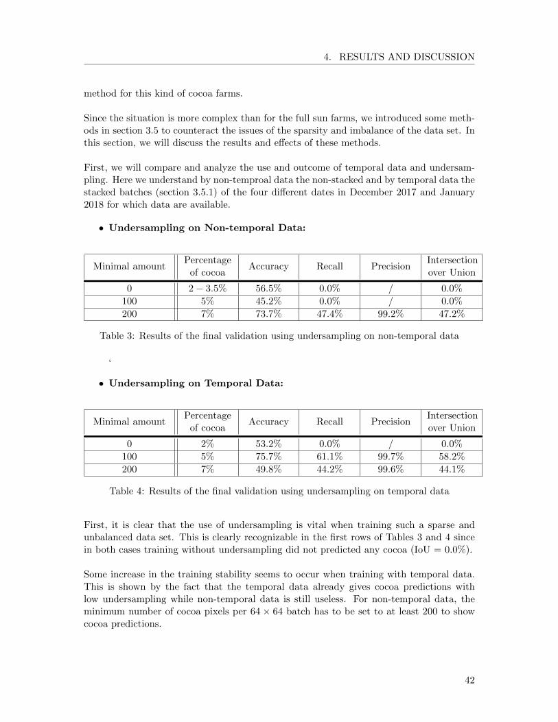
4. RESULTS AND DISCUSSION
method for this kind of cocoa farms.
Since the situation is more complex than for the full sun farms, we introduced some meth-ods in section 3.5 to counteract the issues of the sparsity and imbalance of the data set. Inthis section, we will discuss the results and effects of these methods.
First, we will compare and analyze the use and outcome of temporal data and undersam-pling. Here we understand by non-temproal data the non-stacked and by temporal data thestacked batches (section 3.5.1) of the four different dates in December 2017 and January2018 for which data are available.
• Undersampling on Non-temporal Data:
Minimal amountPercentage
of cocoaAccuracy Recall Precision
Intersectionover Union
0 2 − 3.5% 56.5% 0.0% / 0.0%
100 5% 45.2% 0.0% / 0.0%
200 7% 73.7% 47.4% 99.2% 47.2%
Table 3: Results of the final validation using undersampling on non-temporal data
‘
• Undersampling on Temporal Data:
Minimal amountPercentage
of cocoaAccuracy Recall Precision
Intersectionover Union
0 2% 53.2% 0.0% / 0.0%
100 5% 75.7% 61.1% 99.7% 58.2%
200 7% 49.8% 44.2% 99.6% 44.1%
Table 4: Results of the final validation using undersampling on temporal data
First, it is clear that the use of undersampling is vital when training such a sparse andunbalanced data set. This is clearly recognizable in the first rows of Tables 3 and 4 sincein both cases training without undersampling did not predicted any cocoa (IoU = 0.0%).
Some increase in the training stability seems to occur when training with temporal data.This is shown by the fact that the temporal data already gives cocoa predictions withlow undersampling while non-temporal data is still useless. For non-temporal data, theminimum number of cocoa pixels per 64 × 64 batch has to be set to at least 200 to showcocoa predictions.
42
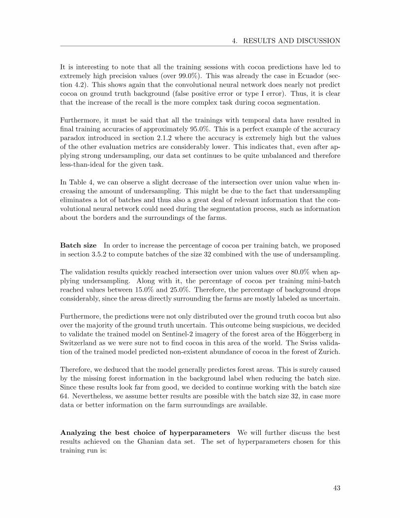
4. RESULTS AND DISCUSSION
It is interesting to note that all the training sessions with cocoa predictions have led toextremely high precision values (over 99.0%). This was already the case in Ecuador (sec-tion 4.2). This shows again that the convolutional neural network does nearly not predictcocoa on ground truth background (false positive error or type I error). Thus, it is clearthat the increase of the recall is the more complex task during cocoa segmentation.
Furthermore, it must be said that all the trainings with temporal data have resulted infinal training accuracies of approximately 95.0%. This is a perfect example of the accuracyparadox introduced in section 2.1.2 where the accuracy is extremely high but the valuesof the other evaluation metrics are considerably lower. This indicates that, even after ap-plying strong undersampling, our data set continues to be quite unbalanced and thereforeless-than-ideal for the given task.
In Table 4, we can observe a slight decrease of the intersection over union value when in-creasing the amount of undersampling. This might be due to the fact that undersamplingeliminates a lot of batches and thus also a great deal of relevant information that the con-volutional neural network could need during the segmentation process, such as informationabout the borders and the surroundings of the farms.
Batch size In order to increase the percentage of cocoa per training batch, we proposedin section 3.5.2 to compute batches of the size 32 combined with the use of undersampling.
The validation results quickly reached intersection over union values over 80.0% when ap-plying undersampling. Along with it, the percentage of cocoa per training mini-batchreached values between 15.0% and 25.0%. Therefore, the percentage of background dropsconsiderably, since the areas directly surrounding the farms are mostly labeled as uncertain.
Furthermore, the predictions were not only distributed over the ground truth cocoa but alsoover the majority of the ground truth uncertain. This outcome being suspicious, we decidedto validate the trained model on Sentinel-2 imagery of the forest area of the Hoggerberg inSwitzerland as we were sure not to find cocoa in this area of the world. The Swiss valida-tion of the trained model predicted non-existent abundance of cocoa in the forest of Zurich.
Therefore, we deduced that the model generally predictes forest areas. This is surely causedby the missing forest information in the background label when reducing the batch size.Since these results look far from good, we decided to continue working with the batch size64. Nevertheless, we assume better results are possible with the batch size 32, in case moredata or better information on the farm surroundings are available.
Analyzing the best choice of hyperparameters We will further discuss the bestresults achieved on the Ghanian data set. The set of hyperparameters chosen for thistraining run is:
43
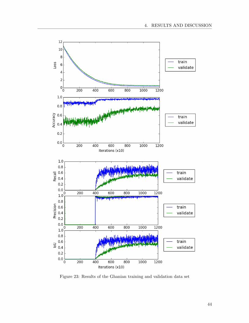
4. RESULTS AND DISCUSSION
Figure 23: Results of the Ghanian training and validation data set
44
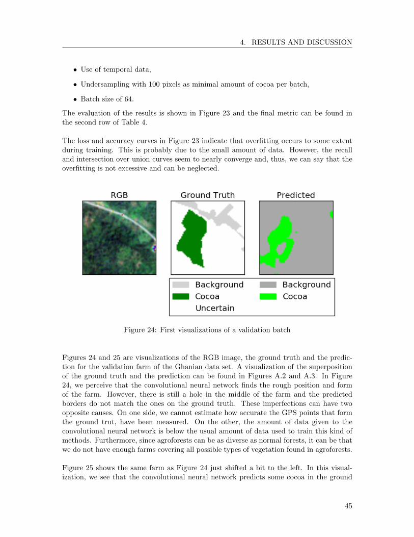
4. RESULTS AND DISCUSSION
• Use of temporal data,
• Undersampling with 100 pixels as minimal amount of cocoa per batch,
• Batch size of 64.
The evaluation of the results is shown in Figure 23 and the final metric can be found inthe second row of Table 4.
The loss and accuracy curves in Figure 23 indicate that overfitting occurs to some extentduring training. This is probably due to the small amount of data. However, the recalland intersection over union curves seem to nearly converge and, thus, we can say that theoverfitting is not excessive and can be neglected.
Figure 24: First visualizations of a validation batch
Figures 24 and 25 are visualizations of the RGB image, the ground truth and the predic-tion for the validation farm of the Ghanian data set. A visualization of the superpositionof the ground truth and the prediction can be found in Figures A.2 and A.3. In Figure24, we perceive that the convolutional neural network finds the rough position and formof the farm. However, there is still a hole in the middle of the farm and the predictedborders do not match the ones on the ground truth. These imperfections can have twoopposite causes. On one side, we cannot estimate how accurate the GPS points that formthe ground trut, have been measured. On the other, the amount of data given to theconvolutional neural network is below the usual amount of data used to train this kind ofmethods. Furthermore, since agroforests can be as diverse as normal forests, it can be thatwe do not have enough farms covering all possible types of vegetation found in agroforests.
Figure 25 shows the same farm as Figure 24 just shifted a bit to the left. In this visual-ization, we see that the convolutional neural network predicts some cocoa in the ground
45
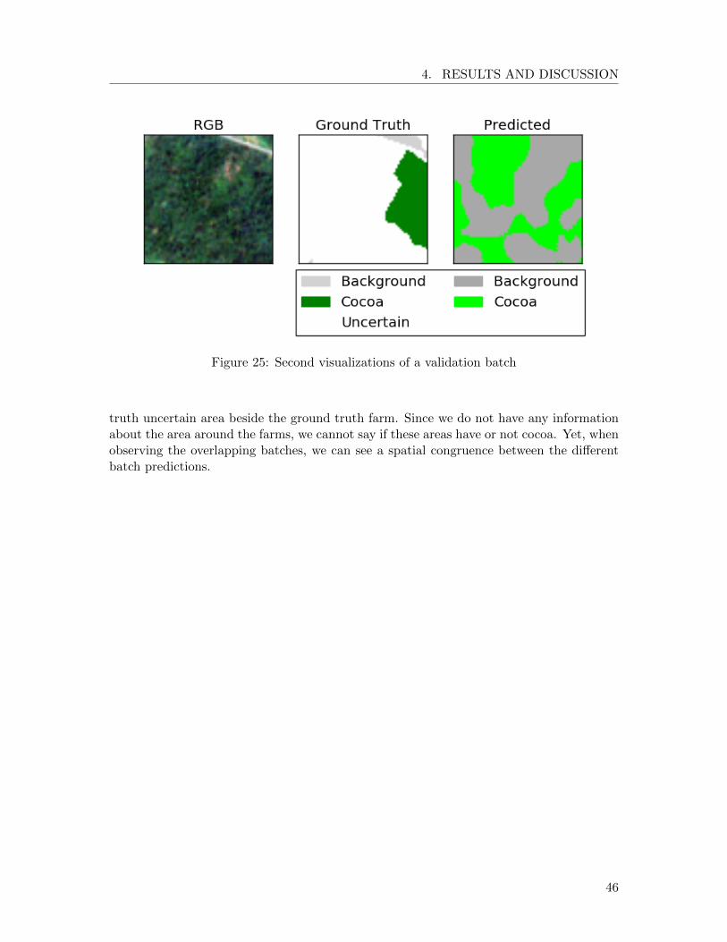
4. RESULTS AND DISCUSSION
Figure 25: Second visualizations of a validation batch
truth uncertain area beside the ground truth farm. Since we do not have any informationabout the area around the farms, we cannot say if these areas have or not cocoa. Yet, whenobserving the overlapping batches, we can see a spatial congruence between the differentbatch predictions.
46
5. CONCLUSIONS
5 Conclusions
The main aim of this Bachelor’s thesis was to test the feasibility of cocoa segmentationby combining the use of satellite multispectral imagery and deep learning methods. Thesecond objective was to analyze and, thus, understand the learning process and determinethe decisive properties of convolutional neural networks and multispectral images duringcocoa segmentation. Considering that cocoa is cultivated with different methods depend-ing on the country, we analyzed our method separately for full sun farms and agroforestyfarms, using Ecuador and Ghana as representatives for both farming methods.
We can assert that the method developed during this project works very well for full sunfarms, such as the ones found in countries like Ecuador. However, since these remarkableresults have only been achieved on two farms, they need to be validated using a biggerdata set with larger amounts of farms distributed trough Ecuador or, even, with farmsfrom other countries using full sun farming.
We showed the need for multispectral imagery and information of near-infrared and short-wavelength infrared reflectance for the task of cocoa segmentation. Along with it, we founda significant difference between the spectral signature of cocoa cultivated in full sun farmsand agroforests. This reinforces the initial decision to treat full sun cocoa and agroforestcocoa farms separately.
In the case of agroforestry, we cannot affirm the applicability of our method due to the un-certainty associated with of our results. However, they indicate some promising directionstowards the use of this method for agroforestry.
Furthermore, we propose some improvements and next steps for our project:
• Implementing a more powerful architecture.
• Increasing the amount of data not only in Ghana but also in Ecuador. This willsolve the issue of the data sparsity and additionally decrease the imbalance of thedata set. In addition, it will further validate our results and give the possibility ofdefinitively proving the feasibility of the method.
• Increasing the information of the surrounding of the farms. This will, on the onehand, counteract the imbalance of the data set and, on the other hand, validate thecocoa predictions that at this point of the project are still uncertain.
• Implementing a method to detect clouds and threat them separately from the restof the data set. This should be integrated in a complete and more sophisticated man-agement of the cloud problem that occurs when using satellite multispecral imageryin tropical regions.
• As a consequence of the previous point, introducing more labels to separate differenttype of crops and vegetation. This will increase the complexity of the model andhelp the convolutional neural network to better understand the surrounding of the
47
5. CONCLUSIONS
agroforest farms. For instance, improving its ability to separate streets from differenttypes of vegetation. Of course, this requires that the surrounding of the farms isaccurately mapped.
• Computing larger time series. In a future step, the idea of temporal data could begeneralized to all available cloud free Sentinel-2 images over a span of a year. Thiswill increase the amount of information, not only of the cocoa growth, but also ofother types of vegetation such as shading trees that form part of an agroforest.
• Adding batches of uncultivated forest to the data set. This will, when usingundersampling, help to give the convolutional neural network enough informationabout other types of vegetation to distinguish between normal forest and agroforest.
• Implementing a penalization method for errors on the minority class of the un-balanced data set. This will force the convolutional neural network to take this classmore into account.
• As a last step, performing a hyperparameter fine-tuning will allow us to findthe optimal set of hyperparameters for cocoa segmentation and, thus, also the bestpossible results.
48
References
Bibliography
Asare, R. et al. (Dec. 2014). “Cocoa agroforestry for increasing forest connectivity in afragmented landscape in Ghana”. In: Agroforestry Systems 88, pp. 1143–1156.
Barima, Y. et al. (2016). “Cocoa crops are destroying the forest reserves of the classifiedforest of Haut-Sassandra (Ivory Coast)”. English. In: Global Ecology and Conservation8.Complete, pp. 85–98.
Duchi, J., E. Hazan, and Y. Singer (July 2011). “Adaptive Subgradient Methods for OnlineLearning and Stochastic Optimization”. In: J. Mach. Learn. Res. 12, pp. 2121–2159. issn:1532-4435.
Duveiller, G. et al. (2008). “Deforestation in Central Africa: Estimates at regional, nationaland landscape levels by advanced processing of systematically-distributed Landsat ex-tracts”. In: Remote Sensing of Environment 112.5. Earth Observations for TerrestrialBiodiversity and Ecosystems Special Issue, pp. 1969–1981. issn: 0034-4257.
Ellis, E. and N. Ramankutty (2008). “Putting people in the map: anthropogenic biomes ofthe world”. In: Frontiers in Ecology and the Environment 6.8, pp. 439–447.
He, K. et al. (2015). “Deep Residual Learning for Image Recognition”. In: CoRR abs/1512.03385.
Heusel, M. et al. (2017). “GANs Trained by a Two Time-Scale Update Rule Converge toa Nash Equilibrium”. In: CoRR abs/1706.08500.
Inglada, J. et al. (2016). “Improved Early Crop Type Identification By Joint Use of HighTemporal Resolution SAR And Optical Image Time Series”. In: Remote Sensing.
Ioffe, S. and C. Szegedy (2015). “Batch Normalization: Accelerating Deep Network Trainingby Reducing Internal Covariate Shift”. In: CoRR abs/1502.03167.
Ivakhnenko, A. G. (1965). Cybernetic Predicting Devices. CCM Information Corporation.
Karpathy, A. (2018). CS231n: Convolutional Neural Networks for Visual Recognition. Stan-ford CS. url: http://cs231n.github.io/.
Kent, A. et al. (1955). “Machine literature searching VIII. Operational criteria for designinginformation retrieval systems”. In: American Documentation 6.2, pp. 93–101.
Kingma, D. and J. Ba (2014). “Adam: A Method for Stochastic Optimization”. In: CoRRabs/1412.6980.
49
Krizhevsky, A., I. Sutskever, and G. Hinton (2012). “ImageNet Classification with DeepConvolutional Neural Networks”. In: Advances in Neural Information Processing Systems25. Ed. by F. Pereira et al. Curran Associates, Inc., pp. 1097–1105.
LeCun, Y. et al. (Sept. 1989). “Backpropagation Applied to Handwritten Zip Code Recog-nition”. In: Neural Computation 1.4, pp. 541–551. issn: 0899-7667.
– (Dec. 1998). “Gradient-Based Learning Applied to Document Recognition”. In: Proceed-ings of the IEEE 86, pp. 2278–2324.
Nowaczynski, A. et al. (2017). Deep learning for satellite imagery via image segmentation.Blog post.
Obiri, B. et al. (Oct. 2007). “Financial analysis of shaded cocoa in Ghana”. In: AgroforestrySystems 71, pp. 139–149.
Ronneberger, O., P. Fischer, and T. Brox (2015). “U-Net: Convolutional Networks forBiomedical Image Segmentation”. In: CoRR abs/1505.04597.
Ruf, F. (2007). “Current Cocoa production and opportunities for re-investment in the ruralsector. Cote d’Ivoire, Ghana and Indonesia.” In: World Cocoa Foundation, Amsterdam,23-24 May 2007.
– (2011). “The Myth of Complex Cocoa Agroforests: The Case of Ghana”. In: HumanEcology 39.3, pp. 373–388.
Snapir, B., D.M. Simms, and T.W. Waine (2017). “Mapping the expansion of galamsey goldmines in the cocoa growing area of Ghana using optical remote sensing”. In: InternationalJournal of Applied Earth Observation and Geoinformation 58, pp. 225–233. issn: 0303-2434.
Srivastava, N. et al. (2014). “Dropout: A Simple Way to Prevent Neural Networks fromOverfitting”. In: Journal of Machine Learning Research 15, pp. 1929–1958.
Wegner, J. D. (2017). 103-0274-00L Bildverarbeitung. Lecture, ETH Zurich. Course at ETHZurich.
50
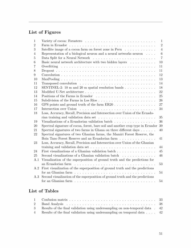
List of Figures
1 Variety of cocoa: Forastero . . . . . . . . . . . . . . . . . . . . . . . . . . . 12 Farm in Ecuador . . . . . . . . . . . . . . . . . . . . . . . . . . . . . . . . . 23 Satellite image of a cocoa farm on forest zone in Peru . . . . . . . . . . . . 44 Representation of a biological neuron and a neural networks neuron . . . . 65 Data Split for a Neural Network . . . . . . . . . . . . . . . . . . . . . . . . 76 Basic neural network architecture with two hidden layers . . . . . . . . . . 107 Overfitting . . . . . . . . . . . . . . . . . . . . . . . . . . . . . . . . . . . . 118 Dropout . . . . . . . . . . . . . . . . . . . . . . . . . . . . . . . . . . . . . . 119 Convolution . . . . . . . . . . . . . . . . . . . . . . . . . . . . . . . . . . . . 1210 MaxPooling . . . . . . . . . . . . . . . . . . . . . . . . . . . . . . . . . . . . 1311 Transposed convolution . . . . . . . . . . . . . . . . . . . . . . . . . . . . . 1412 SENTINEL-2: 10 m and 20 m spatial resolution bands . . . . . . . . . . . . 1813 Modified U-Net architecture . . . . . . . . . . . . . . . . . . . . . . . . . . . 2214 Positions of the Farms in Ecuador . . . . . . . . . . . . . . . . . . . . . . . 2515 Subdivision of the Farms in Los Rıos . . . . . . . . . . . . . . . . . . . . . . 2616 GPS points and ground truth of the farm ER20 . . . . . . . . . . . . . . . . 2717 Intersection over Union . . . . . . . . . . . . . . . . . . . . . . . . . . . . . 3418 Loss, Accuracy, Recall, Precision and Intersection over Union of the Ecuado-
rian training and validation data set . . . . . . . . . . . . . . . . . . . . . . 3519 Visualizations of a Ecuadorian validation batch . . . . . . . . . . . . . . . . 3620 Spectral signature of cocoa, forest, bare soil and another crop type in Ecuador 3921 Spectral signatures of two farms in Ghana on three different days . . . . . . 4022 Spectral signatures of two Ghanian farms, the Mamiri Forest Reserve, the
Boin Tano Forest Reserve and an Ecuadorian farm . . . . . . . . . . . . . . 4123 Loss, Accuracy, Recall, Precision and Intersection over Union of the Ghanian
training and validation data set . . . . . . . . . . . . . . . . . . . . . . . . . 4424 First visualizations of a Ghanian validation batch . . . . . . . . . . . . . . . 4525 Second visualizations of a Ghanian validation batch . . . . . . . . . . . . . 46A.1 Visualization of the superposition of ground truth and the predictions for
an Ecuadorian farm . . . . . . . . . . . . . . . . . . . . . . . . . . . . . . . 53A.2 First visualization of the superposition of ground truth and the predictions
for an Ghanian farm . . . . . . . . . . . . . . . . . . . . . . . . . . . . . . . 54A.3 Second visualization of the superposition of ground truth and the predictions
for an Ghanian farm . . . . . . . . . . . . . . . . . . . . . . . . . . . . . . . 54
List of Tables
1 Confusion matrix . . . . . . . . . . . . . . . . . . . . . . . . . . . . . . . . . 332 Band Analysis . . . . . . . . . . . . . . . . . . . . . . . . . . . . . . . . . . 383 Results of the final validation using undersampling on non-temporal data . 424 Results of the final validation using undersampling on temporal data . . . . 42
51

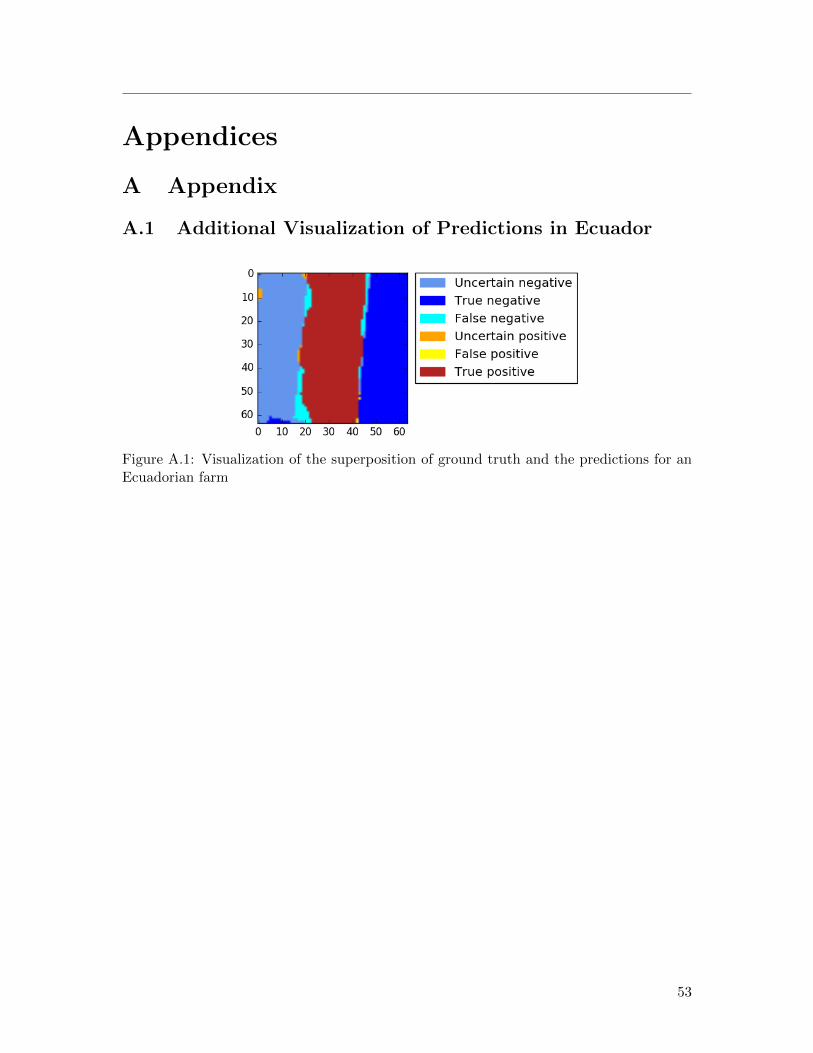
Appendices
A Appendix
A.1 Additional Visualization of Predictions in Ecuador
Figure A.1: Visualization of the superposition of ground truth and the predictions for anEcuadorian farm
53
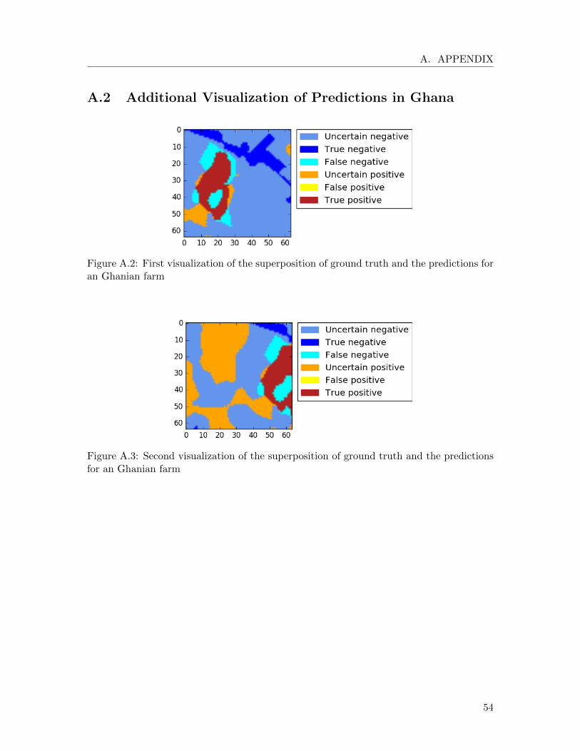
A. APPENDIX
A.2 Additional Visualization of Predictions in Ghana
Figure A.2: First visualization of the superposition of ground truth and the predictions foran Ghanian farm
Figure A.3: Second visualization of the superposition of ground truth and the predictionsfor an Ghanian farm
54