Coastal Typology Development with Heterogeneous DataSets

Bruce A. Maxwell Robert W. BuddemeierSwarthmore College Kansas Geological Survey

Swarthmore, PA 19081 Lawrence, KS 66047maxwell@swarthmore.edu buddrw@kgs.ukans.edu

(610)328-8081 (phone)(610)328-8082 (fax)

Coastal Typology Development with Heterogeneous DataSets

AbstractThis paper presents a data-driven expert-guided method of coastal typology development using alarge, heterogeneous data set. The development of coastal typologies is driven by a desire toupscale detailed regional information to a global scale in order to study coastal zone function andthe effects of global climate change. We demonstrate two methods of automatic typology genera-tion--unsupervised clustering and region growing with agglomerative clustering--and a method ofselecting an appropriate number of classes based on the concept of Minimum Description Length.We compare two methods of defining distance between data points with a large number of vari-ables and potentially missing data--average scaled Euclidean distance and maximum scaled dif-ference. To visualize the resulting typologies we use a novel algorithm for assigning colors todifferent classes of data based on class similarity in a high-dimensional space. This combinationof techniques results in a methodology through which one or more experts can easily develop auseful coastline typology with results that are similar to pre-existing expert typologies, but whichmakes the process more quantitative, objective, consistent, and applicable across space and time.

Keywords: coastal zone, typology, clustering, visualization, distance measure

1 Introduction

The Land-Ocean Interaction in the Coastal Zone project [LOICZ] is a component of the Interna-tional Geosphere-Biosphere Programme [IGBP] that focuses on the area of the earth’s surfacewhere land, ocean and atmosphere meet and interact. The overall goal of this project is to deter-mine at regional and global scales: the nature of that dynamic interaction; how changes in variouscompartments of the Earth system are affecting coastal zones and altering their role in globalcycles; to assess how future changes in these areas will affect their use by people; and, to providea sound scientific basis for future integrated management of coastal areas on a sustainable basis[14].

A primary LOICZ objective is developing global scale-estimates of biogeochemical fluxes of car-bon, nitrogen, and phosphorous [C, N and P] in and through the coastal zone [CZ] [5]. The strat-egy adopted is to identify ‘type-specimen’ CNP budgets for well-characterized coastal regions, tofurther identify the coastal regions around the world of which such functional observations mightbe typical, and to use this typology relationship to upscale the limited local data to an estimate ofglobal coastal zone function. Within this context, a typology is defined as a classification systemthat divides coastal zones into a set of classes according to one or more physical, geological,atmospheric, or human-related variables.

The development of an inventory of standard-format CZ budgets is in progress in the Bio-geochemical Budgets task of LOICZ (http://data.ecology.su.se/mnode/). The Typology project(http://www.nioz.nl/loicz/typo.htm) is responsible for developing the coastal classificationapproach needed for budget upscaling. One of the major strategies adopted is the development ofclustering and visualization techniques suitable for classifying coastal areas in terms of their sim-ilarity with respect to environmental variables relevant to biogeochemical function.

The task is challenging because of the need to rely on globally-available data, and to incorporatemany different types of variables -- marine, terrestrial, climatic, biotic, and “human dimension”(i.e., socioeconomic and environmental alteration). Although a variety of data is available, datasets differ in format, resolution, classes, and completeness, and the data themselves are typicallynot normally distributed or amenable to standard statistical analyses.

Traditional approaches to typology development for geospatial data take either a top-down or bot-tom-up approach. In a top-down approach experts design a decision tree based on different vari-ables and variable ranges that seem appropriate for the environment being considered[10][19][20]. The experts then apply this scheme to a data set and iteratively refine the classifica-tions. A variation on this approach is to have experts classify a training set for a pattern classifier--either symbolic or subsymbolic like an artificial neural network--and then have the pattern classi-fier learn the classes from the training set and generalize the classification strategy to unseen data.

In the bottom-up approach, a clustering method is used to determine groups of similar data pointswhich then form standard classes. Traditional clustering methods include agglomerative cluster-ing and the K-means clustering algorithm, also known as Vector Quantization [VQ][1][7][12][17]. In a geographic/geological context, researchers have used a variation on bottom-up clustering termed regionalization, which locates spatially contiguous class members afterapplying a general agglomerative clustering to the data set that ignores spatial location [6].Researchers have also used K-means clustering on Landsat-4 data to examine the geographic dif-ferences between coastal areas of large lakes [13]. In both of these cases the data sets were fullypopulated and the number of variables small and statistically well-behaved.

In the top-down typology approach, the result is dependent upon expert decisions. In a bottom-upapproach, the resulting typology is affected by two major issues, both of which can be guided byexpert input. First, how many classes should there be in the typology? Second, how do we mea-sure similarity between data points? The second is especially important when we consider multi-dimensional heterogeneous vectors--data points that have multiple variables with different ranges,variances, and meanings.

The answer we propose to the first question--how many classes?--is that expert opinion guided bydata analysis is most appropriate. The data analysis we propose using in section 2.4 is an informa-tion theoretic criterion that balances the costs and benefits of using more or fewer classes. If weused agglomerative clustering--which generates a tree, or dendogram of classification schema forall possible numbers of clusters--then the expert user would generally select the appropriate level.As we note below, our information theoretic criterion would also apply in this situation

The traditional answer to the second question--how do you measure similarity of heterogeneousdata?--is to use a statistical measure that incorporate variances and covariances of the variables.However, when dealing with potentially incomplete heterogeneous global data sets at differentscales, traditional techniques begin to break down. The first casualty is that the covariance matrixbecomes non-invertible, making it impossible to use the Mahalanobis distance that handles cova-riances. The second casualty is that with missing variables in some locations we cannot use a sim-ple “sum-of” technique because different pairs of data points will sum different numbers ofvalues. In sections 2.1 and 2.2 we present our solutions, which include two measures that degradegracefully in the face of missing data and still incorporate variance information.

In section 3 we present the results of typology development on Australasia, which is a good exam-ple location because of the existence of both expert typologies for the region and a large numberof budget sites which we can use for flux estimation [19]. In section 4 we discuss the results andpresent directions for future work. Finally, we conclude with a summary of the typology develop-ment process in section 5.

2 Theory and methodology

Before we can begin to develop classifications and typologies, we must first define what we meanwhen we say two data points are similar. Only then can we think about grouping similar pointsand building conceptual structures. With a mathematical definition of similarity, we can bring tobear numerous useful concepts and algorithms from statistics and pattern recognition. This sec-tion defines two reasonable definitions of similarity and then presents a suite of algorithms thatuse these definitions for typology development.

2.1 Traditional distance measures for heterogeneous dataA useful way to think about similarity is as the distance between two data points. If the two pointsare similar, the distance between them is small. As their similarity decreases, the distance betweenthem gets larger.

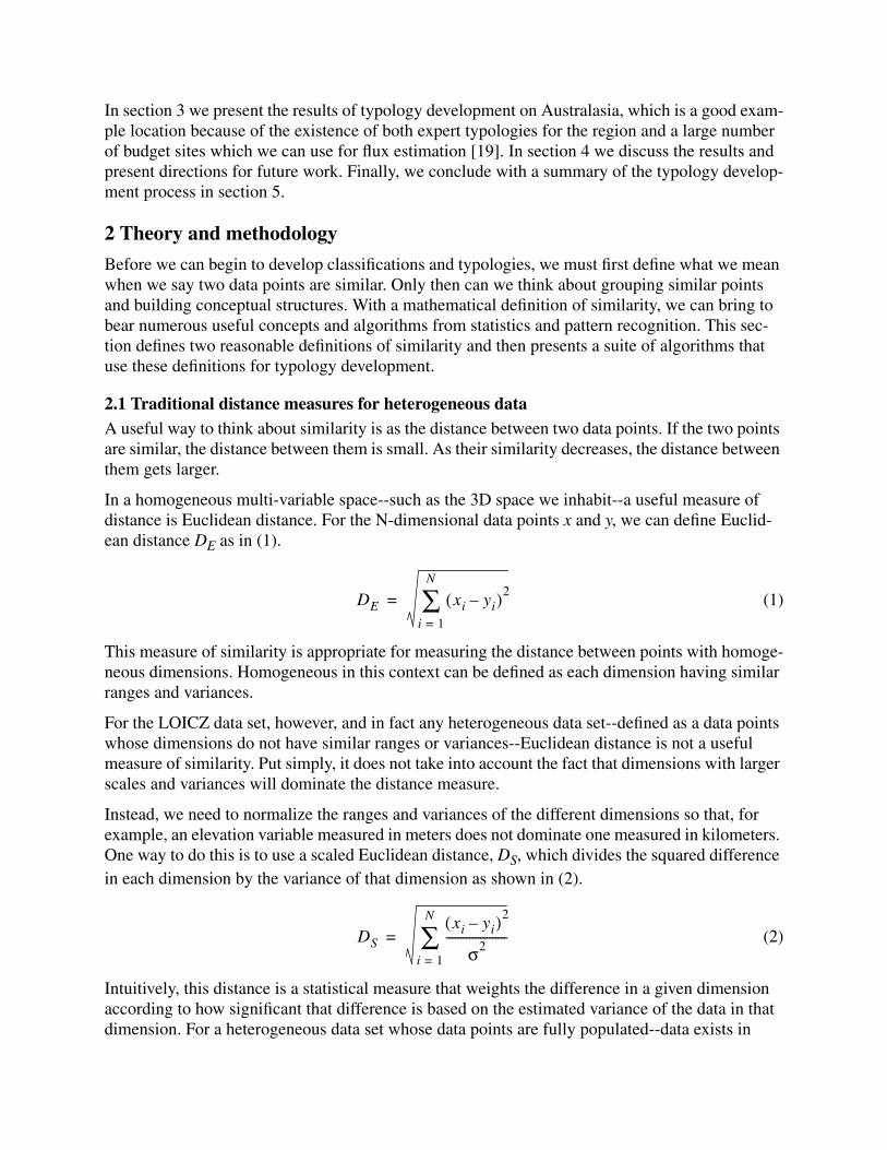
In a homogeneous multi-variable space--such as the 3D space we inhabit--a useful measure ofdistance is Euclidean distance. For the N-dimensional data points x and y, we can define Euclid-ean distance DE as in (1).

(1)

This measure of similarity is appropriate for measuring the distance between points with homoge-neous dimensions. Homogeneous in this context can be defined as each dimension having similarranges and variances.

For the LOICZ data set, however, and in fact any heterogeneous data set--defined as a data pointswhose dimensions do not have similar ranges or variances--Euclidean distance is not a usefulmeasure of similarity. Put simply, it does not take into account the fact that dimensions with largerscales and variances will dominate the distance measure.

Instead, we need to normalize the ranges and variances of the different dimensions so that, forexample, an elevation variable measured in meters does not dominate one measured in kilometers.One way to do this is to use a scaled Euclidean distance, DS, which divides the squared differencein each dimension by the variance of that dimension as shown in (2).

(2)

Intuitively, this distance is a statistical measure that weights the difference in a given dimensionaccording to how significant that difference is based on the estimated variance of the data in thatdimension. For a heterogeneous data set whose data points are fully populated--data exists in

DE xi yi–( )2

i 1=

N

∑=

DS

xi yi–( )2

σ2---------------------

i 1=

N

∑=

every dimension of every point--this definition of distance is reasonable. For a heterogeneous dataset whose data points are not fully populated in every dimension, such as the LOICZ data set, weneed to deal with the missing data.

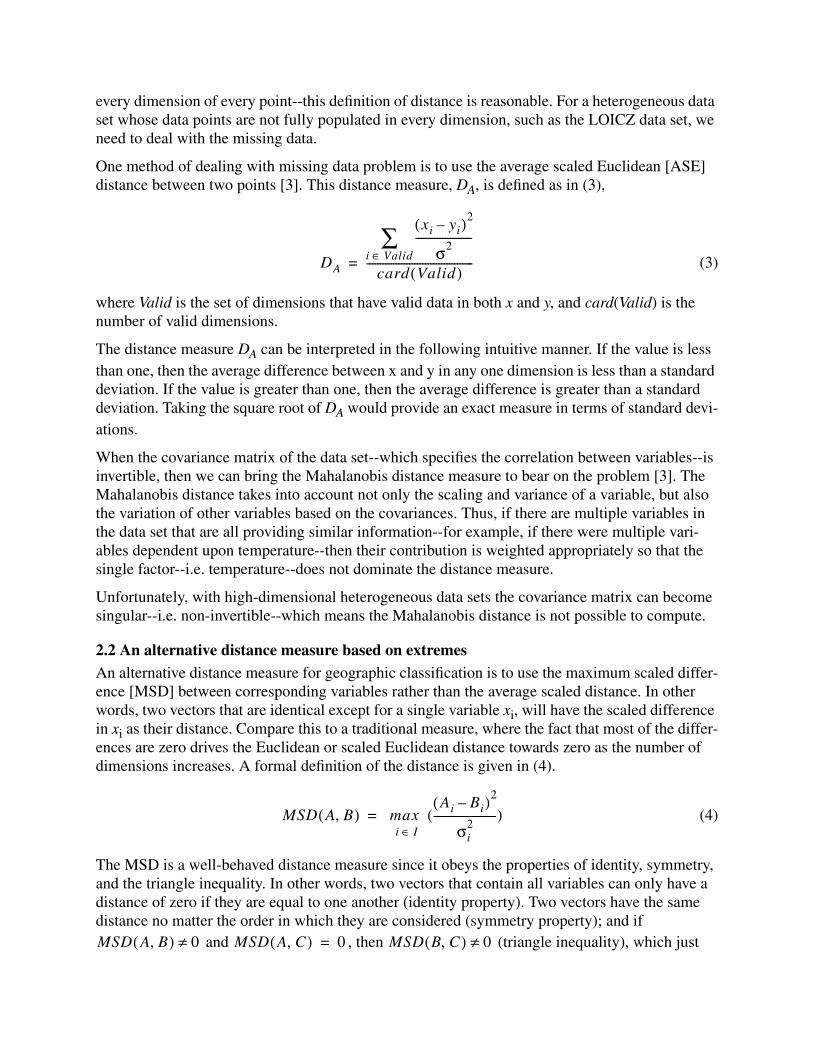
One method of dealing with missing data problem is to use the average scaled Euclidean [ASE]distance between two points [3]. This distance measure, DA, is defined as in (3),

(3)

where Valid is the set of dimensions that have valid data in both x and y, and card(Valid) is thenumber of valid dimensions.

The distance measure DA can be interpreted in the following intuitive manner. If the value is lessthan one, then the average difference between x and y in any one dimension is less than a standarddeviation. If the value is greater than one, then the average difference is greater than a standarddeviation. Taking the square root of DA would provide an exact measure in terms of standard devi-ations.

When the covariance matrix of the data set--which specifies the correlation between variables--isinvertible, then we can bring the Mahalanobis distance measure to bear on the problem [3]. TheMahalanobis distance takes into account not only the scaling and variance of a variable, but alsothe variation of other variables based on the covariances. Thus, if there are multiple variables inthe data set that are all providing similar information--for example, if there were multiple vari-ables dependent upon temperature--then their contribution is weighted appropriately so that thesingle factor--i.e. temperature--does not dominate the distance measure.

Unfortunately, with high-dimensional heterogeneous data sets the covariance matrix can becomesingular--i.e. non-invertible--which means the Mahalanobis distance is not possible to compute.

2.2 An alternative distance measure based on extremesAn alternative distance measure for geographic classification is to use the maximum scaled differ-ence [MSD] between corresponding variables rather than the average scaled distance. In otherwords, two vectors that are identical except for a single variable xi, will have the scaled differencein xi as their distance. Compare this to a traditional measure, where the fact that most of the differ-ences are zero drives the Euclidean or scaled Euclidean distance towards zero as the number ofdimensions increases. A formal definition of the distance is given in (4).

(4)

The MSD is a well-behaved distance measure since it obeys the properties of identity, symmetry,and the triangle inequality. In other words, two vectors that contain all variables can only have adistance of zero if they are equal to one another (identity property). Two vectors have the samedistance no matter the order in which they are considered (symmetry property); and if

and , then (triangle inequality), which just

DA

xi yi–( )2

σ2---------------------

i Valid∈∑card Valid( )

----------------------------------------=

MSD A B,( ) maxi I∈

Ai Bi–( )2

σi2

-----------------------( )=

MSD A B,( ) 0≠ MSD A C,( ) 0= MSD B C,( ) 0≠

states that if two points are not equal, they cannot both be equal to some third point. The MSDalso behaves nicely both with respect to missing variables--it just considers variables that exist inboth data points--and multiple variables that carry the same information--it considers only themaximum difference.

Another way of thinking about the MSD is that it lets the extremes rule judgements of similarity;two vectors cannot be similar if they have a single variable that is very different. In our implemen-tation of MSD distance, we use the maximum normalized squared difference, where the normal-ization constants are the variances of the specific variables.

In some ways, this distance measure may better capture what we think of as similarity in coast-lines. Two habitats that are very much the same except for one variable--such as temperature orprecipitation--may end up being very different. Conversely, we would think of two locations thathave small differences in all variables as being fairly similar. The average scaled Euclidean dis-tance could rate both of these cases as being equally similar, but the MSD distance would say thelatter case--lots of small variations--should be more similar. Thus, the MSD distance starts to cap-ture some of our intuition on the problem.

Other researchers have also attempted to use alternatives to a Euclidean-based distance for envi-ronmental classifications. One example is to use a multi-dimensional scaling approach where therank of a data point’s distance to another data point is weighted more than the actual distance [4].

The MSD distance is inspired by the Hausdorff distance, which is a measure of similarity betweensets that has been used successfully in image comparisons and object recognition tasks in the fieldof computer vision [8]. It has also recently been used in data mining applications to select vari-ables and build decision trees [15]. The Hausdorff distance says that the distance between two setsA and B is the maximum of the minimum distances between all points in A and all points in B.

2.3 Unsupervised k-means clusteringGiven a definition of similarity, we can now start to look for natural groupings of similar pointsthat may indicate the existence of a meaningful class. A standard method for clustering similarpoints is unsupervised k-means clustering, also called vector quantization [VQ][7][12] [17].Overall, the algorithm takes as input a distance measure, a data set, and a desired number of clus-ters. It then attempts to find a set of vectors that best represents the data set. Each of these vectorsis the mean vector of a unique subset of the data points. The output of the VQ algorithm is the setof mean cluster vectors and a tag for each data point, indicating its cluster membership.

The algorithm is briefly defined below. The inputs to the algorithm are the distance measure D(P1,P2), the number of clusters K, and the data points Q[1..N]. The output is a set of mean cluster vec-tors V[1..K].

Assign randomly selected data points to V[1..K]

Loop

Calculate a tag value for each data point Q[1..N]

The tag is the index of the closest V[i] according to D()

Calculate a new set of mean cluster vectors V’[1..K]

If V’ is the same as V then terminate

Else V gets V’ and the loop continues

Return V

Since there is a random element to the VQ algorithm, it is important to run it multiple times withthe same inputs. The best set of cluster vectors V is the set that minimizes the overall representa-tion error, which can be defined as the sum of the distances between each point and its nearestmean cluster vector.

2.4 Using description length to determine the optimal number of clustersOne problem with the VQ algorithm for typology development is that the user must specify thenumber of clusters beforehand. If an expert has some idea of the number of desired clusters, this isnot a problem. However, the expert may not know a priori how many natural clusters there are.

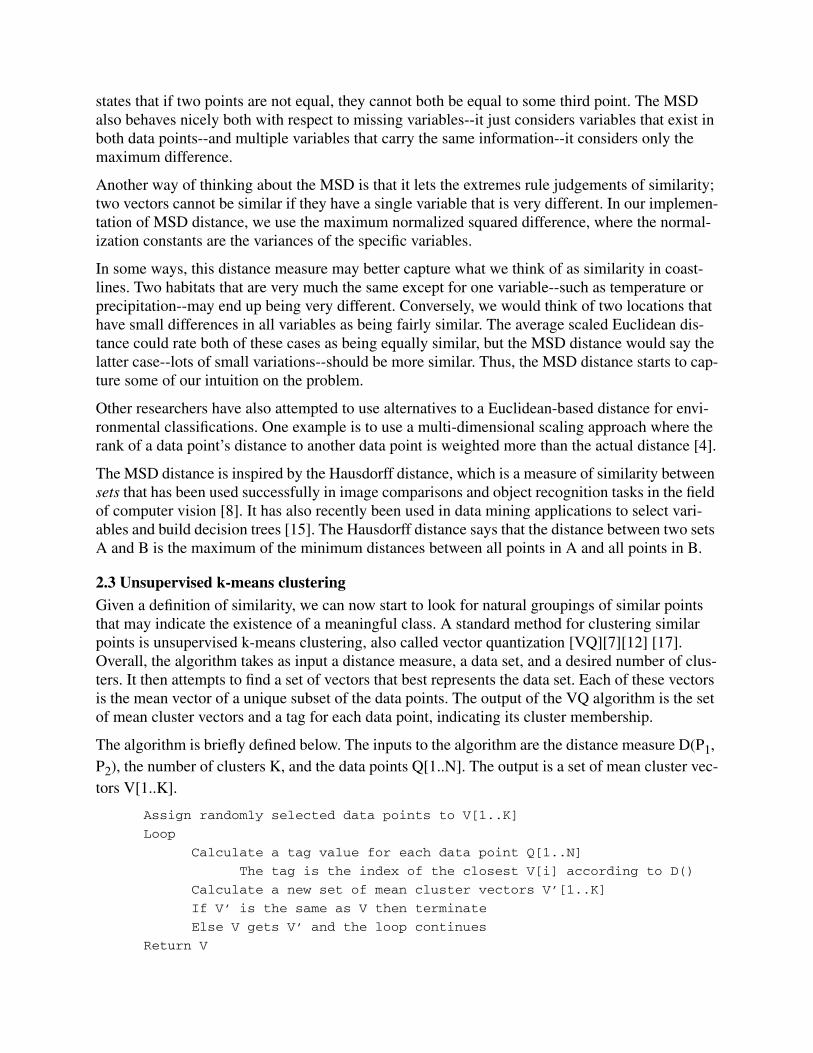
One way to approach this problem is to look for a natural breakpoint in the error as the number ofclusters increases. As the number of clusters gets larger, the representation error tends to zero--which it will become when there are as many clusters as there are data points. Figure 1 shows aplot of error versus the number of clusters that demonstrates this tendency. However, the utility ofincreasing the number of clusters is not a constant function. At some point, the reduction in therepresentation error is not worth adding another cluster.

To generate the error information, we first specify a range of K values and run the VQ algorithmmultiple times for each K. A plot of the resulting error values relative to the number of clustersprovides a graphical description of the benefit of increasing the number of clusters, as shown inFigure 1. In this plot there appear to be two natural breakpoints in this plot, one around 5 clustersand another around 10. This indicates that the first five clusters are critical, the next five are stillsignificantly decreasing the error, and beyond 10 clusters the benefit of using more clusters isminimal. For this example, which is a 3-variable data set constituting the Australian, Oceania, andNew Zealand coastlines, therefore, a 10 class typology would be appropriate.

Note that we can take a more rigorous approach to determining how many clusters is appropriate.The Minimum Description Length Principle, as defined by Rissanen, gives us a mathematical wayof defining when we have enough clusters [18]. Rissanen provides an information-theoretic defi-nition of description length that is a combination of the number of parameters in a model plus therepresentational error for that model. The best model balances these two factors so that their sum

Figure 1. Plot of representation error versus number of clusters for a 3 variable data setfor the Australia Coast

Number of Clusters

Averageerror perdimension

DescriptionLength

is minimized. In the context of clustering, the model is the set of average cluster vectors that rep-resent the data set; and the representational error for a given model is the sum of the squared dis-tances between each point and its associated average cluster vector. The description lengthequation is given in (5).

(5)

This says that the description length DL is equal to the log of the probability of the data (xn) giventhe model (Θ) plus the number of model parameters k multiplied by the log of the number of datapoints. For the LOICZ data set and our definition of distance, the probability of the data given amodel--e.g. the set of mean cluster vectors--is the sum of the squared average scaled distancesfrom each point to its associated mean cluster vector multiplied by the number of variables perpoint. The number of parameters is the number of variables per point multiplied by the number ofclusters. Note that since the number of variables per point is in both terms of the equation weleave it out when calculating the description length.

A plot of the description length for each cluster is given in Figure 1. Note that the minimumdescription length is reached between 9-12 clusters and begins to get larger again beyond that.Therefore, by this measure--a bit more rigorous than the eyeball--we should be using 9-12 clustersto represent this set of coastline data.

2.5 Segmentation through region growingWhereas clustering is, in a sense, a global algorithm, we can also take a local approach to deter-mining groups of similar data points. Since the LOICZ data has a geographic context, it makessense to identify contiguous sections of coastline consisting of similar data points. The clusteringapproach described above does not necessarily take into account geographic considerations whendeciding what data points are alike, although this has been done by other researchers [16].

Region growing is a commonly used technique in computer vision, where local context isextremely important. The basic idea is to begin with a seed point and then add neighboring pointsto that region as long as they are A) similar enough to their neighbor and B) similar enough to theseed region. Note that the requirement for neighboring points to be similar--which we can defineas a local threshold--is usually tighter than the requirement for points to be similar to the seedregion--which we can define as a global threshold. When one region stops growing--because itsneighbors are too different--then we can select a second seed point and grow another region. Thisprocess continues until all data points are labeled.

The result of this process is a set of connected regions consisting of similar pixels. How manyregions there are is dependent upon the local and global thresholds that control the growing pro-cess. If the thresholds are rigorous there will be more regions; if the thresholds are loose there willbe fewer. Note that this approach removes the need to specify the number of clusters, but replacesit with the specification of the local and global similarity thresholds.

What a region growing algorithm provides is a starting point for building a hierarchy based onvariable sized contiguous building blocks.

DL P xn Θ( )log–

k2--- nlog+=

2.6 Methods for merging regionsOnce we have a set of regions--whether found through clustering or region growing--we maywant to merge similar regions together regardless of their spatial location. Especially in the caseof region growing, where all regions are spatially contiguous, it is important to begin matching updiscontinuous but similar stretches of coastline.

We can use a step-wise optimal approach to merging--also called agglomerative clustering [1]--which iteratively merges the two regions with the closest mean cluster vectors. Membership in acluster is strictly maintained with the hierarchy that develops. The algorithm for selecting andmerging two regions is as follows:

Find the pair of mean cluster vectors with minimum distance

Give all the data points in both clusters the same label

Calculate a mean cluster vector for the new cluster

Strict membership in a cluster hierarchy is maintained because points are not relabeled based ontheir distance to a mean cluster vector. At the end of the process, any given mean cluster vectorrepresents an archetype point for its cluster and is not necessarily the closest mean cluster vectorfor all points in the cluster. This method of merging is appropriate for merging regions foundthrough the segmentation/region growing method.

The combination of region growing or VQ followed by region merging provides a method forautomatically developing a hierarchical typology, if one is desired. Note that we could start themerging process from the initial set of data points, rather than the output of a K-means or segmen-tation algorithm. However, since these algorithms are grouping similar points in an optimal ornear-optimal fashion, to start at the individual data points is probably unnecessary and may notgive as good results--although this is definitely a good future comparison to make.

Section 3 presents the results of using the segmentation and merging algorithms on subsets of theLOICZ data set.

2.7 Iterative refinement for visualization of cluster relationshipsThroughout the process of cluster or region development and merging it is important to be able tovisualize the process and the results. The LoiczView program provides an intuitive graphical userinterface to the set of tools that implement the methods described above. In particular, it allowsthe user to visualize both the spatial distribution of clusters and, through color relationships, thesimilarity of clusters in the data space. Other researchers have used spatial location to representsimilarity on a 2-D plane with carefully selected dimensions [2]. The latter style of visualizationcan be useful for validating clusters, but does not connect the data points to their geographic loca-tion.

The LoiczView program uses a novel iterative refinement technique for selecting the display col-ors to represent distances between color vectors. This is a hard problem because the distances cal-culated between clusters reside in a high-dimensional space--up to 100 dimensions--while colorresides in a three dimensional space. Therefore, in most cases we cannot select a set of colorswhose distances exactly mirrors the true distances between the mean cluster vectors.

As a simple example of this, consider five points in a five dimensional space that are all equidis-tant from one another. One set of points that meets this criteria is the set {(1, 0, 0, 0, 0), (0, 1, 0, 0,

0), (0, 0, 1, 0, 0), (0, 0, 0, 1, 0), (0, 0, 0, 0, 1)}. In this case, each 5-D point is away from everyother point. In a 3-dimensional space, it is only possible to have four points equidistant from oneanother--a tetragon. It is not possible to generate five points that are equidistant from one anotherin a 3-D space. Therefore, the best we can do when selecting colors is to approximate the true dis-tances in color space.

The problem can be set up as follows. First, calculate the matrix of distances between each clustervector. Normalize this matrix by dividing each element by the largest element of the matrix. Nowall of the distances are in the range [0, 1].

Second, generate a set of random colors and assign one color to each cluster. Now calculate thematrix of distances between the colors in color space. In this development of the technique, wewill use the RGB color space, where each axis ranges from [0, 1]. Now we have two matriceswhose elements are in the range [0, 1]. The following algorithm will iteratively modify the clustercolors so that it reduces the difference between the two matrices.

Calculate the normalized cluster distance matrix D

Assign a random color to each cluster

Set the adjustment rate A (e.g. 20%)

Loop

Calculate the color distance matrix C

Let Eij be the largest magnitude element of D-C

Let I and J be the clusters whose error is Eij

Let Cij be the color vector from colorj to colori

Adjust the color values of I and J to reduce E

Until the matrices are close enough or we’ve looped enough

The update rule for the cluster colors is given in (6).

(6)

The number of iterations required to produce a good result is dependent upon the size of thematrix and the number of clusters. For a 10x10 matrix, 200 iterations achieves a result that nolonger changes significantly in terms of the largest error between the two matrices. For a muchlarger matrix, more iterations may be required.

The adjustment rate is an important parameter of the problem. The adjustment rate needs to befast enough to allow improvement, but not so large that the system overshoots good solutions.Unless otherwise specified, all visualizations involving color were developed using this algorithm.

3 Experiments and results

The methods described above allows us to analyze and visualize large heterogeneous data setssuch as the LOICZ data set. To test and refine these methods we have applied them to a subset ofthe LOICZ data set and compared the results with expert judgements.

Our process for developing and validating a horizontal typology (not hierarchical) is as follows.

2

colori colori Cij AEij+=

color j color j Cij AEij–=

1. Select the variables to use2. Select how many classes (clusters) to create3. Apply the VQ algorithm using an appropriate distance measure4. Apply semantic labels to each cluster5. Compare with expert judgement or pre-existing typologies

For our prototype typology development we use a subset of the LOICZ data set corresponding tothe Australia/New Zealand coastline. This data set has a spatial resolution of 1 degree.

3.1 Variable SelectionIn this experiment the variable selection was based on two factors. First, did the variable providegood coverage of the area (<10% missing data). Second, did the variable actually provide usefulinformation (vary in a reasonable way over the data set). Beyond these two considerations, the pri-mary concern was not to give too strong a weight to any one aspect of the environment. The endresult was a set of 17 variables.

The variables we selected included: seasonal precipitation (max and min), seasonal air tempera-ture (max and min), seasonal sea surface temperature (max and min), seasonal soil moisture (maxand min), seasonal salinity (max and min), seasonal Coastal Zone Color Scanner [CZCS] (maxand min), average annual runoff, an annual evaporation proxy, average wave height, standarddeviation of elevation, and a tidal mixing proxy. Precipitation and air temperature information arefrom [9], the remaining variables are from the LOICZ typology data set [11]. For the Australasiacoast we modified the LOICZ typology data by interpolating it to cover locations with no data.For the most part this meant taking land cell variables and interpolating them onto adjacentcoastal cells, and taking sea cell variables and interpolating them onto adjacent coastal cells--acoastal cell is defined as a cell that contains both land and sea.

The evaporation proxy is a combination of wind speed and vapor pressure. The proxy variable isthe product of the two multiplied by 10 (vapor pressure is water vapor pressure multiplied by 10).The vapor pressure variable came from [9] and the wind speed from [11].

The tidal mixing proxy is a combination of a tidal form variable [semidiurnal, mixed, diurnal] andtidal range. The tidal mixing proxy is tidal range multiplied by tidal frequency, where tidal fre-quency is [semidiurnal = 2, mixed = 1.5, and diurnal = 1]. The two base variables came from [11].

3.2 Determine an appropriate number of classesWe used the minimum description length principle, described in section 2.4 to determine theappropriate number of clusters for the data set. Figure 2 shows the plot of error and descriptionlength versus number of clusters. From this graph, the appropriate number of clusters is between10 and 15. We selected 12 classes in this example.

3.3 Cluster the dataWe used the VQ algorithm using the average scaled Euclidean distance measure to generate a setof representative classes. To get a good set of classes we ran it ten times and took the lowest errorresult. This provided us with a reasonable set of representative classes for the data.

Figure 3(a) shows a visualization of the resulting classes by mapping them into an image usinglatitude, longitude, and using color to identify the class of each data point. Figure 3(b) shows a

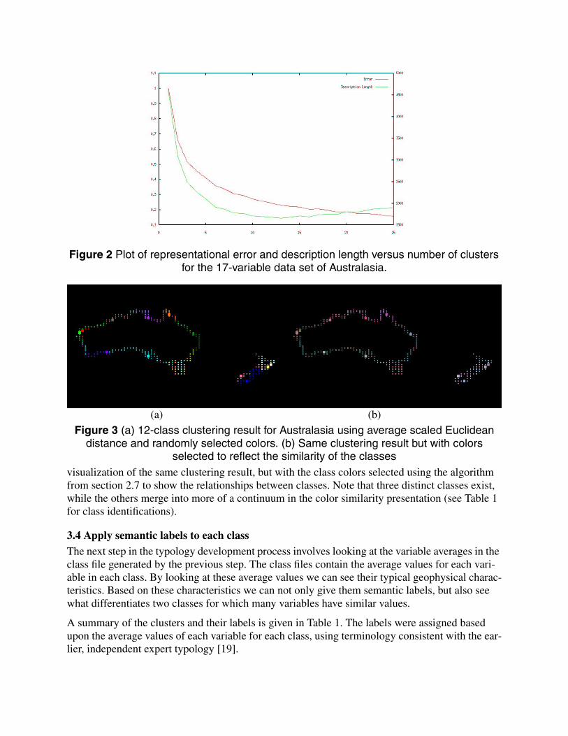
visualization of the same clustering result, but with the class colors selected using the algorithmfrom section 2.7 to show the relationships between classes. Note that three distinct classes exist,while the others merge into more of a continuum in the color similarity presentation (see Table 1for class identifications).

3.4 Apply semantic labels to each classThe next step in the typology development process involves looking at the variable averages in theclass file generated by the previous step. The class files contain the average values for each vari-able in each class. By looking at these average values we can see their typical geophysical charac-teristics. Based on these characteristics we can not only give them semantic labels, but also seewhat differentiates two classes for which many variables have similar values.

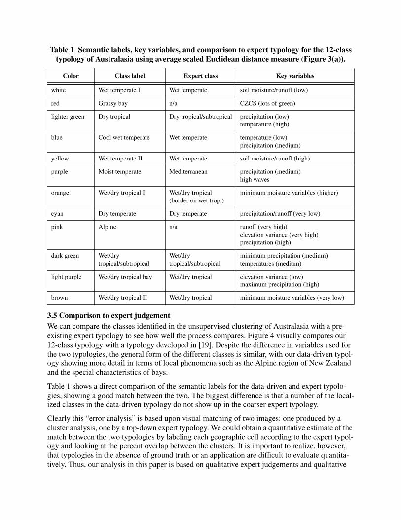
A summary of the clusters and their labels is given in Table 1. The labels were assigned basedupon the average values of each variable for each class, using terminology consistent with the ear-lier, independent expert typology [19].

Figure 2 Plot of representational error and description length versus number of clustersfor the 17-variable data set of Australasia.

(a) (b)

Figure 3 (a) 12-class clustering result for Australasia using average scaled Euclideandistance and randomly selected colors. (b) Same clustering result but with colors

selected to reflect the similarity of the classes

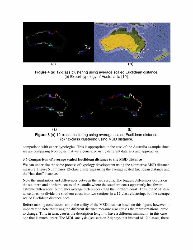
3.5 Comparison to expert judgementWe can compare the classes identified in the unsupervised clustering of Australasia with a pre-existing expert typology to see how well the process compares. Figure 4 visually compares our12-class typology with a typology developed in [19]. Despite the difference in variables used forthe two typologies, the general form of the different classes is similar, with our data-driven typol-ogy showing more detail in terms of local phenomena such as the Alpine region of New Zealandand the special characteristics of bays.

Table 1 shows a direct comparison of the semantic labels for the data-driven and expert typolo-gies, showing a good match between the two. The biggest difference is that a number of the local-ized classes in the data-driven typology do not show up in the coarser expert typology.

Clearly this “error analysis” is based upon visual matching of two images: one produced by acluster analysis, one by a top-down expert typology. We could obtain a quantitative estimate of thematch between the two typologies by labeling each geographic cell according to the expert typol-ogy and looking at the percent overlap between the clusters. It is important to realize, however,that typologies in the absence of ground truth or an application are difficult to evaluate quantita-tively. Thus, our analysis in this paper is based on qualitative expert judgements and qualitative

Table 1 Semantic labels, key variables, and comparison to expert typology for the 12-classtypology of Australasia using average scaled Euclidean distance measure (Figure 3(a)).

Color Class label Expert class Key variables

white Wet temperate I Wet temperate soil moisture/runoff (low)

red Grassy bay n/a CZCS (lots of green)

lighter green Dry tropical Dry tropical/subtropical precipitation (low)temperature (high)

blue Cool wet temperate Wet temperate temperature (low)precipitation (medium)

yellow Wet temperate II Wet temperate soil moisture/runoff (high)

purple Moist temperate Mediterranean precipitation (medium)high waves

orange Wet/dry tropical I Wet/dry tropical(border on wet trop.)

minimum moisture variables (higher)

cyan Dry temperate Dry temperate precipitation/runoff (very low)

pink Alpine n/a runoff (very high)elevation variance (very high)precipitation (high)

dark green Wet/drytropical/subtropical

Wet/drytropical/subtropical

minimum precipitation (medium)temperatures (medium)

light purple Wet/dry tropical bay Wet/dry tropical elevation variance (low)maximum precipitation (high)

brown Wet/dry tropical II Wet/dry tropical minimum moisture variables (very low)

comparison with expert typologies. This is appropriate in the case of the Australia example sincewe are comparing typologies that were generated using different data sets and approaches.

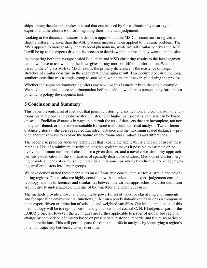
3.6 Comparison of average scaled Euclidean distance to the MSD distanceWe can undertake the same process of typology development using the alternative MSD distancemeasure. Figure 5 compares 12-class clusterings using the average scaled Euclidean distance andthe Hausdorff distance.

Note the similarities and differences between the two results. The biggest differences occurs onthe southern and northern coasts of Australia where the southern coast apparently has fewerextreme differences (but higher average differences) than the northern coast. Thus, the MSD dis-tance does not divide the southern coast into two sections in a 12-class clustering, but the averagescaled Euclidean distance does.

Before making conclusions about the utility of the MSD distance based on this figure, however, itimportant to note that using the different distance measure also causes the representational errorto change. This, in turn, causes the description length to have a different minimum--in this caseone that is much larger. The MDL analysis (see section 2.4) says that instead of 12 classes, there

Figure 4 (a) 12-class clustering using average scaled Euclidean distance.(b) Expert typology of Australasia [19].

(a) (b)

Figure 5 (a) 12-class clustering using average scaled Euclidean distance.(b) 12-class clustering using MSD distance.

(a) (b)

should be more like 24-40. In other words, when you are looking at extremes rather than averages,there are more extremes to be considered.

Figure 6(a) shows an example of a 24 class clustering result using the ASE distance measure. Fig-ure 6(b) shows a 24 class clustering result using the MSD distance measure. In the MSD plot, theplaces that significantly increased in complexity were the southern coast (one class became four),New Zealand (3 classes became 6), and the grassy bay cluster (one became three). These threeregions account for 8 of the 12 new classes, and highlight where significant localized changes ingeographic variables are taking place.

The other subtle difference between the two plots is that the MSD appears to generate more con-tiguous regions and pick up on more details than the ASE.

3.7 Segmentation and merging to generate class descriptionsAs a final comparison, we applied the region growing and merging technique to the same data set.For the local parameter threshold--how similar a neighboring point must be--we used 1.0 standarddeviation. For the global parameter threshold--how similar a point must be to the original seedpoint--we used 1.22 standard deviations. Points had to be within two degrees of one another to beconsidered adjacent, and the distance measure was the average scaled Euclidean distance.

The resulting segmentation contained 170 different contiguous regions: three significant regionsand 167 1-3 point regions. Applying the merge technique to this set of regions, the graph ofdescription length versus number of clusters gives us a guide as to when to stop merging. Figure 7shows this graph, which bottoms out between 16-28 classes. In Figure 8 we show the 28 classresult, which appears to highlight a number of localized phenomena, similar to the MSD distance.Note that the localized phenomena each tend to occupy a different class, however, since the seg-mentation process requires data points to be contiguous.

4 Discussion and Future Directions

The first question we need to answer is whether the typology development process outlined abovegives us something useful. From the Australasia example, the answer seems to be that it does pro-duce a reasonable set of classes. The results show broad agreement with the previous expert typol-

Figure 6 (a) Clustering result for 24 classes using the ASE distance. (b) Clustering resultfor 24 classes using the MSD distance.

(a) (b)

ogy. Furthermore, they highlight localized phenomena that do not show up in the expert version,but nevertheless exist in the data. Note that we obtained these results despite heterogeneous vari-ables with some missing data, indicating that the distance measures we used are appropriate forthe task.

The primary real benefit of the data-driven methodology is that it gives us a quantitative, consis-tent, and objective way to compare classes across both space and time. Thus, this approach can beused not only to compare coastlines across the world within a temporally fixed data set, but canalso be used to compare how coastlines change based on actual or predicted climate change.

A second real benefit of using the bottom-up expert guided approach is in the time saving aspectof the process. A group of experts that included the authors was able to develop the complete Aus-tralasia typology with the span of an hour. This was largely because of the tools we developed forautomating the process--MDL analysis, clustering, and visualization.

A third real benefit of this approach is its utility for integration of data and communication aboutresults across disciplinary boundaries. Human dimension variables and physical variables that areboth environmental forcing functions can be effectively combined, even though their mechanismsof operation are very different. The visual presentation of results, and the specification of relation-

Figure 7 Description length versus number of clusters during merging (mergeprocess goes right to left from 170 down to 1)

Figure 8 (a) 170 region result of segmentation process.(b) 28 region result of segmentation followed by merging.

(a) (b)

ships among the clusters, makes it a tool that can be used by for calibration by a variety ofexperts--and therefore a tool for integrating their individual judgments.

Looking at the distance measures in detail, it appears that the MSD distance measure gives usslightly different classes than the ASE distance measure when applied to the same problem. TheMSD appears to more readily identify local phenomena, while overall similarity drives the ASE.It will be up to the experts driving the process to decide which approach they want to emphasize.

In comparing both the average scaled Euclidean and MSD clustering results to the local segmen-tation, we have to ask whether the latter gives us any more or different information. When com-pared to the 24 class ASE or MSD results, the primary difference is the existence of longerstretches of similar coastline in the segmentation/merging result. This occurred because the longsouthern coastline was a single group to start with, which meant it never split during the process.

Whether the segmentation/merging offers any new insights is unclear from the single example.We need to undertake more experimentation before deciding whether to pursue it any further as apotential typology development tool.

5 Conclusion and Summary

This paper presents a set of methods that permit clustering, classification, and comparison of envi-ronments at regional and global scales. Clustering of high-dimensionality data sets can be basedon scaled Euclidian distances in ways that permit the use of data sets that are incomplete, not nor-mally distributed, or otherwise unsuitable for more traditional statistical analysis. Two differentdistance criteria -- the average scaled Euclidean distance and the maximum scaled distance -- pro-vide alternative ways to explore the nature of environmental similarities and differences.

The paper also presents ancillary techniques that expand the applicability and ease of use of thesemethods. Use of a minimum description length algorithm makes it possible to estimate objec-tively the optimum number of clusters for a given data set, and a novel color-similarity approachpermits visualization of the similarities of spatially distributed clusters. Methods of cluster merg-ing provide a means of establishing hierarchical relationships among the clusters, and of aggregat-ing smaller clusters into larger groups.

We have demonstrated these techniques on a 17-variable coastal data set for Australia and neigh-boring regions. The results are highly consistent with an independent expert-judgement coastaltypology, and the differences and similarities between the various approaches to cluster definitionare intuitively understandable in terms of the variables and techniques used.

The methods provide a novel and potentially powerful set of tools for classifying environmentsand for upscaling environmental functions, either on a purely data-driven basis or as a componentin an expert-driven examination of selected and weighted variables. Our initial application of thismethodology will be to regionalization and globalization of coastal C, N, P budgets as part of theLOICZ projects. However, the techniques are further applicable to issues of global and regionalchange by comparison of clusters based on present data, historical records, and future scenarios ormodel predictions. This will permit space-for-time trade-offs in analysis by identifying a region’spotential trajectory between clusters over time.

AcknowledgementsThe authors would like to thank LOICZ for their support of the typology project and the workdescribed herein. We would also like to thank AAAS for the Earth Systems Science Conference in1997 in South Dakota which brought together scientists from a variety of disciplines--includingthe authors--and launched this approach to coastline typology development.

References[1] Anderberg, MR (1973) Cluster Analysis for Applications, Academic Press, New York.

[2] Ankerst, M, Berchtold, S, and Keim, D (1998) ‘‘Similarity clustering of dimensions for anenhanced visualization of multidimensional data,’’ Proc. Information Visualization ’98,pp. 52-60, October, 1998.

[3] Backer, E (1995) Computer-Assisted Reasoning in Cluster Analysis, Prentice Hall, Engle-wood Cliffs, NJ.

[4] Dyer, KR, Christie, MC, and Wright, EW (2000) “The classification of intertidal mud-flats”, Continental Shelf Research, Vol. 20, no. 10-11, July, pp. 1039-1060.

[5] Gordon, J, DC et al., (1995) LOICZ Biogeochemical Modelling Guidelines, LOICZReports & Studies No. 5. LOICZ, Texel, The Netherlands, vi + 96 pp.

[6] Harff, J and Davis, JC (1990) “Regionalization in Geology by Multivariate Classification”,Mathematical Geology, Vol. 22, No. 5, pp.573-588.

[7] Hartigan, JA and Wong, MA (1979) "A K-Means Clustering Algorithm". Applied Statis-tics 28: 100--108.

[8] Huttenlocher, DP, Klanderman, GA, and Rucklidge, WJ (1993) “Comparing ImagesUsing the Hausdorff Distance”, PAMI(15), No. 9, pp. 850-863.

[9] IPCC Data Distribution Centre for Climate Change and Related Scenarios for ImpactsAssessment; CD-ROM, Version 1.0, April 1999.

[10] Lankford, R. (1977) "Coastal lagoons of Mexico: their origin and classification", pp. 182-215 in M. Wiley (ed.) Estuarine Processes, Academic, New York.

[11] LOICZ typology data set, http://www.kellia.nioz.nl/loicz/typo.htm

[12] MacQueen, J (1965) "On convergence of k-means and partitions with minimum averagevariance," Ann. Math. Statist., 36, p. 1084, 1965.

[13] Maktav, D (1985) “The study of the natural geographic differences in the coastal areas ofwater covered parts of Marmara Region in Turkey with the help of Landsat-4 MSS datausing an unsupervised classification algorithm with Euclidean distance”, Eleventh Inter-national Symposium on Machine Processing of Remotely Sensed Data, West Lafayette,IN, USA; pp.122-7.

[14] Pernetta, JC and Milliman, JD (Editors) (1995) Land-Ocean Interactions in the CoastalZone: Implementation Plan. IGBP Report No. 33. IGBP, Stockholm, 215 pp.

[15] Piramuthu, S (1999) “The Hausdorff distance measure for feature selection in learningapplications”, Proceedings of the 32nd Annual Hawaii International Conference on Sys-tems Sciences. IEEE Computing Society.

[16] Prakash, HNS., Kumar, SR, Nagabhushan, P, Gowda, KC (1996) “Modified divisive clus-tering useful for quantitative analysis of remotely sensed data”, IGARSS ’96: 1996 Inter-national Geoscience and Remote Sensing Symposium, IEEE, New York, NY, USA,pp.1858-60 vol.3.

[17] Rabiner, L, and Juang, B-H (1993) Fundamentals of Speech Recognition, Prentice-Hall,Englewood Cliffs, NJ.

[18] Rissanen, J (1989) Stochastic Complexity in Statistical Inquiry, World Scientific Publish-ing Co. Ptc. Ltd., Singapore.

[19] Smith, SV, and Crossland, C J (1999) Austalasian Estuarine Systems: Carbon, Nitrogenand Phosphorus Fluxes, LOICZ Reports & Studies No. 12, ii + 182 pp. LOICZ, Texel,The Netherlands.

[20] Smith, SV, and Ibarra-Obando, S, Boudreau, PR, and Camacho-Ibar, VF (1997) Compari-son of Carbon, Nitrogen and Phosphorous Fluxes in Mexican Coastal Lagoons, LOICZCore Project of IGBP, Texel, The Netherlands.