COARSE-GRADIENT LANGEVIN ALGORITHMS FOR DYNAMICDATA INTEGRATION AND UNCERTAINTY QUANTIFICATION

P. DOSTERT∗, Y. EFENDIEV† , T.Y. HOU‡ , AND W. LUO§

Abstract.

The main goal of this paper is to design an efficient sampling technique for dynamic data integra-tion using the Langevin algorithms. Based on a coarse-scale model of the problem, we compute theproposals of the Langevin algorithms using the coarse-scale gradient of the target distribution. Toguarantee a correct and efficient sampling, each proposal is first tested by a Metropolis acceptance-rejection step with a coarse-scale distribution. If the proposal is accepted in the first stage, thena fine-scale simulation is performed at the second stage to determine the acceptance probability.Comparing with the direct Langevin algorithm, the new method generates a modified Markov chainby incorporating the coarse-scale information of the problem. Under some mild technical condi-tions we prove that the modified Markov chain converges to the correct posterior distribution. Wewould like to note that the coarse-scale models used in the simulations need to be inexpensive, butnot necessarily very accurate, as our analysis and numerical simulations demonstrate. We presentnumerical examples for sampling permeability fields using two-point geostatistics. Karhunen-Loeveexpansion is used to represent the realizations of the permeability field conditioned to the dynamicdata, such as the production data, as well as the static data. The numerical examples show that thecoarse-gradient Langevin algorithms are much faster than the direct Langevin algorithms but havesimilar acceptance rates.

1. Introduction. Uncertainties in the detailed description of reservoir lithofa-cies, porosity, and permeability are major contributors to uncertainty in reservoir per-formance forecasting. Making decisions in reservoir management requires a methodfor quantifying uncertainty. Large uncertainties in reservoirs can greatly affect theproduction and decision making on well drilling. Better decisions can be made byreducing the uncertainty. Thus, quantifying and reducing the uncertainty is an im-portant and challenging problem in subsurface modeling. Additional dynamic data,such as the production data, can be used in achieving more accurate predictions. Theprevious findings show that dynamic data can be used to improve the predictionsand reduce the uncertainty. Therefore, to predict future reservoir performance, thereservoir properties, such as porosity and permeability, need to be conditioned todynamic data. In general it is difficult to calculate this posterior probability distri-bution because the process of predicting flow and transport in petroleum reservoirsis nonlinear. Instead, we estimate this probability distribution from the outcomes offlow predictions for a large number of realizations of the reservoir. It is essential thatthe permeability (and porosity) realizations adequately reflect the uncertainty in thereservoir properties, i.e., we correctly sample this probability distribution.

The prediction of permeability fields based on dynamic data is a challenging prob-lem because permeability fields are typically defined on a large number of grid blocks.The Markov chain Monte Carlo (MCMC) method and its modifications have beenused previously to sample the posterior distribution of the permeability field. Oliveret al. [21, 22] proposed the randomized maximum likelihood method, which generatesunconditional realizations of the production and permeability data and then solvesa deterministic gradient-based inverse problem. The solution of this minimizationproblem is taken as a proposal and accepted with probability one because the rig-

∗Department of Mathematics, Texas A&M University, College Station, TX 77843-3368†Department of Mathematics, Texas A&M University, College Station, TX 77843-3368‡Applied Mathematics, Caltech, Pasadena, CA 91125. Corresponding Author§Applied Mathematics, Caltech, Pasadena, CA 91125

1

orous acceptance probability is very difficult to estimate. In addition to the need ofsolving a gradient-based inverse problem, this method does not guarantee a propersampling of the posterior distribution. Developing efficient and rigorous MCMC cal-culations with high acceptance rates remains a challenging problem.

In this paper, we employ the Langevin algorithms within the context of MCMCmethods for sampling the permeability field. Langevin algorithms provide efficientsampling techniques because they use the gradient information of the target distribu-tions. However, the direct Langevin algorithm is very expensive because it requiresthe computation of the gradients with fine-scale simulations. Based on a coarse-scalemodel of the problem, we propose an approach where the gradients are computed withinexpensive coarse-scale simulation. These coarse-scale gradients may not be very ac-curate and, for this reason, the computed results are first tested with coarse-scaledistributions. If the result is accepted at the first stage, then a fine-scale simulationis performed at the second stage to determine the acceptance probability. The firststage of the method modifies the Markov chain generated by the direct Langevin al-gorithms. We can show that the modified Markov chain satisfies the detailed balancecondition for the correct distribution. Moreover, we point out that the chain is ergodicand converges to the correct posterior distribution under some technical assumptions.The validity of the assumptions for our application is also discussed in the paper

For sampling the permeability fields in two-phase flows, we use a coarse-scalemodel based on multiscale finite element methods. The multiscale finite elementmethods are used to construct coarse-scale velocity fields which are further used tosolve the transport equation on the coarse-grid. The multiscale basis functions arenot updated throughout the simulation, which provides an inexpensive coarse-scalemethodology. In this respect, the multiscale finite element methods are conceptuallysimilar to the single-phase flow upscaling methods (see e.g., [3, 5]), where the mainidea is to upscale the underlying fine-scale permeability field. These types of upscalingmethods are not very accurate because the subgrid effects of transport are neglected.We would like to note that upscaled models are used in MCMC simulations in pre-vious findings. In a pioneering work ([12]), Glimm and Sharp employed error modelsbetween coarse- and fine-scale simulations to quantify the uncertainty.

Numerical results for sampling permeability fields using two-point geostatisticsare presented in the paper. Using the Karhunen-Loeve expansion, we can representthe high dimensional permeability field by a small number of parameters. Further-more, the static data (the values of permeability fields at some sparse locations) can beeasily incorporated into the Karhunen-Loeve expansion to further reduce the dimen-sion of the parameter space. Imposing the values of the permeability at some locationsrestricts the parameter space to a subspace (hyperplane). Numerical results are pre-sented for both single-phase and two-phase flows. In all the simulations, we showthat the gradients of the target distribution computed using coarse-scale simulationsprovide accurate approximations of the actual fine-scale gradients. Furthermore, wepresent the uncertainty assessment of the production data based on sampled perme-ability fields. Our numerical results show that the uncertainty spread is much largerif no dynamic data information is used. However, the uncertainty spread decreases ifmore information is incorporated into the simulations.

The paper is organized as follows. In the next section, we briefly describe themodel equations and their upscaling. Section 3 is devoted to the analysis of theLangevin MCMC method and its relevance to our particular application. Numericalresults are presented in Section 4.

2

2. Fine and coarse models. In this section we briefly introduce a coarse-scalemodel used in the simulations. We consider two-phase flows in a reservoir (denotedby Ω) under the assumption that the displacement is dominated by viscous effects;i.e., we neglect the effects of gravity, compressibility, and capillary pressure. Porositywill be considered to be constant. The two phases will be referred to as water and oil,designated by subscripts w and o, respectively. We write Darcy’s law for each phaseas follows:

vj = −krj(S)

µj

k · ∇p, (2.1)

where vj is the phase velocity, k is the permeability tensor, krj is the relative per-meability to phase j (j = o, w), S is the water saturation (volume fraction) and pis pressure. Throughout the paper, we will assume that the permeability tensor isdiagonal k = kI, where k is a scalar and I is the unit tensor. In this work, a singleset of relative permeability curves is used. Combining Darcy’s law with a statementof conservation of mass allows us to express the governing equations in terms of theso-called pressure and saturation equations:

∇ · (λ(S)k∇p) = h, (2.2)

∂S

∂t+ v · ∇f(S) = 0, (2.3)

where λ is the total mobility, h is the source term, f(S) is the flux function, and v isthe total velocity, which are respectively given by:

λ(S) =krw(S)

µw

+kro(S)

µo

, (2.4)

f(S) =krw(S)/µw

krw(S)/µw + kro(S)/µo

, (2.5)

v = vw + vo = −λ(S)k · ∇p. (2.6)

The above descriptions are referred to as the fine model of the two-phase flow problem.For the single-phase flow, krw(S) = S and kro(S) = 1 − S.

In most upscaling procedures, the coarse-scale pressure equation is of the sameform as the fine-scale equation (2.2) but with an equivalent grid block permeabilitytensor replacing the fine-scale permeability field (see e.g., [5]). In this work, theproposed coarse-scale model consists of the upscaling of the pressure equation (2.2) inorder to obtain the velocity field on the coarse-grid and use it in (2.3) to resolve thesaturation on the coarse-grid. The pressure equation is scaled up using a multiscalefinite volume method. The multiscale finite volume method is similar to the recentlyintroduced multiscale finite element methods. The details of the method are presentedin Appendix A. Using the multiscale finite volume method, we obtain the coarse-scalevelocity field, which is used in solving the saturation equation on the coarse-grid. Sinceno subgrid modeling is performed for the saturation equation, this upscaling procedureintroduces errors. In Figure 2.1, we plot a typical fractional flow comparison betweenfine- and coarse-scale models. Fractional flow F (t) (denoted simply by F in further

3

0 0.2 0.4 0.6 0.8 1 1.2 1.4 1.6 1.8 20

0.1

0.2

0.3

0.4

0.5

0.6

0.7

0.8

0.9

1

PVI

F

finecoarse

Fig. 2.1. Typical fine and coarse scale fractional flows

discussion) is defined as the fraction of oil in the produced fluid and is given by qo/qt,where qt = qo + qw, with qo and qw the flow rates of oil and water at the productionedge of the model. More specifically,

F (t) = 1 −∫

∂Ωout f(S)vndl∫

∂Ωout vndl,

where ∂Ωout is outflow boundaries and vn is the normal velocity field. In Figure 2.1the fractional flows are plotted against the dimensionless time Pore Volume Injected

(PVI). The PVI at time T is defined as 1Vp

∫ T

0qt(τ)dτ , with Vp the total pore volume

of the system. PVI provides the dimensionless time for the displacement.

3. Langevin algorithm using coarse-scale models.

3.1. Problem setting. The problem under consideration consists of samplingthe permeability field given fractional flow measurements. Typically, the prior infor-mation about the permeability field consists of its covariance matrix and the values ofthe permeability at some sparse locations. Since the fractional flow is an integratedresponse, the map from the permeability field to the fractional flow is not one-to-one.Hence this problem is ill-posed in the sense that there exist many different permeabil-ity realizations for the given production data.

From the probabilistic point of view, this problem can be regarded as conditioningthe permeability fields to the fractional flow data with measurement errors. Conse-quently, our goal is to sample from the conditional distribution P (k|F ), where k isthe fine-scale permeability field and F is the fractional flow data. Using the Bayesformula we can write

P (k|F ) ∝ P (F |k)P (k). (3.1)

In the above formula, P (k) is the unconditioned (prior) distribution of the permeabil-ity field. In practice, the measured fractional flow contains measurement errors. Inthis paper, we assume that the measurement error satisfies a Gaussian distribution,thus, the likelihood function P (F |k) takes the form

P (F |k) ∝ exp(

−‖F − Fk‖2

σ2f

)

, (3.2)

4

where F is the reference fractional flow, Fk is the fractional flow for the permeabilityfield k, and σf is the measurement precision. In practice, Fk is computed by solvingthe nonlinear PDE system (2.1)-(2.3) for the given k on the fine-grid. Since both Fand Fk are functions of time (denoted by t), the norm ‖F −Fk‖2 is defined as the L2

norm

‖F − Fk‖2 =

∫ T

0

[F (t) − Fk(t)]2dt.

Denote the sampling target distribution as

π(k) = P (k|F ) ∝ exp(

−‖F − Fk‖2

σ2f

)

P (k). (3.3)

Since different permeability fields may produce the same fractional flow curve, thedistribution π(k) is a function of k with multiple local maxima. Sampling from thedistribution π(k) can be accomplished by the MCMC method. For a given proposaldistribution q(y|x), the Metropolis-Hasting MCMC algorithm (see, e.g., [23], page233) consists of the following steps.

Algorithm I (Metropolis-Hasting MCMC, Robert and Casella [23])• Step 1. At kn generate Y from q(Y |kn).• Step 2. Accept Y as a sample with probability

p(kn, Y ) = min

(

1,q(kn|Y )π(Y )

q(Y |kn)π(kn)

)

, (3.4)

i.e. take kn+1 = Y with probability p(kn, Y ), and kn+1 = kn with probability1 − p(kn, Y ).

The MCMC algorithm generates a Markov chain kn whose stationary distributionis π(k). A remaining question is how to choose an efficient proposal distributionq(Y |kn).

An important type of proposal distribution can be derived from the Langevindiffusion, as proposed by Grenander and Miller [13]. The Langevin diffusion is definedby the stochastic differential equation

dk(τ) =1

2∇ log π(k(τ))dτ + dWτ , (3.5)

where Wτ is the standard Brownian motion vector with independent components. Itcan be shown that the diffusion process k(τ) has π(k) as its stationary distribution.The actual implementation of the Langevin diffusion requires a discretization of theequation (3.5),

kn+1 = kn +∆τ

2∇ log π(kn) +

√∆τǫn,

where ǫn are independent standard normal distributions. However, the discrete solu-tion kn can have vastly different asymptotic behavior from the continuous diffusionprocess k(τ) [23]. In general, the discrete solution kn does not necessarily have π(k)as its stationary distribution. Instead of taking kn as samples directly, we use themas test proposals for Algorithm I. The samples will be further tested and corrected by

5

the Metropolis acceptance-rejection step (3.4). Consequently, we choose the proposalgenerator q(Y |kn) in Algorithm I as

Y = kn +∆τ

2∇ log π(kn) +

√∆τǫn. (3.6)

Since ǫn are independent Gaussian vectors, the transition distribution of the proposalgenerator (3.6) is

q(Y |kn) ∝ exp

(

−‖Y − kn − ∆τ2 ∇ log π(kn)‖2

2∆τ

)

,

q(kn|Y ) ∝ exp

(

−‖kn − Y − ∆τ2 ∇ log π(Y )‖2

2∆τ

)

.

(3.7)

The scheme (3.6) can be regarded as a problem-adapted random walk. The gra-dient information of the target distribution is included to enforce a biased randomwalk. The use of the gradient information in inverse problems for subsurface char-acterization is not new. In their original work, Oliver et al [21, 22] developed therandomized maximum likelihood method, which uses the gradient information of thetarget distribution. This approach uses unconditional realizations of the productionand permeability data and solves a deterministic gradient-based minimization prob-lem. The solution of this minimization problem is taken as a proposal and is acceptedwith probability one, since the acceptance probability is very difficult to estimate.In addition to the need of solving a gradient-based inverse problem, this methoddoes not guarantee a proper sampling of the posterior distribution. Thus, develop-ing efficient and rigorous MCMC calculations with high acceptance rates remains achallenging problem. Though the Langevin formula (3.6) resembles the randomizedmaximum likelihood method, it is more efficient and rigorous, and one can computethe acceptance probability easily. The Langevin algorithms also allow us to achievehigh acceptance rates. However, computing the gradients of the target distributionis very expensive. In this paper, we propose to use the coarse-scale solutions in thecomputation of the gradients to speed up the Langevin algorithms.

3.2. Langevin MCMC method using coarse-scale models. The majorcomputational cost of Algorithm I is to compute the value of the target distribu-tion π(k) at different permeabilities. Since the map between the permeability k andthe fractional flow Fk is governed by the PDE system (2.1)-(2.3), there is no explicitformula for the target distribution π(k). To compute the function π(k), we need tosolve the nonlinear PDE system (2.1)-(2.3) on the fine scale for the given k. Forthe same reason, we need to compute the gradient of π(k) in (3.6) numerically (byfinite differences), which involves solving the nonlinear PDE system (2.1)-(2.3) multi-ple times. To compute the acceptance probability (3.4), the PDE system (2.1)-(2.3)needs to be solved one more time. As a result, the direct (full) MCMC simulationswith Langevin samples are prohibitively expensive.

To bypass the above difficulties, we design a coarse-grid Langevin MCMC algo-rithm where most of the fine scale computations are replaced by the coarse scale ones.Based on a coarse-grid model of the distribution π(k), we first generate samples from(3.6) using the coarse-scale gradient of π(k), which only requires solving the PDEsystem (2.1)-(2.3) on the coarse-grid. Then we further filter the proposals by an ad-ditional Metropolis acceptance-rejection test on the coarse-grid. If the sample does

6

not pass the coarse-grid test, the sample is rejected and no further fine-scale test isnecessary. The argument for this procedure is that if a proposal is not accepted bythe coarse-grid test, then it is unlikely to be accepted by the fine scale test either.By eliminating most of the “unlikely” proposals with cheap coarse-scale tests, we canavoid wasting CPU time simulating the rejected samples on the fine-scale.

To model π(k) on the coarse-scale, we define a coarse-grid map F ∗k between the

permeability field k and the fractional flow F . The map F ∗k is determined by solving

the PDE system (2.1)-(2.3) on a coarse-grid. Consequently, the target distributionπ(k) can be approximated by

π∗(k) ∝ exp

(

−‖F − F ∗k ‖2

σ2c

)

P (k), (3.8)

where σc is the measurement precision on the coarse-grid, and should be slightly largerthan σf . Then the Langevin samples are generated from (3.6) using the coarse-gridgradient of the target distribution

Y = kn +∆τ

2∇ log π∗(kn) +

√∆τǫn. (3.9)

The transition distribution of the coarse-grid proposal (3.9) is

q∗(Y |kn) ∝ exp

(

−‖Y − kn − ∆τ2 ∇ log π∗(kn)‖2

2∆τ

)

,

q∗(kn|Y ) ∝ exp

(

−‖kn − Y − ∆τ2 ∇ log π∗(Y )‖2

2∆τ

)

.

(3.10)

To compute the gradient of π∗(kn) numerically, we only need to solve the PDE system(2.1)-(2.3) on the coarse-grid. The coarse-scale distribution π∗(k) serves as a regular-ization of the original fine-scale distribution π(k). By replacing the fine-scale gradientwith the coarse-scale gradient, we can reduce the computational cost dramatically butstill direct the proposals to regions with larger probabilities.

Because of the high dimension of the problem and the discretization errors, mostproposals generated by the Langevin algorithms (both (3.6) and (3.9)) will be rejectedby the Metropolis acceptance-rejection test (3.4). To avoid wasting expensive fine-scale computations on unlikely acceptable samples, we further filter the Langevinproposals by the coarse-scale acceptance criteria

g (kn, Y ) = min

(

1,q∗ (kn|Y )π∗(Y )

q∗(Y |kn)π∗ (kn)

)

,

where π∗(k) is the coarse-scale target distribution (3.8), q∗(Y |kn) and q∗(kn|Y ) arethe coarse-scale proposal distributions given by (3.10). Combining all the discussionabove, we have the following revised MCMC algorithm.

Algorithm II (Preconditioned coarse-gradient Langevin algorithm)• Step 1. At kn, generate a trial proposal Y from the coarse Langevin algorithm

(3.9).• Step 2. Take the proposal k as

k =

Y with probability g(kn, Y ),kn with probability 1 − g(kn, Y ),

7

where

g(kn, Y ) = min

(

1,q∗(kn|Y )π∗(Y )

q∗(Y |kn)π∗(kn)

)

.

Therefore, the proposal k is generated from the effective instrumental distri-bution

Q(k|kn) = g(kn, k)q∗(k|kn) +

(

1 −∫

g(kn, k)q∗(k|kn)dk

)

δkn(k). (3.11)

• Step 3. Accept k as a sample with probability

ρ(kn, k) = min

(

1,Q(kn|k)π(k)

Q(k|kn)π(kn)

)

, (3.12)

i.e., kn+1 = k with probability ρ(kn, k), and kn+1 = kn with probability1 − ρ(kn, k).

The step 2 screens the trial proposal Y by the coarse-grid distribution before passingit to the fine-scale test. The filtering process changes the proposal distribution ofthe algorithm from q∗(Y |kn) to Q(k|kn) and serves as a preconditioner to the MCMCmethod. This is why we call it the preconditioned coarse-gradient Langevin algorithm.We note that testing proposals by approximate target distributions is not a very newidea. Similar strategies have been developed previously in [17, 2].

Note that there is no need to compute Q(k|kn) and Q(kn|k) in (3.12) by formula(3.11). The acceptance probability (3.12) can be simplified as

ρ(kn, k) = min

(

1,π(k)π∗(kn)

π(kn)π∗(k)

)

. (3.13)

In fact, this is obviously true for k = kn since ρ(kn, kn) ≡ 1. For k 6= kn,

Q(kn|k) = g(k, kn)q(kn|k) =1

π∗(k)min

(

q(kn|k)π∗(k), q(k|kn)π∗(kn))

=q(k|kn)π∗(kn)

π∗(k)g(kn, k) =

π∗(kn)

π∗(k)Q(k|kn).

Substituting the above formula into (3.12), we immediately get (3.13).In Algorithm II, the proposals generated by (3.9) are screened by the coarse-scale

acceptance-rejection test to reduce the number of unnecessary fine-scale simulations.One can skip that preconditioning step and get the following algorithm.

Algorithm III (Coarse-gradient Langevin algorithm)• Step 1. At kn, generate a trial proposal Y from the coarse Langevin algorithm

(3.9).• Step 2. Accept Y as a sample with probability

ρ(kn, Y ) = min

(

1,q∗(kn|Y )π(Y )

q∗(Y |kn)π(kn)

)

, (3.14)

i.e. kn+1 = Y with probability ρ(kn, Y ), and kn+1 = kn with probability1 − ρ(kn, Y ).

8

We will demonstrate numerically that Algorithm II is indeed more efficient thanAlgorithm III.

In a previous work [10], we studied preconditioning the MCMC algorithms bycoarse-scale models, where the independent sampler and random walk sampler areused as the instrumental distribution. In this paper, our goal is to show that onecan use coarse-scale models in Langevin algorithms. In particular, we can use coarse-scale gradients instead of fine-scale gradients in these algorithms. Our numericalexperiments show that the coarse-scale distribution somewhat regularizes (smooths)the fine-scale distribution, which allows us to take larger time steps in the Langevinalgorithm (3.9). In addition, we employ the preconditioning technique from [10] toincrease the acceptance rate of the coarse-gradient Langevin algorithms.

3.3. Analysis of the coarse-gradient Langevin algorithms. In this section,we will briefly discuss the convergence property of the preconditioned coarse-gridLangevin algorithm. Denote

E =

k; π(k) > 0

,

E∗ =

k; π∗(k) > 0

,

D =

k; q∗(k|kn) > 0 for any kn ∈ E

.

(3.15)

The set E is the support of the posterior (target) distribution π(k). E contains allthe permeability fields k which have a positive probability of being accepted as asample. Similarly, E∗ is the support of the coarse-scale distribution π∗(k), whichcontains all the k acceptable by the the coarse-scale test. D is the set of all possibleproposals which can be generated by the Langevin distribution q∗(k|kn). To makethe coarse-gradient Langevin MCMC methods sample properly, the conditions E ⊆ Dand E ⊆ E∗ must hold (up to a zero measure set) simultaneously. If one of theseconditions is violated, say, E 6⊆ E∗, then there will exist a subset A ⊂ (E \ E∗) suchthat

π(A) =

∫

A

π(k)dk > 0 and π∗(A) =

∫

A

π∗(k)dk = 0,

which means no element of A can pass the coarse-scale test and A will never be visitedby the Markov chain kn. For Langevin algorithms, E ⊂ D is always satisfied sinceD is the whole space. By choosing the parameter σc in π∗(k) properly, the conditionE ⊂ E∗ can also be satisfied. A typical choice would be σc ≈ σf . More discussions onthe choice of σc can be found in [10], where a two-stage MCMC algorithm is discussed.

Denote by K the transition kernel of the Markov chain kn generated by Algo-rithm II. Since its effective instrumental proposal is Q(k|kn), the transition kernel Khas the form

K(kn, k) = ρ(kn, k)Q(k|kn), k 6= kn,

K(kn, kn) = 1 −∫

k 6=knρ(kn, k)Q(k|kn)dk.

(3.16)

That is, the transition kernel K(kn, ·) is continuous when k 6= kn and has a positiveprobability at the point k = kn. First we show that K(kn, k) satisfies the detailedbalance condition, that is

π(kn)K(kn, k) = π(k)K(k, kn) (3.17)

9

for all k, kn. The equality is obvious when k = kn. If k 6= kn, then

π(kn)K(kn, k) = π(kn)ρ(kn, k)Q(k|kn) = min(

Q(k|kn)π(kn), Q(kn|k)π(k))

=min

(

Q(k|kn)π(kn)

Q(kn|k)π(k), 1

)

Q(kn|k)π(k) = ρ(k, kn)Q(kn|k)π(k) = π(k)K(k, kn).

Using the detailed balance condition (3.17), we can easily show that for any mea-surable set A ⊂ E the expression π(A) =

∫

K(k,A)dk holds. So π(k) is indeed thestationary distribution of the transition kernel K(kn, k).

In Algorithm II, the proposal distribution (3.9) satisfies the positivity condition

q∗(k|kn) > 0 for every (kn, k) ∈ E × E . (3.18)

With this property, we can easily prove the following lemma.

Lemma 3.1. If E ⊂ E∗, then the chain kn generated by Algorithm II is stronglyπ-irreducible.

Proof. According to the definition of strong irreducibility, we only need to showthat K(kn, A) > 0 for any kn ∈ E and any measurable set A ⊂ E with π(A) > 0.From the formula (3.16) we have

K(kn, A) ≥∫

A\kn

K(kn, k)dk =

∫

A\kn

ρ(kn, k)Q(kn, k)dk

=

∫

A\kn

ρ(kn, k)g(kn, k)q(k|kn)dk.

In the above inequality, the equal sign holds when kn 6∈ A. Since π(A) =∫

Aπ(k)dk >

0, it follows that m(A) = m(A \ kn) > 0, where m(A) is the Lebesgue measure. IfE ⊂ E∗, then both ρ(kn, k) and g(kn, k) are positive in A. Combining the positivitycondition (3.18), we can easily conclude that K(kn, A) > 0, which completes theproof.

For the transition kernel (3.16) of Algorithm II, there always exist certain statesk∗ ∈ E such that K(k∗, k∗) > 0. That is, if the Markov chain is on state k∗ atstep n, then it has a positive probability to remain on state k∗ at step n + 1. Thiscondition ensures that the Markov chain generated by Algorithm II is aperiodic. Basedon the irreducibility and stability property of Markov chains [23, 20], the followingconvergence result is readily available.

Theorem 3.2. (Robert and Casella [23]) The Markov chain kn generated bythe preconditioned coarse-gradient Langevin algorithm is ergodic: for any functionh(k),

limN→∞

1

N

N∑

n=1

h(kn) =

∫

h(k)π(k)dk. (3.19)

Moreover, the distribution of kn converges to π(k) in the total variation norm

limn→∞

supA∈B(E)

∣

∣Kn(k0, A) − π(A)∣

∣ = 0 (3.20)

for any initial state k0, where B(E) denote all the measurable subsets of E.

10

4. Numerical Setting and Results. In this section we discuss the implemen-tation details of Langevin MCMC method and present some representative numericalresults. Suppose the permeability field k(x) is defined on the unit square Ω = [0, 1]2.We assume that the permeability field k is known at some spatial locations, and thecovariance of log(k) is also known. We discretize the domain Ω by a rectangular mesh,hence the permeability field k is represented by a matrix (thus k is a high dimensionalvector). As for the boundary conditions, we have tested various boundary conditionsand observed similar performance for the Langevin MCMC method. In our numericalexperiments we will assume p = 1 and S = 1 on x = 0 and p = 0 on x = 1 and no flowboundary conditions on the lateral boundaries y = 0 and y = 1. We have chosen thistype of boundary conditions because they provide a large deviation between coarse-and fine-scale simulations for permeability fields considered in the paper. We willconsider both single-phase and two-phase flow displacements.

Using the Karhunen-Loeve expansion [19, 24], the permeability field can be ex-panded in terms of an optimal L2 basis. By truncating the expansion we can representthe permeability matrix by a small number of random parameters. To impose the hardconstraints (the values of the permeability at prescribed locations), we will find a lin-ear subspace of our parameter space (a hyperplane) which yields the correspondingvalues of the permeability field. First, we briefly recall the facts of the Karhunen-Loeveexpansion. Denote Y (x, ω) = log[k(x, ω)], where the random element ω is included toremind us that k is a random field. For simplicity, we assume that E[Y (x, ω)] = 0.Suppose Y (x, ω) is a second order stochastic process with E

∫

ΩY 2(x, ω)dx < ∞,

where E is the expectation operator. Given an orthonormal basis φk in L2(Ω), wecan expand Y (x, ω) as a general Fourier series

Y (x, ω) =

∞∑

k=1

Yk(ω)φk(x), Yk(ω) =

∫

Ω

Y (x, ω)φk(x)dx.

We are interested in the special L2 basis φk which makes the random variables Yk

uncorrelated. That is, E(YiYj) = 0 for all i 6= j. Denote the covariance function of Yas R(x, y) = E [Y (x)Y (y)]. Then such basis functions φk satisfy

E[YiYj ] =

∫

Ω

φi(x)dx

∫

Ω

R(x, y)φj(y)dy = 0, i 6= j.

Since φk is a complete basis in L2(Ω), it follows that φk(x) are eigenfunctions ofR(x, y):

∫

Ω

R(x, y)φk(y)dy = λkφk(x), k = 1, 2, . . . , (4.1)

where λk = E[Y 2k ] > 0. Furthermore, we have

R(x, y) =

∞∑

k=1

λkφk(x)φk(y). (4.2)

Denote θk = Yk/√λk, then θk satisfy E(θk) = 0 and E(θiθj) = δij . It follows that

Y (x, ω) =∞∑

k=1

√

λkθk(ω)φk(x), (4.3)

11

where φk and λk satisfy (4.1). We assume that the eigenvalues λk are ordered asλ1 ≥ λ2 ≥ . . .. The expansion (4.3) is called the Karhunen-Loeve expansion (KLE).In the KLE (4.3), the L2 basis functions φk(x) are deterministic and resolve the spatialdependence of the permeability field. The randomness is represented by the scalarrandom variables θk. After we discretize the domain Ω by a rectangular mesh, thecontinuous KLE (4.3) is reduced to finite terms. Generally, we only need to keepthe leading order terms (quantified by the magnitude of λk) and still capture mostof the energy of the stochastic process Y (x, ω). For an N -term KLE approximation

YN =∑N

k=1

√λkθkφk, define the energy ratio of the approximation as

e(N) :=E‖YN‖2

E‖Y ‖2=

∑Nk=1 λk

∑∞k=1 λk

.

If λk, k = 1, 2, . . . , decay very fast, then the truncated KLE would be a good approx-imation of the stochastic process in the L2 sense.

Suppose the permeability field k(x, ω) is a log-normal homogeneous stochasticprocess, then Y (x, ω) is a Gaussian process and θk are independent standard Gaussianrandom variables. We assume that the covariance function of Y (x, ω) has the form

R(x, y) = σ2 exp(

−|x1 − y1|22L2

1

− |x2 − y2|22L2

2

)

. (4.4)

In the above formula, L1 and L2 are the correlation lengths in each dimension, andσ2 = E(Y 2) is a constant. We first solve the eigenvalue problem (4.1) numerically onthe rectangular mesh and obtain the eigenpairs λk, φk. Since the eigenvalues decayfast, the truncated KLE approximates the stochastic process Y (x, ω) fairly well in L2

sense. Therefore, we can sample Y (x, ω) from the truncated KLE (4.3) by generatingGaussian random variables θk.

In the simulations, we first generate a reference permeability field using the fullKLE of Y (x, ω) and obtain the corresponding fractional flows. To represent thediscrete permeability fields from the prior (unconditioned) distribution, we keep 20terms in the KLE, which captures more than 95% of the energy of Y (x, ω). We assumethat the permeability field is known at 9 distinct points. This condition is imposedby setting

20∑

k=1

√

λkθkφk(xj) = αj , (4.5)

where αj (j = 1, . . . , 9) are prescribed constants. For simplicity, we set αj = 0 for allj = 1, . . . , 9. In the simulations we propose eleven θi and calculate the rest of θi bysolving the linear system (4.5). In all the simulations, we test 5000 samples. Becausethe direct Langevin MCMC simulations are very expensive, we only select a 61 × 61fine-scale model for single-phase flow and a 37 × 37 fine-scale model for two-phaseflow. Here 61 and 37 refer to the number of nodes in each direction, since we usea finite element based approach. Typically, we consider 6 or 10 times coarsening ineach direction. In all the simulations, the gradients of the target distribution arecomputed using finite-difference differentiation rule. The time step size ∆τ of theLangevin algorithm is denoted by δ. Based on the KLE, the parameter space of thetarget distribution π(k) will change from k to θ in the numerical simulations, and theLangevin algorithms can be easily rewritten in terms of θ.

12

θ1

θ2

−3 −2 −1 0 1 2 3

−3

−2

−1

0

1

2

3

0.2

0.4

0.6

0.8

1

1.2

1.4

1.6

1.8

2

π*

θ1

θ2

−3 −2 −1 0 1 2 3

−3

−2

−1

0

1

2

3

0.2

0.4

0.6

0.8

1

1.2

1.4

1.6

1.8

2

π

Fig. 4.1. Left: Coarse-scale response surface π∗ (defined by (3.8)) restricted to a 2-D hyper-plane. Right: Fine-scale response surface π (defined by 3.3)) restricted to the same 2-D hyperplane.

Our first set of numerical results are for single-phase flows. First, we present acomparison between the fine-scale response surfaces π and the coarse-scale responsesurface π∗ defined by (3.3) and (3.8), respectively. Because both π and π∗ are scalarfunctions of 11 parameters, we plot the restriction of them to a 2-D hyperplane byfixing the values of 9 θ. In Figure 4.1, π∗ (left figure) and π (right figure) are depictedon such a 2-D hyperplane. It is clear from these figures that the overall agreementbetween the fine- and coarse-scale response surfaces is good. This is partly becausethe fractional flow is an integrated response. However, we notice that the fine-scaleresponse surface π has more local features and varies on smaller scales compared toπ∗.

In Figure 4.2, we compare the acceptance rates of the Algorithms I, II and IIIwith different coarse-scale precision σc. The acceptance rate is defined as the ratiobetween the number of accepted permeability samples and the number of fine-scaleacceptance-rejection test. Since the Algorithm I does not depend on the coarse-scaleprecision, its acceptance rate is the same for different σc. As we can see from thefigure, Algorithm II has higher acceptance rates than Algorithm III. The gain inthe acceptance rates is due to the Step 2 of the Algorithm II, which filters unlikelyacceptable proposals. To compare the effect of different degrees of coarsening, we plotin Figure 4.2 the acceptance rate of Algorithm II using both 7× 7 coarse models and11× 11 coarse models. Since 11× 11 coarse models are more accurate, its acceptancerate is higher. In Figure 4.3, we present the the numerical results where larger timestep δ is used in the Langevin algorithms. Comparing with Figure 4.2, we find thatthat the acceptance rates for all the three methods decrease as δ increases. In all thenumerical results, the Algorithm I, which uses the fine-scale Langevin method (3.6),gives a slightly higher acceptance rate than both Algorithm II and III. However,Algorithm I is more expensive than Algorithm II and III since it uses the fine-scalegradients in computing the Langevin proposals. In Figure 4.4, we compare the CPUtime for the different Langevin methods. From the left plot we see that Algorithm I isseveral times more expensive than Algorithm II and III. In the middle and right plots,we compare the Algorithm II and III when a different coarse-model and a differenttime step size δ are used respectively. We observe that the preconditioned coarse-gradient Langevin algorithm is slightly faster than the coarse Langevin algorithmwithout preconditioning.

13

0.003 0.006 0.009 0.0120.25

0.3

0.35

0.4

0.45

0.5

0.55

0.6

σc2

acce

pta

nce

ra

te

preconditioned coarse Langevincoarse Langevinfine scale Langevin

0.003 0.006 0.009 0.0120.25

0.3

0.35

0.4

0.45

0.5

0.55

0.6

σc2

acce

pta

nce

ra

te

preconditioned coarse Langevin, 7x7 Gridpreconditioned coarse Langevin, 11x11 Grid

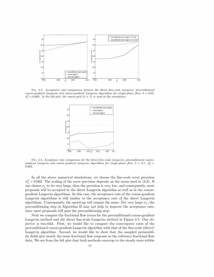
Fig. 4.2. Acceptance rate comparison between the direct fine-scale Langevin, preconditionedcoarse-gradient Langevin and coarse-gradient Langevin algorithms for single-phase flow; δ = 0.05,σ2

f= 0.003. In the left plot, the coarse-grid 11 × 11 is used in the simulation.

0.006 0.009 0.012 0.015 0.018 0.020.25

0.3

0.35

0.4

0.45

0.5

0.55

0.6

σc2

acce

pta

nce

ra

te

preconditioned coarse Langevincoarse Langevinfine scale Langevin

Fig. 4.3. Acceptance rate comparison for the direct fine-scale Langevin, preconditioned coarse-gradient Langevin and coarse-gradient Langevin algorithms for single-phase flow, δ = 0.1, σ2

f=

0.003.

In all the above numerical simulations, we choose the fine-scale error precisionσ2

f = 0.003. The scaling of the error precision depends on the norm used in (3.3). Ifone choses σf to be very large, then the precision is very low, and consequently, mostproposals will be accepted in the direct Langevin algorithm as well as in the coarse-gradient Langevin algorithms. In this case, the acceptance rate of the coarse-gradientLangevin algorithms is still similar to the acceptance rate of the direct Langevinalgorithms. Consequently, the speed-up will remain the same. For very large σf , thepreconditioning step in Algorithm II may not help to improve the acceptance rate,since most proposals will pass the preconditioning step.

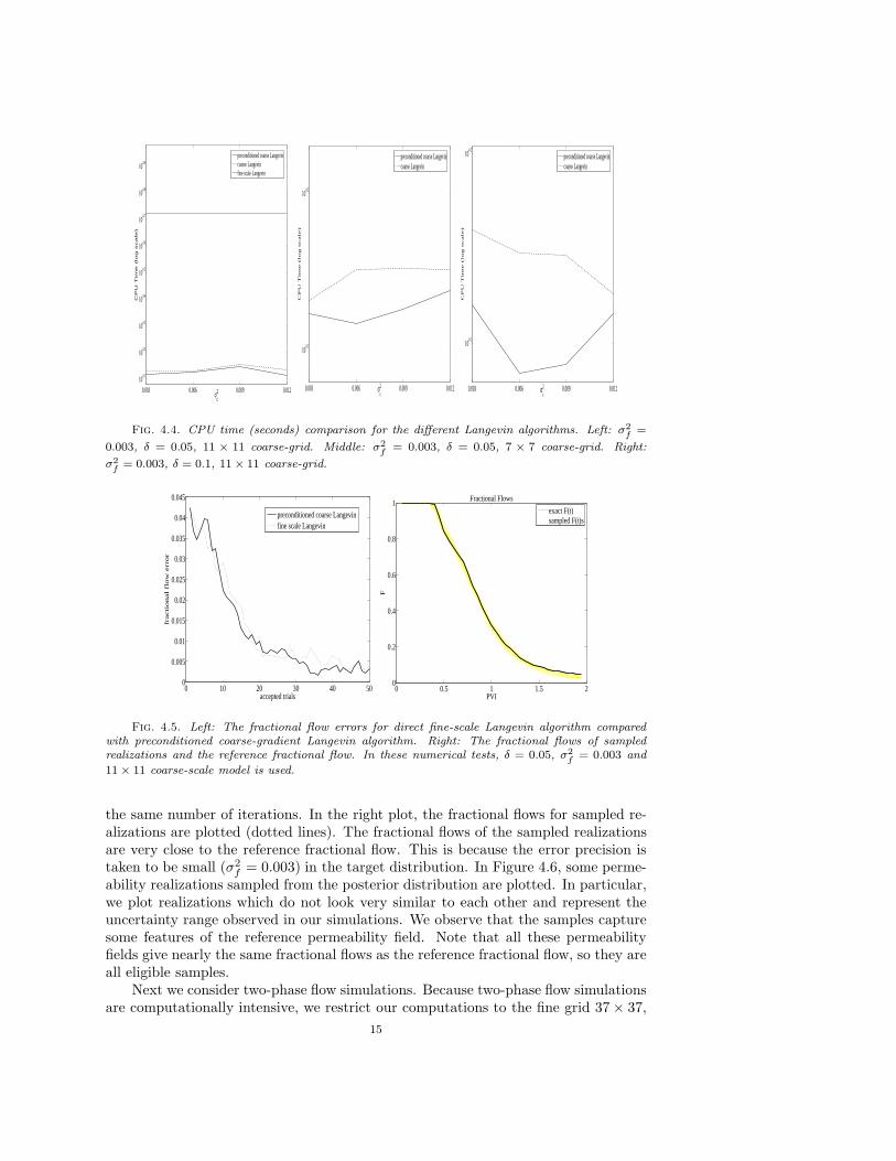
Next we compare the fractional flow errors for the preconditioned coarse-gradientLangevin method and the direct fine-scale Langevin method in Figure 4.5. Our ob-jective is two-fold. First, we would like to compare the convergence rates of thepreconditioned coarse-gradient Langevin algorithm with that of the fine-scale (direct)Langevin algorithm. Second, we would like to show that the sampled permeabil-ity fields give nearly the same fractional flow response as the reference fractional flowdata. We see from the left plot that both methods converge to the steady state within

14

0.003 0.006 0.009 0.012

104.1

104.2

104.3

104.4

104.5

104.6

104.7

104.8

104.9

σc2

CP

U T

ime

(lo

g sca

le)

preconditioned coarse Langevincoarse Langevinfine scale Langevin

0.003 0.006 0.009 0.012

104.1

104.2

σc2

CP

U T

ime

(lo

g sca

le)

preconditioned coarse Langevincoarse Langevin

0.003 0.006 0.009 0.012

104.1

104.2

σc2

CP

U T

ime

(lo

g sca

le)

preconditioned coarse Langevincoarse Langevin

Fig. 4.4. CPU time (seconds) comparison for the different Langevin algorithms. Left: σ2

f=

0.003, δ = 0.05, 11 × 11 coarse-grid. Middle: σ2

f= 0.003, δ = 0.05, 7 × 7 coarse-grid. Right:

σ2

f= 0.003, δ = 0.1, 11 × 11 coarse-grid.

0 10 20 30 40 500

0.005

0.01

0.015

0.02

0.025

0.03

0.035

0.04

0.045

accepted trials

fra

ctio

na

l flo

w e

rro

r

preconditioned coarse Langevinfine scale Langevin

0 0.5 1 1.5 20

0.2

0.4

0.6

0.8

1

PVI

F

Fractional Flows

exact F(t)sampled F(t)s

Fig. 4.5. Left: The fractional flow errors for direct fine-scale Langevin algorithm comparedwith preconditioned coarse-gradient Langevin algorithm. Right: The fractional flows of sampledrealizations and the reference fractional flow. In these numerical tests, δ = 0.05, σ2

f= 0.003 and

11 × 11 coarse-scale model is used.

the same number of iterations. In the right plot, the fractional flows for sampled re-alizations are plotted (dotted lines). The fractional flows of the sampled realizationsare very close to the reference fractional flow. This is because the error precision istaken to be small (σ2

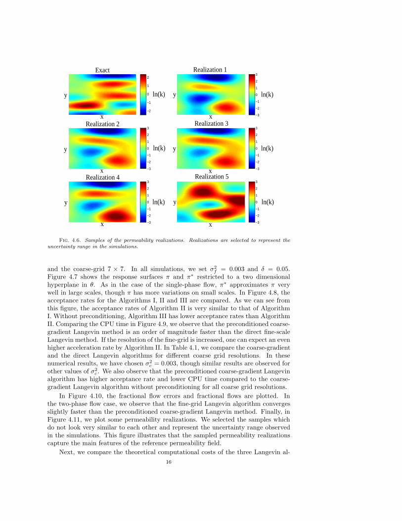
f = 0.003) in the target distribution. In Figure 4.6, some perme-ability realizations sampled from the posterior distribution are plotted. In particular,we plot realizations which do not look very similar to each other and represent theuncertainty range observed in our simulations. We observe that the samples capturesome features of the reference permeability field. Note that all these permeabilityfields give nearly the same fractional flows as the reference fractional flow, so they areall eligible samples.

Next we consider two-phase flow simulations. Because two-phase flow simulationsare computationally intensive, we restrict our computations to the fine grid 37 × 37,

15

−2

−1

0

1

2

−3

−2

−1

0

1

2

3

−3

−2

−1

0

1

2

3

−3

−2

−1

0

1

2

3

−3

−2

−1

0

1

2

3

−3

−2

−1

0

1

2

3

x

yy

x

x

y y

x

x

yy

x

Realization 4 Realization 5

Realization 3Realization 2

Realization 1Exact

ln(k)

ln(k)

ln(k)

ln(k)

ln(k)

ln(k)

Fig. 4.6. Samples of the permeability realizations. Realizations are selected to represent theuncertainty range in the simulations.

and the coarse-grid 7 × 7. In all simulations, we set σ2f = 0.003 and δ = 0.05.

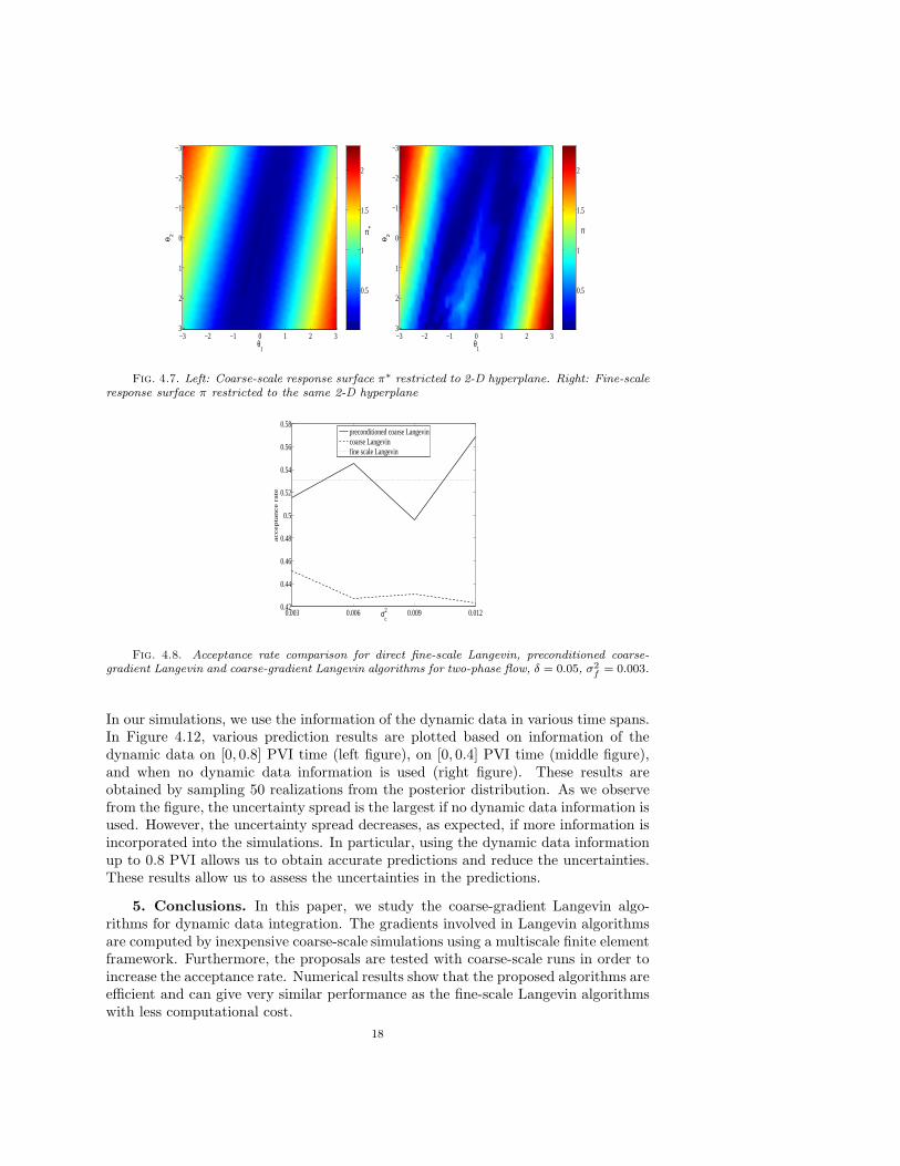
Figure 4.7 shows the response surfaces π and π∗ restricted to a two dimensionalhyperplane in θ. As in the case of the single-phase flow, π∗ approximates π verywell in large scales, though π has more variations on small scales. In Figure 4.8, theacceptance rates for the Algorithms I, II and III are compared. As we can see fromthis figure, the acceptance rates of Algorithm II is very similar to that of AlgorithmI. Without preconditioning, Algorithm III has lower acceptance rates than AlgorithmII. Comparing the CPU time in Figure 4.9, we observe that the preconditioned coarse-gradient Langevin method is an order of magnitude faster than the direct fine-scaleLangevin method. If the resolution of the fine-grid is increased, one can expect an evenhigher acceleration rate by Algorithm II. In Table 4.1, we compare the coarse-gradientand the direct Langevin algorithms for different coarse grid resolutions. In thesenumerical results, we have chosen σ2

c = 0.003, though similar results are observed forother values of σ2

c . We also observe that the preconditioned coarse-gradient Langevinalgorithm has higher acceptance rate and lower CPU time compared to the coarse-gradient Langevin algorithm without preconditioning for all coarse grid resolutions.

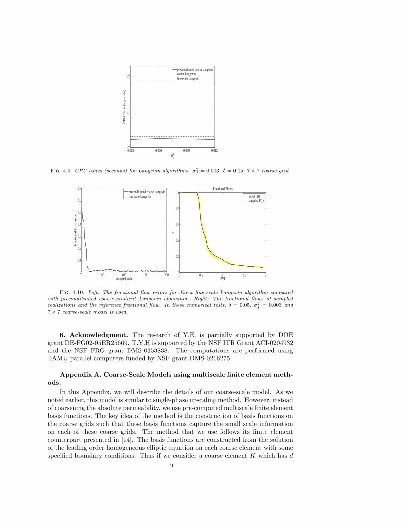
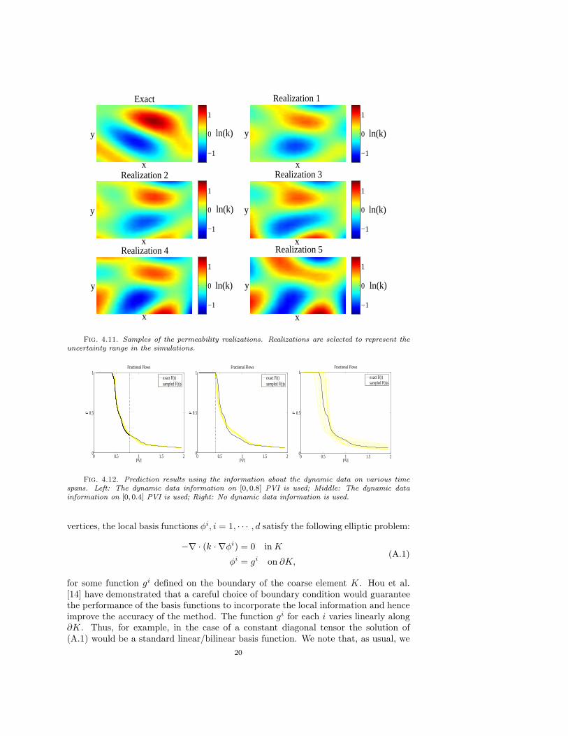
In Figure 4.10, the fractional flow errors and fractional flows are plotted. Inthe two-phase flow case, we observe that the fine-grid Langevin algorithm convergesslightly faster than the preconditioned coarse-gradient Langevin method. Finally, inFigure 4.11, we plot some permeability realizations. We selected the samples whichdo not look very similar to each other and represent the uncertainty range observedin the simulations. This figure illustrates that the sampled permeability realizationscapture the main features of the reference permeability field.

Next, we compare the theoretical computational costs of the three Langevin al-

16

Table 4.1

Comparison of Algorithm I, II and III for different coarse-grid resolutions in two-phase flowsimulations. σ2

f= σ2

c = 0.003, δ = 0.05.

coarse coarse preconditioned directcoarse grid

accept. rate CPU accept. rate CPU accept. rate CPU4x4 0.47 8527 0.55 7036 0.53 6558957x7 0.45 21859 0.52 17051 0.53 655895

10x10 0.46 70964 0.57 48653 0.53 655895

gorithms for the two-phase flow problem. Denote tf and tc as the CPU time to solvethe PDE system (2.1)-(2.3) on the fine- and coarse-grid respectively. Suppose D isthe dimension of the parameter space of the permeability field k, and N is the num-ber of proposals that are tested in all three Langevin algorithms. For each new Y ,Algorithm I needs to compute the target distribution π(Y ) and its gradient ∇π(Y ) onthe fine-grid. If the gradient is computed by the forward difference scheme, then thePDE system (2.1)-(2.3) needs to be solved on the fine-grid (D + 1) times. Therefore,the total computational cost of Algorithm I is N(D + 1)tf . For Algorithm III, thegradient of the distribution is computed on the coarse-grid. However, the acceptancetest is calculated on the fine-grid for each proposal. Thus, its computational cost isN(Dtc + tf ). In Algorithm II, the gradient of the distribution is also computed onthe coarse-grid. And each new sample is first tested by the coarse-scale distribution.If it passes the coarse-grid acceptance test, then the proposal will be further testedby the fine-scale distribution. Suppose M proposals (out of N) pass the coarse-scaletest, then the total computational cost of Algorithm II is N(D + 1)tc +Mtf . Thus,

the Algorithm II isN(D+1)tf

N(D+1)tc+Mtftimes faster than Algorithm I, and

N(Dtc+tf )N(D+1)tc+Mtf

times faster than Algorithm III. In our computations, D is of order of ten becausewe represent the permeability field by its truncated Karhunen-Loeve expansion. Ifthe fine-scale model is scaled up 6 times in each direction, as we did in the numer-ical experiment, then the coarse-scale model is approximately 36 times faster thanthe fine-scale model. Indeed, at each time step solving the pressure equation on thecoarse grid is approximately 36 times faster than on the fine grid. The same is truefor the saturation equation since it is also solved on the coarse grid and with largertime steps. Moreover, in the preconditioned coarse-gradient Langevin algorithm, onlya portion of the N proposals can pass the coarse-scale test, where N is usually twotimes larger than M . Using these estimates, we expect that the CPU time of thepreconditioned coarse-gradient Langevin algorithms should be an order of magnitudelower than that of the fine-scale Langevin algorithm. We indeed observed a similarspeedup in our computations, as demonstrated by Figure 4.9.

Note that one can use simple random walk samplers, instead of the Langevinalgorithm, in Algorithm I. We have observed in our numerical experiments that theacceptance rate of the random walk sampler is several times smaller than that ofLangevin algorithms. This is not surprising because Langevin algorithms use thegradient information of the target distribution and are problem adapted. One canalso use single-phase flow upscaling (as in [5]) in the preconditioning step as it isdone in [9]. In general, we have found the multiscale methods to be more accurate forcoarse-scale simulations and they can be further used for efficient and robust fine-scalesimulations.

Finally, we present the results demonstrating the uncertainties in the predictions.

17

θ1

θ2

−3 −2 −1 0 1 2 3

−3

−2

−1

0

1

2

3

0.5

1

1.5

2

π*

θ1

θ2

−3 −2 −1 0 1 2 3

−3

−2

−1

0

1

2

3

0.5

1

1.5

2

π

Fig. 4.7. Left: Coarse-scale response surface π∗ restricted to 2-D hyperplane. Right: Fine-scaleresponse surface π restricted to the same 2-D hyperplane

0.003 0.006 0.009 0.0120.42

0.44

0.46

0.48

0.5

0.52

0.54

0.56

0.58

σc2

acce

pta

nce

ra

te

preconditioned coarse Langevincoarse Langevinfine scale Langevin

Fig. 4.8. Acceptance rate comparison for direct fine-scale Langevin, preconditioned coarse-gradient Langevin and coarse-gradient Langevin algorithms for two-phase flow, δ = 0.05, σ2

f= 0.003.

In our simulations, we use the information of the dynamic data in various time spans.In Figure 4.12, various prediction results are plotted based on information of thedynamic data on [0, 0.8] PVI time (left figure), on [0, 0.4] PVI time (middle figure),and when no dynamic data information is used (right figure). These results areobtained by sampling 50 realizations from the posterior distribution. As we observefrom the figure, the uncertainty spread is the largest if no dynamic data information isused. However, the uncertainty spread decreases, as expected, if more information isincorporated into the simulations. In particular, using the dynamic data informationup to 0.8 PVI allows us to obtain accurate predictions and reduce the uncertainties.These results allow us to assess the uncertainties in the predictions.

5. Conclusions. In this paper, we study the coarse-gradient Langevin algo-rithms for dynamic data integration. The gradients involved in Langevin algorithmsare computed by inexpensive coarse-scale simulations using a multiscale finite elementframework. Furthermore, the proposals are tested with coarse-scale runs in order toincrease the acceptance rate. Numerical results show that the proposed algorithms areefficient and can give very similar performance as the fine-scale Langevin algorithmswith less computational cost.

18

0.003 0.006 0.009 0.01210

4

105

106

σc2

CP

U T

ime

(lo

g s

ca

le)

preconditioned coarse Langevincoarse Langevinfine scale Langevin

Fig. 4.9. CPU times (seconds) for Langevin algorithms. σ2

f= 0.003, δ = 0.05, 7 × 7 coarse-grid.

0 50 100 150 2000

0.1

0.2

0.3

0.4

0.5

0.6

0.7

accepted trials

fra

ctio

na

l flo

w e

rro

r

preconditioned coarse Langevinfine scale Langevin

0 0.5 1 1.5 20

0.2

0.4

0.6

0.8

1

PVI

F

Fractional Flows

exact F(t)sampled F(t)s

Fig. 4.10. Left: The fractional flow errors for direct fine-scale Langevin algorithm comparedwith preconditioned coarse-gradient Langevin algorithm. Right: The fractional flows of sampledrealizations and the reference fractional flow. In these numerical tests, δ = 0.05, σ2

f= 0.003 and

7 × 7 coarse-scale model is used.

6. Acknowledgment. The research of Y.E. is partially supported by DOEgrant DE-FG02-05ER25669. T.Y.H is supported by the NSF ITR Grant ACI-0204932and the NSF FRG grant DMS-0353838. The computations are performed usingTAMU parallel computers funded by NSF grant DMS-0216275.

Appendix A. Coarse-Scale Models using multiscale finite element meth-ods.

In this Appendix, we will describe the details of our coarse-scale model. As wenoted earlier, this model is similar to single-phase upscaling method. However, insteadof coarsening the absolute permeability, we use pre-computed multiscale finite elementbasis functions. The key idea of the method is the construction of basis functions onthe coarse grids such that these basis functions capture the small scale informationon each of these coarse grids. The method that we use follows its finite elementcounterpart presented in [14]. The basis functions are constructed from the solutionof the leading order homogeneous elliptic equation on each coarse element with somespecified boundary conditions. Thus if we consider a coarse element K which has d

19

−1

0

1

−1

0

1

−1

0

1

−1

0

1

−1

0

1

−1

0

1

ln(k)

ln(k)

ln(k)

ln(k)

ln(k)

ln(k)

Exact Realization 1

Realization 2 Realization 3

Realization 5Realization 4

x

y y

x

x

yy

x

x

y y

x

Fig. 4.11. Samples of the permeability realizations. Realizations are selected to represent theuncertainty range in the simulations.

0 0.5 1 1.5 20

0.5

1

PVI

F

Fractional Flows

exact F(t)sampled F(t)s

0 0.5 1 1.5 20

0.5

1

PVI

F

Fractional Flows

exact F(t)sampled F(t)s

0 0.5 1 1.5 20

0.5

1

PVI

F

Fractional Flows

exact F(t)sampled F(t)s

Fig. 4.12. Prediction results using the information about the dynamic data on various timespans. Left: The dynamic data information on [0, 0.8] PVI is used; Middle: The dynamic datainformation on [0, 0.4] PVI is used; Right: No dynamic data information is used.

vertices, the local basis functions φi, i = 1, · · · , d satisfy the following elliptic problem:

−∇ · (k · ∇φi) = 0 inK

φi = gi on ∂K,(A.1)

for some function gi defined on the boundary of the coarse element K. Hou et al.[14] have demonstrated that a careful choice of boundary condition would guaranteethe performance of the basis functions to incorporate the local information and henceimprove the accuracy of the method. The function gi for each i varies linearly along∂K. Thus, for example, in the case of a constant diagonal tensor the solution of(A.1) would be a standard linear/bilinear basis function. We note that, as usual, we

20

require φi(ξj) = δij . Finally, a nodal basis function associated with the vertex ξ in thedomain Ω is constructed from the combination of the local basis functions that sharethis ξ and zero elsewhere. These nodal basis functions are denoted by ψξξ∈Z0

h.

Having described the basis functions, we denote by V h the space of our approx-imate pressure solution which is spanned by the basis functions ψξξ∈Z0

h. Now we

may formulate the finite dimensional problem corresponding to the finite volume ele-ment formulation of (2.2). A statement of mass conservation on a control volume Vξ

is formed from (2.2), where now the approximate solution is written as a linear combi-nation of the basis functions. Assembly of this conservation statement for all controlvolumes would give the corresponding linear system of equations that can be solvedaccordingly. The resulting linear system has incorporated the fine-scale informationthrough the involvement of the nodal basis functions on the approximate solution. Tobe specific, the problem now is to seek ph ∈ V h with ph =

∑

ξ∈Z0

hpξψξ such that

∫

∂Vξ

λ(S)k · ∇ph · ~n dl =

∫

Vξ

f dA, (A.2)

for every control volume Vξ ⊂ Ω. Here ~n defines the unit normal vector on theboundary of the control volume, ∂Vξ, and S is the fine scale saturation field at thispoint. We note that, concerning the basis functions, a vertex-centered finite volumedifference is used to solve (A.1), and a harmonic average is employed to approximatethe permeability k at the edges of fine control volumes.

Furthermore, the pressure solution may be used to compute the total velocity fieldat the coarse-scale level, denoted by v = (vx, vz) via (2.6). In general, the followingequations are used to compute the velocities in horizontal and vertical directions,respectively:

vx = − 1

hz

∑

ξ∈Z0

h

pξ

(∫

E

λ(S)kx

∂ψξ

∂xdz

)

, (A.3)

vz = − 1

hx

∑

ξ∈Z0

h

pξ

(∫

E

λ(S)kz

∂ψξ

∂zdx

)

, (A.4)

where E is the edge of Vξ. Furthermore, for the control volumes Vξ adjacent tothe Dirichlet boundary (which are half control volumes), we can derive the velocityapproximation using the conservation statement derived from (2.2) on Vξ. One of theterms involved is the integration along part of the Dirichlet boundary, while the restof the three terms are known from the adjacent internal control volumes calculations.The analysis of the two-scale finite volume method can be found in [11].

As for the upscaling of the saturation equation, we only use the coarse scalevelocity to update the saturation field on the coarse-grid, i.e.,

∂S

∂t+ v · ∇f(S) = 0, (A.5)

where S denotes the saturation on the coarse-grid. In this case the upscaling of thesaturation equation does not take into account subgrid effects. This kind of upscalingtechniques in conjunction with the upscaling of absolute permeability are commonlyused in applications (see e.g. [6, 7, 8]). The difference of our approach is that thecoupling of the small scales is performed through the finite volume element formulationof the pressure equation.

21

REFERENCES

[1] J. W. Barker and S. Thibeau, A critical review of the use of pseudo-relative permeabilitiesfor upscaling, SPE Res. Eng., 12 (1997), pp. 138–143.

[2] A. Christen and C. Fox, MCMC using an approximation. Technical report, Department ofMathematics, The University of Auckland, New Zealand.

[3] M. Christie, Upscaling for reservoir simulation, J. Pet. Tech., (1996), pp. 1004–1010.[4] C. V. Deutsch and A. G. Journel, GSLIB: Geostatistical software library and user’s guide,

2nd edition, Oxford University Press, New York, 1998.[5] L. J. Durlofsky, Numerical calculation of equivalent grid block permeability tensors for het-

erogeneous porous media, Water Resour. Res., 27 (1991), pp. 699–708.[6] , Coarse scale models of two phase flow in heterogeneous reservoirs: Volume averaged

equations and their relationship to the existing upscaling techniques, Computational Geo-sciences, 2 (1998), pp. 73–92.

[7] L. J. Durlofsky, R. A. Behrens, R. C. Jones, and A. Bernath, Scale up of heterogeneousthree dimensional reservoir descriptions, SPE paper 30709, (1996).

[8] L. J. Durlofsky, R. C. Jones, and W. J. Milliken, A nonuniform coarsening approachfor the scale up of displacement processes in heterogeneous media, Advances in WaterResources, 20 (1997), pp. 335–347.

[9] Y. Efendiev, A. Datta-Gupta, V. Ginting, X. Ma, and B. Mallick, An efficient two-stageMarkov chain Monte Carlo method for dynamic data integration. Accepted for publication.Water Resources Research.

[10] Y. Efendiev, T. Hou and W. Luo, Preconditioning Markov chain Monte Carlo simulationsusing coarse-scale models. Accepted for publication. SIAM Sci. Comp.

[11] V. Ginting, Analysis of two-scale finite volume element method for elliptic problem, Journalof Numerical Mathematics, 12(2) (2004), pp. 119–142.

[12] J. Glimm and D. H. Sharp, Prediction and the quantification of uncertainty, Phys. D, 133(1999), pp. 152–170. Predictability: quantifying uncertainty in models of complex phe-nomena (Los Alamos, NM, 1998).

[13] U. Grenander and M.I. Miller, Representations of knowledge in complex systems (withdiscussion), J. R. Statist. Soc. B, 56 (1994), 549-603.

[14] T. Y. Hou and X. H. Wu, A multiscale finite element method for elliptic problems in compositematerials and porous media, Journal of Computational Physics, 134 (1997), pp. 169–189.

[15] L. Hu, Gradual deformation and iterative calibration of Gaussian-related stochastic models,Mathematical Geology, 32(1) (2000), pp. 87–108.

[16] P. Kitanidis, Quasi-linear geostatistical theory for inversing, Water Resour. Res., 31 (1995),pp. 2411–2419.

[17] J. S. Liu, Monte Carlo Strategies in Scientific Computing, Springer, New-York, 2001.[18] O. Lodoen, H. Omre, L. Durlofsky, and Y. Chen, Assessment of uncertainty in reser-

voir production forecasts using upscaled models. Presented at the Seventh InternationalGeostatistics Congress, Banff, Canada, Sept. 26-Oct. 1 2004.

[19] M. Loeve, Probability Theory, 4th ed., Springer, Berlin, 1977.[20] S. P. Meyn, R. L. Tweedie, Markov Chains and Stochastic Stability, Springer-Verlag, London,

1996.[21] D. Oliver, L. Cunha, and A. Reynolds, Markov chain Monte Carlo methods for conditioning

a permeability field to pressure data, Mathematical Geology, 29 (1997).[22] D. Oliver, N. He, and A. Reynolds, Conditioning permeability fields to pressure data. 5th

European conference on the mathematics of oil recovery, Leoben, Austria, 3-6 September,1996.

[23] C. Robert and G. Casella, Monte Carlo Statistical Methods, Springer-Verlag, New-York,1999.

[24] E. Wong, Stochastic Processes in Information and Dynamical Systems, MCGraw-Hill, 1971.

22