ChemicalScience

EDGE ARTICLE

Ope

n A

cces

s A

rtic

le. P

ublis

hed

on 1

8 M

ay 2

021.

Dow

nloa

ded

on 1

1/18

/202

1 5:

14:1

9 A

M.

Thi

s ar

ticle

is li

cens

ed u

nder

a C

reat

ive

Com

mon

s A

ttrib

utio

n-N

onC

omm

erci

al 3

.0 U

npor

ted

Lic

ence

.

View Article OnlineView Journal | View Issue

Coacervate form

aGroningen Biomolecular Sciences and Biot

for Advanced Materials, University of

Netherlands. E-mail: s.j.marrink@rug.nlbMolecular Microbiology and Structural Bioc

Lyon, Lyon, France

† Electronic supplementary informa10.1039/d1sc00374g

Cite this: Chem. Sci., 2021, 12, 8521

All publication charges for this articlehave been paid for by the Royal Societyof Chemistry

Received 20th January 2021Accepted 17th May 2021

DOI: 10.1039/d1sc00374g

rsc.li/chemical-science

© 2021 The Author(s). Published by

ation studied by explicit solventcoarse-grain molecular dynamics with the Martinimodel†

Maria Tsanai, a Pim W. J. M. Frederix, a Carsten F. E. Schroer,a

Paulo C. T. Souza ab and Siewert J. Marrink *a

Complex coacervates are liquid–liquid phase separated systems, typically containing oppositely charged

polyelectrolytes. They are widely studied for their functional properties as well as their potential

involvement in cellular compartmentalization as biomolecular condensates. Diffusion and partitioning of

solutes into a coacervate phase are important to address because their highly dynamic nature is one of

their most important functional characteristics in real-world systems, but are difficult to study

experimentally or even theoretically without an explicit representation of every molecule in the system.

Here, we present an explicit-solvent, molecular dynamics coarse-grain model of complex coacervates,

based on the Martini 3.0 force field. We demonstrate the accuracy of the model by reproducing the salt

dependent coacervation of poly-lysine and poly-glutamate systems, and show the potential of the

model by simulating the partitioning of ions and small nucleotides between the condensate and

surrounding solvent phase. Our model paves the way for simulating coacervates and biomolecular

condensates in a wide range of conditions, with near-atomic resolution.

1 Introduction

Solutions of oppositely charged polyions may show liquid–liquid phase coexistence. Depending on the state conditions(e.g. salt concentration, polymer concentration, pH andtemperature), electrostatically driven complex formation canlead to phase separation between macromolecule-rich andmacromolecule-decient fractions. Already since the early 20thcentury, this process is known as coacervation, and it is regu-larly found in naturally occurring charged colloids, such asserum albumin and gum arabic.1 Since then, many combina-tions of natural or synthetic macro-ions have been shown toform complex coacervates and they have started to nd appli-cations in the encapsulation or extraction of small activecompounds for biomedicine.2,3 Additionally, the liquid–liquidphase separation leads to formation of liquid droplets thatcould serve as membraneless compartments in aqueous solu-tion, a potentially important intermediate step in the earlyformation of living cells.4 Moreover, evidence is mounting thatpresent-day cells feature multiple cellular compartments that

echnology Institute and Zernike Institute

Groningen, 9747AG Groningen, The

hemistry, UMR 5086 CNRS, University of

tion (ESI) available. See DOI:

the Royal Society of Chemistry

are characterized by liquid properties (biomolecular conden-sates), including high turnover of components and easydeformation.5–14

One of the current challenges for the eld is to study thedynamics of individual molecules (not only polyelectrolytes, butalso solvent, ions and small organic compounds) inside thecoacervate phase. Some experimental methods such as Over-hauser dynamic nuclear polarization (ODNP) measurementscan probe the local dynamics of polymers or water when spinlabels are added,15 but explicit molecular simulation techniquessuch as Molecular Dynamics (MD) are arguably more versatilein addressing this challenge. All-atom MD simulations have sofar mainly been restricted to simulating pairs of electrolytemolecules, as simulating systems with multiple polymer chainsrepresentative of a coacervate becomes computationallyexpensive and the sampling of the relevant conformationsbecomes problematic.16–18 A recent exception is the study byMintis and Mavrantzas,19 who used a free energy basedapproach with an explicit solvent all-atom model to study thephase diagram of short acrylic polymer fragments. Neglectingthe solvent degrees of freedom remedies this problem to someextent,20,21 but the importance of explicit water in simulatingpolyelectrolyte complex formation was demonstrated ina number of cases.22–25 Given the limitations of all-atommodels,the use of coarse-grain (CG) models is gaining popularity in thiseld.26 In coarse-graining, groups of atoms are represented byeffective interaction sites, drastically reducing the number ofparticles.27 CG MD allows to describe the diffusive and

Chem. Sci., 2021, 12, 8521–8530 | 8521

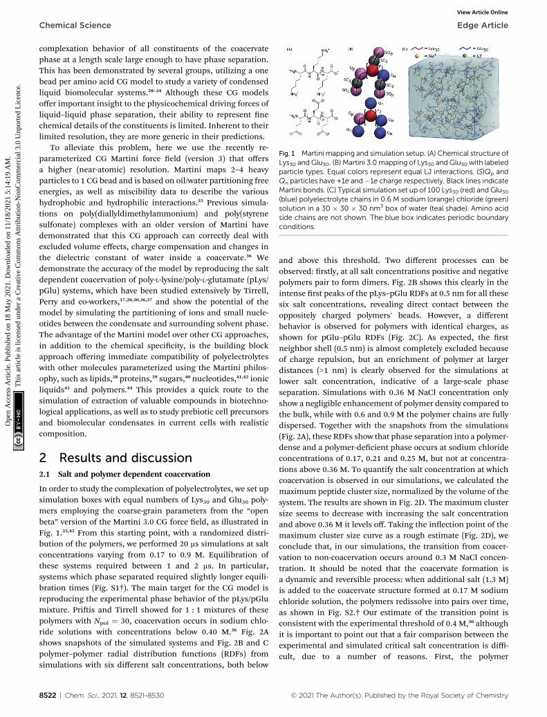
Fig. 1 Martini mapping and simulation setup. (A) Chemical structure ofLys30 and Glu30. (B) Martini 3.0mapping of Lys30 and Glu30 with labeledparticle types. Equal colors represent equal LJ interactions. (S)Qp andQn particles have +1e and�1e charge respectively. Black lines indicateMartini bonds. (C) Typical simulation set up of 100 Lys30 (red) and Glu30(blue) polyelectrolyte chains in 0.6 M sodium (orange) chloride (green)solution in a 30 � 30 � 30 nm3 box of water (teal shade). Amino acidside chains are not shown. The blue box indicates periodic boundaryconditions.

Chemical Science Edge Article

Ope

n A

cces

s A

rtic

le. P

ublis

hed

on 1

8 M

ay 2

021.

Dow

nloa

ded

on 1

1/18

/202

1 5:

14:1

9 A

M.

Thi

s ar

ticle

is li

cens

ed u

nder

a C

reat

ive

Com

mon

s A

ttrib

utio

n-N

onC

omm

erci

al 3

.0 U

npor

ted

Lic

ence

.View Article Online

complexation behavior of all constituents of the coacervatephase at a length scale large enough to have phase separation.This has been demonstrated by several groups, utilizing a onebead per amino acid CG model to study a variety of condensedliquid biomolecular systems.28–34 Although these CG modelsoffer important insight to the physicochemical driving forces ofliquid–liquid phase separation, their ability to represent nechemical details of the constituents is limited. Inherent to theirlimited resolution, they are more generic in their predictions.

To alleviate this problem, here we use the recently re-parameterized CG Martini force eld (version 3) that offersa higher (near-atomic) resolution. Martini maps 2–4 heavyparticles to 1 CG bead and is based on oil/water partitioning freeenergies, as well as miscibility data to describe the varioushydrophobic and hydrophilic interactions.35 Previous simula-tions on poly(diallyldimethylammonium) and poly(styrenesulfonate) complexes with an older version of Martini havedemonstrated that this CG approach can correctly deal withexcluded volume effects, charge compensation and changes inthe dielectric constant of water inside a coacervate.36 Wedemonstrate the accuracy of the model by reproducing the saltdependent coacervation of poly-L-lysine/poly-L-glutamate (pLys/pGlu) systems, which have been studied extensively by Tirrell,Perry and co-workers,17,20,30,36,37 and show the potential of themodel by simulating the partitioning of ions and small nucle-otides between the condensate and surrounding solvent phase.The advantage of the Martini model over other CG approaches,in addition to the chemical specicity, is the building blockapproach offering immediate compatibility of polyelectrolyteswith other molecules parameterized using the Martini philos-ophy, such as lipids,38 proteins,39 sugars,40 nucleotides,41,42 ionicliquids43 and polymers.44 This provides a quick route to thesimulation of extraction of valuable compounds in biotechno-logical applications, as well as to study prebiotic cell precursorsand biomolecular condensates in current cells with realisticcomposition.

2 Results and discussion2.1 Salt and polymer dependent coacervation

In order to study the complexation of polyelectrolytes, we set upsimulation boxes with equal numbers of Lys30 and Glu30 poly-mers employing the coarse-grain parameters from the “openbeta” version of the Martini 3.0 CG force eld, as illustrated inFig. 1.35,45 From this starting point, with a randomized distri-bution of the polymers, we performed 20 ms simulations at saltconcentrations varying from 0.17 to 0.9 M. Equilibration ofthese systems required between 1 and 2 ms. In particular,systems which phase separated required slightly longer equili-bration times (Fig. S1†). The main target for the CG model isreproducing the experimental phase behavior of the pLys/pGlumixture. Priis and Tirrell showed for 1 : 1 mixtures of thesepolymers with Npol ¼ 30, coacervation occurs in sodium chlo-ride solutions with concentrations below 0.40 M.36 Fig. 2Ashows snapshots of the simulated systems and Fig. 2B and Cpolymer–polymer radial distribution functions (RDFs) fromsimulations with six different salt concentrations, both below

8522 | Chem. Sci., 2021, 12, 8521–8530

and above this threshold. Two different processes can beobserved: rstly, at all salt concentrations positive and negativepolymers pair to form dimers. Fig. 2B shows this clearly in theintense rst peaks of the pLys–pGlu RDFs at 0.5 nm for all thesesix salt concentrations, revealing direct contact between theoppositely charged polymers' beads. However, a differentbehavior is observed for polymers with identical charges, asshown for pGlu–pGlu RDFs (Fig. 2C). As expected, the rstneighbor shell (0.5 nm) is almost completely excluded becauseof charge repulsion, but an enrichment of polymer at largerdistances (>1 nm) is clearly observed for the simulations atlower salt concentration, indicative of a large-scale phaseseparation. Simulations with 0.36 M NaCl concentration onlyshow a negligible enhancement of polymer density compared tothe bulk, while with 0.6 and 0.9 M the polymer chains are fullydispersed. Together with the snapshots from the simulations(Fig. 2A), these RDFs show that phase separation into a polymer-dense and a polymer-decient phase occurs at sodium chlorideconcentrations of 0.17, 0.21 and 0.25 M, but not at concentra-tions above 0.36 M. To quantify the salt concentration at whichcoacervation is observed in our simulations, we calculated themaximum peptide cluster size, normalized by the volume of thesystem. The results are shown in Fig. 2D. The maximum clustersize seems to decrease with increasing the salt concentrationand above 0.36 M it levels off. Taking the inection point of themaximum cluster size curve as a rough estimate (Fig. 2D), weconclude that, in our simulations, the transition from coacer-vation to non-coacervation occurs around 0.3 M NaCl concen-tration. It should be noted that the coacervate formation isa dynamic and reversible process: when additional salt (1.3 M)is added to the coacervate structure formed at 0.17 M sodiumchloride solution, the polymers redissolve into pairs over time,as shown in Fig. S2.† Our estimate of the transition point isconsistent with the experimental threshold of 0.4 M,30 althoughit is important to point out that a fair comparison between theexperimental and simulated critical salt concentration is diffi-cult, due to a number of reasons. First, the polymer

© 2021 The Author(s). Published by the Royal Society of Chemistry

Fig. 2 Salt-dependent coacervation. (A) Snapshots of the final state of 100 Lys30 and 100 Glu30 polymers after 20 ms of CG MD simulations atdifferent salt concentrations. Color code is the same as in Fig. 1, water not shown. (B) pLys–pGlu RDFs at different salt concentrations. (C) pGlu–pGlu RDFs at different salt concentrations. (D) Maximum peptide cluster size at different salt concentrations normalized by the volume of eachsystem (for a cut-off of 0.6 nm, which is the largest distance to be considered as a cluster).

Edge Article Chemical Science

Ope

n A

cces

s A

rtic

le. P

ublis

hed

on 1

8 M

ay 2

021.

Dow

nloa

ded

on 1

1/18

/202

1 5:

14:1

9 A

M.

Thi

s ar

ticle

is li

cens

ed u

nder

a C

reat

ive

Com

mon

s A

ttrib

utio

n-N

onC

omm

erci

al 3

.0 U

npor

ted

Lic

ence

.View Article Online

concentrations used in the simulations are much higher thanthose used in the experiments, to keep the simulations tractable(otherwise mostly water–water interactions would be simu-lated). Potentially, the miscibility transition depends on thepolymer concentration. Unfortunately, the extent of this effect isnot known for the system under investigation, but experimentaldata for similar systems (pHis/pGlu complex coacervate) pointto a limited effect.30 Similar to the polymer length, an increaseof 2 to 10 times the polymer concentration seems to promotea shi to modestly higher concentrations of salt, in the range of0.2 to 0.5 M. Second, our simulation boxes are periodic, andlimited in size, and therefore nite size effects are likely to play

© 2021 The Author(s). Published by the Royal Society of Chemistry

a role. To obtain a more accurate estimate of precise phaseboundaries, Gibbs-ensemble simulations are a suitable choice,as demonstrated by several groups in the context of LLPS.19,31,34

However, such simulations are computationally ratherdemanding as they rely on Monte-Carlo moves, which is nottrivial for polymer-based systems with near-atomic detail.Third, the exact transition point is rather sensitive to details ofthe force eld. We noticed a shi of the transition point tohigher salt concentration when using the nal Martini 3.0version instead of the beta release (Fig. S3†), which certainlyimproves the match with the experimental transition point.Keeping these limitations in mind, we conclude that our model

Chem. Sci., 2021, 12, 8521–8530 | 8523

Chemical Science Edge Article

Ope

n A

cces

s A

rtic

le. P

ublis

hed

on 1

8 M

ay 2

021.

Dow

nloa

ded

on 1

1/18

/202

1 5:

14:1

9 A

M.

Thi

s ar

ticle

is li

cens

ed u

nder

a C

reat

ive

Com

mon

s A

ttrib

utio

n-N

onC

omm

erci

al 3

.0 U

npor

ted

Lic

ence

.View Article Online

captures the experimentally observed salt-dependency of thecoacervation, at least at a semi-quantitative level.

To exemplify the effect of polymer concentration to someextent, we performed additional simulations at varyingpolymer/water weight ratio. We found that polymer concentra-tion did not inuence the coacervation as strongly as saltconcentration. Simulations with 10, 50, 100 and 150 polymerchains of each charge (0.5–8% w/w) with 0.17 M salt concen-tration show aggregation in each case (except for the lowestconcentration), with the polymer-rich phase taking upa considerable part of the simulation box at the highest polymerconcentration (Fig. S4†). Priis et al. show the formation ofcoacervate droplets from 0.1 wt% total polymer concentration.With further increase of the total polymer concentration morecomplex is formed due to the increase of the available chargedsites.36

Fig. 3 Distribution of ions across coexisting phases. (A) Normalizeddensity profiles calculated for polypeptides (red), water (light blue) andNa+ and Cl� ions (green). The coacervate phase is slightly depleted ofions and water. (B) Snapshot of the extended system at 0.17 M saltconcentration. (C) Hydration of the peptides inside the coacervatephase. In this zoomed viewwater molecules are represented with cyantransparent surface. On the right side, water beads within the coac-ervate phase are shown in cyan spheres. The rest of the coacervatephase has been removed to provide a clearer view.

2.2 Ion partitioning and hydration of the coacervate phase

An important driving force behind coacervation is the release ofsmall counter-ions that were initially “bound” to the polymers,although also polymer–polymer contacts play a role.46–48 TheMD simulations show a rapid decrease of polymer-ion contactsaer complexation compared to the beginning of the simula-tion where polymers are randomly dispersed, as seen inpolymer-ion RDFs (Fig. S5†). While the classical analyticaltheories predict that ions will preferentially stay in the coacer-vate phase when they are released from the polymers bycomplexation, recent discoveries suggest that ions dissolve intothe polymer-dilute phase, ascribing the difference to the prob-lems of Voorn–Overbeek-based theories at high polymer andsalt concentrations, and the lack of molecular details such asexcluded volume effects and the reduced entropy gain from ionsrelease at the polymer ends.47,49,50 We have direct access to therelative concentrations of all components between the twophases. A straightforward way to analyze this data is bycomputing the densities of the components across the system.To have a clear denition of the two phases, we performedadditional simulations of an extended system (see Methods fordetails). The resulting densities for the peptides can beobserved in the density proles for the peptides, ions and waterin the system of 0.17 M salt concentration, as seen in Fig. 3.Although the coacervate phase contains a large amount of watermolecules and ions, the ion concentration in the bulk phase ishigher than in the coacervate phase which is in line withexperimental as well as with results from all-atom simula-tions.19,30 Note that the density of water inside the coacervatephase is reduced even more compared to the density of ions(Fig. 3A). Therefore, the effective ion concentration (amount ofions per water) is actually increased in this region.

Another interesting observation is the broad width of theinterface between the condensate and the aqueous solution.The maximum bulk density of the condensate is only reached atthe very center of the phase, implying an interfacial width ofaround 20 nm. This suggests a low surface tension (g) betweenthe two phases. To quantify this, we computed the surfacetension for the extended system based on the pressure

8524 | Chem. Sci., 2021, 12, 8521–8530

differences between the lateral and perpendicular directions(see Methods). Although this is a slowly converging property, weobserve convergence to a value of �3 bar nm on a time scale of10 ms (Fig. S6†). This low surface tension is in reasonableagreement with experimental ndings performed for the samesystem with 0.16 M NaCl concentration which report a value ofg ¼ 7 bar nm.51

2.3 Water and peptide diffusion

Experimental studies employing ODNP52 have reported a slow-ing down of water from D ¼ 2.3 � 10�9 m2 s�1 in bulk water to�1.3 � 10�9 m2 s�1 at the surface of uncomplexed polymer andto D � 0.25 � 10�9 m2 s�1 inside a coacervate phase of poly-aspartate with poly(vinylimidazole).52 Although it is difficult todirectly compare diffusion coefficients in CGMD simulations toexperiments, due to the smoothness of the CG potential energylandscape,38,53 it would be interesting to see whether a similarqualitative slowdown can be observed in our simulations as

© 2021 The Author(s). Published by the Royal Society of Chemistry

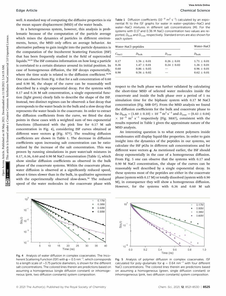
Table 1 Diffusion coefficients (10�9 m2 s�1) calculated by an expo-nential fit to the ISF graphs for water in water–peptides–NaCl andwater–NaCl mixtures in different salt concentrations (M). For thesystems with 0.17 and 0.36 M NaCl concentration two values are re-ported,Dbulk andDcoac respectively. Standard errors are also shown foreach system

Water–NaCl–peptides Water–NaCl

CNaCl Dbulk Dcoac Dbulk

0.17 1.56 � 0.01 0.26 � 0.01 1.71 � 0.010.36 1.47 � 0.01 0.24 � 0.02 1.36 � 0.010.60 0.86 � 0.05 — 0.96 � 0.010.90 0.56 � 0.02 — 0.62 � 0.01

Edge Article Chemical Science

Ope

n A

cces

s A

rtic

le. P

ublis

hed

on 1

8 M

ay 2

021.

Dow

nloa

ded

on 1

1/18

/202

1 5:

14:1

9 A

M.

Thi

s ar

ticle

is li

cens

ed u

nder

a C

reat

ive

Com

mon

s A

ttrib

utio

n-N

onC

omm

erci

al 3

.0 U

npor

ted

Lic

ence

.View Article Online

well. A standard way of computing the diffusive properties is viathe mean square displacement (MSD) of the water beads.

In a heterogeneous system, however, this analysis is prob-lematic because of the computation of the particle averagewhich mixes the dynamics of particles in different environ-ments, hence, the MSD only offers an average behavior. Analternative pathway to gain insight into the particle dynamics isthe computation of the Incoherent Scattering Function (ISF)that has been frequently studied in the eld of supercooledliquids.54,55 The ISF contains information on how long a particleis correlated to a certain distance around its initial position. Incase of homogeneous diffusion, the ISF decays exponentially,where the time scale is related to the diffusion coefficient.54,56

One can observe from Fig. 4 that for a salt concentration of 0.60and 0.90 M, the shape of the curve can be reasonably welldescribed by a single exponential decay. For the systems with0.17 and 0.36 M salt concentration, a single exponential func-tion (light green) clearly fails to describe the shape of the ISF.Instead, two distinct regimes can be observed: a fast decay thatcorresponds to the water beads in the bulk and a slow decay thatrepresents the water beads in the coacervate. In order to extractthe diffusion coefficients from the curve, we tted the datapoints in these cases with a weighted sum of two exponentialfunctions (illustrated with the pink line for 0.17 M saltconcentration in Fig. 4), considering ISF curves obtained atdifferent wave vectors q (Fig. S7†). The resulting diffusioncoefficients are shown in Table 1. The decrease in diffusioncoefficients upon increasing salt concentration can be ratio-nalized by the increase of the salt concentration. This wasproven by running simulations in pure water/salt mixtures in0.17, 0.36, 0.60 and 0.90 M NaCl concentration (Table 1), whichshow similar diffusion coefficients as observed in the bulkphase of the coacervate systems. Within the coacervate phase,water diffusion is observed at a signicantly reduced speed,about 6 times slower than in the bulk, in qualitative agreementwith the experimentally observed slow-down.52 The reducedspeed of the water molecules in the coacervate phase with

Fig. 4 Analysis of water diffusion in complex coacervates. The Inco-herent Scattering Function (ISF) with q¼ 0.5 nm�1, which correspondsto a length scale of �3.75 particle diameters, is shown for the differentsalt concentrations. The colored lines therein are predictions based onassuming a homogeneous (single diffusion constant) or inhomoge-neous (pink, two diffusion constants) system composition.

© 2021 The Author(s). Published by the Royal Society of Chemistry

respect to the bulk phase was further validated by calculatingthe short-time MSD of selected water molecules inside thecoacervate and inside the bulk phase over a period of 1 nssimulation time for the biphasic system with 0.17 M NaClconcentration (Fig. S8B–D†). From the MSD analysis we foundthe diffusion coefficients for the bulk and coacervate phase tobe Dbulk ¼ (1.60 � 0.10) � 10�9 m2 s�1 and Dcoac ¼ (0.43 � 0.04)� 10�9 m2 s�1 respectively (Fig. S8A†), consistent with theresults reported in Table 1 given the approximate nature of theMSD analysis.

An interesting question is to what extent polymers insidecondensates still display liquid-like properties. In order to gaininsight into the dynamics of the peptides in our systems, wecalculate the ISF pGlu in different salt concentrations and fordifferent wave vectors q. As mentioned earlier, the ISF shoulddecay exponentially in the case of a homogeneous diffusion.From Fig. 5 one can observe that the systems with 0.17 and0.90 M NaCl concentration, the shape of the curves can bereasonably well described by a single exponential decay. Inthese systems most of the peptides are either in the coacervatephase (system with 0.17M) or totally dissolved (system with 0.90M), in consequence they will show a homogeneous diffusion.However, for the systems with 0.36 and 0.60 M salt

Fig. 5 Analysis of polymer diffusion in complex coacervates. ISFcalculated for poly-glutamate for q ¼ 0.64 nm�1 with four differentNaCl concentrations. The colored lines therein are predictions basedon assuming a homogeneous (green, single diffusion constant) orinhomogeneous (pink, two diffusion constants) system composition.

Chem. Sci., 2021, 12, 8521–8530 | 8525

Chemical Science Edge Article

Ope

n A

cces

s A

rtic

le. P

ublis

hed

on 1

8 M

ay 2

021.

Dow

nloa

ded

on 1

1/18

/202

1 5:

14:1

9 A

M.

Thi

s ar

ticle

is li

cens

ed u

nder

a C

reat

ive

Com

mon

s A

ttrib

utio

n-N

onC

omm

erci

al 3

.0 U

npor

ted

Lic

ence

.View Article Online

concentration, a single exponential function fails to describethe shape of the ISF. Instead, two distinct regimes can beobserved: a fast decay that corresponds to the peptides that aredissolved in the bulk and a slow decay that represents thepeptides that are part of transient peptide clusters. In order toextract the diffusion coefficients from the curves, we tted thedata points for 0.17 and 0.90 M NaCl concentration with anexponential function (illustrated with the green lines in Fig. 5)and the data points for 0.36, 0.60 M with a weighted sum of twoexponential functions (illustrated with the pink lines in Fig. 5),considering ISF curves obtained at different wave vectors q. Forq value of �0.64 (i.e. a length scale lower than 2.8 particlediameters), we nd the diffusion coefficients to plateau atvalues shown in Table 2. Experimental studies employingproton pulsed eld gradient NMR have reported diffusioncoefficients of poly(diallyldimethylammonium chloride) to beof the order of 10�12 m2 s�1 to 10�14 m2 s�1 inside a coacervatephase of poly(diallyldimethylammonium chloride) and theprotein bovine serum albumin.57 Our peptides diffuse at the

Fig. 6 Partitioning of ssRNA into coacervate phase. Final configurations oand 20 3-mer ssRNAmolecules (in green) after 20 ms of CGMD simulationan RNAmolecule surrounded by a few peptides in 0.17 M, water is not shoz-axis of the simulation box shown in green (standard deviations shown iwith 0.17 M salt concentration along the z-axis of the simulation box, is

Table 2 Diffusion coefficients (10�12 m2 s�1) calculated by an expo-nential fit to the ISF graphs for poly-Glu in different salt concentrations(M). For the systems with 0.36 and 0.60 M NaCl concentration twovalues are reported, D1(pGlu) and D2(pGlu) respectively. Standarderrors are also shown for each system

CNaCl D1(pGlu) D2(pGlu)

0.17 27 � 1 —0.36 39 � 2 325 � 70.60 38 � 2 355 � 60.90 33 � 1 —

8526 | Chem. Sci., 2021, 12, 8521–8530

faster end of this range, and clearly are in a liquid-like state. Theliquid properties and the dynamics of the polypeptides in oursystems can be also seen in the Movie S1.† Table 2 shows thatpoly-Glu peptides diffuse less when they are in the coacervatephase, which is the system with 0.17 M NaCl concentration. Byincreasing the salt concentration the peptides start to dissolve,therefore the diffusion coefficient of pGlu increases. A muchfaster component is now also present due to peptides thatdiffuse as isolated entities. In case of the system with 0.9 M,which is homogeneous (Movie S2†), the dynamics is sloweddown due to the formation of a gel-like network at the highpeptide concentrations used in this study.

2.4 Partitioning of RNA

According to the RNA world hypothesis,58 RNA, with its ability toself-replicate, could have functioned as the primary geneticmaterial in primitive cells and coacervate systems could haveprovided the necessary environment for the RNA self-replication. Although this hypothesis has been a popular ideain the origin of life theory59,60 there have been studies thatoppose to this idea arguing that the RNA is too complex,unstable and that is difficult for long chains to catalyze chem-ical reactions.61 Nevertheless, over the years many experimentalstudies62,63 have shown that membrane-less organelles supportRNA catalysis and concentrate oligonucleotides.

In order to study the partitioning of the RNA polyelectrolytes,we performed MD simulations of 10 ms of a phase separatedpLys/pGlu coacervate system in the presence of single strandedRNA (ssRNA) molecules. We prepared three different systems,differing in the length of the ssRNA: 3-, 5-, or 10-mer, with 20

f biphasic systems of 581 Lys30 (in red) and 581 Glu30 (in blue) polymerss with (A) 0.17 M and (B) 0.25 M salt concentration. (C) Zoomed view ofwn. (D) Free energies computed for a 3-mer ssRNAmolecule along then lighter shade of green). The peptide density calculated for the systemshown in blue.

© 2021 The Author(s). Published by the Royal Society of Chemistry

Edge Article Chemical Science

Ope

n A

cces

s A

rtic

le. P

ublis

hed

on 1

8 M

ay 2

021.

Dow

nloa

ded

on 1

1/18

/202

1 5:

14:1

9 A

M.

Thi

s ar

ticle

is li

cens

ed u

nder

a C

reat

ive

Com

mon

s A

ttrib

utio

n-N

onC

omm

erci

al 3

.0 U

npor

ted

Lic

ence

.View Article Online

copies present in each case. All three systems were simulated attwo different salt concentrations, 0.17 M and 0.25 M. Startingfrom randomized placements of the ssRNA in the solutionphase, we observed the partitioning of the 20 oligonucleotidesinto the coacervate phase, at rst on the surface and as thesimulations proceeded, further inside the coacervate system.The movement of ssRNA into the coacervate phase is mostevident for the system with 0.25 M salt, which can be rational-ized by the closer vicinity to the phase transition point (esti-mated at 0.3 M, see above) implying a diffuser interface.Snapshots of the nal congurations for the 3-mer ssRNA areshown in Fig. 6, similar results are obtained for the 5-mer and10-mer ssRNA molecules (Fig. S9†), showing the preference ofthe ssRNA for the coacervate phase in line with the experimentalobservations on related systems.62 It should be noted that thesystems have not reached full equilibrium. The slow dynamicsof the polymers (see above) makes the diffusion of ssRNA in andout of the condensate a slow process. Experimental studiesshow that exchange of RNA molecules between coacervatedroplets occurs on the second time scale.62 This phenomenoncannot be captured with our simulations which are in the orderof microseconds.

In order to further quantify the extent to which the ssRNAmolecules prefer the coacervate phase or perhaps the interface,we performed umbrella sampling simulations to obtain the freeenergy of transfer of an RNA molecule from the aqueous phaseto the coacervate phase. The resulting prole (Fig. 6C) showsthat the transfer of the RNA molecule to coacervate phase ismore favorable than the molecule remaining in the aqueousphase by about 40 kJ mol�1. Furthermore, the broad interfacedoes not show a minimum free energy demonstrating that theoligonucleotides do not remain localized at the surface of thephase but have a stronger tendency to move within its interiors.

3 Conclusions

To conclude, we show the validity of coarse-grain MD simula-tions in studying coacervate dynamics with explicit solvent, ionsand polyelectrolytes. Using the Martini model we built a coac-ervate system which consists of two polypeptides, poly-lysineand poly-glutamate, which have a higher affinity with eachother than they do with the solution. This difference in affinitiesseparates them from the aqueous phase through a phenom-enon known as liquid–liquid phase separation.

Our results demonstrate that, using the Martini 3 force eld,we can capture the experimental trends of this complex coac-ervate system. RDFs and cluster analysis, show that the coac-ervate formation is strongly affected by the ionic strength. Inparticular, we observe coacervation at a lower salt concentrationthan the experiments, but still in semi-quantitative agreementwith the phase diagram.

Furthermore, we revealed that the coacervate phase remainswell hydrated and ions are depleted from the coacervate phase.Remarkably, the interface between the condensate andsurrounding solution is found to be very broad, of the order of20 nm, with a low surface tension of g ¼ 3 bar nm consistentwith experimental studies.

© 2021 The Author(s). Published by the Royal Society of Chemistry

Additionally, our analysis showed that peptides, water andions diffuse freely in these complex coacervate systems. Asystematic analysis of the diffusion of water molecules, bothinside the coacervate and the aqueous phase reveal that thediffusion coefficient for the bulk water is almost one order ofmagnitude larger than the diffusion coefficient of the watermolecules inside the coacervate phase. This trend agrees withthe reported experimental ndings.

Increasing evidence suggest the localization of biomole-cules, and especially nucleic acids, within coacervate droplets.In an attempt to study this phenomenon, we performed 10 mssimulations of single strand RNAmolecules in biphasic systemswith 0.17 M and 0.25 M NaCl concentration. Our simulationsshow the partitioning of all RNA molecules inside the coacer-vate phase. This is also evident from free energy calculationswhich signify a clear preference of the oligonucleotides for theinteriors of the coacervate phase.

Taken together, our results demonstrate that we can capturethe experimental behavior of the poly-lysine and poly-glutamatecoacervate system with the Martini 3 force eld. Consequently,the present explicit-solvent coarse-grain model of complexcoacervates can be extended to gain physical insight on themechanisms that drive the formation of membraneless organ-elles within cells and provide near-atomic resolution on thestructural and dynamic organisation inside the coacervatephase.

4 Computational methods4.1 System setup

Coarse-grain molecular dynamics simulations were conductedwith the “open beta” version of the Martini 3.0 CG force eld35,45

using the GROMACS 2016.3 soware.64 Lys30 and Glu30 CGpolypeptides were generated using the martinize.py scriptincluded in the Martini 3.0 beta release, using an extendedsheet secondary structure backbone, generating harmonic(“elastic”) bonds between (1,3) and (1,4) backbone beads, withan optimized force constant of 1250 kJ nm�2. This backbonestructure was chosen based on experimental and theoreticalndings were a b-sheet structure was reported for P(L-lysine)/P(L-glutamate) systems.37 The latest version of the Martinimodel has also been used to reproduce the conformation ofdisordered regions in multi-domain proteins65 and has beensuccessfully applied to capture allosteric conformationalprotein changes as well as protein–ligand binding events.66–68

All amino acid side chains, and the C- and N-terminal beadshave a full �1e charge. It should be noted that the same reso-lution with the previous versions of the Martini force eld wasused, albeit avoiding over-mapping for lysine.45 A selection ofthe GROMACS topology les of Martini models that were usedin this study are available to download at our web portal http://cgmartini.nl. For a number of selected systems, additionalsimulations with the nal Martini 3.0 release were also per-formed (Fig. S3†).

Equal numbers of polymers (100 each unless speciedotherwise, representing �5–7% w/w polymer) were randomlydispersed in a 30 � 30 � 30 nm3 periodic simulation box and

Chem. Sci., 2021, 12, 8521–8530 | 8527

Chemical Science Edge Article

Ope

n A

cces

s A

rtic

le. P

ublis

hed

on 1

8 M

ay 2

021.

Dow

nloa

ded

on 1

1/18

/202

1 5:

14:1

9 A

M.

Thi

s ar

ticle

is li

cens

ed u

nder

a C

reat

ive

Com

mon

s A

ttrib

utio

n-N

onC

omm

erci

al 3

.0 U

npor

ted

Lic

ence

.View Article Online

solvated using normal Martini water beads. The requirednumber of water beads was replaced with charged TQd and TQa

ion particles to represent Na+ and Cl�, respectively. Aersteepest descentminimization, systems were equilibrated for 10ns using a 10 fs time step and the Berendsen barostat. 20 msproduction runs using a 20 fs timestep were carried out in theNPT ensemble, keeping temperature at 298 K using the v-rescalethermostat69 (sT ¼ 1.0 ps�1) and pressure at 1.0 bar using theisotropic Parrinello–Rahman pressure coupling70 (sP¼ 12 ps�1).In accordance with the typical settings associated with theMartini force eld, electrostatic interactions were treated usinga reaction eld approach (3rf ¼ 15 beyond the 1.1 nm cut-off)and a shied van der Waals potential, cut-off at 1.1 nm withthe Verlet cut-off scheme.71 The neighbor list was updated every20 steps and coordinates were saved every 200 ps. Reported saltconcentrations are based on the nal number of the watermolecules and are calculated as C(Na+) ¼ C(Cl�) ¼ (number ofions � 55 mol L�1)/(nal number of water beads � 4), smallchanges in polymer concentration are not deemed signicantfor the results. In Martini model, one water bead accounts forfour water molecules.

In addition, extended systems were generated to computethe surface tension and measure density proles by construct-ing a biphasic system of 600 Lys30 and 600 Glu30 polyelectrolytechains in a 24 � 24 � 176 nm3 simulation box. In particular,accumulative average surface tension was calculated every 200ns over a 16 ms length trajectory using the GROMACS tool gmxenergy.64 This system requires to be equilibrated for long time(around 9 ms) since the surface tension shows huge uctuationsin the beginning of the equilibration but also aer the equili-bration. Negative values for the surface tension could mean thatwater tunnels are formed in the coacervate phase which connectthe two sides of the aqueous phase. Low positive values for thesurface tension indicate that the coacervate phase consists ofa large amount of water molecules which form water bubblesinside the phase. RNA partitioning simulations were performedin a 22 � 22 � 74 nm3 simulation box consisting of 581 Lys30,581 Glu30 polyelectrolyte chains and 20 ss-RNA molecules,whose bonded parameters were based on Uusitalo et al.41 ThessRNA molecules are composed by 3, 5 or 10 monomers ofuracil.

4.2 Analysis details

Snapshots of pLys/pGlu systems were obtained using the VMDsoware.72 Normalized radial distribution functions werecalculated using the GROMACS tool gmx rdf64 and by averagingdistances from any polymer backbone atom to other atoms(polymer, water or ion) not belonging to the same polymer overthe last 50 ns of the trajectory (unless stated otherwise). Bothmaximum size and number of clusters were computed using theGROMACS tool gmx clustsize,64 using a cut-off of 0.6 nm (whichis the largest distance to be considered in a cluster) and aer theequilibration (Fig. S1A and B†), during the last 8 ms of 20 mstrajectories. The density prole was computed using the toolgmx energy64 and was normalized by the maximum density ofeach component. The incoherent scattering function for one

8528 | Chem. Sci., 2021, 12, 8521–8530

dimension was computed55 via S(q,t) ¼ hcos(q[x(t) � x(0)])iwhere q denotes a wave vector that denes the length scale onwhich the particle dynamic is probed. In case of homogeneousdiffusion, the ISF decays exponentially, where the time scale sqis related to the diffusion coefficient54,56 Sdiff(q,t) ¼ exp(�t/sq)with sq ¼ 1/(q2D), the total ISF can be regarded as a superposi-tion of ISF with different sq that can be described via theprevious equation.

Free energy calculations. Free energies were computed byperforming umbrella sampling (US) simulations using asa reaction coordinate the center of mass distance between thenucleobase and the coacervate phase, which was considered asall poly-glutamate and poly-lysine chains. A smaller simulationbox was used (22 � 22 � 44 nm3), which consists of 390 Lys30,390 Glu30 and 1 small tri-nucleodide (tri-uracil – U3). A total of211 windows spaced by 0.1 nm were used, with the distanceranging from 0 to 20.0 nm. The spring constant of the USpotential was set to 1500 kJ (mol nm2)�1. The sampling time foreach window was 200 ns. The weighted histogram analysismethod (WHAM) was used in the same way as implemented inthe GROMACS tool gmx wham.64

Author contributions

S. J. M., P. W. J. M. F. and P. C. T. S. designed the project. M. T.,P. W. J. M. F. and P. C. T. S. performed the simulations. M. T., P.C. T. S. and C. F. E. S. analysed the data. M. T. wrote themanuscript. All the authors discussed the results and revisedthe nal version of the text.

Conflicts of interest

There are no conicts to declare.

Acknowledgements

The authors would like to thank Dr Ignacio Faustino Plo for hiscontributions in the preliminary Martini 3 model of the RNAmolecule. P. Frederix acknowledges support from the Nether-lands Organisation for Scientic Research (Veni, 722.015.005).This research is supported by the “BaSyC-Building a SyntheticCell” Gravitation grant (024.003.019) of the NetherlandsMinistry of Education, Culture, and Science (OCW) and theNetherlands Organization for Scientic Research (NWO/OCW).

Notes and references

1 H. G. Bungenberg de Jong and H. R. Kruyt, Kolloid-Z., 1930,50, 39–48.

2 A. Melnyk, J. Namiesnik and L. Wolska, TrAC, Trends Anal.Chem., 2015, 71, 282–292.

3 W. C. Blocher and S. L. Perry, Wiley Interdiscip. Rev.:Nanomed. Nanobiotechnol., 2017, 9, e1442.

4 D. Zwicker, R. Seyboldt, C. A. Weber, A. A. Hyman andF. Julicher, Nat. Phys., 2017, 13, 408–413.

© 2021 The Author(s). Published by the Royal Society of Chemistry

Edge Article Chemical Science

Ope

n A

cces

s A

rtic

le. P

ublis

hed

on 1

8 M

ay 2

021.

Dow

nloa

ded

on 1

1/18

/202

1 5:

14:1

9 A

M.

Thi

s ar

ticle

is li

cens

ed u

nder

a C

reat

ive

Com

mon

s A

ttrib

utio

n-N

onC

omm

erci

al 3

.0 U

npor

ted

Lic

ence

.View Article Online

5 C. P. Brangwynne, C. R. Eckmann, D. S. Courson,A. Rybarska, C. Hoege, J. Gharakhani, F. Julicher andA. A. Hyman, Science, 2009, 324, 1729–1732.

6 N. Wolf, J. Priess and D. Hirsh, J. Embryol. Exp. Morphol.,1983, 297–306.

7 C. P. Brangwynne, T. J. Mitchison and A. A. Hyman, Proc.Natl. Acad. Sci. U. S. A., 2011, 108, 4334–4339.

8 A. R. Strom, A. V. Emelyanov, M. Mir, D. V. Fyodorov,X. Darzacq and G. H. Karpen, Nature, 2017, 547, 241–245.

9 S. F. Banani, H. O. Lee, A. A. Hyman and M. K. Rosen, Nat.Rev. Mol. Cell Biol., 2017, 18, 285–298.

10 C. P. Brangwynne, P. Tompa and R. V. Pappu, Nat. Phys.,2015, 11, 899–904.

11 J. A. Riback, L. Zhu, M. C. Ferrolino, M. Tolbert,D. M. Mitrea, D. W. Sanders, M.-T. Wei, R. W. Kriwackiand C. P. Brangwynne, Nature, 2020, 581, 209–214.

12 S. K. Goetz and J. Mahamid, Dev. Cell, 2020, 55, 97–107.13 G. L. Dignon, R. B. Best and J. Mittal, Annu. Rev. Phys. Chem.,

2020, 71, 53–75.14 Z. Benayad, S. von Bulow, L. S. Stelzl and G. Hummer, J.

Chem. Theory Comput., 2021, 17, 525–537.15 J. H. Ortony, D. S. Hwang, J. M. Franck, J. H. Waite and

S. Han, Biomacromolecules, 2013, 14, 1395–1402.16 J. Ziebarth and Y. Wang, Biophys. J., 2009, 97, 1971–1983.17 K. Q. Hoffmann, S. L. Perry, L. Leon, D. Priis, M. Tirrell and

J. J. de Pablo, So Matter, 2015, 11, 1525–1538.18 A. N. Singh and A. Yethiraj, J. Phys. Chem. B, 2020, 124, 1285–

1292.19 D. G. Mintis and V. G. Mavrantzas,Macromolecules, 2020, 53,

7618–7634.20 L. Chang, T. K. Lytle, M. Radhakrishna, J. J. Madinya,

J. Velez, C. E. Sing and S. L. Perry, Nat. Commun., 2017, 8,1273.

21 T. K. Lytle, A. J. Salazar and C. E. Sing, J. Chem. Phys., 2018,149, 163315.

22 J. J. Cerda, B. Qiao and C. Holm, So Matter, 2009, 5, 4412–4425.

23 M. Vogele, C. Holm and J. Smiatek, J. Chem. Phys., 2015, 143,243151.

24 P. Batys, Y. Zhang, J. L. Lutkenhaus and M. Sammalkorpi,Macromolecules, 2018, 51, 8268–8277.

25 W. Zheng, G. L. Dignon, N. Jovic, X. Xu, R. M. Regy,N. L. Fawzi, Y. C. Kim, R. B. Best and J. Mittal, J. Phys.Chem. B, 2020, 124, 11671–11679.

26 K. J. Bari and D. D. Prakashchand, J. Phys. Chem. Lett., 2021,12, 1644–1656.

27 H. I. Ingolfsson, C. A. Lopez, J. J. Uusitalo, D. H. de Jong,S. M. Gopal, X. Periole and S. J. Marrink, Wiley Interdiscip.Rev.: Comput. Mol. Sci., 2014, 4, 225–248.

28 J. C. Shillcock, M. Brochut, E. Chenais and J. H. Ipsen,bioRxiv, 2020, DOI: 10.1101/2019.12.11.873133.

29 M. Lısal, K. Sindelka, L. Sucha, Z. Limpouchova andK. Prochazka, Polym. Sci., Ser. C, 2017, 59, 77–101.

30 L. Li, S. Srivastava, M. Andreev, A. B. Marciel, J. J. de Pabloand M. V. Tirrell, Macromolecules, 2018, 51, 2988–2995.

31 G. L. Dignon, W. Zheng, Y. C. Kim and J. Mittal, ACS Cent.Sci., 2019, 5, 821–830.

© 2021 The Author(s). Published by the Royal Society of Chemistry

32 T. J. Welsh, G. Krainer, J. R. Espinosa, J. A. Joseph, A. Sridhar,M. Jahnel, W. E. Arter, K. L. Saar, S. Alberti, R. Collepardo-Guevara and T. P. Knowles, bioRxiv, 2020, DOI: 10.1101/2020.04.20.04791.

33 H. Jafarinia, E. van der Giessen and P. R. Onck, Biophys. J.,2020, 119, 843–851.

34 G. L. Dignon, W. Zheng, R. B. Best, Y. C. Kim and J. Mittal,Proc. Natl. Acad. Sci. U. S. A., 2018, 115, 9929–9934.

35 P. Souza, R. Alessandri, J. Barnoud, S. Thallmair, I. Faustino,F. Grunewald, I. Patmanidis, H. Abdizadeh,B. M. H. Bruininks, T. A. Wassenaar, P. C. Kroon, J. Melcr,V. Nieto, V. Corradi, J. Khan, H. M. Domanski,M. Javanainen, H. Martinez-Seara, N. Reuter, R. B. Best,I. Vattulainen, L. Monticelli, X. Periole, D. P. Tieleman,A. H. de Vries and S. J. Marrink, Nat. Methods, 2021, 382–388.

36 D. Priis and M. Tirrell, So Matter, 2012, 8, 9396–9405.37 S. L. Perry, L. Leon, K. Q. Hoffmann, M. J. Kade, D. Priis,

K. A. Black, D. Wong, R. A. Klein, C. F. Pierce Iii,K. O. Margossian, J. K. Whitmer, J. Qin, J. J. de Pablo andM. Tirrell, Nat. Commun., 2015, 6, 6052.

38 S. J. Marrink, H. J. Risselada, S. Yemov, D. P. Tieleman andA. H. de Vries, J. Phys. Chem., 2007, 111, 7812–7824.

39 D. H. de Jong, G. Singh, W. F. D. Bennett, C. Arnarez,T. A. Wassenaar, L. V. Schafer, X. Periole, D. P. Tielemanand S. J. Marrink, J. Chem. Theory Comput., 2013, 9, 687–697.

40 C. A. Lopez, A. J. Rzepiela, A. H. de Vries, L. Dijkhuizen,P. H. Hunenberger and S. J. Marrink, J. Chem. TheoryComput., 2009, 5, 3195–3210.

41 J. J. Uusitalo, H. I. Ingolfsson, S. J. Marrink and I. Faustino,Biophys. J., 2017, 113, 246–256.

42 S. J. Marrink and D. P. Tieleman, Chem. Soc. Rev., 2013, 42,6801–6822.

43 L. I. Vazquez-Salazar, M. Selle, A. H. de Vries, S. J. Marrinkand P. C. T. Souza, Green Chem., 2020, 22, 7376–7386.

44 F. Grunewald, G. Rossi, A. H. de Vries, S. J. Marrink andL. Monticelli, J. Phys. Chem. B, 2018, 122, 7436–7449.

45 P. C. T. Souza, http://www.cgmartini.nl/index.php/martini3beta, 31 July 2018.

46 C. E. Sing, Adv. Colloid Interface Sci., 2017, 239, 2–16.47 T. K. Lytle and C. E. Sing, Mol. Syst. Des. Eng., 2018, 3, 183–

196.48 A. Salehi and R. G. Larson, Macromolecules, 2016, 49, 9706–

9719.49 T. K. Lytle and C. E. Sing, So Matter, 2017, 13, 7001–7012.50 M. Radhakrishna, K. Basu, Y. Liu, R. Shamsi, S. L. Perry and

C. E. Sing, Macromolecules, 2017, 50, 3030–3037.51 D. Priis, R. Farina and M. Tirrell, Langmuir, 2012, 28, 8721–

8729.52 R. Kausik, A. Srivastava, P. A. Korevaar, G. Stucky, J. H. Waite

and S. Han, Macromolecules, 2010, 43, 3122.53 I. N. Tsimpanogiannis, O. A. Moultos, L. F. M. Franco,

M. B. d. M. Spera, M. Erdos and I. G. Economou, Mol.Simul., 2019, 45, 425–453.

54 F. Ritort and P. Sollich, Adv. Phys., 2003, 52, 219–342.55 A. Heuer, J. Phys.: Condens. Matter, 2008, 20, 373101.56 L. Berthier, D. Chandler and J. P. Garrahan, Europhys. Lett.,

2005, 69, 320–326.

Chem. Sci., 2021, 12, 8521–8530 | 8529

Chemical Science Edge Article

Ope

n A

cces

s A

rtic

le. P

ublis

hed

on 1

8 M

ay 2

021.

Dow

nloa

ded

on 1

1/18

/202

1 5:

14:1

9 A

M.

Thi

s ar

ticle

is li

cens

ed u

nder

a C

reat

ive

Com

mon

s A

ttrib

utio

n-N

onC

omm

erci

al 3

.0 U

npor

ted

Lic

ence

.View Article Online

57 A. R. Menjoge, A. B. Kayitmazer, P. L. Dubin, W. Jaeger andS. Vasenkov, J. Phys. Chem. B, 2008, 112, 4961–4966.

58 M. Neveu, H.-J. Kim and S. A. Benner, Astrobiology, 2013, 13,391–403.

59 A. I. Oparin and S. Morgulis, The Origin of Life, Macmillan,New York, USA, 1938.

60 O. Leslie E, Crit. Rev. Biochem. Mol. Biol., 2004, 39, 99–123.61 H. S. Bernhardt, Biol. Direct, 2012, 7, 23.62 T. Z. Jia, C. Hentrich and J. W. Szostak, Origins Life Evol.

Biospheres, 2014, 44, 1–12.63 T. Nott, T. Craggs and A. Baldwin, Nat. Chem., 2016, 8, 569–

575.64 M. J. Abraham, T. Murtola, R. Schulz, S. Pall, J. C. Smith,

B. Hess and E. Lindahl, SowareX, 2015, 1–2, 19–25.65 A. H. Larsen, Y. Wang, S. Bottaro, S. Grudinin, L. Arleth and

K. Lindorff-Larsen, PLoS Comput. Biol., 2020, 16, 1–29.

8530 | Chem. Sci., 2021, 12, 8521–8530

66 P. C. T. Souza, S. Thallmair, P. Conitti, C. Ramırez Palacios,R. Alessandri, S. Raniolo, V. Limongelli and S. J. Marrink,Nat. Commun., 2020, 11, 3714.

67 I. Faustino, H. Abdizadeh, P. C. T. Souza, A. Jeucken,W. K. Stanek, A. Guskov, D. J. Slotboom and S. J. Marrink,Nat. Commun., 2020, 11, 1763.

68 P. C. T. Souza, S. Thallmair, S. J. Marrink and R. Mera-Adasme, J. Phys. Chem. Lett., 2019, 10, 7740–7744.

69 G. Bussi, D. Donadio and M. Parrinello, J. Chem. Phys., 2007,126, 014101.

70 M. Parrinello and A. Rahman, J. Appl. Phys., 1981, 52, 7182–7190.

71 D. H. de Jong, S. Baoukina, H. I. Ingolfsson and S. J. Marrink,Comput. Phys. Commun., 2016, 199, 1–7.

72 W. Humphrey, A. Dalke and K. Schulten, J. Mol. Graphics,1996, 14, 33–38.

© 2021 The Author(s). Published by the Royal Society of Chemistry