Embed Size (px)
Citation preview
CO2 SEQUESTRATION ASSESSMENT USING
MULTICOMPONENT 3D SEISMIC DATA: ROCK
SPRINGS UPLIFT, WYOMING
------------------------------------------------------------------
A Thesis Presented to
the Faculty of the Department of Earth and Atmospheric Sciences
University of Houston
------------------------------------------------------------------
In Partial Fulfillment
of the Requirements for the Degree
Master of Science
------------------------------------------------------------------
By
Luis Alejandro Lopez Guedez
May 2019
ii
CO2 SEQUESTRATION ASSESSMENT USING
MULTICOMPONENT 3D SEISMIC DATA: ROCK
SPRINGS UPLIFT, WYOMING
Luis Alejandro Lopez
APPROVED:
Dr. Robert R. Stewart, Chairman
Dept. of Earth and Atmospheric Sciences
Dr. Hua-Wei Zhou
Dept. of Earth and Atmospheric Sciences
Dr. Richard Verm
SAExploration Holdings, Inc.
Dean, College of Natural Sciences and Mathematics
iii
CO2 SEQUESTRATION ASSESSMENT USING
MULTICOMPONENT 3D SEISMIC DATA: ROCK
SPRINGS UPLIFT, WYOMING
------------------------------------------------------------------
An Abstract Presented to
the Faculty of the Department of Earth and Atmospheric Sciences
University of Houston
------------------------------------------------------------------
In Partial Fulfillment
of the Requirements for the Degree
Master of Science
------------------------------------------------------------------
By
Luis Alejandro Lopez Guedez
May 2019
iv
Abstract
Geophysical analysis plays a crucial role in the assessing, measuring, and
monitoring of CO2 sequestration. Seismic data allows the extraction of lithologic and fluid
properties via inversion techniques that aid in identifying CO2 storage compartments and
monitoring of fluid injection into the subsurface. Although the industry standard is to
analyze the vertical component (PP reflection) data, converted-wave reflections (P-to-S
conversion) can be used to help determine density information with higher reliability due
to the sensitive variations of the S-waves to density. Multi-component seismic data is
processed for PP and PS reflections, and pre-stack simultaneous inversion is applied to
the data to generate elastic properties of the subsurface to complete a reservoir assessment
for CO2 sequestration in the Rock Springs Uplift, Wyoming. Rock physics and sensitivity
analysis at the well location shows that a 5% porosity increase at the target intervals
corresponds to a 16% - 19% decrease in and , making these attributes optimal for CO2
sequestration assessment in the area. A porosity volume is generated by a least-squares
linear regression with at the well location that displays a 93% correlation. The resultant
porosity relation is applied to the inverted volume, and the average porosity values
obtained at the Weber and Nugget sandstones throughout the survey are 9% – 14% and
12% – 18%, respectively. Extracted porosity maps from the target formations display high-
porosity anomalies in the eastern section of the survey and are interpreted for the P30,
P60, and P90 case. The anomalous areas are utilized jointly with isopach and porosity

v
maps to determine the range of CO2 mass for storage capacity and ranges from 120 Mt to
561 Mt. Considering the efficiency storage factors between 0.2 – 1, the daily CO2 emissions
from the Jim Bridger power plant of 16 Mt, pressure and temperature conditions of CO2
of 701 bars and 366 oK at the target depth, the duration for sequestration range from 7
years to 34 years for the large high-porosity anomalous area. A CO2 injection model is
created, and a well for sequestration is proposed at a latitude of 41o42’34.799” and a
longitude of -108o47’54.019”.
vi
Contents
Abstract iv
Contents vi
List of Figures xi
List of Tables xix
List of Abbreviations xxi
1. Introduction 1
1.1 The problem………………………………….…………………………………………..2
1.2 Objectives………………………………………………………………………………...3
1.3 Carbon dioxide sequestration………………………………………………………….4
1.4 PP and PS reflections……………………………………………………………………8
1.5 Geological background………………………………………………………………..11
1.5.1 Weber and Nugget sandstones………………………………….…………...14
1.6 Dataset overview………………………………………….……………………………16
1.6.1 Software………………………………………………………………..……….19
2. Well-log analysis and AVO seismic modeling 20
2.1 Petrophysics……………………………………………………………………….…....22
2.1.1 Log editing……………………………………………………………………..22
vii
2.1.2 Vp
Vs and ………………………………………………………………………...23
2.1.3 Sand volume and porosity………………………………………………..…..24
2.1.4 Shear modulus and lame constant……………………………………….…..27
2.2 AVO seismic modeling……………………………………..……………………..…..29
2.2.1 PP AVO modeling……………………………………………………….……29
2.2.2 PS AVO modeling……………………………………………………………..31
2.3 Geophysical attributes.………………………………………………………………...33
2.4 Sensitivity analysis……………………………………………….………………...…..35
2.4.1 Porosity………………………………………………………………………....35
2.4.2 Elastic attribute response……………………………………………………..36
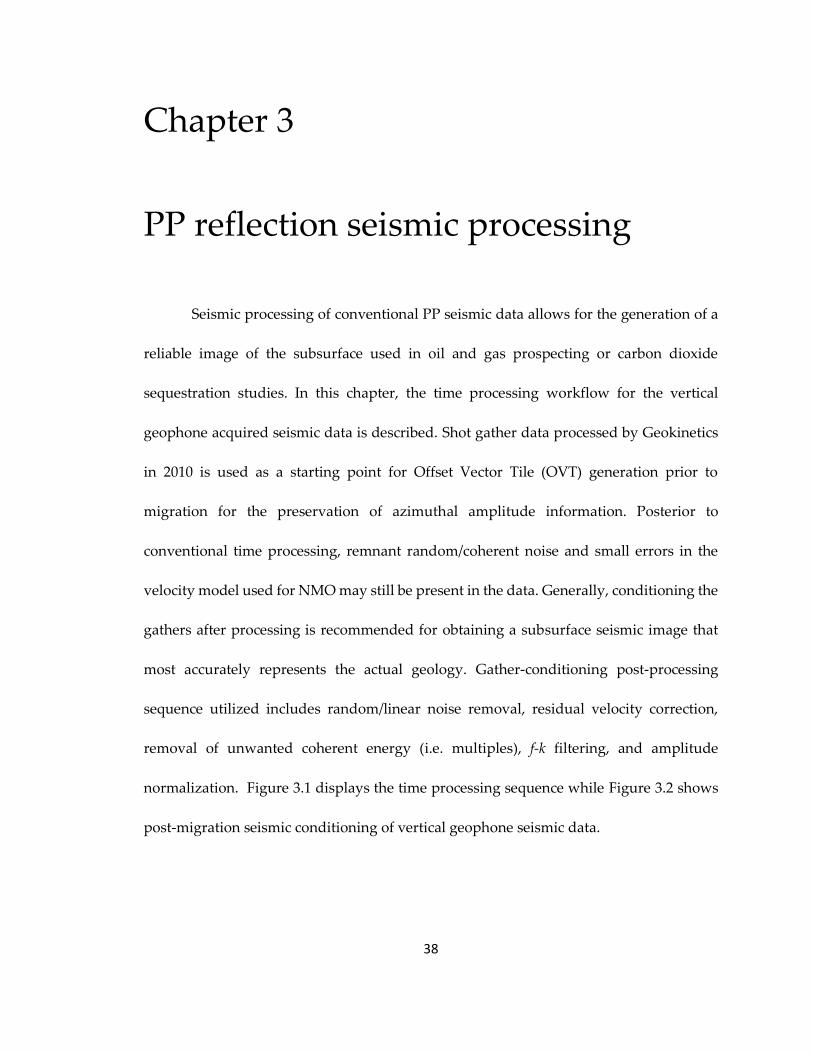
3. PP reflection seismic processing 38
3.1 PP seismic processing workflow.…………………………………………………….39
3.1.1 Time processing workflow…………………………………………………...39
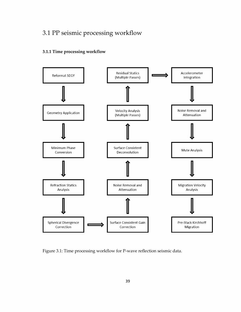
3.1.2 Gather-conditioning workflow……………………………………………....40
3.2 Offset vector tiles…………………………………………………………………….....40
3.2.1 OVT definition…………………………………………………………………40
3.2.2 Kirchhoff migration on OVTs………………………………………………..45
3.3 Gather-conditioning…………………………………………………………...………47
3.3.1 Structure-oriented filter…………………………………………...……….…47
3.3.2 VTI and HTI corrections……………………………………………………...49
3.3.3 Radon de-multiple………………………………………………………….....52
viii
3.3.4 CDP domain noise attenuation…………………………………………..…..55
4. AVO simultaneous inversion 58
4.1 Seismic – well correlation……………………………………………………………..60
4.1.1 Convolutional model……………………………………………………….…60
4.1.2 Wavelet and synthetic seismogram………………………………………….61
4.2 Angle stack generation………………………………………………………………...63
4.2.1 Angle range analysis……………………………………………………….....63
4.2.2 Angle stacks…………………………………………………………………....65
4.3 Wavelets………………………………………………………………………………...66
4.3.1 Wavelet extraction………………………………………………………….....66
4.4 Low-frequency background models generation………...……………………….....68
4.4.1 Collocated cokriging of well-logs……………………...…….……………....68
4.4.2 Low-frequency background models………………………………………...69
4.5 AVO inversion………………………………………………………………………….70
4.5.1 AVO inversion background………………………………………………….70
4.5.2 Parameters……………………………………………………………………..71
4.5.3 AVO inversion volumes……………………………………………………...72
4.5.4 Inversion QC……………………………………………………………….......73
5. PS reflections seismic processing and inversion 75
5.1 PS seismic processing……………………...…………………………………..............76
5.1.1 Processing workflow……………………………………………………….....75
ix
5.2 Statics……………………………….......………………………….................................77
5.2.1 Shear statics determination methods………………………………………..77
5.2.2 Shear-refraction picking…………………………………………………...….79
5.3 Velocity analysis………………………………………………………………………..82
5.3.1 Linear regression……………………………………………………………....82
5.3.2 Migration velocity analysis…………………………………………………..84
5.4 Processing…………………………………………………………………………….…86
5.4.1 Radial and transverse rotation……………………………………………….86
5.4.2 Converted-wave binning……………………………………………………..88
5.4.3 Kirchhoff migration…………………………………………………………...89
5.4.4 PP – PS event registration………………………………………………….…90
5.5 Shear post-stack inversion………………………………………………………...…..92
5.5.1 Shear well-to-seismic correlation………………………………………...…..92
5.5.2 Post-stack inversion……………………………………………………...……94
6. Interpretation 96
6.1 Porosity estimation……………………………………………………………….…....97
6.1.1 Linear regression………………………………………………………………97
6.1.2 Porosity volume……………………………………………………………….99
6.1.3 Porosity map…………………………………………………………….....…101
6.2 Attribute volumes………………………………………………………………….…102
6.2.1 and ……………………………………………………………………...102
x
6.2.2 Gradient and fluid factor………………………………………………...….103
6.2.3 Poisson’s ratio………………………………………………………………...105
6.2.4 Sweetness and spectral decomposition…………………….…………..….107
6.3 Azimuthal anisotropy analysis………………………………………………….…..110
6.3.1 Anisotropy magnitude…………………………………………………..…..110
6.3.2 Anisotropy magnitude and azimuth…………………………………..…..111
6.4 Volumetric analysis for CO2 sequestration………………………………………...113
6.4.1 Time-to-depth conversion…………...……………………………………...113
6.4.2 Isopach maps…………………………………………………………………114
6.4.3 Injection model and proposed well……………………………………...…116
6.4.4 Volumetric assessment……………………………………………………....118
6.4.5 CO2 chemical properties………………………………………………….…120
6.4.6 Injection analysis……………………………………………………………..123
7. Conclusions and future work 127
7.1 Conclusions………………………………………………………………………...….127
7.2 Future work……………………………………………………………………….…..136
References 137

xi
List of Figures
Figure 1.1: Schematic diagram demonstrating the typical process and depths for CCS.
(modified from EPA, 2017).………………..…………………...………………………………..5
Figure 1.2: Estimate of the goals of carbon dioxide that should be sequestered by the year
2050. A projection of the amount of CO2 from various CO2-emitting processes with time
is displayed (modified from IEA, 2013).…………………………………….………………….6
Figure 1.3: Map of CCS projects in North America for CO2 emitted from power plants.
Approximately 25 projects worldwide are currently operational. 13 projects are currently
operational in North America (modified from Burns, 2017).…..……………………………..7
Figure 1.4: Schematic diagram displaying an incident P-wave and its corresponding
reflected and refracted P and S-waves (modified from Feng and Bancroft, 2006).…...…..…8
Figure 1.5: Map location of Rock Springs Uplift, Sweetwater County, Wyoming, USA (left)
and the location of a seismic survey area (right) (modified from Mallick, 2015)……..……12
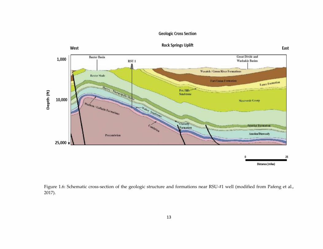
Figure 1.6: Schematic cross-section of the geologic structure and formations near RSU-#1
well (modified from Mallick, 2015).………………………………………..………………….13
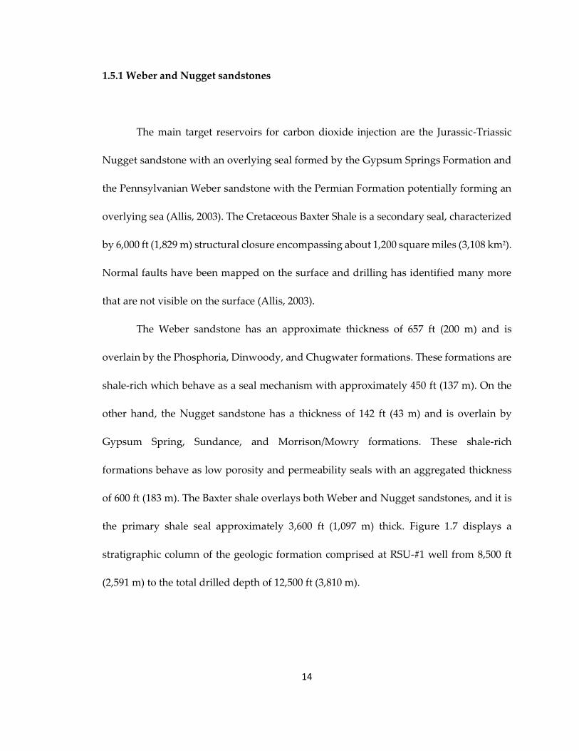
Figure 1.7 Stratigraphic column at RSU-#1 well from 9,000 ft (2,743 m) to total drilled
depth of 12,500 ft (3,810 m). Gamma-ray values are displayed for each formation
(modified from Mallick, 2015).…………………………………………….……….…...……...15
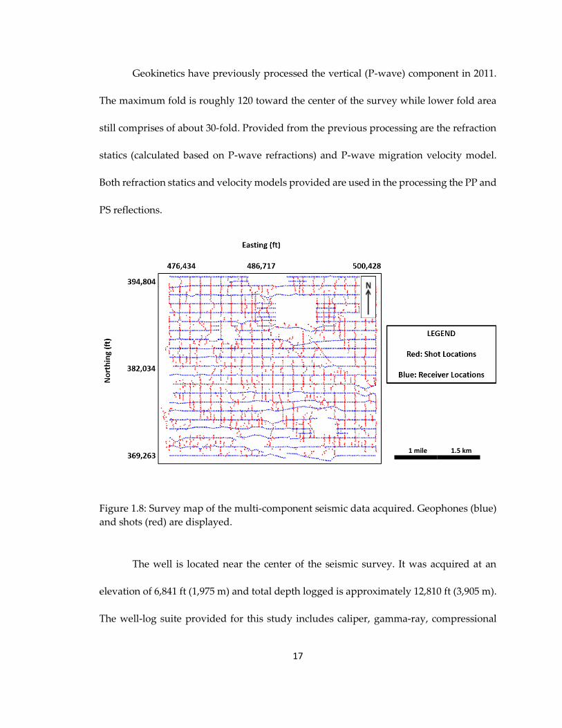
Figure 1.8: Survey map of the multi-component seismic data acquired. Geophones (blue)
and shots (red) are displayed.…………...……………………………………………….….…17

xii
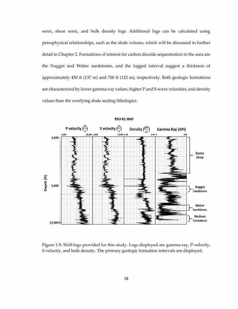
Figure 1.9: Well-logs provided for this study. Logs displayed are gamma-ray, P-velocity,
S-velocity, and bulk density. The primary geologic formation intervals are
displayed.…………………………………………………………………...…………………...18
Figure 2.1: vs. theoretical cross-plot defining areas for various lithologies and fluid
saturations (from Goodway et al., 1997).……………………………………………...…....…28
Figure 2.2: vs. at RSU-#1 well for the Nugget sandstone (left) and the Weber
sandstone (right). Values are within the 20% cut-off for high-porosity sandstones. Color
bar represents gamma-ray values scaled in American Petroleum Institute (API) units.….28
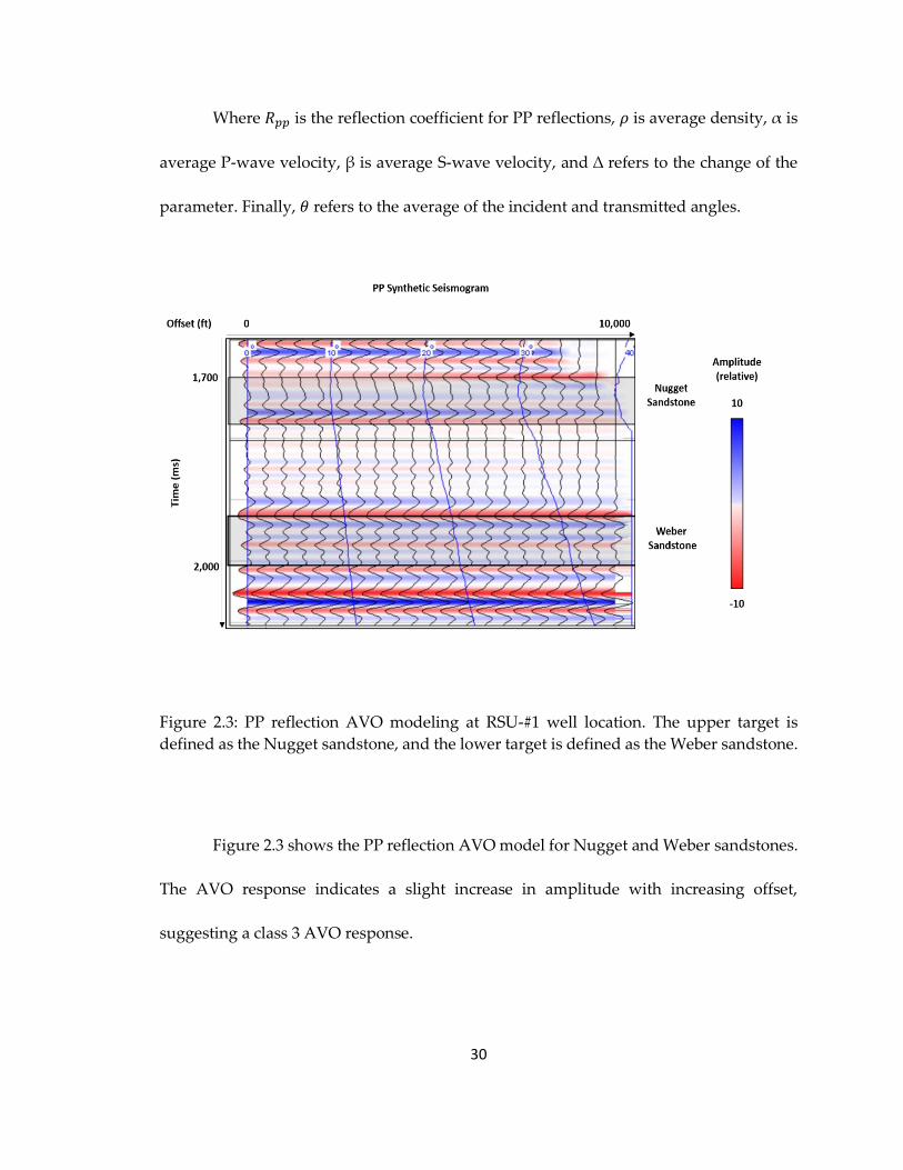
Figure 2.3: PP reflection AVO modeling at RSU-#1 well location. The upper target is
defined as the Nugget sandstone, and the lower target is defined as the Weber
sandstone………………………………………………………………………………………...30
Figure 2.4: PS reflection AVO modeling at RSU-#1 well location. The upper target is
defined as the Nugget sandstone, and the lower target is defined as the Weber
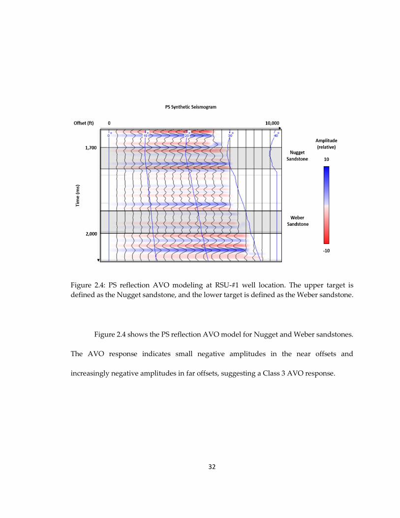
sandstone………………………………………………………………………………………...32
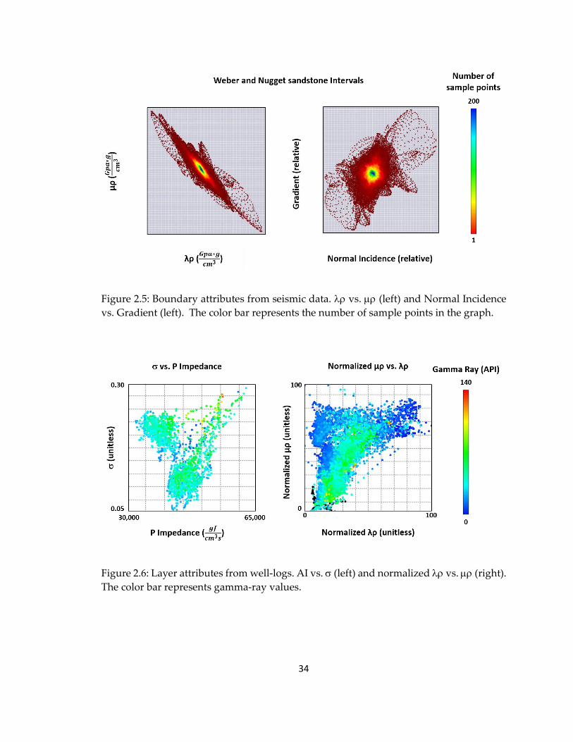
Figure 2.5: Boundary attributes from seismic data. vs. (left) and Normal Incidence
vs. Gradient (left). The color bar represents the number of sample points in the graph......34
Figure 2.6: Layer attributes from well-logs. AI vs. (left) and normalized vs. (right).
The color bar represents gamma-ray values………………………………………….………34
Figure 2.7: Rock physics relationships calculated for sensitivity analysis. Vp vs. Density
(left) and Vp vs. Porosity (right). The color bar represents gamma-ray values….…………35
Figure 2.8: Sensitivity analysis results for Vp, density, porosity, , and . Black curve
denotes in-situ logs, and red curves denote the logs with 5% porosity
increase…………………………………………………………………………..……………....37
Figure 3.1: Time processing workflow for P-wave reflection seismic data………………...39
xiii
Figure 3.2: Representation of the seismic gather-conditioning workflow………..……......40
Figure 3.3: Rose diagram of azimuth – offset distribution for the Jim Bridger 3D survey.
The color bar represents the fold number…………………………..…………………….…...42
Figure 3.4: Offset vector tiles (OVT) theoretical distribution. The color bar represents the
ring number…………………………………………………...………………………………....43
Figure 3.5: CDP gathers sorted as common offset and common azimuth to demonstrate
the effect of azimuthal velocity variations. COCA values range from 1,000 to 13,000 for
each CDP gather……………………..………………………………………………………….44
Figure 3.6: CDP gathers display for the Kirchhoff PSTM before (left) and after (right).
Offset ranges from 0 – 19,000 ft for each CDP gather……………………………….………...46
Figure 3.7: CDP gathers display for Structure-Oriented Filtering (SOF) before (left), after
(middle), and difference (right). Offset ranges from 0 – 19,000 ft for each CDP
gather…………………………...………………………………………………………..……....48
Figure 3.8: CDP gathers display for VTI/HTI velocity correction before (left) and after
(right). Offset ranges from 0 – 19,000 ft for each CDP gather……………………………..….50
Figure 3.9: P-wave interval velocity field before (left) and after (right) the HTI/VTI
anisotropic corrections……………………………………………………………………….....51
Figure 3.10: CDP gathers display for Radon de-multiple before (left), after (middle), and
difference (right). Offset ranges from 0 – 19,000 ft for each CDP gather…………………....54
Figure 3.11: CDP gathers display for CDP domain noise attenuation before (left), after
(middle), and difference (right). Offset ranges from 0 – 19,000 ft for each CDP gather…...56
xiv
Figure 3.12: Full stack section before (left) and after (right) post-migration seismic
conditioning.…………...………………………………………….………………………….…57
Figure 4.1: Schematic diagram defining the methodology for IFP’s pre-stack AVO
simultaneous inversion…………………………………………………………………….…..59
Figure 4.2: Schematic representation of a synthetic seismogram generated using the
convolutional model (modified from Russell, 2010)…...………………………………...…..60
Figure 4.3: Wavelet, spectrum, phase, and cross-correlation extracted at RSU-#1 well
location…………………………………………………………………………………………..61
Figure 4.4: Seismic-to-well correlation at RSU-#1 well location. Synthetic generated from
the well is overlain to compare to the seismic section amplitudes….…………………..…62
Figure 4.5: Angle range analysis on CDP gathers. Ray-traced incident angles are overlain
on the CDP gathers………………………………………………...…………………………....64
Figure 4.6: Angle stacks generated from the gathers using a ray-tracing technique. Angle
ranges are displayed for each angle stack….…………………………………………….........65
Figure 4.7: Wavelets and phase extracted from the angle stacks. The phase is roughly zero
phase for all angle stacks………………………………………………………………..……...67
Figure 4.8: P impedance (left), S impedance (middle), and density (right) high-cut filtered
background models……………………………………………………………………….….…69
Figure 4.9: P impedance, S impedance, and density inversion results at inline 118 with
log values overlay....……………………………………………………………………………72
xv
Figure 4.10: P impedance, S impedance, and density inversion QC cross-plots. The x-axis
corresponds to the well-log and y-axis to the inversion extracted at RSU-#1 well location.
The color bar represents the number of sample points in the cross-plot…………...……..73
Figure 4.11: P impedance, S impedance, and density logs (black), background models
(green), and inversion (red) overlay extracted at RSU-#1 well location for QC………….74
Figure 5.1: Representation of the PS processing workflow….……………………………....76
Figure 5.2: Shot (left) and receiver (right) refraction statics map determined from PP
refraction events..……………………………………………………………………………….78
Figure 5.3: A shot gather with refraction statics picking. Manual picks (pink) done for an
offset range of 3,000 ft (914.4 m) to 8,000 ft (2,438 m)...……………………………………….80
Figure 5.4: Cross-section for the north-south and east-west directions, displaying
velocity values from refraction picks…...………………………………………….................80
Figure 5.5: Delay time map in milliseconds from the shear-refraction statics solution.....81
Figure 5.6: Vp
Vs cross-plot utilized for the linear regression generation. The color bar
represents the number of sample points in the cross-plot………………………………….83
Figure 5.7: Vp migration velocities from PP processing and Vp
Vs field volume calculated
from the linear regression………………………………..………………………………….....83
Figure 5.8: Migration velocity analysis demonstrated from velocity picks from
semblance analysis (left) and migrated stack response (right)....……………………….....85
xvi
Figure 5.9: Schematic diagram displaying radial and transverse directions along with
acquisition shot and receiver lines, H1 and H2 (from Grossman and Popov, 2014)….....86
Figure 5.10: Converted-wave CDP gathers for X and Y components before and after
rotation to its corresponding radial and transverse. Offset ranges from 0 – 19,000 ft for
each CDP gather……………………………………...…………………………………………87
Figure 5.11: Schematic diagram showing the CMP, CCP, and ACP coordinates for a
source and receiver pair (modified from Tessmer and Behle, 1988)….………………...…88
Figure 5.12: Display of converted-wave stack before (left) and after (right) the Kirchhoff
migration and residual statics are applied…………………………………………………...89
Figure 5.13: Display of stack before (left) and after (right) the event registration….....…90
Figure 5.14: Comparison of the PP stack and PS stack after the event registration in PP
time. The Nugget sandstone, Weber sandstone, and Madison limestone tops are
annotated…………………………………………………………………………...…………....91
Figure 5.15: Well-to-seismic correlation for the converted-wave stack at the RSU-#1
location…………………………………………………………………………………………..92
Figure 5.16: Extracted wavelet, spectrum, phase for the converted-wave seismic stack at
the RSU-#1 well location….……………………………………………………………………93
Figure 5.17: Shear impedance volume generated from the converted-wave seismic
section. Shear impedance inversion volume is displayed at the well RSU-#1 location.....95
Figure 6.1: Linear regression analysis from well attributes. Porosity vs. density (left) and
porosity vs. (right).…………………………………………………………………………..98
xvii
Figure 6.2: Porosity section derived by applying the porosity – transform to the
volume from the AVO inversion. Top and base of the Nugget and Weber sandstone
horizons are displayed………………………………………………………………………….99
Figure 6.3: Porosity section derived by applying the porosity – transform to the
volume from the PS post-stack inversion. Frontier shale, Nugget and Weber sandstones,
and Madison limestone horizons are displayed…...……………………………………......100
Figure 6.4: Porosity maps extracted from top to base of the formation for the Nugget
sandstone (left) and the Weber sandstone (right). ……….……………………………..…..101
Figure 6.5: and map for the Nugget sandstone interval…….…………………….…102
Figure 6.6: Gradient (left) and fluid factor (right) RMS maps for Weber sandstone
formation.………………………………………………………………………………………104
Figure 6.7: Poisson’s ratio RMS map extracted for the interval of the Nugget
sandstone…………………………………………………………………………………...…..106
Figure 6.8: Sweetness attribute RMS map extracted for Nugget and Weber sandstone
interval………………………………………………………………………………………….108
Figure 6.9: Spectral decomposition for 10, 20, 30 Hz for the Nugget and Weber sandstones,
respectively..….………………………………………………………………………………..109
Figure 6.10: Magnitude of anisotropy maps extracted for the Nugget and Weber
sandstones……...………………………………………………………………………………110
Figure 6.11: Anisotropic vector maps delineating fracture orientation for the Nugget and
Weber sandstones………………………...…………………………………………………....111

xviii
Figure 6.12: Regional stress map for the location for the area of study displaying direction
of regional stress field from geologic measurements (modified from WSM, 2016)….......112
Figure 6.13: Time (left) to depth (right) conversion example from the P impedance
volume………………………………………………………………………………………….113
Figure 6.14: Thickness maps for the Nugget and Weber sandstones…………………….114
Figure 6.15: Top and base horizon depth maps for the Nugget and Weber sandstones…115
Figure 6.16: Extracted porosity map for the Nugget and Weber sandstones, displaying
the location for the planned well (CCS-#1 well) for carbon dioxide sequestration…......116
Figure 6.17: Chair display of seismic data at the location of the proposed well. The
Nugget and Weber horizons are displayed………………………………………………...117
Figure 6.18: High porosity maps for the Nugget and Weber sandstones, demonstrating
high, middle, and low probabilities of obtaining a high-porosity anomaly for CCS …....119
Figure 6.19: Geothermal (right) and lithostatic pressure (left) gradients for the subsurface
(modified from Sclater et al., 1980; Schlumberger Oilfield Glossary, 2019)…….....…..….121
Figure 6.20: Phase diagram for carbon dioxide (modified from Global CCS Institute,
2019)…………………………………………………………………………………………….122
Figure 6.21: A schematic diagram of a CO2 storage site demonstrating the principles of
available space, used space, spill point, affected space, and unaffected space (from van der
Meer, 2008)……………………………………………………………………………………..124
xix
List of Tables
Table 1.1: Acquisition parameters for the Jim Bridger 3D seismic survey (modified from
Mallick, 2015)……………………………………………………………….………………..….16
Table 2.1: List of layer and boundary attributes analyzed in this study..………………......33
Table 3.1: Parameters used for the Kirchhoff Pre-stack Time Migration (PSTM)…….….45
Table 3.2: Parameters used for the Structure-Oriented Bilateral Filtering (SOF)…...……...47
Table 3.3: Parameters used for the VTI and HTI velocity corrections……………………....50
Table 3.4: Parameters (right) and polygon mute (left) in - domain for Radon de-
multiple…………………………………………………………………………………………..53
Table 3.5: Parameters for the f-k filter (right) and the Radon de-noise polygon mute
(left)……………………………………………………………………………………………....56
Table 4.1: Parameter list for the generation of the low-frequency background models and
AVO inversion volumes………………………………………………………………………..71
Table 6.1: Estimated carbon dioxide mass for storage capacity in Mt…………………...118
Table 6.2: Estimated carbon dioxide mass for storage capacity in Mt considering the
storage capacity factor………………………………………………………………...……....126

xx
Table 6.3: Estimated duration for carbon dioxide sequestration in years from the Jim
Bridger power plant…………...………………………………………………………………126
xxi
List of Abbreviations
ACP = Asymmetrical Conversion Point
AI = Acoustic Impedance
AVA = Amplitude Versus Azimuth
AVO = Amplitude Versus Offset
CCP = Common Conversion Point
CCS = Carbon Capture and Sequestration
CDP = Common Depth Point
CMP = Common Mid-Point
CO2 = Carbon Dioxide
DHI = Direct Hydrocarbon Indicator
f-k = Frequency – Wavenumber
ft = Feet
ft/s = Feet per Second
G = Gradient
GR = Gamma-Ray

xxii
HTI = Horizontal Transverse Isotropy
Hz = Hertz
IFP = Institut Francais du Petrole
NMO = Normal Move Out
NI = Normal Incidence
m = Meters
mD = Millidarcy
ms = Milliseconds
Mt = Metric Megaton
m/s = Meters per Seconds
OVT = Offset Vector Tile
p = Move-Out
PR = Poisson’s Reflectivity
PP = Primary to Primary reflections
PS = Primary to Secondary reflections
PSTM = Pre-Stack Time Migration
RMS = Root Mean Square
xxiii
RNMO = Residual Normal Move Out
RSU = Rock Springs Uplift
s = Seconds
SI = Shear Impedance
SOF = Structure-Oriented Filter
SWS = Shear-wave Splitting
Vp = P velocity
Vs = S velocity
VTI = Vertical Transverse Isotropy
WAZ = Wide-Azimuth
= Density
= Porosity
= Poisson’s ratio
= Lambda-Rho
= Mu-Rho
Vp
Vs = P velocity over S velocity ratio
- = Two-way zero offset time – Ray parameter
1
Chapter 1
Introduction
Primary objectives of seismic exploration are to characterize the response of
seismic amplitudes and generate rock physics relationships that can be used to predict
variations in reservoir properties. The data may undergo a rigorous processing and post-
migration conditioning workflow that aids in the subsurface structural imaging and
increases signal-to-noise values to correctly characterize the subsurface via seismic
amplitudes. The results of seismic imaging can be utilized for the evaluation of seismic
amplitudes for reservoir characterization using various analytic interpretation
techniques such as forward modeling, sensitivity analysis, rock physics relationship
generation, AVO inversion, and elastic attribute interpretation. Even though often
ignored, the addition of converted-wave (PS) seismic data into the reservoir
characterization can significantly improve the determination of bulk density, which in
turns aids in the completeness of the reservoir studies. Joint PP-PS inversion
methodologies increase the reliability of elastic properties generated and can be used for
enhanced characterization of the subsurface.
2
1.1 The problem
Even though the subsurface of Rock Springs Uplift (RSU), Wyoming has been
subject to geologic analysis utilizing seismic data (Pafeng et al., 2017; Grana et al., 2017),
a more robust reservoir characterization can be employed to obtain reliable information
of porosity, density, and elastic rock properties by incorporating PS converted seismic
wave data to the analysis. Although it is widely known the incorporation of converted-
wave data to reservoir analysis can aid in the reliable determination of elastic properties,
this type of dataset is often neglected in the oil and gas industry (Pafeng et al., 2017). PP
reflection data is dependent on the rock matrix and the saturating fluid within the rock
matrix. Although this may be beneficial for characterizing hydrocarbons in oil and gas
exploration, additional information is required to obtain information solely on the rock
medium in which the wave propagates. Fluids lack the ability to resist shear stresses, and
the primary driving mechanism of shear-wave propagation is through shear resistance
(Omnes, 1978). Hence, the S-wave largely neglects the saturating fluid and is primarily
affected by the rock matrix. Thus, elastic rock properties can be extracted for reservoir
analysis with increased accuracy in comparison to attributes generated solely based on
PP data.
3
1.2 Objectives
This study aims to investigate the rock properties of the Pennsylvanian Weber
and Jurassic – Triassic Nugget sandstones in the Rock Springs Uplift, Wyoming and
create rock physics relationships with the elastic response. Seismic processing, forward
modeling, and sensitivity analysis are carried out with the primary purpose of finding a
signature of the porosity and elastic behavior of the reservoir of interest. Furthermore, PS
converted-wave seismic data are incorporated in the study to aid the characterization of
the elastic response from the derivation of rock properties. This is undertaken via PP and
PS seismic inversion followed by a robust multi-attribute interpretation process
conducted to estimate accurate porosity values utilized for CO2 storage. The results from
the inversion are used to develop additional elastic attributes that are used to identify
lithologic and geomechanical information of the Weber and Nugget sandstones.
The main questions to address in this study are:
- What rock physics relationships can be derived from well-logs to
determine accurate elastic property characteristics using seismic data?
- Where are the locations with higher porosity content for the Nugget
and Weber sandstones for CO2 storage within the seismic survey?
- What are the multicomponent processing and gather-conditioning
workflows and parameters for the seismic data in this area? (i.e. statics,
velocity models).
4
1.3 Carbon dioxide sequestration
Carbon capture storage or sequestration (CSS) refers to the capturing of CO2 by
utilizing industrial plants to remove the CO2 from exhaust gases and potentially use deep
strata within the subsurface for long-term storage away from the atmosphere (Benson
and Cole, 2008). This process requires the compression and injection of the CO2 in sealed
and porous sedimentary compartments within geologic formations, where it can
potentially remain stored for long periods of time. The principal strata of interest for CCS
are thick sequences of sedimentary rocks within which there are permeable rocks such as
sandstones, which work as storage reservoirs. Overlying low permeability rocks,
typically shales, serve as seals to block upward migration of the CO2 (Benson and Cole,
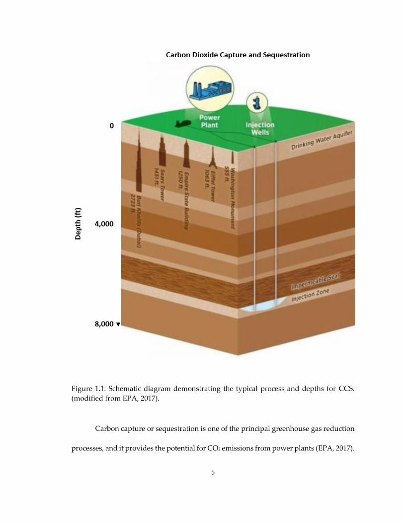
2008). Figure 1.1 displays the typical process for CCS and the expected depths of
sequestration.
The main goal of storing CO2 in deep sedimentary formations is to diminish
emissions of greenhouse gases into the atmosphere. A billion metric tons or more must
be sequestered annually to noticeably reduce CO2 in the atmosphere (Benson and Cole,
2008). This corresponds to 250 times increase over the amount of what is sequestered
today. CCS contributes up to 20% of carbon dioxide emissions reduction (Benson and
Cole, 2008).
5
Figure 1.1: Schematic diagram demonstrating the typical process and depths for CCS.
(modified from EPA, 2017).
Carbon capture or sequestration is one of the principal greenhouse gas reduction
processes, and it provides the potential for CO2 emissions from power plants (EPA, 2017).
6
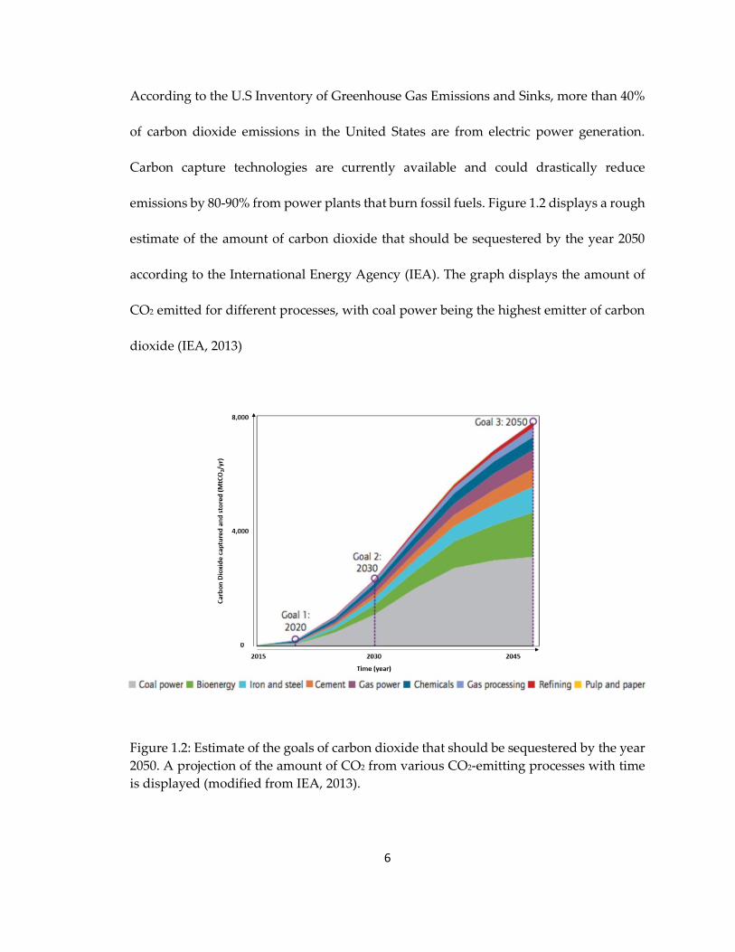
According to the U.S Inventory of Greenhouse Gas Emissions and Sinks, more than 40%
of carbon dioxide emissions in the United States are from electric power generation.
Carbon capture technologies are currently available and could drastically reduce
emissions by 80-90% from power plants that burn fossil fuels. Figure 1.2 displays a rough
estimate of the amount of carbon dioxide that should be sequestered by the year 2050
according to the International Energy Agency (IEA). The graph displays the amount of
CO2 emitted for different processes, with coal power being the highest emitter of carbon
dioxide (IEA, 2013)
Figure 1.2: Estimate of the goals of carbon dioxide that should be sequestered by the year
2050. A projection of the amount of CO2 from various CO2-emitting processes with time
is displayed (modified from IEA, 2013).
7
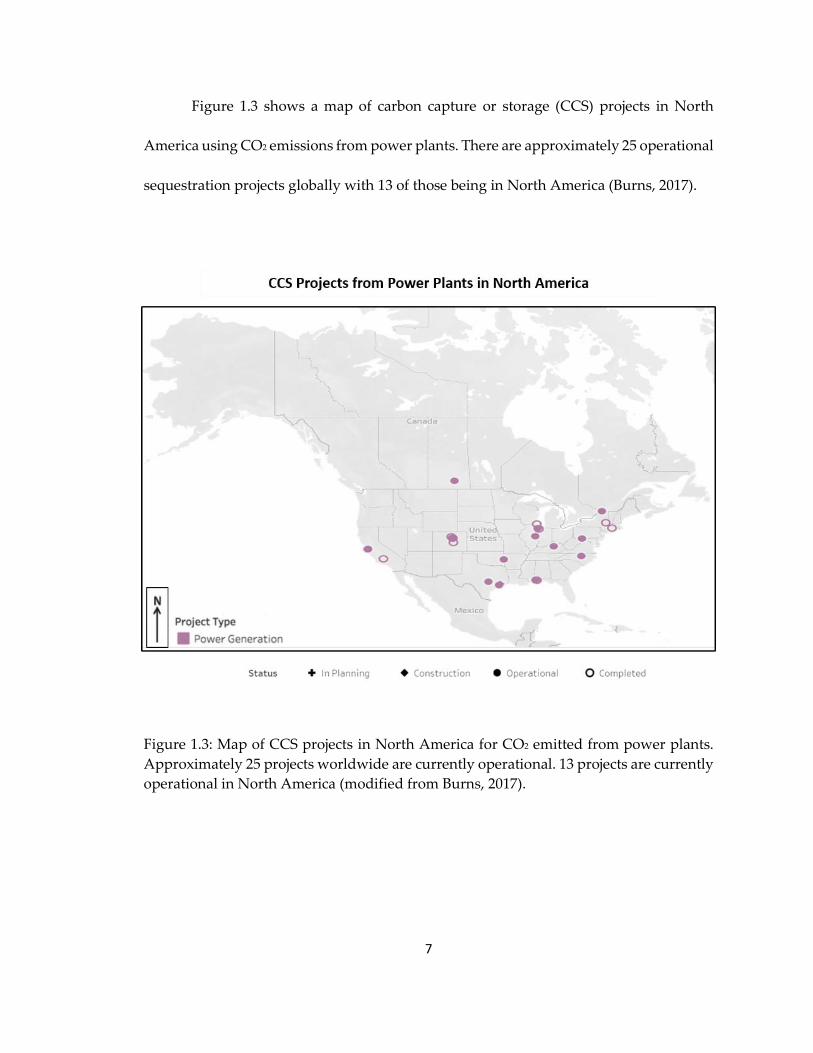
Figure 1.3 shows a map of carbon capture or storage (CCS) projects in North
America using CO2 emissions from power plants. There are approximately 25 operational
sequestration projects globally with 13 of those being in North America (Burns, 2017).
Figure 1.3: Map of CCS projects in North America for CO2 emitted from power plants.
Approximately 25 projects worldwide are currently operational. 13 projects are currently
operational in North America (modified from Burns, 2017).
8
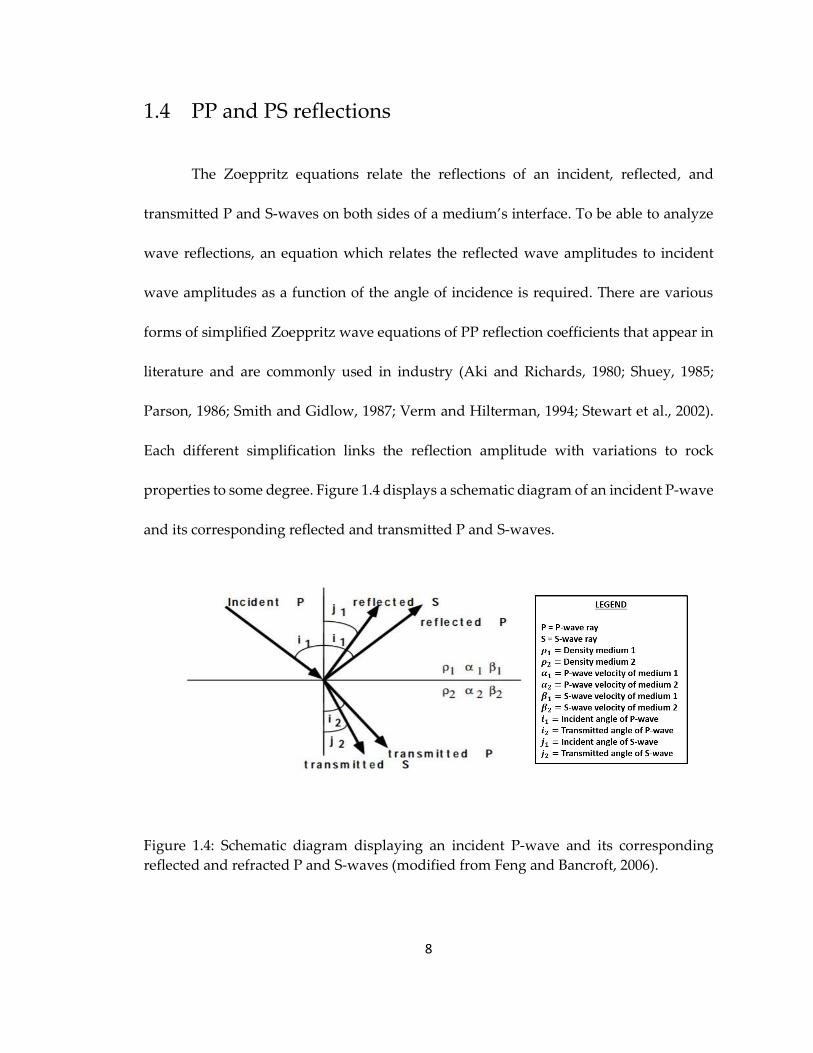
1.4 PP and PS reflections
The Zoeppritz equations relate the reflections of an incident, reflected, and
transmitted P and S-waves on both sides of a medium’s interface. To be able to analyze
wave reflections, an equation which relates the reflected wave amplitudes to incident
wave amplitudes as a function of the angle of incidence is required. There are various
forms of simplified Zoeppritz wave equations of PP reflection coefficients that appear in
literature and are commonly used in industry (Aki and Richards, 1980; Shuey, 1985;
Parson, 1986; Smith and Gidlow, 1987; Verm and Hilterman, 1994; Stewart et al., 2002).
Each different simplification links the reflection amplitude with variations to rock
properties to some degree. Figure 1.4 displays a schematic diagram of an incident P-wave
and its corresponding reflected and transmitted P and S-waves.
Figure 1.4: Schematic diagram displaying an incident P-wave and its corresponding
reflected and refracted P and S-waves (modified from Feng and Bancroft, 2006).
9
Amplitude versus offset or azimuth (AVO or AVA) equations describe the
amplitude coefficients of an incident P-wave as the angle of the incident or source-
receiver offsets increases. As the AVO phenomena translate the sharing of the energy of
the incident compressible wave between the compressible and converted reflections, the
observation of the converted mode AVO would be redundant (Xu and Bancroft, 1997.
Single fold data are not pure enough to provide reliable amplitude measurements and
results may be doubtful (Xu and Bancroft, 1997). In such a case, the study of AVO of the
converted-waves can be advantageous (Xu and Bancroft, 1997). Equation 1 displays the
Aki-Richards (1980) approximation of PS reflection coefficients.
𝑃𝑆 =−𝑝𝛼
2𝑐𝑜𝑠𝑗[(1 − 2𝛽2𝑝2 + 2𝛽2
𝑐𝑜𝑠𝑖
𝛼
𝑐𝑜𝑠𝑗
𝛽)
∆𝑝
𝑝− (4𝛽2𝑝2 − 4𝛽2
𝑐𝑜𝑠𝑖
𝛼
𝑐𝑜𝑠𝑗
𝛽)
∆𝛽
𝛽] (1)
Where 𝑃𝑆 refers to the reflection coefficient for converted-waves, 𝑝 is the average
density, 𝛼 is the average P-wave velocity, 𝛽 is the average S-wave velocity, and ∆ refers
to the change of the parameter. The angle 𝑖 is the average of the incident and transmitted
P-wave angles while 𝑗 is the average of the reflected and transmitted S-wave angles (Xu
and Bancroft, 1997). Although AVO analysis and methodologies are industry standard,
AVO assumes the recorded seismic data consists of primary reflections only and are not
contaminated by other wave propagation effects, such as multiples and converted-waves
(Pafeng et al., 2017). In a modeling study, Mallick and Adhikari (2015) demonstrate that
such assumptions are valid only for a relatively small source-to-receiver offset. Typically
for the offsets corresponding to the incident angles of 30 degrees or less. For the large
10
offsets or angles (greater than 30 degrees), the recorded seismic data are increasingly
affected by the complex effects of wave propagation; therefore, the application of AVO
to large offset/angle reflections become more difficult (Mallick and Adhikari, 2015).
A primary objective of pre-stack seismic inversion is to derive reliable estimates
of P-wave velocity, S-wave velocity, and density from which elastic attributes can be
calculated to predict fluid and lithologic properties of the subsurface. Due to limitations
of seismic methods such as band-limited characteristics and noise levels, information
from various approaches, such as converted-waves, are continuously obtained for a
comprehensive interpretation of the subsurface. P and S-wave velocities can be derived
from inversion and converted to and elastic attributes to detect reservoirs. They can
be used as direct hydrocarbon indicators (DHI) (Goodway et al., 1997). One of the main
issues of the seismic inversion is the non-uniqueness component due to the limited
information available. There are many sources of uncertainty such as errors in
background velocity that causes the Vp
Vs to change significantly and eliminates the high-
frequency contrast. Careful selection of parameters, background velocity, wavelet
estimation, and application of a priori information is still important issues which remain
to be resolved (Xu and Bancroft, 1997). By incorporating additional information to the
seismic inversion, such as PS reflection data, the inversion becomes more stable and more
reliable results from elastic attributes can be obtained.

11
1.5 Geological background
The Rock Springs Uplift (RSU) was formed during the late Cretaceous to
Paleogene Laramide Orogeny, and it is cut by several east and north-east trending faults
(Erslev and Koenig, 2009) located in Sweetwater County, Wyoming (Figure 1.5). The
uplift extends for approximately 50 miles (80 km) in the north-south direction and 35
miles (56 km) in the east-west direction and is characterized by a plunging anticline
structure (Mallick and Adhikari, 2015). The Baxter shale is the secondary seal above the
primary target formations for this study, which are the Weber and Nugget sandstones.
The Mesa Verde group is 3,500 ft (1,066 m) thick and overlays the Baxter Shale. This
geologic group consists of, in ascending order, the Blair formation, Rock Springs
formation, Ericson sandstone, and Almond formation (Mallick and Adhikari, 2015). A
thick Paleozoic deep saline aquifer sequence; Madison limestone and Weber sandstone
are overlain by sealing shale formations (Mowry and Baxter shales and the Lower
Triassic units). These aquifers, in conjunction with the quality of the overlying seals,
make them potential targets for CO2 sequestration (McLaughlin and Garcia-Gonzales,
2013).
The geologic setting at RSU contains favorable characteristics for potential CO2
sequestration. This includes laterally extensive sandstone reservoirs, primary seals
directly overlying the potential reservoirs, and a thick secondary seal (Allis, 2003).
Figure 1.6 displays a schematic cross-section of the geologic structure and formations
near the well RSU-#1.

12
Figure 1.5: Map location of Rock Springs Uplift, Sweetwater County, Wyoming, USA (left) and the location of a seismic survey
area (right) (modified from Mallick and Adhikari, 2015).
1.5 km 1 mile
13
Figure 1.6: Schematic cross-section of the geologic structure and formations near RSU-#1 well (modified from Pafeng et al.,
2017).
14
1.5.1 Weber and Nugget sandstones
The main target reservoirs for carbon dioxide injection are the Jurassic-Triassic
Nugget sandstone with an overlying seal formed by the Gypsum Springs Formation and
the Pennsylvanian Weber sandstone with the Permian Formation potentially forming an
overlying sea (Allis, 2003). The Cretaceous Baxter Shale is a secondary seal, characterized
by 6,000 ft (1,829 m) structural closure encompassing about 1,200 square miles (3,108 km2).
Normal faults have been mapped on the surface and drilling has identified many more
that are not visible on the surface (Allis, 2003).
The Weber sandstone has an approximate thickness of 657 ft (200 m) and is
overlain by the Phosphoria, Dinwoody, and Chugwater formations. These formations are
shale-rich which behave as a seal mechanism with approximately 450 ft (137 m). On the
other hand, the Nugget sandstone has a thickness of 142 ft (43 m) and is overlain by
Gypsum Spring, Sundance, and Morrison/Mowry formations. These shale-rich
formations behave as low porosity and permeability seals with an aggregated thickness
of 600 ft (183 m). The Baxter shale overlays both Weber and Nugget sandstones, and it is
the primary shale seal approximately 3,600 ft (1,097 m) thick. Figure 1.7 displays a
stratigraphic column of the geologic formation comprised at RSU-#1 well from 8,500 ft
(2,591 m) to the total drilled depth of 12,500 ft (3,810 m).
15
Figure 1.7 Stratigraphic column at RSU-#1 well from 9,000 ft (2,743 m) to total drilled
depth of 12,500 ft (3,810 m). Gamma-ray values are displayed for each formation (modified from Pafeng et al., 2017).
16
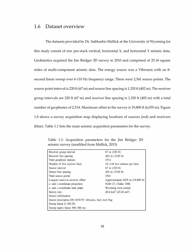
1.6 Dataset overview
The datasets provided by Dr. Subhashis Mallick at the University of Wyoming for
this study consist of raw pre-stack vertical, horizontal X, and horizontal Y seismic data.
Geokinetics acquired the Jim Bridger 3D survey in 2010 and comprised of 25.16 square
miles of multi-component seismic data. The energy source was a Vibroseis with an 8-
second linear sweep over 6-110 Hz frequency range. There were 2,541 source points. The
source point interval is 220 ft (67 m) and source line spacing is 1,320 ft (402 m). The receiver
group intervals are 220 ft (67 m) and receiver line spacing is 1,320 ft (402 m) with a total
number of geophones of 2,514. Maximum offset in the survey is 19,800 ft (6,035 m). Figure
1.8 shows a survey acquisition map displaying locations of sources (red) and receivers
(blue). Table 1.1 lists the main seismic acquisition parameters for the survey.
Table 1.1: Acquisition parameters for the Jim Bridger 3D
seismic survey (modified from Mallick, 2015)
17
Geokinetics have previously processed the vertical (P-wave) component in 2011.
The maximum fold is roughly 120 toward the center of the survey while lower fold area
still comprises of about 30-fold. Provided from the previous processing are the refraction
statics (calculated based on P-wave refractions) and P-wave migration velocity model.
Both refraction statics and velocity models provided are used in the processing the PP and
PS reflections.
Figure 1.8: Survey map of the multi-component seismic data acquired. Geophones (blue)
and shots (red) are displayed.
The well is located near the center of the seismic survey. It was acquired at an
elevation of 6,841 ft (1,975 m) and total depth logged is approximately 12,810 ft (3,905 m).
The well-log suite provided for this study includes caliper, gamma-ray, compressional
1.5 km 1 mile
18
sonic, shear sonic, and bulk density logs. Additional logs can be calculated using
petrophysical relationships, such as the shale volume, which will be discussed in further
detail in Chapter 2. Formations of interest for carbon dioxide sequestration in the area are
the Nugget and Weber sandstones, and the logged interval suggest a thickness of
approximately 450 ft (137 m) and 700 ft (123 m), respectively. Both geologic formations
are characterized by lower gamma-ray values, higher P and S-wave velocities, and density
values than the overlying shale sealing lithologies.
Figure 1.9: Well-logs provided for this study. Logs displayed are gamma-ray, P-velocity,
S-velocity, and bulk density. The primary geologic formation intervals are displayed.
19
1.6.1 Software
The well-log analysis and seismic modeling are carried out using Jtips™
developed by Dr. Fred Hilterman at the University of Houston. For the seismic processing
and post-migration conditioning, Ethos processing platform is used, a software currently
owned by SAExploration. For the pre-stack simultaneous AVO inversion and elastic
attribute interpretation, Paradigm software is used. Additional seismic attributes such as
sweetness and spectral decomposition are generated utilizing Transform by Drilling Info.
20
Chapter 2
Well-log analysis and AVO seismic
modeling
The well-logs available at RSU#1 well are used to further investigate the
mechanical and petrophysical properties of formations of interest, to obtain relationships
of petrophysical properties with elastic parameters in the subsurface. Relationships
between the rock properties and the elastic/acoustic response are evaluated and forward
models generated from P-wave velocity, S-wave velocity, and density to aid the
understanding of the seismic amplitude response of the area.
Petrophysical analysis of the available well-logs aid in the study of the data. Prior
to the evaluation of the logs, QC and editing are done to validate the correctness of the
data acquired at each interval. The evaluation comprises of an analysis of the target
intervals to estimate sand and shale volume percentage, porosity, P-wave velocity, S-
wave velocity, , among other attributes. A log of Vp
Vs is calculated which aids in the
generation of the S-wave velocity volume in the multi-component processing stage.
Additionally, to further analyze the petrophysical, geomechanical, and elastic properties
21
of the formations of interest, relationships are generated by cross-plotting any given rock
property (i.e. porosity vs. ) and deriving a least-squares regression. Such relationships
are utilized in the interpretation stage for the assessment of carbon dioxide sequestration.
Subsequently, the Amplitude Versus Offset (AVO) modeling phase of the project
comprises of synthetic models generated from log data by forward modeling the elastic
response of the amplitudes due to the geology in the subsurface. Along with the
petrophysical evaluation of the data, wavelets are extracted from seismic, AVO models
are generated, and sensitivity analysis in terms of porosity is done to understand the
elastic models that accurately represent the area of evaluation. Synthetic models obtained
from AVO studies are typically CDP gathers that vary with offsets with or without NMO
correction. Such AVO models can be generated for PP and PS reflections, which are
compared to the multi-component data. The forward models are calculated using a ray-
tracing method or finite difference/element wave-equation methods. The accuracy of the
models, computation power, and time depend on the approach chosen for the AVO model
generation.

22
2.1 Petrophysics
2.1.1 Log editing
The role of petrophysics in seismic interpretation has taken a significant leap
forward in the past ten years, resulting from essential advances in seismic data processing
techniques, particularly seismic inversion, attribute analysis, and amplitude versus offset
methods that showed we could estimate reservoir properties from such data (Crain, 2003).
Seismic petrophysics is a term used to describe the conversion of seismic data into
meaningful petrophysical or reservoir description information, such as porosity,
lithology, or fluid content of the reservoir (Crain, 2003). Until recently, this work was
qualitative, but as seismic acquisition and processing have advanced, the results are
becoming more quantitative. Calibrating this work to well-log “ground truth” can convert
the seismic attributes into useful reservoir exploration and development tools. Since there
is an infinite number of possible inversions, it is significant to find the one that most
closely matched the final edited logs or the computed results from those logs (Crain, 2003).
Geophysical well-logs suffer from many borehole and environmental problems
that need to be repaired before being used for calibrating seismic models or seismic
interpretations (Crain, 2003). The first step prior to geophysical analysis is the quality
control (QC) of well data by ensuring the data does not suffer from incorrect measurement
readings, wash-outs, spikes, and anomalies. Such inaccurate information may display
non-geologic responses while analyzing reservoir, characteristics such as lithology, fluid
23
saturation, and porosity. After such log anomalies are located and corrected within the
well-log, petrophysical relationships can be applied to the logs available to obtain
additional geophysical properties. The logs calculated in this study include, but not
limited to, Vp
Vs, , sand volume, and elastic attributes, and porosity.
2.1.2 𝐕𝐩
𝐕𝐬 and
Compressional and shear sonic logs are measurements of P and S-wave slowness
for a given lithologic formation in the subsurface. Such measurements are inversely
related to the P and S-wave velocities, respectively; thus, a Vp
Vs can be derived by dividing
Vp by Vs obtained from sonic well measurements. Typical values range from 1.4 – 3.0 and
can be indicative of fluid saturation due to the S-wave’s insensitivity to fluid or porosity
due to P-wave’s velocity decrease with increased porosity. The Weber and Nugget
sandstones have values of 1.71 – 1.85 which indicate a stiffer lithology. The sealing shale
lithologies beneath the target sandstones display values of 1.84 – 1.96. An additional log
calculated that aids in the characterization of the reservoir is the and is directly related
to the Vp
Vs.
24
Values of typically range between 0 – 0.5 in rocks. The Weber and Nugget
sandstones display values of 0.06 and 0.15; meanwhile, the sealing shale beneath has
values of 0.24 and 0.37.
2.1.3 Sand volume and porosity
In reservoir characterization studies, it is imperative to characterize the rock by
lithologic composition. In siliciclastic reservoir plays, the target sandstones can be
analyzed for sandstone and shale percentages in composition. Wave propagation through
rock siliciclastic media is heavily influenced by the number of clay compounds in shale
strata; thus, to confidently characterize the seismic response, the differentiation between
sands and shales is one of the main objectives in a petrophysical analysis.
Gamma-ray (GR) logging is a standard and inexpensive measurement of the natural
emission of gamma-rays by a formation. GR logs are particularly helpful because shales
and sandstones typically have different gamma-ray signatures that can be correlated
readily between wells (Schlumberger Oilfield Glossary, 2019). GR is a log of the total
natural radioactivity measured in API units. The measurement can be made in both open-
hole and through the casing. The depth of investigation is a few inches so that the log
usually measures the flushed zone. Shales and clays are responsible for most natural
radioactivity, so the gamma-ray log often is a good indicator of such rocks (Schlumberger
Oilfield Glossary, 2019). Shale is usually more radioactive than sand or carbonate. The
25
gamma-ray log can be used to calculate the volume of shale in porous reservoirs. The
volume of shale expressed as a decimal fraction or percentage is called Vsh (Saputra, 2008).
The GR log has several nonlinear empirical responses as well as linear responses. The non-
linear responses are based on geographic area or formation age. All non-linear
relationships are more optimistic. That is, they produce a shale volume value lower than
that from the linear equation (Saputra, 2008). Equation 2 can be used to determine the
volume of shale facies by comparing the minimum and maximum baseline gamma-ray
values for such facies with the current GR log value. The determination of the volume of
sand merely is calculated by subtracting a value of one from the current shale volume
value.
𝑉𝑠ℎ =𝐺𝑅𝑙𝑜𝑔 − 𝐺𝑅𝑚𝑖𝑛
𝐺𝑅𝑚𝑎𝑥 − 𝐺𝑅𝑚𝑖𝑛 (2)
Where 𝑉𝑠ℎ is the volume of shale and 𝐺𝑅𝑙𝑜𝑔 is the gamma-ray value from
the log at the depth of analysis. 𝐺𝑅𝑚𝑖𝑛 and 𝐺𝑅𝑚𝑎𝑥 are the minimum and maximum
gamma-ray values for the analysis interval, respectively. From the shale and sand volume
values calculated using the GR log, the sand percentages at the Weber sandstone are
between 77.8% to 89.8%, while the values at the nugget sandstone are between 73.7% to
96.2% The shale values corresponding to the sealing shale lithology beneath the
sandstones are between 16.2% to 49.2%.
In the petrophysical analysis, there is a correlation between the sand volume of
lithology with the amount of porosity due to the sphericity of sand grains and subsequent
26
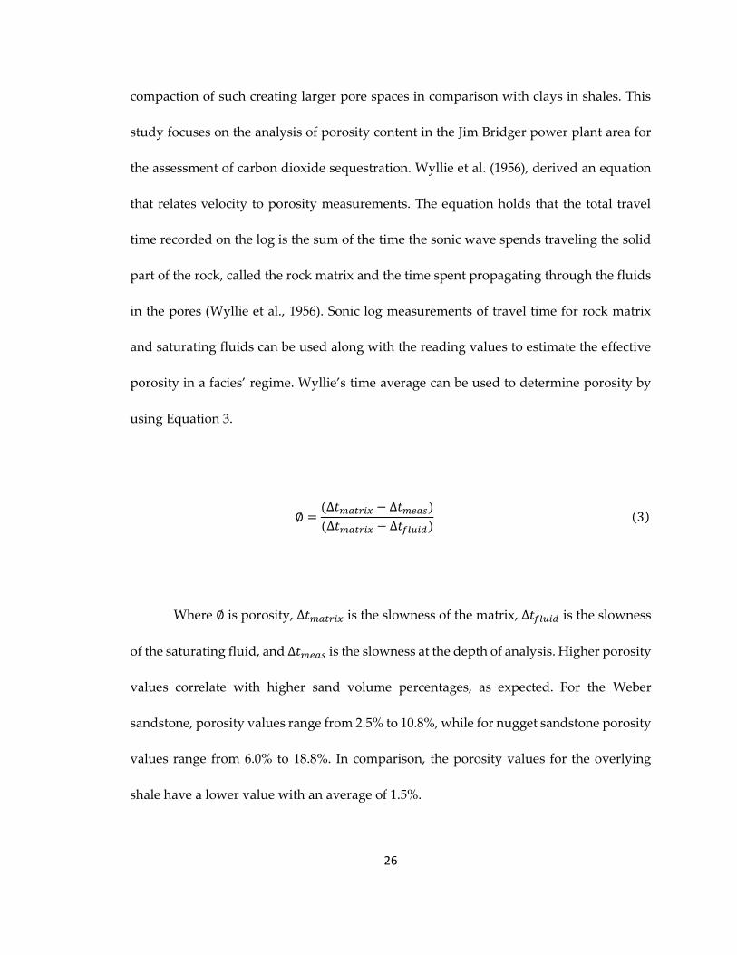
compaction of such creating larger pore spaces in comparison with clays in shales. This
study focuses on the analysis of porosity content in the Jim Bridger power plant area for
the assessment of carbon dioxide sequestration. Wyllie et al. (1956), derived an equation
that relates velocity to porosity measurements. The equation holds that the total travel
time recorded on the log is the sum of the time the sonic wave spends traveling the solid
part of the rock, called the rock matrix and the time spent propagating through the fluids
in the pores (Wyllie et al., 1956). Sonic log measurements of travel time for rock matrix
and saturating fluids can be used along with the reading values to estimate the effective
porosity in a facies’ regime. Wyllie’s time average can be used to determine porosity by
using Equation 3.
∅ =(∆𝑡𝑚𝑎𝑡𝑟𝑖𝑥 − ∆𝑡𝑚𝑒𝑎𝑠)
(∆𝑡𝑚𝑎𝑡𝑟𝑖𝑥 − ∆𝑡𝑓𝑙𝑢𝑖𝑑) (3)
Where ∅ is porosity, ∆𝑡𝑚𝑎𝑡𝑟𝑖𝑥 is the slowness of the matrix, ∆𝑡𝑓𝑙𝑢𝑖𝑑 is the slowness
of the saturating fluid, and ∆𝑡𝑚𝑒𝑎𝑠 is the slowness at the depth of analysis. Higher porosity
values correlate with higher sand volume percentages, as expected. For the Weber
sandstone, porosity values range from 2.5% to 10.8%, while for nugget sandstone porosity
values range from 6.0% to 18.8%. In comparison, the porosity values for the overlying
shale have a lower value with an average of 1.5%.
27
2.1.4 Shear modulus and lame constant
Elastic attributes calculated from measured logs often provide additional
quantitative analysis for a reservoir. Relationships previously described in this chapter
are useful for determining the characteristic of specific lithology and facies. While such
information is of utmost value in the reservoir, seismic signatures influenced by fluid
saturation and rock properties must be differentiated. (lame constant) and (shear
modulus) can be used as a lithology and fluid discriminator by translating P impedance
and S impedance values into rigidity and incompressibility. Equation 4 and 5 are used for
the calculations of and .
𝜆𝜌 = 𝐼2𝑝 − 2𝐼2
𝑠 (4)
𝜇𝜌 = 𝐼2𝑠 (5)
Where 𝜆 is the lame constant, 𝜇 is the shear modulus, 𝐼𝑝 is the P-wave impedance,
𝐼𝑠 is the S-wave impedance, and 𝜌 is the density. Cross plot analysis of and can aid
in the discrimination of lithology and fluid (Goodway et al., 1997). Figure 2.1 demonstrate
typical values of the attributes for different lithologic and fluid compositions. Values
observed at the well location range from 13.1 units to 29.2 units for normalized and
from 28.8 units to 49.0 units for normalized at the sand-rich intervals. A cross-plot of
such values indicate a porous rich sandstone. Figure 2.2 displays the cross-plot of and
at the RSU-#1 well location.
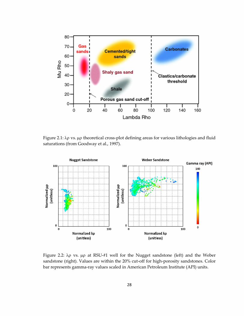
28
Figure 2.1: vs. theoretical cross-plot defining areas for various lithologies and fluid
saturations (from Goodway et al., 1997).
Figure 2.2: vs. at RSU-#1 well for the Nugget sandstone (left) and the Weber
sandstone (right). Values are within the 20% cut-off for high-porosity sandstones. Color
bar represents gamma-ray values scaled in American Petroleum Institute (API) units.
29
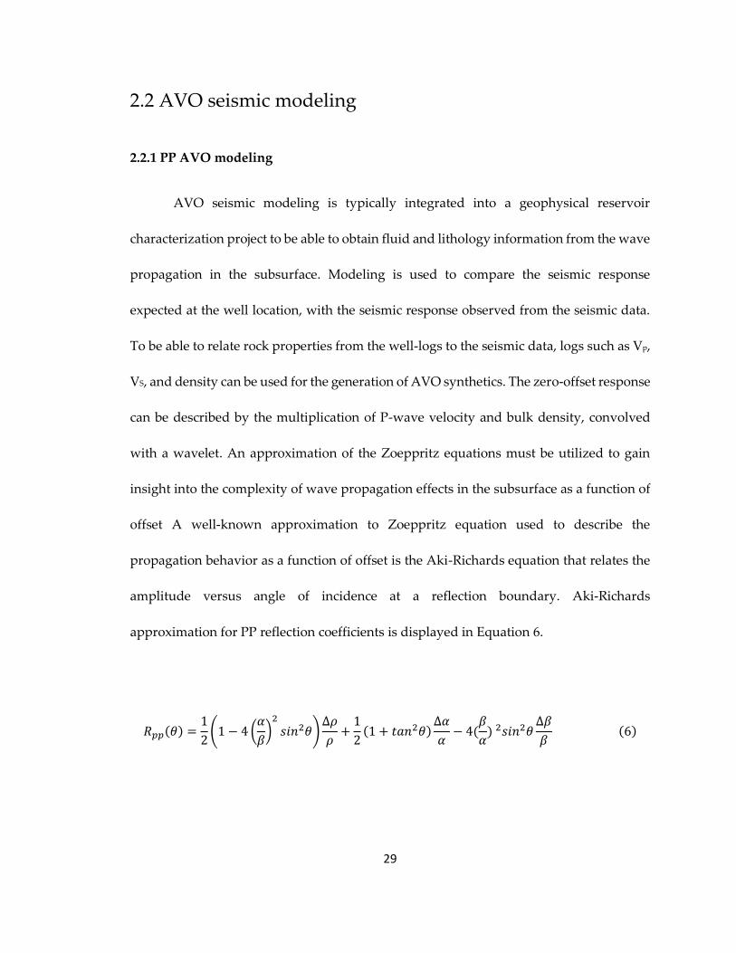
2.2 AVO seismic modeling
2.2.1 PP AVO modeling
AVO seismic modeling is typically integrated into a geophysical reservoir
characterization project to be able to obtain fluid and lithology information from the wave
propagation in the subsurface. Modeling is used to compare the seismic response
expected at the well location, with the seismic response observed from the seismic data.
To be able to relate rock properties from the well-logs to the seismic data, logs such as Vp,
VS, and density can be used for the generation of AVO synthetics. The zero-offset response
can be described by the multiplication of P-wave velocity and bulk density, convolved
with a wavelet. An approximation of the Zoeppritz equations must be utilized to gain
insight into the complexity of wave propagation effects in the subsurface as a function of
offset A well-known approximation to Zoeppritz equation used to describe the
propagation behavior as a function of offset is the Aki-Richards equation that relates the
amplitude versus angle of incidence at a reflection boundary. Aki-Richards
approximation for PP reflection coefficients is displayed in Equation 6.
𝑅𝑝𝑝(𝜃) =1
2(1 − 4 (
𝛼
𝛽)
2
𝑠𝑖𝑛2𝜃)∆𝜌
𝜌+
1
2(1 + 𝑡𝑎𝑛2𝜃)
∆𝛼
𝛼− 4(
𝛽
𝛼) 2𝑠𝑖𝑛2𝜃
∆𝛽
𝛽 (6)
30
Where 𝑅𝑝𝑝 is the reflection coefficient for PP reflections, 𝜌 is average density, α is
average P-wave velocity, β is average S-wave velocity, and ∆ refers to the change of the
parameter. Finally, 𝜃 refers to the average of the incident and transmitted angles.
Figure 2.3: PP reflection AVO modeling at RSU-#1 well location. The upper target is
defined as the Nugget sandstone, and the lower target is defined as the Weber sandstone.
Figure 2.3 shows the PP reflection AVO model for Nugget and Weber sandstones.
The AVO response indicates a slight increase in amplitude with increasing offset,
suggesting a class 3 AVO response.
31
2.2.2 PS AVO modeling
Converted-wave AVO modeling considers the mode conversion of the
propagating wave from a P-wave to an S-wave at the boundary interface. Figure 1.3
displays a schematic diagram of a P-wave propagating and mode conversion occurring at
the interface. Due to the difference in a wave’s propagation from compressional motion
(P-waves) to shear motion (S-waves), multiple rock properties can be analyzed for each of
them. Fluids have zero rigidity; thus S-waves cannot travel through fluids. In principle,
shear-wave velocities are significantly affected by lithologic properties and are much less
affected by the saturating fluid within the rock matrix. Conversely, compressional
primary waves are both affected by lithology and fluid saturation.
A distinct Zoeppritz approximation must be used, incorporating effects of mode
conversion and S-wave propagation to be able to characterize the converted-wave
amplitudes as a function of offset. Equation 1 displays the PS AVO equations used for
such; thus, the converted-wave response depends only on the contrasts in shear velocity
and density. This is substantially different and simpler than the PP case; where the
response depends upon contrasts in the compressional velocity, shear velocity, and
density (Gray, 2003).
32
Figure 2.4: PS reflection AVO modeling at RSU-#1 well location. The upper target is
defined as the Nugget sandstone, and the lower target is defined as the Weber sandstone.
Figure 2.4 shows the PS reflection AVO model for Nugget and Weber sandstones.
The AVO response indicates small negative amplitudes in the near offsets and
increasingly negative amplitudes in far offsets, suggesting a Class 3 AVO response.
33
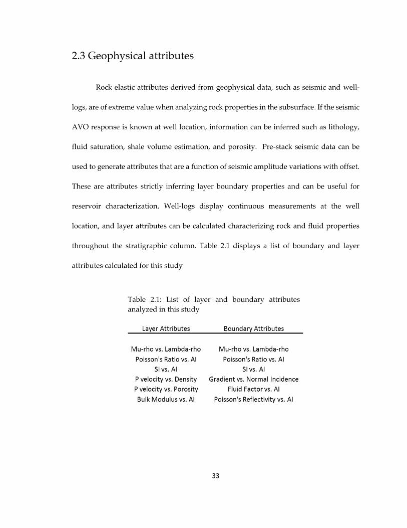
2.3 Geophysical attributes
Rock elastic attributes derived from geophysical data, such as seismic and well-
logs, are of extreme value when analyzing rock properties in the subsurface. If the seismic
AVO response is known at well location, information can be inferred such as lithology,
fluid saturation, shale volume estimation, and porosity. Pre-stack seismic data can be
used to generate attributes that are a function of seismic amplitude variations with offset.
These are attributes strictly inferring layer boundary properties and can be useful for
reservoir characterization. Well-logs display continuous measurements at the well
location, and layer attributes can be calculated characterizing rock and fluid properties
throughout the stratigraphic column. Table 2.1 displays a list of boundary and layer
attributes calculated for this study
Table 2.1: List of layer and boundary attributes
analyzed in this study
34
Figure 2.5: Boundary attributes from seismic data. vs. (left) and Normal Incidence
vs. Gradient (left). The color bar represents the number of sample points in the graph.
Figure 2.6: Layer attributes from well-logs. AI vs. (left) and normalized vs. (right).
The color bar represents gamma-ray values.
35
2.4 Sensitivity analysis
2.4.1 Porosity
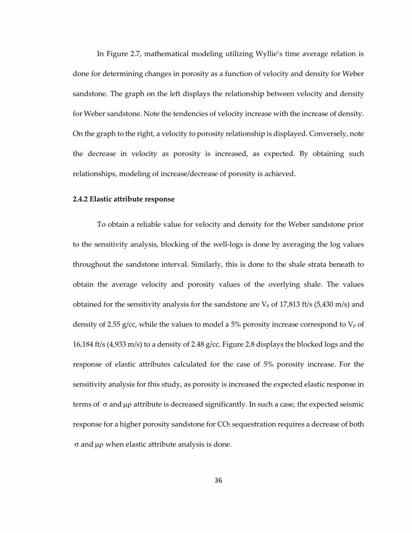
Sensitivities of reflection coefficients to each bulk elastic parameter can be
computed as the partial derivative of the seismic reflectivities relative to each parameter
(Gomez and Tatham, 2005). The sensitivity of reflectivity to porosity variations are
calculated to determine the seismic signature of target sandstones with increased or
decreased porosity for carbon dioxide sequestration purposes. According to Wyllie’s time
average equation (1954), porosity can be calculated as a function of velocity and density.
To be able to characterize the seismic response due to changes in porosity, the variations
in both velocity and density for a specific target sandstone are be calculated. Wyllie’s time
average equation has the form of Equation 4.
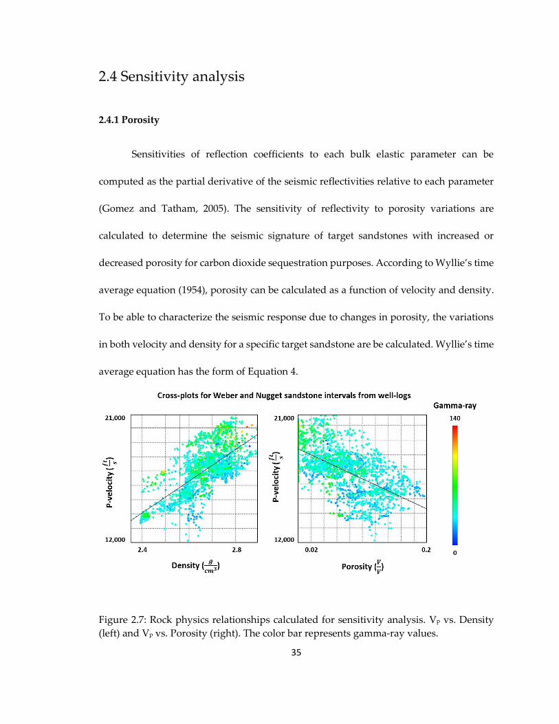
Figure 2.7: Rock physics relationships calculated for sensitivity analysis. Vp vs. Density
(left) and Vp vs. Porosity (right). The color bar represents gamma-ray values.
36
In Figure 2.7, mathematical modeling utilizing Wyllie’s time average relation is
done for determining changes in porosity as a function of velocity and density for Weber
sandstone. The graph on the left displays the relationship between velocity and density
for Weber sandstone. Note the tendencies of velocity increase with the increase of density.
On the graph to the right, a velocity to porosity relationship is displayed. Conversely, note
the decrease in velocity as porosity is increased, as expected. By obtaining such
relationships, modeling of increase/decrease of porosity is achieved.
2.4.2 Elastic attribute response
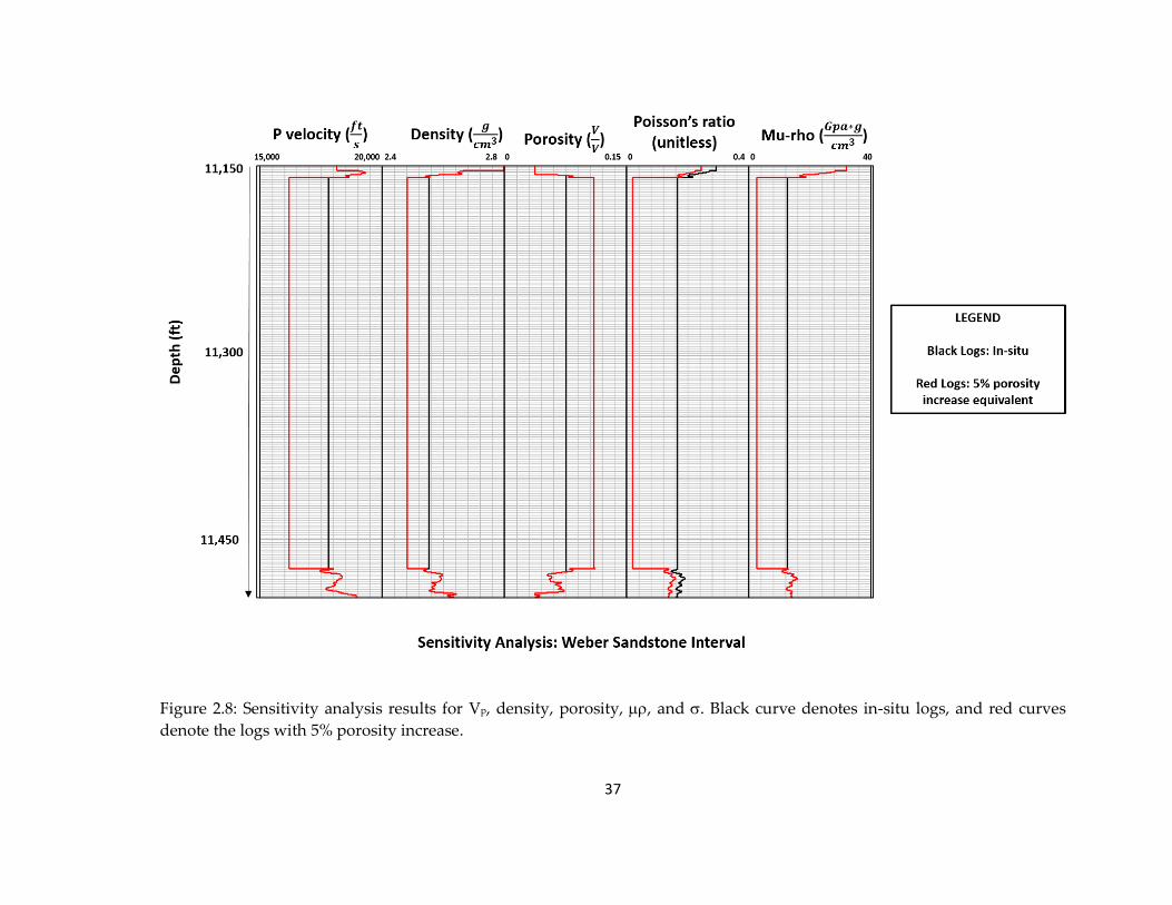
To obtain a reliable value for velocity and density for the Weber sandstone prior
to the sensitivity analysis, blocking of the well-logs is done by averaging the log values
throughout the sandstone interval. Similarly, this is done to the shale strata beneath to
obtain the average velocity and porosity values of the overlying shale. The values
obtained for the sensitivity analysis for the sandstone are Vp of 17,813 ft/s (5,430 m/s) and
density of 2.55 g/cc, while the values to model a 5% porosity increase correspond to Vp of
16,184 ft/s (4,933 m/s) to a density of 2.48 g/cc. Figure 2.8 displays the blocked logs and the
response of elastic attributes calculated for the case of 5% porosity increase. For the
sensitivity analysis for this study, as porosity is increased the expected elastic response in
terms of and attribute is decreased significantly. In such a case, the expected seismic
response for a higher porosity sandstone for CO2 sequestration requires a decrease of both
and when elastic attribute analysis is done.
37
Figure 2.8: Sensitivity analysis results for Vp, density, porosity, , and . Black curve denotes in-situ logs, and red curves
denote the logs with 5% porosity increase.
38
Chapter 3
PP reflection seismic processing
Seismic processing of conventional PP seismic data allows for the generation of a
reliable image of the subsurface used in oil and gas prospecting or carbon dioxide
sequestration studies. In this chapter, the time processing workflow for the vertical
geophone acquired seismic data is described. Shot gather data processed by Geokinetics
in 2010 is used as a starting point for Offset Vector Tile (OVT) generation prior to
migration for the preservation of azimuthal amplitude information. Posterior to
conventional time processing, remnant random/coherent noise and small errors in the
velocity model used for NMO may still be present in the data. Generally, conditioning the
gathers after processing is recommended for obtaining a subsurface seismic image that
most accurately represents the actual geology. Gather-conditioning post-processing
sequence utilized includes random/linear noise removal, residual velocity correction,
removal of unwanted coherent energy (i.e. multiples), f-k filtering, and amplitude
normalization. Figure 3.1 displays the time processing sequence while Figure 3.2 shows
post-migration seismic conditioning of vertical geophone seismic data.
39
3.1 PP seismic processing workflow
3.1.1 Time processing workflow
Figure 3.1: Time processing workflow for P-wave reflection seismic data.
40
3.1.2 Gather-conditioning workflow
Figure 3.2: Representation of the seismic gather-conditioning workflow.
41
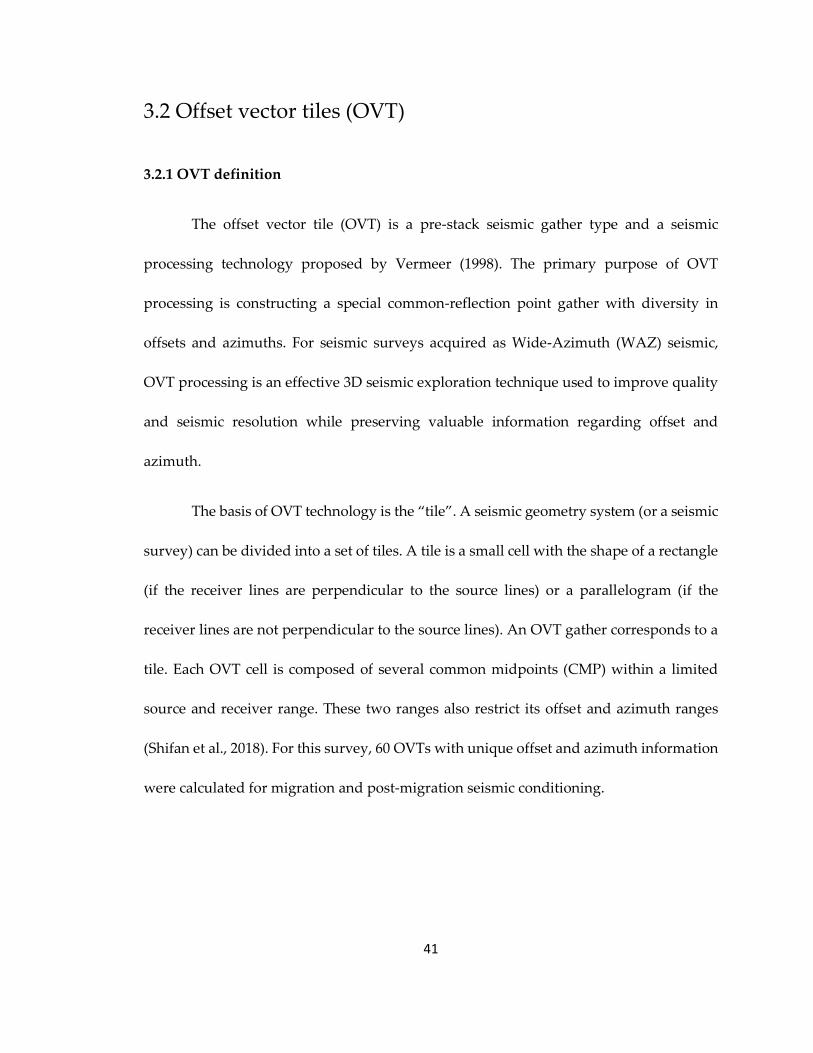
3.2 Offset vector tiles (OVT)
3.2.1 OVT definition
The offset vector tile (OVT) is a pre-stack seismic gather type and a seismic
processing technology proposed by Vermeer (1998). The primary purpose of OVT
processing is constructing a special common-reflection point gather with diversity in
offsets and azimuths. For seismic surveys acquired as Wide-Azimuth (WAZ) seismic,
OVT processing is an effective 3D seismic exploration technique used to improve quality
and seismic resolution while preserving valuable information regarding offset and
azimuth.
The basis of OVT technology is the “tile”. A seismic geometry system (or a seismic
survey) can be divided into a set of tiles. A tile is a small cell with the shape of a rectangle
(if the receiver lines are perpendicular to the source lines) or a parallelogram (if the
receiver lines are not perpendicular to the source lines). An OVT gather corresponds to a
tile. Each OVT cell is composed of several common midpoints (CMP) within a limited
source and receiver range. These two ranges also restrict its offset and azimuth ranges
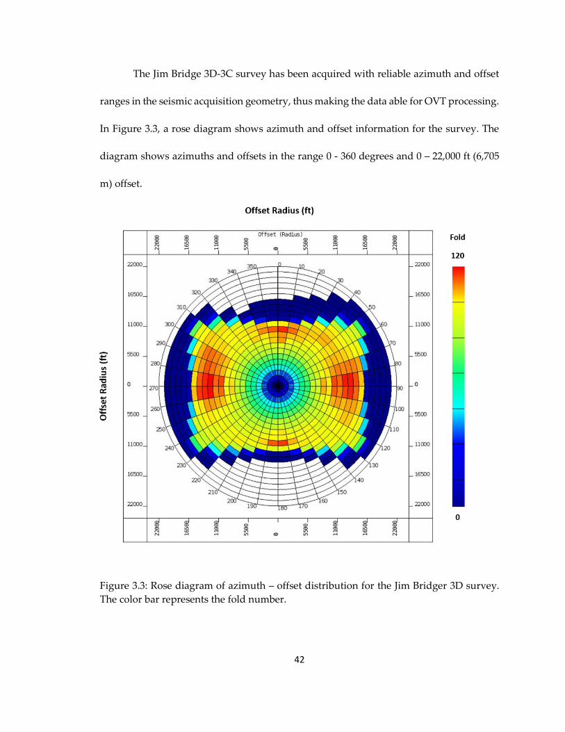
(Shifan et al., 2018). For this survey, 60 OVTs with unique offset and azimuth information
were calculated for migration and post-migration seismic conditioning.
42
The Jim Bridge 3D-3C survey has been acquired with reliable azimuth and offset
ranges in the seismic acquisition geometry, thus making the data able for OVT processing.
In Figure 3.3, a rose diagram shows azimuth and offset information for the survey. The
diagram shows azimuths and offsets in the range 0 - 360 degrees and 0 – 22,000 ft (6,705
m) offset.
Figure 3.3: Rose diagram of azimuth – offset distribution for the Jim Bridger 3D survey.
The color bar represents the fold number.

43
Figure 3.4: Offset vector tiles (OVT) theoretical distribution. The color bar represents the
ring number.
Figure 3.4 displays a diagram for the assignment of each offset vector tile. Each tile
corresponds to a unique azimuth – offset range and traces may be placed within each of
these distinct bins. Only the reciprocal tiles are used to increase the number of traces
within each bin. That is, azimuth values ranging from 0 – 180 degrees are used to avoid
redundant azimuthal information. Furthermore, to maximize fold the data can be sorted
in OVT sectors where a range of tiles are utilized for a larger azimuthal range such as
encompassing bins within 15-degree sectors. After offset vector tiles area assigned, the
CDP gathers can be sorted in terms of offset and azimuth to observe the changes in

44
velocity with respect to offset, and azimuth corresponding to anisotropy for primary
reflectors, such as CDP gathers in Figure 3.5.
Figure 3.5: CDP gathers sorted as common offset and common azimuth to demonstrate
the effect of azimuthal velocity variations. COCA values range from 1,000 to 13,000 for
each CDP gather.
45
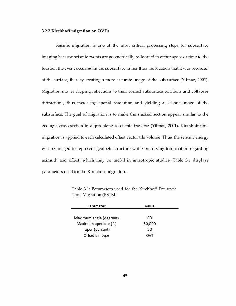
3.2.2 Kirchhoff migration on OVTs
Seismic migration is one of the most critical processing steps for subsurface
imaging because seismic events are geometrically re-located in either space or time to the
location the event occurred in the subsurface rather than the location that it was recorded
at the surface, thereby creating a more accurate image of the subsurface (Yilmaz, 2001).
Migration moves dipping reflections to their correct subsurface positions and collapses
diffractions, thus increasing spatial resolution and yielding a seismic image of the
subsurface. The goal of migration is to make the stacked section appear similar to the
geologic cross-section in depth along a seismic traverse (Yilmaz, 2001). Kirchhoff time
migration is applied to each calculated offset vector tile volume. Thus, the seismic energy
will be imaged to represent geologic structure while preserving information regarding
azimuth and offset, which may be useful in anisotropic studies. Table 3.1 displays
parameters used for the Kirchhoff migration.
Table 3.1: Parameters used for the Kirchhoff Pre-stack
Time Migration (PSTM)
46
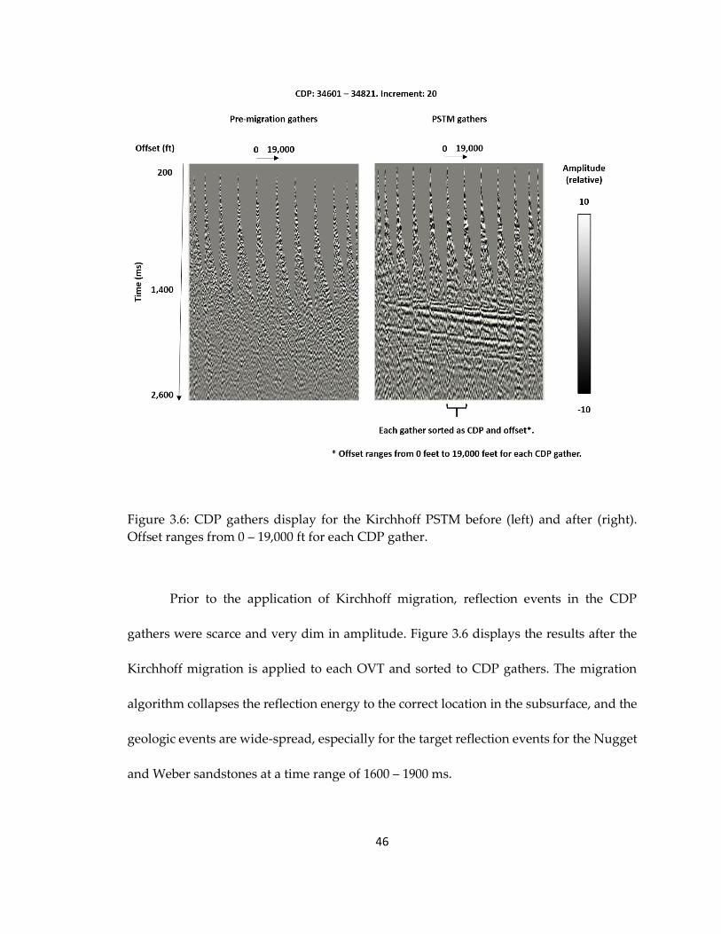
Figure 3.6: CDP gathers display for the Kirchhoff PSTM before (left) and after (right).
Offset ranges from 0 – 19,000 ft for each CDP gather.
Prior to the application of Kirchhoff migration, reflection events in the CDP
gathers were scarce and very dim in amplitude. Figure 3.6 displays the results after the
Kirchhoff migration is applied to each OVT and sorted to CDP gathers. The migration
algorithm collapses the reflection energy to the correct location in the subsurface, and the
geologic events are wide-spread, especially for the target reflection events for the Nugget
and Weber sandstones at a time range of 1600 – 1900 ms.
47
3.3 Gather-conditioning
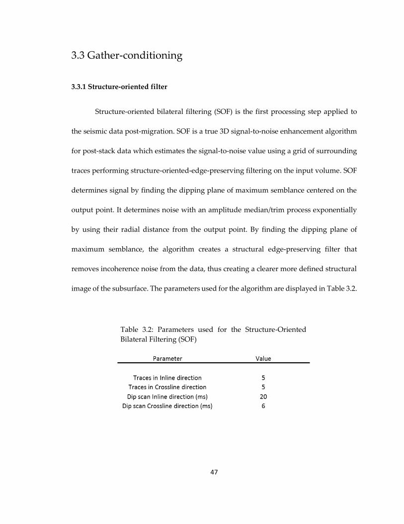
3.3.1 Structure-oriented filter
Structure-oriented bilateral filtering (SOF) is the first processing step applied to
the seismic data post-migration. SOF is a true 3D signal-to-noise enhancement algorithm
for post-stack data which estimates the signal-to-noise value using a grid of surrounding
traces performing structure-oriented-edge-preserving filtering on the input volume. SOF
determines signal by finding the dipping plane of maximum semblance centered on the
output point. It determines noise with an amplitude median/trim process exponentially
by using their radial distance from the output point. By finding the dipping plane of
maximum semblance, the algorithm creates a structural edge-preserving filter that
removes incoherence noise from the data, thus creating a clearer more defined structural
image of the subsurface. The parameters used for the algorithm are displayed in Table 3.2.
Table 3.2: Parameters used for the Structure-Oriented
Bilateral Filtering (SOF)
48
Figure 3.7: CDP gathers display for Structure-Oriented Filtering (SOF) before (left), after
(middle), and difference (right). Offset ranges from 0 – 19,000 ft for each CDP gather.
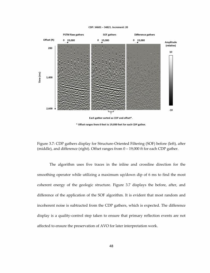
The algorithm uses five traces in the inline and crossline direction for the
smoothing operator while utilizing a maximum up/down dip of 6 ms to find the most
coherent energy of the geologic structure. Figure 3.7 displays the before, after, and
difference of the application of the SOF algorithm. It is evident that most random and
incoherent noise is subtracted from the CDP gathers, which is expected. The difference
display is a quality-control step taken to ensure that primary reflection events are not
affected to ensure the preservation of AVO for later interpretation work.
49
3.3.2 VTI and HTI corrections
Vertical Transverse Isotropy (VTI) and Horizontal Transverse isotropy (HTI)
induce changes in the propagating velocity of the waveform depending on the direction
of travel. Such changes in anisotropy within the survey will create varying velocities
required to flatten the reflection events on CDP gathers within the seismic volume.
Anisotropic velocity variations due to VTI and HTI must be accounted for proper imaging
of the geologic structure.
The VTI correction algorithm calculates the variations of velocity from Normal
Incidence (NI) and Poisson’s Reflectivity (PR) on a CDP gather. The algorithm by Swan
(2001) describes the method for computing the residual velocity corrections based on AVO
attributes for flattening the gathers. The technique typically corrects a 2% error in the RMS
field. If the error is larger than 2%, then this method can be used in iterations (Swan, 2001).
The algorithm outputs a volume of velocity changes which are then smoothed and added
to the original velocity field. The initial velocity field is removed for NMO correction, and
the new one is applied.
Azimuthal anisotropy, also known as HTI, produces a pattern of slowness versus
azimuth which is elliptical. For azimuthal anisotropy corrections, the algorithm
decomposes arrival time “errors” caused by anisotropy into parameters estimating the
elliptical anisotropy and uses least-squares fitting to determine the parameters which best
define the anisotropic ellipse.
50
Figure 3.8: CDP gathers display for VTI/HTI velocity correction before (left) and after
(right). Offset ranges from 0 – 19,000 ft for each CDP gather.
Table 3.3 shows the parameters used for the VTI and HTI corrections. For the VTI
algorithm, a maximum of 12% change in velocity can be calculated for seismic energy with
a central frequency of 35 Hz. A running window of 48 ms is used for the statistics
Table 3.3: Parameters used for the VTI and HTI velocity corrections
51
calculations. The stack response is expected to improve significantly after applying
corrections for vertical and horizontal anisotropy because the velocity errors from
azimuthal variations are minimized and flattening of the gathers is expected. The stack
should have increased focusing of events by increasing the amplitude for each CDP
location while improving the reliability of the AVO response displayed in the stack.
Figure 3.8 displays the CDP gathers before and after the anisotropic correction. It is
evident the primary reflection events are flatter after the anisotropic corrections. Figure
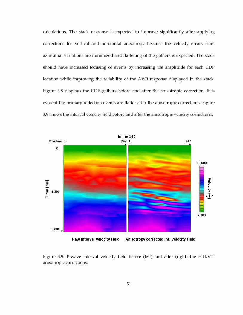
3.9 shows the interval velocity field before and after the anisotropic velocity corrections.
Figure 3.9: P-wave interval velocity field before (left) and after (right) the HTI/VTI
anisotropic corrections.
52
3.3.3 Radon de-multiple
Multiples and converted-waves are coherent periodic noise in the seismic data
with move-out that may destructively or constructively interfere with the primary
reflections of interest. The geologic structure and amplitude-versus-offset (AVO)
characteristics may be affected by such types of unwanted coherent signal. Such wave
phenomena are required to be removed, so as not to be detrimental to the primary
reflection signal to image the geologic structure reliably. A high-resolution Radon
algorithm is used for the removal of multiples, converted-waves, and any unwanted
signal from the data. Radon utilizes the coherent signal from the data and transforms the
data from the space-time domain to the - domain. In such a domain, the dipping
hyperbolic events, such as multiples, in space-time domain will be defined as a “point”
with a high numbered p (move-out) in the - domain (Russell et al., 1990). By modeling
the primary energy in this domain, the parabolic events with move-out in a CDP gather
can be muted, and only the values of p (move-out) that correspond to zero, or close to
zero, are kept (Russell et al., 1990).
Either linear or parabolic moveout can be modeled with the Radon transform.
When the linear method is selected, the high-resolution method is used throughout the
transform domain. The generalized least-squares method is used to minimize the
differences between the input data and the computed model data. The advantage of doing
this is that the wavelet shape and amplitude of primaries and multiples are accurately
obtained, and multiples can be removed by simple subtraction without the need for
53
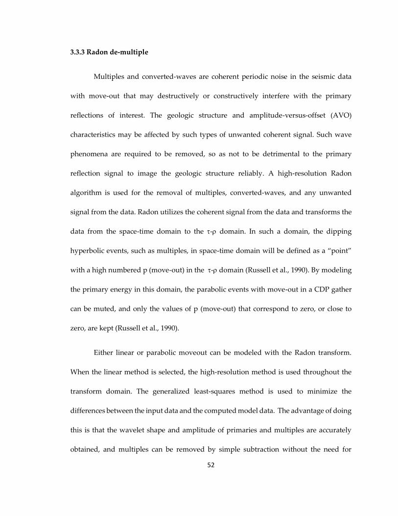
adaptive subtraction techniques. The limitation with conventional Radon is that some
energy from some events can appear in the “wrong place” in the transform domain due
to aliasing. Radon addresses this problem by predicting where the main events lie in the
transform domain, emphasizing these areas and suppressing other regions. This
emphasis and suppression are done via a set of weights that vary with move out.
Table 3.4 shows the parameters used for the calculation of the tau-p transform and
the polygon mute applied for the removal of multiple events. The reference offset for the
estimate of the move-out in milliseconds is 19,800 ft (6,035 m) while the minimum and
maximum RNMO are -300 ms and 650 ms, respectively. The - transform works in the
frequency range of 7 – 100 Hz and only on CDP gathers with a minimum of eight traces
for accurate modeling of multiple events. The p (move-out) ramp is chosen to be of 80 ms.
The polygon mute is designed to mute most of the multiple near the target area at 2,000
Table 3.4: Parameters (right) and polygon mute (left) in - domain for Radon de-
multiple
54
ms with a mute value of 60 ms while allowing more energy to pass in the shallow area as
it is not affected by multiples as much.
Figure 3.10: CDP gathers display for Radon de-multiple before (left), after (middle), and
difference (right). Offset ranges from 0 – 19,000 ft for each CDP gather.
Figure 3.10 shows CDP gathers before, after, and the difference from the
application of Radon de-multiple. The primary reflection events should be unaltered after
the application of the algorithm and only coherent energy with a move-out should be
removed from the CDP gathers.
55
3.3.4 CDP domain noise attenuation
Remnant linear coherent and incoherent noise may still be present in the data,
which may have to be removed for the imaging of the subsurface. Linear noise attenuation
and a - domain noise attenuation method are used on CDP gathers for removal of such
coherent and incoherent noise.
The linear noise present in the data is removed utilizing a frequency-wavenumber
(f-k) filter by transforming the data into the f-k domain and applying a mute to the data
not corresponding to primary flat reflections. This module attenuates events with slopes
(up and down) smaller than the corresponding slope of the specified input velocity. The
process works by transforming an ensemble of seismic shot data from the time-space
domain to spatial frequency domain. Each frequency is convolved with a select weighting
function, which is formed from the array of the signals with the desired frequency band.
Velocities up to 12,000 ft/s (3,658 m/s) are attenuated by developing a filter in the f-k
domain to remove such data with the corresponding velocity.
A technique is used utilizing the Radon transform for removal of incoherent and
random energy in the CDP gather. The primary events are modeled in the - domain
using a high-resolution Radon transform (refer to section 3.3.3). The primary-only model
is output from the algorithm and scaled down to 66.667%, while the input dataset is scaled
down to 33.333% and the result is obtained by addition of both the input and primary-
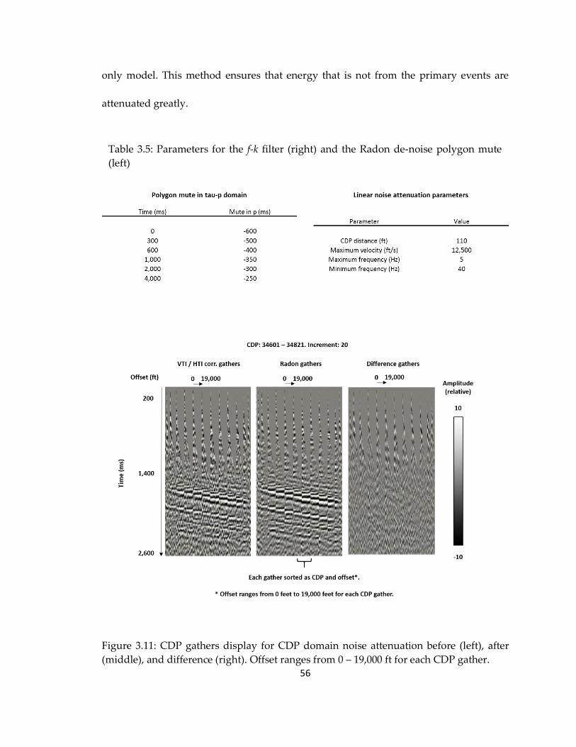
56
only model. This method ensures that energy that is not from the primary events are
attenuated greatly.
Figure 3.11: CDP gathers display for CDP domain noise attenuation before (left), after
(middle), and difference (right). Offset ranges from 0 – 19,000 ft for each CDP gather.
Table 3.5: Parameters for the f-k filter (right) and the Radon de-noise polygon mute
(left)
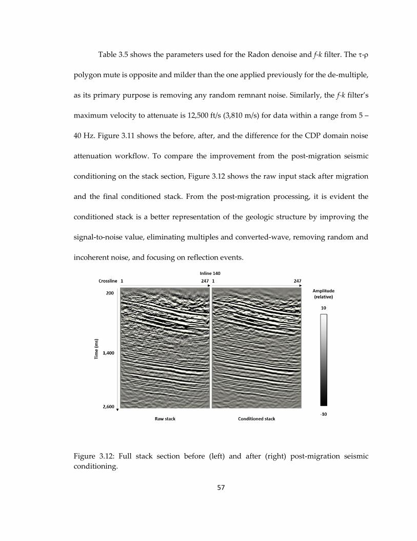
57
Table 3.5 shows the parameters used for the Radon denoise and f-k filter. The -
polygon mute is opposite and milder than the one applied previously for the de-multiple,
as its primary purpose is removing any random remnant noise. Similarly, the f-k filter’s
maximum velocity to attenuate is 12,500 ft/s (3,810 m/s) for data within a range from 5 –
40 Hz. Figure 3.11 shows the before, after, and the difference for the CDP domain noise
attenuation workflow. To compare the improvement from the post-migration seismic
conditioning on the stack section, Figure 3.12 shows the raw input stack after migration
and the final conditioned stack. From the post-migration processing, it is evident the
conditioned stack is a better representation of the geologic structure by improving the
signal-to-noise value, eliminating multiples and converted-wave, removing random and
incoherent noise, and focusing on reflection events.
Figure 3.12: Full stack section before (left) and after (right) post-migration seismic
conditioning.
58
Chapter 4
AVO simultaneous inversion
IFP’s (Institut Francais du Petrole) pre-stack AVO simultaneous three-term
inversion algorithm is a Bayesian non-linear data fitting method with an objective of
extracting accurate information of the subsurface elastic and petrophysical properties
from the seismic data. A prediction of properties can be calculated by solving the Aki-
Richards AVO equation using an initial model of the subsurface along with the seismic
data. In an iterative process, the model is updated to minimize the error or misfit of the
predicted data from a background model and observed data (seismic). Various iterations
are completed until the misfit is reduced sufficiently. During inversion, geological
knowledge, pre-stack seismic amplitude, and well-log information are combined to build
optimal elastic parameter distributions, which is consistent with all input data. IFP Pre-
stack inversion is based on a Bayesian formalism, in which the seismic noise and the elastic
model uncertainties are assumed to be described by Gaussian probabilities having zero
mean, with a covariance operator in the data space and the model space. The algorithm
has been developed by IFP and integrated into Paradigm Geophysical Software.
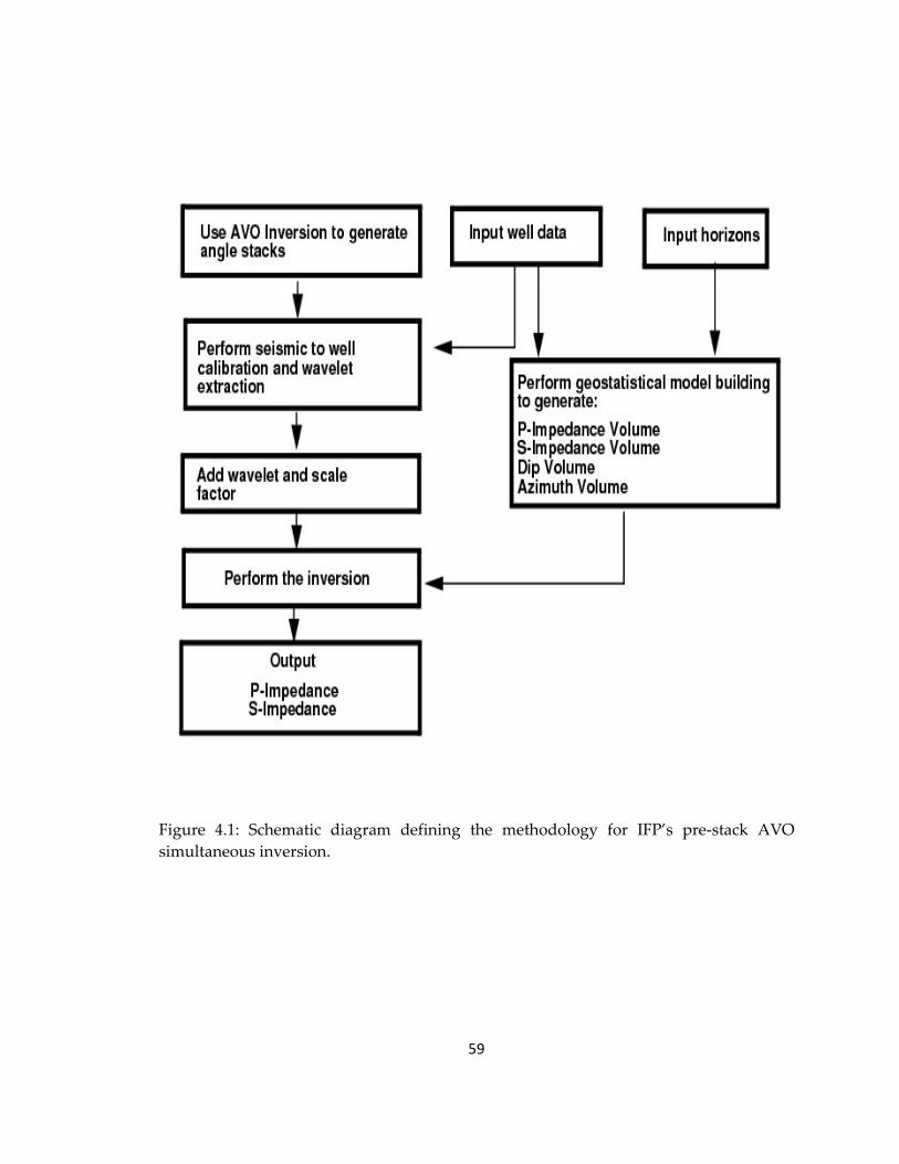
59
Figure 4.1: Schematic diagram defining the methodology for IFP’s pre-stack AVO
simultaneous inversion.
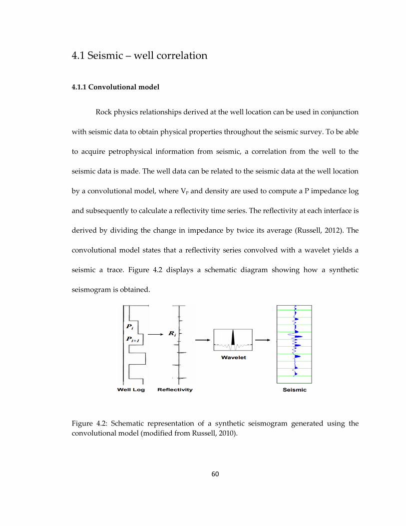
60
4.1 Seismic – well correlation
4.1.1 Convolutional model
Rock physics relationships derived at the well location can be used in conjunction
with seismic data to obtain physical properties throughout the seismic survey. To be able
to acquire petrophysical information from seismic, a correlation from the well to the
seismic data is made. The well data can be related to the seismic data at the well location
by a convolutional model, where Vp and density are used to compute a P impedance log
and subsequently to calculate a reflectivity time series. The reflectivity at each interface is
derived by dividing the change in impedance by twice its average (Russell, 2012). The
convolutional model states that a reflectivity series convolved with a wavelet yields a
seismic a trace. Figure 4.2 displays a schematic diagram showing how a synthetic
seismogram is obtained.
Figure 4.2: Schematic representation of a synthetic seismogram generated using the
convolutional model (modified from Russell, 2010).
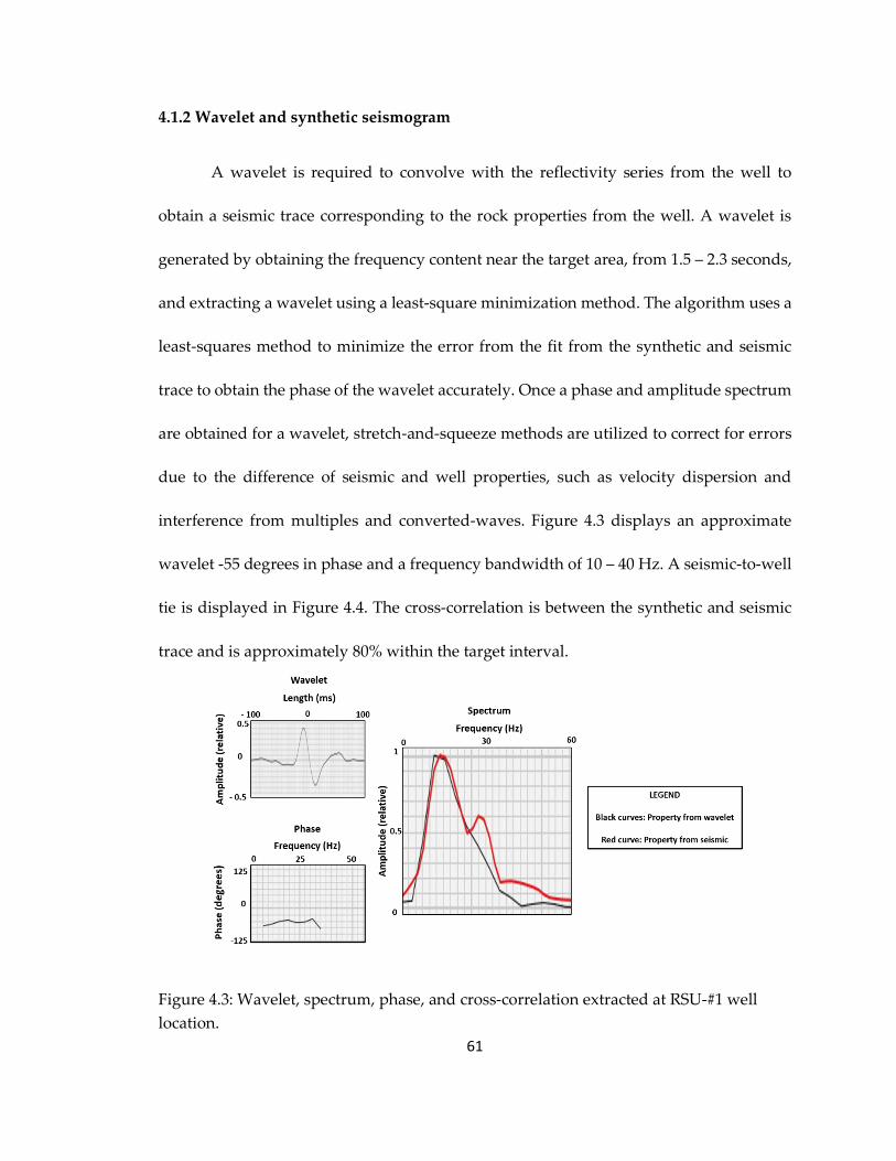
61
4.1.2 Wavelet and synthetic seismogram
A wavelet is required to convolve with the reflectivity series from the well to
obtain a seismic trace corresponding to the rock properties from the well. A wavelet is
generated by obtaining the frequency content near the target area, from 1.5 – 2.3 seconds,
and extracting a wavelet using a least-square minimization method. The algorithm uses a
least-squares method to minimize the error from the fit from the synthetic and seismic
trace to obtain the phase of the wavelet accurately. Once a phase and amplitude spectrum
are obtained for a wavelet, stretch-and-squeeze methods are utilized to correct for errors
due to the difference of seismic and well properties, such as velocity dispersion and
interference from multiples and converted-waves. Figure 4.3 displays an approximate
wavelet -55 degrees in phase and a frequency bandwidth of 10 – 40 Hz. A seismic-to-well
tie is displayed in Figure 4.4. The cross-correlation is between the synthetic and seismic
trace and is approximately 80% within the target interval.
Figure 4.3: Wavelet, spectrum, phase, and cross-correlation extracted at RSU-#1 well
location.
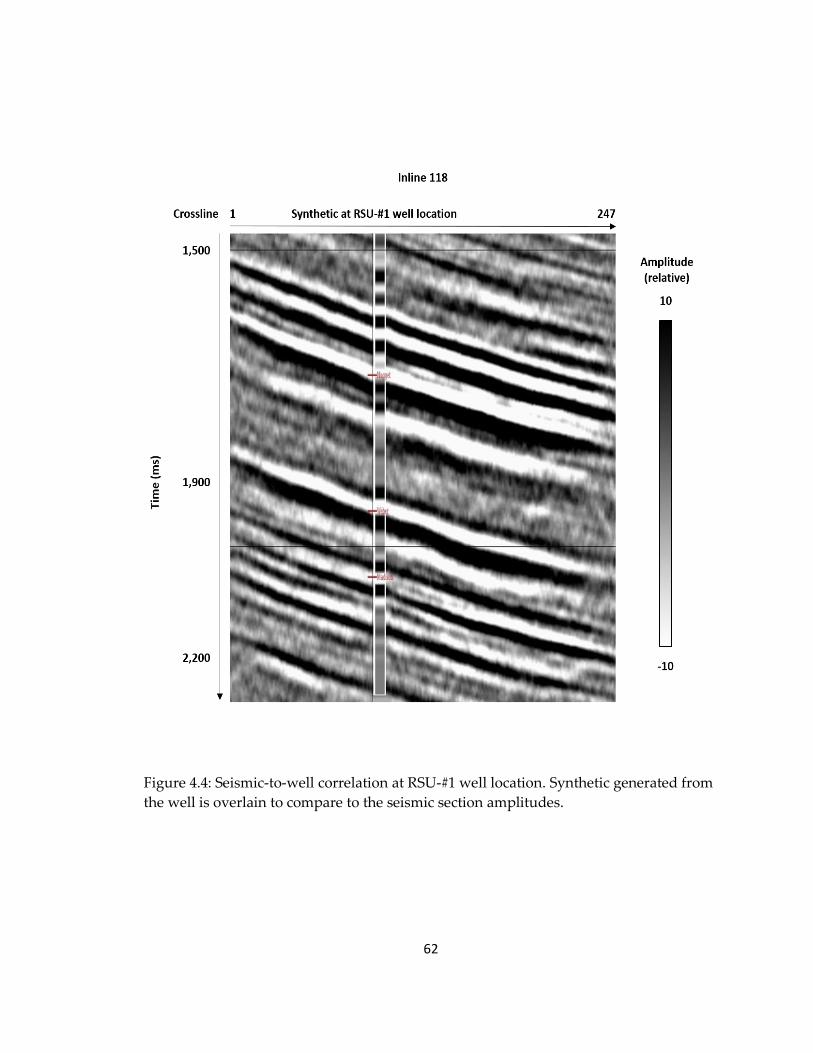
62
Figure 4.4: Seismic-to-well correlation at RSU-#1 well location. Synthetic generated from
the well is overlain to compare to the seismic section amplitudes.
63
4.2 Angle stack generation
4.2.1 Angle rage analysis
The Aki-Richards AVO equations relate the incidence angle of the wave
propagation to reflection amplitude in terms of Vp, Vs, and density. Pre-stack
simultaneous AVO inversion utilizes information from the seismic data within various
incident angle ranges to obtain a solution to the AVO equation and obtain the elastic
properties of interest (P impedance, S impedance, and density). The pre-stack seismic data
is analyzed for incident angle information to generate angle stacks which are input for the
AVO inversion. Ray-tracing techniques are used for calculating the path of waves
propagating through the subsurface that have different propagation velocities, absorption
characteristics, and reflecting surfaces to calculate incident angle information from CDP
gathers (Rawlinson et al., 2007).
Figure 4.5 displays an overlay of angle ranges with the CDP gathers for angle
range analysis. The seismic data is analyzed for each angle range to determine the angle
stacks that display similar signal-to-noise values, coherent amplitude energy, and
attenuation absorption characteristics. Angle ranges utilized for the generation of angle
stacks are 00 – 13 degrees, 08 – 22 degrees, 18 – 32 degrees, and 28 – 42 degrees. Angle
range overlap is desired to maximize the amount of angle information per each angle
range. Such angle ranges display information from the near, middle, and far angles from
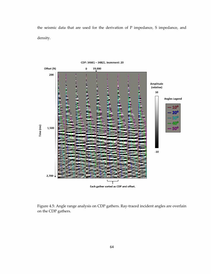
64
the seismic data that are used for the derivation of P impedance, S impedance, and
density.
Figure 4.5: Angle range analysis on CDP gathers. Ray-traced incident angles are overlain
on the CDP gathers.
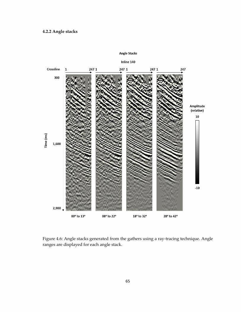
65
4.2.2 Angle stacks
Figure 4.6: Angle stacks generated from the gathers using a ray-tracing technique. Angle
ranges are displayed for each angle stack.
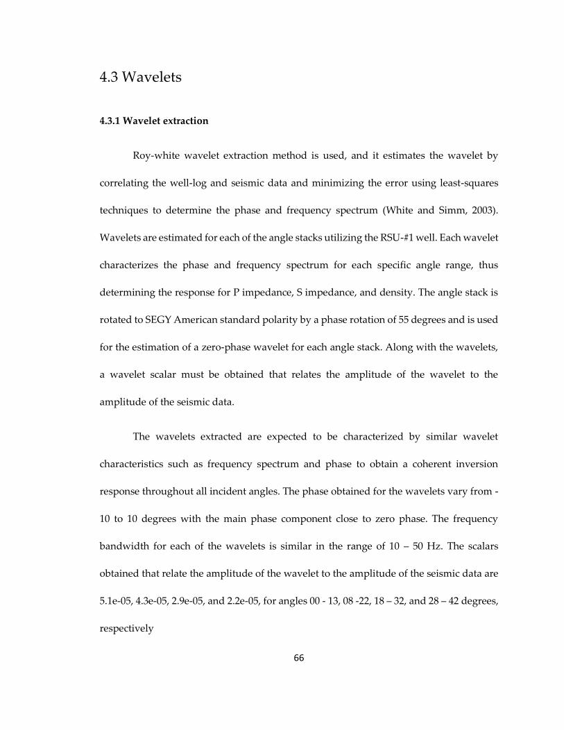
66
4.3 Wavelets
4.3.1 Wavelet extraction
Roy-white wavelet extraction method is used, and it estimates the wavelet by
correlating the well-log and seismic data and minimizing the error using least-squares
techniques to determine the phase and frequency spectrum (White and Simm, 2003).
Wavelets are estimated for each of the angle stacks utilizing the RSU-#1 well. Each wavelet
characterizes the phase and frequency spectrum for each specific angle range, thus
determining the response for P impedance, S impedance, and density. The angle stack is
rotated to SEGY American standard polarity by a phase rotation of 55 degrees and is used
for the estimation of a zero-phase wavelet for each angle stack. Along with the wavelets,
a wavelet scalar must be obtained that relates the amplitude of the wavelet to the
amplitude of the seismic data.
The wavelets extracted are expected to be characterized by similar wavelet
characteristics such as frequency spectrum and phase to obtain a coherent inversion
response throughout all incident angles. The phase obtained for the wavelets vary from -
10 to 10 degrees with the main phase component close to zero phase. The frequency
bandwidth for each of the wavelets is similar in the range of 10 – 50 Hz. The scalars
obtained that relate the amplitude of the wavelet to the amplitude of the seismic data are
5.1e-05, 4.3e-05, 2.9e-05, and 2.2e-05, for angles 00 - 13, 08 -22, 18 – 32, and 28 – 42 degrees,
respectively
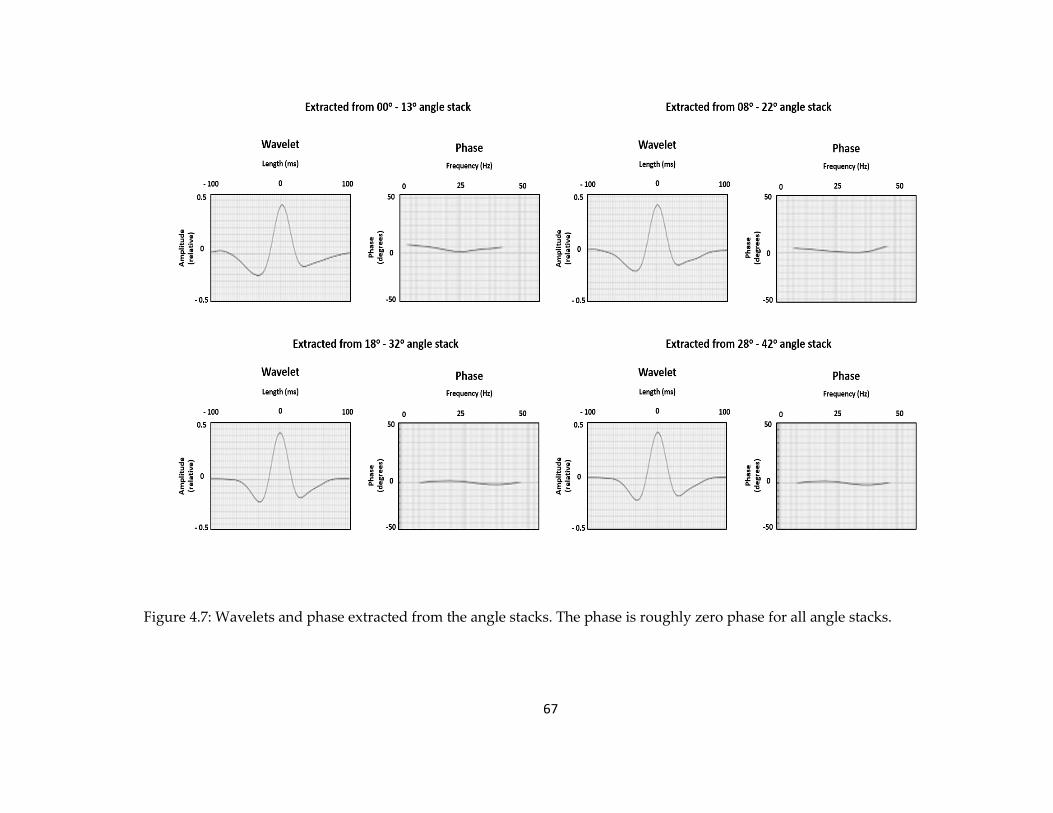
67
Figure 4.7: Wavelets and phase extracted from the angle stacks. The phase is roughly zero phase for all angle stacks.

68
4.4 Low-frequency background model generation
4.4.1 Collocated cokriging of well-logs
Kriging and cokriging are geostatistical techniques used for interpolation
(mapping and contouring) purposes. Both methods are generalized forms of univariate
and multivariate linear regression models, for estimation at a point, over an area, or within
a volume (Chambers et al., 2000). They are linear-weighted averaging methods, similar to
other interpolation methods; however, their weights depend not only on distance but also
on the direction and orientation of the neighboring data to the unsampled location
(Chambers et al., 2000).
Traditional regression methods only use data available at the target location and
fail to use existing spatial correlations from secondary-data control points and the primary
attribute to be estimated. Cokriging methods are used to take advantage of the covariance
between two or more regionalized variables that are related and are appropriate when the
primary attribute of interest (well data) is sparse, but related secondary information
(seismic) is abundant. Geostatistical-data-integration methods yield more-reliable
reservoir models because they capitalize on the strengths of both data types (Journel,
1989).
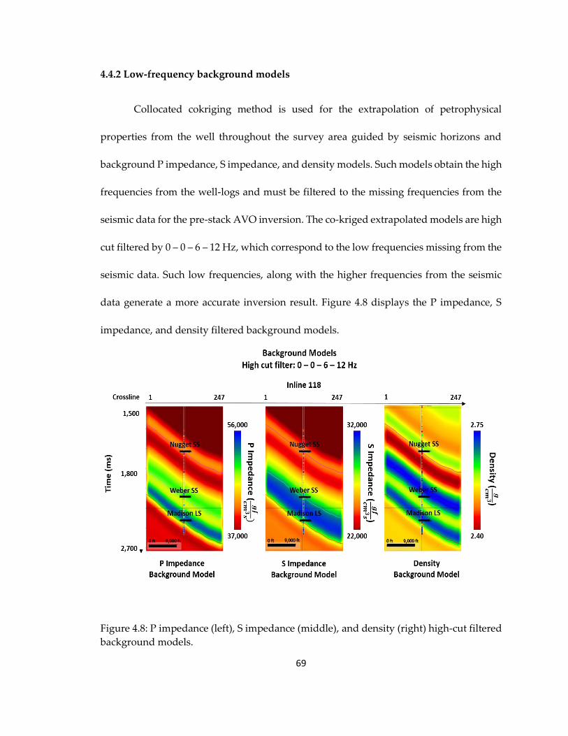
69
4.4.2 Low-frequency background models
Collocated cokriging method is used for the extrapolation of petrophysical
properties from the well throughout the survey area guided by seismic horizons and
background P impedance, S impedance, and density models. Such models obtain the high
frequencies from the well-logs and must be filtered to the missing frequencies from the
seismic data for the pre-stack AVO inversion. The co-kriged extrapolated models are high
cut filtered by 0 – 0 – 6 – 12 Hz, which correspond to the low frequencies missing from the
seismic data. Such low frequencies, along with the higher frequencies from the seismic
data generate a more accurate inversion result. Figure 4.8 displays the P impedance, S
impedance, and density filtered background models.
Figure 4.8: P impedance (left), S impedance (middle), and density (right) high-cut filtered
background models.

70
4.5 AVO Inversion
4.5.1 AVO inversion background
IFP Pre-stack Constrained Stratigraphic Inversion performs simultaneous
inversion of multiple angle stacks to provide P and S impedance volumes and optional
density data. Required for the inversion are two or more angle stacks, a wavelet for each
angle stack, a micro-layer geometry in the form of dip and azimuth volumes, confidence
information for both the seismic data and the background model, a low-frequency
background model, and optional formation volumes. The output from the inversion is P
impedance, S impedance, and density. The inversion can also be used as a standard AI
inversion using one seismic attribute. The IFP Pre-stack Constrained Stratigraphic
Inversion application performs inversion simultaneously for all elastic parameters. The
inversion is a Global 3D and model-based Aki-Richards modeling for consistent estimates
of both P and S impedances.
During the inversion, geological knowledge, pre-stack seismic amplitudes, and
well-log information are combined to build optimal elastic parameter distributions, which
are consistent with all input data.
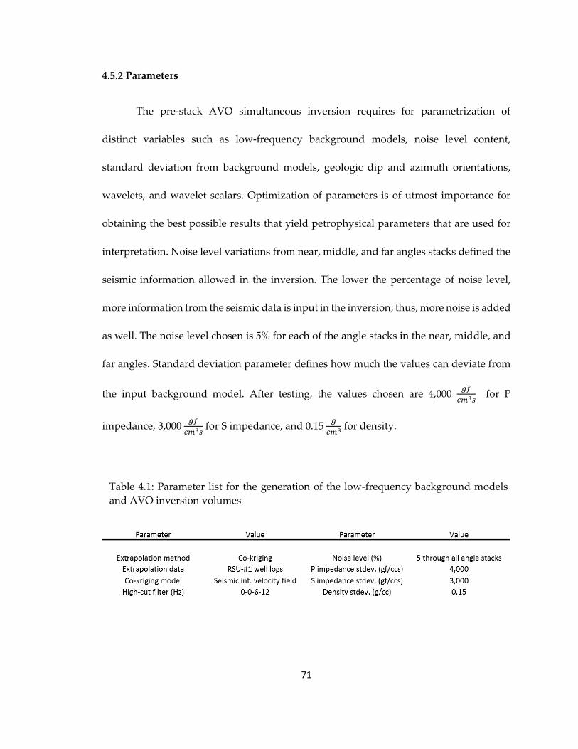
71
4.5.2 Parameters
The pre-stack AVO simultaneous inversion requires for parametrization of
distinct variables such as low-frequency background models, noise level content,
standard deviation from background models, geologic dip and azimuth orientations,
wavelets, and wavelet scalars. Optimization of parameters is of utmost importance for
obtaining the best possible results that yield petrophysical parameters that are used for
interpretation. Noise level variations from near, middle, and far angles stacks defined the
seismic information allowed in the inversion. The lower the percentage of noise level,
more information from the seismic data is input in the inversion; thus, more noise is added
as well. The noise level chosen is 5% for each of the angle stacks in the near, middle, and
far angles. Standard deviation parameter defines how much the values can deviate from
the input background model. After testing, the values chosen are 4,000 𝑔𝑓
𝑐𝑚3𝑠 for P
impedance, 3,000 𝑔𝑓
𝑐𝑚3𝑠 for S impedance, and 0.15
𝑔
𝑐𝑚3 for density.
Table 4.1: Parameter list for the generation of the low-frequency background models
and AVO inversion volumes

72
4.5.2 AVO inversion volumes
The outputs from the AVO inversion algorithm are P impedance, S impedance,
and density volumes. Figure 4.9 displays the volumes obtained from the AVO inversion
with a synthetic overlain respectively. For the P impedance volume, the values range from
25,000 𝑔𝑓
𝑐𝑚3𝑠 and 60,000
𝑔𝑓
𝑐𝑚3𝑠, for S impedance the values range from 12,000
𝑔𝑓
𝑐𝑚3𝑠 and 35,000
𝑔𝑓
𝑐𝑚3𝑠, and for the density volumes the values range from 2.3
𝑔
𝑐𝑚3 and 2.85 𝑔
𝑐𝑚3. The synthetic
overlain with the inversion volumes display high correlation indicating the inversion
converged to a reliable result. Such inversion volumes are used for the generation of
additional elastic properties, and in conjunction with rock physics relationships, a reliable
study for carbon dioxide sequestration is made.
Figure 4.9: P impedance, S impedance, and density inversion results at inline 118 with
log values overlay.
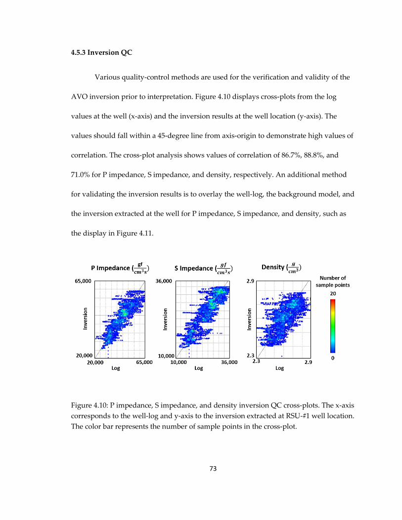
73
4.5.3 Inversion QC
Various quality-control methods are used for the verification and validity of the
AVO inversion prior to interpretation. Figure 4.10 displays cross-plots from the log
values at the well (x-axis) and the inversion results at the well location (y-axis). The
values should fall within a 45-degree line from axis-origin to demonstrate high values of
correlation. The cross-plot analysis shows values of correlation of 86.7%, 88.8%, and
71.0% for P impedance, S impedance, and density, respectively. An additional method
for validating the inversion results is to overlay the well-log, the background model, and
the inversion extracted at the well for P impedance, S impedance, and density, such as
the display in Figure 4.11.
Figure 4.10: P impedance, S impedance, and density inversion QC cross-plots. The x-axis
corresponds to the well-log and y-axis to the inversion extracted at RSU-#1 well location.
The color bar represents the number of sample points in the cross-plot.
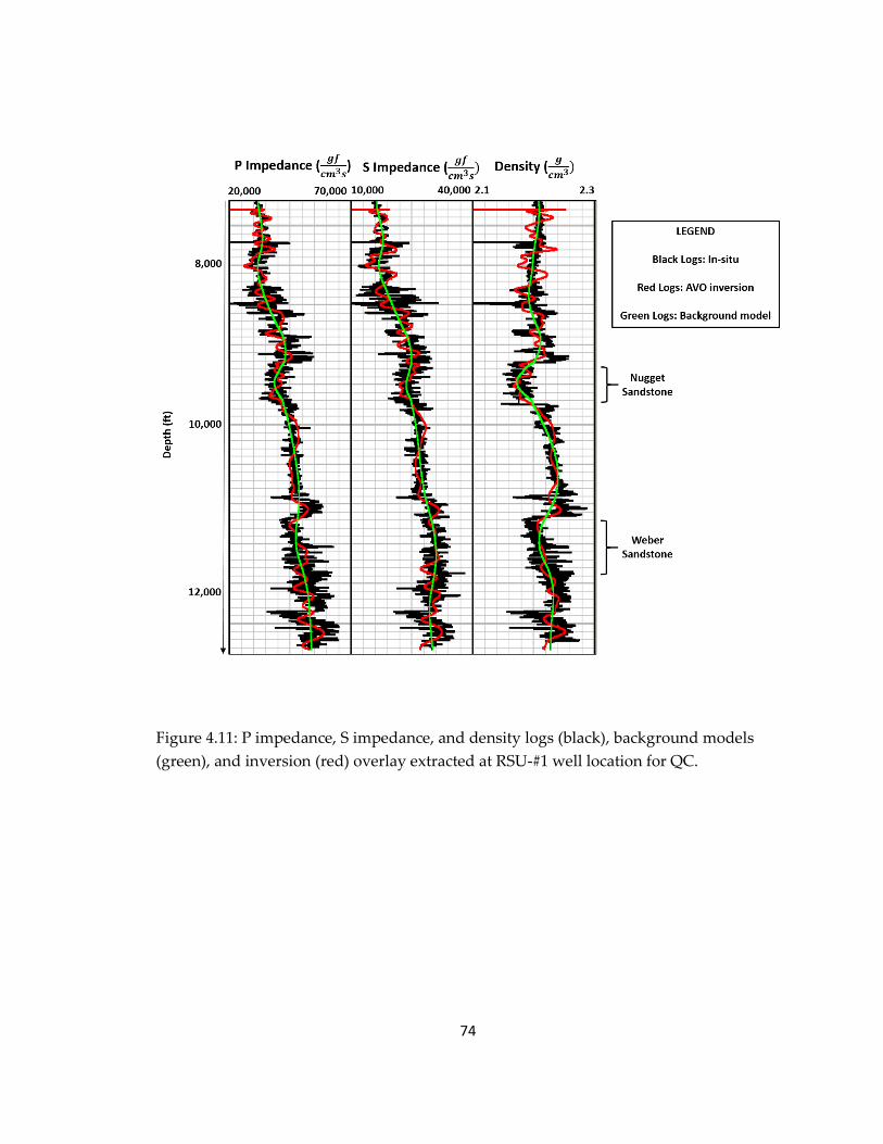
74
Figure 4.11: P impedance, S impedance, and density logs (black), background models
(green), and inversion (red) overlay extracted at RSU-#1 well location for QC.
75
Chapter 5
PS reflections seismic processing and
inversion
Although the industry standard is to analyze the vertical component (PP
reflection) data, converted-wave reflections (PS mode conversion) can be used to help
determine additional information such as density with higher reliability due to the
sensitive variations of the S-waves to density compared to the P-waves. Processing of the
horizontal component dataset requires having prior information regarding the static
solution and velocity model of the P-wave data. The PS processing sequence includes
steps for analysis of PP reflection data but involves some additional steps such as
component rotation, Asymmetrical Conversion Point (ACP) binning, Vp
Vs analysis, shear-
wave splitting analysis and rotation, and PP – PS event registration. The PS image is used
to generate the post-stack inversion to obtain a volume of S impedance, that is more
accurate than the one derived from the PP AVO inversion.
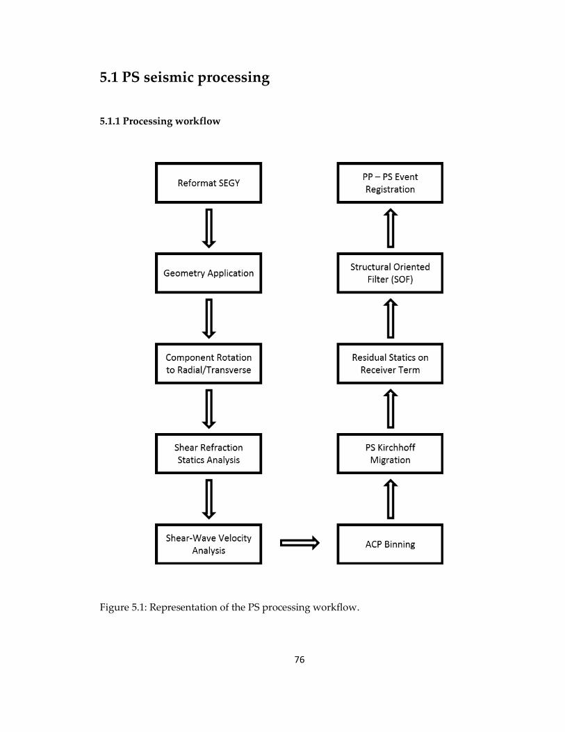
76
5.1 PS seismic processing
5.1.1 Processing workflow
Figure 5.1: Representation of the PS processing workflow.
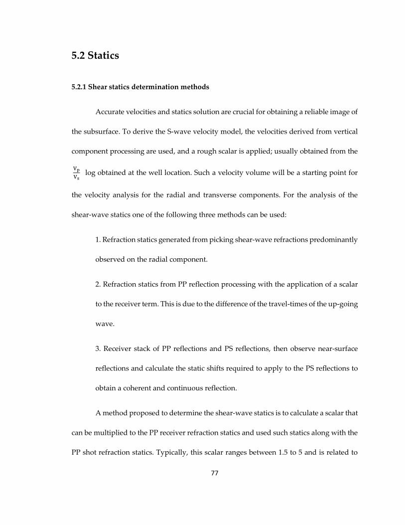
77
5.2 Statics
5.2.1 Shear statics determination methods
Accurate velocities and statics solution are crucial for obtaining a reliable image of
the subsurface. To derive the S-wave velocity model, the velocities derived from vertical
component processing are used, and a rough scalar is applied; usually obtained from the
Vp
Vs log obtained at the well location. Such a velocity volume will be a starting point for
the velocity analysis for the radial and transverse components. For the analysis of the
shear-wave statics one of the following three methods can be used:
1. Refraction statics generated from picking shear-wave refractions predominantly
observed on the radial component.
2. Refraction statics from PP reflection processing with the application of a scalar
to the receiver term. This is due to the difference of the travel-times of the up-going
wave.
3. Receiver stack of PP reflections and PS reflections, then observe near-surface
reflections and calculate the static shifts required to apply to the PS reflections to
obtain a coherent and continuous reflection.
A method proposed to determine the shear-wave statics is to calculate a scalar that
can be multiplied to the PP receiver refraction statics and used such statics along with the
PP shot refraction statics. Typically, this scalar ranges between 1.5 to 5 and is related to
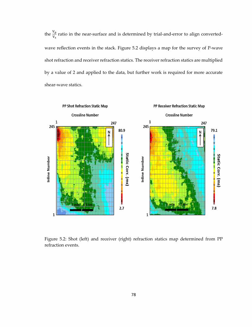
78
the Vp
Vs ratio in the near-surface and is determined by trial-and-error to align converted-
wave reflection events in the stack. Figure 5.2 displays a map for the survey of P-wave
shot refraction and receiver refraction statics. The receiver refraction statics are multiplied
by a value of 2 and applied to the data, but further work is required for more accurate
shear-wave statics.
Figure 5.2: Shot (left) and receiver (right) refraction statics map determined from PP
refraction events.
1.5 km 1 mile 1.5 km 1 mile
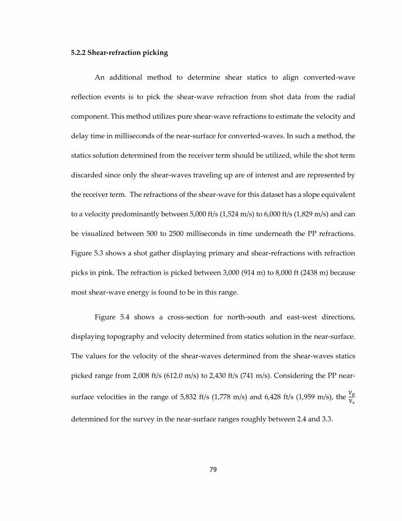
79
5.2.2 Shear-refraction picking
An additional method to determine shear statics to align converted-wave
reflection events is to pick the shear-wave refraction from shot data from the radial
component. This method utilizes pure shear-wave refractions to estimate the velocity and
delay time in milliseconds of the near-surface for converted-waves. In such a method, the
statics solution determined from the receiver term should be utilized, while the shot term
discarded since only the shear-waves traveling up are of interest and are represented by
the receiver term. The refractions of the shear-wave for this dataset has a slope equivalent
to a velocity predominantly between 5,000 ft/s (1,524 m/s) to 6,000 ft/s (1,829 m/s) and can
be visualized between 500 to 2500 milliseconds in time underneath the PP refractions.
Figure 5.3 shows a shot gather displaying primary and shear-refractions with refraction
picks in pink. The refraction is picked between 3,000 (914 m) to 8,000 ft (2438 m) because
most shear-wave energy is found to be in this range.
Figure 5.4 shows a cross-section for north-south and east-west directions,
displaying topography and velocity determined from statics solution in the near-surface.
The values for the velocity of the shear-waves determined from the shear-waves statics
picked range from 2,008 ft/s (612.0 m/s) to 2,430 ft/s (741 m/s). Considering the PP near-
surface velocities in the range of 5,832 ft/s (1,778 m/s) and 6,428 ft/s (1,959 m/s), the Vp
Vs
determined for the survey in the near-surface ranges roughly between 2.4 and 3.3.
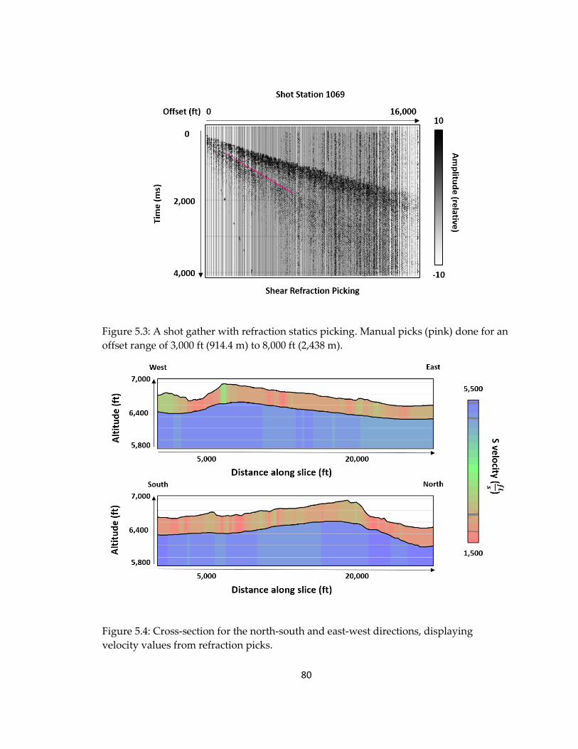
80
Figure 5.3: A shot gather with refraction statics picking. Manual picks (pink) done for an
offset range of 3,000 ft (914.4 m) to 8,000 ft (2,438 m).
Figure 5.4: Cross-section for the north-south and east-west directions, displaying
velocity values from refraction picks.
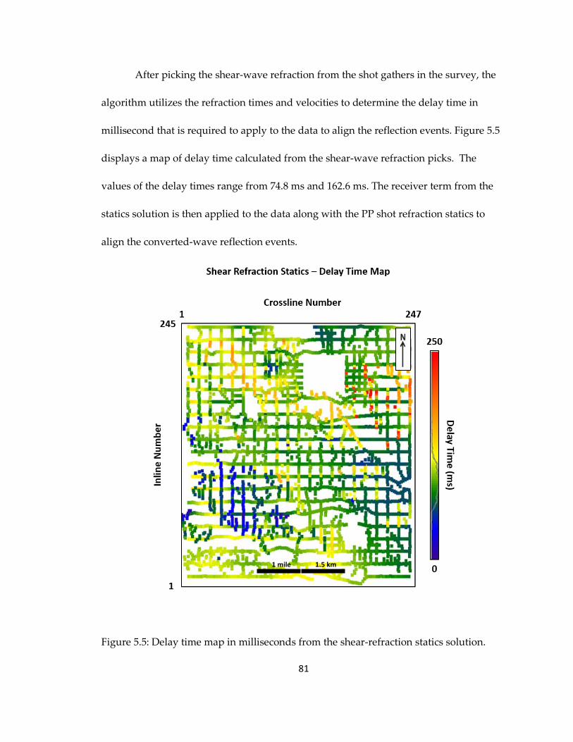
81
After picking the shear-wave refraction from the shot gathers in the survey, the
algorithm utilizes the refraction times and velocities to determine the delay time in
millisecond that is required to apply to the data to align the reflection events. Figure 5.5
displays a map of delay time calculated from the shear-wave refraction picks. The
values of the delay times range from 74.8 ms and 162.6 ms. The receiver term from the
statics solution is then applied to the data along with the PP shot refraction statics to
align the converted-wave reflection events.
Figure 5.5: Delay time map in milliseconds from the shear-refraction statics solution.
1.5 km 1 mile
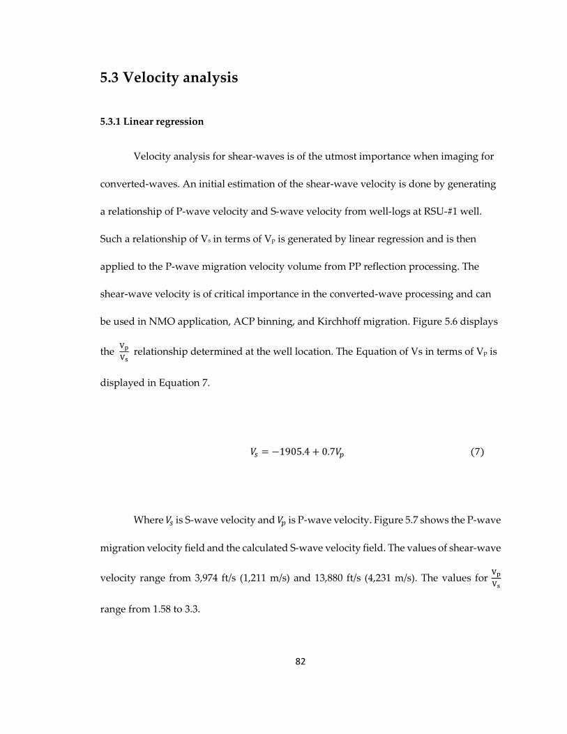
82
5.3 Velocity analysis
5.3.1 Linear regression
Velocity analysis for shear-waves is of the utmost importance when imaging for
converted-waves. An initial estimation of the shear-wave velocity is done by generating
a relationship of P-wave velocity and S-wave velocity from well-logs at RSU-#1 well.
Such a relationship of Vs in terms of Vp is generated by linear regression and is then
applied to the P-wave migration velocity volume from PP reflection processing. The
shear-wave velocity is of critical importance in the converted-wave processing and can
be used in NMO application, ACP binning, and Kirchhoff migration. Figure 5.6 displays
the Vp
Vs relationship determined at the well location. The Equation of Vs in terms of Vp is
displayed in Equation 7.
𝑉𝑠 = −1905.4 + 0.7𝑉𝑝 (7)
Where 𝑉𝑠 is S-wave velocity and 𝑉𝑝 is P-wave velocity. Figure 5.7 shows the P-wave
migration velocity field and the calculated S-wave velocity field. The values of shear-wave
velocity range from 3,974 ft/s (1,211 m/s) and 13,880 ft/s (4,231 m/s). The values for Vp
Vs
range from 1.58 to 3.3.
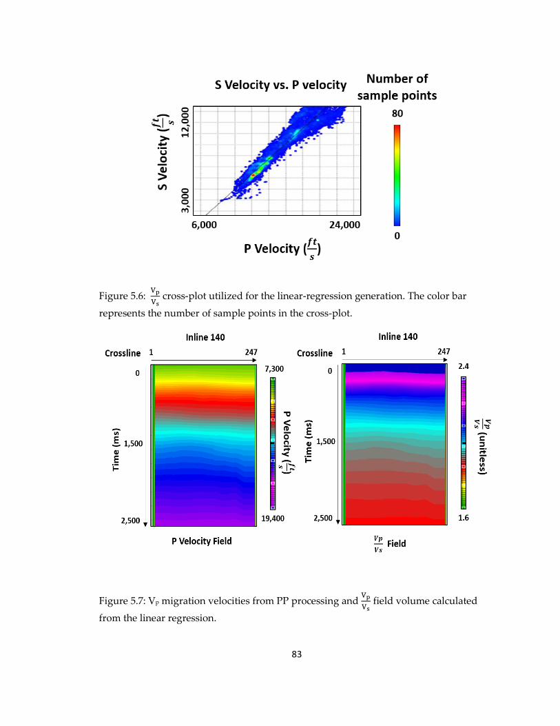
83
Figure 5.6: Vp
Vs cross-plot utilized for the linear-regression generation. The color bar
represents the number of sample points in the cross-plot.
Figure 5.7: Vp migration velocities from PP processing and Vp
Vs field volume calculated
from the linear regression.
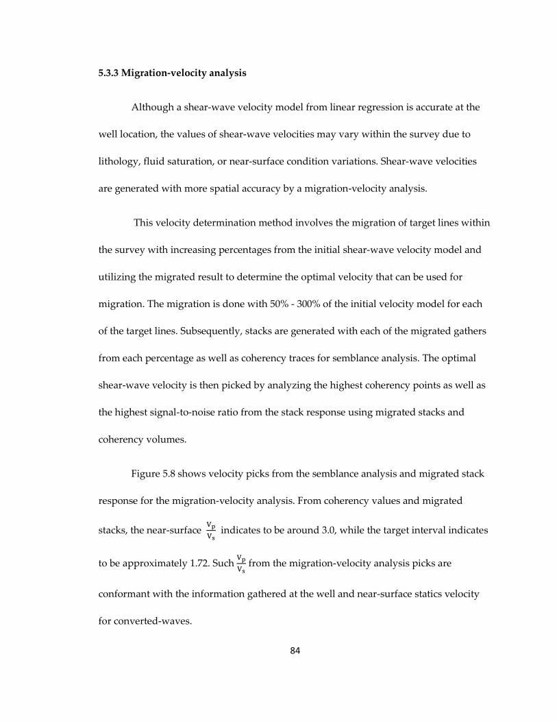
84
5.3.3 Migration-velocity analysis
Although a shear-wave velocity model from linear regression is accurate at the
well location, the values of shear-wave velocities may vary within the survey due to
lithology, fluid saturation, or near-surface condition variations. Shear-wave velocities
are generated with more spatial accuracy by a migration-velocity analysis.
This velocity determination method involves the migration of target lines within
the survey with increasing percentages from the initial shear-wave velocity model and
utilizing the migrated result to determine the optimal velocity that can be used for
migration. The migration is done with 50% - 300% of the initial velocity model for each
of the target lines. Subsequently, stacks are generated with each of the migrated gathers
from each percentage as well as coherency traces for semblance analysis. The optimal
shear-wave velocity is then picked by analyzing the highest coherency points as well as
the highest signal-to-noise ratio from the stack response using migrated stacks and
coherency volumes.
Figure 5.8 shows velocity picks from the semblance analysis and migrated stack
response for the migration-velocity analysis. From coherency values and migrated
stacks, the near-surface Vp
Vs indicates to be around 3.0, while the target interval indicates
to be approximately 1.72. Such Vp
Vs from the migration-velocity analysis picks are
conformant with the information gathered at the well and near-surface statics velocity
for converted-waves.
85
Figure 5.8: Migration velocity analysis demonstrated from velocity picks from semblance analysis (left) and migrated stack
response (right).
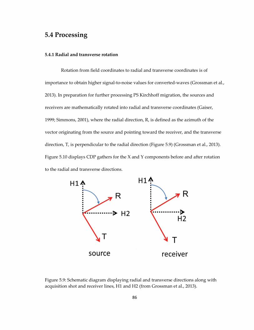
86
5.4 Processing
5.4.1 Radial and transverse rotation
Rotation from field coordinates to radial and transverse coordinates is of
importance to obtain higher signal-to-noise values for converted-waves (Grossman et al.,
2013). In preparation for further processing PS Kirchhoff migration, the sources and
receivers are mathematically rotated into radial and transverse coordinates (Gaiser,
1999; Simmons, 2001), where the radial direction, R, is defined as the azimuth of the
vector originating from the source and pointing toward the receiver, and the transverse
direction, T, is perpendicular to the radial direction (Figure 5.9) (Grossman et al., 2013).
Figure 5.10 displays CDP gathers for the X and Y components before and after rotation
to the radial and transverse directions.
Figure 5.9: Schematic diagram displaying radial and transverse directions along with
acquisition shot and receiver lines, H1 and H2 (from Grossman et al., 2013).
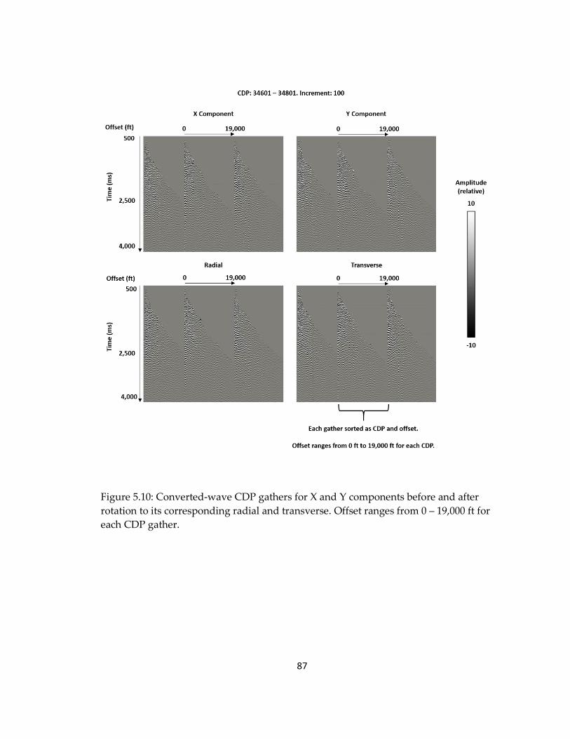
87
Figure 5.10: Converted-wave CDP gathers for X and Y components before and after
rotation to its corresponding radial and transverse. Offset ranges from 0 – 19,000 ft for
each CDP gather.

88
5.4.2 Converted-wave binning
For an earth model with flat layers, the PP reflection points coincide with the
midpoint locations (CMP), whereas, the PS conversion points do not. As a direct
consequence, the notion of a CMP gather based on sorting PP data from acquisition
coordinates does not apply to PS seismic data. Instead, a Common Conversion Point
(CCP) sorting is done for PS data that gathers traces in the same conversion point
coordinate. An essential aspect of CCP sorting is that the asymmetric ray path associated
with the PS reflection gives rise to a periodic variation in the fold of the CCP gathers. At
infinite depth, the CCP reaches an asymptotic conversion point (ACP) coordinate with
respect to the source location (Figure 5.11) (Tessmer and Behle, 1988). ACP binning is
done to the radial and transverse seismic volumes by using the P and S-wave velocities.
Figure 5.11: Schematic diagram showing the CMP, CCP, and ACP coordinates for a
source and receiver pair (modified from Tessmer and Behle, 1988).
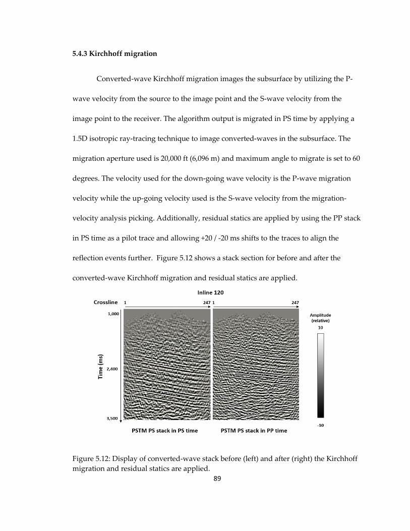
89
5.4.3 Kirchhoff migration
Converted-wave Kirchhoff migration images the subsurface by utilizing the P-
wave velocity from the source to the image point and the S-wave velocity from the
image point to the receiver. The algorithm output is migrated in PS time by applying a
1.5D isotropic ray-tracing technique to image converted-waves in the subsurface. The
migration aperture used is 20,000 ft (6,096 m) and maximum angle to migrate is set to 60
degrees. The velocity used for the down-going wave velocity is the P-wave migration
velocity while the up-going velocity used is the S-wave velocity from the migration-
velocity analysis picking. Additionally, residual statics are applied by using the PP stack
in PS time as a pilot trace and allowing +20 / -20 ms shifts to the traces to align the
reflection events further. Figure 5.12 shows a stack section for before and after the
converted-wave Kirchhoff migration and residual statics are applied.
Figure 5.12: Display of converted-wave stack before (left) and after (right) the Kirchhoff
migration and residual statics are applied.
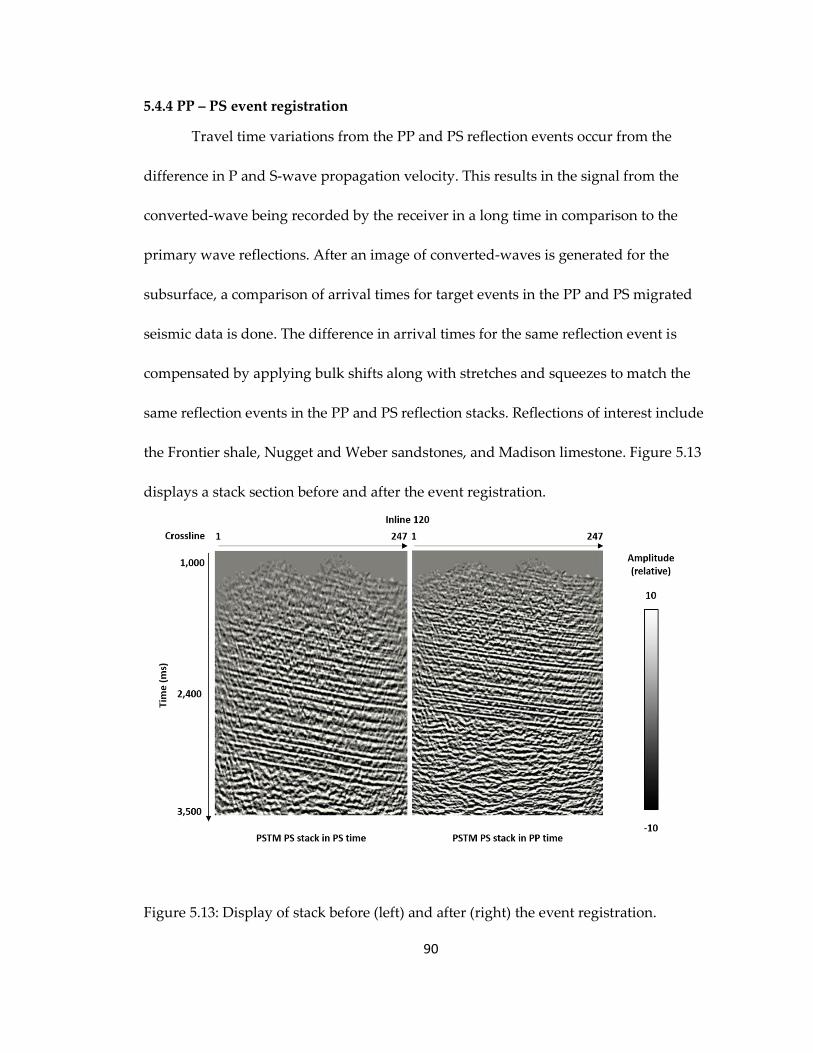
90
5.4.4 PP – PS event registration
Travel time variations from the PP and PS reflection events occur from the
difference in P and S-wave propagation velocity. This results in the signal from the
converted-wave being recorded by the receiver in a long time in comparison to the
primary wave reflections. After an image of converted-waves is generated for the
subsurface, a comparison of arrival times for target events in the PP and PS migrated
seismic data is done. The difference in arrival times for the same reflection event is
compensated by applying bulk shifts along with stretches and squeezes to match the
same reflection events in the PP and PS reflection stacks. Reflections of interest include
the Frontier shale, Nugget and Weber sandstones, and Madison limestone. Figure 5.13
displays a stack section before and after the event registration.
Figure 5.13: Display of stack before (left) and after (right) the event registration.
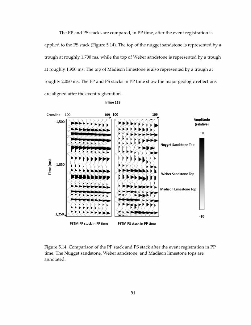
91
The PP and PS stacks are compared, in PP time, after the event registration is
applied to the PS stack (Figure 5.14). The top of the nugget sandstone is represented by a
trough at roughly 1,700 ms, while the top of Weber sandstone is represented by a trough
at roughly 1,950 ms. The top of Madison limestone is also represented by a trough at
roughly 2,050 ms. The PP and PS stacks in PP time show the major geologic reflections
are aligned after the event registration.
Figure 5.14: Comparison of the PP stack and PS stack after the event registration in PP
time. The Nugget sandstone, Weber sandstone, and Madison limestone tops are
annotated.
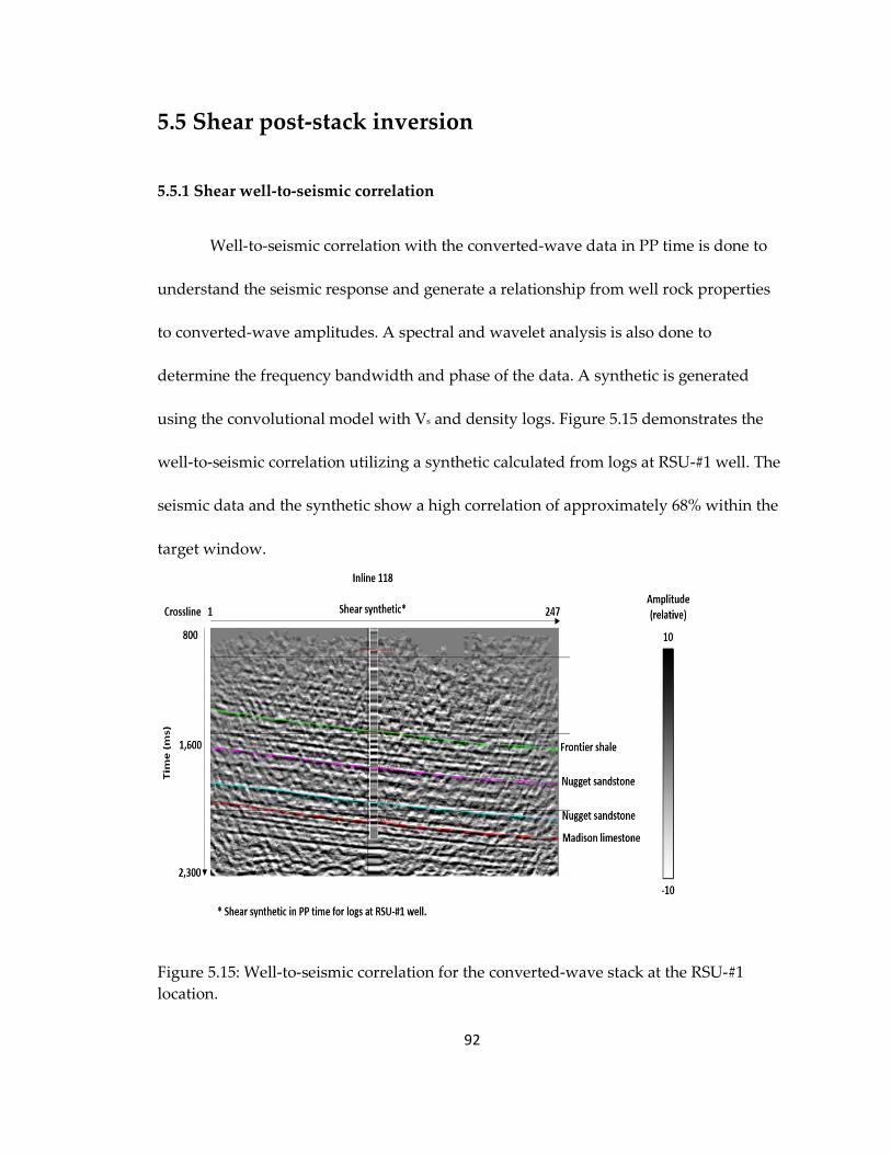
92
5.5 Shear post-stack inversion
5.5.1 Shear well-to-seismic correlation
Well-to-seismic correlation with the converted-wave data in PP time is done to
understand the seismic response and generate a relationship from well rock properties
to converted-wave amplitudes. A spectral and wavelet analysis is also done to
determine the frequency bandwidth and phase of the data. A synthetic is generated
using the convolutional model with Vs and density logs. Figure 5.15 demonstrates the
well-to-seismic correlation utilizing a synthetic calculated from logs at RSU-#1 well. The
seismic data and the synthetic show a high correlation of approximately 68% within the
target window.
Figure 5.15: Well-to-seismic correlation for the converted-wave stack at the RSU-#1
location.
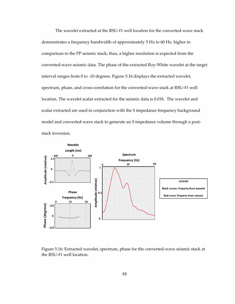
93
The wavelet extracted at the RSU-#1 well location for the converted-wave stack
demonstrates a frequency bandwidth of approximately 5 Hz to 60 Hz, higher in
comparison to the PP seismic stack; thus, a higher resolution is expected from the
converted-wave seismic data. The phase of the extracted Roy-White wavelet at the target
interval ranges from 0 to -10 degrees. Figure 5.16 displays the extracted wavelet,
spectrum, phase, and cross-correlation for the converted-wave stack at RSU-#1 well
location. The wavelet scalar extracted for the seismic data is 0.018. The wavelet and
scalar extracted are used in conjunction with the S impedance frequency background
model and converted-wave stack to generate an S impedance volume through a post-
stack inversion.
Figure 5.16: Extracted wavelet, spectrum, phase for the converted-wave seismic stack at
the RSU-#1 well location.

94
5.5.2 Post-stack inversion
Converted-wave post-stack inversion utilizes the stack section, S impedance
background model, extracted wavelet and scalars to generate a volume of shear
impedance. In a model-based inversion, a simple initial acoustic impedance model is
convolved with the wavelet to obtain a synthetic response that is compared with the
actual seismic trace. The impedance model is altered iteratively until the difference
between the inverted trace and the seismic trace is reduced to a threshold value (Veeken
and Da Silva, 2004). A model with a minimal difference is accepted as a solution. An
advantage of model-based inversion is that it gives satisfactory results, even with
limited well control and poor-quality seismic. The seismic dataset itself acts as the guide
for the inversion, and a wavelet can be easily derived straight from the seismic. The
least-squares inversion method is a type of model-based inversion where the threshold
value is the smallest least-squares error (Veeken and Da Silva, 2004).
Post-stack inversion for shear impedance is calculated by assuming the seismic
response of shear-shear reflections is characterized by the converted-wave data. Figure
5.17 shows a section of the shear impedance inversion at inline 118, the location of the
well RSU-#1. The values of the shear impedance range from 11,495 𝑔𝑓
𝑐𝑚3𝑠 and 31,368
𝑔𝑓
𝑐𝑚3𝑠.
The inversion volume is used to extract shear impedance RMS maps at the target
Nugget and Weber sandstones to determine anomalies that may be correlated to high-
porosity areas within the survey.

95
Figure 5.17: Shear impedance volume generated from the converted-wave seismic section. Shear impedance inversion volume
is displayed at the well RSU-#1 location.
96
Chapter 6
Interpretation
To characterize the reservoir and determine the potential volume for carbon
dioxide storage within the survey area, the outputs from the AVO inversion, calculated
elastic and seismic attributes, and azimuthal anisotropic analysis from velocity variations
with azimuth are analyzed together to gain insight into areas with increased void volume
within the target sandstones. A rock physics relationship is generated at the well to
determine porosity in terms of shear modulus, and such a relationship is applied to the
inversion volumes to obtain a spatial characterization of porosity. Porosity anomalies are
validated through multi-attribute analysis, and a regional stress field is derived from the
azimuthal anisotropic analysis. A location for carbon dioxide sequestration is proposed
within the Jim Bridger 3D survey area. A carbon dioxide injection model is created, and a
volumetric analysis is done to determine the potential capacity and possible duration of
carbon dioxide sequestration for the Jim Bridger power plant.
97
6.1 Porosity estimation
6.1.1 Linear regression
To estimate porosity, a linear regression is fit using various attributes derived from
the well-logs such as P impedance, S impedance, density, , and . Linear relationships
between porosity and such attributes are generated to identify the attribute pair
demonstrating the highest cross-correlation. Density is known to be highly correlated to
porosity values, but additional factors such as fluid saturation can alter this trend. The
cross-correlation of density and porosity from cross-plot analysis at the well is 66%.
As additional attributes are investigated, a normalized is determined to be
highly correlated with porosity values with a cross-correlation value of 93%. Since is
the product of squared shear impedance times density, the effect of fluid saturation is
neglected as S-waves do not propagate through fluids; thus, normalized is found to be
a reliable proxy for porosity values at the well-location, and such a derived relationship
can be applied to attributes obtained from the AVO pre-stack inversion. Equation 8
demonstrates the equation derived at the well location.
𝜙 = 0.25 − 0.0034μρ (8)
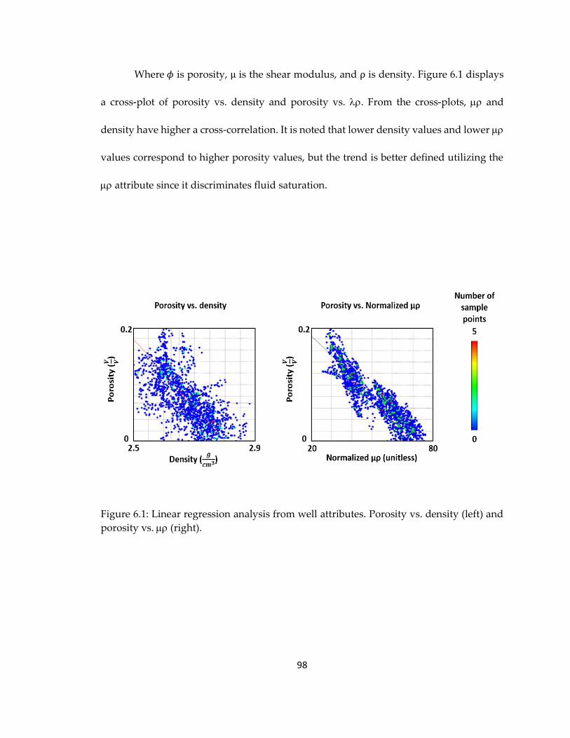
98
Where 𝜙 is porosity, μ is the shear modulus, and ρ is density. Figure 6.1 displays
a cross-plot of porosity vs. density and porosity vs. . From the cross-plots, and
density have higher a cross-correlation. It is noted that lower density values and lower
values correspond to higher porosity values, but the trend is better defined utilizing the
attribute since it discriminates fluid saturation.
Figure 6.1: Linear regression analysis from well attributes. Porosity vs. density (left) and
porosity vs. (right).

99
6.1.2 Porosity volume
The equation relating porosity to derived from the well, Equation 8, is applied
to the attribute obtained from the AVO pre-stack inversion to determine a porosity
volume. Figure 6.2 displays a porosity section from inline 118. The top and base horizons
for the Nugget and Weber sandstones are displayed on the section. These horizons are
picked to later obtain isopach maps of the target intervals for volumetric calculations of
CO2. The values from the porosity volume range from 5% to 22%. The Nugget sandstone
displays an average value of 16% porosity, while the Weber sandstone displays an
average value of 12% porosity.
Figure 6.2: Porosity section derived by applying the porosity – transform to the
volume from the AVO inversion. Top and base of the Nugget and Weber sandstone
horizons are displayed.

100
Equation 8 is also applied to the volume obtained from post-stack inversion
from the PS stack in PP time. Shear-waves have a higher sensitivity to the rock matrix and
are not influenced by the saturating fluid within the formation; thus, the resultant porosity
volume obtained from PS post-stack inversion is potentially more accurate. Figure 6.3
displays the porosity volume obtained from the S impedance post-stack inversion. The
porosity volume also displays higher resolution that could aid in the interpretation for
CCS.
Figure 6.3: Porosity section derived by applying the porosity – transform to the
volume from the PS post-stack inversion. Frontier shale, Nugget and Weber sandstones,
and Madison limestone horizons are displayed.
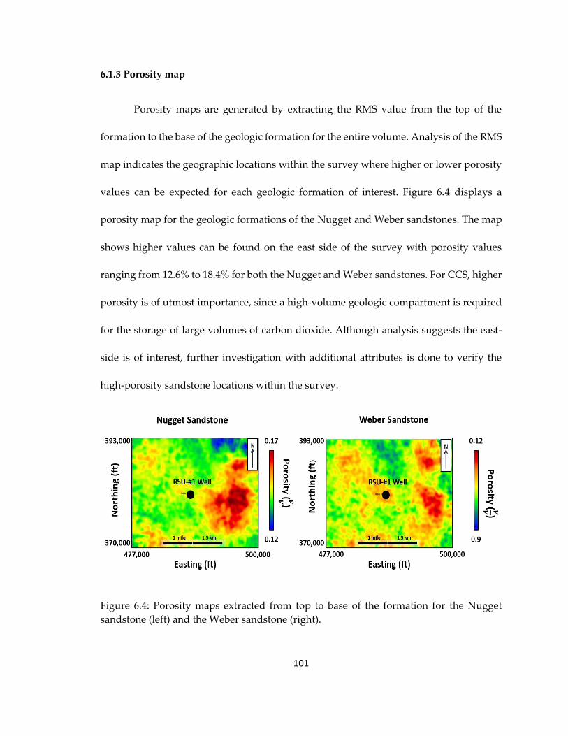
101
6.1.3 Porosity map
Porosity maps are generated by extracting the RMS value from the top of the
formation to the base of the geologic formation for the entire volume. Analysis of the RMS
map indicates the geographic locations within the survey where higher or lower porosity
values can be expected for each geologic formation of interest. Figure 6.4 displays a
porosity map for the geologic formations of the Nugget and Weber sandstones. The map
shows higher values can be found on the east side of the survey with porosity values
ranging from 12.6% to 18.4% for both the Nugget and Weber sandstones. For CCS, higher
porosity is of utmost importance, since a high-volume geologic compartment is required
for the storage of large volumes of carbon dioxide. Although analysis suggests the east-
side is of interest, further investigation with additional attributes is done to verify the
high-porosity sandstone locations within the survey.
Figure 6.4: Porosity maps extracted from top to base of the formation for the Nugget
sandstone (left) and the Weber sandstone (right).

102
6.2 Attribute volumes
6.2.1 and
and attributes are indicators of fluid saturation, lithology, and rock
properties. is inherently indicative of fluid saturation since it largely uses information
from P-wave propagation, which is profoundly affected by fluid saturation. On the other
hand, is a function of the matrix, which is not affected by fluid saturation within the
rock’s pores and is thus a proxy for lithology and high porosity. Attributes of and
are extracted for the formation interval for both Nugget and Weber sandstones. Figure 6.5
displays extracted RMS maps for the Nugget sandstone for and . Higher values of
and lower values of are observed in the east-side of the survey, suggesting higher
reservoir quality lithology.
Figure 6.5: and map for the Nugget sandstone interval.
103
6.2.2 Gradient and fluid factor
The AVO gradient and fluid factor are pre-stack derived attributes that can
indicate high-porosity sandstones and fluid saturation type (Jensen et al., 2016). Both
seismic attributes take advantage of the AVO effect for the reflection events and can
indicate fluid saturation and rock properties.
The Gradient (G) can be estimated from seismic data by a least-squares regression
applied to constant time slices of moveout corrected common reflection point gathers.
Care must be taken when determining the G to avoid bias caused by the curvature term
either by excluding large angles, typically above 30o, or by using a 3-term fit and
discarding the third term (Wiggins et al., 1985; Aki and Richards, 2002). Aki-Richards
linearization of the Zoeppritz equation is demonstrated by Equation 9. The gradient is the
second term, B, which is used as an attribute with information regarding Vp, Vs, and
density. Where 𝑘 is a constant.
𝑅(𝜃) ≈ 𝐴 + 𝐵𝑠𝑖𝑛2𝜃 + 𝐶𝑠𝑖𝑛2𝜃𝑡𝑎𝑛2𝜃 (9)
Where
𝐴 =1
2(
∆𝑉𝑝
𝑉𝑝+
∆𝜌
𝜌) 𝐵 =
∆𝑉𝑝
2𝑉𝑝− 4𝑘 (
∆𝑉𝑠
𝑉𝑠) − 2𝑘 (
∆𝜌
𝜌) 𝐶 =
∆𝑉𝑝
2𝑉𝑝
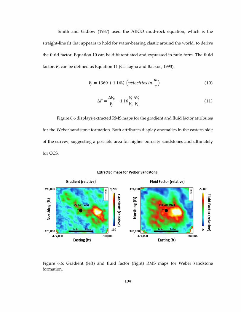
104
Smith and Gidlow (1987) used the ARCO mud-rock equation, which is the
straight-line fit that appears to hold for water-bearing clastic around the world, to derive
the fluid factor. Equation 10 can be differentiated and expressed in ratio form. The fluid
factor, 𝐹, can be defined as Equation 11 (Castagna and Backus, 1993).
𝑉𝑝 = 1360 + 1.16𝑉𝑠 (𝑣𝑒𝑙𝑜𝑐𝑖𝑡𝑖𝑒𝑠 𝑖𝑛 𝑚
𝑠) (10)
∆𝐹 =∆𝑉𝑝
𝑉𝑝− 1.16
𝑉𝑠
𝑉𝑝
∆𝑉𝑠
𝑉𝑠 (11)
Figure 6.6 displays extracted RMS maps for the gradient and fluid factor attributes
for the Weber sandstone formation. Both attributes display anomalies in the eastern side
of the survey, suggesting a possible area for higher porosity sandstones and ultimately
for CCS.
Figure 6.6: Gradient (left) and fluid factor (right) RMS maps for Weber sandstone
formation.
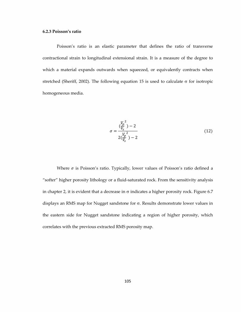
105
6.2.3 Poisson’s ratio
Poisson’s ratio is an elastic parameter that defines the ratio of transverse
contractional strain to longitudinal extensional strain. It is a measure of the degree to
which a material expands outwards when squeezed, or equivalently contracts when
stretched (Sheriff, 2002). The following equation 15 is used to calculate for isotropic
homogeneous media.
𝜎 =(𝑉𝑝
𝑉𝑠
2
) − 2
2(𝑉𝑝
𝑉𝑠
2
) − 2
(12)
Where 𝜎 is Poisson’s ratio. Typically, lower values of Poisson’s ratio defined a
“softer” higher porosity lithology or a fluid-saturated rock. From the sensitivity analysis
in chapter 2, it is evident that a decrease in indicates a higher porosity rock. Figure 6.7
displays an RMS map for Nugget sandstone for . Results demonstrate lower values in
the eastern side for Nugget sandstone indicating a region of higher porosity, which
correlates with the previous extracted RMS porosity map.
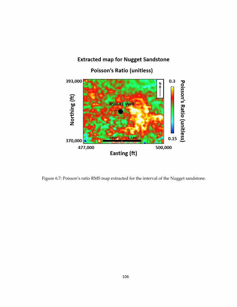
106
Figure 6.7: Poisson’s ratio RMS map extracted for the interval of the Nugget sandstone.
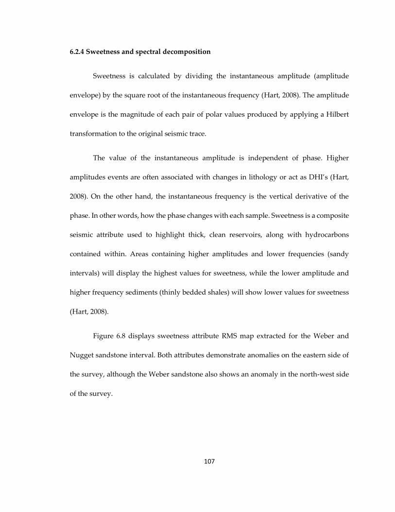
107
6.2.4 Sweetness and spectral decomposition
Sweetness is calculated by dividing the instantaneous amplitude (amplitude
envelope) by the square root of the instantaneous frequency (Hart, 2008). The amplitude
envelope is the magnitude of each pair of polar values produced by applying a Hilbert
transformation to the original seismic trace.
The value of the instantaneous amplitude is independent of phase. Higher
amplitudes events are often associated with changes in lithology or act as DHI’s (Hart,
2008). On the other hand, the instantaneous frequency is the vertical derivative of the
phase. In other words, how the phase changes with each sample. Sweetness is a composite
seismic attribute used to highlight thick, clean reservoirs, along with hydrocarbons
contained within. Areas containing higher amplitudes and lower frequencies (sandy
intervals) will display the highest values for sweetness, while the lower amplitude and
higher frequency sediments (thinly bedded shales) will show lower values for sweetness
(Hart, 2008).
Figure 6.8 displays sweetness attribute RMS map extracted for the Weber and
Nugget sandstone interval. Both attributes demonstrate anomalies on the eastern side of
the survey, although the Weber sandstone also shows an anomaly in the north-west side
of the survey.

108
Figure 6.8: Sweetness attribute RMS map extracted for Nugget and Weber sandstone
interval.
Additionally, spectral decomposition attributes are employed to decompose the
data into multiple frequencies to investigate anomalies at different bandwidths. In this
study, a spectral decomposition for 10 Hz, 30 Hz, and 50 Hz are computed, and RMS maps
are extracted for the Nugget and Weber sandstones. Figure 6.9 displays the spectral
decomposition RMS maps extracted. The nugget sandstone displays anomalies
predominantly in the eastern side of the survey throughout all frequencies. Other
anomalies also appear in the south-western side of the survey. For the Weber sandstone,
the 10 Hz map shows an anomaly in the south-west side of the survey while the higher
frequencies display anomalies in the eastern side of the survey. This suggests a possible
hydrocarbon saturated area with lower frequency content in the south-western corner of
the survey while a higher porosity area on the eastern side of the survey.
109
Figure 6.9: Spectral decomposition for 10, 20, 30 Hz for the Nugget and Weber sandstones, respectively.
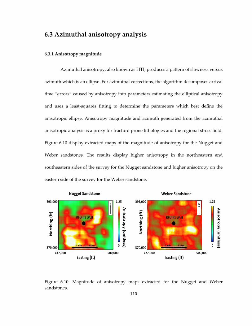
110
6.3 Azimuthal anisotropy analysis
6.3.1 Anisotropy magnitude
Azimuthal anisotropy, also known as HTI, produces a pattern of slowness versus
azimuth which is an ellipse. For azimuthal corrections, the algorithm decomposes arrival
time “errors” caused by anisotropy into parameters estimating the elliptical anisotropy
and uses a least-squares fitting to determine the parameters which best define the
anisotropic ellipse. Anisotropy magnitude and azimuth generated from the azimuthal
anisotropic analysis is a proxy for fracture-prone lithologies and the regional stress field.
Figure 6.10 display extracted maps of the magnitude of anisotropy for the Nugget and
Weber sandstones. The results display higher anisotropy in the northeastern and
southeastern sides of the survey for the Nugget sandstone and higher anisotropy on the
eastern side of the survey for the Weber sandstone.
Figure 6.10: Magnitude of anisotropy maps extracted for the Nugget and Weber
sandstones.
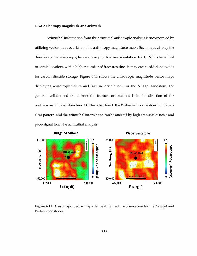
111
6.3.2 Anisotropy magnitude and azimuth
Azimuthal information from the azimuthal anisotropic analysis is incorporated by
utilizing vector maps overlain on the anisotropy magnitude maps. Such maps display the
direction of the anisotropy, hence a proxy for fracture orientation. For CCS, it is beneficial
to obtain locations with a higher number of fractures since it may create additional voids
for carbon dioxide storage. Figure 6.11 shows the anisotropic magnitude vector maps
displaying anisotropy values and fracture orientation. For the Nugget sandstone, the
general well-defined trend from the fracture orientations is in the direction of the
northeast-southwest direction. On the other hand, the Weber sandstone does not have a
clear pattern, and the azimuthal information can be affected by high amounts of noise and
poor-signal from the azimuthal analysis.
Figure 6.11: Anisotropic vector maps delineating fracture orientation for the Nugget and
Weber sandstones.
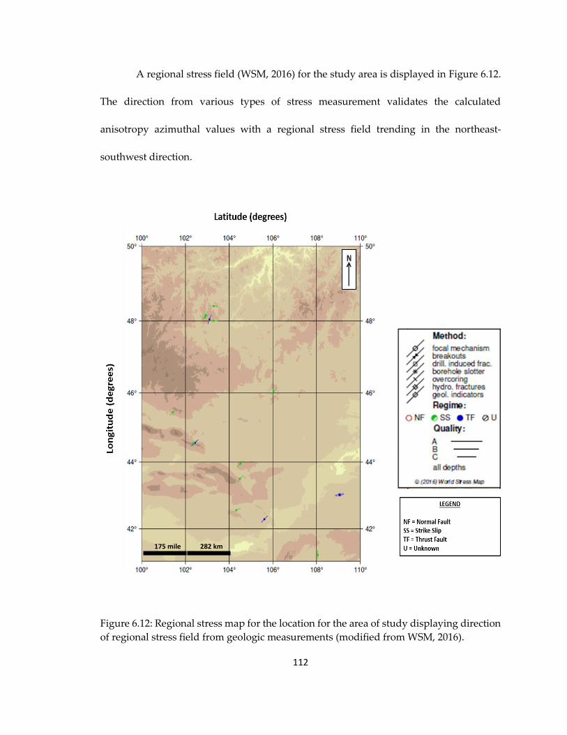
112
A regional stress field (WSM, 2016) for the study area is displayed in Figure 6.12.
The direction from various types of stress measurement validates the calculated
anisotropy azimuthal values with a regional stress field trending in the northeast-
southwest direction.
Figure 6.12: Regional stress map for the location for the area of study displaying direction
of regional stress field from geologic measurements (modified from WSM, 2016).
282 km 175 mile
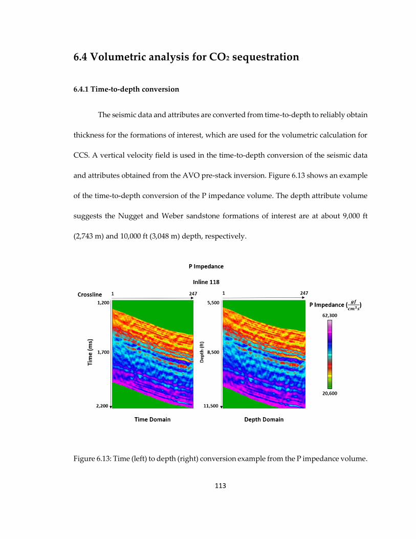
113
6.4 Volumetric analysis for CO2 sequestration
6.4.1 Time-to-depth conversion
The seismic data and attributes are converted from time-to-depth to reliably obtain
thickness for the formations of interest, which are used for the volumetric calculation for
CCS. A vertical velocity field is used in the time-to-depth conversion of the seismic data
and attributes obtained from the AVO pre-stack inversion. Figure 6.13 shows an example
of the time-to-depth conversion of the P impedance volume. The depth attribute volume
suggests the Nugget and Weber sandstone formations of interest are at about 9,000 ft
(2,743 m) and 10,000 ft (3,048 m) depth, respectively.
Figure 6.13: Time (left) to depth (right) conversion example from the P impedance volume.
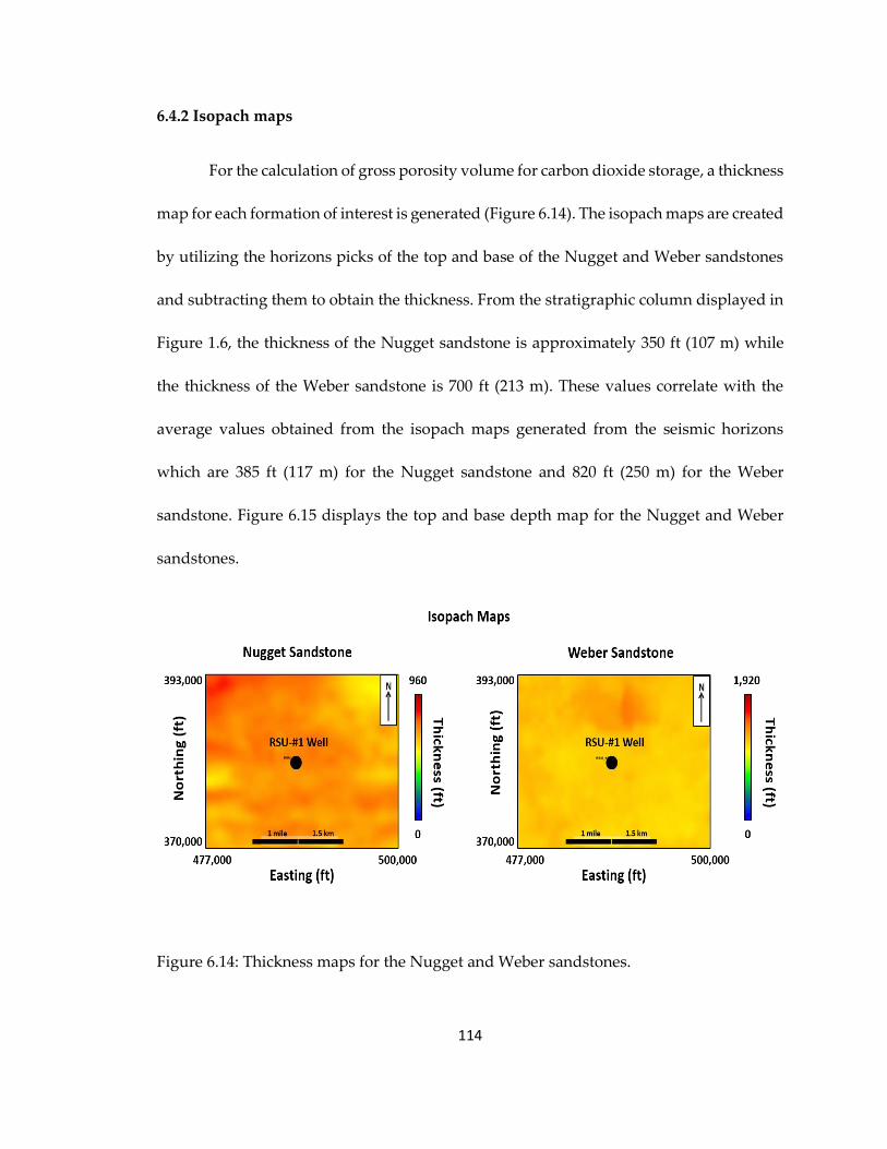
114
6.4.2 Isopach maps
For the calculation of gross porosity volume for carbon dioxide storage, a thickness
map for each formation of interest is generated (Figure 6.14). The isopach maps are created
by utilizing the horizons picks of the top and base of the Nugget and Weber sandstones
and subtracting them to obtain the thickness. From the stratigraphic column displayed in
Figure 1.6, the thickness of the Nugget sandstone is approximately 350 ft (107 m) while
the thickness of the Weber sandstone is 700 ft (213 m). These values correlate with the
average values obtained from the isopach maps generated from the seismic horizons
which are 385 ft (117 m) for the Nugget sandstone and 820 ft (250 m) for the Weber
sandstone. Figure 6.15 displays the top and base depth map for the Nugget and Weber
sandstones.
Figure 6.14: Thickness maps for the Nugget and Weber sandstones.
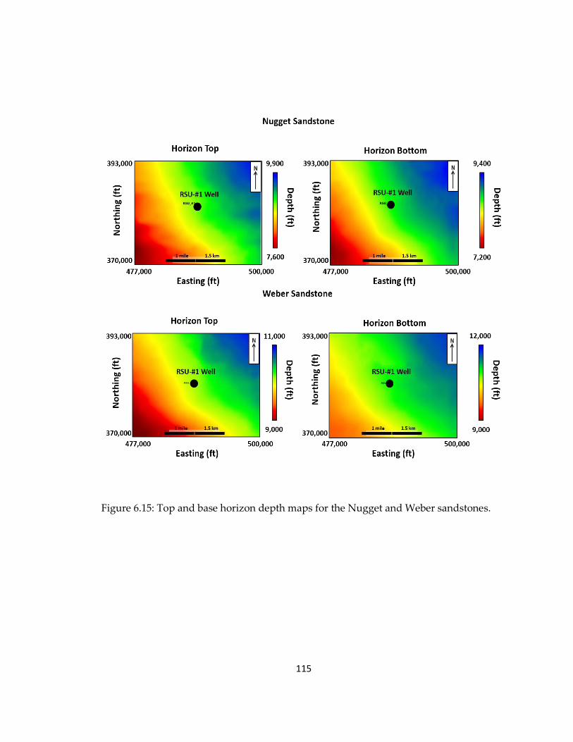
115
Figure 6.15: Top and base horizon depth maps for the Nugget and Weber sandstones.
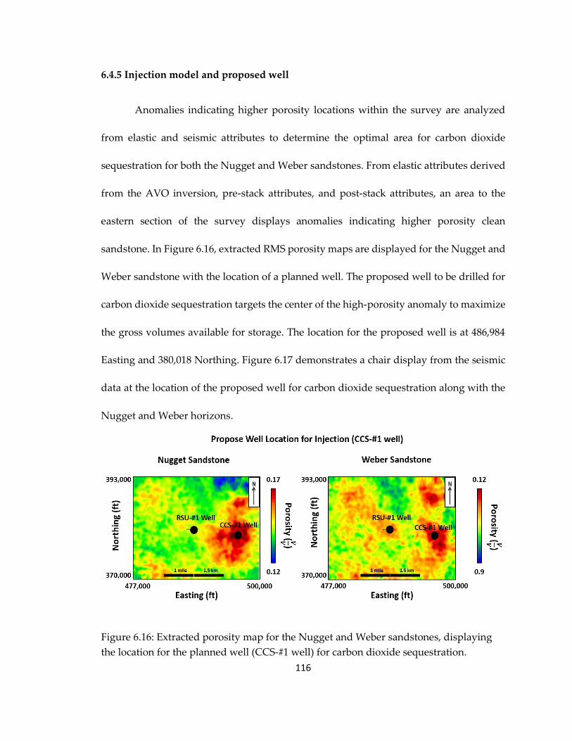
116
6.4.5 Injection model and proposed well
Anomalies indicating higher porosity locations within the survey are analyzed
from elastic and seismic attributes to determine the optimal area for carbon dioxide
sequestration for both the Nugget and Weber sandstones. From elastic attributes derived
from the AVO inversion, pre-stack attributes, and post-stack attributes, an area to the
eastern section of the survey displays anomalies indicating higher porosity clean
sandstone. In Figure 6.16, extracted RMS porosity maps are displayed for the Nugget and
Weber sandstone with the location of a planned well. The proposed well to be drilled for
carbon dioxide sequestration targets the center of the high-porosity anomaly to maximize
the gross volumes available for storage. The location for the proposed well is at 486,984
Easting and 380,018 Northing. Figure 6.17 demonstrates a chair display from the seismic
data at the location of the proposed well for carbon dioxide sequestration along with the
Nugget and Weber horizons.
Figure 6.16: Extracted porosity map for the Nugget and Weber sandstones, displaying
the location for the planned well (CCS-#1 well) for carbon dioxide sequestration.
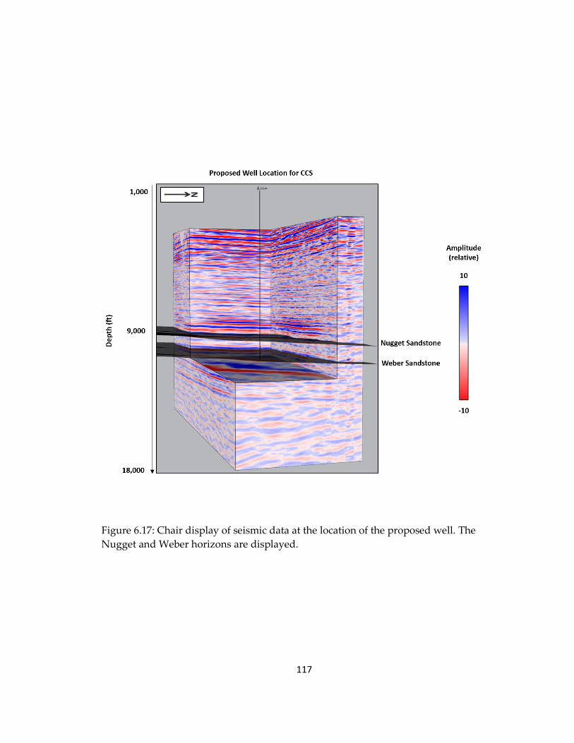
117
Figure 6.17: Chair display of seismic data at the location of the proposed well. The
Nugget and Weber horizons are displayed.

118
6.4.3 Volumetric assessment
For the high-porosity anomaly determined from the RMS porosity maps extracted,
areas can be analyzed for the estimation of low, middle, and high probabilities of targeting
high-porosity in the Nugget and Weber sandstone. Such analysis is done by identifying
areas surrounding the well location pertaining to a small area with highest-valued
porosity anomaly and a large area with lower-valued porosity anomaly. This allows for
the derivation of a probability analysis where a range of high to mid to low amount of
volume available for carbon storage. The cases where the probability of finding high-
porosity and low-porosity values within the sandstone are called P90 for 90% and P30 for
30% likeliness of a high-porosity sandstone. The case of 60% likeliness is in between and
is called P60 case. Figure 6.18 displays porosity maps for Nugget and Weber sandstones
with areas of 30%, 60%, and 90% likeliness of obtaining high-porosity values. Table 6.1
shows the values calculated estimated CO2 mass for storage capacity in Mt for the Weber
and Nugget sandstones. The P90, P60, and P30 for the Weber sandstone are 330.4 Mt, 176.7
Mt, and 61.9 Mt, respectively. On the other hand, for the estimates of mass for storage of
the Nugget sandstone are 231.2 Mt, 94.4Mt, and 57.7 Mt for the P90, 60, and P30 cases.
Table 6.1: Estimated carbon dioxide mass for storage capacity in Mt
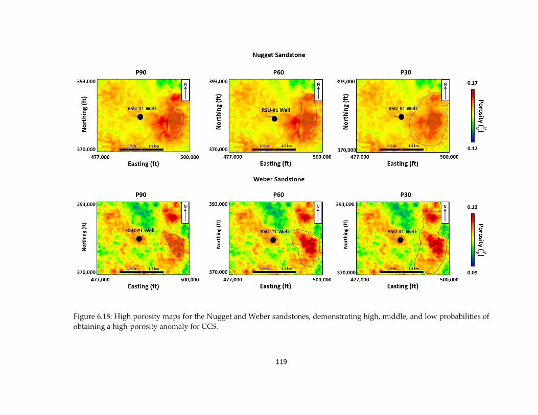
119
Figure 6.18: High porosity maps for the Nugget and Weber sandstones, demonstrating high, middle, and low probabilities of
obtaining a high-porosity anomaly for CCS.
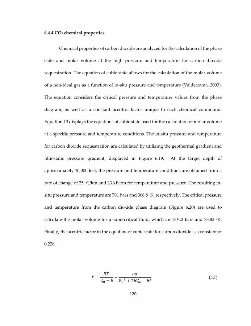
120
6.4.4 CO2 chemical properties
Chemical properties of carbon dioxide are analyzed for the calculation of the phase
state and molar volume at the high pressure and temperature for carbon dioxide
sequestration. The equation of cubic state allows for the calculation of the molar volume
of a non-ideal gas as a function of in-situ pressure and temperature (Valderrama, 2003).
The equation considers the critical pressure and temperature values from the phase
diagram, as well as a constant acentric factor unique to each chemical compound.
Equation 13 displays the equations of cubic state used for the calculation of molar volume
at a specific pressure and temperature conditions. The in-situ pressure and temperature
for carbon dioxide sequestration are calculated by utilizing the geothermal gradient and
lithostatic pressure gradient, displayed in Figure 6.19. At the target depth of
approximately 10,000 feet, the pressure and temperature conditions are obtained from a
rate of change of 25 oC/km and 23 kPa/m for temperature and pressure. The resulting in-
situ pressure and temperature are 701 bars and 366.8 oK, respectively. The critical pressure
and temperature from the carbon dioxide phase diagram (Figure 6.20) are used to
calculate the molar volume for a supercritical fluid, which are 304.2 bars and 73.82 oK.
Finally, the acentric factor in the equation of cubic state for carbon dioxide is a constant of
0.228.
𝑃 =𝑅𝑇
𝑉𝑚 − 𝑏−
𝑎𝛼
𝑉𝑚2 + 2𝑏𝑉𝑚 − 𝑏2
(13)
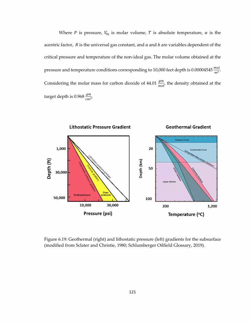
121
Where 𝑃 is pressure, 𝑉𝑚 is molar volume, 𝑇 is absolute temperature, 𝛼 is the
acentric factor, 𝑅 is the universal gas constant, and 𝑎 and 𝑏 are variables dependent of the
critical pressure and temperature of the non-ideal gas. The molar volume obtained at the
pressure and temperature conditions corresponding to 10,000 feet depth is 0.00004545 𝑚𝑜𝑙
𝑚3 .
Considering the molar mass for carbon dioxide of 44.01 𝑔𝑚
𝑚𝑜𝑙, the density obtained at the
target depth is 0.968 𝑔𝑚
𝑐𝑚3.
Figure 6.19: Geothermal (right) and lithostatic pressure (left) gradients for the subsurface
(modified from Sclater and Christie, 1980; Schlumberger Oilfield Glossary, 2019).
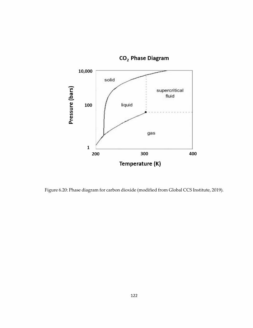
122
Figure 6.20: Phase diagram for carbon dioxide (modified from Global CCS Institute, 2019).
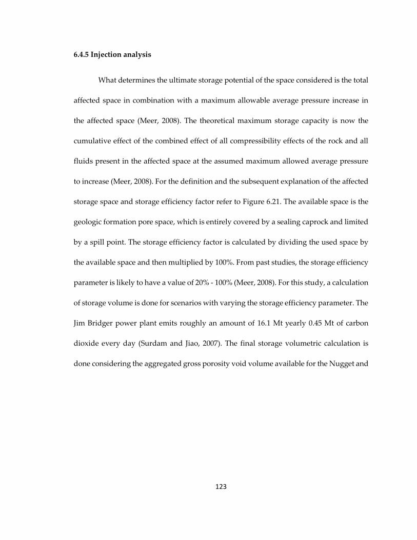
123
6.4.5 Injection analysis
What determines the ultimate storage potential of the space considered is the total
affected space in combination with a maximum allowable average pressure increase in
the affected space (Meer, 2008). The theoretical maximum storage capacity is now the
cumulative effect of the combined effect of all compressibility effects of the rock and all
fluids present in the affected space at the assumed maximum allowed average pressure
to increase (Meer, 2008). For the definition and the subsequent explanation of the affected
storage space and storage efficiency factor refer to Figure 6.21. The available space is the
geologic formation pore space, which is entirely covered by a sealing caprock and limited
by a spill point. The storage efficiency factor is calculated by dividing the used space by
the available space and then multiplied by 100%. From past studies, the storage efficiency
parameter is likely to have a value of 20% - 100% (Meer, 2008). For this study, a calculation
of storage volume is done for scenarios with varying the storage efficiency parameter. The
Jim Bridger power plant emits roughly an amount of 16.1 Mt yearly 0.45 Mt of carbon
dioxide every day (Surdam and Jiao, 2007). The final storage volumetric calculation is
done considering the aggregated gross porosity void volume available for the Nugget and
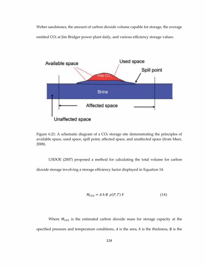
124
Weber sandstones, the amount of carbon dioxide volume capable for storage, the average
emitted CO2 at Jim Bridger power plant daily, and various efficiency storage values.
Figure 6.21: A schematic diagram of a CO2 storage site demonstrating the principles of
available space, used space, spill point, affected space, and unaffected space (from Meer,
2008).
USDOE (2007) proposed a method for calculating the total volume for carbon
dioxide storage involving a storage efficiency factor displayed in Equation 14.
𝑀𝐶𝑂2 = 𝐴 ℎ ∅ 𝜌(𝑃, 𝑇) 𝐸 (14)
Where 𝑀𝐶𝑂2 is the estimated carbon dioxide mass for storage capacity at the
specified pressure and temperature conditions, 𝐴 is the area, ℎ is the thickness, ∅ is the

125
effective porosity, 𝜌 is the density, P is pressure, T is temperature, and 𝐸 is the storage
efficiency factor which is a function of a capacity coefficient, permeability, and irreducible
water saturation (Juanes and Szulczewski, 2010). Measured permeability in the Weber
sandstone ranges from 0.001 mD to 13.8 mD, with an average of 1.4 mD and the highest
permeability in the upper eolian unit (Grana et al., 2017). Using the permeability and
irreducible water saturation values for Weber sandstone and Madison limestone, Surdam
(2007) suggests the storage efficiency factor ranges from 0.1 to 0.8.
Table 6.1 shows the high and low estimates of mass for storage in Mt for Nugget
and Weber sandstones. The aggregated mass for storage of CO2 range from 119.6 Mt to
561.6 Mt. In this study, values of 0.2, 0.4, 0.6, 0.8, and 1.0 are used for the storage efficiency
factor. Table 6.2 displays mass for storage values for various storage efficiency factors.
The range of CO2 mass for storage capacity varies from 23.9 Mt to 561.6 Mt. Considering
the amount of carbon dioxide emitted yearly by the Jim Bridger power plant of 16.3 Mt,
the final calculations for the duration of sequestration are shown in Table 6.3. The
estimates suggest sequestration is plausible for a period of 2 years to 35 years for low-and-
high-storage capacities, respectively. The average duration for sequestration is 13 years.
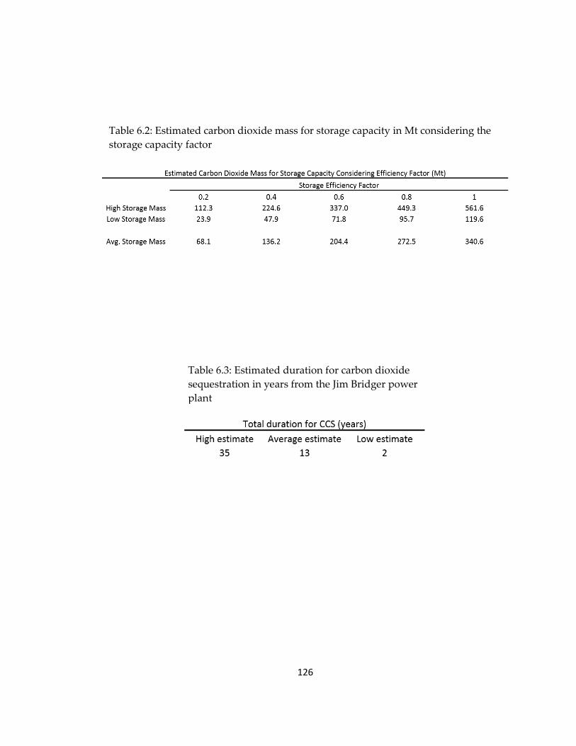
126
Table 6.3: Estimated duration for carbon dioxide
sequestration in years from the Jim Bridger power
plant
Table 6.2: Estimated carbon dioxide mass for storage capacity in Mt considering the
storage capacity factor
127
Chapter 7
Conclusions and future work
The goal of this thesis is to understand the relationship between rock properties
and their elastic response, petrophysical and rock physics analysis, seismic modeling, 3D-
3C processing, seismic inversion, and multi-attribute analysis are integrated to delimit
prospective areas with high-porosity content for carbon dioxide sequestration assessment.
What I have found is summarized below.
7.1 Conclusions
• Vertical geophone component is processed and split into 60 different OVTs for
application of Kirchhoff migration with 30,000 ft (9,144 m) aperture. By processing
the data in the OVT domain, the offsets and azimuths are preserved for further
analysis of anisotropy.
• Azimuthal anisotropy analysis is done by picking reflection events that show
velocity variations with azimuth when sorted as common offset – common
azimuth. Such events utilize the sinusoidal variation to solve the equation of an
ellipse and values of anisotropy can be estimated. The azimuthal anisotropic
128
analysis displays anisotropic magnitude between 0.6 – 1.2 and anisotropic azimuth
predominantly trends in the direction northeast-southwest (45 and 275 degrees)
for the Weber and Nugget sandstones. Results show areas of higher anisotropy
which could be a proxy for fractures within the sandstones that may be of interest
for carbon dioxide sequestration. The anisotropic azimuth is indicative of the
regional stress field and is validated by stress field data observed from geology in
the area. The localized stress field can be a proxy for fracture orientation.
• Structure-Oriented Filtering (SOF) is applied to OVT volumes to remove random
noise and improve reflection continuity and signal-to-noise values. SOF computes
structural coherence from the seismic trace within +6 ms to -6 ms and using a 5 by
5 grid of traces to apply a median filter which removes the incoherent noise
present. The algorithm is applied to offset vector tiles to avoid the mixing and
smoothing the azimuthal response used for the azimuthal analysis.
• VTI velocity analysis utilizing the method developed by Swan (2001) is done on
the CDP gathers post-migration to obtain velocity updates that flatten the gathers
from NI and G values. Three passes of 10% velocity variations are applied, and the
velocities within the Nugget and Weber sandstone formations are changed
between 50 – 200 m/s for improved flattened reflection events. The resulting
interval velocity field follows the geologic structure with higher continuity.
• Radon de-multiple is applied on the CDP gathers post-migration for the removal
of long-period multiples. A time-variant polygon cut is applied on the tau-p
129
domain calculated from the pre-stack data with an 80 ms taper. The resulting
gathers and stack show improved primary reflection event continuity, more
reliable AVO response, and decreased noise content for a better geologic and
amplitude anomaly interpretation.
• CDP domain noise attenuation is done by applying a mute on the frequency-
wavenumber domain to remove linear noise from the data. The algorithm applies
a mute in the f-k domain corresponding to velocity lower to 7,000 ft/s (2,134 m/s)
within the frequencies of 5 Hz – 35 Hz. An additional noise attenuation method in
CDP domain applied consists of transforming the data to the tau-p domain by a
Radon transform and applying a time-variant mute to keep only the primary
reflections. The data is transformed back to the space-time domain, and the
resulting traces are scaled down to 66.333% while the input is scaled down to
33.333% and both are added together. The resulting CDP gathers have coherent
and incoherent noise energy removed and improved signal-to-noise values.
• Angle ranges are analyzed on CDP gathers to determine the near, middle, and far
angle ranges with similar reflection coherency and signal-to-noise values for the
generation of angle stacks. The angle range analysis determined that angle stacks
00 – 13 degrees, 8 – 22 degrees, 18 – 32 degrees, and 28 – 42 degrees are optimal to
input into the AVO inversion algorithm. The signal-to-noise ratio and coherency
for the Nugget and Weber sandstone formations are similar throughout the angle

130
stacks with enough information in the far angles for the determination of the
density term.
• Seismic-to-well correlation utilizing the conditioned stack for the vertical
component data demonstrate the frequency and phase spectrum to be 5 Hz – 40
Hz and -50 degrees, respectively. Minor stretches and squeezes are made to match
the synthetics from the well to the seismic traces at the well location. The cross-
correlation is found to be at 80% within the target window from 1,400 ms to 2,000
ms. The Nugget and Weber sandstone’s seismic response is characterized and
matched by the synthetics from the well-logs.
• The seismic data is rotated to standard American SEGY polarity by applying a
phase rotation of 50 degrees to the CDP gathers prior to the calculation of the angle
stack. With zero phased angle stacks, wavelets are extracted for each one of the
angle stacks with its respective scalars for the AVO inversion. The wavelets
demonstrate to be consistently zero phased with +10 to -10 degree of error. The
scalars for the wavelets to match the seismic amplitude are 5.1e-05, 4.3e-05, 2.9e-
05, and 2.2e-05 for the near, middle, and far angle stacks, respectively.
• Low-frequency background models are generated by extrapolating well-log
values for P impedance, S impedance, and density throughout the whole survey
area guided by the Frontier shale, Weber sandstone, Nugget sandstone, and
Madison limestone seismic horizons. The extrapolation is done by a cokriging
algorithm that utilizes the well-logs values and the interval seismic velocities for
131
the guidance of the values for the survey area. The calculated models are then
smoothed to the missing frequencies from the seismic data by applying a high-cut
filter of 0 – 0 – 6 -12 Hz.
• Pre-stack simultaneous AVO inversion is a Bayesian algorithm used to generate
volumes of P impedance, S impedance, and density derived from the seismic data.
The inversion shows values for the Nugget and Weber sandstones to range for P
impedance, S impedance, and density from 38,000 𝑔𝑓
𝑐𝑚3𝑠 – 43,000
𝑔𝑓
𝑐𝑚3𝑠, 27,000
𝑔𝑓
𝑐𝑚3𝑠 –
32,000 𝑔𝑓
𝑐𝑚3𝑠, and 2.4
𝑔
𝑐𝑚3 – 2.55 𝑔
𝑐𝑚3, respectively. 10 distinct elastic attributes are
calculated from the inversion results such as , bulk modulus, shear modulus,
lame constant, and Vp
Vs.
• A rock physics relationship is derived by cross-plotting normalized and
porosity using well-logs from the well RSU-#1. This relationship describes the
variations in porosity in terms of shear modulus times density and has a 93%
correlation which means we can use it reliably to obtain a porosity volume by
applying the relationship to the elastic attributes from the inversion. A porosity
volume is generated, and values of porosity for the Weber and Nugget sandstones
range from 10% to 21%. The locations of high-porosity anomalies are analyzed and
considered for the carbon dioxide sequestration.
• Elastic and seismic attribute analysis is used to validate the high-porosity
anomalies within the survey area. Attributes such as , , , spectral
decomposition, and sweetness are utilized to extract RMS amplitude maps to
132
obtain anomalous areas which may be correspondent to high-porosity values for
the Nugget and Weber sandstones. Predominantly, anomalies found in the
attribute volumes validate the locations of interest for carbon dioxide
sequestration.
• The location of the high-porosity anomaly is within the eastern section of the
survey, and a well is planned that goes through both anomalies for the Nugget
and Weber sandstones to maximize storage capacity volume by injecting through
both geologic formations. The proposed well is located at 486,984 (ft) Easting and
380,018 (ft) Northing. A probability analysis in which the anomaly is characterized
by 30%, 60%, and 90% chance of obtaining high-porosity values is done, and
volumetric are calculated for each.
• The inversion volumes are converted from time-to-depth using a vertical velocity
function calculated from the VTI/HTI updated velocities. This is done to generate
isopach maps to better understand the thickness variation for each of the Nugget
and Weber sandstones for the carbon dioxide volumetric analysis. The isopach
maps indicate the thickness of the Nugget and Weber sandstones to be
approximately 330 - 360 ft (101 – 110 m) and 712 - 764 ft (217 – 233 m) of thickness,
respectively.
• Carbon dioxide volumetric analysis is done by using the porosity values from the
RMS extracted map, the areal extent of the anomaly for the 30%, 60%, and 90%
case, and the thickness maps for the Nugget and Weber sandstones to generate a
133
total mass for storage capacity for carbon dioxide sequestration. For the high and
low cases, the estimated mass for storage capacity is between 561.6 Mt and 119.6
Mt, respectively.
• A storage efficiency factor is analyzed to account for used storage, pressure
increase after injection within the reservoir, carbon dioxide dissolution,
permeability, saturating fluid displacement, and other factors that may decrease
the storage capacity. Storage efficiency factor typically ranges from 20% to 100%
(van der Meer, 2008), and these values are used to calculate maximum storage
mass capacity. These values, in metric megatons, range from 23.9 Mt to 561.6 Mt.
• To calculate the volume of carbon dioxide that may be injected in the calculated
maximum volume of storage, the equation of cubic state is used to determine
chemical properties of carbon dioxide at reservoir depth pressure and
temperatures. The calculated pressure and temperature at 10,000 ft (3,048 m) depth
are of 701 bars and 365.59 kelvins. The equation indicates that the molar volume
and density of carbon dioxide at the specified pressure and temperatures are
0.00004545 𝑚3
𝑚𝑜𝑙 and 0.968
𝑔𝑚
𝑐𝑚3, respectively.
• Assuming the daily emissions of the Jim Bridger power plant of carbon dioxide is
consistently 16.8 Mt, the total duration calculated for carbon dioxide sequestration
is years ranges between 34 years and 2 years.
• For multicomponent processing, shear-wave velocities are estimated by
generating a rock physics relationship at the RSU-#1 well for S-wave velocity in
134
terms of P-wave velocity that is then applied to the VTI/HTI updated RMS
velocities from PP processing. These initial shear-wave velocities are used in a
migration-velocity analysis where migration is done for various percentages of the
initial shear-wave velocity volume. The percentages range from 50% to 300% then
each migration output is utilized to generate velocity coherencies and mini-stacks
which are used for the picking of more accurate shear-wave velocities. The final
shear-wave velocities indicate a Vp
Vs of approximately 2.8 – 3.4 in the near-surface
and 1.8 to 1.6 within the Nugget and Weber sandstone formations.
• Shear-wave statics are obtained by picking the shear-wave refraction to determine
near-surface velocities and delay time corrections needed to align the reflection
events. The statics solution from the shear-refraction picking demonstrates values
for the in the range of -80 ms to 80 ms for the receiver term, which are the only
ones applied to the converted-wave seismic data. The shot refraction statics from
the PP processing are also applied.
• ACP binning, component rotation to radial and transverse direction, shear-wave
splitting analysis and rotation, and noise attenuation are applied in the processing
flow of the converted-wave seismic data. A Kirchhoff migration of 30,000 ft (9,144
m) aperture utilizing PS ray-tracing is used for the migration algorithm to image
converted-waves in the subsurface. Finally, event registration in the PP and PS
stack is done to match the reflection events in PS time to PP time. The final stack
135
of the converted-wave displays coherent and continuous events of PS reflections
in PP time.
• Utilizing the final converted-wave stack in PP time, a post-stack inversion is done
using a seismic-to-well correlation from the well, an extracted wavelet, wavelet
scalar for the PS stack, and S impedance background model. The resulting S
impedance volume is of higher frequency than the PP inversion results and more
reliable shear impedance values that are used for further assessment of carbon
dioxide sequestration.

136
7.2 Future work
• Further processing of the converted-waves in terms of velocities, statics, and
migration to improve the converted imaging.
• Generate a joint pre-stack PP – PS inversion utilizing the seismic data from the PP
and PS events to obtain more accurate results of P impedance, S impedance,
density, and elastic attributes that are used for the assessment of carbon dioxide.
• Propose a rock physics model to understand the individual effects of variations in
mineralogy and porosity in the rock’s elastic response that considers anisotropy.
• Study attenuation effects values from the sonic logs.
• Extend the bandwidth of the PP seismic data to match the frequency content of the
PS seismic data to aid in the interpretation and inversion workflows. Increasing
the PP data for 1 to 2 octaves is optimal for higher resolution of geologic events.
• Build a carbon dioxide injection model that is more robust. These models should
consider complex parameters such as chemical phase change, temperature
changes, pressure changes, irreducible water saturation, permeability, fluid
displacement, storage capacity, and efficiency factor.
137
References
Aki, K., and Richards, P., 1980, Quantitative Seismology. Theory and Methods: Freeman,
San Francisco.
Aki, K., and Richards, P., 2002, Quantitative seismology: University Science Books,
Sausalito, California, USA, 2nd edition.
Allis, R.G., 2003, CO2 sequestration potential beneath large power plants in the Colorado
Plateau-Southern Rocky Mountain region, USA: Proceedings, 2nd Annual Conference on
Carbon Sequestration, Alexandria, VA, 1-13.
Benson, S.M., and Cole, D.R., 2008, CO2 Sequestration in Deep Sedimentary Formations:
Elements, 4, 325-331.
Burns, 2017, Carbon Capture Projects Map: webpage accessed: March 2019.
<https://www.thirdway.org/graphic/carbon-capture-projects-map>.
Castagna, J. P., and Backus, M.M., 1993, Offset-dependent reflectivity–Theory and practice
of AVO analysis: SEG.
Chambers, R.L., Yarus, J.M., and Hird, K.B., 2000, Petroleum Geostatistics for the
Nongeostatistician—Part 1: The Leading Edge, 19, 474-479.
Crain, E.R., 2003, Seismic Petrophysics Basics: webpage accesses: February 2019. < https://spec2000.net/26-seispetr0.htm>.
Erslev, E.A., and Koenig, N.V., 2009, 3D kinematics of Laramide, basement-involved
Rocky Mountain deformations, USA: Insights from minor faults and GIS-enhanced
structure maps: Geological Society of America, 204, 125-150.
138
Feng, H., and Bancroft, J.C., 2006, AVO principles, processing and inversion: webpage
accessed: March 2019. <www.crewes.org/ForOurSponsors/ResearchReports/2006/2006-
34.pdf>.
Feng, H., and Bancroft, J.C., 2006, AVO principles, processing and inversion: CREWES,
Research Report, 18, 1–19.
Gaiser, J., 1999, Applications for Vector Coordinate Systems of Converted Waves
Obtained by Multicomponent 3-D Data: The Leading Edge, 18, 1290-1300.
Global CCS Institute, 2019, Water and CO2: webpage accessed: April 2019. <
https://hub.globalccsinstitute.com/publications/corrosion-and-materials-selection-ccs-
systems/63-water-and-co2>.
Gomez, C.T., Tatham, R.H., 2005, Sensitivity analysis of seismic reflectivity to partial gas
saturation: SEG Technical Program Expanded Abstracts 2005, 218-221.
Goodway, W., Chen, T., and Downton, J., 1997, Improved AVO fluid detection and
lithology discrimination using Lamé petrophysical parameters; "Lambda-Rho", "MuRho",
& "Lambda/Mu fluid stack", from P and S inversions: 67th Annual International Meeting,
SEG, Expanded Abstracts, 183-186.
Grana, D., Verma, S., Pafeng, J., Lang, X., Sharma, H., Wu, W., Mclaughlin, F., Campbell,
E., Ng, K., Alvarado, Vladimir., Mallick, S., and Kaszuba, J., 2017, A rock physics and
seismic reservoir characterization study of the Rock Springs Uplift, a carbon dioxide
sequestration site in Southwestern Wyoming: International Journal of Greenhouse Gas
Control, 63, 296-309.
Gray, D., 2003, P‐S converted‐wave AVO: 73rd Annual International Meeting, SEG,
Expanded Abstracts, 165-168.
Grossman, J. P., Popov, G., and Steinhoff, C., 2013, Integration of multicomponent
processing and interpretation of the Pouce Coupe time-lapse survey: Focus on shear-wave
splitting analysis: SEG Technical Program Expanded Abstracts 2013, 5136-5139.
139
Hart, B. S., 2008, Channel detection in 3-D seismic data using sweetness: AAPG Bulletin,
92, 733-742.
International Energy Agency (IEA), 2013, Technology Roadmap: Carbon Capture and
Storage: webpage accessed: March 2019.
<http://www.iea.org/publications/freepublications/publication/TechnologyRoadmapCar
bonCaptureandStorage.pdf>.
Jensen, E.H., Johansen, T.A., Avseth, P., and Bredesen, K., 2016, Quantitative
interpretation using inverse rock physics modeling on AVO data: The Leading Edge, 35,
677-683.
Journel, A.G., 1989, Fundamentals of Geostatistics in Five Lessons. Short Course in
Geology: AGU, Washington, DC, 8, 40.
Juanes, R., MacMinn, C.W., and Szulczewski, M.L., 2010, The footprint of the CO2 plume
during carbon dioxide storage in saline aquifers: storage efficiency for capillary trapping
at the basin scale: Transport in Porous Media, 82, 19–30.
Mallick, S., and Adhikari, S., 2015, Amplitude-variation-with-offset and prestack-
waveform inversion: A direct comparison using a real data example from the Rock
Springs Uplift, Wyoming, USA: Geophysics, 80, P.B45-B59.
McLaughlin, J. F., and Garcia-Gonzales, M., 2013, Detailed geologic characterization of
core and well data from the Weber and Madison Formations and associated seals at a
potential CO2 sequestration site in southwest Wyoming: Defining lithologic, geochemical,
diagenetic, and burial histories relative to successful CO2 storage: Springer,
Environmental Science and Engineering, 55-96.
Meer, B.V., and Egberts, P., 2008, Calculating subsurface CO2 storage capacities: The
Leading Edge, 27(4), 502-505.
140
Meer, L.G.H., 1993, The conditions limiting CO2 storage in aquifers: Energy Conversion
Management 34, 959–966.
Omnes, G., 1978, Exploring with SH-waves: CSEG, 14, 40-49.
Padhi, A., and Mallick, S., 2013, Multicomponent Pre-Stack Seismic Waveform Inversion
in Transversely Isotropic Media Using a Non-Dominated Sorting Genetic Algorithm:
Geophysical Journal International, 193, 1600–1618.
Pafeng, J., Mallick, S., and Sharma, H., 2017, Prestack waveform inversion of three-
dimensional seismic data — An example from the Rock Springs Uplift, Wyoming, USA:
Geophysics, 82, P.B1-B12.
Parson, R., 1986, Estimating reservoir mechanical properties using constant offset images
of reflection coefficients and incident angles: 56th Annual International Meeting, SEG,
Expanded Abstracts, 617-620.
Rawlinson, N., Hauser, J., and Sambridge, M., 2007, Seismic ray tracing and wavefront
tracking in laterally heterogeneous media: Advances in Geophysics, 49, 203-267.
Russell, B., 2012, Making sense of all that AVO stuff!: 22nd Geophysical Conference, ASEG,
Extended Abstracts, 1-4.
Russell, B., Hampson, D., Chun, J., 1990, Noise elimination and the Radon transform, Part
1: The Leading Edge, 9, 18-23.
Saputra, 2008, Shale Volume Calculation: webpage accessed: March 2019.
<https://www.cgg.com/data/1/rec_docs/883_Shale_Volume_Calculation.pdf>.
Schlumberger Oilfield Glossary, 2019, Gamma-ray log: webpage accessed: March 2019.
<https://www.glossary.oilfield.slb.com/en/TeRMS/g/gamma_ray_log.aspx>.
141
Sclater, J.G., and Christie, P.A.F., 1980, Continental Stretching: An Explanation of the
Post-Mid-Cretaceous Subsidence of the Central North Sea Basin: Journal of Geophysical
Research, 85, 3711-3739.
Sheriff, R.E., 2002, Encyclopedic Dictionary of Exploration Geophysics (4th ed.): Society
of Exploration Geophysicists, SEG Geophysical Reference Series No. 13.
Shifan, Z., Maoshan, C., Lei, L., Chunfeng, T., Zhonghong, W., and Xiaohui, Z., 2018,
Offset vector tile domain wide-azimuth prestack seismic interpretation methods and
applications: Interpretation, 6, T337-T347.
Shuey, R.T., 1985, A simplification of the Zoeppritz equations: Geophysics, 50, 609-614.
Simmons, J., and Backus, M., 2001, Shear waves from 3-D-9-C seismic reflection data: The
Leading Edge, 20, 604-612.
Smith, G.C., and Gidlow, P. M., 1987, Weighted stacking from rock property estimation
and detection of gas: Geophys. Prosp., 35, 993-1014.
Stewart, R.R., Gaiser, J.E., Brown, R.J., and Lawton, D.C., 2002, Converted‐wave seismic
exploration: Methods. Geophysics, 67, 1348-1363.
Surdam, R.C., and Jiao, Z., 2007, The Rock Springs uplift: an outstanding geological CO2
sequestration site in southwest Wyoming. Wyoming State Geological Survey: Challenges
in Geologic Resource Development No. 2.
Swan, H.W., 2001, Velocities from amplitude variations with offset: Geophysics, 66, 1735-
1743.
Tessmer, G., and Behle, A., 1988, Common reflection point data stacking technique for
converted waves: Geophys. Prosp., 36, 671–688.
142
United States Environmental Protection Agency (EPA), 2017, Carbon Dioxide Capture
and Sequestration: Overview: webpage accessed: February 2019. <
https://archive.epa.gov/epa/climatechange/carbon-dioxide-capture-and-sequestration-
overview.html>.
USDOE (U.S. Department of Energy), 2007, Methodology for development of carbon
sequestration capacity estimates: Appendix a. Carbon Sequestration Atlas of United States
and Canada. National Energy Technology Laboratory, Pittsburgh, PA, USA.
Valderrama, J.O., 2003, The State of the Cubic Equations of State: Industrial and
Engineering Chemistry Research, 42, 1603-1618.
Veeken, P.C.H., and Da Silva, M., 2004, Seismic inversion methods and some of their
constraints: First Break, 22, 15-38.
Verm, R.W., and Hilterman, F.J., 1994, Lithologic color-coded sections by AVO cross plots:
64th Annual International Meeting, SEG, Expanded Abstracts, 1092-1095.
Vermeer, G.J., 1998, 3-D symmetric sampling: Geophysics, 63, 1629-1647.
White, R., and Simm, R., 2003, Tutorial: Good practice in well ties: First Break, 21, 75-83.
Wiggins, R., Kenny, G.S., and McClure, C.D., 1985, A method for determining and
displaying the shear-velocity reflectivities of a geologic formation: The Journal of the
Acoustical Society of America, 79, 589-590.
World Stress Map (WSM), 2016, WSM Database 2016: webpage accessed: January 2019. <
http://www.world-stress-map.org/casmo/>.
Wyllie, M.R.J., Gregory, A.R., and Gardner, L.W., 1956, Elastic wave velocities in
heterogeneous and porous media: Geophysics, 21, 41-70.

143
Xu Y., and Bancroft J.C., 1997, Joint AVO analysis of PP and PS seismic data: CREWES,
Research Report, 9, 1-44.
Yilmaz, 2001, Seismic Data Analysis: Processing, Inversion, and Interpretation of Seismic
Data: Society of Exploration Geophysicists.


![Carbon Sequestration: Developing an assessment of ... · Carbon sequestration is the permanent storage of carbon dioxide gas [CO 2] for the purpose of mitigating accumulation of CO](https://img.pdfslide.us/doc/110x75/5f14761c719a9240a3157204/carbon-sequestration-developing-an-assessment-of-carbon-sequestration-is-the.jpg)