Co-rotational beam elements

in instability problems

by

Jean-Marc Battini

Department of Mechanics

January 2002Technical Reports from

Royal Institute of TechnologyDepartment of Mechanics

SE-100 44 Stockholm, Sweden

Akademisk avhandling som med tillstand av Kungliga Tekniska Hogskolan i Stock-holm framlagges till offentlig granskning for avlaggande av teknologie doktorsexamenfredagen den 18:e januari 2002 kl 13.00 i Kollegiesalen, Administrationsbyggnaden,Kungliga Tekniska Hogskolan, Valhallavagen 79, Stockholm.

c©Jean-Marc Battini 2002

To Amra

iii

Abstract

The purpose of the work presented in this thesis is to implement co-rotational beamelements and branch-switching procedures in order to analyse elastic and elasto-plastic instability problems.

For the 2D beam elements, the co-rotational framework is taken from Crisfield [23].The main objective is to compare three different local elasto-plastic elements.

The 3D co-rotational formulation is based on the work of Pacoste and Eriksson [73],with new items concerning the parameterisation of the finite rotations, the definitionof the local frame, the inclusion of warping effects through the introduction of aseventh nodal degree of freedom and the consideration of rigid links. Differenttypes of local formulations are considered, including or not warping effects. It isshown that at least some degree of non-linearity must be introduced in the localstrain definition in order to obtain correct results for certain classes of problems.Within the present approach any cross-section can be modelled, and particularly,the centroid and shear center are not necessarily coincident.

Plasticity is introduced via a von Mises material with isotropic hardening. Numer-ical integration over the cross-section is performed. At each integration point, theconstitutive equations are solved by including interaction between the normal andshear stresses.

Concerning instabilities, a new numerical method for the direct computation of elas-tic critical points is proposed. This is based on a minimal augmentation procedure asdeveloped by Eriksson [32–34]. In elasto-plasticity, a literature survey, mainly con-cerned with theoretical aspects is first presented. The objective is to get a completecomprehension of the phenomena and to give a basis for the two branch-switchingprocedures presented in this thesis.

A large number of examples are used in order to assess the performances of theelements and the path-following procedures.

Keywords: instability, co-rotational method, branch-switching, beam element,warping, plastic buckling, post-bifurcation.

v

List of papers

The work presented in this thesis is based on 6 papers and a licentiate thesis accord-ing to the list below. The correspondence between the chapters of this manuscriptand these previous publications is given in Section 1.2.

Journal papers

J.-M. Battini and C. PacosteCo-rotational beam elements with warping effects in instability problemsAccepted by Computer Methods in Applied Mechanics and Engineering

J.-M. Battini and C. PacostePlastic instability of beam structures using co-rotational elementsSubmitted to Computer Methods in Applied Mechanics and Engineering

J.-M. Battini, C. Pacoste and A. ErikssonMinimal augmentation procedure for the direct computation of critical pointsSubmitted to Computer Methods in Applied Mechanics and Engineering

Conference papers

C. Pacoste, J.-M. Battini and A. ErikssonParameterisation of rotations in co-rotational elementsProceedings Euromech 2000, Metz

J.-M. Battini and C. PacosteElements poutres co-rotationels avec gauchissementProceedings CSMA 5eme colloque national en calcul des structures, Giens 2001

C. Pacoste and J.-M. BattiniCalcul des chemins d´equilibres post-critiquesProceedings CSMA 5eme colloque national en calcul des structures, Giens 2001

Licentiate thesis: J.-M. BattiniPlastic instability analysis of plane frames using a co-rotational approachDepartment of Structural Engineering, KTH, Stockholm 1999

vii

Preface

The research reported in the present thesis was carried out first at the Departmentof Structural Engineering and later at the Department of Mechanics, at the RoyalInstitute of Technology in Stockholm.

The work was initiated by Associate Professor Costin Pacoste and conducted underhis supervision.

This project was financed by KTH and partially by the Swedish Research Councilfor Engineering Sciences (TFR).

First of all, I want to express my gratitude to my supervisor Costin Pacoste forhis encouragement, valuable advice and for always having time for discussions. Iwant particularly to thank him for continuing to help me during the writing of thismanuscript and the preparation of the defence, although he had resigned his positionat KTH in October 2001.

I also wish to thank Professor Anders Eriksson for reviewing the manuscript of thisthesis, providing valuable comments for improvement, and specially for accepting topresent me to the doctoral examination.

I am also grateful to Gunnar Tibert who helped me with the LaTex code and spentseveral hours in proof reading this manuscript.

Finally, I would like to thank Amra for her love and support.

Stockholm, December 2001

Jean-Marc Battini

ix

Contents

Abstract v

List of papers vii

Preface ix

1 Introduction 1

1.1 Aims and scope . . . . . . . . . . . . . . . . . . . . . . . . . . . . . . 2

1.2 General structure . . . . . . . . . . . . . . . . . . . . . . . . . . . . . 4

2 Plastic instabilities – review 7

2.1 Simple models . . . . . . . . . . . . . . . . . . . . . . . . . . . . . . . 8

2.1.1 Shanley’s column . . . . . . . . . . . . . . . . . . . . . . . . . 8

2.1.2 Hutchinson’s model . . . . . . . . . . . . . . . . . . . . . . . . 11

2.2 Hill’s criterion of uniqueness . . . . . . . . . . . . . . . . . . . . . . . 16

2.2.1 Linear comparison solid . . . . . . . . . . . . . . . . . . . . . 17

2.3 Euler beam analysis . . . . . . . . . . . . . . . . . . . . . . . . . . . . 18

2.3.1 Elastic case . . . . . . . . . . . . . . . . . . . . . . . . . . . . 19

2.3.2 Reduced versus tangent modulus load . . . . . . . . . . . . . . 19

2.3.3 Theoretical plastic analysis . . . . . . . . . . . . . . . . . . . . 22

2.4 Discretised systems . . . . . . . . . . . . . . . . . . . . . . . . . . . . 27

2.4.1 Constitutive framework and discretised rate problem . . . . . 28

2.4.2 Tangent comparison solid . . . . . . . . . . . . . . . . . . . . 30

2.4.3 Bifurcation and stability . . . . . . . . . . . . . . . . . . . . . 30

2.4.4 Energy approach . . . . . . . . . . . . . . . . . . . . . . . . . 32

xi

3 2D beam element formulation 35

3.1 Co-rotational framework . . . . . . . . . . . . . . . . . . . . . . . . . 36

3.1.1 Beam kinematics . . . . . . . . . . . . . . . . . . . . . . . . . 37

3.1.2 Virtual displacements . . . . . . . . . . . . . . . . . . . . . . . 38

3.1.3 Internal forces . . . . . . . . . . . . . . . . . . . . . . . . . . . 39

3.1.4 Tangent stiffness matrix . . . . . . . . . . . . . . . . . . . . . 39

3.2 Local linear Bernoulli element . . . . . . . . . . . . . . . . . . . . . . 40

3.2.1 Definition . . . . . . . . . . . . . . . . . . . . . . . . . . . . . 40

3.2.2 Gauss integration . . . . . . . . . . . . . . . . . . . . . . . . . 41

3.2.3 Local internal forces . . . . . . . . . . . . . . . . . . . . . . . 41

3.2.4 Local tangent stiffness matrix . . . . . . . . . . . . . . . . . . 42

3.2.5 Constitutive equations . . . . . . . . . . . . . . . . . . . . . . 43

3.3 Local shallow arch Bernoulli element . . . . . . . . . . . . . . . . . . 43

3.3.1 Definition . . . . . . . . . . . . . . . . . . . . . . . . . . . . . 43

3.3.2 Local internal forces . . . . . . . . . . . . . . . . . . . . . . . 43

3.3.3 Local tangent stiffness matrix . . . . . . . . . . . . . . . . . . 44

3.4 Local linear Timoshenko element . . . . . . . . . . . . . . . . . . . . 46

3.4.1 Definition . . . . . . . . . . . . . . . . . . . . . . . . . . . . . 46

3.4.2 Local internal forces . . . . . . . . . . . . . . . . . . . . . . . 46

3.4.3 Local tangent stiffness matrix . . . . . . . . . . . . . . . . . . 47

3.4.4 Constitutive equations . . . . . . . . . . . . . . . . . . . . . . 47

4 3D beam element formulation 55

4.1 Parameterisation of finite 3D rotations . . . . . . . . . . . . . . . . . 56

4.1.1 Rotational vector . . . . . . . . . . . . . . . . . . . . . . . . . 58

4.1.2 Incremental rotation vector . . . . . . . . . . . . . . . . . . . 59

4.2 Co-rotational framework . . . . . . . . . . . . . . . . . . . . . . . . . 59

4.2.1 Coordinate systems, beam kinematics . . . . . . . . . . . . . . 60

4.2.2 Change of variables δϑ −→ δθ . . . . . . . . . . . . . . . . . . 63

4.2.3 Change of variables δpa −→ δp gg . . . . . . . . . . . . . . . . 64

xii

4.2.4 Eccentric nodes, rigid links . . . . . . . . . . . . . . . . . . . . 70

4.2.5 Finite rotation parameters . . . . . . . . . . . . . . . . . . . . 71

4.2.6 Formulation with warping . . . . . . . . . . . . . . . . . . . . 73

4.3 Local element formulation in elasticity . . . . . . . . . . . . . . . . . 74

4.3.1 Local beam kinematics, strain energy . . . . . . . . . . . . . . 75

4.3.2 Element types . . . . . . . . . . . . . . . . . . . . . . . . . . . 79

4.3.3 Beams with thin-walled or open cross-sections . . . . . . . . . 79

4.3.4 Beams with solid or closed cross-sections . . . . . . . . . . . . 80

4.4 Local element formulation in elasto-plasticity . . . . . . . . . . . . . . 80

4.4.1 Strain definition . . . . . . . . . . . . . . . . . . . . . . . . . . 81

4.4.2 Finite element formulation . . . . . . . . . . . . . . . . . . . . 82

4.4.3 Beams with thin-walled or open cross-sections . . . . . . . . . 82

4.4.4 Beams with solid or closed cross-section . . . . . . . . . . . . 84

4.5 Applied loads . . . . . . . . . . . . . . . . . . . . . . . . . . . . . . . 85

4.5.1 Eccentric forces . . . . . . . . . . . . . . . . . . . . . . . . . . 85

4.5.2 External moments . . . . . . . . . . . . . . . . . . . . . . . . 85

5 Path following techniques 87

5.1 Non-critical equilibrium path . . . . . . . . . . . . . . . . . . . . . . 88

5.1.1 Procedure at the structural level . . . . . . . . . . . . . . . . . 88

5.1.2 Procedures at the element level . . . . . . . . . . . . . . . . . 90

5.2 Direct computation of elastic critical points . . . . . . . . . . . . . . 91

5.2.1 Classical approach . . . . . . . . . . . . . . . . . . . . . . . . 91

5.2.2 Alternative extended system . . . . . . . . . . . . . . . . . . . 92

5.2.3 Modified algorithm . . . . . . . . . . . . . . . . . . . . . . . . 94

5.2.4 Initialisation . . . . . . . . . . . . . . . . . . . . . . . . . . . . 95

5.3 Branch-switching in elasto-plasticity . . . . . . . . . . . . . . . . . . . 97

5.3.1 Mode injection method . . . . . . . . . . . . . . . . . . . . . . 97

5.3.2 Minimisation procedure . . . . . . . . . . . . . . . . . . . . . 98

xiii

6 2D examples in elasto-plasticity 101

6.1 Example 1: cantilever beam . . . . . . . . . . . . . . . . . . . . . . . 101

6.2 Example 2: Lee’s frame . . . . . . . . . . . . . . . . . . . . . . . . . . 103

6.3 Example 3: Euler beam . . . . . . . . . . . . . . . . . . . . . . . . . 107

6.4 Example 4: asymmetrical frame . . . . . . . . . . . . . . . . . . . . . 112

6.5 Example 5: toggle frame . . . . . . . . . . . . . . . . . . . . . . . . . 114

7 3D examples in elasticity 117

7.1 Example 1, deployable ring . . . . . . . . . . . . . . . . . . . . . . . . 117

7.2 Example 2, helical beam . . . . . . . . . . . . . . . . . . . . . . . . . 119

7.3 Example 3, right angle frame . . . . . . . . . . . . . . . . . . . . . . 120

7.4 Example 4, non-linear torsion . . . . . . . . . . . . . . . . . . . . . . 122

7.5 Example 5, channel-section beam . . . . . . . . . . . . . . . . . . . . 123

7.6 Example 6, torsional buckling . . . . . . . . . . . . . . . . . . . . . . 124

7.7 Example 7, lateral torsional buckling . . . . . . . . . . . . . . . . . . 126

7.8 Example 8, lateral buckling of a cantilever . . . . . . . . . . . . . . . 127

7.9 Example 9, lateral buckling with warping . . . . . . . . . . . . . . . . 130

7.10 Example 10, L frame . . . . . . . . . . . . . . . . . . . . . . . . . . . 130

8 Elastic isolation – examples 133

8.1 Example 1, 2D clamped arch . . . . . . . . . . . . . . . . . . . . . . . 133

8.2 Example 2, 2D simply supported arch . . . . . . . . . . . . . . . . . . 134

8.3 Example 3, 2D shallow arch . . . . . . . . . . . . . . . . . . . . . . . 136

8.4 Example 4, deep circular arch . . . . . . . . . . . . . . . . . . . . . . 137

8.5 Example 5, narrow cantilever . . . . . . . . . . . . . . . . . . . . . . 138

8.6 Example 6, L frame . . . . . . . . . . . . . . . . . . . . . . . . . . . . 139

8.7 Example 7, cable hockling . . . . . . . . . . . . . . . . . . . . . . . . 141

8.8 Example 8, spatial frame . . . . . . . . . . . . . . . . . . . . . . . . . 142

9 3D examples in elasto-plasticity 145

9.1 Example 1, channel-section beam . . . . . . . . . . . . . . . . . . . . 145

xiv

9.2 Example 2, framed dome . . . . . . . . . . . . . . . . . . . . . . . . . 146

9.3 Example 3, lateral buckling of an I beam . . . . . . . . . . . . . . . . 150

9.4 Example 4, lateral buckling of a T cantilever . . . . . . . . . . . . . . 152

9.5 Example 5, buckling by torsion and flexure . . . . . . . . . . . . . . . 156

10 Conclusions and future research 161

10.1 Conclusions . . . . . . . . . . . . . . . . . . . . . . . . . . . . . . . . 161

10.2 Future research . . . . . . . . . . . . . . . . . . . . . . . . . . . . . . 163

Bibliography 165

A 3D elastic local formulation 173

A.1 t3d element . . . . . . . . . . . . . . . . . . . . . . . . . . . . . . . . 173

A.2 tw3d element . . . . . . . . . . . . . . . . . . . . . . . . . . . . . . . 174

A.3 b3d element . . . . . . . . . . . . . . . . . . . . . . . . . . . . . . . . 174

A.4 bw3d element . . . . . . . . . . . . . . . . . . . . . . . . . . . . . . . 175

B Warping function 177

B.1 Basic equations . . . . . . . . . . . . . . . . . . . . . . . . . . . . . . 177

B.2 Saint-Venant torsion . . . . . . . . . . . . . . . . . . . . . . . . . . . 178

B.3 Determination of the warping function . . . . . . . . . . . . . . . . . 178

B.4 Cross-section quantities . . . . . . . . . . . . . . . . . . . . . . . . . . 180

xv

Chapter 1

Introduction

The analysis of structural instabilities is an important part of the design process incivil, mechanical and aeronautical engineering. Despite the great interest surround-ing these problems, most of commercial finite elements codes can model such phe-nomena only partially. As a matter of fact, in these programs bifurcation loads areoften calculated through a linearised buckling analysis, which may give inaccurateresults in certain cases. Concerning post-bifurcation paths, these are often studiedby introducing small initial imperfections. In addition to the difficulties related tothe choice of the form and the magnitude of these imperfections, such an approachremoves the bifurcation and does not allow a complete physical understanding.

However, an accurate evaluation of bifurcation points is necessary for two differentpurposes. First, these points define critical conditions for the functionality of struc-tures. Second, in order to get a complete description of the instability, secondarypaths must be computed using perfect structures. This requires on one hand aprocedure for detecting and isolating bifurcation points along fundamental paths,and, on the other hand, a procedure for performing branch-switching to secondarypaths. One of the purposes of this thesis is to develop such procedures for elasticand elasto-plastic cases.

Most of the work done about instability concerns elastic structures under quasi-staticloading. The reason is that the analysis of such problems requires the introductionof geometrical non-linearities which, in itself, is a rather complicated task to workwith. However, the assumption that the structure behaves elastically up to thebifurcation point may not always hold. If some part of the structure develops pre-buckling plastic deformations, then the analysis of the instability must include bothgeometrical and material non-linearities.

Stability analysis of inelastic structures is complicated by the fact that the princi-ple of minimum potential energy, which is the basic tool for the stability analysisof elastic structures, cannot be applied. This is due to the dissipation of energyinherent in plastic deformations. Consequently, the theory developed by Koiter orthe more refined catastrophe theory, which proposes a classification of the criticalpoints as well as methods to investigate post-bifurcation paths and imperfectionsensitivity aspects, cannot be applied. In fact, the irreversibility of plastic deforma-

1

tions produces new phenomena. While in elasticity bifurcation occurs at isolatedcritical points and is characterised by a loss of stability on the fundamental path, inplasticity, bifurcation along the fundamental path may occur at a continuous rangeof equilibrium points.

Although that the first comprehensive description of this phenomenon has beengiven in 1947 by Shanley [88], the complete description of bifurcation and insta-bility in time-independent plasticity was mostly developed in the two last decades.The absence until recent years of such a theoretical basis and the complexity of theproblem explain why most of the books about stability of structures treat plasticinstabilities only superficially or even not at all. It explains also why so little nu-merical research has been performed concerning the topic. Most of the work withfinite elements concern elastic structures and often under quasi-static evolutions.

Naturally, finite beam elements are very common: a huge amount of research hasbeen carried out within this topic and commercial codes propose often several el-ements which include both geometrical and material non-linearities. However, twoproblems remain. The first one concerns warping effects which are usually not in-cluded in non-linear formulations; if they are considered, it is often by assumingbi-symmetric cross-sections. The second problem is related to plastic instabilityproblems in the sense that most of elements are too crude to model correctly suchphenomena. As an example, it will be shown in this thesis that elements which ne-glect hardening or use yield criteria expressed in function of stress resultants cannotbe used. In fact, concerning beam elements, attempts to correctly model plasticbifurcation problems and compute post-bifurcation paths are not very common inliterature. Thus another purpose of this thesis is to develop efficient non-linear beamelements which can include warping effects for arbitrary cross-sections and whichare accurate enough in order to model elastic and elasto-plastic instability problems.

In this context, the co-rotational approach has generated an increased amount ofinterest in the last decade. However, most of the work done on co-rotational beamelements concern trivial cross-sections, as rectangular ones. It appears then inter-esting to investigate the co-rotational approach in order to introduce warping effectsand arbitrary cross-sections.

1.1 Aims and scope

An important research concerning numerical stability analysis of elastic structuresunder quasi-static loading has been carried out in the last years by the StructuralMechanics Group at KTH. Based on a co-rotational approach and under the as-sumption of small deformations, efficient beam [72,73] and shell elements [59,68,71]have been developed in order to model large displacements problems in generaland stability problems in particular. At the same time, advanced path-followingmethods [30–34, 65] including branch-switching procedures and parameter sensitiv-ity analyses (fold lines) have been implemented. An incursion into dynamics [37]has also been performed.

2

The first aim of this thesis was to introduce material non-linearity in this previouswork and to investigate how the co-rotational beam elements and the path-followingprocedures have to be modified in order to account for plastic deformations. Forthis purpose, the co-rotational approach is well suited since it leads to an artificialseparation of the material and geometrical non-linearities. Consequently, only localinternal force vectors and tangent stiffness matrices need to be modified.

The work first focused on 2D beam elements. Three local elasto-plastic formulationshave been developed and tested. Based on the Bernoulli assumption, the first twolocal elements use a linear and a shallow arch local strain definition, respectively.The third element is based on the Timoshenko assumption with linear interpolations.

Concerning path following aspects, two methods of branch-switching in elasto-plasticity have been implemented. In the first one, branch-switching is operatedby using as predictor the eigenvector associated to the negative eigenvalue at thebifurcation point. In the second one, introduced by Petryk [76–81], an energy ap-proach is used to select automatically the stable post-bifurcation path.

Before dealing with numerical aspects, a literature review on plastic instabilitieswas carried out. The first objective was to get a complete picture of the physicalphenomena involved, and thus enable a correct numerical modelling. For that, themodels of Shanley and Hutchinson have been carefully analysed. The second objec-tive was to get the theoretical background for the two branch-switching procedures.This background has been provided by the works of Hill [45] and Petryk [76–81].

This work constitutes the Licentiate Thesis, Plastic instability analysis of planeframes using a co-rotational approach [5], presented by the author in June 1999.

The second aim of this thesis was to further develop the 3D beam elements developedby Pacoste and Eriksson [73] and also to incorporate material non-linearity. Withrespect to this previous publication, the new items concerning the co-rotationalframework are a new definition of the local frame, the use of the spatial form ofthe incremental rotational vector to parameterise finite rotations, the inclusion ofwarping effects through the introduction of a seventh nodal degree of freedom andthe consideration of rigid links. As regard the local formulation, a systematic studyof partly non-linear expressions for beam deformations has been carried out and ithas been shown that some degree of non-linearity must be introduced in the localstrain definition in order to obtain correct results for certain problems involvingtorsional effects.

With these improvements, the elements presented in this thesis can be used to modelany problems involving large displacements and rotations, under the assumption ofsmall strains. In addition, arbitrary beam cross-sections can be considered andparticularly, the centroid and shear center are not necessarily coincident, as it isoften assumed in non-linear beam elements.

The third aim of this thesis was to adapt the work of Eriksson [32–34] about fold linealgorithms and develop a new procedure for the direct computation of elastic criticalpoints. Compared to the classical approach of Wriggers et al. [104, 105], two main

3

modifications have been introduced. First, following Eriksson [32–34], the conditionof criticality is expressed by a scalar equation instead of a vectorial one. Next, thepresent procedure does not use exclusively the extended system obtained from theequilibrium equations and the criticality condition, but also introduces intermediateiterations based purely on equilibrium equations under load or displacement control.

Finally, concerning the modelling of inelastic instabilities, the choice between anincremental flow plastic theory and a total strain or deformation theory must bediscussed. As a matter of fact, experimental results have paradoxically but persis-tently shown that the deformation theory is superior to the flow one in predictingplastic buckling loads for certain problems, e.g. the inelastic axial-torsional buck-ling of cruciform columns. However, contrary to the flow theory which relates theincrement of plastic strains to the stresses so that the plastic strains depend onthe loading history, the deformation theory relates the total plastic strains to thestresses and the plastic strains are independent of the loading history. Consequently,the deformation theory cannot describe phenomena associated with loading and un-loading from the yield surface. In fact, this theory is restricted to the particulartype of stress history known as proportional loadings [11] in which the componentsof the stress tensor increase in constant ratio to each other. This assumption isnot respected in many cases and particularly it makes the study of secondary pathsimpossible. For this reason, and despite the previously mentioned paradox, an in-cremental flow theory has been adopted in this thesis, and a von Mises material withisotropic hardening has been taken. Two additional arguments against the defor-mation theory is its lack of physical ground and the difficulty of finding numericalexamples in the literature.

1.2 General structure

To get an overview of the general structure of this thesis, the contents of the chaptersare presented in the following.

In Chapter 2, a review on plastic instabilities is presented. As mentioned before,both physical and theoretical aspects are emphasised. Since a lot of work has beendone on it, a special section is devoted to the plastic buckling of the Euler beam.

In Chapter 3, internal force vectors and tangent stiffness matrices for three elasto-plastic 2D beam elements are derived. An important part is devoted to the resolutionof the constitutive equations for the Timoshenko element.

In Chapter 4, a complete description of the co-rotational framework for 3D beam ele-ments is presented. Several local formulations in elasticity, including or not warpingeffects and based on Timoshenko or Bernoulli assumptions are discussed. Plasticityis further included in the local formulation of the Timoshenko elements.

In Chapter 5, path following techniques are developed. First, the procedure usedto compute non-critical paths is presented, both at structural and element levels.Then, the new algorithm for the direct computation of elastic critical points and the

4

two branch-switching methods in elasto-plasticity are explained in detail.

In Chapter 6, five 2D numerical examples in elasto-plasticity are studied in order toassess the performances of the branch-switching procedures and the 2D elements.

In Chapter 7, ten 3D numerical examples are presented in order to assess the perfor-mances of the elastic elements. Several examples are devoted to the parameterisationof finite rotations.

In Chapter 8, eight numerical examples are studied in order to compare the conver-gence properties of the new algorithm for the direct computation of elastic criticalpoints with the classical approach of Wriggers et al. [104,105]

In Chapter 9, five 3D numerical examples in elasto-plasticity are used in order toassess the performances of the elements and the branch-switching procedures.

In Chapter 10, conclusions and directions for future research are presented.

Correspondence with previous publications

Chapters 2 and 3 are reproduced from [5] with some minor modifications. In Chapter4, the description of the co-rotational framework and the elastic local formulationare taken from [6], while the plastic local formulation is taken from [9]. Minorsmodifications have been introduced and particularly, the evaluations of matrices Gand Kg in Section 4.2.3 are extended. In Chapter 5, Section 5.2 is taken from [8],while Section 5.3 is taken from [9]. The numerical examples in Chapter 6 are similarto the ones published in [5]; However, some modifications have been introduced,e.g. the implementation of the minimisation procedure. Chapters 7 and 8 correspondto the sections headed “Numerical examples” in [6] and [8], respectively. Chapter9 corresponds mainly to the section headed “Numerical examples” in [9]; the onlydifference is that the two 2D examples presented in [9] are not reproduced.

5

Chapter 2

Plastic instabilities – review

Historically, plastic buckling of columns has been studied since the early works ofConsidere [20] (1891) and von Karman [102] (1910). The issue under considerationat that time was the determination of the maximal load that columns can support.Despite considerable efforts in the following decades, this apparently simple problemdid not receive a comprehensive solution until the work of Shanley [88] (1947).Based on experimental results, Shanley showed that the plastic bifurcation of aperfect column occurs at the so-called tangent modulus load and is characterisedby the apparition of a zone of elastic unloading. Moreover, by using a very simplemodel of the column, consisting of two rigid parts connected with two springs,Shanley was able to give a correct qualitative description of the phenomenon ofplastic bifurcation and outlined the existence of a continuous range of bifurcationpoints. The most interesting feature of Shanley’s model lies in its simplicity: withvery simple mathematics a complete solution to the problem can be obtained. Animproved model, where the two rigid parts are connected by a continuous rangeof springs was introduced by Hutchinson [49] (1973). This model has been usedto study theoretically and numerically imperfection sensitivity and secondary post-bifurcation paths in plastic buckling problems.

Based on the study of Shanley’s model, one very important difference between elas-tic and plastic bifurcations becomes apparent: in elasticity, bifurcation occurs atisolated critical points and is characterised by a loss of stability on the fundamen-tal path; in plasticity, a continuous range of stable bifurcation points along thefundamental path may occur.

Despite its significant phenomenological insights, the work of Shanley remains lim-ited in scope. Its conclusions are essentially restricted to the plastic buckling ofcompressed columns. The first theoretical general approach to bifurcation and sta-bility in elasto-plastic solids was given by Hill [45] (1959). By taking into accountthe change in geometry during the deformation process, Hill derived criteria for theuniqueness and stability of a solution and introduced the notion of linear comparisonsolid. However, several problems remained. On the theoretical side, one importantquestion is how to interpret the stability of the points along the fundamental pathbeyond the first bifurcation point since these points have no apparent physical mean-

7

ing. On the numerical side the notion of linear comparison solid does not lend itselfto a direct implementation which would result in a reliable numerical procedure tocalculate the lowest bifurcation point.

Within the framework of an energetic approach, Petryk [76–81] proposed a solutionto these two problems by introducing the notions of tangent comparison solid andstability of a deformation path. His results, obtained by assuming a discretisationof the structure and the symmetry of the constitutive moduli give a complete theo-retical description of the phenomenon and can be considered as a generalisation ofthe conclusions obtained with Shanley’s model. Furthermore, they are the basis forthe numerical branch-switching procedures used in this thesis.

It should be noted here that an energetic approach to Hill’s criteria was also givenby Nguyen [62,63] in 1987. This theory, which has also applications in fracture andfriction mechanics, will not be investigated in this thesis.

Following this brief introduction, the remainder of this chapter is organised in fourparts. The first part is a review of the work done on the simple models introducedby Shanley and Hutchinson. The second part presents the criterion of uniquenessand the notion of linear comparison solid introduced by Hill. As an application,the theoretical analysis of the plastic buckling of the Euler beam is presented inthe third part. In this context, emphasis is given to the study of the secondarypost-bifurcation path. Finally, based on the work of Petryk, the last part presents acomplete theoretical approach to instability problems in time-independent plasticityin the context of discrete structures.

2.1 Simple models

Two simple models are presented and analysed in this section. The first one origi-nates from Shanley. Its study is interesting for several purposes. From a pedagogicalpoint of view, Shanley’s column is the simplest structure presenting plastic bifurca-tion and can be studied with very easy mathematics. From a historical point of view,the work done by Shanley in 1947 gives the first correct description of the problem.The second model has been introduced by Hutchinson in 1973 and has been inves-tigated later by several authors. Its study generates qualitative conclusions aboutthe effects of both geometrical and material non-linearities on post-bifurcation be-haviour.

2.1.1 Shanley’s column

In his famous article, Shanley [88] studied a model (cf. Figure 2.1) consisting of arigid ⊥ frame loaded by a vertical downward force P . The frame is maintained inequilibrium by two springs k1 and k2. The stiffness of the springs is either E or Et,depending on whether plastic deformation occurs. The system has two degrees offreedom, z and θ. A linearised study is performed.

8

L

H

L

θ

F1

F2

k1k2

P

z

Figure 2.1: Shanley’s column.

Equilibrium equations

The equilibrium equations are

P = F1 + F2 (2.1a)

P H θ = (F2 − F1) L (2.1b)

where F1 and F2 are the forces in the springs given by

F1 = k1 (z − Lθ) (2.2a)

F2 = k2 (z + Lθ) (2.2b)

which finally gives

P = (k1 + k2) z + (k2 − k1) Lθ (2.3a)

(k1 + k2)(H z − L2

)θ = (k2 − k1) Lz (2.3b)

By differentiation the following rate equations are obtained

P = (k1 + k2) z + (k2 − k1) L θ (2.4a)

(k1 + k2)[(

H z − L2)θ + H θ z

]= (k2 − k1) L z (2.4b)

Fundamental path

The fundamental path is defined by

θ = 0 k1 = k2 = E P = 2 E z in the elastic rangeθ = 0 k1 = k2 = Et P = 2 Et z in the plastic range

(2.5)

Bifurcation paths

The possibility of bifurcation from the fundamental path with θ > 0 is now in-vestigated. Since a linearised analysis is performed, only the initial tangent of thepost-bifurcation paths is possible to evaluate. Consequently, the angle θ is set to 0.

9

Two trivial cases can easily be found if k1 = k2. Equation (2.4b) is then reduced to(H z − L2

)θ = 0 (2.6)

and bifurcation is possible if

z =L2

H(2.7)

which by taking account of (2.3a) gives as bifurcation loads

Pe =2 L2

HE if k1 = k2 = E

Pt =2 L2

HEt if k1 = k2 = Et

(2.8)

where Pe is the elastic buckling load and Pt is the tangent modulus load.

Other solutions are searched by assuming

k1 = E k2 = Et (2.9)

which implies

F1 < 0 F2 > 0 (2.10)

and therefore, from (2.2a) and (2.2b)

−L θ < z < L θ (2.11)

Equation (2.4b) can be rewritten as

z =E + Et

E − Et

(1 − H

L2z

)L θ (2.12)

Introducing equation (2.12) in (2.4a), and taking (2.3a) into account gives

P = (Pr − P )H

L

E + Et

E − Et

θ (2.13)

where

Pr =2 L2

HEr Er =

2 E Et

E + Et

(2.14)

Pr is the reduced modulus load and Er is the reduced modulus.

By using (2.12) and (2.3a) the conditions (2.11) provide after some work

Pt < P < Pe (2.15)

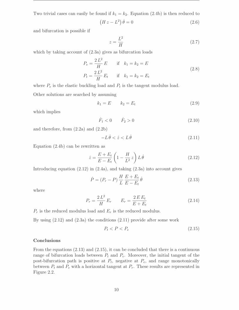
Conclusions

From the equations (2.13) and (2.15), it can be concluded that there is a continuousrange of bifurcation loads between Pt and Pe. Moreover, the initial tangent of thepost-bifurcation path is positive at Pt, negative at Pe, and range monotonicallybetween Pt and Pe with a horizontal tangent at Pr. These results are represented inFigure 2.2.

10

θ

P

Pe

Pr

Pt

Figure 2.2: Linearised analysis of Shanley’s column.

Three remarks concerning the study of this model should be mentioned [87]:

• The infinite number of bifurcations does not come from the non-linearity of thestress–strain relation but from the irreversible character of the process: a strainconfiguration can correspond to an infinite number of stress configurations,corresponding to different histories of the loading.

• The stability aspect will be studied in details in the following sections. How-ever, it can be inferred intuitively that the fundamental path will be stable ina dynamical sense up to Pr (upward tangent) and unstable after (downwardtangent).

• The conditions (2.10) assume that both springs are plasticised (k1 = k2 = Et)before the load reaches Pt. If PY is the yield limit of the springs and if Pt < PY ,then the bifurcations between Pt and PY do not exist.

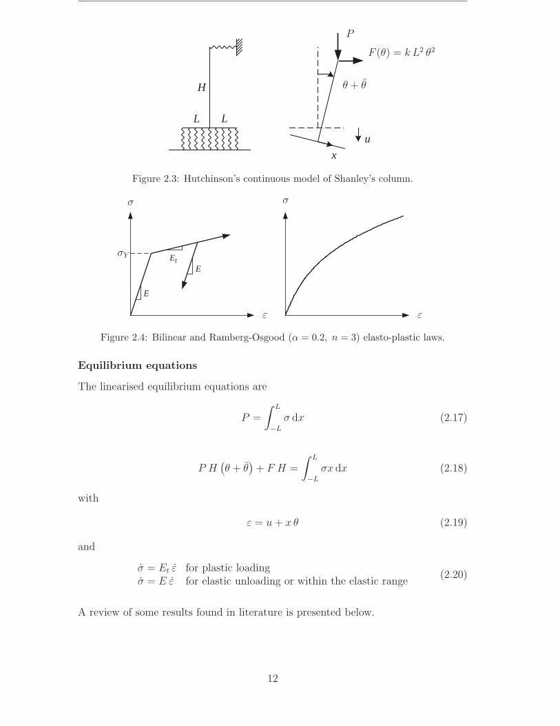
2.1.2 Hutchinson’s model

The model introduced by Hutchinson [48–50] and shown in Figure 2.3 differs fromthe previous one in that the ⊥ frame is supported by a continuous distribution ofsprings. Imperfections are represented by an initial rotation θ from the vertical in theunloaded state. Linearised analysis is performed once again and geometrical non-linearities are artificially introduced through a horizontal non-linear spring whichdevelops a force F (θ) = k L2 θ2 (k > 0).

This model has been studied with two different elasto-plastic laws as shown inFigure 2.4. The first law is the classical bilinear one while the second is of Ramberg-Osgood type defined by the equation

ε

εY

=σ

σY

+ α

(σ

σY

)n

(2.16)

11

L L

H

u

x

F (θ) = k L2 θ2

θ + θ

P

Figure 2.3: Hutchinson’s continuous model of Shanley’s column.

E

tEE

σσ

εε

σY

Figure 2.4: Bilinear and Ramberg-Osgood (α = 0.2, n = 3) elasto-plastic laws.

Equilibrium equations

The linearised equilibrium equations are

P =

∫ L

−L

σ dx (2.17)

P H(θ + θ

)+ F H =

∫ L

−L

σx dx (2.18)

with

ε = u + x θ (2.19)

and

σ = Et ε for plastic loadingσ = E ε for elastic unloading or within the elastic range

(2.20)

A review of some results found in literature is presented below.

12

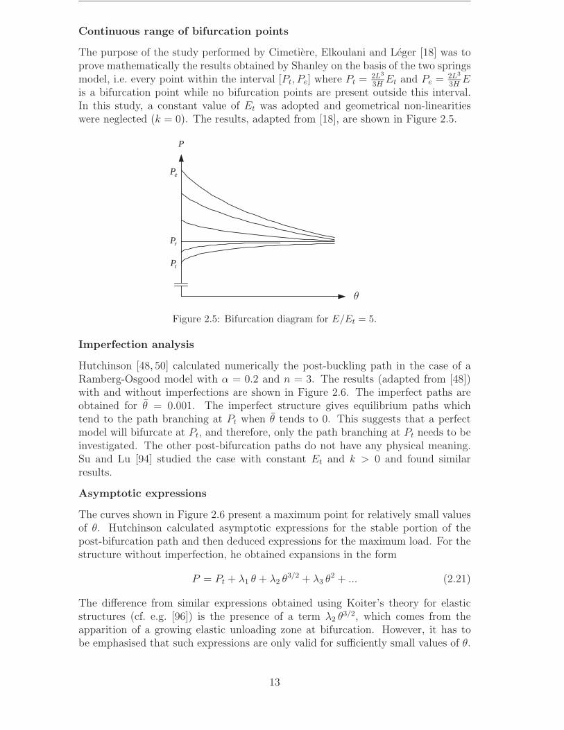
Continuous range of bifurcation points

The purpose of the study performed by Cimetiere, Elkoulani and Leger [18] was toprove mathematically the results obtained by Shanley on the basis of the two springsmodel, i.e. every point within the interval [Pt, Pe] where Pt = 2L3

3HEt and Pe = 2L3

3HE

is a bifurcation point while no bifurcation points are present outside this interval.In this study, a constant value of Et was adopted and geometrical non-linearitieswere neglected (k = 0). The results, adapted from [18], are shown in Figure 2.5.

eP

tP

P

rP

θ

Figure 2.5: Bifurcation diagram for E/Et = 5.

Imperfection analysis

Hutchinson [48, 50] calculated numerically the post-buckling path in the case of aRamberg-Osgood model with α = 0.2 and n = 3. The results (adapted from [48])with and without imperfections are shown in Figure 2.6. The imperfect paths areobtained for θ = 0.001. The imperfect structure gives equilibrium paths whichtend to the path branching at Pt when θ tends to 0. This suggests that a perfectmodel will bifurcate at Pt, and therefore, only the path branching at Pt needs to beinvestigated. The other post-bifurcation paths do not have any physical meaning.Su and Lu [94] studied the case with constant Et and k > 0 and found similarresults.

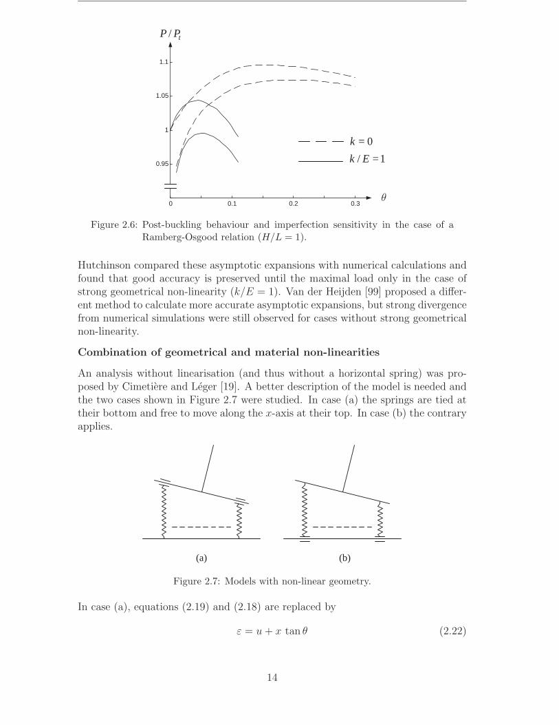
Asymptotic expressions

The curves shown in Figure 2.6 present a maximum point for relatively small valuesof θ. Hutchinson calculated asymptotic expressions for the stable portion of thepost-bifurcation path and then deduced expressions for the maximum load. For thestructure without imperfection, he obtained expansions in the form

P = Pt + λ1 θ + λ2 θ3/2 + λ3 θ2 + ... (2.21)

The difference from similar expressions obtained using Koiter’s theory for elasticstructures (cf. e.g. [96]) is the presence of a term λ2 θ3/2, which comes from theapparition of a growing elastic unloading zone at bifurcation. However, it has tobe emphasised that such expressions are only valid for sufficiently small values of θ.

13

0 0.1 0.2 0.3

0.95

1

1.05

1.1

tPP /

0=k

1/ =Ek

θ

Figure 2.6: Post-buckling behaviour and imperfection sensitivity in the case of aRamberg-Osgood relation (H/L = 1).

Hutchinson compared these asymptotic expansions with numerical calculations andfound that good accuracy is preserved until the maximal load only in the case ofstrong geometrical non-linearity (k/E = 1). Van der Heijden [99] proposed a differ-ent method to calculate more accurate asymptotic expansions, but strong divergencefrom numerical simulations were still observed for cases without strong geometricalnon-linearity.

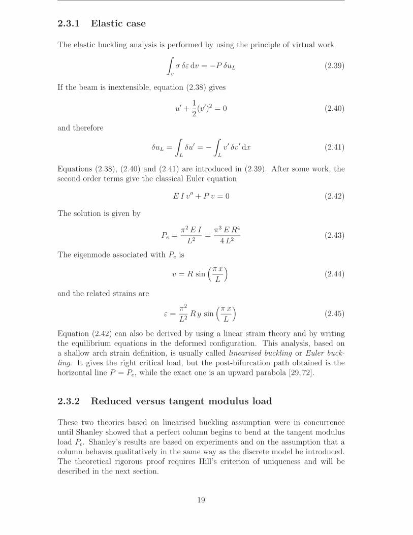
Combination of geometrical and material non-linearities

An analysis without linearisation (and thus without a horizontal spring) was pro-posed by Cimetiere and Leger [19]. A better description of the model is needed andthe two cases shown in Figure 2.7 were studied. In case (a) the springs are tied attheir bottom and free to move along the x-axis at their top. In case (b) the contraryapplies.

(a) (b)

Figure 2.7: Models with non-linear geometry.

In case (a), equations (2.19) and (2.18) are replaced by

ε = u + x tan θ (2.22)

14

P H sin θ =

∫ L

−L

σ

cos2 θx dx (2.23)

while in case (b) they are replaced by

ε = u + x sin θ (2.24)

P H sin θ =

∫ L

−L

xσ cos θ dx (2.25)

The models have been tested with a bilinear elastic-plastic law, without geometricalimperfections. The numerical results for case (a) show a monotonically increasingpost-bifurcation curve. In case (b), the bifurcated branch can be either monotoni-cally strictly increasing or it can present a maximum, depending on the ratio Et/E.

The conclusions presented in [19] are now summarised.

The cumulative effects of geometrical and material non-linearities are difficult tostudy without numerical simulations, e.g. different ratios Et/E in the bilinear elastic-plastic law or different exponents n in the Ramberg-Osgood relation can lead todifferent qualitative solutions (cf. also [61]).

With respect to the effects of material non-linearities, it can be concluded by com-paring Figures 2.5 and 2.6 that the decreasing stiffness of the material in the plasticrange (Ramberg-Osgood law) has destabilising effects.

The geometrical non-linearity can have both stabilising or destabilising effects. Thedifferences in the post-buckling paths of the cases investigated can be partly under-stood by considering only geometrical non-linearity. Four models have been studied:

• model 1 : linearised equations without geometrical imperfections

• model 2 : linearised equations with geometrical imperfections

• model 3 : non-linearised equations, case (a)

• model 4 : non-linearised equations, case (b)

The elastic post-buckling paths for these models are shown in Figure 2.8. It canbe concluded that an unstable elastic post-critical curve accentuates the possibilityof occurrence of a maximum point and a stable one accentuates the possibility of amonotonic path.

Moreover, in the vicinity of the bifurcation, material non-linearity prevails over thegeometric one and a stable path is always obtained. More detailed conclusionscannot be derived.

15

0.1

0.2

2.0 6.0

model 4

model 1

model 2

model 3

θ

P/Pc

Figure 2.8: Elastic post-buckling of the studied models.

2.2 Hill’s criterion of uniqueness

This section presents the theoretical results, due to Hill [45], concerning uniquenessof the solution of an elastic-plastic deformation.

A general solid body subjected to a quasi-static loading defined by the parameter λ isconsidered. The general boundary-value problem in elastic-plastic deformation canbe defined as follow: at a generic stage in the loading process, the current shape ofthe body and the internal stress distribution are supposed to have been determinedalready, together with the existing state of hardening and mechanical properties ingeneral. The incremental changes in all these variables have now to be calculatedfor a further infinitesimal variation λ of the loading parameter. The question of theuniqueness of the solution is then set.

The differentiation of the principle of virtual work can be written in the form∫v

Nij δuj,i dv =

∫v

bj δuj dv +

∫s

Tj δuj ds (2.26)

where Tj are the surface tractions applied on the surface s and bj are the body forces.Nij are the nominal stresses, i.e. the stresses acting in the current configuration onan infinitesimal surface element in the reference configuration. δuj is a kinematicallyadmissible virtual displacement.

Two different incremental solutions, uj and u∗j , are considered. By taking as virtual

displacement

δuj = uj − u∗j = ∆uj (2.27)

the following equation is obtained∫v

Nij (∆uj) ,i dv =

∫v

bj ∆uj dv +

∫s

Tj ∆uj ds (2.28)

16

Equation (2.28) must hold also if uj and u∗j are interchanged, that is, if Nij, bj and

Tj are replaced by N∗ij, b∗j , and T ∗

j . Subtracting these two equalities and introducingthe notations

∆Nij = Nij − N∗ij ∆bj = bj − b∗j ∆Tj = Tj − T ∗

j (2.29)

gives ∫v

∆Nij (∆uj) ,i dv =

∫v

∆bj ∆uj dv +

∫s

∆Tj ∆uj ds (2.30)

The loading is assumed conservative, which means that Tj and bj are only dependingon λ, which further implies Tj = T ∗

j and bj = b∗j . Equation (2.30) is then reduced to

H =

∫v

∆Nij (∆uj) ,i dv = 0 (2.31)

Hence, according to Hill, uniqueness of the solution is ensured if

H =

∫v

∆Nij (∆uj) ,i dv > 0 (2.32)

for every kinematically admissible ∆uj.

2.2.1 Linear comparison solid

The criterion defined in equation (2.32) is difficult to apply in practical problems.By introducing the notion of linear comparison solid, Hill proposed a second cri-terion which is easier to handle. A fictitious solid having the same configurationand stresses under the current loading as the real one, but a different incrementalconstitutive law is considered. Namely, at each material point, the fictitious solid isassumed as incrementally linear with the constitutive relationship

Nij = CLijkl ul,k (2.33)

By using the notations in (2.27) and (2.29), the modulus CLijkl is chosen such that

∆Nij (∆uj) ,i ≥ CLijkl (∆uj) ,i (∆ul) ,k (2.34)

for every pair of incremental solutions uj and u∗j .

The following functional F is then defined

F =

∫v

CLijkl (∆uj) ,i (∆ul) ,k dv (2.35)

From (2.31) and (2.34), it can be concluded that

H ≥ F (2.36)

17

and by using (2.32), the criterion of uniqueness can be expressed as

F =

∫v

CLijkl (∆uj) ,i (∆ul) ,k dv > 0 (2.37)

for every kinematically admissible ∆uj.

The problem related to equation (2.37) lies in choosing the optimal linear comparisonsolid so that the difference between F and H is as small as possible. An example ofsuch a choice is given in Section 2.3.3.

2.3 Euler beam analysis

The purpose of this section is to present a review of the different works done on theplastic buckling of a pin-ended column based on the Bernoulli plane beam assump-tions. After presenting the elastic case and the two classical theories of the tangentand reduced modulus load, a theoretical analysis is performed, starting from Hill’scriterion of uniqueness. A post-bifurcation analysis is also presented.

The column, see Figure 2.9, has a circular cross-section. It is assumed thick enoughso that elastic buckling is prohibited, but slender enough so that beam theory canstill be applied. The model adopted is based on a shallow arch strain formulationwhich, under Bernoulli hypothesis, is defined by

ε = u′ +1

2(v′)2 − y v′′ (2.38)

where a prime denotes differentiation with respect to x.

A bilinear elastic-plastic law is considered.

P

y

x

Lu

)(xv

x

y

L

R

Figure 2.9: Simply supported column with circular cross-section.

18

2.3.1 Elastic case

The elastic buckling analysis is performed by using the principle of virtual work∫v

σ δε dv = −P δuL (2.39)

If the beam is inextensible, equation (2.38) gives

u′ +1

2(v′)2 = 0 (2.40)

and therefore

δuL =

∫L

δu′ = −∫

L

v′ δv′ dx (2.41)

Equations (2.38), (2.40) and (2.41) are introduced in (2.39). After some work, thesecond order terms give the classical Euler equation

E I v′′ + P v = 0 (2.42)

The solution is given by

Pe =π2 E I

L2=

π3 E R4

4 L2(2.43)

The eigenmode associated with Pe is

v = R sin(π x

L

)(2.44)

and the related strains are

ε =π2

L2R y sin

(π x

L

)(2.45)

Equation (2.42) can also be derived by using a linear strain theory and by writingthe equilibrium equations in the deformed configuration. This analysis, based ona shallow arch strain definition, is usually called linearised buckling or Euler buck-ling. It gives the right critical load, but the post-bifurcation path obtained is thehorizontal line P = Pe, while the exact one is an upward parabola [29,72].

2.3.2 Reduced versus tangent modulus load

These two theories based on linearised buckling assumption were in concurrenceuntil Shanley showed that a perfect column begins to bend at the tangent modulusload Pt. Shanley’s results are based on experiments and on the assumption that acolumn behaves qualitatively in the same way as the discrete model he introduced.The theoretical rigorous proof requires Hill’s criterion of uniqueness and will bedescribed in the next section.

19

Apart from the historical aspect, the interest in presenting these two theories lies inthe physical description of the buckling phenomenon. Moreover, although the theoryof the reduced modulus load Pr is not correct, this load corresponds to the limitof stability along the fundamental path and has therefore a theoretical importance(cf. Section 2.4.3)

In order to simplify the calculations, a column with a rectangular cross-section(A = b h) is considered.

Reduced modulus load

It is assumed that the column remains straight while the axial load is increasedbeyond the yield point, after which the column bends, or tries to bend, at a con-stant compressive force. The problem is then the same as for Euler’s theory, i.e. todetermine deformed configurations which are in equilibrium. The calculations basedon Figure 2.10 are summarised below.

h

stresses

strains

before buckling during buckling

z

loading unloading

∆σ1 ∆σ2

∆ε

PrPr

Figure 2.10: Reduced modulus load assumptions.

∆σ1 = Et ∆ε in the loading area∆σ2 = E ∆ε in the unloading area

(2.46)

Buckling occurs at a constant axial load, which implies∫A

∆σ = 0 (2.47)

Equation (2.47) gives the position of the z axis as function of the moduli E and Et.The bending moment is then calculated according to

M =

∫A

z ∆σ (2.48)

20

which gives

M = Er I/ρ (2.49)

with

Er =

[1

2

(E−1/2 + E

−1/2t

)]−2

(2.50)

Er is called the reduced modulus and depends on the shape of the cross-section.

By introducing the classical equations

M = −P y 1/ρ = y′′ (2.51)

the following differential equation is obtained

Er I y′′ + P y = 0 (2.52)

By similarity with Euler equation, the solution is given by

Pcr = Pr =π2

L2Er I (2.53)

This result is valid under the assumption that the column is plasticised at Pr, i.e. ifPr > AσY (σY is yield limit defined in Figure 2.4).

Tangent modulus load

Actually, the column is free to bend at any time. There is nothing to prevent itfrom bending simultaneously with increasing axial load. The tangent modulus loadtheory assumes that the column remains straight until the critical load Pt is reachedand that an infinitesimal lateral deflection occurs when applying an infinitesimalincrement load ∆P in such a way that the tensile strain caused by the deflectionis compensated by the axial shortening due to ∆P . Then there is no unloadingpoint in the cross-section (cf. Figure 2.11) and ∆σ = Et ∆ε still applies everywhere.The analysis is therefore the same as in the elastic case by replacing E by Et. Thesolution (Euler) is

Pt + ∆P =π2

L2Et I (2.54)

If ∆P is assumed infinitesimal, the critical load is obtained as

Pcr = Pt =π2

L2Et I (2.55)

This result assumes also that the column is plasticised at Pt, i.e. Pt > AσY .

Remark

This approach presents a paradox. There is no elastic unloading and Et applieseverywhere. Therefore, according to Euler’s theory of buckling, the load cannot

21

h

stresses

strains

before buckling during buckling

Pt + ∆P∆σ

∆ε

Pt

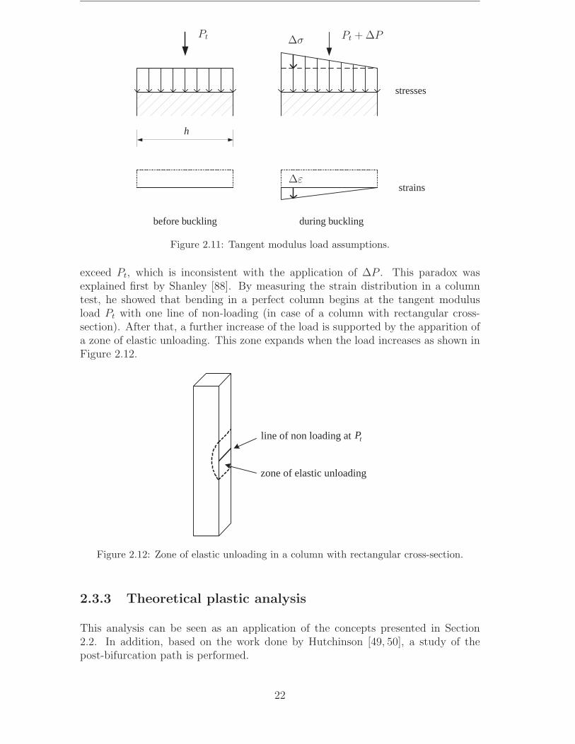
Figure 2.11: Tangent modulus load assumptions.

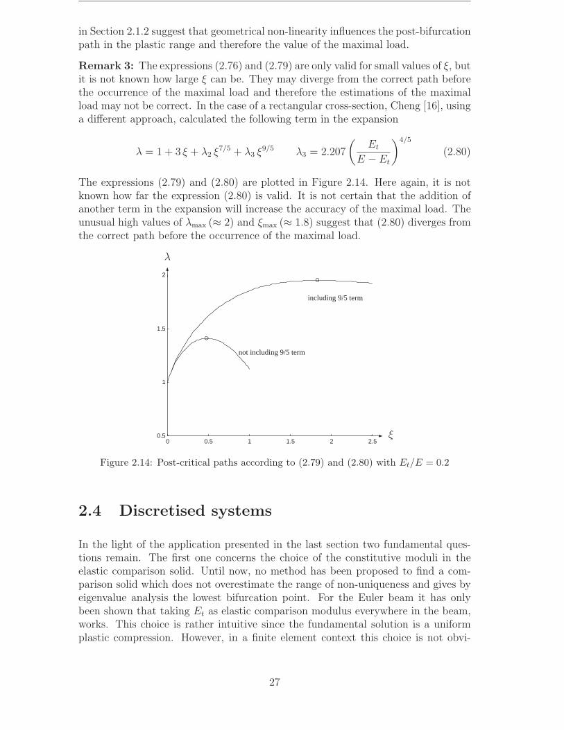
exceed Pt, which is inconsistent with the application of ∆P . This paradox wasexplained first by Shanley [88]. By measuring the strain distribution in a columntest, he showed that bending in a perfect column begins at the tangent modulusload Pt with one line of non-loading (in case of a column with rectangular cross-section). After that, a further increase of the load is supported by the apparition ofa zone of elastic unloading. This zone expands when the load increases as shown inFigure 2.12.

line of non loading at

zone of elastic unloading

tP

Figure 2.12: Zone of elastic unloading in a column with rectangular cross-section.

2.3.3 Theoretical plastic analysis

This analysis can be seen as an application of the concepts presented in Section2.2. In addition, based on the work done by Hutchinson [49, 50], a study of thepost-bifurcation path is performed.

22

The beam is assumed uniformly compressed beyond the plastic limit (P > σY π R2).The problem is to determine whether it is possible to obtain a bifurcation whenan infinitesimal load increment ∆P is applied. The incremental changes of thefundamental solution are denoted by ∆σf and ∆εf while those of the bifurcatedsolution are denoted by ∆σb and ∆εb with ε defined according to equation (2.38).

The difference between these two solutions is denoted by

∆ε = ∆εb − ∆εf ∆σ = ∆σb − ∆σf (2.56)

The function H, defined in (2.31), can be rewritten as

H =

∫v

∆σ ∆ε dv (2.57)

At P the whole beam is plasticised since the fundamental path is a pure axialcompression. The linear comparison operator CL

ijkl defined in Section 2.2 is taken as

CLijkl = Et

Hence, the function F (2.35) can be rewritten as

F =

∫v

Et ∆ε2 dv (2.58)

For this particular problem, the relation F ≤ H (2.36) can easily be proved as follow

H − F =

∫v

T dv (2.59)

with

T = (∆σ − Et ∆ε) ∆ε (2.60)

= [(∆σb − ∆σf ) − Et (∆εb − ∆εf )] (∆εb − ∆εf )

Depending on the sign of ∆εb and ∆εf , T can take the following values

• ∆εb ≤ 0 ∆εf ≤ 0 → ∆σb = Et ∆εb ∆σf = Et ∆εf

→ T = 0

• ∆εb ≤ 0 ∆εf ≥ 0 → ∆σb = Et ∆εb ∆σf = E ∆εf

→ T = (Et − E) ∆εf (∆εb − ∆εf ) ≥ 0 (Et < E)

• ∆εb ≥ 0 ∆εf ≥ 0 → ∆σb = E ∆εb ∆σf = E ∆εf

→ T = (E − Et) (∆εb − ∆εf )2 ≥ 0

• ∆εb ≥ 0 ∆εf ≤ 0 → ∆σb = E ∆εb ∆σf = Et ∆εf

→ T = (E − Et) (∆εb − ∆εf ) ∆εb ≥ 0

23

This shows that T ≥ 0 always applies and therefore H − F ≥ 0.

Bifurcation load

Let Pc be the lowest value for which the condition F = 0 is satisfied. The solutionof the variational principle δF = 0 is given in Section 2.3.1. The only modificationrequired is the replacement of E by Et. Hence, the critical load is

Pc =π2 Et I

L2=

π3 Et R4

4 L2= Pt (2.61)

and the associated eigenmode is defined by

(1)v = R sin

(π x

L

)(1)ε =

π2

L2R y sin

(π x

L

)(2.62)

Equation (2.61) confirms that the lowest bifurcation occurs at the tangent modulusload Pt as it was originally shown by Shanley.

Initial tangent

A bifurcated solution is searched as a linear combination of the fundamental pathand the eigenmode of the elastic comparison solid

∆εb − ∆εf = ξ(1)ε (2.63)

with ξ denoting the amplitude of the eigenmode defined by (2.62) which is taken asthe independent variable in the post-buckling expansion. With (2.63) F = 0, butnot H, unless both ∆εb and ∆εf have the property that no elastic unloading occursat any point in the column. The load ratio λ and its incremental variation ∆λ areintroduced as

λ =P

Pc

(2.64)

∆λ = λ − λc = λ1 ξ (λc = 1) (2.65)

If λ1 has to represent the initial tangent to the bifurcated path, a differential formof equations (2.63) and (2.65) can be obtained by the following transformations

∆εb

ξ− ∆εf

ξ=

(1)ε

∆λ

ξ= λ1 (2.66)

When ξ → 0, equations (2.66) give

εb =

εf +

(1)ε = λ1

′εf +

(1)ε (2.67)

with

() =

∂ ()

∂ξ

′() =

∂ ()

∂λ

∣∣∣∣λc

(2.68)

24

For the column

εf =σf

Et

=−λPc

π R2 Et

→ ′εf =

−π2 R2

4 L2(2.69)

Equations (2.67) and (2.69) give

εb =

π2 R2

L2

[−λ1

4+

y

Rsin(π x

L

)](2.70)

By taking λ1 large enough it is obviously possible to obtain

εb < 0 (2.71)

everywhere in the column so that no elastic unloading occurs, which further impliesH = 0. The problem is to determine which value(s) of λ1 can be solution to theboundary-value problem. For this purpose, the slope for the elastic comparison solidat bifurcation is denoted by λhe

1 . Euler analysis gives λhe1 = 0. Then λhe

1 is such that

−λhe1

4+

y

Rsin(π x

L

)> 0 (2.72)

in some part of the column and therefore1

λhe1 < λ1 (2.73)

It can then be inferred that the initial slope of the elastic-plastic solid λ1 must be thesmallest value consistent with (2.71). The reason for this is that if λ1 were larger,

then by continuity there would be some range of positive ξ whereεb would be lower

than zero everywhere. Consequently, the behaviour of the elastic-plastic solid wouldinitially coincide with that of the comparison solid so that λhe

1 = λ1. However, thispossibility is contradicted by (2.73) which implies that λ1 is the smallest value suchthat

∀x ∈ [0; L] and y ∈ [−R; R]εb =

π2 R2

L2

[−λ1

4+

y

Rsin(π x

L

)]≤ 0 (2.74)

The solution is then

λ1 = 4 (2.75)

and one point of non-loading (εb= 0) is obtained at x = L/2 and y = R. This

argumentation proves that a zone of elastic unloading spreads from this point afterthe bifurcation.

Post-bifurcation path

By performing a perturbation expansion of λ about the bifurcation point, Hutchin-son calculated an expression for the post-bifurcation path under the form

λ = 1 + 4 ξ + λ2 ξ1+β (2.76)

1The inequality (2.73) is verified in most of the common elastic-plastic problems.

25

This approach is similar to that developed in Section 2.1.2 for the ⊥ model. Here,λ2 and β are determined by an approximation of the lowest order non-vanishingterms in the equation of virtual work (2.39), which gives

λ2 = −6.337

(Et

E − Et

)1/3

β =1

3(2.77)

The analysis which leads to the above expression is rather lengthy and will not bedescribed here. It can be noted that Hutchinson showed that the second term ofthe perturbation expansion comes essentially from the apparition and expansion ofthe zone of elastic unloading. The same result was also obtained using a differentmethod by Leger and Potier-Ferry [58]. Using the expression (2.76), an estimationof the maximal load can be calculated as

λmax = 1 + 0.106E − Et

Et

ξmax = 0.106E − Et

Et

(2.78)

In the case of a rectangular cross-section, the same analysis leads to

λ = 1 + 3 ξ + λ2 ξ7/5 λ2 = −5.003

(Et

E − Et

)2/5

(2.79)

Remark 1: Contrary to the elastic case, the post-buckling path in the plastic rangedepends on the geometry of the cross-section. It comes from the growth of the elasticunloading zone which depends on the shape of the cross-section (cf. Figure 2.13).

A Asection A-A

Figure 2.13: Zone of elastic unloading for circular and rectangular cross-sections.

According to the author’s opinion, the two following remarks about expressions (2.76)and (2.79) can be stated.

Remark 2: The strain assumption (2.38) is to crude to represent correctly theelastic post-bifurcation. This study is therefore based on the assumption that inthe vicinity of the post-bifurcation path material non-linearity prevails over thegeometrical one. However it is not known how far this assumption is valid andespecially if it is still valid when the maximal load is reached. The results presented

26

in Section 2.1.2 suggest that geometrical non-linearity influences the post-bifurcationpath in the plastic range and therefore the value of the maximal load.

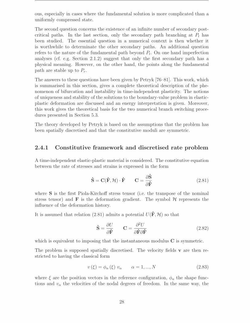
Remark 3: The expressions (2.76) and (2.79) are only valid for small values of ξ, butit is not known how large ξ can be. They may diverge from the correct path beforethe occurrence of the maximal load and therefore the estimations of the maximalload may not be correct. In the case of a rectangular cross-section, Cheng [16], usinga different approach, calculated the following term in the expansion

λ = 1 + 3 ξ + λ2 ξ7/5 + λ3 ξ9/5 λ3 = 2.207

(Et

E − Et

)4/5

(2.80)

The expressions (2.79) and (2.80) are plotted in Figure 2.14. Here again, it is notknown how far the expression (2.80) is valid. It is not certain that the addition ofanother term in the expansion will increase the accuracy of the maximal load. Theunusual high values of λmax (≈ 2) and ξmax (≈ 1.8) suggest that (2.80) diverges fromthe correct path before the occurrence of the maximal load.

0 0.5 1 1.5 20.5

1

1.5

2

including 9/5 term

not including 9/5 term

2.5

λ

ξ

Figure 2.14: Post-critical paths according to (2.79) and (2.80) with Et/E = 0.2

2.4 Discretised systems

In the light of the application presented in the last section two fundamental ques-tions remain. The first one concerns the choice of the constitutive moduli in theelastic comparison solid. Until now, no method has been proposed to find a com-parison solid which does not overestimate the range of non-uniqueness and gives byeigenvalue analysis the lowest bifurcation point. For the Euler beam it has onlybeen shown that taking Et as elastic comparison modulus everywhere in the beam,works. This choice is rather intuitive since the fundamental solution is a uniformplastic compression. However, in a finite element context this choice is not obvi-

27

ous, especially in cases where the fundamental solution is more complicated than auniformly compressed state.

The second question concerns the existence of an infinite number of secondary post-critical paths. In the last section, only the secondary path branching at Pt hasbeen studied. The essential question in a numerical context is then whether itis worthwhile to determinate the other secondary paths. An additional questionrefers to the nature of the fundamental path beyond Pt. On one hand imperfectionanalyses (cf. e.g. Section 2.1.2) suggest that only the first secondary path has aphysical meaning. However, on the other hand, the points along the fundamentalpath are stable up to Pr.

The answers to these questions have been given by Petryk [76–81]. This work, whichis summarised in this section, gives a complete theoretical description of the phe-nomenon of bifurcation and instability in time-independent plasticity. The notionsof uniqueness and stability of the solutions to the boundary-value problem in elastic-plastic deformation are discussed and an energy interpretation is given. Moreover,this work gives the theoretical basis for the two numerical branch switching proce-dures presented in Section 5.3.

The theory developed by Petryk is based on the assumptions that the problem hasbeen spatially discretised and that the constitutive moduli are symmetric.

2.4.1 Constitutive framework and discretised rate problem

A time-independent elastic-plastic material is considered. The constitutive equationbetween the rate of stresses and strains is expressed in the form

S = C(F,H) · F C =∂S

∂F(2.81)

where S is the first Piola-Kirchoff stress tensor (i.e. the transpose of the nominalstress tensor) and F is the deformation gradient. The symbol H represents theinfluence of the deformation history.

It is assumed that relation (2.81) admits a potential U(F,H) so that

S =∂U

∂FC =

∂2U

∂F∂F(2.82)

which is equivalent to imposing that the instantaneous modulus C is symmetric.

The problem is supposed spatially discretised. The velocity fields v are then re-stricted to having the classical form

v (ξ) = φα (ξ) vα α = 1, ..., N (2.83)

where ξ are the position vectors in the reference configuration, φα the shape func-tions and vα the velocities of the nodal degrees of freedom. In the same way, the

28

displacements u and the velocity variations w are given by

u (ξ) = φα (ξ) uα α = 1, ..., Nw (ξ) = φα (ξ) wα α = 1, ..., N

(2.84)

The numeration of the shape functions is chosen such that the boundary conditionsgive prescribed values vα = vα and wα = 0 for α = M + 1, ..., N .

By assuming a conservative loading, components of the prescribed load vector aregiven, in the rate form, by

Pα =

∫v

bφα dv +

∫s

Tφα ds α = 1, ...,M (2.85)

and the rates of the internal forces are given by

Qα (v) =

∫v

S (∇v) · ∇φα dv α = 1, ..., N (2.86)

where a tilde over a symbol denotes a spatial field defined over the body volume inthe reference configuration.

The equilibrium equations of the first order problem in velocities are

Qα (v) = Pα α = 1, ...,M (2.87)

The components of the tangent stiffness matrix are defined by

Kαβ (v) =∂Qα (v)

∂vβ

=

∫v

∇φα · C (∇v) · ∇φβ dv (2.88)

which allows the reformulation of the equilibrium equations (2.87) as

Kαβ (v) vβ = Pα α = 1, ...,M (2.89)

From (2.82) and (2.88), it follows that K is symmetric, i.e. Kαβ = Kβα.

Since the existence of a potential U is assumed, a functional J can be defined as

J (v) =

∫v

U (∇v) dv −M∑

α=1

Pα vα =1

2Kαβ (v) vβ vα −

M∑α=1

Pα vα (2.90)

The equations (2.87) or (2.89) can then be given the variational formulation

∂J (v)

∂vα

= 0 α = 1, ...,M (2.91)

From (2.90), the tangent stiffness matrix can also be expressed as

Kαβ (v) =∂2J (v)

∂vα ∂vβ

(2.92)

29

2.4.2 Tangent comparison solid

The theory developed by Hill (cf. Section 2.2) does not require any solution to beknown in advance. However, in practice a fundamental solution is known and the op-timal choice for the linear comparison solid can be determined from the fundamentalsolution, as explained in the following.

The elastic operator is Ceijkl. Where the yield condition is satisfied, the elasto-plastic

operator is Ceijkl in case of elastic unloading, and Cp

ijkl in case of plastic loading. The

linear comparison operator CLijkl is defined by

CLijkl = Cp

ijkl (2.93)

at every point in the body where the yield condition is currently satisfied, indepen-dent of the case (plastic loading or elastic unloading) concerned, and by

CLijkl = Ce

ijkl (2.94)

at every point where the stresses lie within the yield surface. With this choice, itcan be proved that the condition (2.34) is respected for elastic-plastic material withsmooth yield surface.

In other words, the actual tangent moduli of the fundamental solution is taken aslinear comparison solid. For this reason Petryk introduced the notion of tangentcomparison solid.

It can be noted that in the analysis of Euler beam in Section 2.3.3, CLijkl = Et has

been assumed, which actually corresponds to the tangent comparison solid.

2.4.3 Bifurcation and stability

Directional stability of an equilibrium state

The notion of stability is often referred to the definition given by Liapunov. Roughlyspeaking, an equilibrium state is stable if after applying a small perturbation atconstant loading, the damped structure returns to the previous equilibrium state.For elastic-plastic structures, this cannot be expected in general. Moreover, evenif the equilibrium state after perturbation is very close to the original one, there isno guarantee that the continuation of the loading process will not give divergencebetween the two paths. To avoid this problem, Petryk proposed a different definitionof stability of an equilibrium state: “an equilibrium configuration is said to bestable if the distance from that configuration in any dynamic motion caused by adisturbance can be made as small as we please if a measure of the disturbance itselfis sufficiently small.” He introduced a restriction to this definition by consideringthat the perturbed motion from the equilibrium state is such that variations of thedirection of the velocity field is negligible. In that restrictive sense, he introducedthe notion of directional stability.

30

Under these assumptions, it can be proved that an equilibrium state is directionallystable if

Qα (w) wα > 0 for every w = 0 (2.95)

Uniqueness of the solution

It is supposed that a fundamental solution vf to the equation (2.87) is known. Therespective tangent stiffness matrix is denoted Kf . Petryk has shown that if thecondition (2.95) is respected, uniqueness of the solution is ensured if vf assigns toJ a strict and absolute minimum value, i.e. if

J (vf ) < J (v) for every admissible v (2.96)

By using equations (2.91) and (2.92) and the condition (2.96), it can be concludedthat uniqueness of the solution is ensured as long as Kf is positive definite. Thisresult can also be obtained from Hill’s criterion of uniqueness. The definition ofthe tangent comparison solid allows to use results for elastic structures. Thereforeequation (2.37) ensures uniqueness of the solution as long as Kf is positive definite.

This criterion holds for elastic-plastic materials obeying the normality flow rulerelative to a smooth yield surface. This is the case for the von Mises materialwhich will be used in the numerical applications. Petryk proposed a less restrictivecondition

Sf · F − S · Ff ≥ 0 for every admissible F (2.97)

where S = CF. For the applications in this thesis, this condition does not need tobe further investigated.

Continuous range of bifurcation

The question investigated here is to determine what happens beyond the first bifur-cation point when the tangent stiffness matrix Kf ceases to be positive definite. Itis possible that on the secondary post-bifurcation path the tangent stiffness matrixbecomes positive definite again. This is due to the local elastic unloading whichstarts at the bifurcation (cf. e.g. the case of the Euler beam in Section 2.3). In thatcase, uniqueness of the solution is guaranteed and the secondary path can be treatedexactly in the same way as the fundamental path before bifurcation.

The situation is different on the fundamental path where Kf becomes indefiniteafter the first bifurcation point. If the condition (2.95) fails at the same point whereKf becomes indefinite then this critical point is a limit point. If the condition (2.95)is still valid beyond the first critical point, it can be shown that there is a bifurca-tion at every point on the fundamental path along which Kf is indefinite and thecondition (2.95) holds. This defines a continuous range of bifurcation points alongthe fundamental path. It has to be noted that every point within this interval isstable in a dynamical sense. These results, illustrated in Figure 2.15, can be seenas a generalisation of the results obtained for Shanley’s column, i.e., along the fun-damental path every point within the interval [Pt, Pr] is a bifurcation point and isstable in the dynamical sense.

31

fK

positive definiteuniqueness

continuous range ofbifurcations

directional instability

deviation from thefundamental path

λ

Qα wα > 0

Figure 2.15: Schematic illustration of the results of Section 2.4.3.

2.4.4 Energy approach

Instability of a deformation path

The case of a continuous range of bifurcation points is considered. The questioninvestigated here is to determine among all these possible paths which ones arerealisable in a physical sense. The response can be found by introducing small im-perfections: when the imperfections tend to zero, the equilibrium paths obtainedtend to the secondary path branching out at the lowest bifurcation point. Thisproves that only this secondary path has a physical meaning. A probabilistic ap-proach gives the same result: if at a bifurcation point both paths (fundamental andsecondary) have comparable chances to be followed, then, due to the infinite numberof bifurcation points, any segment of the fundamental path has zero probability tobe followed. Therefore it can be concluded that beyond the first bifurcation point,the fundamental path, even if each equilibrium point along it is stable in a dynam-ical sense, has no physical meaning and can be considered as unstable. The notionof stability introduced here does not concern any more an equilibrium point but adeformation path: a deformation path is said to be unstable if it cannot be followedin a physical sense.

Energy interpretation

The purpose of this section is to give an energy interpretation of the notion ofinstability of a deformation path.

The deformation work in the body during a deformation process is expressed as

W =

∫ t

0

Qα vα dτ (2.98)

32

The potential energy of the loading is expressed as

Ω = −M∑

α=1

Pα uα (2.99)

The energy functional is then defined by

E = W + Ω (2.100)

An increment of the value of E can be interpreted as the amount of external energywhich has to be supplied to the system consisting of the body and the loading inorder to produce the deformation increment.

By time derivation, it can be shown that E is independent of v, i.e.

E (v) = constant (2.101)

and that if v1 and v2 are two admissible velocity fields at the equilibrium state

1

2E (v1) − 1

2E (v2) = J (v1) − J (v2) (2.102)

where J is the functional defined in equation (2.90). Hence, the variational princi-ple (2.91) can be equivalently written as

δE (v, w) = 0 for every admissible w = 0 (2.103)

The following criterion of path instability is then adopted: along a stable deforma-tion path, the deformation increment must minimise the value of the increment ofthe energy functional E. This can be related to the physical hypothesis that the realdeformation path minimises the energy consumption. By using (2.101), the solutionv1 is therefore stable in an energy sense if

E (v1) < E (v) for every admissible v (2.104)

which, from (2.102) can be rewritten as

J (v1) < J (v) for every admissible v (2.105)

By comparing (2.96) and (2.105) it can be concluded that the fundamental solutionvf is stable as long as the uniqueness of the solution is guaranteed. Beyond the firstbifurcation point the tangent matrix Kf becomes indefinite along the fundamentalpath. Therefore, from (2.92), the fundamental solution vf does no longer minimiseE and the solution becomes unstable in the energy sense. It can be proved thatanother solution which minimises E exists as long as the condition (2.95) holds.

As a conclusion, it has been shown that the definition of stability in an energy sense(minimisation of the consumption of energy) proposed by Petryk is equivalent to thenotion of stability of a deformation path given in the previous section. Consequently,the fundamental path vf becomes unstable exactly when the tangent stiffness matrixKf becomes indefinite.

33

Chapter 3

2D beam element formulation

In this chapter, internal forces and tangent stiffness matrices for three plane beamelements are derived. All of them are based on the same co-rotational approach,and differ by the strain definition used in the local co-rotational coordinate system.Based on the Bernoulli assumption, the first two elements use a linear and a shallowarch strain definition, respectively. The third element is based on the Timoshenkoassumption with linear interpolations for the displacements.

Co-rotational formulation

The co-rotational approach, viewed as an alternative way of deriving efficient non-linear finite elements, has generated an increased amount of interest in the lastdecade [22, 23, 25, 35, 47, 53, 64, 72, 73, 83, 84, 95]. The main idea in this context isto decompose the motion of the element into rigid body and pure deformationalparts, through the use of a local coordinate system (xl, zl), see Figure 3.1, whichcontinuously rotates and translates with the element. The motion of the elementfrom the original undeformed configuration to the actual deformed one can thus besplit in two steps. The first one is a rigid rotation and translation of the element. Thesecond step consists of a deformation in the local coordinate system. Assuming thatthe length of the element is properly chosen, the deformational part of the motion isalways small relative to the local axes. Consequently, the local deformations can beexpressed with a low order of non-linearity. It must however be emphasised that thislow-order non-linearity is only apparent as the geometrical non-linearity is includedin the motion of the local coordinate system.

The main advantage of a co-rotational approach is that it leads to an artificialseparation of the material and geometrical non-linearities when a linear strain def-inition in the local coordinate system is used (which is the case for the first andthird elements developed in this chapter): plastic deformations occur in the localcoordinate system where geometrical linearity is assumed; geometrical non-linearityis only present during the rigid rotation and translation of the undeformed beam.This leads to very simple expressions for the local internal force vector and tangentstiffness matrix. Even when a low-order geometrical non-linearity is included in thestrain definition (which is the case of the second element), the expressions for thelocal internal force vector and tangent stiffness matrix are still very simple.

35

Constitutive equations

The assumption of small strains but large displacements and rotations, is adopted.Therefore, constitutive elasto-plastic equations based on an additive strain decom-position can be used. In this thesis, a von Mises material with isotropic constanthardening is considered. The reason for this choice has already been discussed inSection 1.1. For the Timoshenko element, interaction between the normal and theshear stress is considered and the constitutive equations are derived from the onesunder plane stress conditions by introducing the beam hypothesis.

Resultant forces against Gauss integration

The computation of the local internal forces and stiffness matrix involves severalintegrations over the element. With respect to integration over a cross-section, twoapproaches can be considered: the layered and non-layered ones [67].

The non-layered method is based on plastic equations at the section level. Thismeans that the yield criterion is defined as a function of the internal forces. Suchfunctions can be found in [1,56,89] for rectangular and bi-symmetric cross-sections.However, these functions are only approximations of the plastic flow rules. More-over, they do not model the propagation of plastification and they consider perfectelasto-plastic material models without hardening. For the Bernoulli assumption,Crisfield [24] proposes a function which takes into account the propagation of theplastification, but without considering hardening. Another problem with this ap-proach is the practical impossibility to derive functions for arbitrary cross-sections.

As shown in Chapter 2 for the case of the Euler beam, a growing zone of elastic un-loading is developing after bifurcation. Furthermore, the bifurcation point and thenature of the post-bifurcation path are dependent on the hardening. It seems there-fore impossible to study plastic instability problems with a non-layered approach.This method, though efficient from a computational point of view, is limited to quickand approximate analyses.

In the layered approach, numerical Gauss integration is performed through the cross-section which means that the plastic rate equations are solved at each Gauss point.A relatively high number of Gauss points is needed in order to model correctly thegrowing of the elastic unloading zone (case of the Euler beam) and obtain an accuratepost-bifurcation path. As alternative to Gauss integration, the Lobatto rule couldalso be considered. This procedure has the advantage of taking integration pointson the surface. However, if a sufficient number of points is taken, both methods givealmost the same numerical results.

3.1 Co-rotational framework

The purpose of this section is to derive relations between the local and global ex-pressions of the internal force vector and tangent stiffness matrix. This presentationis mainly taken from Crisfield [23].

36

3.1.1 Beam kinematics

1

2

x

z

u1

u2w1

w2

u xlzl

βo

βαθ1

θ2θ1

θ2

Figure 3.1: Co-rotational formulation: beam kinematics.

The notations used in this section are defined in Figure 3.1. The coordinates for thenodes 1 and 2 in the global coordinate system (x, z) are (x1, z1) and (x2, z2). Thevector of global displacements is defined by

pg =[

u1 w1 θ1 u2 w2 θ2

]T(3.1)

The vector of local displacements is defined by

pl =[

u θ1 θ2

]T(3.2)

The components of pl can be computed according to

u = ln − lo (3.3a)

θ1 = θ1 − α (3.3b)

θ2 = θ2 − α (3.3c)

In the above equations lo and ln denote the initial and current lengths of the element

lo =[(x2 − x1)

2 + (z2 − z1)2]1/2

(3.4)

ln =[(x2 + u2 − x1 − u1)

2 + (z2 + w2 − z1 − w1)2]1/2

(3.5)

and α denotes the rigid rotation which can be computed as

sin α = co s − so c (3.6a)

cos α = co c + so s (3.6b)

37

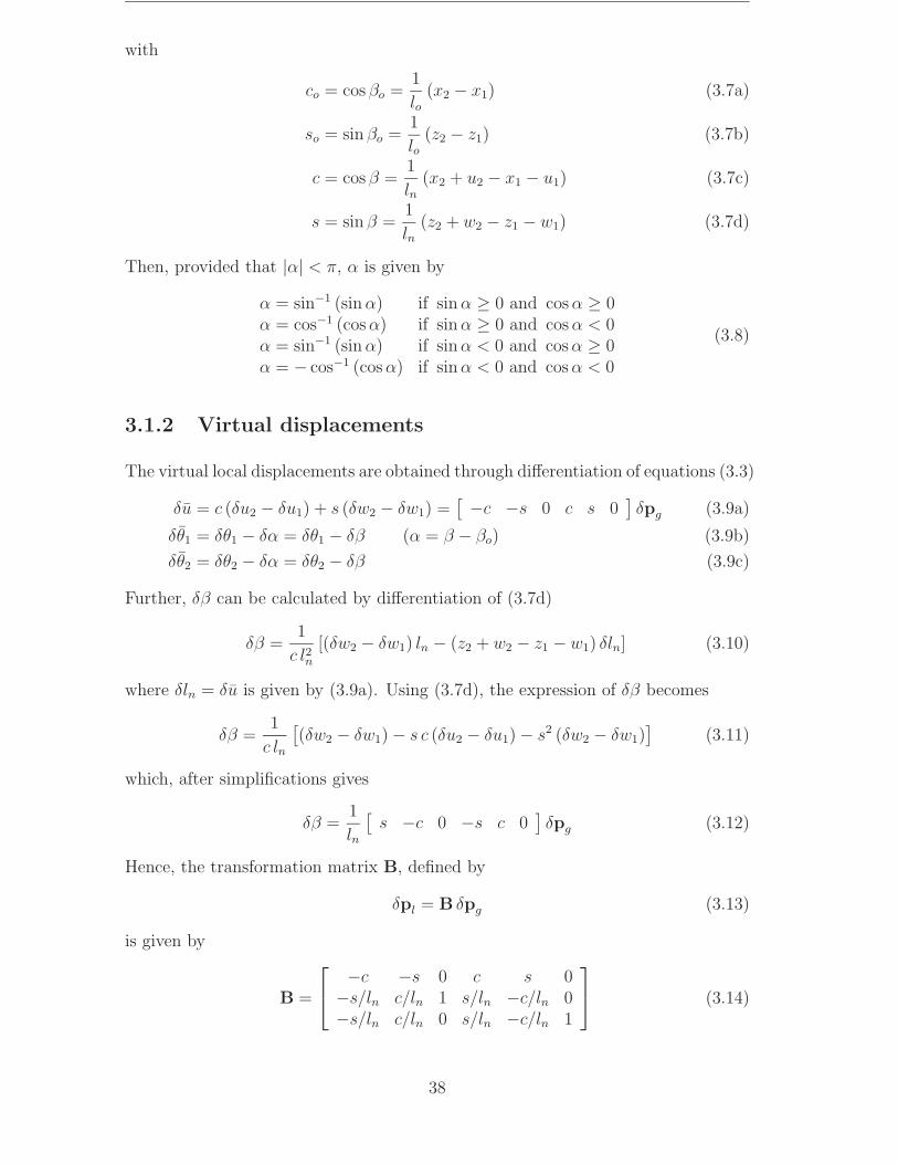
with

co = cos βo =1

lo(x2 − x1) (3.7a)

so = sin βo =1

lo(z2 − z1) (3.7b)

c = cos β =1

ln(x2 + u2 − x1 − u1) (3.7c)

s = sin β =1

ln(z2 + w2 − z1 − w1) (3.7d)

Then, provided that |α| < π, α is given by

α = sin−1 (sin α) if sin α ≥ 0 and cos α ≥ 0α = cos−1 (cos α) if sin α ≥ 0 and cos α < 0α = sin−1 (sin α) if sin α < 0 and cos α ≥ 0α = − cos−1 (cos α) if sin α < 0 and cos α < 0

(3.8)

3.1.2 Virtual displacements

The virtual local displacements are obtained through differentiation of equations (3.3)

δu = c (δu2 − δu1) + s (δw2 − δw1) =[ −c −s 0 c s 0

]δpg (3.9a)

δθ1 = δθ1 − δα = δθ1 − δβ (α = β − βo) (3.9b)

δθ2 = δθ2 − δα = δθ2 − δβ (3.9c)

Further, δβ can be calculated by differentiation of (3.7d)

δβ =1

c l2n[(δw2 − δw1) ln − (z2 + w2 − z1 − w1) δln] (3.10)

where δln = δu is given by (3.9a). Using (3.7d), the expression of δβ becomes

δβ =1

c ln

[(δw2 − δw1) − s c (δu2 − δu1) − s2 (δw2 − δw1)

](3.11)

which, after simplifications gives

δβ =1

ln

[s −c 0 −s c 0

]δpg (3.12)

Hence, the transformation matrix B, defined by

δpl = B δpg (3.13)

is given by

B =

−c −s 0 c s 0

−s/ln c/ln 1 s/ln −c/ln 0−s/ln c/ln 0 s/ln −c/ln 1

(3.14)

38

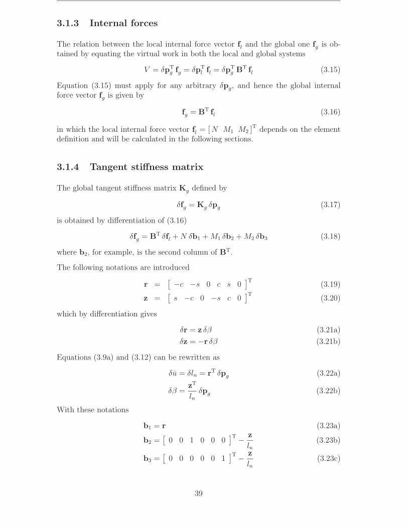
3.1.3 Internal forces

The relation between the local internal force vector fl and the global one fg is ob-tained by equating the virtual work in both the local and global systems

V = δpTg fg = δpT

l fl = δpTg BT fl (3.15)

Equation (3.15) must apply for any arbitrary δpg, and hence the global internalforce vector fg is given by

fg = BT fl (3.16)

in which the local internal force vector fl = [ N M1 M2 ]T depends on the elementdefinition and will be calculated in the following sections.

3.1.4 Tangent stiffness matrix

The global tangent stiffness matrix Kg defined by

δfg = Kg δpg (3.17)

is obtained by differentiation of (3.16)

δfg = BT δfl + N δb1 + M1 δb2 + M2 δb3 (3.18)

where b2, for example, is the second column of BT.

The following notations are introduced

r =[ −c −s 0 c s 0

]T(3.19)

z =[

s −c 0 −s c 0]T

(3.20)

which by differentiation gives

δr = z δβ (3.21a)

δz = −r δβ (3.21b)

Equations (3.9a) and (3.12) can be rewritten as

δu = δln = rT δpg (3.22a)

δβ =zT

lnδpg (3.22b)

With these notations

b1 = r (3.23a)

b2 =[

0 0 1 0 0 0]T − z

ln(3.23b)

b3 =[

0 0 0 0 0 1]T − z

ln(3.23c)

39

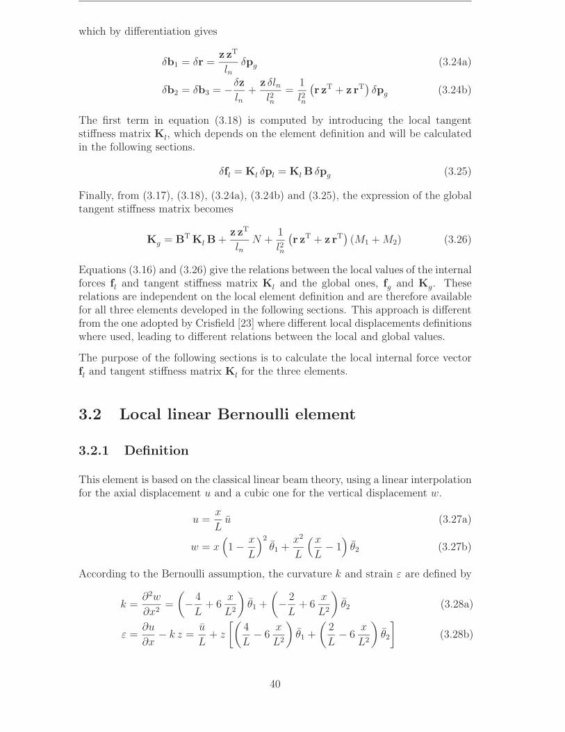
which by differentiation gives

δb1 = δr =z zT

lnδpg (3.24a)

δb2 = δb3 = −δz

ln+

z δlnl2n

=1

l2n

(r zT + z rT

)δpg (3.24b)

The first term in equation (3.18) is computed by introducing the local tangentstiffness matrix Kl, which depends on the element definition and will be calculatedin the following sections.

δfl = Kl δpl = Kl B δpg (3.25)

Finally, from (3.17), (3.18), (3.24a), (3.24b) and (3.25), the expression of the globaltangent stiffness matrix becomes

Kg = BT Kl B +z zT

lnN +

1

l2n

(r zT + z rT

)(M1 + M2) (3.26)

Equations (3.16) and (3.26) give the relations between the local values of the internalforces fl and tangent stiffness matrix Kl and the global ones, fg and Kg. Theserelations are independent on the local element definition and are therefore availablefor all three elements developed in the following sections. This approach is differentfrom the one adopted by Crisfield [23] where different local displacements definitionswhere used, leading to different relations between the local and global values.

The purpose of the following sections is to calculate the local internal force vectorfl and tangent stiffness matrix Kl for the three elements.

3.2 Local linear Bernoulli element

3.2.1 Definition

This element is based on the classical linear beam theory, using a linear interpolationfor the axial displacement u and a cubic one for the vertical displacement w.

u =x

Lu (3.27a)

w = x(1 − x

L

)2

θ1 +x2

L

(x

L− 1)

θ2 (3.27b)

According to the Bernoulli assumption, the curvature k and strain ε are defined by

k =∂2w

∂x2=

(− 4

L+ 6

x

L2

)θ1 +

(− 2

L+ 6

x

L2

)θ2 (3.28a)

ε =∂u

∂x− k z =

u

L+ z

[(4

L− 6

x

L2

)θ1 +

(2

L− 6

x

L2

)θ2

](3.28b)

40

3.2.2 Gauss integration

Because of the non-linear relation between ε and σ, it is not possible to deriveanalytical expressions for the internal forces and the local tangent stiffness matrixand a Gauss quadrature has to be adopted. The number of Gauss points per sectionhas already been discussed: two cases, with seven and fifteen points are considered.The number of sections, i.e. the number of Gauss points along the beam axis is takenas two in order to obtain the exact solution for the elastic case (the elastic strainenergy defined by Φ = 1

2

∫vEε2dv is a polynomial of second order in x and therefore

is exactly evaluated using a two points Gauss integration). Taking more points alongthe beam axis would of course increase the precision in the elasto-plastic case, butat some computational cost.

The position (and weight) of the Gauss points are within 0 < x < L

x1 =L

2

(1 − 1√

3

) (L

2

)x2 =

L

2

(1 +

1√3

) (L

2

)(3.29)

3.2.3 Local internal forces

The local internal forces are calculated by using the theorem of virtual work

V =

∫v

σ δε dv = N δu + M1 δθ1 + M2 δθ2 (3.30)

which by introducing (3.28b) gives

V =

∫v

σ

[δu

L+ z

(4

L− 6

x

L2

)δθ1 + z

(2

L− 6

x

L2

)δθ2

]dv (3.31)

Equation (3.30) must apply for every(δu, δθ1, δθ2

)and hence the local internal forces

are given by

N =

∫v

σ

Ldv (3.32a)

M1 =

∫v

σ z

(4

L− 6

x

L2

)dv (3.32b)

M2 =

∫v

σ z

(2

L− 6

x

L2

)dv (3.32c)

Using a two points Gauss integration gives

N =1

2

[∫A1

σ dA1 +

∫A2

σ dA2

](3.33a)

M1 =

√3 + 1

2

∫A1

σ z dA1 +1 −√

3

2

∫A2

σ z dA2 (3.33b)

M2 =

√3 − 1

2

∫A1

σ z dA1 −√

3 + 1

2

∫A2

σ z dA2 (3.33c)

41

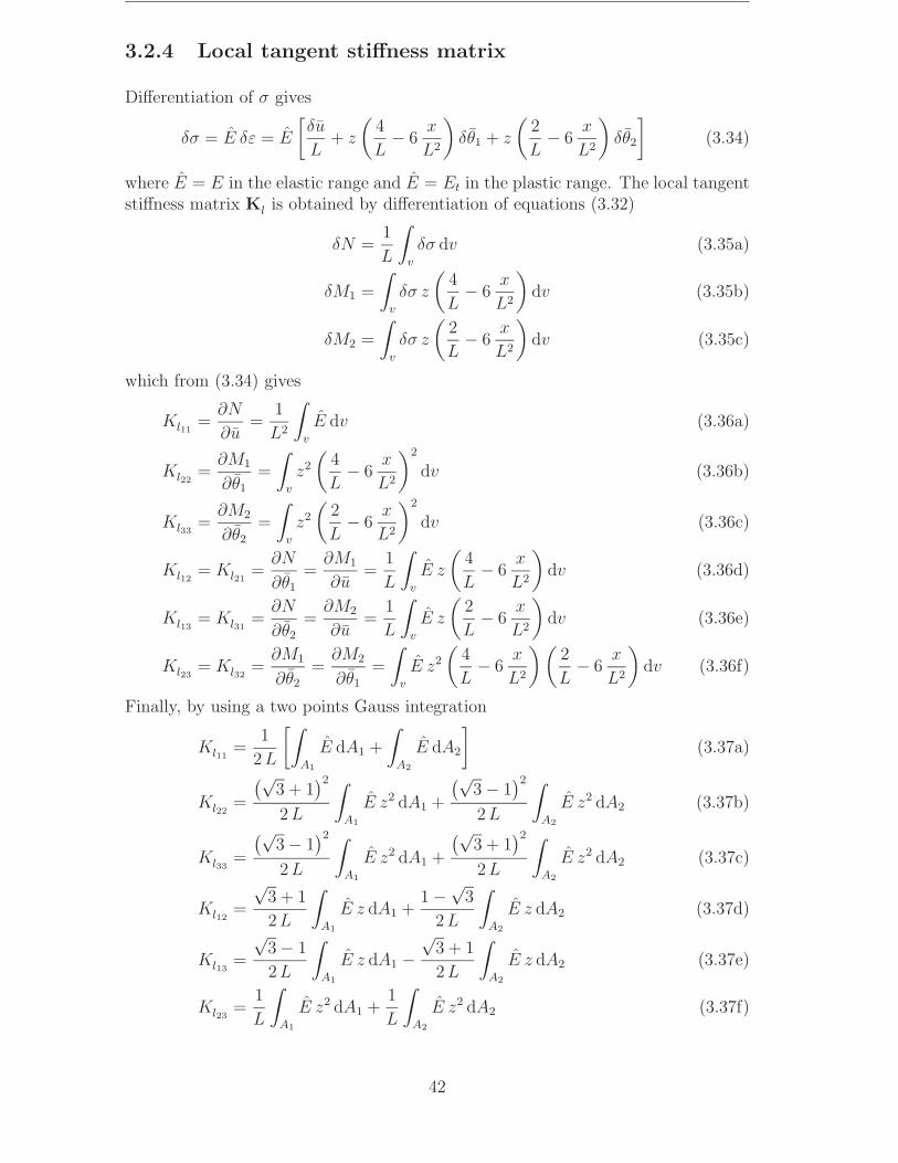
3.2.4 Local tangent stiffness matrix

Differentiation of σ gives

δσ = E δε = E

[δu

L+ z

(4

L− 6

x

L2

)δθ1 + z

(2

L− 6

x

L2

)δθ2

](3.34)

where E = E in the elastic range and E = Et in the plastic range. The local tangentstiffness matrix Kl is obtained by differentiation of equations (3.32)

δN =1

L

∫v

δσ dv (3.35a)

δM1 =

∫v

δσ z

(4

L− 6

x

L2

)dv (3.35b)

δM2 =

∫v

δσ z

(2

L− 6

x

L2

)dv (3.35c)

which from (3.34) gives

Kl11=

∂N

∂u=

1

L2

∫v

E dv (3.36a)

Kl22=

∂M1

∂θ1

=

∫v

z2

(4

L− 6

x

L2

)2

dv (3.36b)

Kl33=

∂M2

∂θ2

=

∫v

z2

(2

L− 6

x

L2

)2

dv (3.36c)

Kl12= Kl21

=∂N

∂θ1

=∂M1

∂u=

1

L

∫v

E z

(4

L− 6

x

L2

)dv (3.36d)

Kl13= Kl31

=∂N

∂θ2

=∂M2

∂u=

1

L

∫v

E z

(2

L− 6

x

L2

)dv (3.36e)

Kl23= Kl32

=∂M1

∂θ2

=∂M2

∂θ1

=

∫v

E z2

(4

L− 6

x

L2

)(2

L− 6

x

L2

)dv (3.36f)

Finally, by using a two points Gauss integration

Kl11=

1

2 L

[∫A1

E dA1 +

∫A2

E dA2

](3.37a)

Kl22=

(√3 + 1

)22 L

∫A1

E z2 dA1 +

(√3 − 1

)22 L

∫A2

E z2 dA2 (3.37b)

Kl33=

(√3 − 1

)22 L

∫A1

E z2 dA1 +

(√3 + 1

)22 L

∫A2

E z2 dA2 (3.37c)

Kl12=

√3 + 1

2 L

∫A1

E z dA1 +1 −√

3

2 L

∫A2

E z dA2 (3.37d)

Kl13=

√3 − 1

2 L

∫A1

E z dA1 −√

3 + 1

2 L

∫A2

E z dA2 (3.37e)

Kl23=

1

L

∫A1

E z2 dA1 +1

L

∫A2

E z2 dA2 (3.37f)

42

3.2.5 Constitutive equations

A bilinear strain–stress relation, see Figure 3.2, with an isotropic hardening isadopted. This model presents a constant modulus Et in the plastic range, andtherefore the influence of the decreasing of Et, cf. Section 2.1.2, cannot be studied.

σ

εεY

σY

E

EEt

Figure 3.2: Bilinear elastic-plastic law.

3.3 Local shallow arch Bernoulli element

3.3.1 Definition

The second element uses a shallow arch definition for the local strain, according to

ε = εf − k z =1

L

∫L

[∂u

∂x+

1

2

(∂w

∂x

)2]

dx − k z (3.38)

In (3.38), an averaged measure for the axial strain is introduced in order to avoidmembrane locking. Using the same definition of the curvature and the same inter-polations as in Section 3.2.1, gives

ε =u

L+

1

15θ 21 − 1

30θ1 θ2 +

1

15θ 22 + z

[(4

L− 6

x

L2

)θ1 +

(2

L− 6

x

L2

)θ2

](3.39)

For the same reason as in Section 3.2.2, a two points Gauss integration along thebeam axis is adopted.

3.3.2 Local internal forces

As before, the local internal forces are computed using the theorem of virtual work

V =

∫v

σ δε dv = N δu + M1 δθ1 + M2 δθ2 (3.40)

43

with δε evaluated from (3.39)

δε =δu

L+

2

15θ1 δθ1 − 1

30θ1 δθ2 − 1

30θ2 δθ1 +

2

15θ2 δθ2 (3.41)

+z

[(4

L− 6

x

L2

)δθ1 +

(2

L− 6

x

L2

)δθ2

]

Hence

N =

∫v

σ

Ldv (3.42a)

M1 =

(2

15θ1 − 1

30θ2

)∫v

σ dv +

∫v

σ z

(4

L− 6

x

L2

)dv (3.42b)

M2 =

(2

15θ2 − 1

30θ1

)∫v

σ dv +

∫v

σ z

(2

L− 6

x

L2

)dv (3.42c)

which, using a two points Gauss integration, gives

N =1

2

[∫A1

σ dA1 +

∫A2

σ dA2

](3.43a)

M1 =L

2

(2

15θ1 − 1

30θ2

)[∫A1

σ dA1 +

∫A2

σ dA2

]

+

√3 + 1

2

∫A1

σ z dA1 +1 −√

3

2

∫A2

σ z dA2

(3.43b)

M2 =L

2

(2

15θ2 − 1

30θ1

)[∫A1

σ dA1 +

∫A2

σ dA2

]

+

√3 − 1

2

∫A1

σ z dA1 −√

3 + 1

2

∫A2

σ z dA2

(3.43c)

3.3.3 Local tangent stiffness matrix

The local tangent stiffness matrix is calculated by differentiation of (3.42).

δN =1

L

∫v

δσ dv (3.44a)

δM1 =

(2

15δθ1 − 1

30δθ2

)∫v

σ dv +

(2

15θ1 − 1

30θ2

)∫v

δσ dv

+

∫v

δσ z

(4

L− 6

x

L2

)dv

(3.44b)

δM2 =

(2

15δθ2 − 1

30δθ1

)∫v

σ dv +

(2

15θ2 − 1

30θ1

)∫v

δσ dv

+

∫v

δσ z

(2

L− 6

x

L2

)dv

(3.44c)

with δσ = E δε and δε given in (3.41). Using a two points Gauss rule, the localtangent stiffness matrix is evaluated as

44

Kl11=

∂N

∂u=

1

2L

[∫A1

E dA1 +

∫A2

E dA2

](3.45a)

Kl12=

∂N

∂θ1

=1

2

(2

15θ1 − 1

30θ2

)[∫A1

E dA1 +

∫A2

E dA2

]

+

√3 + 1

2 L

∫A1

E z dA1 +1 −√

3

2 L

∫A2

E z dA2

(3.45b)

Kl13=

∂N

∂θ2

=1

2

(2

15θ2 − 1

30θ1

)[∫A1

E dA1 +

∫A2

E dA2

]

+

√3 − 1

2 L

∫A1

E z dA1 −√

3 + 1

2 L

∫A2

E z dA2

(3.45c)

Kl22=

∂M1

∂θ1

=1

2L

(2

15θ1 − 1

30θ2

)2 [∫A1

E dA1 +

∫A2

E dA2

]

+

(2

15θ1 − 1

30θ2

)[(√3 + 1

)∫A1

E z dA1 +(1 −

√3)∫

A2

E z dA2

]

+

(√3 + 1

)22 L

∫A1

E z2 dA1 +

(√3 − 1

)22 L

∫A2

E z2 dA2

+L

15

[∫A1

σ dA1 +

∫A2

σ dA2

](3.45d)

Kl33=

∂M2

∂θ2

=1

2L

(2

15θ2 − 1

30θ1

)2 [∫A1

E dA1 +

∫A2

E dA2

]

+

(2

15θ2 − 1

30θ1

)[(√3 − 1

)∫A1

E z dA1 −(√

3 + 1)∫

A2

E z dA2

]

+

(√3 − 1

)22 L

∫A1

E z2 dA1 +

(√3 + 1

)22 L

∫A2

E z2 dA2

+L

15

[∫A1

σ dA1 +

∫A2

σ dA2

](3.45e)

Kl23=

∂M1

∂θ2

=1

2L

(2

15θ1 − 1

30θ2

)(2

15θ2 − 1

30θ1

)[∫A1

E dA1 +

∫A2

E dA2

]

+

[√3 − 1

2

(2

15θ1 − 1

30θ2

)+

√3 + 1

2

(2

15θ2 − 1

30θ1

)]∫A1

E z dA1

−[√

3 + 1

2

(2

15θ1 − 1

30θ2

)+

√3 − 1

2

(2

15θ2 − 1

30θ1

)]∫A2

E z dA2

+1

L

[∫A1

E z2 dA1 +

∫A2

E z2 dA2

]− L

60

[∫A1

σ dA1 +

∫A2

σ dA2

](3.45f)

Kl21= Kl12

Kl31= Kl13

Kl32= Kl23

(3.45g)

45

Constitutive equations

The same elastic-plastic model as for the previous element is used.

3.4 Local linear Timoshenko element

3.4.1 Definition

A classical two noded Timoshenko beam element is defined with linear interpolationsfor u, w and θ in the local co-rotational coordinate system.

u =x

Lu (3.46a)

w = 0 (3.46b)

θ =(1 − x

L

)θ1 +

x

Lθ2 (3.46c)

The curvature k, shear deformation γ and strain ε are defined by

k =∂θ

∂x=

θ2 − θ1

L(3.47a)

γ =∂w

∂x− θ = −

(1 − x

L

)θ1 − x

Lθ2 (3.47b)

ε =∂u

∂x− k z =

u

L− θ2 − θ1

Lz (3.47c)

3.4.2 Local internal forces

The local internal forces are here also calculated by using the theorem of virtualwork, which, taking account of the shear deformation can be expressed as

V =

∫v

(σ δε + τ δγ) dv = N δu + M1 δθ1 + M2 δθ2 (3.48)

Further, δε and δγ are calculated by differentiation of (3.47b–c) which gives

V =

∫v

σ

L

[δu − z

(δθ2 − δθ1

)]− τ[(

1 − x

L

)δθ1 +

x

Lδθ2

]dv (3.49)

Using a one point Gauss integration in order to avoid shear locking, the local internalforces are computed from (3.48) and (3.49) as

N =

∫v

σ

Ldv =

∫A

σ dA (3.50a)

M1 =

∫v

(σ

Lz − τ

2

)dv =

∫A

σ z dA − L

2

∫A

τ dA (3.50b)

M2 =

∫v

(−σ

Lz − τ

2

)dv = −

∫A

σ z dA − L

2

∫A

τ dA (3.50c)

46

3.4.3 Local tangent stiffness matrix

The consistent tangent operator defined by[στ

]=

[Cct1 Cct3

Cct3 Cct2

] [εγ

](3.51)

will be calculated in Section 3.4.4. Equation (3.51) can be rewritten as

δσ = Cct1 δε + Cct3 δγ (3.52a)

δτ = Cct3 δε + Cct2 δγ (3.52b)

which, by using (3.47b–c) gives

δσ =Cct1

L

(δu + zδθ1 − zδθ2

)− Cct3

2

(δθ1 + δθ2

)(3.53a)

δτ =Cct3

L

(δu + zδθ1 − zδθ2

)− Cct2

2

(δθ1 + δθ2

)(3.53b)

Differentiation of (3.50) gives

δN =

∫A

δσ dA (3.54a)

δM1 =

∫A

δσ z dA − L

2

∫A

δτ dA (3.54b)

δM2 = −∫

A

δσ z dA − L

2

∫A

δτ dA (3.54c)

Finally, from (3.53) and (3.54), the local tangent stiffness matrix is

Kl11=

∂N

∂u=

1

L

∫A

Cct1 dA (3.55a)

Kl22=

∂M1

∂θ1

=1

L

∫A

Cct1 z2 dA −∫

A

Cct3 z dA +L

4

∫A

Cct2 dA (3.55b)

Kl33=

∂M2

∂θ2

=1

L

∫A

Cct1 z2 dA +

∫A

Cct3 z dA +L

4

∫A

Cct2 dA (3.55c)

Kl12= Kl21

=∂N

∂θ1

=1

L

∫A

Cct1 z dA − 1

2

∫A

Cct3 dA (3.55d)

Kl13= Kl31

=∂N

∂θ2

= − 1

L

∫A

Cct1 z dA − 1

2

∫A

Cct3 dA (3.55e)

Kl23= Kl32

=∂M1

∂θ2

= − 1

L

∫A

Cct1 z2 dA +L

4

∫A

Cct2 dA (3.55f)

3.4.4 Constitutive equations

The plastic rate equations for the Timoshenko beam are more complicated, since twostrains (ε, γ) and two stresses (σ, τ) are involved. Many different algorithms exist

47

to integrate these equations. The simplest one is the forward-Euler scheme, whichavoids iteration at the Gauss point level. However, even if sub-incrementation isused, the forward-Euler scheme does not give stresses which lie on the yield surface.Another method to get an explicit integration is to assume a constant strain direction(i.e. proportional loading) at each increment [75, 85]. However, this assumption,based on the deformation theory of plasticity [11], is too restrictive for stabilityproblems. Another argument against this method is the implicit violation of theplastic flow rules.

Among the iterative procedures (see e.g. [66]), the most popular one is the backward-Euler scheme. It takes a simple form in case of the von Mises yield criterion (whichis adopted here) and it allows the generation of a consistent tangent operator whichmaintains the quadratic convergence of the Newton-Raphson method used at thestructure level. Consistent tangent matrices can also be derived from other implicitalgorithms such as the mid-point rule, but this requires the computation of thecontact point when the initial stresses lie inside the yield surface. For all thesereasons, the backward-Euler scheme has been adopted.

Plane beam equations

The relations for the plane beam are derived from the von Mises material withisotropic hardening under plane stress conditions [23] by setting

σz = 0 (3.56)

The von Mises yield function is

f =(σ2

x + 3τ 2xz

)1/2 − σo (εps) = σe − σo (εps) (3.57)

with

εps =

∫εps dt εps =

2√3

(ε2

px + ε2pz + εpxεpx + γ2

pxz/4)

= λ (3.58)

The hardening parameter H is calculated from the uniaxial stress strain law

H =∂σo

∂εps

=Et

1 − Et/E(3.59)

which gives

σo = σY + H εps (3.60)

where σY is the yield stress. The Prandtl-Reuss flow rules associated to (3.57) are

εp =

εpx

εpz

γpxz

= λ

∂f

∂σ= λ a =

λ

2 σe

2 σx

−σx

6 τxz

(3.61)

The stress changes are related to the strain changes via

σ = C (ε − εp) = C(ε − λ a

)(3.62)

48

where

C =E

1 − ν2

1 ν 0

ν 1 00 0 (1 − ν) /2

σ =

σx

σz

τxz

ε =

εx

εz

γxz

(3.63)

By assuming that the stresses must remain on the yield surface in case of plasticloading (λ > 0), it is obtained

f =∂fT

∂σσ +

∂f

∂σo

∂σo

∂εps

εps = aT σ − H λ = 0 (3.64)

which by using (3.62) gives

λ =aT C ε

aT Ca + H(3.65)

Since σz = 0, the second equation of (3.62) gives

εz = −ν εx +λ σx

σe

(ν − 1

2

)(3.66)

which by introduction in the first and third equations of (3.62) gives

σx = E

(εx − σx

σe

λ

)τxz = G

(γxz − 3 τxz

σe

λ

)(3.67)

Substitution of equations (3.66) and (3.67) in (3.65) gives after some algebra

λ =σe (E σx εx + 3 Gτxz γxz)

(E σ2x + 9 Gτ 2

xz) + H σ2e

(3.68)

Finally, introducing (3.65) in (3.62) gives

σ = Ct ε = C

(I − a aT C

aT Ca + H

)ε (3.69)

where Ct is the tangent operator.

The backward-Euler algorithm shown in Figure 3.3 consists in applying an elasticforward step (AB) followed by a return mapping (BC) on the yield surface.

σC = σB − ∆λCaC = σA + C∆ε − ∆λCaC (3.70)

The vector aC is normal to the yield surface at C, which is not known and thereforean iterative procedure must be used.

Since σzC = σzA = 0, the second equation of (3.70) gives

∆εz = −ν ∆εx +∆λσxC

2 σeC

(2ν − 1) (3.71)

49

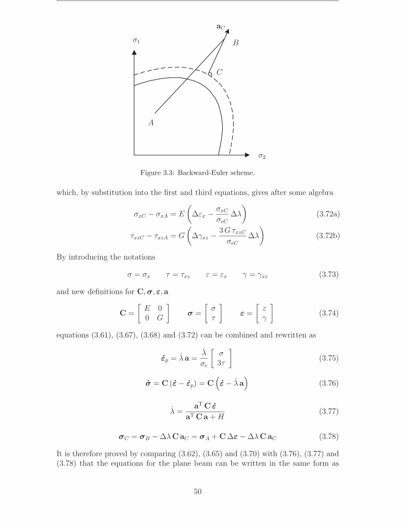
A

B

C

σ1

σ2

aC

Figure 3.3: Backward-Euler scheme.

which, by substitution into the first and third equations, gives after some algebra

σxC − σxA = E

(∆εx − σxC

σeC

∆λ

)(3.72a)

τxzC − τxzA = G

(∆γxz − 3 GτxzC

σeC

∆λ

)(3.72b)

By introducing the notations

σ = σx τ = τxz ε = εx γ = γxz (3.73)

and new definitions for C,σ, ε, a

C =

[E 00 G

]σ =

[στ

]ε =

[εγ

](3.74)

equations (3.61), (3.67), (3.68) and (3.72) can be combined and rewritten as

εp = λ a =λ

σe

[σ3τ

](3.75)

σ = C (ε − εp) = C(ε − λ a

)(3.76)

λ =aT C ε

aT Ca + H(3.77)

σC = σB − ∆λCaC = σA + C∆ε − ∆λCaC (3.78)

It is therefore proved by comparing (3.62), (3.65) and (3.70) with (3.76), (3.77) and(3.78) that the equations for the plane beam can be written in the same form as

50

those under plane stress conditions. It can be noted that the elastic forward step inthe backward-Euler scheme does not give σzB = 0, but the equation (3.78) provesthat σzB does not need to be calculated. A similar procedure is adopted in [23] toderive equations under plane stress condition from the three-dimensional case.

Backward-Euler scheme

The algorithm of the backward-Euler scheme is taken from [23], with the notationsintroduced at the end of the previous section.

The first estimation of σC is calculated with

σC = σB − ∆λCaB = σA + C∆ε − ∆λCaB (3.79)

where aB is calculated from (3.75) and ∆λ is determined from a first order Taylorexpansion of the yield function around point B

f = fB +∂fT

∂σ∆σB +

∂f

∂σo

∂σo

∂εps

∆εps = fB + aTB ∆σB − H ∆λ (3.80)

∆σB is then calculated from (3.76) as

∆σB = C (∆ε − ∆λ aB) (3.81)

with ∆ε = 0 since the total strain has already been applied in the elastic step (AB).Introducing (3.81) in (3.80) and setting f = 0 gives

∆λ =fB

aTB CaB + H

(3.82)

Equation (3.79) gives stresses which do not satisfy the yield function since the normalat B is not the same as the normal at the final position C.

The iterative process is performed by introducing the vector r defined by the differ-ence between the current stresses and the backward-Euler ones

r = σC − (σB − ∆λCaC) (3.83)

A truncated Taylor expansion of (3.83) gives

r = ro + σ + λCa + ∆λC∂a

∂σσ (3.84)

where

∂a

∂σ=

∂2f

∂σ2=

3

σ3e

[τ 2 −στ−στ σ2

](3.85)

and σ is the change in σC and λ is the change in ∆λ. The subscript C is fromnow dropped in order to simplify the notations (all the notations without subscriptsrefer to C). Setting r to zero in (3.84) gives

σ = −(I + ∆λC

∂a

∂σ

)−1 (ro + λCa

)= −Q−1

(ro + λCa

)(3.86)

51

A truncated Taylor expansion of the yield function at C gives

f = fo +∂fT

∂σσ +

∂f

∂σo

∂σo

∂εps

εps = fo + aT σ − H λ (3.87)

further, setting f = 0 and using (3.86) gives

λ =fo − aT Q−1 ro

aT Q−1 Ca + H(3.88)

The backward-Euler scheme is summarised by a flowchart in Figure 3.4.

Consistent tangent operator

The tangent operator Ct defined in equation (3.69) assumes infinitesimal strainand stress changes. However, in order to eliminate numerical elastic unloading, apath-independent strategy [28] is adopted. This means that at each iteration, thestrain changes are calculated with reference to the beginning of the increment (lastequilibrium state) and not with reference to the last iteration. This is the reasonwhy the use of Ct leads to low convergence rates for the Newton-Raphson method atthe structural level, unless the increments are infinitesimal. In order to maintain thequadratic convergence inherent in the Newton-Raphson method, a tangent operatorCct, consistent with the backward-Euler scheme is derived. The concept of consistenttangent operator has been first introduced by Simo and Taylor [90,91] and then usedby several authors. The derivation presented here follows [23].

Differentiation of (3.78) gives (subscript C is dropped)

σ = C ε − λCa − ∆λC∂a

∂σσ (3.89)

where the last term in equation (3.89) is omitted in the derivation of the standardtangent operator. From (3.89), it is obtained

σ =

(I + ∆λC

∂a

∂σ

)−1

C(ε − λ a

)= R

(ε − λ a

)(3.90)

The stresses must remain on the yield surface, which, from (3.64), gives

f = aT σ − H λ = aT + R(ε − λ a

)− H λ = 0 (3.91)

and hence

λ =aT R ε

aT Ra + H(3.92)

Introducing (3.92) in (3.90) finally gives

σ = Cct ε = R

(I − a aT R

aT Ra + H

)ε (3.93)

52

input

elastic predictor

σA εpsA ∆ε

σB = σA + C∆ε

σo = σY + H εpsA

(3.57) → fB

if fB > 0 first estimation

(3.75) → aB (3.82) → ∆λ

σ = σB − ∆λCaB

εps = εpsA + ∆λ

σo = σY + H εps

(3.57) → f

while f > 0 (tolerance)

(3.75) → a (3.83) → r

(3.85) → ∂a

∂σ(3.86) → Q

(3.88) → λ (3.86) → σ

∆λ = ∆λ + λ

εps = εpsA + ∆λ

σo = σY + H εps

(3.57) → f

Figure 3.4: Backward-Euler algorithm.

Chapter 4

3D beam element formulation

As for the 2D case, the main idea of the co-rotational approach in 3D [22,23,25,35,47,53,64,72,73,83,84,95] is to decompose the motion of the element into rigid body andpure deformational parts, through the use of a reference system which continuouslyrotates and translates with the element. The deformational response is captured atthe level of the local reference frame, whereas the geometric non-linearity induced bythe large rigid-body motion, is incorporated in the transformation matrices relatinglocal and global quantities. Assuming the pure deformation part to be small, alinear theory can be used from the onset in the local system. As pointed out byHaugen and Felippa in their review of the topic [43,44], the main benefit of such anassumption is the possibility to reuse existing high-performance linear elements.

In order to fully exploit this possibility, Rankin and co-workers [64,83,84] introducedthe so called “element independent co-rotational formulation”. The definition of theelement resorts to several changes of variables from the local frame to the global one.This is done through the use of a projector matrix which relates the variations ofthe local displacements to the variations of the global ones, by extracting the rigidbody modes from the latter. A very similar line of work was adopted by Pacosteand Eriksson [73] and will also be followed in this chapter. With respect to the citedreference, several improvements have been introduced.

The first one concerns the co-rotational framework. A different definition of the localcoordinate system is adopted. Besides, the number of local displacements is keptto seven (one translation and six rotations) and therefore, the projector matrix isnever explicitly computed. Instead, only certain block components in this matrix areevaluated and used directly in the expressions of the internal force vector and tangentstiffness in global coordinates. The objective here was to obtain a formulation whichis more efficient from a computational point of view. Rigid links and eccentric forcesare also introduced.

The second one is related to the parameterisation of finite 3D rotations. Thus, in [73]a 3-parameter representation based on the so-called “rotational vector”, is used.The main advantage here is that the rotational variables become additive and thenecessity of a special updating procedure is avoided. However, this parameterisationcan not be retained globally [51,73] as the magnitude of the rotational vector must be

55

restricted to values less than 2π. In order to overcome this inconvenience, a differentpossibility is explored in the present work. Essentially it amounts to using a vectorlike parameterisation but this time within each increment. Using the terminologyin [51], this alternative is based on the spatial form of the incremental rotationvector. Additive updates will still apply but this time only within an increment atthe level of the iterative corrections.

The third improvement is related to warping effects which are introduced by addinga seventh degree of freedom at each node of the element. With respect to [64, 73],this requires an adaptation of the co-rotational framework.

As already mentioned, the main feature of the adopted co-rotational formulation isits independence on the assumptions used to derive the internal forces and tangentstiffness in local coordinates. This means that for elements with the same numberof nodes and degrees of freedom the co-rotational framework is the same. Usingthis property, different local formulations can be tested and compared. In manyinstances, see e.g. [22,43,44,64,73], a linear strain definition is adopted in the localsystem. However, as the numerical applications will demonstrate, such a choicewill lead to incorrect results for certain classes of problems, especially when thetorsional effects are important. For this reason a different approach is advocated inthis work. At the level of the local frame, the kinematic description proposed byGruttmann et al. [41] is adopted and used to construct a consistent second orderapproximation to the Green-Lagrange strains. Various possibilities to simplify theresulting expressions are further discussed and tested in numerical examples.

The organisation of this chapter is as follows. Section 4.1 discusses some aspects re-lated to the parameterisation of finite 3D rotations, whereas the general co-rotationalframework for a two node beam element is introduced in Section 4.2. Section 4.3 isdevoted to the local element formulation in elasticity. Several local elements, basedon Timoshenko and Bernoulli assumptions and including or not warping effects arepresented. Based on the same strain assumptions as in elasticity, elasto-plastic localTimoshenko elements are derived in Section 4.4. Finally, Section 4.5 addresses cer-tain issues related to the applied external forces, e.g. rigid eccentricities, definitionof external moments.

4.1 Parameterisation of finite 3D rotations

One of the central issues in the development of a non-linear beam element is thetreatment of finite 3D rotations. In general, finite rotations are represented throughan orthogonal tensor R which is an element of the SO(3) rotation group. Its co-ordinate representation is a 3 × 3 orthogonal matrix involving nine components.However, owing to its orthonormality, it can be described in terms of only threeindependent parameters. One alternative in this context, is based on the so-called“rotational vector” [51,68,72,73], defined by

Ψ = uψ (4.1)

56

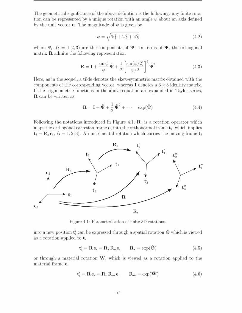
The geometrical significance of the above definition is the following: any finite rota-tion can be represented by a unique rotation with an angle ψ about an axis definedby the unit vector u. The magnitude of ψ is given by

ψ =√

Ψ21 + Ψ2

2 + Ψ23 (4.2)

where Ψi, (i = 1, 2, 3) are the components of Ψ. In terms of Ψ, the orthogonalmatrix R admits the following representation

R = I +sin ψ

ψΨ +

1

2

[sin(ψ/2)

ψ/2

]2

Ψ2

(4.3)

Here, as in the sequel, a tilde denotes the skew-symmetric matrix obtained with thecomponents of the corresponding vector, whereas I denotes a 3× 3 identity matrix.If the trigonometric functions in the above equation are expanded in Taylor series,R can be written as

R = I + Ψ +1

2Ψ

2+ · · · = exp(Ψ) (4.4)

Following the notations introduced in Figure 4.1, Ro is a rotation operator whichmaps the orthogonal cartesian frame ei into the orthonormal frame ti, which impliesti = Ro ei, (i = 1, 2, 3). An incremental rotation which carries the moving frame ti

e1

e3

e2

t3

t1

t2

t′3

t′1

t′2

t′′3

t′′1

t′′2

Ro

Rs

R

Rε

Figure 4.1: Parameterisation of finite 3D rotations.

into a new position t′i can be expressed through a spatial rotation Θ which is viewedas a rotation applied to ti

t′i = Rei = Rs Ro ei Rs = exp(Θ) (4.5)

or through a material rotation W, which is viewed as a rotation applied to thematerial frame ei

t′i = Rei = Ro Rm ei Rm = exp(W) (4.6)

57

In the terminology of Argyris [1], the sequence of rotation in equation (4.5) is denotedas “rotation around follower axes”, i.e. axes rotated by the previous rotation in thesequence, whereas the sequence described in equation (4.6) is denoted as “rotationaround fixed axes”, i.e. the rotation axes remain fixed but the rotation sequence itselfis inverted. The relationship connecting the spatial Θ and material W incrementalrotation vectors is thus given by

Θ = Ro W (4.7)

Let now consider an infinitesimal rotation which carries the frame t′i into t′′i , suchthat t′′i = Rε ei, (i = 1, 2, 3). Using the same dualism as above, admissible variationsδR are computed as

δR =d

dε[Rε]ε=0 =

d

dε

(exp(ε θ)R

)ε=0

= δθ R (4.8)

=d

dε(R exp(ε ω))ε=0 = R δω

where δω denotes material and δθ spatial angular variations, i.e. infinitesimal ro-tations superimposed onto the existing R. As defined in the above equation, theparameterisation of admissible variations δR is largely independent of the techniqueused to parameterise R itself. In order to obtain a consistent parameterisation, δθ(or alternatively δω) must be projected onto the parameter space adopted for R.This issue will be addressed in the remainder of this subsection, for the types ofparameterisation adopted in this work.

4.1.1 Rotational vector

Considering the spatial form of equation (4.8), admissible variations δΨ which leadto the same perturbed matrix Rε are found from

Rε = exp(Ψε) = exp(ε δθ)R (4.9)

where Ψε = Ψ + ε δΨ. Taking into account that R = exp(Ψ), this leads to

exp(ε δθ) = exp(Ψε) exp(−Ψ) (4.10)

Using the formula for compound rotations in terms of the rotational pseudo-vector(i.e. Rodrigues parameters) and differentiating with respect to ε, gives

δθ = Ts(Ψ) δΨ (4.11)

with

Ts(Ψ) =sin ψ

ψI +

(1 − sin ψ

ψ

)uuT +

1

2

(sin(ψ/2)

(ψ/2)

)2

Ψ (4.12)

Similar equations involving material angular variations δω can be easily derived bynoting that δθ = R δω. For details concerning the above derivation the interestedreader is referred to [51,72].

58

In connection with the linear operator Ts it should also be noted that

det(Ts) =2(1 − cos ψ)

ψ2(4.13)

which shows that the corresponding mapping ceases to be a bijection for ψ = 2kπ,k = 1, 2, ... [51, 72]. Avoiding these points, the inverse mapping is well defined as

δΨ = T−1s (Ψ) δθ (4.14)

with

T−1s =

(ψ/2)

tan(ψ/2)I +

(1 − (ψ/2)

tan(ψ/2)

)uuT − 1

2Ψ (4.15)

4.1.2 Incremental rotation vector

Considering equation (4.5), admissible variations δΘ which lead to the same per-turbed matrix Rε are found from

Rε = exp(Θε)Ro = exp(ε δθ)R (4.16)

where Θε = Θ + ε δΘ. Taking equation (4.5) into account leads to

exp(ε δθ) = exp(Θε) exp(−Θ) (4.17)

Following a procedure entirely similar to the one used in the preceding subsection(for details see [51]) leads to

δθ = Ts(Θ) δΘ (4.18)

Note that a similar relation connecting δω and δW can also be obtained. This issuehowever will not be further utilised in this thesis.

4.2 Co-rotational framework

The objective of this section is to define the co-rotational framework for a two nodebeam element. The central idea in this context is to introduce a local coordinatesystem which continuously rotates and translates with the element. With respect tothe moving frame, local (deformational) displacements pl are defined by extractingthe rigid body modes from the global displacements p g

g . The local displacementsare expressed as functions of the global ones, i.e.

pl = pl (pgg ) (4.19)

and used in order to compute the internal force vector fl and tangent stiffness matrixKl in local coordinates. Note that fl and Kl depend only on the definition of thelocal strains and not on the particular form of equation (4.19).

59

The expression of the internal force vector in global coordinates fg, can be obtainedby equating the internal virtual work in both the global and local systems

V = δpTl fl = δp g T

g fg (4.20)

Using equation (4.19), the connection between the variations of local and globaldisplacements is obtained as

δpl = B δp gg (4.21)

which, upon substitution into (4.20), provides the result of interest

fg = BT fl (4.22)

The expression of the tangent stiffness matrix in global coordinates Kg, is obtainedby taking the variations of equation (4.22), which gives

Kg = BT Kl B +∂B

∂p gg

: fl (4.23)

The second term on the right-hand side of the above equation is the so-called “geo-metric” stiffness, with the symbol “:” used to denote a contraction.

In equations (4.22) and (4.23), B and ∂B/∂p gg play the role of transformation ma-

trices required in order to re-express fl and Kl in global coordinates. These ma-trices, which actually define the co-rotational framework, depend on the non-linearfunctions in equation (4.19) and thus on the choice of the local coordinate system.However, they are independent of the particular strain definition used in order toderive fl and Kl. Consequently, various co-rotational elements defined using differ-ent local strain assumptions but the same type of local coordinate system will sharethe same transformation matrices, i.e. the co-rotational formulation is “element in-dependent” [64]. Using this property, various local assumptions can be placed atthe core of the co-rotational formulation and tested for efficiency and accuracy. Theissues pertaining to the development of a specific form for the local internal forcesfl and tangent stiffness Kl will however be addressed in the following sections.

The remainder of this section will instead focus on the definition of the co-rotationalframework. The approach put forth follows mainly [64, 73]. Thus, the change ofvariables (4.19) and subsequently the definition of the transformation matrices inequations (4.22) and (4.23) are performed by extracting the rigid body modes fromthe variations of the global displacements.

4.2.1 Coordinate systems, beam kinematics

The definition of the co-rotational two node beam element described in this section,involves several reference systems. First (see Figure 4.2), a global reference systemdefined by the triad of unit orthogonal vectors eα, α = 1, 2, 3. Second, a local systemwhich continuously rotates and translates with the element. The orthonormal basis

60

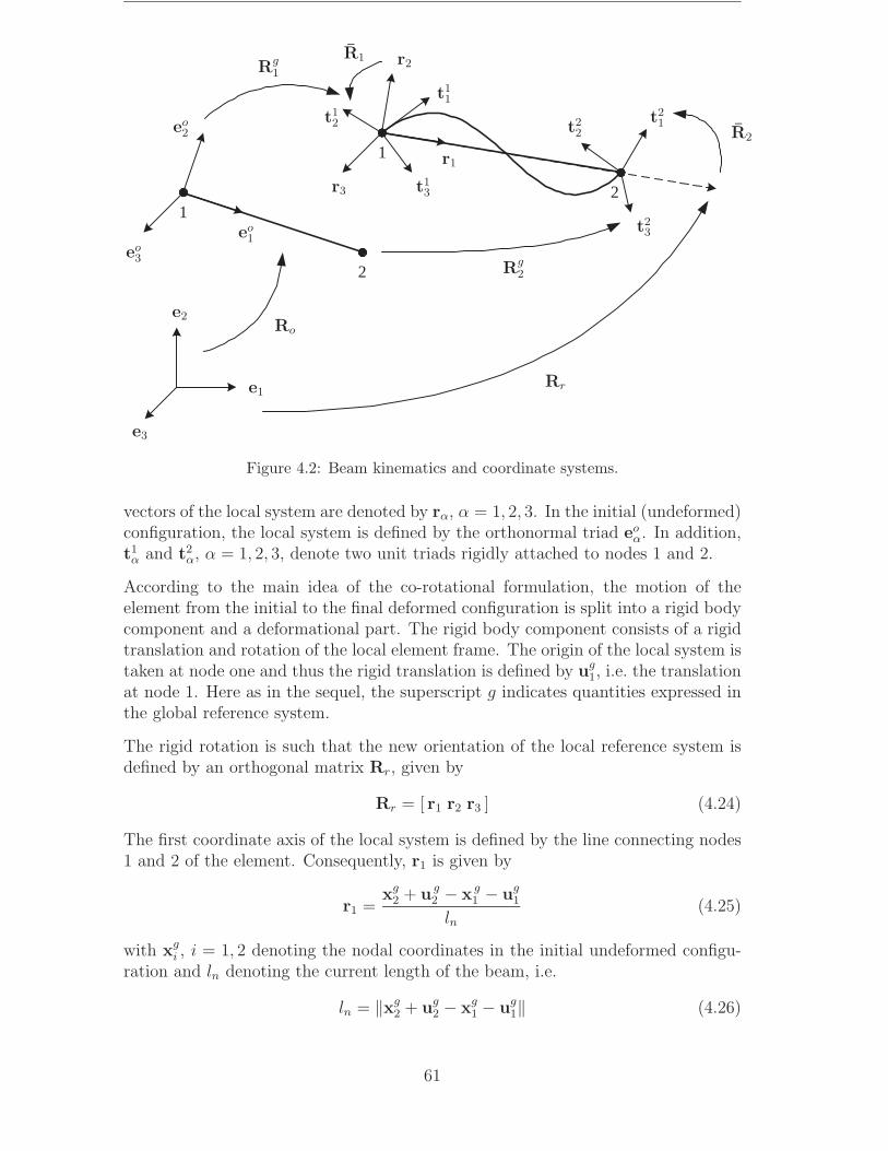
1

1

2

2

e3

e1

e2

eo1

eo2

eo3

r1

r3

r2

t23

t21t2

2

t13

t11

t12

Ro

Rr

Rg2

Rg1

R2

R1

Figure 4.2: Beam kinematics and coordinate systems.

vectors of the local system are denoted by rα, α = 1, 2, 3. In the initial (undeformed)configuration, the local system is defined by the orthonormal triad eo

α. In addition,t1α and t2

α, α = 1, 2, 3, denote two unit triads rigidly attached to nodes 1 and 2.

According to the main idea of the co-rotational formulation, the motion of theelement from the initial to the final deformed configuration is split into a rigid bodycomponent and a deformational part. The rigid body component consists of a rigidtranslation and rotation of the local element frame. The origin of the local system istaken at node one and thus the rigid translation is defined by ug

1, i.e. the translationat node 1. Here as in the sequel, the superscript g indicates quantities expressed inthe global reference system.

The rigid rotation is such that the new orientation of the local reference system isdefined by an orthogonal matrix Rr, given by

Rr = [ r1 r2 r3 ] (4.24)

The first coordinate axis of the local system is defined by the line connecting nodes1 and 2 of the element. Consequently, r1 is given by

r1 =xg

2 + u g2 − x g

1 − ug1

ln(4.25)

with xgi , i = 1, 2 denoting the nodal coordinates in the initial undeformed configu-

ration and ln denoting the current length of the beam, i.e.

ln = ‖xg2 + ug

2 − xg1 − ug

1‖ (4.26)

61

The remaining two axes are determined with the help of an auxiliary vector q. Inthe initial configuration q is directed along the local eo

2 direction, whereas in thedeformed configuration its orientation is obtained from

q =1

2(q1 + q2) qi = Rg

i Ro [ 0 1 0 ]T i = 1, 2 (4.27)

where Rg1 and Rg

2 are the orthogonal matrices used to specify the orientation of thenodal triads t1

α and t2α respectively, and Ro specifies the orientation of the local

frame in the initial configuration, i.e. Ro = [ eo1 eo

2 eo3 ]. The unit vectors r2 and r3

are then computed by the vector products

r3 =r1 × q

‖r1 × q‖ r2 = r3 × r1 (4.28)

and the orthogonal matrix Rr in equation (4.24) is completely determined.

The rigid motion previously described, is accompanied by local deformational dis-placements with respect to the local element axes. In this context, due to theparticular choice of the local system, the local translations at node 1 will be zero.Moreover, at node 2, the only non zero component is the translation along r1. Thiscan easily be evaluated according to

u = ln − lo (4.29)

with lo denoting the length of the beam in the original undeformed configuration.Here as in the sequel, an overbar denotes a deformational kinematic quantity.

The global rotations at node i can be expressed in terms of the rotation of the localaxes, defined by Rr, followed by a local rotation relative to these axes; this is definedby the orthogonal matrix Ri. Using the terminology of Section 4.1, the latter shouldbe viewed as a material rotation. Consequently, the orientation of the nodal triadtiα can be obtained by means of the product Rr Ri. On the other hand, (see Figure

4.2) this orientation can also be obtained through the product Rgi Ro, which gives

Ri = RTr Rg

i Ro i = 1, 2 (4.30)

The local rotations are then evaluated from

ϑi = log(Ri

)i = 1, 2 (4.31)

The explicit form of equation (4.19) is thus completely specified through equations(4.29), (4.30) and (4.31), with pl given by

pl =[u ϑ

T1 ϑ

T2

]T(4.32)

Correspondingly, the local internal force vector is given by

fl =[n mT

1 mT2

]T(4.33)

where n denotes the axial force whereas m1 and m2 denote the moments at nodes1 and 2, respectively.

62

The next step will then be to determine the transformation matrix B in equation(4.21). This matrix relates the variations of the local displacements

δpl =[δu δϑ

T1 δϑ

T2

]T(4.34)

to their global counterparts

δp gg =

[δug T

1 δθ g T1 δug T

2 δθ g T2

]T(4.35)

with δθ gi , i = 1, 2 denoting spatial angular variations as defined in (4.8). The

expression of B, and subsequently the transformations in equations (4.22) and (4.23)are derived using a sequence of two changes of variables, as described in the followingsubsections.

4.2.2 Change of variables δϑ −→ δθ

The general procedure for evaluating the transformation matrix B involves the vari-ations of equations (4.29) and (4.30). Referring to (4.30), admissible variations δRi,i = 1, 2 are computed – cf. equation (4.8) – according to

δRi = δ ˜θi Ri (4.36)

The angular variations δθi involved in the above equation, are of a different naturethan δϑi as defined in (4.31). A change of variables from δϑi to δθi is thus required.In order to construct such a change of variables, using equations (4.14), (4.31) and(4.36), δθi and δϑi are connected by

δϑ = T−1s (ϑ) δθ (4.37)

which, by introducing the notation

δpa =[δu δθ

T1 δθ

T2

]T(4.38)

gives

δpl = Ba δpa Ba =

1 01,3 01,3

03,1 T−1s (ϑ1) 0

03,1 0 T−1s (ϑ2)

(4.39)

Here, as in the sequel 0i,j denotes an i× j zero matrix. For a 3× 3 zero matrix thenotation 0 is however used.

Further, a virtual work equation gives

fa = BTa fl (4.40)

63

with fa denoting the internal force vector consistent with δpa. The correspondingtransformation for the local tangent stiffness matrices, i.e. Kl and Ka, is obtainedby taking the variations of (4.40)

δfa = BTa δfl + δBT

a fl (4.41)

where, by definition

δfl = Kl δpl δfa = Ka δpa (4.42)

Using equations (4.39), (4.41) and (4.42) gives the required transformation

Ka = BTa Kl Ba + Kh Kh =

0 01,3 01,3

03,1 Kh1 0

03,1 0 Kh2

(4.43)

The expressions of Kh1 and Kh2 are computed from

∂

∂θ[T−T

s v] =∂

∂ϑ[T−T

s v]∂ϑ

∂θ=

∂

∂ϑ[T−T

s v]T−1s (4.44)

with the vector v maintained constant during differentiation. Using (4.14) givesafter some algebra

∂

∂θ[T−T

s v] =

[η [ϑvT − 2v ϑ

T+ (ϑ

T · v) I] + µ ˜ϑ2[v ϑ

T] − 1

2v

]T−1

s (ϑ) (4.45)

with the coefficients η and µ given by

η =2 sin α − α (1 + cos α)

2 α2 sin αµ =

α (α + sin α) − 8 sin2(α/2)

4 α4 sin2(α/2)α = ‖ϑ‖ (4.46)

Thus, Khi, i = 1, 2 are evaluated from equation (4.45) with ϑ = ϑi and v = mi,with mi as defined in (4.33).

Finally, it should be mentioned that, at least for small increments, ϑ is a smallquantity. Consequently, T−1

s (ϑ) is close to identity. For this reason, the transfor-mation described by equations (4.40) and (4.43) is often omitted in the formulationof co-rotational elements (cf. e.g. [22]). The numerical tests performed in [73] showedthat this omission has scarcely any effect on the correctness of the results, althoughit has an impact on the convergence properties of the element.

4.2.3 Change of variables δpa −→ δp gg

The second step of the variable change involves δpa and δp gg , as defined in equations

(4.38) and (4.35), respectively.

Referring first to the local axial translation u, the variations of equation (4.29) give

δu = δln = r δp gg r =

[−rT1 01,3 rT

1 01,3

](4.47)

64

For the rotational terms, the variations of equation (4.30) are needed

δRi = δRTr Rg

i Ro + RTr δRg

i Ro (4.48)

where δRi is defined in (4.36) whereas δRgi and δRr are computed using the spatial

form of equation (4.8), i.e.

δRgi = δθ

g

i Rgi δRr = δθ

g

r Rr (4.49)

δRTr is calculated from the orthogonality condition Rr RT

r = I which, by differenti-ation and introduction of (4.49) gives

δRr RTr + Rr δRT

r = 0 (4.50a)

δθg

r Rr RTr + Rr δRT

r = 0 (4.50b)

and then

δRTr = −RT

r δθg

r (4.51)

Using (4.36), (4.49) and (4.51), equation (4.48) can be rewritten as

δ ˜θi Ri = −RTr δθ

g

r Rgi Ro + RT

r δθg

i Rgi Ro

= −RTr δθ

g

r Rr RTr Rg

i Ro + RTr δθ

g

i Rr RTr Rg

i Ro (4.52)

= (δθe

i − δθe

r ) Ri

where use has been made of equation (4.30) and of the fact that Rr transforms avector and a tensor from global to local coordinates according to

xe = RTr xg xe = RT

r xg Rr (4.53)

Thus, equation (4.52) gives

δθi = δθ ei − δθ e

r i = 1, 2 (4.54)

Further, let

δp eg = ET δp g

g E =

Rr 0 0 0

0 Rr 0 0

0 0 Rr 0

0 0 0 Rr

(4.55)

Then, using the chain rule, δθi is evaluated as

δθi =∂θi

∂p eg

∂p eg

∂p gg

δp gg =

∂θi

∂p eg

ET δp gg i = 1, 2 (4.56)

Substituting from equation (4.54) gives[δθ1

δθ2

]=

([0 I 0 0

0 0 0 I

]−[

GT

GT

])ET δp g

g = PET δp gg (4.57)

65

where the matrix G is defined by

G =∂θ e

r

∂p eg

(4.58)

Hence, from (4.47) and (4.57), the connection between δpa and δp gg is given by

δpa = Bg δp gg Bg =

[r

PET

](4.59)

Expression of G

The expression of G is obtained from (4.49) which can be rewritten as

δθg

r = δRr RTr (4.60)

and after the transformation (4.53) as

δθe

r = RTr δRr (4.61)

From (4.24) and the above equation, it can easily be found that

δθ er =

δθ er1

δθ er2

δθ er3

=

−rT2 δr3

−rT3 δr1

rT2 δr1

(4.62)

Introducing the notation ugi = [ ug

i1 ugi2 ug

i3 ]T (i = 1, 2), differentiation of (4.25) gives

δrg1 =

1

ln

[I − r1 rT

1

]

δug21 − δug

11

δug22 − δug

12

δug23 − δug

13

(4.63)

and after transformation (4.53) in the local coordinate system, it is obtained

δre1 =

1

ln

δue21 − δue

11

δue22 − δue

12

δue23 − δue

13

(4.64)

Hence, since the local expressions of r2 and r3 are [ 0 1 0 ]T and [ 0 0 1 ]T, equation(4.62) gives

δθ er2

=1

ln(δue

13 − δue23) (4.65a)

δθ er3

=1

ln(δue

22 − δue12) (4.65b)

66

The evaluation of δθ er1

is more complicated and can be performed as follows. Differ-entiation of (4.27) gives

δq =1

2(δRg

1 + δRg2)Ro [ 0 1 0 ]T

=1

2(δθ

g

1 Rg1 + δθ

g

2 Rg2)Ro [ 0 1 0 ]T (4.66)

=1

2(δθ

g

1 q1 + δθg

2 q2)

The local expressions of the vectors q, q1 and q2 are denoted by

RTr q =

q1

q2

0

RT

r q1 =

q11

q12

q13

RT

r q2 =

q21

q22

q23

(4.67)

The last coordinate of RTr q is zero since q is perpendicular to r3.

The local expression of δq can be deduced from equation (4.66) as

δqe =1

2δθ

e

1

q11

q12

q13

+

1

2δθ

e

2

q21

q22

q23

(4.68)

which after calculation gives

δqe =1

2

− q12 δθ e13 + q13 δθ e

12 − q22 δθ e23 + q23 δθ e

22

+ q11 δθ e13 − q13 δθ e

11 + q21 δθ e23 − q23 δθ e

21

− q11 δθ e12 + q12 δθ e

11 − q21 δθ e22 + q22 δθ e

21

(4.69)

The following notations are introduced

η =q1

q2

η11 =q11

q2

η12 =q12

q2

η21 =q21

q2

η22 =q22

q2

(4.70)

The differentiation of r3 is calculated from its definition (4.28). By noting that‖r1 × q‖ = q2, the first line of equation (4.62) can be rewritten as

δθ er1

= −rT2

q2

δre1 × q − rT

2

q2

r1 × δqe − δ

(1

q2

)rT2 (r1 × q) (4.71)

The last term in the above equation is zero. The two others terms can be evaluatedfrom equations (4.64), (4.67) and (4.69). The result, after some work, is

δθ er1

=η

ln(δwe

1 − δwe2) −

η11

2δθ e

12 +η12

2δθ e

11 −η21

2δθ e

22 +η22

2δθ e

21 (4.72)

Finally, the expression for the matrix G is

GT =

0 0η

ln

η12

2−η11

20 0 0 − η

ln

η22

2−η21

20

0 01

ln0 0 0 0 0 − 1

ln0 0 0

0 − 1

ln0 0 0 0 0

1

ln0 0 0 0

(4.73)

67

Internal forces

Using (4.59), the internal force vector in global coordinates is computed as

fg = BTg fa (4.74)

Note that, according to the sequence of variable changes previously defined, thematrix B in equation (4.21) is explicitly given by the product Ba Bg.

Tangent stiffness matrix

Differentiation of (4.74) gives

δfg = BTg Ka Bg δp g

g + δrT fa1 + δ(EPT)m (4.75)

with

m =[

fa2 fa3 fa4 fa5 fa6 fa7

]T(4.76)

where fai, i = 1, 7 denotes the i-th component of the vector fa.

From (4.47) and (4.63), it can easily be derived that

δrT = D δp gg D =

D3 0 −D3 0

0 0 0 0

−D3 0 D3 0

0 0 0 0

D3 =

1

ln(I − r1 rT

1 ) (4.77)

The last term in expression (4.75) is evaluated from

δ(EPT)m = δEPT m + E δPT m (4.78)

By introducing

PT m =

n1

m1

n2

m2

(4.79)

and using (4.55) and (4.61), the first term in (4.78) can be expressed as

δEPT m =

Rr δθe

r 0 0 0

0 Rr δθe

r 0 0

0 0 Rr δθe

r 0

0 0 0 Rr δθe

r

n1

m1

n2

m2

= E

δθe

r n1

δθe

r m1

δθe

r n2

δθe

r m2

(4.80)

which, using the relation

a b = −b a (4.81)

68

gives

δEPT m = −EQ δθ er Q =

n1

m1

n2

m2

(4.82)

Then, by using (4.58), it is obtained

δEPT m = −EQGT ET δp gg (4.83)

The calculation of the second term of (4.78) requires the value of δPT which can beobtained by introducing the matrix A such as

AT =

0 0 0 0 0 0 0 0 0 0 0 0

0 0 0 0 0 0 0 0 −ln 0 0 0

0 0 0 0 0 0 0 ln 0 0 0 0

(4.84)

and by noting that

AT G = I (4.85)

Differentiation of the above equation gives

δAT G + AT δG = 0 (4.86)

and hence

δG = −A−T δAT G = −G δAT G (4.87)

Further, using the definition of P in (4.57) gives

δP = −C δGT C =

[I

I

](4.88)

which can be rewritten as

δPT = −δGCT = G δAT GCT (4.89)

Then, the second term of (4.78) becomes

E δPT m = EG δAT GCT m (4.90)

which can be simplified after symbolic matrix multiplications as

E δPT m = EGa δln (4.91)

with

a =

0

η

ln(fa2 + fa5) −

1

ln(fa3 + fa6)

1

ln(fa4 + fa7)

(4.92)

69

Introducing (4.47) in (4.91) gives

E δPT m = EGar δp gg (4.93)

Finally, from equations (4.75), (4.78), (4.83) and (4.93) the expression of the globaltangent stiffness matrix is

Kg = BTg Ka Bg + Km Km = D fa1 − EQGT ET + EGar (4.94)

Note that the tangent stiffness matrix as given by equation (4.94), is not symmet-ric. However, as shown in [64], it can be symmetrised without losing quadraticconvergence unless concentrated moments are applied on the structure.

4.2.4 Eccentric nodes, rigid links

A beam element is defined such that node 1 is rigidly linked to another node I ofthe structure. Mathematically this can be expressed as

xgI = xg

1 + vo (4.95)

where xg1 and xg

I denote the position vectors of nodes 1 and I in the original un-deformed configuration whereas vo denotes an eccentricity vector. Since the link isassumed as rigid, the magnitude of the eccentricity vector will not change duringthe deformation of the structure. The connection between the displacements at thetwo nodes 1 and I can then be expressed as

ugI = ug

1 + (Rg1 − I) vo Rg

1 = RgI (4.96)

The modelling of a rigid link will thus require a change of variables from ug1 to ug

I .Taking the variations of equation (4.96), and using (4.81), gives

δugI = δug

1 + δRg1 vo = δug

1 + δθg

1 Rg1 vo = δug

1 − v δθ g1 (4.97)

with

v = Rg1 vo (4.98)

which, by introducing the notation

δp gec =

[δug T

I δθ g T1 δug T

2 δθ g T2

]T(4.99)

leads to

δp gg = Bec δp g

ec Bec =

I v 0 0

0 I 0 0

0 0 I 0

0 0 0 I

(4.100)

70

with δp gg as defined in equation (4.35). The internal force vector fec and tangent

stiffness matrix Kec consistent with δp gec are then given by

fec = BTec fg Kec = BT

ec Kg Bec + Kn (4.101)

The matrix Kn is calculated by

Kn δp gec = δ(BT

ec) fg =

03,1

−δv n

03,1

03,1

=

03,1

n δθg

1 v

03,1

03,1

=

03,1

−n v δθ g1

03,1

03,1

=

0 0 0 0

0 −n v 0 0

0 0 0 0

0 0 0 0

δp g

ec

(4.102)

with n = [ fg1 fg2 fg3 ]T, fgii = 1, 12 denotes the i-th component of the vector fg.

4.2.5 Finite rotation parameters

The global internal force vector fg and tangent stiffness matrix Kg computed ac-cording to equations (4.74) and (4.94) are consistent with spatial angular variationsδθ g of the type defined in the first of equations (4.8). Consequently, for a certainnode of the structure, the updating of the rotation matrix at each iteration stepwould have to be done according to

Rgn = exp(δθ

g)Rg

o (4.103)

where the subscripts n and o denote quantities corresponding to the “new” and“old” configurations, respectively. Note that in this case the parameterisation of Rg

is largely independent on the technique used to parameterise its admissible varia-tions. Using the terminology in [51], this alternative will be denoted as “intrinsic”parameterisation of 3D rotations.

In addition to the “intrinsic” parameterisation, two alternatives are explored in thepresent work. The first one is based on the rotation vector Ψ g, i.e. a 3-parameterrepresentation, cf. (4.3). In this case, the rotational variables are additive and thenecessity of a special updating procedure is avoided. The second alternative is basedon the spatial form of the incremental rotation vector Θ g, cf. (4.5) [51,68]. The rota-tional variables are still additive, but this time only within an increment at the levelof the iterative corrections. Corresponding to these two choices, additional changesof variables from δθ g to δΨ g or alternatively from δθ g to δΘ g, must be introduced.These changes of variables are defined in the remainder of this subsection.

It should be noted here that in the context of multi-parametric analyses of instabilityproblems, additive variables, at least at the level of iterative corrections, are essential

71

for an efficient implementation of fold line evaluation algorithms [68, 71]. In thecontext of dynamical problems and Newmark time-stepping schemes, an excellentdiscussion on the relative merits of the different alternatives is presented in [51].

Change of variables: δθ g −→ δΨ g

For the purposes of this subsection, let p gr denote the following vector of global

nodal displacements

p gr =

[ug T

1 Ψ g T1 ug T

2 Ψ g T2

]T(4.104)

where Ψ gi denotes the rotational vector at node i. The change to the new kinematic

variables in p gr requires the connection between δp g

g as defined in (4.35) and δp gr .

This connection can be easily constructed using (4.11)

δp gg = Br δp g

r Br =

I 0 0 0

0 Ts(Ψg1 ) 0 0

0 0 I 0

0 0 0 Ts(Ψg2 )

(4.105)

The global internal force vector fr and tangent stiffness matrix Kr, consistent withp g

r , are then given by

fr = BTr fg Kr = BT

r Kg Br + Kv (4.106)

where

Kv =

0 0 0 0

0 Kv1 0 0

0 0 0 0

0 0 0 Kv2

(4.107)

The expressions of Kv1 and Kv2 are obtained from

∂

∂Ψ[TT

s v] = −(

sin ψ

ψ−(

sin(ψ/2)

(ψ/2)

)2)

(u × v)uT +1

2

(sin(ψ/2)

(ψ/2)

)2

v

+

(cos ψ − sin ψ

ψ

)1

ψ

[vuT − (uTv)uuT

](4.108)

+

(1 − sin ψ

ψ

)1

ψ

[uvT − 2 (uTv)uuT + (uTv) I

]with the vector v maintained constant during the differentiation.

Thus, Kv1 and Kv2 are evaluated from equation (4.108) with Ψ = Ψ g1 and Ψ = Ψ g

2 ,respectively and v = [ fg4 fg5 fg6 ]T , v = [ fg10 fg11 fg12 ]T , respectively.

72

With this new parameterisation, the rotational variables are additive and the itera-tive updates are performed according to

Ψ gn = Ψ g

o + δΨ g Rgn = exp(Ψ g

n) (4.109)

The main drawback of a parameterisation based on the rotation vector lies in thefact that it cannot be retained globally. As implied by equation (4.13), the linearoperator Ts becomes singular if the magnitude of the rotation vector reaches 2π.This undesirable feature is then passed over to the tangent stiffness matrix computedaccording to equation (4.106). In order to remove this drawback, a parameterisa-tion based on the incremental rotation vector Θ g and its iterative increment δΘ g,cf. subsection 4.1.2, will be discussed in the next subsection.

Change of variables: δθ g −→ δΘ g

The transformation matrices required in this second case are constructed on the basisof equation (4.18) which provides the connection between δθ g and δΘ g. Followinga procedure entirely similar to that used in the preceding subsection, the vector p g

r

is now defined as

p gr =

[ug T

1 Θ g T1 ug T

2 Θ g T2

]T(4.110)

where Θ gi denotes the spatial form of the incremental rotation vector at node i.

Note that in order to avoid singularities in the expression of T s, the magnitudeof Θ g should be restricted to values less than 2π. Since Θ g now represents anincremental rotation between two consecutive equilibrium states, this restriction isof no practical consequence.

The transformation equations for the internal force vector and the tangent stiffnessmatrix are formally identical to equations (4.105)–(4.108), by replacing Ψ g

i by Θ gi .

Using the incremental rotation vector, additive updates apply only within an in-crement at the level of the iterative corrections. Thus, the updating of the nodalrotations is performed according to

Θ gn = Θ g

o + δΘ g Rgn = exp(Θ g

n)Rgn−1 (4.111)

where Rgn−1 is the rotational matrix obtained at the end of the previous increment.

The transformation matrices required for this second type of parameterisation areessentially constructed using the same linear operators as before, which considerablysimplifies the implementation.

4.2.6 Formulation with warping

In order to include warping effects, additional (warping) degrees of freedom αi areintroduced at both nodes i = 1, 2 of the element. The local displacement vector will

73

thus become

p ∗l =

[u ϑ

T1 ϑ

T2 α1 α2

]T(4.112)

However, since the warping is in itself a deformational quantity, these additional de-grees of freedom remain constant during the sequence of transformations previouslydefined. Hence, referring for instance to equation (4.59), the variations δpa and δp g

g

are rewritten as

δp ∗a =

[δu δθ

T1 δθ

T2 δα1 δα2

]T(4.113a)

δp g ∗g =

[δug T

1 δθ g T1 δug T

2 δθ g T2 δα1 δα2

]T(4.113b)

and the corresponding connection is defined by

δp ∗a = B ∗

g δp g ∗g B ∗

g =

[Bg 02

02 I2

](4.114)

with Bg as given in (4.59) and I2 denoting a 2×2 identity matrix. Including warpingeffects, the global internal force vector and tangent stiffness matrix are given by

f ∗g = B ∗T

g f ∗a K ∗

g = B ∗Tg K ∗

a B ∗g + K ∗

m K ∗m =

[Km 02

02 02

](4.115)

with Km as defined in equation (4.94). The two other transformations are modifiedin a similar way.

4.3 Local element formulation in elasticity

The purpose of this section is to define the internal force vector fl (f ∗l if warping

effects are considered) and tangent stiffness matrix Kl (K ∗l ) in local coordinates.

Assuming elastic material behaviour, fl and Kl can be derived from the strain energyΦ expressed as a function of the local displacements pl (or alternatively p ∗

l ), throughsuccessive differentiations

fl =∂Φ

∂pl

Kl =∂2Φ

∂p2l

(4.116)

For all element types presented in this section, the differentiations involved in equa-tion (4.116) have been performed using the Maple symbolic software package. Forthis reason, explicit expressions for fl and Kl will not be provided here. The remain-der of this section will instead focus on the strain energy expression which is thekeystone in constructing the necessary Maple subroutines. To complete the elementdefinition, the Maple codes are given in Appendix A.

In order to provide an explicit expression for Φ(pl), a certain definition of the localstrains must be adopted. As the main interest of the co-rotational formulation lies

74

in the fact that the geometrical non-linearity is embedded in the motion of the localelement frame, the local strains can be expressed in a simple manner. In fact, mostof the co-rotational elements found in the literature are based on local linear strainassumptions. However, as the numerical tests presented in this thesis will show,such elements can give inaccurate results for problems where the torsion effects areimportant. For these reasons, in the present work a second order approximation ofthe Green-Lagrange strains is constructed at the level of the local element frame.The resulting expressions are subsequently simplified by neglecting certain secondorder terms. The effects of these simplifications are then carefully examined in thenumerical examples.

4.3.1 Local beam kinematics, strain energy

As a general rule, all kinematic quantities introduced in this subsection are referredto the local element frame ri, i = 1, 2, 3, as defined in equations (4.25), (4.27)and (4.28). The origin of the local system is taken at node 1 with r1 directed alongthe line of centroids. Note however that r2 and r3 are not necessarily directed alongthe principal axes of the cross-section.

With respect to the local system, the Green-Lagrange strain components whichcontribute to the strain energy of the beam are given by

ε11 = u1,1 +1

2u2

1,1 +1

2u2

2,1 +1

2u2

3,1

2 ε12 = u1,2 + u2,1 + u1,1 u1,2 + u2,1 u2,2 + u3,1 u3,2 (4.117)

2 ε13 = u1,3 + u3,1 + u1,1 u1,3 + u2,1 u2,3 + u3,1 u3,3

where u1, u2, u3 are the local (deformational) displacements of the current point P .In the above equation, a comma followed by an index denotes differentiation withrespect to the corresponding variable.

In order to obtain a consistent second order approximation of the strain expressionsin equation (4.117), a second order approximation of the displacement field is needed.Within the settings of classical beam theory, cf. e.g. [4], bending is defined around thecentroid G while torsion is referred to the shear center C. Consequently, wheneverC and G are not coincident, the derivation of a non-linear displacement field is notan easy task since rotations are not defined around the same point. An attemptcan be found in [60], but the approach presented there lacks consistency. In fact,with the classical beam theory, only a linearised displacement field, obtained bysuperposition of linear stretching, bending and torsional effects can be derived.

In order to avoid such problems, the kinematic model proposed by Gruttmann etal. [41] is adopted, see Figure 4.3. Thus, let xo

P (x1, x2, x3) denote the position vectorof point P in the initial (i.e. rotated but still undeformed) configuration and letxP (x1, x2, x3) denote the position vector of P in the current configuration. These

75

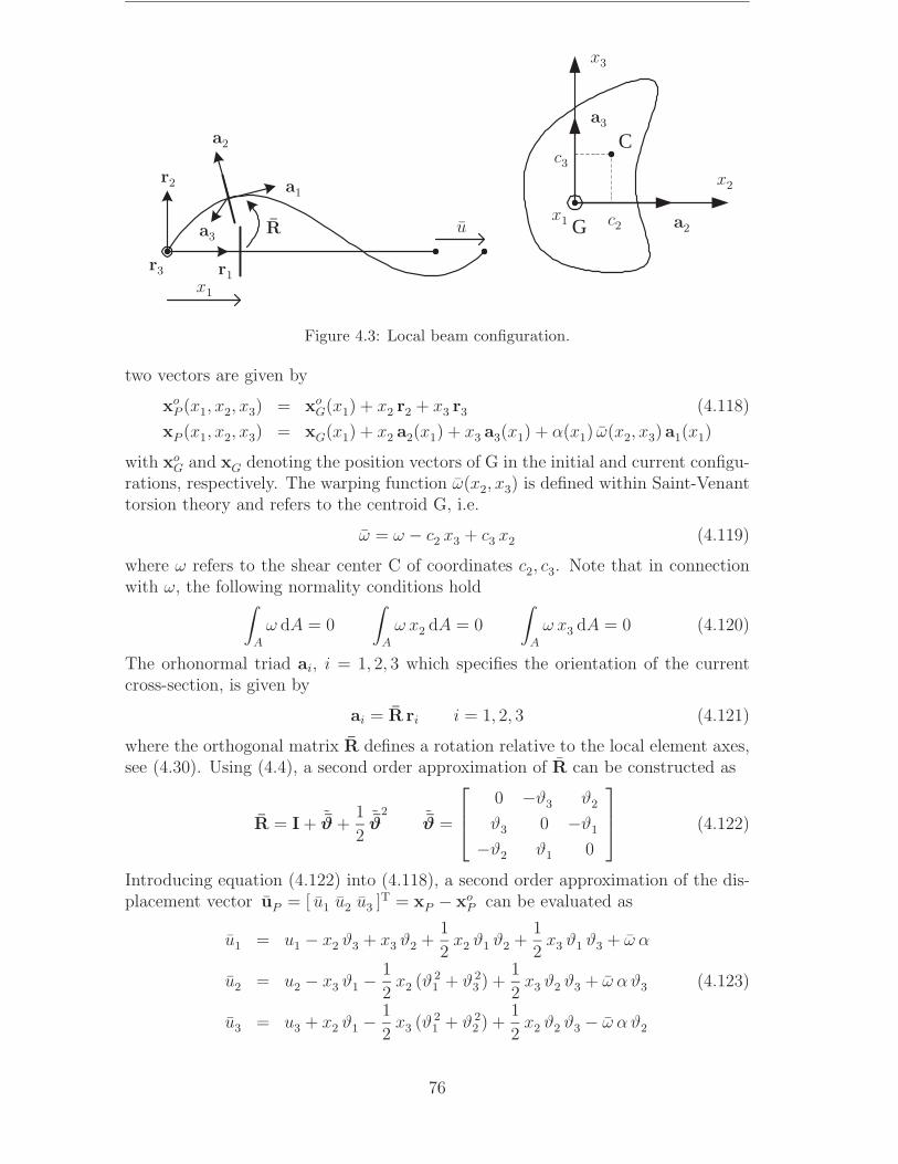
G

C

r1

r2

r3

a1

a2

a2a3

a3

R

x1

x1

x2

x3

c2

c3

u

Figure 4.3: Local beam configuration.

two vectors are given by

xoP (x1, x2, x3) = xo

G(x1) + x2 r2 + x3 r3 (4.118)

xP (x1, x2, x3) = xG(x1) + x2 a2(x1) + x3 a3(x1) + α(x1) ω(x2, x3) a1(x1)

with xoG and xG denoting the position vectors of G in the initial and current configu-

rations, respectively. The warping function ω(x2, x3) is defined within Saint-Venanttorsion theory and refers to the centroid G, i.e.

ω = ω − c2 x3 + c3 x2 (4.119)

where ω refers to the shear center C of coordinates c2, c3. Note that in connectionwith ω, the following normality conditions hold∫

A

ω dA = 0

∫A

ω x2 dA = 0

∫A

ω x3 dA = 0 (4.120)

The orhonormal triad ai, i = 1, 2, 3 which specifies the orientation of the currentcross-section, is given by

ai = R ri i = 1, 2, 3 (4.121)

where the orthogonal matrix R defines a rotation relative to the local element axes,see (4.30). Using (4.4), a second order approximation of R can be constructed as

R = I + ˜ϑ +1

2˜ϑ

2 ˜ϑ =

0 −ϑ3 ϑ2

ϑ3 0 −ϑ1

−ϑ2 ϑ1 0

(4.122)

Introducing equation (4.122) into (4.118), a second order approximation of the dis-placement vector uP = [ u1 u2 u3 ]T = xP − xo

P can be evaluated as

u1 = u1 − x2 ϑ3 + x3 ϑ2 +1

2x2 ϑ1 ϑ2 +

1

2x3 ϑ1 ϑ3 + ω α

u2 = u2 − x3 ϑ1 −1

2x2 (ϑ 2

1 + ϑ 23 ) +

1

2x3 ϑ2 ϑ3 + ω α ϑ3 (4.123)

u3 = u3 + x2 ϑ1 −1

2x3 (ϑ 2

1 + ϑ 22 ) +

1

2x2 ϑ2 ϑ3 − ω α ϑ2

76

where u1, u2, u3 are the displacements of the centroid G, i.e. the components of thevector xG − xo

G.

Using equations (4.119), (4.120) and (4.123), a second order approximation of theGreen-Lagrange strains defined in (4.117) can be evaluated. At this level, two ad-ditional simplifications are introduced. First, the term 1/2 u2

1,1 in the expression ofε11 is neglected. Second, the non-linear strain components generated by warping areomitted since warping effects are rationally taken into account in a linearised wayonly [42]. Using these simplifications gives

ε11 = εc + x2 k2 + x3 k3 +1

2r2 ϑ 2

1,1 + ω α,1

2 ε12 = γ12 + ω,2 α − x3 k1 (4.124)

2 ε13 = γ13 + ω,3 α + x2 k1

with

r2 = x22 + x2

3

εc = u1,1 +1

2

(u2

2,1 + u23,1

)k2 = −ϑ3,1 +

1

2

(ϑ1,1 ϑ2 + ϑ1 ϑ2,1

)+ u3,1 ϑ1,1 + c3 α,1

k3 = ϑ2,1 +1

2

(ϑ1,1 ϑ3 + ϑ1 ϑ3,1

)− u2,1 ϑ1,1 − c2 α,1 (4.125)

k1 = ϑ1,1 +1

2

(ϑ2,1 ϑ3 − ϑ2 ϑ3,1

)γ12 = u2,1 − ϑ3 +

1

2ϑ1 ϑ2 + u3,1 ϑ1 − u1,1 ϑ3

γ13 = u3,1 + ϑ2 +1

2ϑ1 ϑ3 − u2,1 ϑ1 + u1,1 ϑ2

The strain energy can then be evaluated from

Φ =

∫lo

ΦA dx1 =

∫lo

(1

2E

∫A

ε 211 dA +

1

2G

∫A

[(2ε12)

2 + (2ε13)2] dA

)dx1 (4.126)

Integration through the cross-section gives∫A

ε 211 dA = Aε2

c + I22 k22 + I33 k2

3 +1

4Irr ϑ 4

1,1 + Iω α,21 +Io εc ϑ 21,1 (4.127)

+ 2 I23 k2 k3 + I2r k2 ϑ 21,1 + I3r k3 ϑ 2

1,1 + Iωr α,1 ϑ 21,1

∫A

[(2ε12)

2 + (2ε13)2] dA = A (γ 2

12 + γ 213) + Io k2

1 + (Io − J) α2 (4.128)

− 2 (Io − J) α k1

where J denotes the Saint-Venant torsion modulus

J =

∫A

[x2(ω,3 +x2) − x3(ω,2 −x3)] dA (4.129)

77

and the other section quantities are defined by

I22 =

∫A

x22 dA I33 =

∫A

x23 dA I23 =

∫A

x2 x3 dA

I2r =

∫A

x2 r2 dA I3r =

∫A

x3 r2 dA Irr =

∫A

(x22 + x2

3)2 dA (4.130)

Iω =

∫A

ω2 dA Iωr =

∫A

ω r2 dA Io =

∫A

(x22 + x2

3) dA

In deriving equations (4.128) and (4.129), the following relations have been used(cf. the proof in [41]) ∫

A

ω,2 dA =

∫A

ω,3 dA = 0 (4.131)

∫A

(ω,22 +ω,23

)dA = −

∫A

(ω,3 x2 − ω,2 x3) dA = Io − J (4.132)

Bernoulli assumption

The bending shear strains γ12 and γ13 in equation (4.125) are neglected, which gives

ϑ2 = −u3,1 +1

2u2,1 ϑ1 + u1,1 u3,1 ϑ3 = u2,1 +

1

2u3,1 ϑ1 − u1,1 u2,1 (4.133)

By introducing the above equations into (4.125), the bending curvatures and tor-sional twist can be rewritten as

k1 = ϑ1,1 +1

2

(u3,1 u2,11 − u2,1 u3,11

)k2 = −u2,11 + u1,11 u2,1 + u1,1 u2,11 − u3,11 ϑ1 + c3 α,1 (4.134)

k3 = −u3,11 + u1,11 u3,1 + u1,1 u3,11 + u2,11 ϑ1 − c2 α,1

Since the bending shear stresses are neglected, it appears logical to neglect thebi-shear Fω also. Thus

Fω =∂ΦA

∂α= 0 (4.135)

where ΦA is defined in equation (4.126). Introducing (4.127) and (4.128) into theabove expression, gives

α = k1 (4.136)

The integral (4.128) is then simplified under the form∫A

[(2ε12)

2 + (2ε13)2] dA = J k2

1 (4.137)

In order to avoid membrane locking, ε11 in equation (4.124) is rewritten as

ε11 = εav + x2 k2 + x3 k3 +1

2

(r2 − Io

A

)ϑ 2

1,1 + ω α,1 (4.138)

78

where the “average” value εav is given by

εav =1

lo

∫lo

[u1,1 +

1

2

(u2

2,1 + u23,1 +

Io

Aϑ 2

1,1

)]dx1 (4.139)

This gives∫A

ε 211 dA = Aε 2

av + I22 k22 + I33 k2

3 +1

4

(Irr −

I2o

A

)ϑ 4

1,1 + Iω α,21

+ 2 I23 k2 k3 + I2r k2 ϑ 21,1 + I3r k3 ϑ 2

1,1 + Iωr α,1 ϑ 21,1 (4.140)

4.3.2 Element types

Both Timoshenko and Bernoulli elements were developed in the present work. TheTimoshenko elements are based on equations (4.125), (4.127) and (4.128), whereasthe Bernoulli elements are based on (4.134), (4.137), (4.139) and (4.140). Bothelement types have been implemented by neglecting the nonlinear terms in the ex-pressions of the curvatures k1, k2, k3 and bending shear strains γ12, γ13. Extensivenumerical testing has shown that this simplification has no effect whatsoever onthe accuracy of the results; i.e. including these terms generates differences of lessthan 0.01% in the final results. On the other hand, certain tests have shown thatthe Wagner term 1

2r2 ϑ 2

1,1 in the expression of ε11 can not be neglected or even be

replaced by its average value (12

Io

Aϑ 2

1,1) over the cross-section.

4.3.3 Beams with thin-walled or open cross-sections

For beams with thin-walled or open cross-sections, warping effects are introducedthrough an additional degree of freedom at each node. The vector of local displace-ments is then given by

p ∗l =

[u ϑ

T1 ϑ

T2 α1 α2

]Tϑ

Ti = [ ϑ1 ϑ2 ϑ3 ]i i = 1, 2 (4.141)

The Timoshenko element tw3d, is implemented using linear interpolations for allvariables, including the warping parameter α. The integrals in the strain energyexpression are computed using a one point Gauss rule in order to avoid shear locking.Note that a linear interpolation scheme gives u2 ≡ u3 ≡ 0 since these displacementshave zero values at the nodes of the beam due to the particular choice of the localsystem. Moreover, u2,1 ≡ u3,1 ≡ 0 and the only non-linear term in the expression ofε11 is the so-called Wagner term.

For the Bernoulli element bw3d, Vlasov’s assumption is adopted, i.e.

α,1 = ϑ1,11 (4.142)

which, since the non-linear terms in the expression of the curvatures are neglected,is the direct consequence of equation (4.136). Linear interpolation is used for the

79

axial displacement u, whereas Hermitian interpolations are used for u2 and u3 andfor the axial rotation ϑ1. Note that in this case, the shallow arch terms u2

2,1 and u23,1

in the expression of ε11, are non-zero.

4.3.4 Beams with solid or closed cross-sections

For such beams, the vector of local displacements is given by

pl =[

u ϑT1 ϑ

T2

]T(4.143)

The cross-section is assumed to be bi-symmetric, with r2 and r3 directed along theprincipal axes of the cross-section (see Figure 4.3). These assumptions give

I23 = I2r = I3r = Iωr = c2 = c3 = 0 (4.144)

The warping stresses are neglected and consequently the bi-shear Fω and the bi-moment Mω are set to zero

Fω =∂ΦA

∂α= 0 Mω =

∂ΦA

∂α,1= 0 (4.145)

Introducing equations (4.127) and (4.128) in the above expressions, gives

α = k1 Iω α,1 = 0 (4.146)

which are further substituted in the corresponding expressions of the strain energy.It should be noted here that if the cross-section is not bi-symmetric, the second ofequation (4.146) is not valid; a more complicated equation is obtained.

The Timoshenko element t3d is implemented using linear interpolations for all vari-ables and a one point Gauss rule. The element t3dl is obtained by keeping onlylinear terms in the strain expressions. This element is the classical two-node linearTimoshenko element.

The Bernoulli element b3d is implemented using linear interpolations for the axialdisplacement u and the axial rotation ϑ1 and Hermitian interpolations for u2 and u3.The classical linear Bernoulli element b3dl is obtained by considering only linearterms in the strain expressions.

4.4 Local element formulation in elasto-plasticity

The purpose of this section is to define the internal force vector fl (f ∗l if warping

effects are considered) and tangent stiffness matrix Kl (K ∗l ) in local coordinates in

case of elasto-plasticity. Assuming a von Mises material with isotropic hardening,Timoshenko elements are developed. Due to the material non-linearity, numericalintegration over the cross-section is required, see the introduction of Chapter 3. The

80

constitutive equations are solved at each integration point by including interactionbetween the normal and shear stresses.

Assuming elasto-plastic material, fl and Kl can be derived from the virtual workprinciple. If no volume or surface loads are acting on the element, this is written as

V =

∫v

δεT · σ dv = δpTl fl (4.147)

4.4.1 Strain definition

The strain definition and displacement field are the same as in the elastic case, seeequations (4.117) and (4.118). However, in elasto-plasticity, the notion of shearcenter does not have any meaning, and the warping function ω is not replaced byω, see equation (4.119). As a matter of fact, due to the material non-linearity, thenormality conditions (4.120) do not introduce any simplifications, as it was the casein elasticity. Equation (4.124) is then rewritten as

ε11 = εc + x2 k2 + x3 k3 +1

2r2 ϑ 2

1,1 + ω α,1

2 ε12 = γ12 + ω,2 α − x3 k1 (4.148)

2 ε13 = γ13 + ω,3 α + x2 k1

with

r2 = x22 + x2

3

εc = u1,1 +1

2

(u2

2,1 + u23,1

)k2 = −ϑ3,1 +

1

2

(ϑ1,1 ϑ2 + ϑ1 ϑ2,1

)+ u3,1 ϑ1,1

k3 = ϑ2,1 +1

2

(ϑ1,1 ϑ3 + ϑ1 ϑ3,1

)− u2,1 ϑ1,1 (4.149)

k1 = ϑ1,1 +1

2

(ϑ2,1 ϑ3 − ϑ2 ϑ3,1

)γ12 = u2,1 − ϑ3 +

1

2ϑ1 ϑ2 + u3,1 ϑ1 − u1,1 ϑ3

γ13 = u3,1 + ϑ2 +1

2ϑ1 ϑ3 − u2,1 ϑ1 + u1,1 ϑ2

The warping function ω(x2, x3) is defined within Saint-Venant torsion theory andrefers to the centroid G. For arbitrary cross-section, ω is determined numerically ina separate finite element analysis. The theoretical aspects of this computation aregiven in Appendix B. In the numerical examples presented in this thesis, isopara-metric quadratic plane elements with four Gauss points are used to discretise cross-sections. It must be noted that within the Saint-Venant torsion theory, warpingeffects are assumed to be small and are therefore taken into account in a linearisedway only [42]. Consequently, the warping function is determined by considering anelastic material and linear deformations. Although frequently used, this assump-tion is certainly debatable. However, even if the influence of plastic deformations

81

or finite displacements can be introduced by updating at each step the warpingfunction [2, 103], in practice, this operation requires too much computational time.

4.4.2 Finite element formulation

A finite element formulation can be easily derived from equations (4.148) and(4.149). However, the numerical tests performed in the elastic range have shownthat these expressions can be simplified without affecting the results by neglectingthe non-linear terms in the expressions of the curvatures k1, k2, k3 and bending shearstrains γ12, γ13. With these simplifications, the strains can be rewritten as

ε11 = u1,1 +1

2

(u2

2,1 + u23,1

)− x2 ϑ3,1 + x3 ϑ2,1 +1

2r2 ϑ2

1,1 + ω α,1

2 ε12 = u2,1 − ϑ3 + ω,2 α − x3 ϑ1,1 (4.150)

2 ε13 = u3,1 + ϑ2 + ω,3 α + x2 ϑ1,1

which leads to a simple and computationally efficient local element.

The Bernoulli assumption α = ϑ1, see section 4.3.1, can be introduced in equations(4.150), leading to elements based on the same hypotheses as bw3d and b3d (see Sec-tions 4.3.3 and 4.3.4). However, the formulation of such elements in elasto-plasticityis computationally expensive and only Timoshenko elements will be considered inthe remainder of this section.

4.4.3 Beams with thin-walled or open cross-sections

Based on the same assumptions as the elastic element tw3d, see Section 4.3.3, aTimoshenko element, called ptw3d is implemented. Thus, linear interpolations areused for all variables, including the warping parameter α. Note that a linear inter-polation scheme gives u2 ≡ u3 ≡ 0 (and consequently u2,1 ≡ u3,1 ≡ 0) since thesedisplacements have zero values at the nodes of the beam due to the particular choiceof the local system. Consequently, the only geometrical non-linear term in the straindefinition is the Wagner term 1

2r2 ϑ 2

1,1.

Differentiation of equation (4.150) gives

δε = A δε ε =[

u1,1 ϑ3 ϑ2 ϑ1,1 ϑ2,1 ϑ3,1 α α,1]T

(4.151)

with

A =

1 0 0 r2 ϑ1,1 x3 −x2 0 ω

0 −1 0 −x3 0 0 ω,2 0

0 0 1 x2 0 0 ω,3 0

(4.152)

The virtual internal work in equation (4.147) can be rewritten as

V =

∫v

δεT · σ dv =

∫lo

δεT · σ dx1 (4.153)

82

where lo is the initial length of the element and σ is the vector of stress resultantsdefined by

σ =

∫A

ATσ dA (4.154)

To avoid shear locking, the second integral in equation (4.153) is evaluated by oneGauss point integration. This gives∫

lo

δεT · σ dx1 = δp ∗Tl GT σ (4.155)

where p ∗l is given in (4.141) and G is defined by

δε = G δp ∗l (4.156)

From the choice of the interpolations, the matrix G is given as

G =

1/lo 0 0 0 0 0 0 0 0

0 0 0 1/2 0 0 1/2 0 0

0 0 1/2 0 0 1/2 0 0 0

0 −1/lo 0 0 1/lo 0 0 0 0

0 0 −1/lo 0 0 1/lo 0 0 0

0 0 0 −1/lo 0 0 1/lo 0 0

0 0 0 0 0 0 0 1/2 1/2

0 0 0 0 0 0 0 −1/lo 1/lo

(4.157)

The vector of internal forces f ∗l in local coordinates is then given by

f ∗l = GT σ (4.158)

where σ is the vector of stress resultants for the section at the middle of the element.

The local tangent stiffness matrix defined by δf ∗l = K ∗

l δp ∗l can be calculated by

differentiation of equation (4.158), which gives

K ∗l = GT D G δσ = D δε (4.159)

The matrix D can be obtained by taking the variations of (4.154)

δσ =

∫A

[AT δσ + δ(AT σ)

]dA =

∫A

[AT Cct A + L

]dA δε (4.160)

where Cct is the consistent tangent operator defined by δσ = Cct δε and L is ob-tained from δ(AT σ) with σ maintained constant during the differentiation. Hence,the only non zero term in the matrix L is

L4,4 = r2 σ11 (4.161)

83

Finally, σ and D are calculated trough a numerical integration over the cross-section,by using the same mesh as for the determination of the warping function. Hence, thecross-section is discretised using isoparametric quadratic elements and integrationover each of these elements is performed using 4 Gauss points. At each point, theconstitutive equations are solved iteratively using a backward Euler scheme [23],which allows the generation of a consistent tangent operator Cct.

The constitutive equations for a 3D beam are derived from the von Mises equationsin three dimensions [23] by setting

σ22 = σ33 = σ23 = 0 (4.162)

By performing a similar work as in Section 3.4.4 for the 2D beam case, it canbe shown that the Backward-Euler algorithm and consistent tangent operator aresimilar to those given in Figure 3.4 and equation (3.93) with

ε =

ε11

2 ε12

2 ε13

σ =

σ11

σ12

σ13

C =

E 0 0

0 G 0

0 0 G

(4.163)

f =(σ 2

11 + 3 σ 212 + 3 σ 2

13

)1/2 − σo (εps) = σe − σo (εps) (4.164)

a =1

σe

σ11

3 σ12

3 σ13

∂a

∂σ=

3

σ 3e

σ 212 + σ 2

13 −σ11 σ12 −σ11 σ13

−σ11 σ12 σ 211 + 3 σ 2

13 −3 σ12 σ13

−σ11 σ13 −3 σ12 σ13 σ 211 + 3 σ 2

12

(4.165)

4.4.4 Beams with solid or closed cross-section

For beams with solid or closed cross-sections, warping stresses can be neglected.Assuming a bi-symmetric cross-section, it has been shown in Section 4.3.4 that thelocal finite element formulation is obtained by introducing in equations (4.150) to(4.157) the constraints

α = ϑ1,1 α,1 = 0 (4.166)

Hence, ε and A, see equations (4.151) and (4.152), are rewritten as

ε =[

u1,1 ϑ3 ϑ2 ϑ1,1 ϑ2,1 ϑ3,1

]T(4.167)

and

A =

1 0 0 r2 ϑ1,1 x3 −x2

0 −1 0 ω,2 −x3 0 0

0 0 1 ω,3 +x2 0 0

(4.168)

The internal force vector fl and tangent stiffness matrix Kl are then obtained by aprocedure similar to the one described in Section 4.4.3. This element is called pt3d.

84

4.5 Applied loads

The aim of the present section is to discuss two aspects related to the applied externalloads. The first one refers to the modelling of eccentrically applied forces. The sec-ond refers to the applied external moments, in the context of the re-parameterisationof finite rotations advocated in Section 4.2.5.

4.5.1 Eccentric forces

Assume that the vector of external forces fex I is applied at node I, and that node Iis rigidly connected to node 1 through the eccentricity vector vo, defined by

xgI = xg

1 + vo ugI = ug

1 + (Rg1 − I) vo Rg

1 = RgI (4.169)

where xg1 and xg

I denote the position vectors of nodes 1 and I in the original unde-formed configuration.

The modelling of such a situation can be performed in two ways. The first oneconsists of a change of variables from ug

1 to ugI , as developed in Section 4.2.4. The

second one requires a transformation of fex I into fex 1, which can be obtained byconsidering that both forces must perform the same virtual external work

δp g TI fex I = δp g T

1 fex 1 (4.170)

with

δp gI =

[δug T

I δθ g T1

]Tδp g

1 =[δug T

1 δθ g T1

]T(4.171)

Similar calculations as in Section 4.2.4 give

fex 1 = BTef fex I Bef =

[I −v

0 I

]v = R g

1 vo (4.172)

In addition, differentiation of equation (4.170) gives the stiffness correction

Kef =

[0 0

0 nI v

]fex I =

[nI

mI

](4.173)

which must be subtracted from the tangent stiffness matrix of the structure. Itshould also be noted here that, equations (4.172) and (4.173) are consistent withspatial angular variations. A different choice of finite rotation parameters will thenrequire a further transformation of these equations, cf. Section 4.2.5.

4.5.2 External moments

Consider that at node i, an external moment mθ performs the virtual work δθ g Ti mθ ,

with δθ gi representing spatial angular variations. This means that if a parameterisa-

tions in terms of the total rotational vector Ψ gi is adopted, mθ should be accordingly

85

transformed into mΨ in order to represent the same physical problem. By consider-ing that both moments must perform the same virtual external work, it is obtained

δθ g Ti mθ = δΨ g T

i mΨ (4.174)

which, by using equation (4.11) leads to

mΨ = TTs (Ψ)mθ (4.175)

Differentiating the above equation gives the stiffness correction

KΨ =∂

∂Ψ

[TT

s (Ψ)mθ

](4.176)

which must be subtracted from the tangent stiffness matrix. The expression of KΨ isgiven in equation (4.108). If a parameterisation in terms of the incremental rotationvector is adopted, the required transformations are obtained by replacing Ψ g

i withΘ g

i in equations (4.175) and (4.176). These aspects will be further discussed inconnection with one of the numerical examples where it is shown that if the abovetransformations are not applied, the three parameterisations discussed in the paperwill produce totally different results. Note however that, if the moment is applied ata point which is constrained to rotate around a fixed axis, Ts reduces to the identitymatrix and the above transformations are no longer necessary.

86

Chapter 5

Path following techniques

Concerning non-critical paths, the Newton-Raphson method, preceded by an Eulerforward predictor is chosen to solve the equilibrium equations at each step. Inmost of commercial codes, the length of the step is defined by adding an arc-lengthequation (see e.g. [23]) to the equilibrium equations. In this thesis, a displacementor load control strategy has been adopted. The procedure for computing non-criticalpaths is described at both structural and element levels in Section 5.1.

Since the purpose of the elements described in this thesis is the study of elastic andelasto-plastic instability phenomena, special procedures are needed in order to firstdetect and isolate bifurcation points along fundamental equilibrium paths and thento perform branch-switching to secondary paths.

This approach is different to the one usually adopted in commercial finite elementcodes. In these programs, the bifurcation loads are often evaluated by a linearisedbuckling analysis based on the equation

(K1 + ω ∆K) φcr = 0 ∆K = K2 − K1 (5.1)

where K1 and K2 are the tangent stiffness matrices of two known equilibrium pointson the fundamental path of the perfect structure. The buckling load factor λcr isthen calculated by

λcr = λ1 + ω ∆λ ∆λ = λ2 − λ1 (5.2)

where λ1, λ2 are the load factors of the two known equilibrium points.

This approach assumes a linear relation between the increment of the geometricstiffness matrix (assumed to be ∆K) and the increment of the load factor ∆λ. Thisassumption is satisfied when the pre-buckling displacements are sufficiently small sothat the shape of the stress distribution remains unchanged and only the stress levelschange with the factor λ. If this condition is not respected, a linearised bucklinganalysis gives more or less inaccurate results.

As regard the post-bifurcation behaviour, this is normally investigated in commercialcodes by introducing small imperfections in the geometry or the loading of thestructure. However, apart from the difficulties related to the choice of the form and

87

the magnitude of these imperfections, such an approach does not allow a completeunderstanding of the instability phenomenon.

Thus, the main purpose of the procedures developed in this chapter is to isolatebifurcation points and to study post-critical behaviour of the perfect structure,i.e. without introducing any imperfections.

In elasticity, branch-switching is performed classically, using the mode injectionmethod. This procedure consists of taking as predictor for the secondary path theeigenvector associated to the zero eigenvalue of the tangent stiffness matrix at thebifurcation point. The main innovation of this thesis resides in a new numericalapproach for the direct computation of critical points. This procedure, which canalso handle limit points, is explained in detail in Section 5.2.

In elasto-plasticity, numerical analyses of buckling problems are not so common inthe literature. This is probably due to the fact that the instability phenomenon initself is more complicated. Taking as starting point the theoretical bases presentedin Chapter 2, the purpose of Section 5.3 is to describe and discuss the advantagesand drawbacks of two different branch-switching procedures.

5.1 Non-critical equilibrium path

5.1.1 Procedure at the structural level

The discretised structure has n degrees of freedom. The values of the n componentsof the displacement vector d and the load factor λ have to be calculated.

The n non-linear equilibrium equations can be written as

f (d,H) − fex (λ) = 0 (5.3)

where f are the internal forces. In case of elasto-plasticity, f depends on the historyof the deformations, which is represented by the parameter H. The external loadvector fex is assumed to be conservative and proportional (dead loading) and can bewritten in the form

fex (λ) = λp + p p (5.4)

where p and p p are two constant vectors. p represents the main load while p p standsfor a small constant perturbation load which can be applied in order to introduceimperfections.

Under load control, a load increment ∆λ = λ − λ is applied at each step and theauxiliary equation

g (λ) = λ − λ = 0 (5.5)

88

is added to the system (5.3). Under displacement control, a displacement increment∆di = di − di is applied at each step and the auxiliary equation becomes

g (d) = di − di = 0 (5.6)

which implies that the value of the i th displacement di is constrained to di.

In order to simplify the notations, the auxiliary equations (5.5) and (5.6) are ex-pressed in the same form as

g (d, λ) = 0 (5.7)

The system of equations (5.3) and (5.7) is solved by Newton-Raphson iterationspreceded by an Euler forward step.

The differential matrix required in this procedure is given by[K −p

g,d g,λ

][∆d

∆λ

]= −

[f (d,H) − fex (λ)

g (d, λ)

](5.8)

where K is the tangent stiffness matrix.

The vector t tangent to the path at a non-critical equilibrium point is given by

t =

[K−1 p

1

](5.9)

The Euler forward predictor is defined under displacement control by[∆d

∆λ

]=

∆di

tit (5.10)

and under load control by [∆d

∆λ

]= ∆λ t (5.11)

Remarks

• In order to avoid numerical problems during the iteration process, the magni-tude of the vector p is chosen such that ∆λ has the same order of magnitudeas the ∆di, i = 1..n.

• To calculate the whole equilibrium path, it is often necessary to switch betweendifferent controls (e.g. in case of snap-throughs or snap-backs). An automaticsolution is to take as control parameter in each step the largest component ofthe tangent vector t.

89

5.1.2 Procedures at the element level

The purpose of this section is to summarise the procedure for computing at the levelof the element the internal force vector fg and tangent stiffness matrix Kg in globalcoordinates. These procedures have been described in detail in Chapters 3 and 4.

Elastic case

1. The local displacements pl are extracted from the global ones pg.

2. The local internal force vector fl and tangent stiffness matrix Kl are functionsof the local displacements pl and are computed using the Maple subroutinesgiven in Appendix A.

3. Finally, the global internal force vector fg and tangent stiffness matrix Kg areobtained using the transformation matrices.

Elasto-plastic case

Steps 1 and 3 are identical in elasticity and elasto-plasticity. As a matter of fact,these steps depend only on the definition of the co-rotational framework and areindependent on the deformations. The difference between the two material caseslies in the computation of fl and Kl. In elasto-plasticity, due to the non-linearrelationship between the strains and the stresses, fl and Kl cannot be calculatedonly from the current local displacements pl. A more complicated procedure, takinginto account the history of the deformation process, has to be implemented.

In the following the subscript o refers to old known values at the last equilibriumstate while the subscript n refers to new values at the current iteration.

Step2.

• The current strains εn are calculated at each integration point from the localdisplacements pl. In order to avoid spurious numerical unloading, an incre-mental strategy is adopted. This means that the strains increment ∆ε at eachintegration point is defined by reference to the last converged equilibrium stateand is calculated using the strains at the beginning of the increment εo by

∆ε = εn − εo (5.12)

• The current stresses σn, equivalent plastic strain εpsn and consistent tangent

operator Cct (E for 2D Bernoulli elements) are calculated at each integrationpoint by solving the constitutive equations

(σn, εpsn,Cct) = f (σo, εpso, ∆ε) (5.13)

• fl and Kl are then computed through numerical integration over the element.

90

Remark

This procedure requires to save at each integration point the stresses σo, the strainsεo and the equivalent plastic strain εpso obtained at the last equilibrium state. How-ever, in order to save memory space, it has been chosen to save the local displace-ments pl at the beginning of the step and to recalculate at each iteration the strainsεo, which is a simple operation. This is particularly interesting for 3D beam elementsfor which an important number of integration points are required.

5.2 Direct computation of elastic critical points

The simplest and most general method to isolate critical points along an equilib-rium path is to perform successive bisections by monitoring the number of negativeeigenvalues of the tangent stiffness matrix at each equilibrium point. However, thisapproach is not efficient since it requires the calculation of many intermediate equi-librium points. A more efficient method can be developed on the basis of an extendedsystem obtained by augmenting the equilibrium equations with a criticality condi-tion which forces the Newton-Raphson iterations to converge to the critical point.Thus, once a critical point has been detected along an equilibrium path within aload increment, its isolation is performed in only one step. Following the work ofWriggers et al. [104, 105], a vectorial form of the criticality condition is the mostpopular choice in this context.

The alternative presented in this section is based on two new ideas. First, followingEriksson [32–34], the criticality condition is expressed by a scalar equation, thuskeeping the size of the extended system to a minimum. The main problem of thedirect computation of critical points based on extended systems is that convergenceis not assured in all cases, specially if the pre-buckling deformations are non-linear.Then, in order to improve the convergence properties, a second modification isintroduced. This consists of combining iterations based on the extended systemwith iterations based on equilibrium equations under load or displacement control.

The outline of this section is as follows. First, the classical method of Wriggers etal. [104, 105] is briefly summarised. Next the alternative extended system and itssolution is presented. Finally, the whole procedure and its initialisation is described.

5.2.1 Classical approach

The purpose of this section is to briefly summarise the classical approach developedby Wriggers et al. [104,105].

Using the property that the tangent stiffness matrix K possesses a zero eigenvalue ata critical point, the vectorial critical condition Kφ = 0 is added to the equilibrium

91

equations. The system of non-linear equations becomes

f(d) − λp

K(d) φ

‖φ‖ − 1

= 0 (5.14)

where f denotes the vector of internal forces, d the displacement vector, λ the loadfactor, p the reference load vector and φ the critical eigenvector. Note, once again,that in the above system and in all this chapter, the reference load vector p isassumed constant (dead loading).

The solution to the extended system (5.14) is obtained through a full Newton-Raphson procedure. The differential matrix required in this procedure is given by

K −p 0

(Kφ),d 0 K

0 0 φT/ ‖φ‖

∆d

∆λ

∆φ

= −

f(d) − λp

Kφ

‖φ‖ − 1

(5.15)

The above systems contains 2 n + 1 equations and unknowns (n is the number ofactive degrees of freedom). However, due to its particular form, it can be shown(see e.g. [105]) that its solution can be performed by factorising only the tangentstiffness matrix K. Consequently, compared to a classical iteration of the equilibriumequations with n unknowns, only a small increase of computational time is needed.

5.2.2 Alternative extended system

The procedure for the direct computation of critical points based on an alternativeextended system is now presented. This approach, developed by Eriksson [32–34]in the context of fold line evaluation algorithms, makes use of a scalar criticalitycondition.

Extended system

The vectorial criticality condition Kφ = 0 is replaced by the scalar equation

g(d) = φT Kφ = 0 (5.16)

in which g represents the lowest (in absolute value) eigenvalue of the tangent stiffnessmatrix K and φ its associated eigenvector. At a critical point, K is singular andthe condition g = 0 is obtained. The eigenvector φ is normalised according to

φT φ = 1 (5.17)

g and φ are determined in a separate procedure, based on the iterative sequence[φ(i+1)

g(i+1)

]=

[ −K φ(i)

φ(i) T 0

]−1 [0

1

](5.18)

92

This system, which is obtained from equations (5.16) and (5.17), can be viewed asone step of an inverse subspace iteration. Note that any random vector can be usedto initiate the process and convergence is usually obtained in very few iterations.

Using equation (5.16), the extended system can be written as(f(d) − λp

g(d)

)= 0 (5.19)

The solution to the extended system (5.19) is obtained through a full Newton-Raphson procedure. The differential matrix required in this procedure is given by[

K −p

g,d 0

][∆d

∆λ

]= −

[f(d) − λp

g(d)

](5.20)

The vector g,d is evaluated numerically by using a finite difference formula (fordetails see [32,104])

g,d≈ φT

γ[K(d + γ φ) − K(d) ] (5.21)

where γ is a numerical parameter taken as

γ = max1<i<n

‖di‖ × 10−6 (5.22)

with di denoting the i th component of d. Numerical tests have shown that theprocedure is not sensitive to the choice of the exponent coefficient in equation (5.22),i.e. any values in the interval [10−8 10−3] can also be chosen.

In some works [52, 105], the directional derivative of the tangent stiffness matrixin equation (5.21) is performed analytically. For the co-rotational elements, thisapproach seems difficult to apply and would require additional developments.

Efficient numerical scheme

The numerical approach described in this section requires the solution of two sets ofequations: at each iteration of the extended system (5.20), the system (5.18) mustbe solved in order to compute g. The solution procedures for these two systems aregiven in Tables 5.1 and 5.2. As it can be seen, the only matrix which needs to befactorised is K. Consequently, compared to a classical iteration involving only theequilibrium equations, just a small increase in computational work is required. Theadditional expense is due to one loop over the elements for the evaluation of g,d, oneback substitution step for the computation of ∆d2 and one or two back substitutionsteps for the solution of (5.18). Hence, compared to the classical approach in [52,105],the solution of the present system requires about the same computational time.

93

Table 5.1: Solution of system (5.18).

Solve Kψ = φ(i)

Calculate new values g =1

φ(i) T ψφ(i+1) = ψ g

Table 5.2: Solution of system (5.20).

Solve K∆d1 = p K∆d2 = − (f(d) − λp)

Calculate g,d within a loop over all elements

Calculate new values ∆λ = −g + g,d ∆d2

g,d ∆d1

∆d = ∆d1 ∆λ + ∆d2

5.2.3 Modified algorithm

The main problem of the direct computation of critical points based on extendedsystems is that convergence is not assured if the non-linearity between the startingequilibrium point for the iterations and the critical one is too high. As a matter offact, during the iterative process, the matrix K does not correspond to an equilib-rium point and it may not be reliable to use the properties of K in order to reachthe critical point.

In this context, the numerical tests performed by the author have shown that theclassical approach of Wriggers (Section 5.2.1) has better performances than the al-ternative presented in Section 5.2.2. As a matter of fact, in the original formulation,the critical condition is depending on both d and φ, which means that at each it-eration both d and φ are iteratively updated. On the contrary, in the alternativeproposed in this thesis, the critical condition depends only on d and φ is recalcu-lated at each iteration as the eigenvector associated to the lowest eigenvalue of K.This constraint on φ, not present in the original approach, makes the proceduremore sensitive to the variations of K.

It has also been observed numerically that the first iteration of the extended sys-tems (5.15) or (5.20), based on a K corresponding to an equilibrium point, oftengives very good approximations to the bifurcation load factors. On the contrary,the following iterations, based on a K which does not correspond to an equilibriumpoint, give less accurate approximations to the bifurcation load factors, specially incase of high non-linearity.

Following these considerations, the algorithm presented in the previous section hasbeen modified in order to improve its convergence properties. For that, a distinction

94

between bifurcation and limit points is required.

Bifurcation points

The idea of this new approach, whose algorithm is given in Table 5.3, is to evaluate atthe end of each iteration gnew, the absolutely lowest eigenvalue of the tangent stiffnessmatrix. If ‖gnew‖ is lower than the previous value ‖gold‖ or if the current point isin equilibrium, then the next iteration will use the extended system (5.20). In theopposite case, the information given by the critical condition may not be reliable.It is then better to perform an iteration using the equilibrium equations under loadcontrol in order to obtain a point nearer an equilibrium state, and consequently, amore reliable K matrix for expressing the critical condition.

Another effect of this modification is that some iterations performed using the ex-tended system (5.20) are replaced by pure equilibrium iterations which require lesscomputational work.

Limit points

The procedure described in Table 5.3 is not suitable for the isolation of limit pointssince the equilibrium iterations based on a load control may fail in the neighbourhoodof a limit point. The solution, see Table 5.4, is then to perform equilibrium iterationsunder displacement instead of load control. The degree of freedom corresponding tothe largest component of the tangent vector (computed by K−1 p) at the startingequilibrium point for the procedure is taken as control.

This method can also be used for the isolation of bifurcation points. However, thenumerical tests performed by the author have shown that the convergence propertiesof the procedure are better if a load control is adopted. It can also be noted thatthe author has also tested different arc-length procedures as substitution of the loadand displacement controls, without obtaining better results for the tested examples.

It appears then judicious, but not absolutely necessary, to have two different isolationprocedures, one for bifurcation points and one for limit points. In practice, this isscarcely a problem since such a distinction is also required at the level of the initialvalues of the procedure. This issue will be addressed in the next subsection.

5.2.4 Initialisation

Along a solution branch, the detection of critical points is performed by monitoringat each converged equilibrium state the number of negative eigenvalues of K. Thiscan e.g. be performed efficiently by a LDLT-factorisation. Once a critical point hasbeen detected within an increment, it is isolated by taking as starting point the leftor right bound of the increment. For that point, initial values go and φo are needed.

95

Table 5.3: Modified algorithm – bifurcation points.

initial values : d λ K go φo

first iteration : solve (5.20) → d = d + ∆d λ = λ + ∆λ

assemble K and r = f(d) − λp

solve (5.18) → gnew φnew

gold = go φold = φo

loop : while ‖gnew‖ > tol or ‖r‖ > tol

if ‖gnew‖ < ‖gold‖ or ‖r‖ < tol

gold = gnew φold = φnew

solve (5.20) → d = d + ∆d λ = λ + ∆λ

else

solve K∆d = −r → d = d + ∆d

end

assemble K and r = f(d) − λp

solve (5.18) → gnew φnew

end

Table 5.4: Partial modified algorithm – limit points.

else

solve

K∆d − ∆λp = −r

∆di = 0→

d = d + ∆d

λ = λ + ∆λ

end

If a bifurcation point is expected, go is given by the LDLT-factorisation and is takenas the lowest negative or positive eigenvalue, depending on the choice of the startingpoint. Usually, only one critical point is situated in the neighbourhood of the initialpoint and go is the lowest absolute eigenvalue. φo, which is the eigenvector associated

96

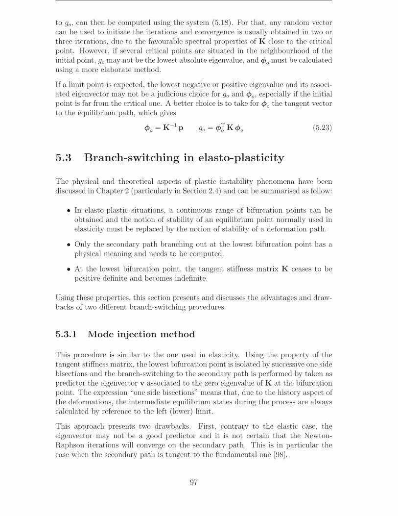
to go, can then be computed using the system (5.18). For that, any random vectorcan be used to initiate the iterations and convergence is usually obtained in two orthree iterations, due to the favourable spectral properties of K close to the criticalpoint. However, if several critical points are situated in the neighbourhood of theinitial point, go may not be the lowest absolute eigenvalue, and φo must be calculatedusing a more elaborate method.

If a limit point is expected, the lowest negative or positive eigenvalue and its associ-ated eigenvector may not be a judicious choice for go and φo, especially if the initialpoint is far from the critical one. A better choice is to take for φo the tangent vectorto the equilibrium path, which gives

φo = K−1 p go = φTo Kφo (5.23)

5.3 Branch-switching in elasto-plasticity

The physical and theoretical aspects of plastic instability phenomena have beendiscussed in Chapter 2 (particularly in Section 2.4) and can be summarised as follow:

• In elasto-plastic situations, a continuous range of bifurcation points can beobtained and the notion of stability of an equilibrium point normally used inelasticity must be replaced by the notion of stability of a deformation path.

• Only the secondary path branching out at the lowest bifurcation point has aphysical meaning and needs to be computed.

• At the lowest bifurcation point, the tangent stiffness matrix K ceases to bepositive definite and becomes indefinite.

Using these properties, this section presents and discusses the advantages and draw-backs of two different branch-switching procedures.

5.3.1 Mode injection method

This procedure is similar to the one used in elasticity. Using the property of thetangent stiffness matrix, the lowest bifurcation point is isolated by successive one sidebisections and the branch-switching to the secondary path is performed by taken aspredictor the eigenvector v associated to the zero eigenvalue of K at the bifurcationpoint. The expression “one side bisections” means that, due to the history aspect ofthe deformations, the intermediate equilibrium states during the process are alwayscalculated by reference to the left (lower) limit.

This approach presents two drawbacks. First, contrary to the elastic case, theeigenvector may not be a good predictor and it is not certain that the Newton-Raphson iterations will converge on the secondary path. This is in particular thecase when the secondary path is tangent to the fundamental one [98].

97

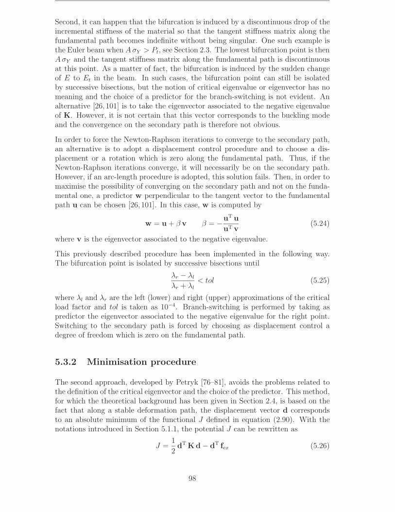
Second, it can happen that the bifurcation is induced by a discontinuous drop of theincremental stiffness of the material so that the tangent stiffness matrix along thefundamental path becomes indefinite without being singular. One such example isthe Euler beam when AσY > Pt, see Section 2.3. The lowest bifurcation point is thenAσY and the tangent stiffness matrix along the fundamental path is discontinuousat this point. As a matter of fact, the bifurcation is induced by the sudden changeof E to Et in the beam. In such cases, the bifurcation point can still be isolatedby successive bisections, but the notion of critical eigenvalue or eigenvector has nomeaning and the choice of a predictor for the branch-switching is not evident. Analternative [26, 101] is to take the eigenvector associated to the negative eigenvalueof K. However, it is not certain that this vector corresponds to the buckling modeand the convergence on the secondary path is therefore not obvious.

In order to force the Newton-Raphson iterations to converge to the secondary path,an alternative is to adopt a displacement control procedure and to choose a dis-placement or a rotation which is zero along the fundamental path. Thus, if theNewton-Raphson iterations converge, it will necessarily be on the secondary path.However, if an arc-length procedure is adopted, this solution fails. Then, in order tomaximise the possibility of converging on the secondary path and not on the funda-mental one, a predictor w perpendicular to the tangent vector to the fundamentalpath u can be chosen [26,101]. In this case, w is computed by

w = u + β v β = −uT u

uT v(5.24)

where v is the eigenvector associated to the negative eigenvalue.

This previously described procedure has been implemented in the following way.The bifurcation point is isolated by successive bisections until

λr − λl

λr + λl

< tol (5.25)

where λl and λr are the left (lower) and right (upper) approximations of the criticalload factor and tol is taken as 10−4. Branch-switching is performed by taking aspredictor the eigenvector associated to the negative eigenvalue for the right point.Switching to the secondary path is forced by choosing as displacement control adegree of freedom which is zero on the fundamental path.

5.3.2 Minimisation procedure

The second approach, developed by Petryk [76–81], avoids the problems related tothe definition of the critical eigenvector and the choice of the predictor. This method,for which the theoretical background has been given in Section 2.4, is based on thefact that along a stable deformation path, the displacement vector d correspondsto an absolute minimum of the functional J defined in equation (2.90). With thenotations introduced in Section 5.1.1, the potential J can be rewritten as

J =1

2dT Kd − dT fex (5.26)

98

Using this property, the branch-switching procedure is performed by finding anincremental solution to the equilibrium equations (5.3) which minimises J . Thus, theunstable fundamental path is rejected and the stable secondary path is automaticallyselected. This method is therefore based on the implicit assumption that, at leastin a neighbourhood of the critical point, the post-buckling path is stable.

The bifurcation point is detected and isolated by classical one side bisections. Infact, the isolation is not essential for this method. However, due to the historicalaspect of plastic deformations, it is important to initiate the secondary path from apoint which is close to the bifurcation point. The first point of the secondary pathis computed by minimising J . In order to ensure that the minimisation procedurewill not terminate on a saddle point corresponding to the fundamental path, thepredictor is constructed by adding a perturbation vector to the tangent vector atthe fundamental path u. Any random perturbation vector can be taken. However,if an eigenvalue analysis has already been performed at the bifurcation point, it canbe judicious to take the eigenvector v associated to the negative eigenvalue of K.In that case, the predictor w is computed by

w = u + αv α =1

100

‖u‖‖v‖ (5.27)

The minimisation procedure which has been implemented [36] consists of solving ateach iteration k the system

(K(k) + β I) ∆d = −r(k) (5.28)

where r is the residual vector of the equilibrium equations and I the identity matrix.The coefficient β is taken to 0 if K is positive definite and to 1.1 λmin otherwise (λmin

is the lowest eigenvalue of K). The displacements are then updated by

d(k+1) = d(k) + µ ∆d (5.29)

where µ is calculated by a line search procedure [57]. However, the tests performedby the author have shown that the line search procedure was not essential and thatµ = 1 could be taken without affecting the convergence property of the procedure.

The following points along the secondary path are then computed by classicalNewton-Raphson iterations under displacement control.

As already pointed out, this minimisation procedure assumes that the bifurcation isstable and is therefore not suited for elastic problems. For elasto-plastic instabilityproblems where buckling is induced by compressive forces, material non-linearityprevails over the geometric one in the vicinity of the bifurcation point and a stablepost-buckling path is usually observed (cf. the study of the Hutchinson’s model inSection 2.1.2). However, there is no guarantee that this is always the case. Asan example, unstable secondary path can be obtained if materials with very lowhardening are used. It can also happen that the stable region of the secondary pathis restricted to a small neighbourhood of the bifurcation point and thus is difficultto catch numerically. All these cases will be illustrated by numerical applications inChapters 6 and 9.

99

Chapter 6

2D examples in elasto-plasticity

Three main objectives motivate the selection of the numerical examples includedin this chapter. The first one is to verify the ability of the element formulationsintroduced in Chapter 3 in handling large displacement problems in the presence ofmaterial non-linearity. Two classical problems, widely used as benchmark tests inthe literature, have been chosen for this purpose. These are a cantilever beam undertip load and Lee’s frame.

The second objective of these examples is to test the two branch-switching proce-dures presented in Section 5.3 and to compute elasto-plastic post-bifurcation pathsfor structures exhibiting different types of instabilities in elasticity. Thus, the third,fourth and fifth examples are characterised in elasticity by symmetric stable, asym-metric and symmetric unstable bifurcations, respectively.

For these three examples, both the minimisation procedure and the mode injectionmethod worked very well and convergence to the first point on the secondary pathwas obtained within 4–7 iterations. However, as expected, the minimisation proce-dure failed for the case in the third example which presents an unstable bifurcation.

The third objective of these numerical applications is to examine comparatively thethree local element formulations, and especially test the differences between the twoBernoulli elements. In addition, the influence of the number of Gauss points inthe cross-section is also analysed. All these comparisons are performed through thestudy of the three first examples.

6.1 Example 1: cantilever beam

The purpose of this classical example, described in Figure 6.1, is to test and comparethe elements based on the Bernoulli assumption. The load–displacement diagramscomputed with ten linear elements and fifteen Gauss points along the beam depthare presented in Figures 6.2 and 6.3. As shown in these figures, the results are inexcellent agreement with those obtained by Kondoh and Atluri [54].

101

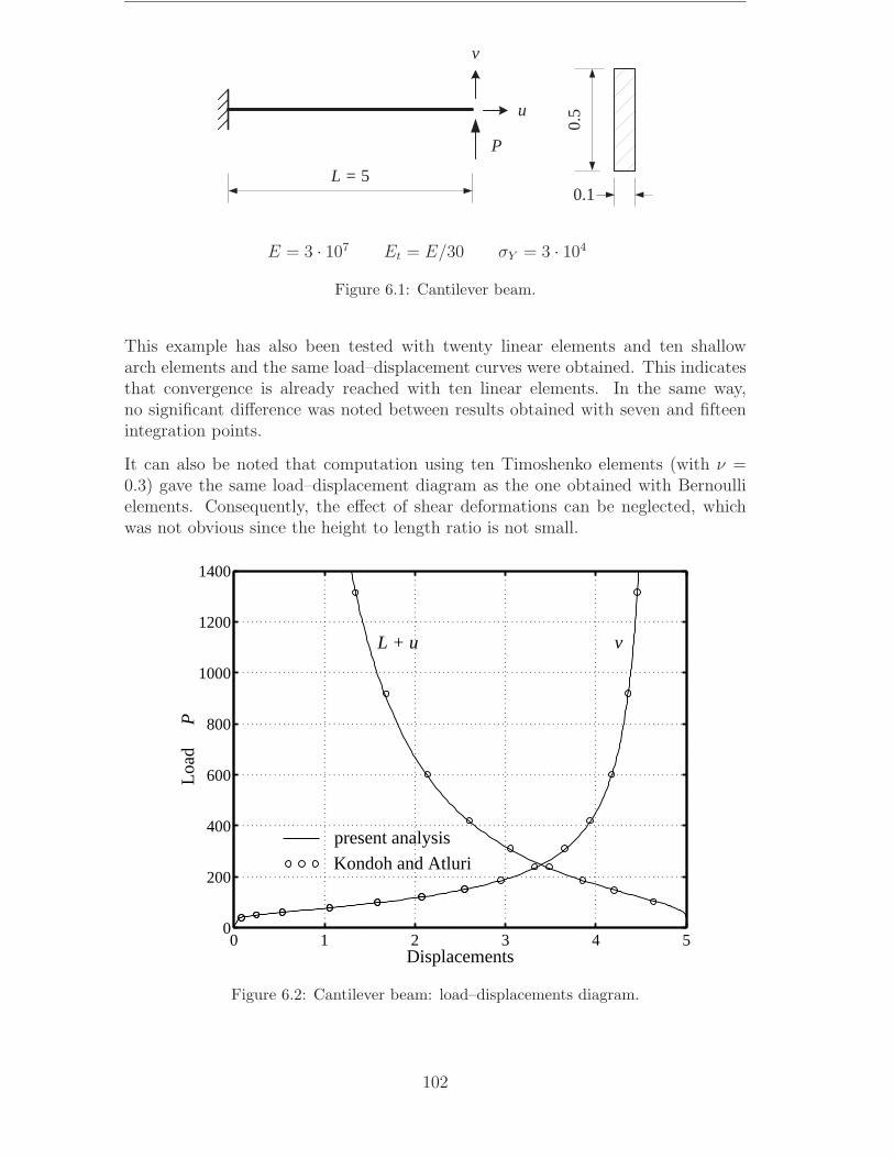
L = 5

v

u

0.

5

0.1

P

E = 3 · 107 Et = E/30 σY = 3 · 104

Figure 6.1: Cantilever beam.

This example has also been tested with twenty linear elements and ten shallowarch elements and the same load–displacement curves were obtained. This indicatesthat convergence is already reached with ten linear elements. In the same way,no significant difference was noted between results obtained with seven and fifteenintegration points.

It can also be noted that computation using ten Timoshenko elements (with ν =0.3) gave the same load–displacement diagram as the one obtained with Bernoullielements. Consequently, the effect of shear deformations can be neglected, whichwas not obvious since the height to length ratio is not small.

0 1 2 3 4 50

200

400

600

800

1000

1200

1400

Displacements

Load

P

present analysis

Kondoh and Atluri

L + u v

Figure 6.2: Cantilever beam: load–displacements diagram.

102

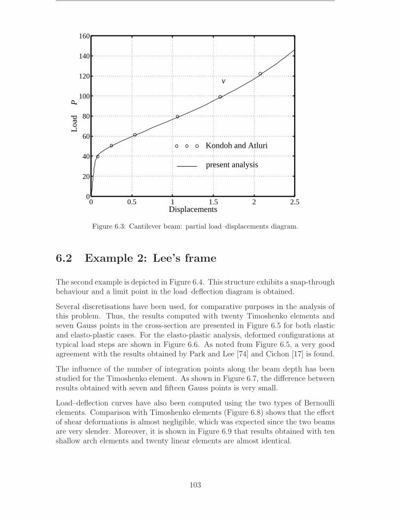
0 0.5 1 1.5 2 2.50

20

40

60

80

100

120

140

160

Displacements

Load

P

present analysis

v

Kondoh and Atluri

Figure 6.3: Cantilever beam: partial load–displacements diagram.

6.2 Example 2: Lee’s frame

The second example is depicted in Figure 6.4. This structure exhibits a snap-throughbehaviour and a limit point in the load–deflection diagram is obtained.

Several discretisations have been used, for comparative purposes in the analysis ofthis problem. Thus, the results computed with twenty Timoshenko elements andseven Gauss points in the cross-section are presented in Figure 6.5 for both elasticand elasto-plastic cases. For the elasto-plastic analysis, deformed configurations attypical load steps are shown in Figure 6.6. As noted from Figure 6.5, a very goodagreement with the results obtained by Park and Lee [74] and Cichon [17] is found.

The influence of the number of integration points along the beam depth has beenstudied for the Timoshenko element. As shown in Figure 6.7, the difference betweenresults obtained with seven and fifteen Gauss points is very small.

Load–deflection curves have also been computed using the two types of Bernoullielements. Comparison with Timoshenko elements (Figure 6.8) shows that the effectof shear deformations is almost negligible, which was expected since the two beamsare very slender. Moreover, it is shown in Figure 6.9 that results obtained with tenshallow arch elements and twenty linear elements are almost identical.

103

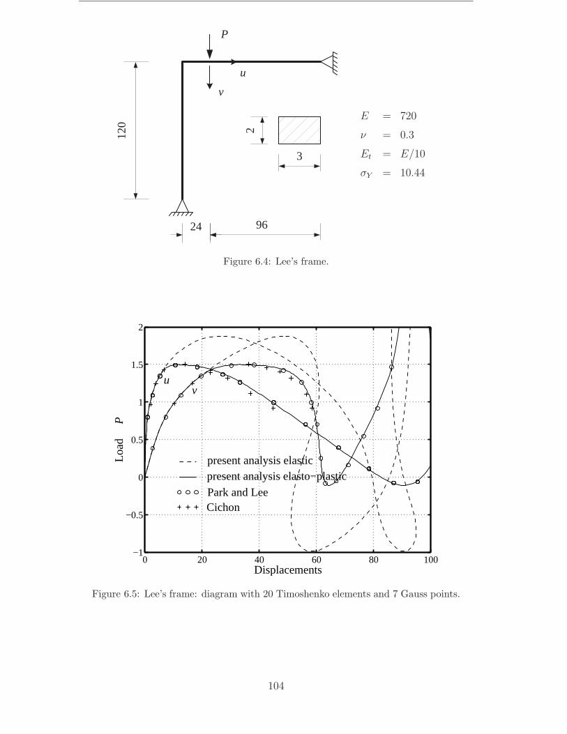
9624

P

u

v

3

2120

E = 720

ν = 0.3

Et = E/10

σY = 10.44

Figure 6.4: Lee’s frame.

0 20 40 60 80 100−1

−0.5

0

0.5

1

1.5

2

uv

Displacements

Load

P

present analysis elasticpresent analysis elasto−plastic

Park and LeeCichon

Figure 6.5: Lee’s frame: diagram with 20 Timoshenko elements and 7 Gauss points.

104

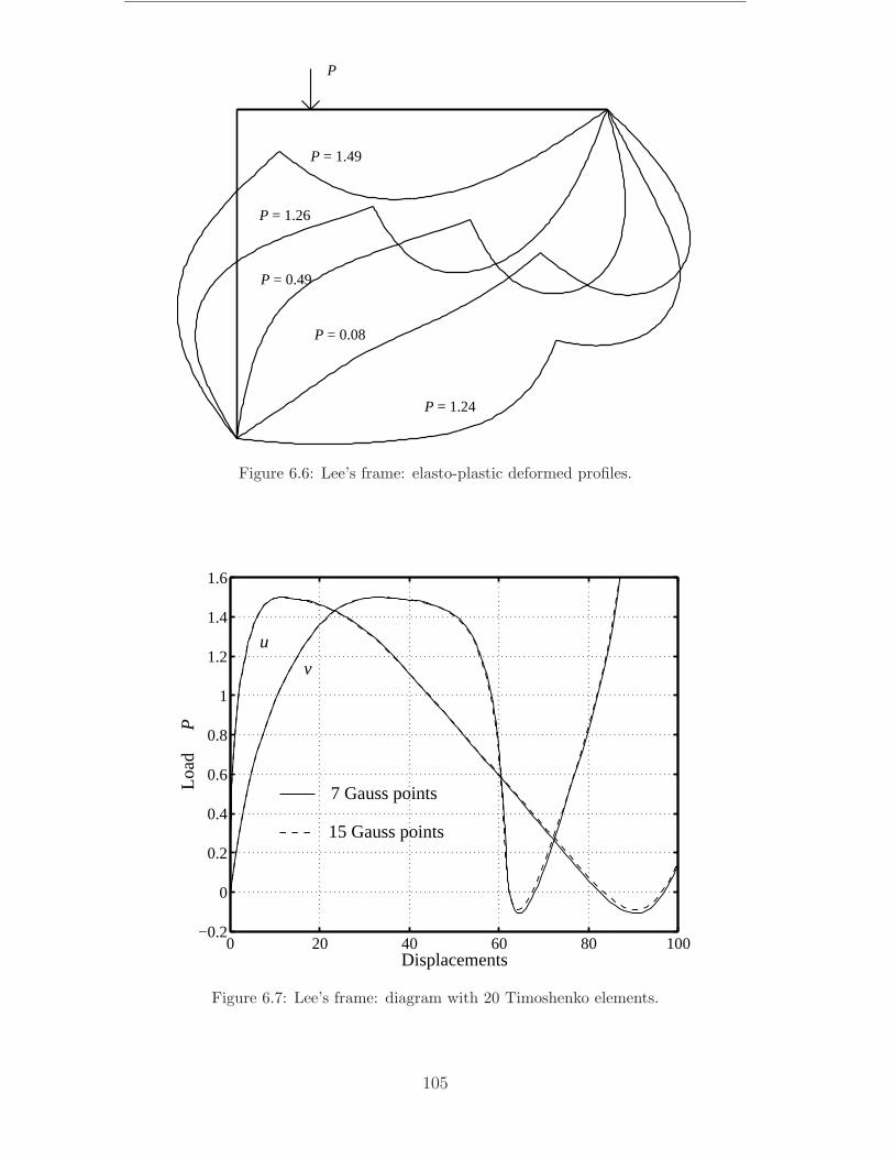
P

P = 1.49

P = 1.26

P = 0.49

P = 0.08

P = 1.24

Figure 6.6: Lee’s frame: elasto-plastic deformed profiles.

0 20 40 60 80 100−0.2

0

0.2

0.4

0.6

0.8

1

1.2

1.4

1.6

u

v

Displacements

Load

P

7 Gauss points

15 Gauss points

Figure 6.7: Lee’s frame: diagram with 20 Timoshenko elements.

105

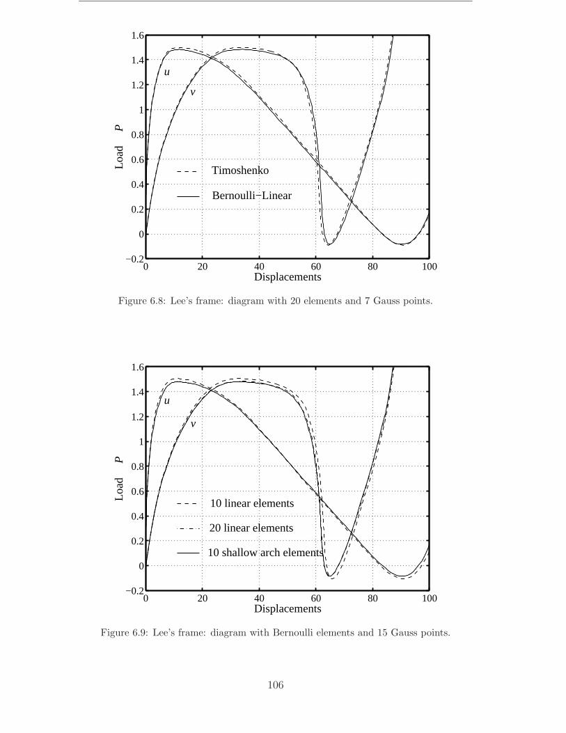
0 20 40 60 80 100−0.2

0

0.2

0.4

0.6

0.8

1

1.2

1.4

1.6

Displacements

Load

P

u

v

Timoshenko

Bernoulli−Linear

Figure 6.8: Lee’s frame: diagram with 20 elements and 7 Gauss points.

0 20 40 60 80 100−0.2

0

0.2

0.4

0.6

0.8

1

1.2

1.4

1.6

Displacements

Load

P

u

v

10 linear elements

20 linear elements

10 shallow arch elements

Figure 6.9: Lee’s frame: diagram with Bernoulli elements and 15 Gauss points.

106

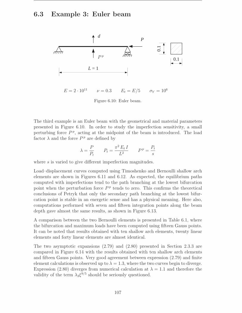
6.3 Example 3: Euler beam

L = 1

d

0.1

0.1

P

P p

E = 2 · 1011 ν = 0.3 Et = E/5 σY = 106

Figure 6.10: Euler beam.

The third example is an Euler beam with the geometrical and material parameterspresented in Figure 6.10. In order to study the imperfection sensitivity, a smallperturbing force P p, acting at the midpoint of the beam is introduced. The loadfactor λ and the force P p are defined by

λ =P

Pt

Pt =π2 Et I

L2P p =

Pt

s

where s is varied to give different imperfection magnitudes.

Load–displacement curves computed using Timoshenko and Bernoulli shallow archelements are shown in Figures 6.11 and 6.12. As expected, the equilibrium pathscomputed with imperfections tend to the path branching at the lowest bifurcationpoint when the perturbation force P p tends to zero. This confirms the theoreticalconclusions of Petryk that only the secondary path branching at the lowest bifur-cation point is stable in an energetic sense and has a physical meaning. Here also,computations performed with seven and fifteen integration points along the beamdepth gave almost the same results, as shown in Figure 6.13.

A comparison between the two Bernoulli elements is presented in Table 6.1, wherethe bifurcation and maximum loads have been computed using fifteen Gauss points.It can be noted that results obtained with ten shallow arch elements, twenty linearelements and forty linear elements are almost identical.

The two asymptotic expansions (2.79) and (2.80) presented in Section 2.3.3 arecompared in Figure 6.14 with the results obtained with ten shallow arch elementsand fifteen Gauss points. Very good agreement between expression (2.79) and finiteelement calculations is observed up to λ = 1.3, where the two curves begin to diverge.Expression (2.80) diverges from numerical calculation at λ = 1.1 and therefore thevalidity of the term λ3ξ

9/5 should be seriously questioned.

107

A number of reasons why asymptotic expressions should be considered with greatcaution have already been discussed in Section 2.3.3. The examination of the growingzone of elastic unloading, which appears at bifurcation, gives an additional argument.The zones of elastic deformations at several increments are shown in Figure 6.16.Calculations have been performed with forty shallow arch elements in order to get anaccurate representation of the zone of elastic unloading, but the load–displacementcurve is similar to the one depicted in Figure 6.14. It is shown in Figure 6.16that a zone of plastic reversal stresses is developing before the occurrence of themaximal load. This zone is not considered in the derivation of the asymptoticexpansions [49, 58]. The same phenomenon has been observed with different valuesfor the yield limit σY and the tangent modulus Et. Another consequence is that thecharacteristic of the hardening cannot be neglected. The present method is based onisotropic hardening. Similar computations with kinematic hardening would certainlygive different load–displacement diagrams.

Finally, the structure has been tested when Pt < AσY by taking σY = 5 · 108. Inthis case, the lowest bifurcation point is AσY and the tangent stiffness matrix alongthe fundamental path becomes negative at this point without being singular. Thesecondary paths computed with two different hardening parameters are presentedFigure 6.15. It can be observed that depending on the value of Et, the bifurcationcan be stable or unstable.

0 0.05 0.1 0.15 0.20.8

0.9

1

1.1

1.2

1.3

1.4

1.5

1.6

without imperfection

= 1000

= 10000s

s

Load

fact

or

λ

Displacement d

Figure 6.11: Euler beam: diagram with 20 Timoshenko elements and 15 G.p.

108

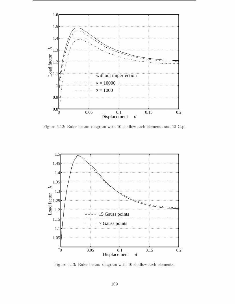
0 0.05 0.1 0.15 0.20.8

0.9

1

1.1

1.2

1.3

1.4

1.5

1.6

Displacement d

Load

fact

or

λ

without imperfection

s

s

= 10000

= 1000

Figure 6.12: Euler beam: diagram with 10 shallow arch elements and 15 G.p.

0 0.05 0.1 0.15 0.21

1.05

1.1

1.15

1.2

1.25

1.3

1.35

1.4

1.45

1.5

Displacement d

Load

fact

or

λ

15 Gauss points

7 Gauss points

Figure 6.13: Euler beam: diagram with 10 shallow arch elements.

109

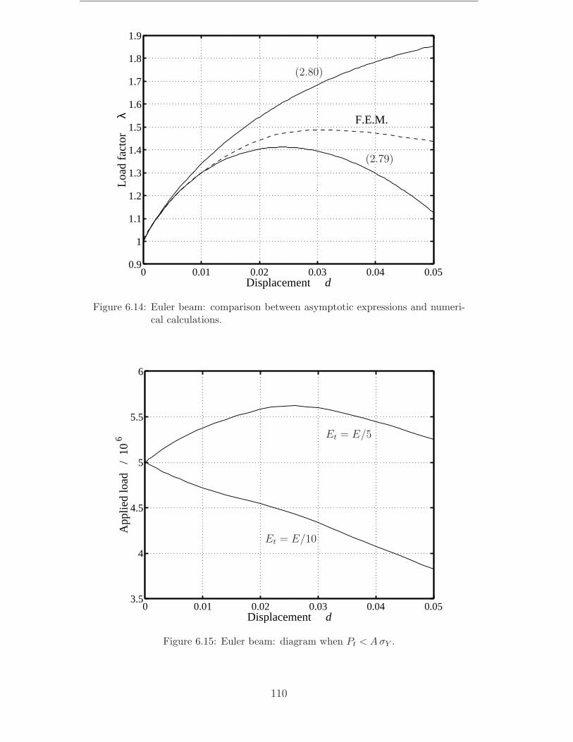
0 0.01 0.02 0.03 0.04 0.050.9

1

1.1

1.2

1.3

1.4

1.5

1.6

1.7

1.8

1.9

Displacement d

Load

fact

or

λ F.E.M.

(2.80)

(2.79)

Figure 6.14: Euler beam: comparison between asymptotic expressions and numeri-cal calculations.

0 0.01 0.02 0.03 0.04 0.053.5

4

4.5

5

5.5

6

App

lied

load

/

10 6

Displacement d

Et = E/5

Et = E/10

Figure 6.15: Euler beam: diagram when Pt < A σY .

110

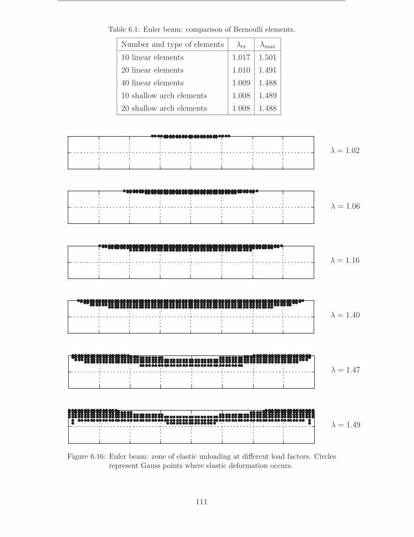
Table 6.1: Euler beam: comparison of Bernoulli elements.

Number and type of elements λcr λmax

10 linear elements 1.017 1.501

20 linear elements 1.010 1.491

40 linear elements 1.009 1.488

10 shallow arch elements 1.008 1.489

20 shallow arch elements 1.008 1.488

λ = 1.02

λ = 1.06

λ = 1.16

λ = 1.40

λ = 1.47

λ = 1.49

Figure 6.16: Euler beam: zone of elastic unloading at different load factors. Circlesrepresent Gauss points where elastic deformation occurs.

111

6.4 Example 4: asymmetrical frame

L = 1

L =

1

0.1

0.1

d

P

E = 2 · 1011

Et = E/2

σY = 106

Figure 6.17: Asymmetrical frame.

The frame described in Figure 6.17 exhibits an asymmetrical bifurcation for the caseof elastic behaviour, as shown in Figure 6.18. The load factor λ is defined by

P = λ4 π2 E I

L2in elasticity (6.1)

and

P = λ4 π2 Et I

L2in elasto-plasticity (6.2)

The purpose of this example is to investigate the phenomenon of bifurcation inelasto-plasticity. Sixteen shallow arch elements and fifteen Gauss points have beenused. The results are shown in Figure 6.19. Both post-bifurcation secondary pathspresent a stable part before a limit point is reached. These results confirm theconclusion derived from the analysis of Hutchinson’s model (Section 2.1.2) that inthe vicinity of the bifurcation, material non-linearity prevails over the geometric oneand, consequently, a stable path is usually obtained.

112

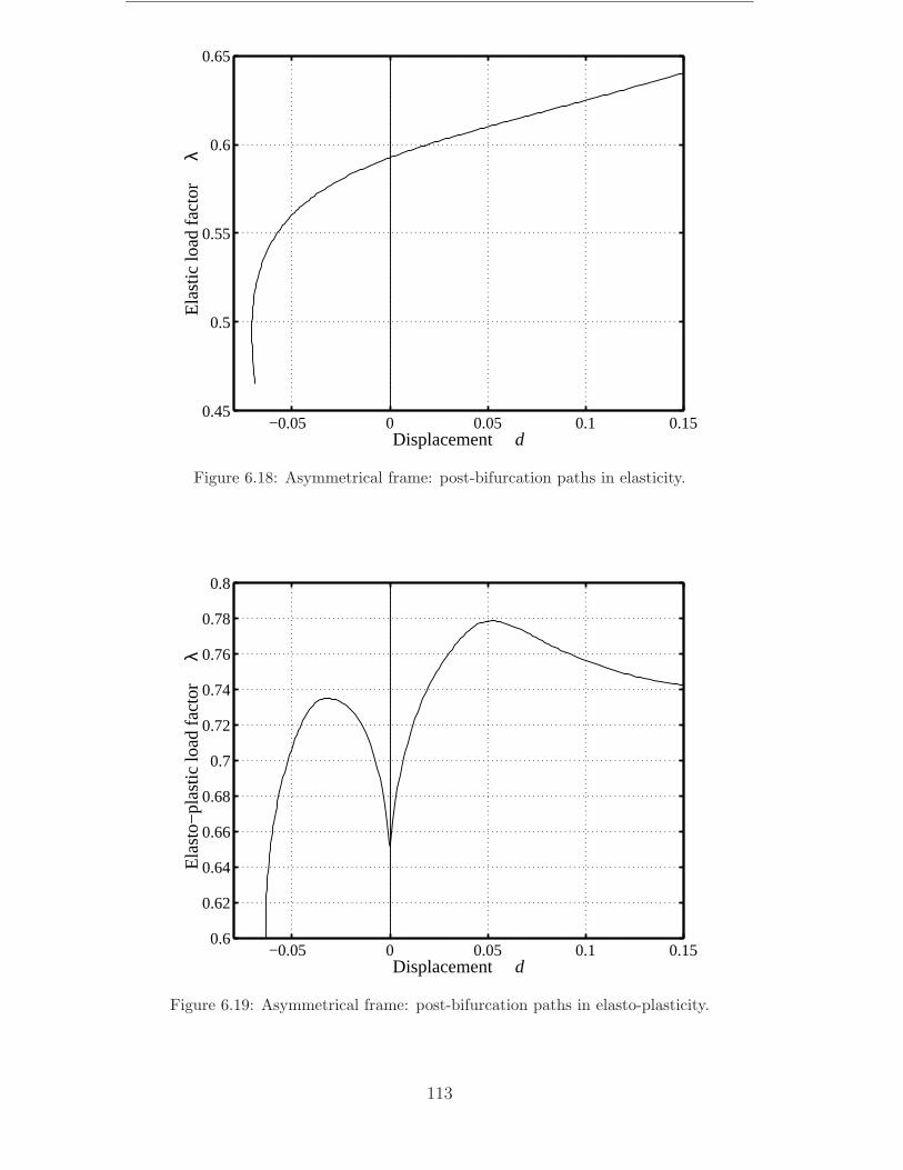
−0.05 0 0.05 0.1 0.150.45

0.5

0.55

0.6

0.65

Displacement d

Ela

stic

load

fact

or

λ

Figure 6.18: Asymmetrical frame: post-bifurcation paths in elasticity.

−0.05 0 0.05 0.1 0.150.6

0.62

0.64

0.66

0.68

0.7

0.72

0.74

0.76

0.78

0.8

Displacement d

Ela

sto−

plas

tic lo

ad fa

ctor

λ

Figure 6.19: Asymmetrical frame: post-bifurcation paths in elasto-plasticity.

113

6.5 Example 5: toggle frame

P

d

12.943 12.943

0.5 0.753

0.243

E = 107

Et = E/2

σY = 3 · 103

Figure 6.20: Toggle frame.

The toggle frame, described in Figure 6.20 has been analysed using a discretisationwith eight linear Bernoulli elements and seven Gauss points along the beam height.The equilibrium paths for the elastic and elasto-plastic situations are shown in Fig-ures 6.21 and 6.22. In the elastic case, the structure exhibits a symmetric unstablebifurcation while in the elasto-plastic case, a stable bifurcation is observed. How-ever, it must be noted that the stable part of the secondary path is very short and alimit point is quickly reached. This observation confirms once again the conclusionthat in the vicinity of the bifurcation point, material non-linearity prevails over thegeometric one and a stable path is usually obtained.

Moreover, the results plotted in Figure 6.22 suggest that the structure presents atangent bifurcation in the elasto-plastic case. The existence of such a bifurcation hasbeen proved theoretically by Leger and Potier-Ferry [58] and an example has beenstudied by Triantafyllidis [98]. According to these authors, a tangent bifurcation canoccur when the structure is only partially plasticised along the fundamental pathand is characterised by the apparition of a zone of elastic reloading. The analysis ofFigures 6.23 and 6.24 shows that along the fundamental path, a zone of plasticisationis developing on the concave side of the two beams while the rest of the structuredeforms elastically. In addition, a zone of elastic unloading (ε < 0) appears on theconvex side of the two beams. Along the secondary path, the zone of plasticisationcontinues to grow in the left beam while it decreases and disappears in the rightbeam. At the same time, the zone of elastic unloading disappears on the convexside of the right beam. Consequently, the conditions for a tangent bifurcation statedin [58] seem to be respected, but a rigorous proof of such a phenomenon cannot beperformed in a discretised and numerical context.

114

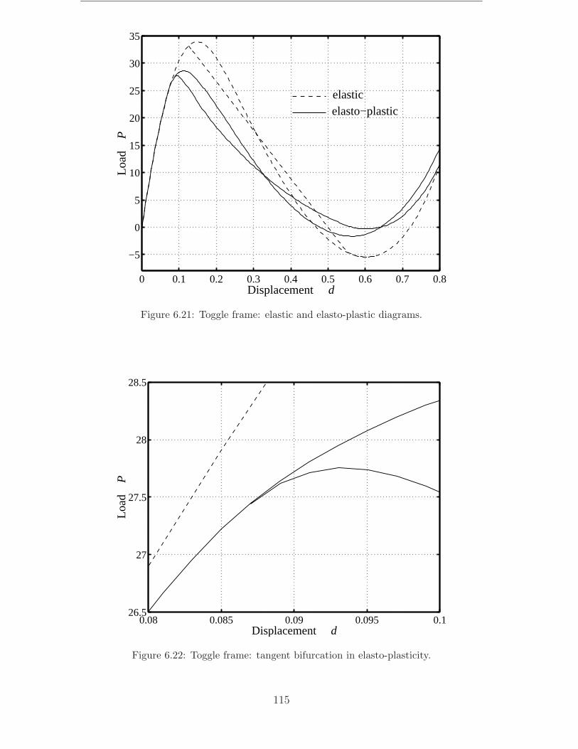
0 0.1 0.2 0.3 0.4 0.5 0.6 0.7 0.8

−5

0

5

10

15

20

25

30

35

Displacement d

Load

P

elasticelasto−plastic

Figure 6.21: Toggle frame: elastic and elasto-plastic diagrams.

0.08 0.085 0.09 0.095 0.126.5

27

27.5

28

28.5

Displacement d

Load

P

Figure 6.22: Toggle frame: tangent bifurcation in elasto-plasticity.

115

P = 27.2 d = 0.085

P = 26.9 d = 0.11

P = 18.2 d = 0.20

Figure 6.23: Toggle frame: deformed profiles before and after bifurcation.

secondary path: inc. after bifurcation secondary path: 2nd inc. after bifurcation

fundamental path: inc. before bifurcation fundamental path: inc. after bifurcation

Figure 6.24: Toggle frame: zone of plastic deformations at different increments. Cir-cles represent Gauss points where plastic deformation occurs. Starsrepresent Gauss points where elastic unloading occurs.

116

Chapter 7

3D examples in elasticity

The test problems included in this chapter have two objectives. The first one is totest the ability of the elements in handling problems involving large 3D rotations.As a general rule, the parameterisation in terms of the incremental rotation vector isused throughout the whole set of test problems. However, for the first two examples,the parameterisation based on the total rotation vector together with the moretraditional “intrinsic” parameterisation (see Section 4.2.5) were also included inorder to discuss the relative merits of the three possible choices. The second objectiveis to test the ability of the elements to deal with problems involving coupling betweenaxial, bending and torsional-warping effects. For this purpose several examplesexhibiting pure torsional or flexural-torsional buckling were also included.

For all the instability problems included in this chapter, the procedure of directisolation of bifurcation points presented in Section 5.2 was used. Convergence tothe bifurcation point was obtained within 4–6 iterations. The performances of thisprocedure will be investigated in more detail in Chapter 8.

For certain problems, the results obtained from the beam models have been com-pared with results obtained using shell models. The shell models were constructedusing the flat facet triangular element developed by Pacoste [68,71].

The characteristics of the cross-sections have been either taken from the literatureor determined with the finite element program presented in Appendix B.

7.1 Example 1, deployable ring

This first example, introduced by Goto [38], refers to the ring depicted in Figure 7.1.The ring is fully clamped at one end and loaded at the other end by a twistingmoment. At the loaded end, the center point of the section (point A) is restrictedto move along and rotate around the x axis.

117

M

A

120=R

6=h0.6=t

76923

200000

=

=

G

E

x

Figure 7.1: Deployable ring.

The ring shows a very interesting behaviour under increasing rotation at A. Thus,after a complete rotation cycle, i.e. ΘA = 2π the ring is wrapped around itself andtransformed into a smaller ring with a radius of only one third of the original one.One more cycle, i.e. ΘA = 4π, will bring the ring back to the original configuration.This example is therefore ideally suited in order to test the ability of the formulationto handle large rotations.

0 2 4 6 8 10 12−8

−6

−4

−2

0

2

4

6

8

10

Rotation at A

App

lied

mom

ent

/ 10

0

shell

rot. vec.

intrinsic

Figure 7.2: Deployable ring: load–displacement curves.

118

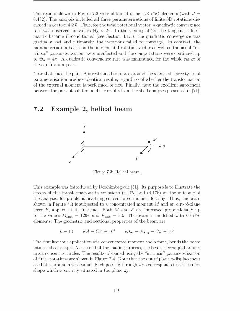
The results shown in Figure 7.2 were obtained using 128 t3dl elements (with J =0.432). The analysis included all three parameterisations of finite 3D rotations dis-cussed in Section 4.2.5. Thus, for the total rotational vector, a quadratic convergencerate was observed for values ΘA < 2π. In the vicinity of 2π, the tangent stiffnessmatrix became ill-conditioned (see Section 4.1.1), the quadratic convergence wasgradually lost and ultimately, the iterations failed to converge. In contrast, theparameterisation based on the incremental rotation vector as well as the usual “in-trinsic” parameterisation, were unaffected and the computations were continued upto ΘA = 4π. A quadratic convergence rate was maintained for the whole range ofthe equilibrium path.

Note that since the point A is restrained to rotate around the x axis, all three types ofparameterisation produce identical results, regardless of whether the transformationof the external moment is performed or not. Finally, note the excellent agreementbetween the present solution and the results from the shell analyses presented in [71].

7.2 Example 2, helical beam

x

y

zF

M

Figure 7.3: Helical beam.

This example was introduced by Ibrahimbegovic [51]. Its purpose is to illustrate theeffects of the transformations in equations (4.175) and (4.176) on the outcome ofthe analysis, for problems involving concentrated moment loading. Thus, the beamshown in Figure 7.3 is subjected to a concentrated moment M and an out-of-planeforce F , applied at its free end. Both M and F are increased proportionally upto the values Mmax = 120π and Fmax = 30. The beam is modelled with 60 t3dlelements. The geometric and sectional properties of the beam are

L = 10 EA = GA = 104 EI22 = EI33 = GJ = 102

The simultaneous application of a concentrated moment and a force, bends the beaminto a helical shape. At the end of the loading process, the beam is wrapped aroundin six concentric circles. The results, obtained using the “intrinsic” parameterisationof finite rotations are shown in Figure 7.4. Note that the out of plane z-displacementoscillates around a zero value. Each passing through zero corresponds to a deformedshape which is entirely situated in the plane xy.

119

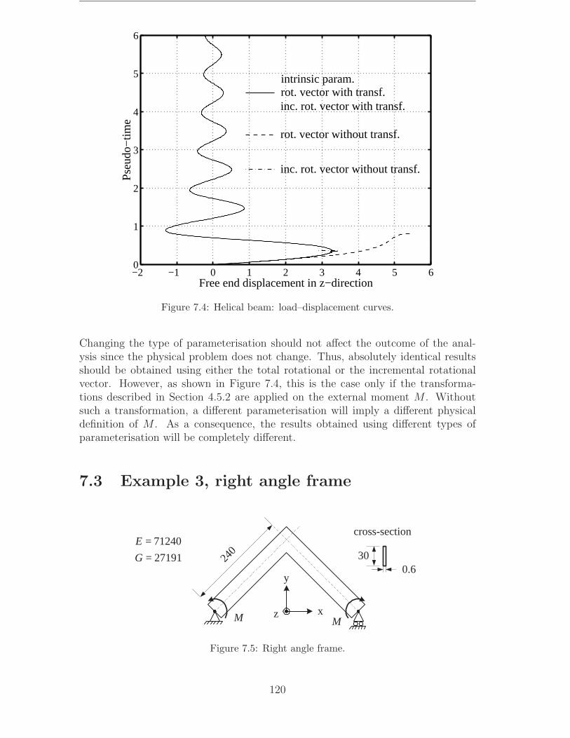
−2 −1 0 1 2 3 4 5 60

1

2

3

4

5

6

Pse

udo−

time

Free end displacement in z−direction

rot. vector with transf.inc. rot. vector with transf.

rot. vector without transf.

inc. rot. vector without transf.

intrinsic param.

Figure 7.4: Helical beam: load–displacement curves.

Changing the type of parameterisation should not affect the outcome of the anal-ysis since the physical problem does not change. Thus, absolutely identical resultsshould be obtained using either the total rotational or the incremental rotationalvector. However, as shown in Figure 7.4, this is the case only if the transforma-tions described in Section 4.5.2 are applied on the external moment M . Withoutsuch a transformation, a different parameterisation will imply a different physicaldefinition of M . As a consequence, the results obtained using different types ofparameterisation will be completely different.

7.3 Example 3, right angle frame

240

x

y

zM M

27191

71240

=

=

G

E30

0.6

cross-section

Figure 7.5: Right angle frame.

120

This classical example (see Figure 7.5), has often been used in order to check theability of various beam formulations to properly account for torsional-bending cou-pling [40,44,64,73,92,93]. Due to the symmetry, only half of the frame is modelled.At the support only translation along x and rotation around z are allowed. Theloading is given by a pair of concentrated moments applied at the support. Thenon-trivial cross sectional characteristics are J = 2.133 and Iω = 40.43.

The problem is typical for situations where a local linear strain definition will lead toan incorrect solution. Thus, the results obtained using 10 t3dl elements are shownin Figure 7.6. As the moment increases, an unstable bifurcation point is reached.These results are in excellent agreement with those found in the literature [40, 44,64,73,92,93].

A qualitatively different behaviour is predicted by the models using 10 tw3d or t3delements, as shown in Figure 7.7. A stable bifurcation point is now reached at aslightly higher value of the critical moment. The secondary path loses its stability ata limit point, for a value of the moment of about 1.20Mcr. In order to confirm theseresults, the analysis was repeated using a model with 576 triangular shell elementsfor one half of the frame. A good agreement with the beam model is observed upto a value of the apex displacement of about one half of the frame height. Over thisvalue the quantitative differences are more pronounced. According to the author’sopinion, these differences originate from the very large height to thickness ratio ofthe cross-section. As a result, in the large displacement regime, the cross-sectioncan no longer be assumed as undeformable in its plane and a beam analysis is notappropriate. Finally, it can be noted that similar results were obtained by Sauer [86].

−200 −150 −100 −50 0 50 100 150 200−800

−600

−400

−200

0

200

400

600

800

App

lied

mom

ent

Apex displacement in z−direction

Nour−Omid

t3dl

Figure 7.6: Right angle frame: post-buckling behaviour; t3dl element.

121

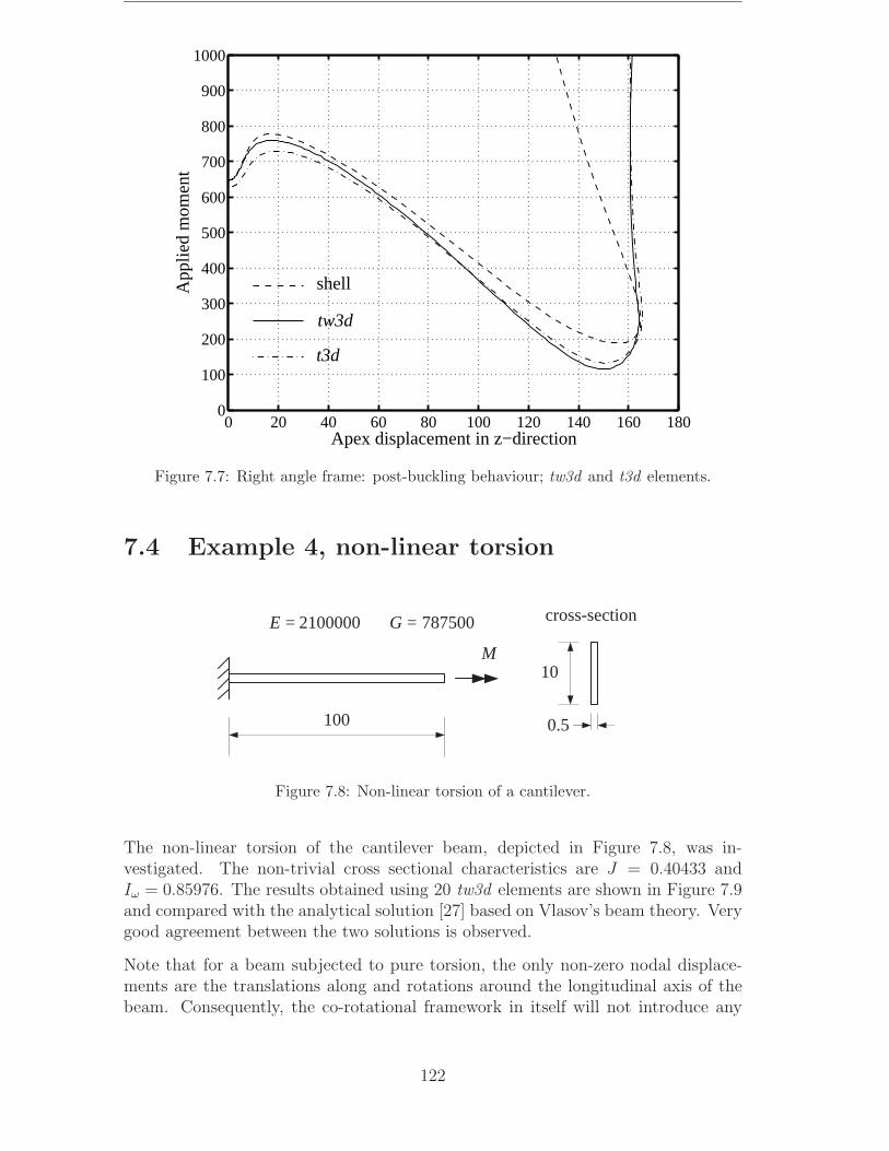
0 20 40 60 80 100 120 140 160 1800

100

200

300

400

500

600

700

800

900

1000

App

lied

mom

ent

Apex displacement in z−direction

shell

tw3d

t3d

Figure 7.7: Right angle frame: post-buckling behaviour; tw3d and t3d elements.

7.4 Example 4, non-linear torsion

M

100

7875002100000 == GE

10

cross-section

0.5

Figure 7.8: Non-linear torsion of a cantilever.

The non-linear torsion of the cantilever beam, depicted in Figure 7.8, was in-vestigated. The non-trivial cross sectional characteristics are J = 0.40433 andIω = 0.85976. The results obtained using 20 tw3d elements are shown in Figure 7.9and compared with the analytical solution [27] based on Vlasov’s beam theory. Verygood agreement between the two solutions is observed.

Note that for a beam subjected to pure torsion, the only non-zero nodal displace-ments are the translations along and rotations around the longitudinal axis of thebeam. Consequently, the co-rotational framework in itself will not introduce any

122

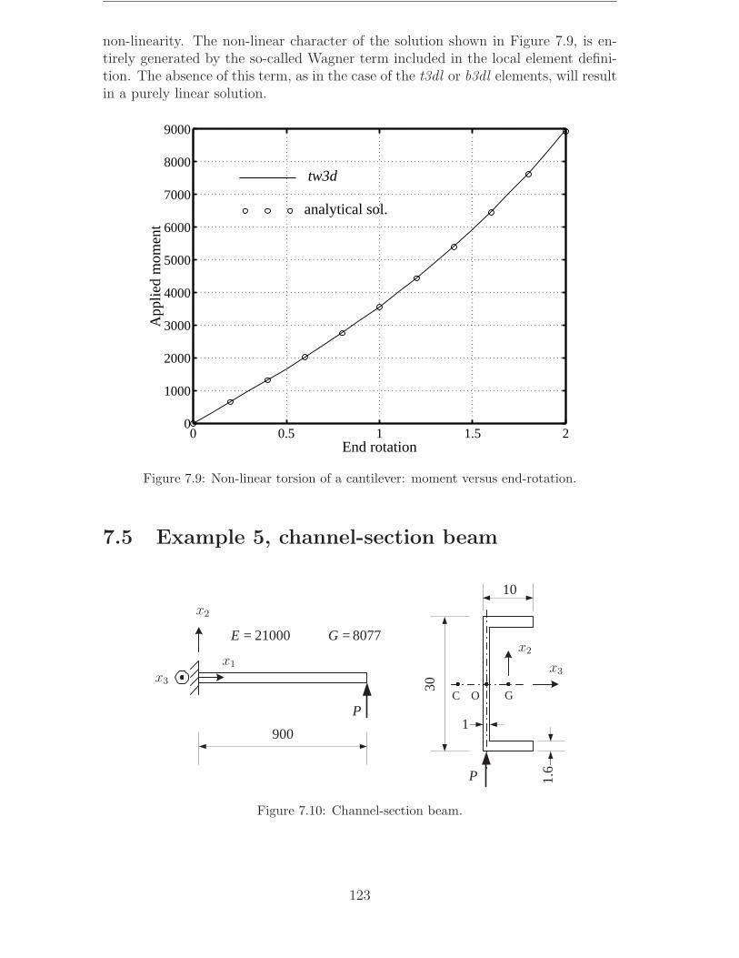
non-linearity. The non-linear character of the solution shown in Figure 7.9, is en-tirely generated by the so-called Wagner term included in the local element defini-tion. The absence of this term, as in the case of the t3dl or b3dl elements, will resultin a purely linear solution.

0 0.5 1 1.5 20

1000

2000

3000

4000

5000

6000

7000

8000

9000

App

lied

mom

ent

End rotation

tw3d

analytical sol.

Figure 7.9: Non-linear torsion of a cantilever: moment versus end-rotation.

7.5 Example 5, channel-section beam

900

P

P

GC O

30

1.6

1

10

807721000 == GE

x1

x2

x2

x3x3

Figure 7.10: Channel-section beam.

123

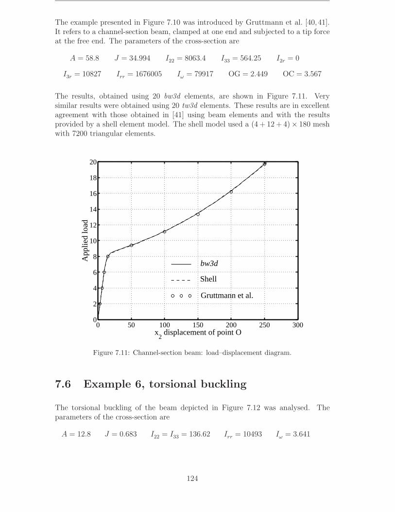
The example presented in Figure 7.10 was introduced by Gruttmann et al. [40, 41].It refers to a channel-section beam, clamped at one end and subjected to a tip forceat the free end. The parameters of the cross-section are

A = 58.8 J = 34.994 I22 = 8063.4 I33 = 564.25 I2r = 0

I3r = 10827 Irr = 1676005 Iω = 79917 OG = 2.449 OC = 3.567

The results, obtained using 20 bw3d elements, are shown in Figure 7.11. Verysimilar results were obtained using 20 tw3d elements. These results are in excellentagreement with those obtained in [41] using beam elements and with the resultsprovided by a shell element model. The shell model used a (4 + 12 + 4)× 180 meshwith 7200 triangular elements.

0 50 100 150 200 250 3000

2

4

6

8

10

12

14

16

18

20

App

lied

load

x2 displacement of point O

Shell

bw3d

Gruttmann et al.

Figure 7.11: Channel-section beam: load–displacement diagram.

7.6 Example 6, torsional buckling

The torsional buckling of the beam depicted in Figure 7.12 was analysed. Theparameters of the cross-section are

A = 12.8 J = 0.683 I22 = I33 = 136.62 Irr = 10493 Iω = 3.641

124

100

P

807721000 == GE

8

8

0.4

x2

x3

Figure 7.12: Torsional buckling.

All degrees of freedom including warping, are set to zero at the left end and onlythe axial displacement is permitted at the other end. Since the cross-section is bi-symmetrical and the axial load is applied at the centroid of the cross-section, thebending and torsional buckling modes are uncoupled.

The analysis was initiated by isolating the first three critical points on the funda-mental path of the beam. The critical modes are torsional modes with 1,2 and 3half-waves, respectively. The corresponding critical loads, obtained using a meshwith 10 bw3d elements, are listed in Table 7.1. These results are in excellent agree-ment with the analytical solutions given by Timoshenko and Gere [97] based onBernoulli beam theory with Vlasov warping. Rigorously speaking, only the bw3delement matches these assumptions. However, since for the present problem theeffects of the bending shear strains on the torsional buckling modes are negligible,the tw3d element was also included in the comparison. Note that a finer mesh oftw3d elements is needed in order to obtain the same level of accuracy as for bw3d,especially for the higher buckling modes. This situation originates from the factthat tw3d is defined using linear interpolation functions.

Table 7.1: Torsional buckling: critical loads.

No. Theory [97] 10 bw3d 10 tw3d 20 tw3d mode

1 272.57 272.57 273.55 272.80 torsional (1h-w)

2 287.35 287.38 291.99 288.40 torsional (2h-w)

3 314.99 315.17 334.00 318.89 torsional (3h-w)

Using a model with 20 bw3d elements, a post-buckling analysis was also performed.The results, plotted in Figure 7.13, are in excellent agreement with those obtainedfrom a shell model with 1600 triangular elements.

Finally note that for the present problem, an analysis using a linear local straindefinition will completely miss the torsional modes. This comes from the fact thatthe only non-zero displacements on the fundamental path are the axial ones. Insuch a situation, as also shown in example 4, the co-rotational framework does notinduce any coupling between the axial and torsional effects.

125

0 0.1 0.2 0.3 0.4 0.5 0.6200

250

300

350

400

450

500

550

600

650

700

App

lied

load

Axial rotation of the middle point

shell

bw3d

Figure 7.13: Torsional buckling: post-bifurcation behaviour.

7.7 Example 7, lateral torsional buckling

P

150

807721000 == GE

GC

10

100.2

0.2

x1

x2x2

x3

x3

Figure 7.14: Lateral torsional buckling.

This example, taken from [41], concerns the lateral torsional buckling of the beamdepicted in Figure 7.14. The characteristics of the cross-section are

A = 5.92 J = 0.0792 I22 = 110.8 I33 = 64.49 I2r = 0

I3r = 209.06 Irr = 6182.9 Iω = 1108.2 GC = 7.55

The axial load is applied at the centroid of the cross-section. The beam is assumedas simply supported. The rotation around the axis of the beam is set to zero at

126

both supports. Warping deformations are however permitted. Since the cross-section is not bi-symmetrical, both bending and torsional effects are included inthe buckling mode. The buckling loads, obtained using different discretisations arelisted in Table 7.2. Very good agreement with the theoretical solution given in [97]is obtained.

Table 7.2: Lateral torsional buckling loads.

Theory [97] 10 bw3d 10 tw3d 20 tw3d

115.54 115.62 117.18 115.81

7.8 Example 8, lateral buckling of a cantilever

P

0778

10002

=

=

G

Eh

1=t

hL 10=

Figure 7.15: Lateral buckling of a cantilever.

This example concerns the lateral buckling of the narrow rectangular cantileverbeam shown in Figure 7.15. At the free end, a transversal load is applied at thecentroid of the cross-section. The load is described as P = λPo with Po given by

Po =1

L2

√EIGJ I =

ht3

12J =

ht3

3(7.1)

The buckling loads were evaluated for various t/h ratios. The obtained bucklingload factors λcr are listed in Table 7.3. Both the b3d and b3dl elements were used inthe analysis (10 elements meshes). For comparison purposes the theoretical bucklingloads according to Timoshenko and Gere [97], are also listed in the table. Note thatfor low values of the t/h ratio, significant pre-buckling deflections occur. Varyingthis parameter will thus illustrate the influence of pre-buckling displacements on thecritical load.

Table 7.3: Lateral buckling of a cantilever: λcr for various heights h.

h Theory [97] 10 b3dl 10 b3d

50 4.013 4.039 4.039

10 4.085 4.099 4.099

5 4.324 4.313 4.314

3 5.030 5.072 5.077

127

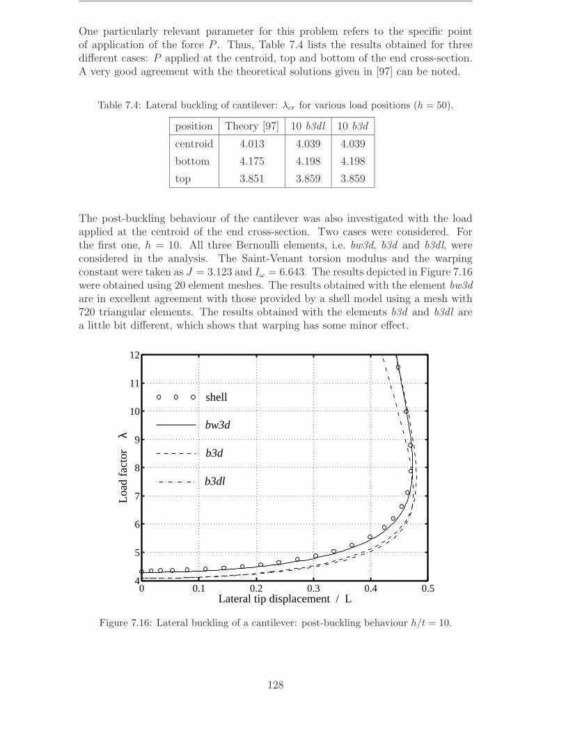
One particularly relevant parameter for this problem refers to the specific pointof application of the force P . Thus, Table 7.4 lists the results obtained for threedifferent cases: P applied at the centroid, top and bottom of the end cross-section.A very good agreement with the theoretical solutions given in [97] can be noted.

Table 7.4: Lateral buckling of cantilever: λcr for various load positions (h = 50).

position Theory [97] 10 b3dl 10 b3d

centroid 4.013 4.039 4.039

bottom 4.175 4.198 4.198

top 3.851 3.859 3.859

The post-buckling behaviour of the cantilever was also investigated with the loadapplied at the centroid of the end cross-section. Two cases were considered. Forthe first one, h = 10. All three Bernoulli elements, i.e. bw3d, b3d and b3dl, wereconsidered in the analysis. The Saint-Venant torsion modulus and the warpingconstant were taken as J = 3.123 and Iω = 6.643. The results depicted in Figure 7.16were obtained using 20 element meshes. The results obtained with the element bw3dare in excellent agreement with those provided by a shell model using a mesh with720 triangular elements. The results obtained with the elements b3d and b3dl area little bit different, which shows that warping has some minor effect.

0 0.1 0.2 0.3 0.4 0.54

5

6

7

8

9

10

11

12

shell

bw3d

b3d

b3dl

Load

fact

or

λ

Lateral tip displacement / L

Figure 7.16: Lateral buckling of a cantilever: post-buckling behaviour h/t = 10.

128

The numerical data for the second case were taken from the literature [55, 73].Referring to the notations in Figure 7.15, the following values of the geometrical,mechanical and cross-sectional parameters were used

L = 240 h = 30 t = 0.6 J = 2.133

Iω = 40.43 E = 71.24 · 106 G = 27.19 · 106

The results shown in Figure 7.17, were obtained using the same mesh and elementtypes as before. In addition, the results from a shell model with 576 triangularelements, are also plotted in the figure. For the bw3d element, good agreementwith the shell results is obtained up to a lateral displacement of about 0.45L. Thesituation is very similar to that in example 3. For very high h/t ratios, in thelarge displacement regime, a beam analysis is not appropriate due to significant in-plane deformations of the cross-section. This explanation is also supported by theresults obtained in the previous case h/t = 10 which showed an excellent agreementbetween the shell and beam models. It is worth mentioning here, that the resultsobtained using the bw3d and shell elements are significantly different from those ofKouhia [55]. According to the author’s opinion, the differences are due to the factthat in the cited reference, an averaged form of the Wagner term (see Section 4.3.2)is used in the definition of the element.

Finally note that the b3dl element (which is also used in [73]) appears to be toocrude in order to model correctly the post-buckling behaviour of the cantilever beam,especially when the ratio h/t is high.

0 0.1 0.2 0.3 0.4 0.5 0.64

5

6

7

8

9

10

Lateral tip displacement / L

Load

fact

or

λ

shell

bw3d

b3d

b3dl

Kouhia

Figure 7.17: Lateral buckling of a cantilever: post-buckling behaviour h/t = 50.

129

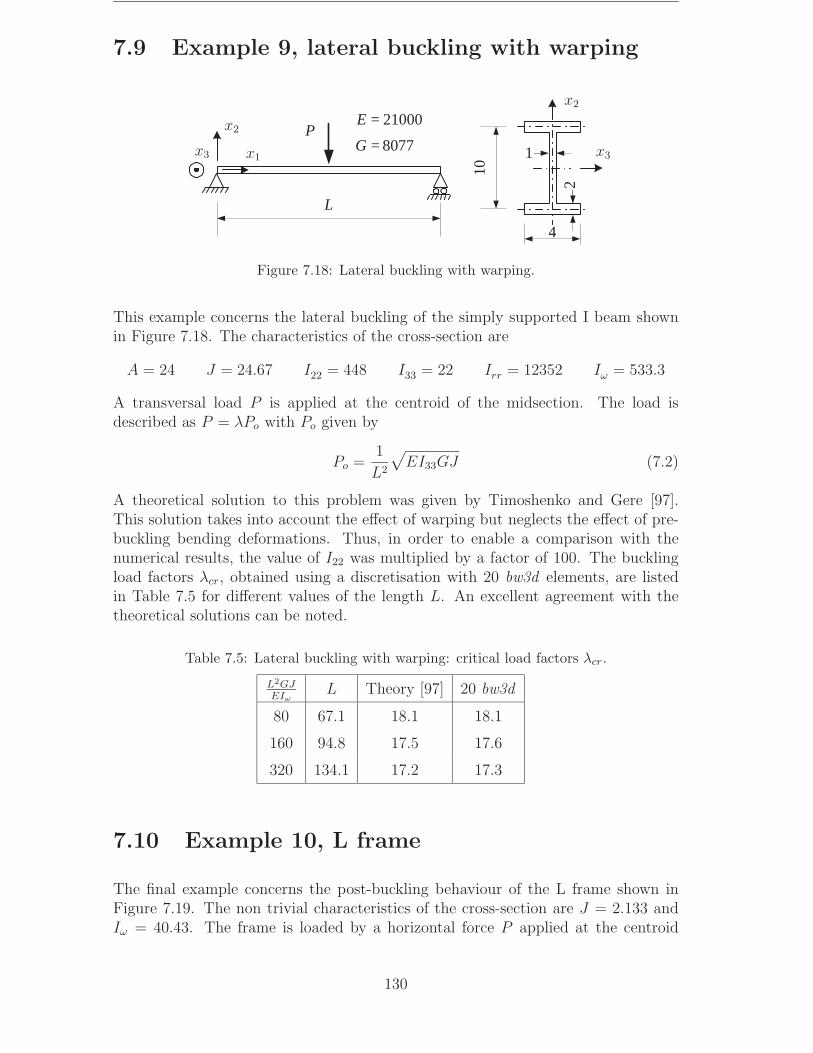
7.9 Example 9, lateral buckling with warping

P

L

8077=G

10

4

1

2

21000=E

x1

x2

x2

x3x3

Figure 7.18: Lateral buckling with warping.

This example concerns the lateral buckling of the simply supported I beam shownin Figure 7.18. The characteristics of the cross-section are

A = 24 J = 24.67 I22 = 448 I33 = 22 Irr = 12352 Iω = 533.3

A transversal load P is applied at the centroid of the midsection. The load isdescribed as P = λPo with Po given by

Po =1

L2

√EI33GJ (7.2)

A theoretical solution to this problem was given by Timoshenko and Gere [97].This solution takes into account the effect of warping but neglects the effect of pre-buckling bending deformations. Thus, in order to enable a comparison with thenumerical results, the value of I22 was multiplied by a factor of 100. The bucklingload factors λcr, obtained using a discretisation with 20 bw3d elements, are listedin Table 7.5 for different values of the length L. An excellent agreement with thetheoretical solutions can be noted.

Table 7.5: Lateral buckling with warping: critical load factors λcr.

L2GJEIω

L Theory [97] 20 bw3d

80 67.1 18.1 18.1

160 94.8 17.5 17.6

320 134.1 17.2 17.3

7.10 Example 10, L frame

The final example concerns the post-buckling behaviour of the L frame shown inFigure 7.19. The non trivial characteristics of the cross-section are J = 2.133 andIω = 40.43. The frame is loaded by a horizontal force P applied at the centroid

130

of the end cross-section. Two different modelling alternatives were tested in theanalysis. The first one disregards the finite dimensions of the connection and usesbeam elements for the whole length of the frame members. For the second one,the connection area is modelled using rigid links, as shown in Figure 7.19. In bothcases, a discretisation with 10 tw3d elements per member was used. The obtainedresults are shown in Figure 7.20. The rigid link model gives a reasonably good fitwith shell results obtained using a mesh with 512 triangular elements. Note thatthe use of rigid links amounts to assuming the connection area as infinitely rigid,which is certainly not the case. This explains the slightly overstiff behaviour of therigid link beam model.

x

y

P

255

255

A

z

cross-section

30

0.6

27191

71240

=

=

G

E

Figure 7.19: L frame.

0 10 20 30 40 50 601

1.2

1.4

1.6

1.8

2

2.2

2.4

2.6

2.8

3

shell

App

lied

load

z−displacement of point A

rigid link

model 1

Figure 7.20: L frame: post-buckling behaviour.

131

Chapter 8

Elastic isolation – examples

The purpose of the eight problems included in this chapter is to compare the per-formances of the procedure presented in Section 5.2 with the classical approach ofWriggers et al. [104, 105]. For that, the number of iterations required for conver-gence is given in tables. Note that for the present method, both the total numberof iterations and the number of the iterations which used the extended system (inparenthesis) are given. In order to allow a better comparison, for each structure,the isolation procedure was initiated from several equilibrium points.

The tolerance, tol, is given for each example. For the classical approach, this refersto the norm of the residual of the extended system. For the present method, itsdefinition is given in Table 5.3.

The 2D numerical examples were solved by using a local linear Timoshenko element,while the 3D examples were computed using the local Timoshenko element t3dpresented in Section 4.3.4.

8.1 Example 1, 2D clamped arch

145

100

F

d6

10=== EIGAEA

Figure 8.1: 2D clamped arch.

133

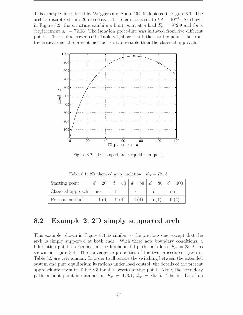
This example, introduced by Wriggers and Simo [104] is depicted in Figure 8.1. Thearch is discretised into 20 elements. The tolerance is set to tol = 10−6. As shownin Figure 8.2, the structure exhibits a limit point at a load Fcr = 972.9 and for adisplacement dcr = 72.13. The isolation procedure was initiated from five differentpoints. The results, presented in Table 8.1, show that if the starting point is far fromthe critical one, the present method is more reliable than the classical approach.

0 20 40 60 80 100 1200

100

200

300

400

500

600

700

800

900

1000Lo

ad

F

Displacement d

Figure 8.2: 2D clamped arch: equilibrium path.

Table 8.1: 2D clamped arch: isolation – dcr = 72.13

Starting point d = 20 d = 40 d = 60 d = 80 d = 100

Classical approach no 8 5 5 no

Present method 11 (6) 9 (4) 6 (4) 5 (4) 9 (4)

8.2 Example 2, 2D simply supported arch

This example, shown in Figure 8.3, is similar to the previous one, except that thearch is simply supported at both ends. With these new boundary conditions, abifurcation point is obtained on the fundamental path for a force Fcr = 334.9, asshown in Figure 8.4. The convergence properties of the two procedures, given inTable 8.2 are very similar. In order to illustrate the switching between the extendedsystem and pure equilibrium iterations under load control, the details of the presentapproach are given in Table 8.3 for the lowest starting point. Along the secondarypath, a limit point is obtained at Fcr = 423.1, dcr = 86.65. The results of its

134

isolation, presented in Table 8.4, show that the present method is better if thestarting point is far from the limit one.

145

100

F

d6

10=== EIGAEA

Figure 8.3: 2D simply supported arch.

0 20 40 60 80 1000

100

200

300

400

500

600

Load

F

Displacement d

Figure 8.4: 2D simply supported arch: equilibrium paths.

Table 8.2: 2D simply supported arch: isolation of the bifurcation pt – Fcr = 334.9

Starting point F = 200 F = 300 F = 400 F = 500

Classical approach 5 4 5 6

Present method 6 (4) 4 (3) 6 (3) 7 (4)

135

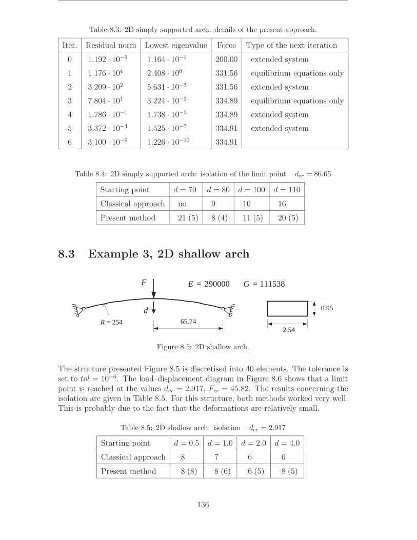
Table 8.3: 2D simply supported arch: details of the present approach.

Iter. Residual norm Lowest eigenvalue Force Type of the next iteration

0 1.192 · 10−9 1.164 · 10−1 200.00 extended system

1 1.176 · 104 2.408 · 100 331.56 equilibrium equations only

2 3.209 · 102 5.631 · 10−3 331.56 extended system

3 7.804 · 101 3.224 · 10−2 334.89 equilibrium equations only

4 1.786 · 10−1 1.738 · 10−5 334.89 extended system

5 3.372 · 10−4 1.525 · 10−7 334.91 extended system

6 3.100 · 10−9 1.226 · 10−10 334.91

Table 8.4: 2D simply supported arch: isolation of the limit point – dcr = 86.65

Starting point d = 70 d = 80 d = 100 d = 110

Classical approach no 9 10 16

Present method 21 (5) 8 (4) 11 (5) 20 (5)

8.3 Example 3, 2D shallow arch

F

dR = 254 65.74

2.54

0.95

111538290000 == GE

Figure 8.5: 2D shallow arch.

The structure presented Figure 8.5 is discretised into 40 elements. The tolerance isset to tol = 10−6. The load–displacement diagram in Figure 8.6 shows that a limitpoint is reached at the values dcr = 2.917, Fcr = 45.82. The results concerning theisolation are given in Table 8.5. For this structure, both methods worked very well.This is probably due to the fact that the deformations are relatively small.

Table 8.5: 2D shallow arch: isolation – dcr = 2.917

Starting point d = 0.5 d = 1.0 d = 2.0 d = 4.0

Classical approach 8 7 6 6

Present method 8 (8) 8 (6) 6 (5) 8 (5)

136

0 1 2 3 4 50

5

10

15

20

25

30

35

40

45

50

Load

F

Displacement d

Figure 8.6: 2D shallow arch: equilibrium path.

8.4 Example 4, deep circular arch

145

100

F

d

6

6

103

106

=

=

G

E

Figure 8.7: Deep circular arch.

This example, shown in Figure 8.7 has been introduced by Cardona and Huespe [12].The arch is fully clamped at one end and only the in plane rotation is permitted atthe other end. The tolerance is set to tol = 10−6. The structure is discretised using40 elements. The characteristics of the square cross-section are

A = 1.414 I22 = I33 = 0.1667 J = 0.4741 Irr = 0.1100

The structure (see Figure 8.8) presents a bifurcation point at a load value Fcr =256.7, corresponding to an out of plane bifurcation mode. For this problem (seeTable 8.6), both isolation methods give almost similar results.

137

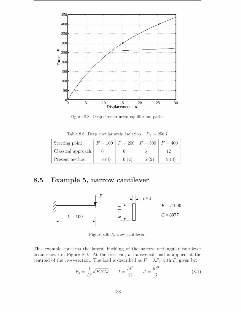
0 5 10 15 20 25 300

50

100

150

200

250

300

350

400

450

For

ce

F

Displacement d

Figure 8.8: Deep circular arch: equilibrium paths.

Table 8.6: Deep circular arch: isolation – Fcr = 256.7

Starting point F = 100 F = 200 F = 300 F = 400

Classical approach 6 6 6 12

Present method 8 (4) 6 (2) 6 (2) 9 (3)

8.5 Example 5, narrow cantilever

F

L = 100

1=t

h =

10

0778

10002

=

=

G

E

Figure 8.9: Narrow cantilever.

This example concerns the lateral buckling of the narrow rectangular cantileverbeam shown in Figure 8.9. At the free end, a transversal load is applied at thecentroid of the cross-section. The load is described as F = λFo with Fo given by:

Fo =1

L2

√EIGJ I =

ht3

12J =

ht3

3(8.1)

138

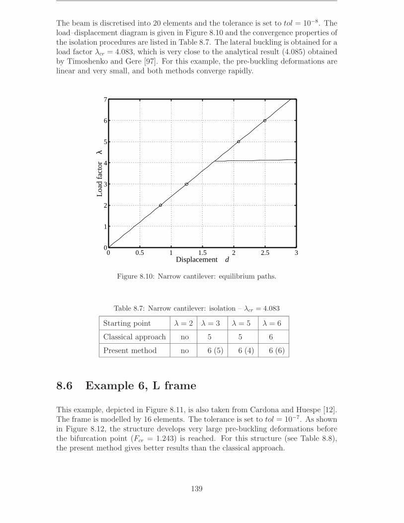
The beam is discretised into 20 elements and the tolerance is set to tol = 10−8. Theload–displacement diagram is given in Figure 8.10 and the convergence properties ofthe isolation procedures are listed in Table 8.7. The lateral buckling is obtained for aload factor λcr = 4.083, which is very close to the analytical result (4.085) obtainedby Timoshenko and Gere [97]. For this example, the pre-buckling deformations arelinear and very small, and both methods converge rapidly.

0 0.5 1 1.5 2 2.5 30

1

2

3

4

5

6

7Lo

ad fa

ctor

λ

Displacement d

Figure 8.10: Narrow cantilever: equilibrium paths.

Table 8.7: Narrow cantilever: isolation – λcr = 4.083

Starting point λ = 2 λ = 3 λ = 5 λ = 6

Classical approach no 5 5 6

Present method no 6 (5) 6 (4) 6 (6)

8.6 Example 6, L frame

This example, depicted in Figure 8.11, is also taken from Cardona and Huespe [12].The frame is modelled by 16 elements. The tolerance is set to tol = 10−7. As shownin Figure 8.12, the structure develops very large pre-buckling deformations beforethe bifurcation point (Fcr = 1.243) is reached. For this structure (see Table 8.8),the present method gives better results than the classical approach.

139

F d

240

240

cross-section

3.5

1.2

27191

71240

=

=

G

E

Figure 8.11: L frame.

0 20 40 60 80 100 1200

0.5

1

1.5

2

2.5

For

ce

F

Displacement d

Figure 8.12: L frame: equilibrium paths.

Table 8.8: L frame: isolation – Fcr = 1.243

Starting point F = 0.7 F = 1.0 F = 1.5 F = 2.0

Classical approach no 21 7 13

Present method no 6 (3) 6 (3) 8 (4)

140

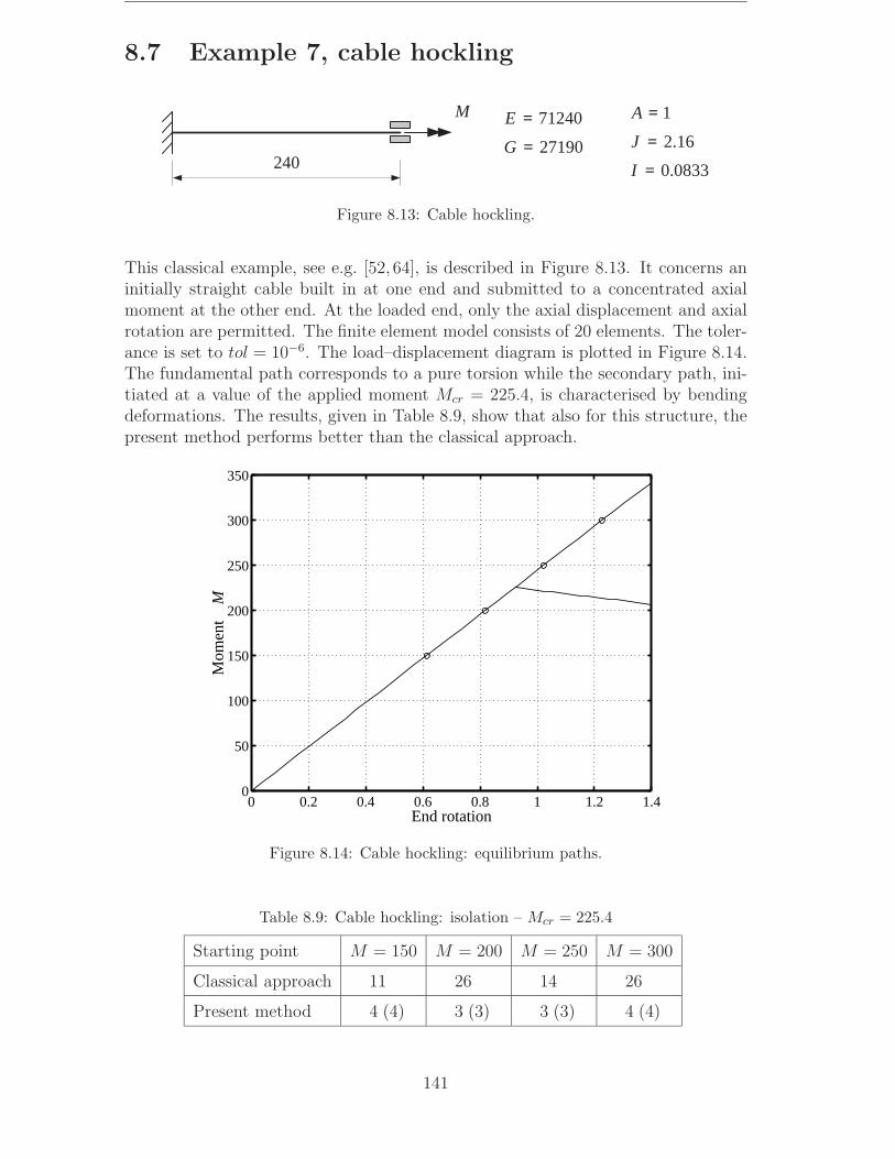
8.7 Example 7, cable hockling

M

24027190

71240

=

=

G

E

0.0833

2.16

1

=

=

=

I

J

A

Figure 8.13: Cable hockling.

This classical example, see e.g. [52, 64], is described in Figure 8.13. It concerns aninitially straight cable built in at one end and submitted to a concentrated axialmoment at the other end. At the loaded end, only the axial displacement and axialrotation are permitted. The finite element model consists of 20 elements. The toler-ance is set to tol = 10−6. The load–displacement diagram is plotted in Figure 8.14.The fundamental path corresponds to a pure torsion while the secondary path, ini-tiated at a value of the applied moment Mcr = 225.4, is characterised by bendingdeformations. The results, given in Table 8.9, show that also for this structure, thepresent method performs better than the classical approach.

0 0.2 0.4 0.6 0.8 1 1.2 1.40

50

100

150

200

250

300

350

Mom

ent

M

End rotation

Figure 8.14: Cable hockling: equilibrium paths.

Table 8.9: Cable hockling: isolation – Mcr = 225.4

Starting point M = 150 M = 200 M = 250 M = 300

Classical approach 11 26 14 26

Present method 4 (4) 3 (3) 3 (3) 4 (4)

141

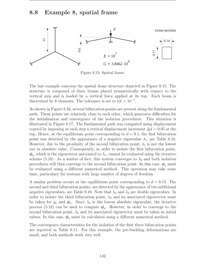
8.8 Example 8, spatial frame

15

0.6

F

0.17

0.14

cross-section

6

7

103.8462

10

=

=

G

E

Figure 8.15: Spatial frame.

The last example concerns the spatial dome structure depicted in Figure 8.15. Thestructure is composed of three beams placed symmetrically with respect to thevertical axis and is loaded by a vertical force applied at its top. Each beam isdiscretised by 8 elements. The tolerance is set to tol = 10−7.

As shown in Figure 8.16, several bifurcation points are present along the fundamentalpath. These points are relatively close to each other, which generates difficulties forthe initialisation and convergence of the isolation procedures. This situation isillustrated in Figure 8.17. The fundamental path was computed using displacementcontrol by imposing at each step a vertical displacement increment ∆d = 0.05 at thetop. Hence, at the equilibrium point corresponding to d = 0.1, the first bifurcationpoint was detected by the appearance of a negative eigenvalue λ1, see Table 8.10.However, due to the proximity of the second bifurcation point, λ1 is not the lowestone in absolute value. Consequently, in order to isolate the first bifurcation point,φo, which is the eigenvector associated to λ1, cannot be evaluated using the iterativescheme (5.18). As a matter of fact, this system converges to λ2 and both isolationprocedures will then converge to the second bifurcation point. In this case, φo mustbe evaluated using a different numerical method. This operation may take sometime, particulary for systems with large number of degrees of freedom.

A similar problem occurs at the equilibrium point corresponding to d = 0.15. Thesecond and third bifurcation points, are detected by the appearance of two additionalnegative eigenvalues, see Table 8.10. Note that λ2 and λ3 are double eigenvalues. Inorder to isolate the third bifurcation point, λ3 and its associated eigenvector mustbe taken for go and φo. Since λ3 is the lowest absolute eigenvalue, the iterativeprocess (5.18) can be used to compute φo. However, in order to converge to thesecond bifurcation point, λ2 and its associated eigenvector must be taken as initialvalues. In this case, φo must be calculated using a different numerical method.

The convergence characteristics for the isolation of the first three bifurcation pointsare reported in Table 8.11. For this example, the pre-buckling deformations aresmall, and both methods work very well.

142

0 0.2 0.4 0.6 0.8 1−1

0

1

2

3

4

5

6

7

8

9

For

ce

F

Vertical displacement at the top

Figure 8.16: Spatial frame: equilibrium paths.

0 0.05 0.1 0.15 0.20

1

2

3

4

5

6

7

8

9

For

ce

F

Vertical displacement at the top

Figure 8.17: Spatial frame: near bifurcation points.

143

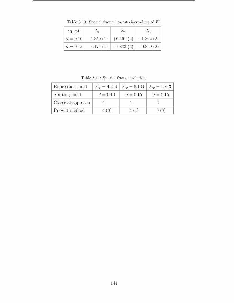
Table 8.10: Spatial frame: lowest eigenvalues of K.

eq. pt. λ1 λ2 λ3

d = 0.10 −1.850 (1) +0.191 (2) +1.892 (2)

d = 0.15 −4.174 (1) −1.883 (2) −0.359 (2)

Table 8.11: Spatial frame: isolation.

Bifurcation point Fcr = 4.249 Fcr = 6.169 Fcr = 7.313

Starting point d = 0.10 d = 0.15 d = 0.15

Classical approach 4 4 3

Present method 4 (3) 4 (4) 3 (3)

144

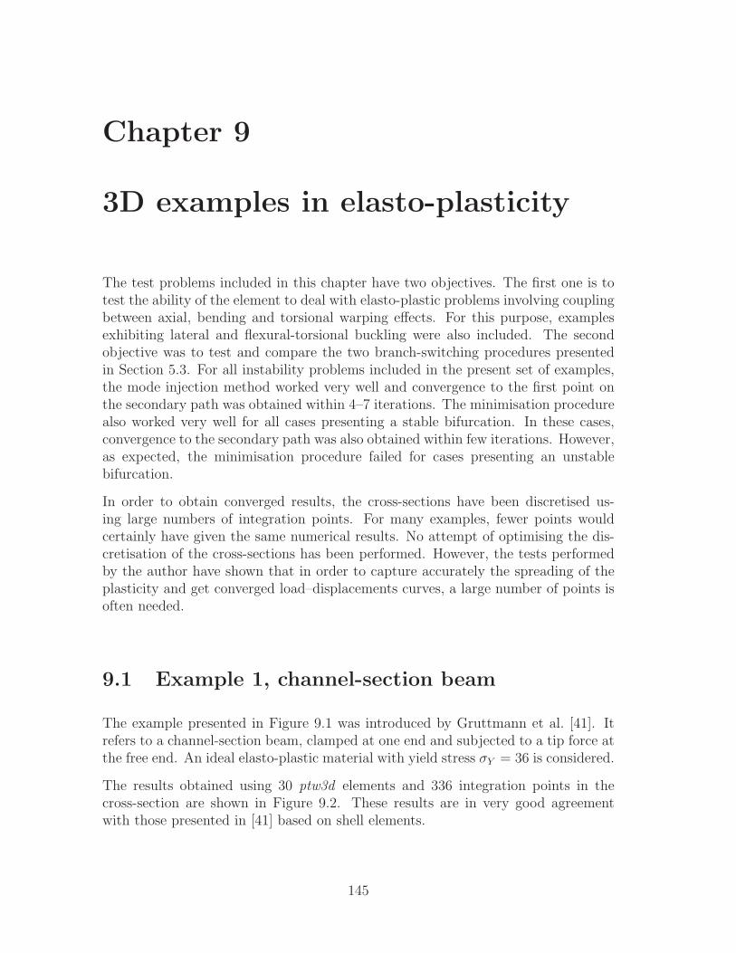
Chapter 9

3D examples in elasto-plasticity

The test problems included in this chapter have two objectives. The first one is totest the ability of the element to deal with elasto-plastic problems involving couplingbetween axial, bending and torsional warping effects. For this purpose, examplesexhibiting lateral and flexural-torsional buckling were also included. The secondobjective was to test and compare the two branch-switching procedures presentedin Section 5.3. For all instability problems included in the present set of examples,the mode injection method worked very well and convergence to the first point onthe secondary path was obtained within 4–7 iterations. The minimisation procedurealso worked very well for all cases presenting a stable bifurcation. In these cases,convergence to the secondary path was also obtained within few iterations. However,as expected, the minimisation procedure failed for cases presenting an unstablebifurcation.

In order to obtain converged results, the cross-sections have been discretised us-ing large numbers of integration points. For many examples, fewer points wouldcertainly have given the same numerical results. No attempt of optimising the dis-cretisation of the cross-sections has been performed. However, the tests performedby the author have shown that in order to capture accurately the spreading of theplasticity and get converged load–displacements curves, a large number of points isoften needed.

9.1 Example 1, channel-section beam

The example presented in Figure 9.1 was introduced by Gruttmann et al. [41]. Itrefers to a channel-section beam, clamped at one end and subjected to a tip force atthe free end. An ideal elasto-plastic material with yield stress σY = 36 is considered.

The results obtained using 30 ptw3d elements and 336 integration points in thecross-section are shown in Figure 9.2. These results are in very good agreementwith those presented in [41] based on shell elements.

145

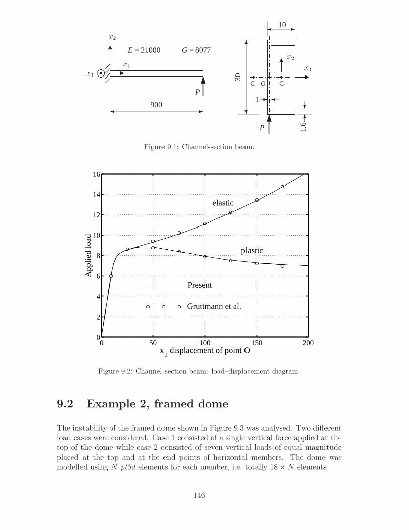
900

P

P

GC O

30

1.6

1

10

807721000 == GE

x1

x2

x2

x3x3

Figure 9.1: Channel-section beam.

0 50 100 150 2000

2

4

6

8

10

12

14

16

x2 displacement of point O

App

lied

load

elastic

plastic

Gruttmann et al.

Present

Figure 9.2: Channel-section beam: load–displacement diagram.

9.2 Example 2, framed dome

The instability of the framed dome shown in Figure 9.3 was analysed. Two differentload cases were considered. Case 1 consisted of a single vertical force applied at thetop of the dome while case 2 consisted of seven vertical loads of equal magnitudeplaced at the top and at the end points of horizontal members. The dome wasmodelled using N pt3d elements for each member, i.e. totally 18 × N elements.

146

12.57

24.38

1.22

0.76

1.55

4.55

cross-section

E = 20690 G = 8830 Et = E/5 σY = 60

Figure 9.3: Framed dome.

For the elastic material, the results computed with N = 5 and N = 8 are presentedin Figures 9.4 and 9.5. Very good agreement with Kouhia [56], who used N = 5,is observed. It can be noted that there are several bifurcation points along thefundamental paths. In Figures 9.4 and 9.5, only the fundamental path and thesecondary path branching out at the lowest bifurcation point are represented. Forboth loadings, the buckling mode is a rotation around a vertical axis, see Figure 9.6.

0 2 4 6 8 10 120

20

40

60

80

100

120

140

160

180

200

App

lied

load

Vertical displacement at the top

present N = 5present N = 8

Kouhia N = 5

Figure 9.4: Framed dome: elastic material – case 1.

147

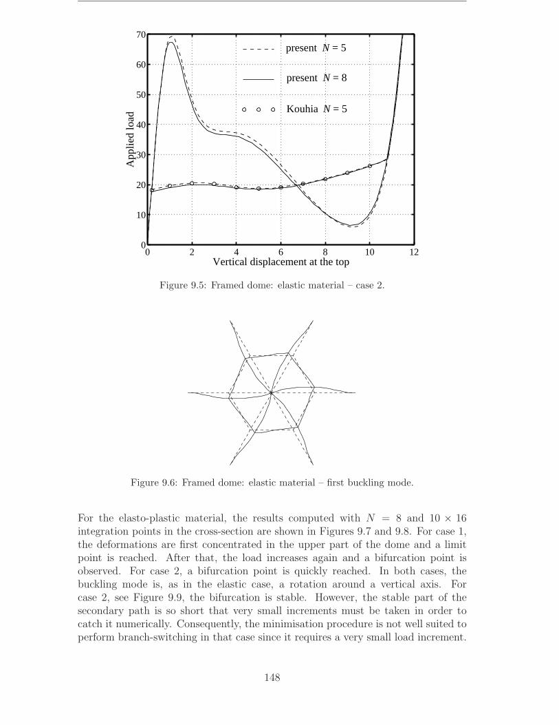
0 2 4 6 8 10 120

10

20

30

40

50

60

70

App

lied

load

Vertical displacement at the top

Kouhia N = 5

present N = 8

present N = 5

Figure 9.5: Framed dome: elastic material – case 2.

Figure 9.6: Framed dome: elastic material – first buckling mode.

For the elasto-plastic material, the results computed with N = 8 and 10 × 16integration points in the cross-section are shown in Figures 9.7 and 9.8. For case 1,the deformations are first concentrated in the upper part of the dome and a limitpoint is reached. After that, the load increases again and a bifurcation point isobserved. For case 2, a bifurcation point is quickly reached. In both cases, thebuckling mode is, as in the elastic case, a rotation around a vertical axis. Forcase 2, see Figure 9.9, the bifurcation is stable. However, the stable part of thesecondary path is so short that very small increments must be taken in order tocatch it numerically. Consequently, the minimisation procedure is not well suited toperform branch-switching in that case since it requires a very small load increment.

148

The mode injection method avoids this problem. In order to assure convergence onthe secondary path, this method was implemented by taken as control the rotationaround a vertical axis of the top of the structure. It can also be noted that Figure 9.9suggests that the structure exhibits a tangent bifurcation.

0 2 4 6 8 100

10

20

30

40

50

60

70

App

lied

load

Vertical displacement at the top

plastic

elastic

Figure 9.7: Framed dome: elasto-plastic material – case 1.

0 2 4 6 8 100

5

10

15

20

25

30

App

lied

load

Vertical displacement at the top

elastic

plastic

Figure 9.8: Framed dome: elasto-plastic material – case 2.

149

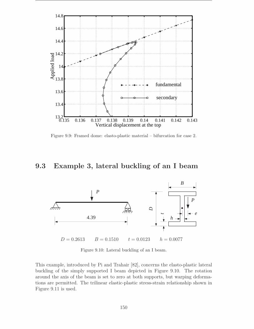
0.135 0.136 0.137 0.138 0.139 0.14 0.141 0.142 0.14313.2

13.4

13.6

13.8

14

14.2

14.4

14.6

14.8

App

lied

load

Vertical displacement at the top

fundamental

secondary

Figure 9.9: Framed dome: elasto-plastic material – bifurcation for case 2.

9.3 Example 3, lateral buckling of an I beam

4.39

P

B

D

t

h

P

e

D = 0.2613 B = 0.1510 t = 0.0123 h = 0.0077

Figure 9.10: Lateral buckling of an I beam.

This example, introduced by Pi and Trahair [82], concerns the elasto-plastic lateralbuckling of the simply supported I beam depicted in Figure 9.10. The rotationaround the axis of the beam is set to zero at both supports, but warping deforma-tions are permitted. The trilinear elastic-plastic stress-strain relationship shown inFigure 9.11 is used.

150

σ

σY

εE

Es

εs

E = 2 · 1011

G = 8 · 1010

σY = 25 · 107

Es = 6 · 109

εs = 0.01375

Figure 9.11: Lateral buckling of an I beam: material parameters.

The results shown in Figure 9.12 were computed with 20 ptw3d elements and 168integration points in the cross-section. Very good agreement with Reference [82]is obtained. It can be noted that, due to the absence of hardening, the perfectstructure (e = 0) presents an unstable bifurcation.

0 0.05 0.1 0.15 0.2 0.25 0.3 0.35 0.460

70

80

90

100

110

120

130

App

lied

load

x 1

000

Central twist rotation

Pi & Trahair

e = 0

e = 0.001

Figure 9.12: Lateral buckling of an I beam: post-buckling behaviour.

151

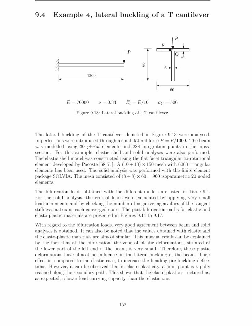
9.4 Example 4, lateral buckling of a T cantilever

1200

P

60

6

6

60

PF

O

E = 70000 ν = 0.33 Et = E/10 σY = 500

Figure 9.13: Lateral buckling of a T cantilever.

The lateral buckling of the T cantilever depicted in Figure 9.13 were analysed.Imperfections were introduced through a small lateral force F = P/1000. The beamwas modelled using 30 ptw3d elements and 288 integration points in the cross-section. For this example, elastic shell and solid analyses were also performed.The elastic shell model was constructed using the flat facet triangular co-rotationalelement developed by Pacoste [68,71]. A (10 + 10)× 150 mesh with 6000 triangularelements has been used. The solid analysis was performed with the finite elementpackage SOLVIA. The mesh consisted of (8 + 8)× 60 = 960 isoparametric 20 nodedelements.

The bifurcation loads obtained with the different models are listed in Table 9.1.For the solid analysis, the critical loads were calculated by applying very smallload increments and by checking the number of negative eigenvalues of the tangentstiffness matrix at each converged state. The post-bifurcation paths for elastic andelasto-plastic materials are presented in Figures 9.14 to 9.17.

With regard to the bifurcation loads, very good agreement between beam and solidanalyses is obtained. It can also be noted that the values obtained with elastic andthe elasto-plastic materials are almost similar. This unusual result can be explainedby the fact that at the bifurcation, the zone of plastic deformations, situated atthe lower part of the left end of the beam, is very small. Therefore, these plasticdeformations have almost no influence on the lateral buckling of the beam. Theireffect is, compared to the elastic case, to increase the bending pre-buckling deflec-tions. However, it can be observed that in elasto-plasticity, a limit point is rapidlyreached along the secondary path. This shows that the elasto-plastic structure has,as expected, a lower load carrying capacity than the elastic one.

152

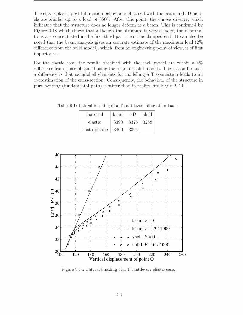
The elasto-plastic post-bifurcation behaviours obtained with the beam and 3D mod-els are similar up to a load of 3500. After this point, the curves diverge, whichindicates that the structure does no longer deform as a beam. This is confirmed byFigure 9.18 which shows that although the structure is very slender, the deforma-tions are concentrated in the first third part, near the clamped end. It can also benoted that the beam analysis gives an accurate estimate of the maximum load (2%difference from the solid model), which, from an engineering point of view, is of firstimportance.

For the elastic case, the results obtained with the shell model are within a 4%difference from those obtained using the beam or solid models. The reason for sucha difference is that using shell elements for modelling a T connection leads to anoverestimation of the cross-section. Consequently, the behaviour of the structure inpure bending (fundamental path) is stiffer than in reality, see Figure 9.14.

Table 9.1: Lateral buckling of a T cantilever: bifurcation loads.

material beam 3D shell

elastic 3390 3375 3258

elasto-plastic 3400 3395

100 120 140 160 180 200 220 240 26030

32

34

36

38

40

42

44

46

Load

P

/ 10

0

Vertical displacement of point O

beam F = P / 1000

solid F = P / 1000

beam F = 0

shell F = 0

Figure 9.14: Lateral buckling of a T cantilever: elastic case.

153

0 10 20 30 40 5030

32

34

36

38

40

42

44

46

Load

P

/ 10

0

Lateral displacement of point O

beam F = P / 1000

solid F = P / 1000

beam F = 0

shell F = 0

Figure 9.15: Lateral buckling of a T cantilever: elastic case.

100 150 200 250 30030

31

32

33

34

35

36

37

38

39

40

Vertical displacement of point O

Load

P

/ 10

0

beam F = P / 1000

solid F = P / 1000

beam F = 0

Figure 9.16: Lateral buckling of a T cantilever: elasto-plastic case.

154

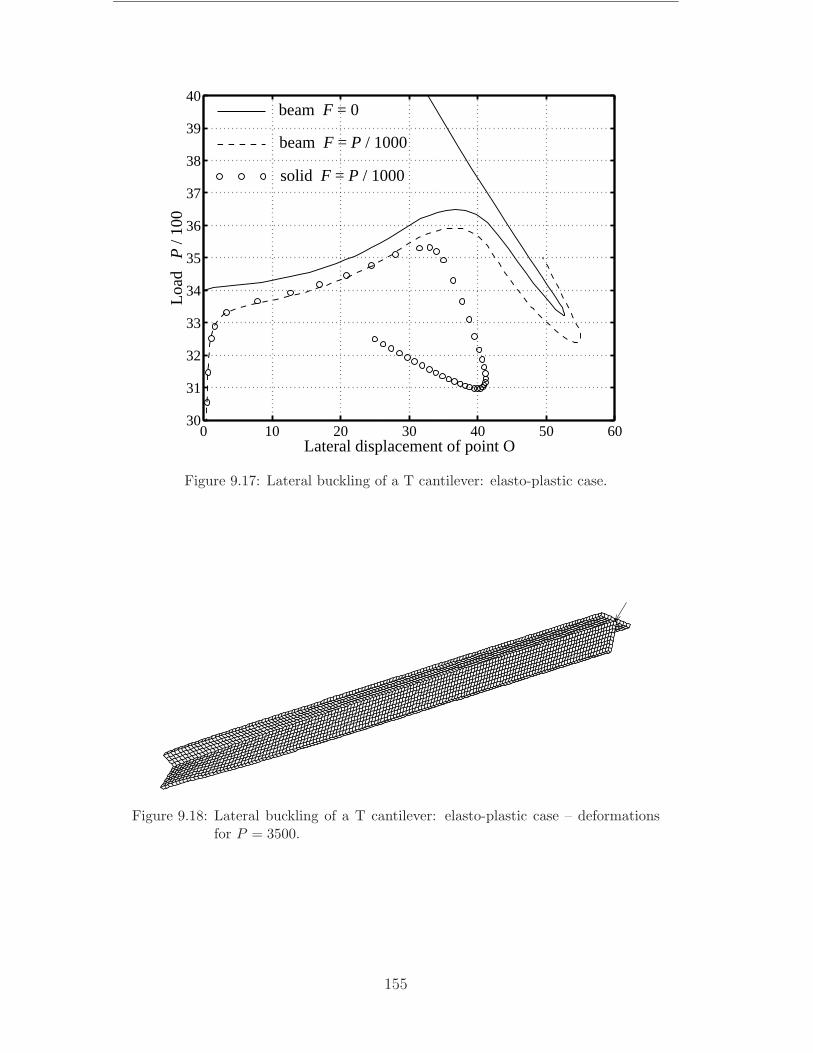
0 10 20 30 40 50 6030

31

32

33

34

35

36

37

38

39

40

Lateral displacement of point O

Load

P

/ 10

0solid F = P / 1000

beam F = P / 1000

beam F = 0

Figure 9.17: Lateral buckling of a T cantilever: elasto-plastic case.

Figure 9.18: Lateral buckling of a T cantilever: elasto-plastic case – deformationsfor P = 3500.

155

9.5 Example 5, buckling by torsion and flexure

x

y

z

60

6

60

F

O

y

z

1800

P

6

O

E = 70000 ν = 0.33 Et = E/5 σY = 20

Figure 9.19: Buckling by torsion and flexure.

The buckling by torsion and flexure of the beam depicted in Figure 9.19 was anal-ysed. All degrees of freedom including warping are set to zero at the left end andonly the axial displacement is permitted at the right end. In order to introduceimperfections, a small lateral force F = P/1000 is applied in the midspan. Thebeam model consists of 40 ptw3d elements and 288 integration points in the cross-section. Elastic shell and solid analyses have also been performed, using the samediscretisations as in the previous example.

The bifurcation loads obtained with the different models are listed in Table 9.2. Itcan be observed that the critical loads obtained using the different models differ byless than 1%.

The load–displacement curves for elastic and elasto-plastic materials are presentedin Figures 9.20 to 9.24. In elasticity, good agreement between the three modelsis obtained until a displacement in the z-direction of about 220. After that, dueto the apparition of local deformations, see Figure 9.22, the shell and solid load–displacement curves present limit points. In the elasto-plastic case, the post-bucklingbehaviour is dominated by the bending mode, and very good agreement betweenbeam and solid models is obtained.

Table 9.2: Buckling by torsion and flexure: bifurcation loads/10000.

material theory [97] beam 3D shell

elastic 8.452 8.444 8.405 8.482

elasto-plastic 1.834 1.845

156

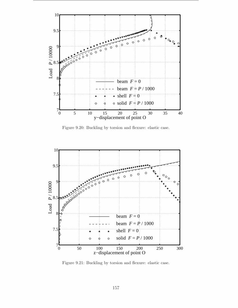
0 5 10 15 20 25 30 35 407

7.5

8

8.5

9

9.5

10

solid F = P / 1000

beam F = P / 1000

beam F = 0

shell F = 0

Load

P

/ 10

000

y−displacement of point O

Figure 9.20: Buckling by torsion and flexure: elastic case.

0 50 100 150 200 250 3007

7.5

8

8.5

9

9.5

10

beam F = P / 1000

solid F = P / 1000

beam F = 0

shell F = 0

Load

P

/ 10

000

z−displacement of point O

Figure 9.21: Buckling by torsion and flexure: elastic case.

157

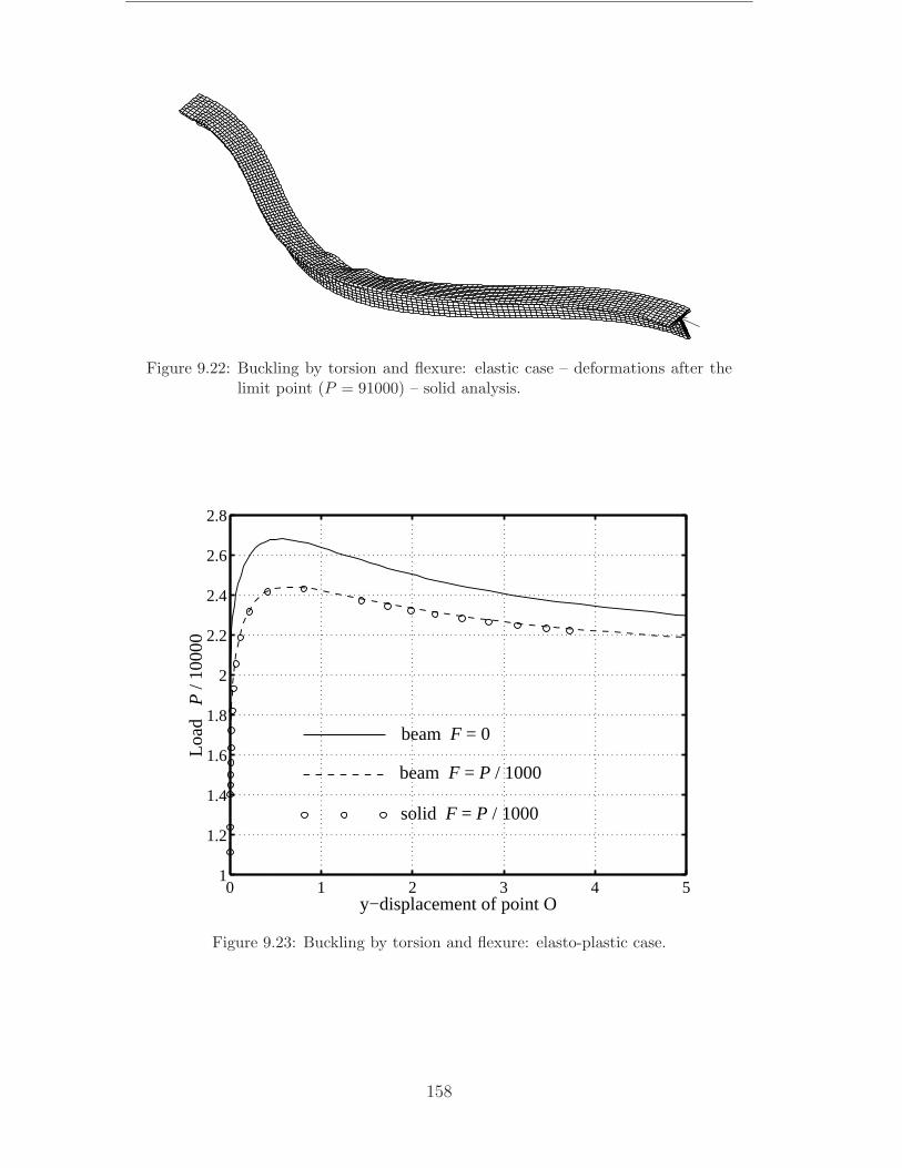
Figure 9.22: Buckling by torsion and flexure: elastic case – deformations after thelimit point (P = 91000) – solid analysis.

0 1 2 3 4 51

1.2

1.4

1.6

1.8

2

2.2

2.4

2.6

2.8

solid F = P / 1000

beam F = P / 1000

beam F = 0

Load

P

/ 10

000

y−displacement of point O

Figure 9.23: Buckling by torsion and flexure: elasto-plastic case.

158

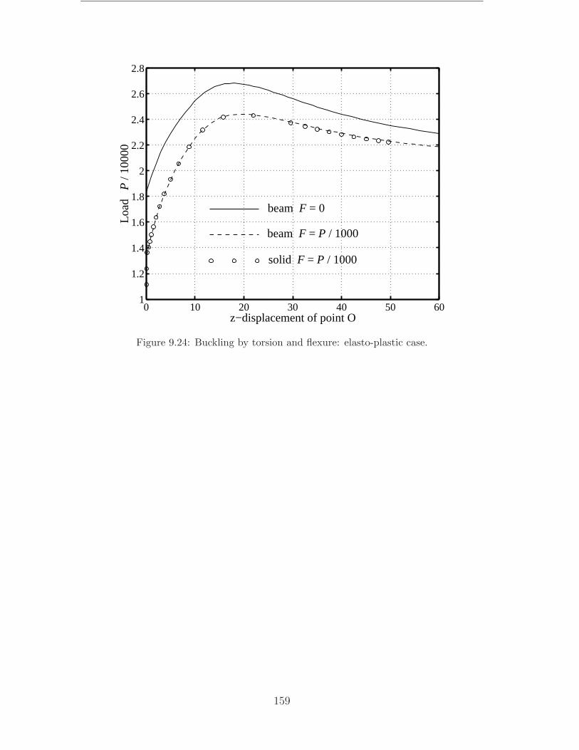
0 10 20 30 40 50 601

1.2

1.4

1.6

1.8

2

2.2

2.4

2.6

2.8

beam F = 0

beam F = P / 1000

solid F = P / 1000

Load

P

/ 10

000

z−displacement of point O

Figure 9.24: Buckling by torsion and flexure: elasto-plastic case.

159

Chapter 10

Conclusions and future research

In this last chapter, conclusions about the numerical computations performed inChapters 6 to 9 and suggested directions for future research are presented.

10.1 Conclusions

The purpose of this thesis was to implement efficient co-rotational beam elementsand branch-switching procedures in order to study elastic and elasto-plastic insta-bility problems. These elements and procedures, presented in details in Chapters 3to 5 have been tested through a large numbers of examples in Chapters 6 to 9. Fromthe analysis of these numerical applications, several conclusions can be stated.

2D beam element formulation

The co-rotational approach for 2D beam elements is a well known topic and theobjective of the present work was to compare three local elasto-plastic elements.

Both Timoshenko and Bernoulli elements gave close numerical results for framesconsisting of slender beams. This observation was expected since in such cases theshear deformations can be neglected. It is therefore recommended to use Bernoullielements for these structures since the resolution of the constitutive equations ateach Gauss point does not require any implicit process.

Only small variations have been observed between load–displacement diagrams com-puted with seven and fifteen integration points along the beam depth. From anengineering point of view, these differences are negligible and a small number ofGauss points should be used for the analysis of large structures.

Concerning Bernoulli elements, the shallow arch approach should be preferred tothe linear one since identical numerical results can be obtained with fewer elements.This point, already observed in [73] for elastic structures, was not evident in elasto-plasticity: by decreasing the number of elements, the number of sections in thestructure where Gauss integrations are performed is also reduced, and consequently,

161

zones of plastification or elastic unloading are modelled with lower accuracy. How-ever, this does not seem to have any significant effect on load–displacement diagrams.

3D beam element formulation

Compared to Pacoste and Eriksson [73], the 3D co-rotational formulation developedin Chapter 4 presents new items concerning the parameterisation of the rotations,the definition of the local frame, the inclusion of warping effects through the intro-duction of a seventh nodal degree of freedom and the consideration of rigid links. Allthese improvements have been tested in a large number of examples in Chapters 7and 9. The present results have been compared with results found in the literatureand also with analyses performed using shell and solid elements. It can then beconcluded that the elements developed in this thesis can be used to study any largedisplacements and rotations problems involving non-linear coupling between axial,bending and torsional-warping effects. In addition, any cross-section shape can beconsidered. In fact, concerning the element formulation, the only restriction residesin the small strain assumption.

One of the main properties of the co-rotational formulation adopted in this thesis, isits independence of the local strains assumptions used to derive local internal forcevectors and tangent stiffness matrices. Using this property most authors use linearstrains at the level of the local element definition. However, as shown by severalof the numerical examples included in Chapter 7, this type of elements may giveincorrect results for problems where torsional effects are important.

For these reasons, the displacement field proposed by Gruttmann et al. [41] hasbeen adopted and used to construct a consistent second order approximation tothe Green-Lagrange strains, at the level of the local element frame. The resultingexpressions have been further simplified by neglecting the non-linear terms in theexpression of shear strains ε12 and ε13 and in the bending curvatures. In fact itappears that the only important non-linear term is the Wagner term, i.e. 1

2r2ϑ2

1,1,in the expression of ε11. Some authors (see e.g. [55]) replace this term by its averagevalue over the cross-section. The tests performed by the author have shown thatthis simplification is not acceptable.

Another characteristic of the co-rotational approach is that the material non-linearityis only present at the level of the local deformations and does not affect the co-rotational framework. Hence, due to the simplicity of the local strains expression,the derivation of elasto-plastic local elements is rather easy. Using linear interpo-lations, Timoshenko elements have been developed. Based on the work done inSection 4.3.1, Bernoulli elements can also be derived without difficulties.

Branch-switching in elasto-plasticity

Two methods of branch-switching in elasto-plasticity have been presented in Section5.3. In the first one, the bifurcation point is isolated by successive bisections andthe branch-switching is operated by using the eigenvector associated to the negative

162

eigenvalue. In the second one, introduced by Petryk [76–81], an energy approach isused to select automatically the stable post-bifurcation path.

In most studied examples in Chapters 6 and 9, both methods work very well andconvergence to the first point of the secondary path is obtained after 4–7 iterations.However, if the bifurcation is unstable (examples 6.3 and 9.3) or if the stable partof the secondary path is very small (example 9.2), the minimisation procedure cannot be employed. On the other hand, if an arc-length procedure is used, the modeinjection method does not ensure convergence to the secondary path, in particular forstructures exhibiting a tangent bifurcation (examples 6.5 and 9.2). The conclusion ofthe author is that the best alternative is to use the mode injection method togetherwith a displacement control procedure and to take as control a displacement or arotation which is zero along the fundamental path.

Direct computation of elastic critical points

In Section 5.2, a new procedure for the direct computation of elastic critical pointshas been presented. Compared to the approach of Wriggers et al. [104, 105], twonew ideas have been introduced. First, the condition of criticality is expressedby a scalar equation. Next, the present method combines iterations based on theextended system obtained by the equilibrium equations and the criticality conditionwith iterations based only on the equilibrium equations under load or displacementcontrol.

The performances of the present method and the classical approach [104, 105] havebeen compared through eight numerical examples in Chapter 8. In most of thecases, both approaches give similar results. However, if the non-linearity betweenthe initial point and the critical one is important, as in examples 8.1, 8.6 and 8.7, theconvergence properties of the present method are better. It can then be concludedthat the numerical procedure presented in this thesis is an interesting alternativefor the direct computation of critical points.

10.2 Future research

The work done in this thesis can be extended in three directions which are nowbriefly presented.

Element formulation

The co-rotational formulation presented in this thesis is based on a spatial repre-sentation of the rotations, see Section 4.1. Another possibility is to derive elementsusing a material representation. As pointed out by Ibrahimbegovic [51], a materialapproach is more suitable in the context of dynamics and time-stepping schemes.

163

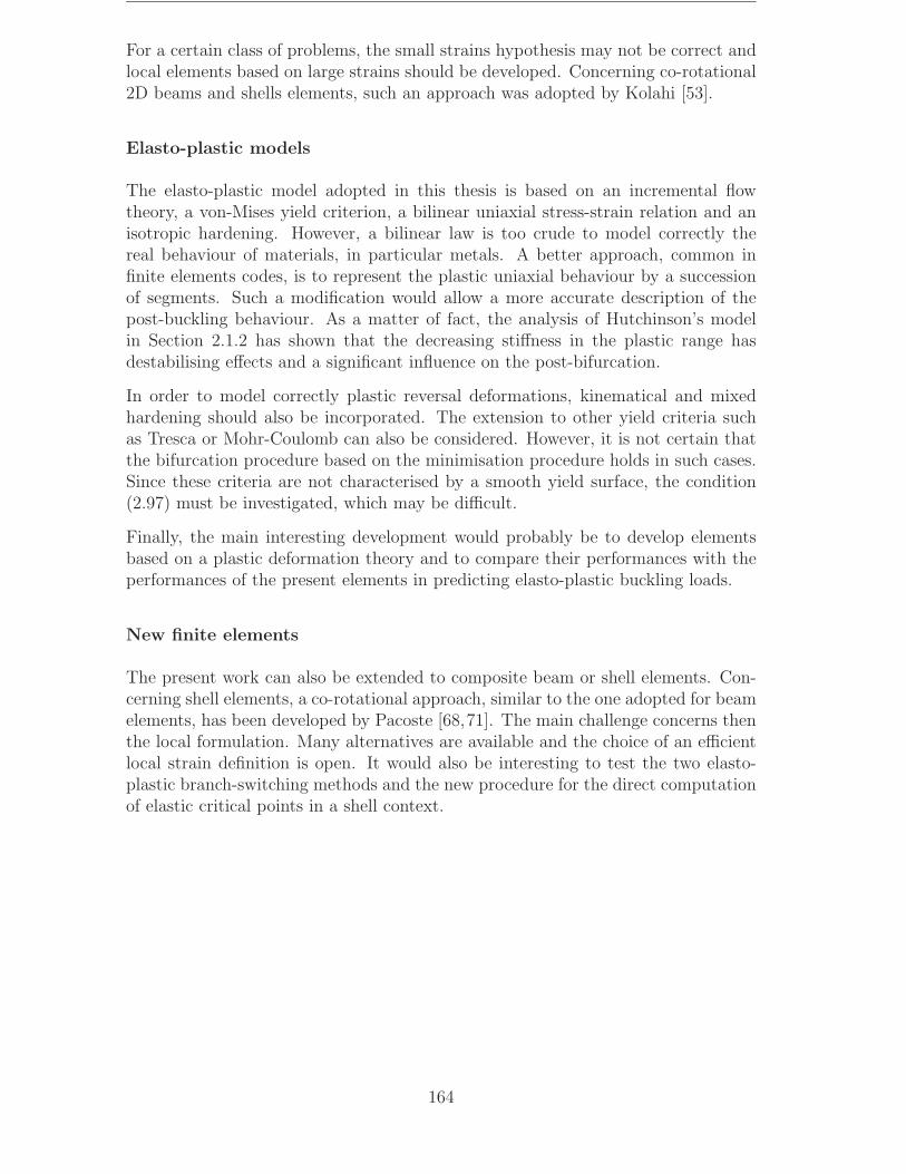
For a certain class of problems, the small strains hypothesis may not be correct andlocal elements based on large strains should be developed. Concerning co-rotational2D beams and shells elements, such an approach was adopted by Kolahi [53].

Elasto-plastic models

The elasto-plastic model adopted in this thesis is based on an incremental flowtheory, a von-Mises yield criterion, a bilinear uniaxial stress-strain relation and anisotropic hardening. However, a bilinear law is too crude to model correctly thereal behaviour of materials, in particular metals. A better approach, common infinite elements codes, is to represent the plastic uniaxial behaviour by a successionof segments. Such a modification would allow a more accurate description of thepost-buckling behaviour. As a matter of fact, the analysis of Hutchinson’s modelin Section 2.1.2 has shown that the decreasing stiffness in the plastic range hasdestabilising effects and a significant influence on the post-bifurcation.

In order to model correctly plastic reversal deformations, kinematical and mixedhardening should also be incorporated. The extension to other yield criteria suchas Tresca or Mohr-Coulomb can also be considered. However, it is not certain thatthe bifurcation procedure based on the minimisation procedure holds in such cases.Since these criteria are not characterised by a smooth yield surface, the condition(2.97) must be investigated, which may be difficult.

Finally, the main interesting development would probably be to develop elementsbased on a plastic deformation theory and to compare their performances with theperformances of the present elements in predicting elasto-plastic buckling loads.

New finite elements

The present work can also be extended to composite beam or shell elements. Con-cerning shell elements, a co-rotational approach, similar to the one adopted for beamelements, has been developed by Pacoste [68,71]. The main challenge concerns thenthe local formulation. Many alternatives are available and the choice of an efficientlocal strain definition is open. It would also be interesting to test the two elasto-plastic branch-switching methods and the new procedure for the direct computationof elastic critical points in a shell context.

164

Bibliography

[1] J.H. Argyris, B. Boni, U. Hindenlang, and M. Kleiber. Finite element analysisof two- and three-dimensional elasto-plastic frames—the natural approach.Comput. Methods Appl. Mech. Engrg., 35:221–248, 1982.

[2] S. Baba and T. Kajita. Plastic analysis of torsion of a prismatic beam. Int.J. Numer. Meth. Engng., 18:927–944, 1982.

[3] J.L. Batoz and G. Dhatt. Modelisation Des Structures Par Elements Finis,Volume 1: Solides Elastiques. Hermes, Paris, 1990. In French.

[4] J.L. Batoz and G. Dhatt. Modelisation Des Structures Par Elements Finis,Volume 2: Poutres et Plaques. Hermes, Paris, 1990. In French.

[5] J.-M. Battini. Plastic Instability Analysis of Plane Frames Using a Co-Rotational Approach. Licentiate Thesis, Department of Structural Engineer-ing, KTH, Stockholm, 1999.

[6] J.-M. Battini and C. Pacoste. Co-rotational beam elements with warpingeffects in instability problems. Accepted by Comput. Methods Appl. Mech.Engrg.

[7] J.-M. Battini and C. Pacoste. Elements poutres co-rotationels avec gauchisse-ment. Proceedings CSMA 5eme colloque national en calcul des structures,Giens 2001. In French.

[8] J.-M. Battini and C. Pacoste. Minimal augmentation procedure for the directcomputation of critical points. Submitted to Comput. Methods Appl. Mech.Engrg.

[9] J.-M. Battini and C. Pacoste. Plastic instability of beam structures usingco-rotational elements. Submitted to Comput. Methods Appl. Mech. Engrg.

[10] Z.J. Bazant. Stability of Structures. Oxford University Press, 1991.

[11] B. Budianski. A reassessment of deformation theories of plasticity. J. Appl.Mech., 26:259–264, 1959.

[12] A. Cardona and A. Huespe. Evaluation of simple bifurcation points and post-critical path in large finite rotation problems. Comput. Methods Appl. Mech.Engrg., 175:137–156, 1999.

165

[13] C.N. Chen. Study on the reliability of Shanley’s plastic buckling model byusing the finite element method. Proceedings of the 1994 Pressure Vessels andPiping Conference, 277:127–134, 1994.

[14] N.C. Chen. A finite element study on Shanley’s plastic buckling theory ofshort columns. Computers and Structures, 59(5):975–982, 1996.

[15] Y. Cheng, H. Fang, and W. Lu. Imperfection sensitivity analysis of a rect-angular column compressed into the plastic range. Applied Mathematics andMechanics, 19(1):9–14, 1998.

[16] Y. Cheng, W. Lu, and H. Fang. Plastic post-buckling of a simply supportedcolumn with a rectangular cross-section. Applied Mathematics and Mechanics,16(8):713–722, 1995.

[17] C. Cichon. Large displacements in-plane analysis of elastic-plastic frames.Computers and Structures, 19:737–745, 1984.

[18] A. Cimetiere, A. Elkoulani, and A. Leger. Buckling and post-buckling ofan elastic-plastic simple model. Comptes rendus de l’academie des sciences,Paris, 319:1263–1269, 1994.

[19] A. Cimetiere and A. Leger. Some problems about elastic-plastic post-buckling.Int. J. Solids Structures, 33(10):1519–1533, 1996.

[20] A. Considere. Resistance des pieces comprimees. In Paris Librairie Polytech-nique, editor, Congres International Des Procedes de Construction, 1891. InFrench.

[21] R.D. Cook, D.S. Malkus, and M.E. Plesha. Concepts and Applications ofFinite Element Analysis. Wiley, Chichester, third edition, 1989.

[22] M.A. Crisfield. A consistent co-rotational formulation for non-linear, three-dimensional, beam-elements. Comput. Methods Appl. Mech. Engrg., 81:131–150, 1990.

[23] M.A. Crisfield. Non-Linear Finite Element Analysis of Solids and Structures,Volume 1: Essentials. Wiley, Chichester, 1991.

[24] M.A. Crisfield. Non-Linear Finite Element Analysis of Solids and Structures,Volume 2: Advanced Topics. Wiley, Chichester, 1997.

[25] M.A. Crisfield and D. Tan. A low-order large-strain quadrilateral shell element.In European Congress on Computational Methods in Applied Sciences andEngineering, Barcelona, 11-14 September 2000. ECCOMAS 2000.

[26] R. de Borst. Computation of post-bifurcation and post-failure behavior ofstrain-softening solids. Computers and Structures, 25(2):211–224, 1987.

[27] V. de Ville de Goyet. L’analyse Statique Non Lineaire Par la Methode DesElements Finis Des Structures Spatiales Formees de Poutres a Section NonSymetrique. PhD thesis, Universite de Liege, 1988-1989.

166

[28] R.H. Dodds. Numerical techniques for plasticity computations in finite elementanalysis. Computers and Structures, 26:767–779, 1987.

[29] M.S. El Naschie. Stress, Stability and Chaos in Structural Engineering: AnEnergy Approach. McGraw-Hill, 1990.

[30] A. Eriksson. Fold lines sensitivity analyses in structural instability. Comput.Methods Appl. Mech. Engrg., 114:77–101, 1994.

[31] A. Eriksson. Equilibrium subsets for multi-parametric structural analysis.Comput. Methods Appl. Mech. Engrg., 140:305–327, 1997.

[32] A. Eriksson. Structural instability analyses based on generalised path-following. Comput. Methods Appl. Mech. Engrg., 156:45–74, 1998.

[33] A. Eriksson and C. Pacoste. Solution surfaces and generalised paths in non-linear structural mechanics. Int. J. Struct. Stability and Dynamic, 1(1), 2001.

[34] A. Eriksson, C. Pacoste, and A. Zdunek. Numerical analysis of complex in-stability behaviour using incremental-iterative strategies. Comput. MethodsAppl. Mech. Engrg., 179:265–305, 1999.

[35] C.A. Felippa. A systematic approach to the element-independent corotationaldynamics of finite elements. In Int. Conf. Computational Methods for Shelland Spatial Structures, Papadrakakis, M., Samartin, A. and Onate, E. (Eds.)ISASR-NTUA, Athens, Greece 2000. IASS-IACM 2000.

[36] R. Fletcher. Practical Methods of Optimization. Wiley, second edition, 1987.

[37] K. Forsell. Instability Analyses of Structures under Dynamic Loads. PhDthesis, Department of Structural Engineering, KTH, Stockholm, 2000.

[38] Y. Goto, T. Yoshimitsu, and M. Obata. Elliptic integral solutions of planeelastica with axial and shear deformations. Int. J. Solids Structures, 26(4):375–390, 1990.

[39] F. Gruttmann, R. Sauer, and W. Wagner. Shear stresses in prismatic beamswith arbitrary cross-sections. Int. J. Numer. Meth. Engng., 45:865–889, 1999.

[40] R. Gruttmann, R. Sauer, and W. Wagner. A geometrical nonlinear eccentric3d-beam element with arbitrary cross-section. Comput. Methods Appl. Mech.Engrg., 160:383–400, 1998.

[41] R. Gruttmann, R. Sauer, and W. Wagner. Theory and numerics of three-dimensional beams with elastoplastic behaviour. Int. J. Num. Meth. Engng.,48:1675–1702, 2000.

[42] W. Guggenberger. Nonlinear analysis of space frame structures–large rotationformulations and their consistent approximations for moderate rotations. InEuropean Congress on Computational Methods in Applied Sciences and Engi-neering, Barcelona, 11-14 September 2000. ECCOMAS 2000.

167

[43] B. Haugen and C.A. Felippa. A unified formulation of co-rotational finiteelements: I. theory. Technical Report CU-CAS-95-06, Center for AerospaceStructures, Dept of Aerospace Engineering, U. Colorado, Boulder.

[44] B. Haugen and C.A. Felippa. A unified formulation of co-rotational fi-nite elements: II. applications. Technical Report CU-CAS-95-06, Center forAerospace Structures, Dept of Aerospace Engineering, U. Colorado, Boulder.

[45] R. Hill. A general theory of uniqueness and stability in elastic-plastic solids.J. Mech. Phys. Solids, 6:236–249, 1958.

[46] R. Hill and M. J. Sewell. A general theory of inelastic column failure. J. Mech.Phys. Solids, 8:105–111, 1960.

[47] K.M. Hsiao and W.Y. Lin. A co-rotational finite element formulation forbuckling and postbuckling analyses of spatial beams. Comput. Methods Appl.Mech. Engrg., 188:567–594, 2000.

[48] J.W. Hutchinson. Imperfection sensitivity in the plastic range. J. Mech. Phys.Solids, 21:191–204, 1973.

[49] J.W. Hutchinson. Post-bifurcation behaviour in the plastic range. J. Mech.Phys. Solids, 21:163–190, 1973.

[50] J.W. Hutchinson. Plastic buckling. Advances in Appl. Mech., 14:67–144, 1974.

[51] A. Ibrahimbegovic. On the choice of finite rotation parameters. Comput.Methods Appl. Mech. Engrg., 149:49–71, 1997.

[52] A. Ibrahimbegovic and M. Al Mikad. Quadratically convergent direct calcu-lation of critical points for 3d structures undergoing finite rotations. Comput.Methods. Appl. Mech. Engrg., 189:107–120, 2000.

[53] A.S. Kolahi. Co-Rotational Methods for Small and Large Strain Beams, Sheetsand Shells. PhD thesis, Dept. of Aeronautics, Imperial College, London, 1998.

[54] K. Kondoh and N. Atluri. Large-deformation, elasto-plastic analysis of framesunder nonconservative loading, using explicitly derived tangent stiffness basedon assumed stresses. Comp. Mech., 2:1–25, 1987.

[55] R. Kouhia. On kinematical relations of spatial framed structures. Computersand Structures, 40(5):1185–1191, 1991.

[56] R. Kouhia and M. Tuomala. Static and dynamic analysis of space frames usingsimple Timoshenko type elements. Int. J. Num. Meth. Engng., 36:1189–1221,1993.

[57] S.H. Lee. Rudimentary considerations for effective line search method in non-linear finite element analysis. Computers and Structures, 32(6):1287–1301,1989.

168

[58] A. Leger and M. Potier-Ferry. Sur le flambage plastique. J. Mecanique Theor.Appl., 7:819–857, 1988. In French.

[59] T. Lidstrom. Computational Methods for Finite Element Instability Analyses.PhD thesis, Department of Structural Engineering, KTH, Stockholm, 1996.

[60] K. Moon-Young, C. Sung-Pil, and K. Sung-Bo. Spatial stability analysis ofthin-walled space frames. Int. J. Num. Meth. Engng., 39:499–525, 1996.

[61] A. Needleman and V. Tvergaard. An analysis of the imperfection sensitivityof square elastic-plastic plates under compression. Int. J. Solids Structures,12:185–201, 1976.

[62] Q.S. Nguyen. Bifurcation and postbifurcation analysis in plasticity and brittlefracture. J. Mech. Phys. Solids, 33:303–324, 1987.

[63] Q.S. Nguyen. Bifurcation and stability of time-independent standard dissipa-tive systems. In Q.S. Nguyen, editor, CISM Courses and Lectures No. 327 :Bifurcation and Stability of Dissipative Systems. Springer-Verlag, 1993.

[64] B. Nour-Omid and C.C. Rankin. Finite rotation analysis and consistent lin-earization using projectors. Comput. Methods Appl. Mech. Engrg., 93:353–384,1991.

[65] A. Olsson. Object-Oriented Finite Element Algorithms. Licenciate Thesis,Department of Structural Engineering, KTH, Stockholm, 1997.

[66] M. Ortiz and E. P. Popov. Accuracy and stability of integration algorithms forelastoplastic constitutive relations. Int. J. Num. Meth. Engng., 21:1561–1576,1985.

[67] D.R.J. Owen and E. Hinton. Finite Elements in Plasticity: Theory and Prac-tice. Pineridge Press Limited, Swansea UK, 1980.

[68] C. Pacoste. Co-rotational flat facet triangular elements for shell instabilityanalysis. Comput. Methods Appl. Mech. Engrg., 156:75–110, 1998.

[69] C. Pacoste and J.-M. Battini. Calcul des chemins d’equilibres post-critiques.Proceedings CSMA 5eme colloque national en calcul des structures, Giens2001. In French.

[70] C. Pacoste, J.-M. Battini, and A. Eriksson. Parameterisation of rotations inco-rotational elements. Proceedings Euromech 2000, Metz.

[71] C. Pacoste and A. Eriksson. Element formulation and numerical techniquesfor stability problems in shells. Accepted by Comput. Methods Appl. Mech.Engrg.

[72] C. Pacoste and A. Eriksson. Element behaviour in post-critical plane frameanalysis. Comput. Methods Appl. Mech. Engrg., 125:319–343, 1995.

169

[73] C. Pacoste and A. Eriksson. Beam elements in instability problems. Comput.Methods Appl. Mech. Engrg., 144:163–197, 1997.

[74] M.S. Park and B.C. Lee. Geometrically non-linear and elastoplastic three-dimensional shear flexible beam element of von-Mises-type hardening material.Int. J. Num. Meth. Engng., 39:383–408, 1996.

[75] U. Perego. Explicit backward difference operators and consistent predictors forlinear hardening elastic-plastic constitutive laws. SM Archives, 13(2):65–102,1988.

[76] H. Petryk. The energy criteria of instability in time-independent inelasticsolids. Arch. Mech., 43:519–545, 1991.

[77] H. Petryk. Theory of bifurcation and instability in time-independent plasticity.In Q.S. Nguyen, editor, CISM Courses and Lectures No. 327—Bifurcation andStability of Dissipative Systems, pages 95–152. Springer-Verlag, 1993.

[78] H. Petryk. Instability of plastic deformation processes. In T. Tatsumi et Al.,editor, Theoretical and Applied Mechanics, Proc.XIXth IUATAM Congress,Kyoto, pages 497–516. Elsevier, Amsterdam, 1997.

[79] H. Petryk and K. Thermann. Second-order bifurcation in elastic-plastic solids.J. Mech. Phys. Solids, 33(6):577–593, 1985.

[80] H. Petryk and K. Thermann. On discretized plasticity problems with bifurca-tions. Int. J. Solids Structures, 29(6):745–765, 1992.

[81] H. Petryk and K. Thermann. On post-bifurcation paths in plastic deforma-tion process. In D.R.J. Owen, editor, Computational Plasticity. Fundamentalsand Applications—Part I. Proceedings of the Third Int. Conf., pages 593–604.Pineridge Press, 1992.

[82] Y.L. Pi and N.S. Trahair. Nonlinear inelastic analysis of steel beam-columns:II: Applications. Journal of Structural Engineering, 120(7):2062–2085, 1994.

[83] C.C. Rankin and F.A. Brogan. An element-independent co-rotational proce-dure for the treatment of large rotations. ASME J. Pressure Vessel Tchn.,108:165–174, 1986.

[84] C.C. Rankin and B. Nour-Omid. The use of projectors to improve finiteelement performance. Computers and Structures, 30:257–267, 1988.

[85] M. Ristinmaa and J. Tryding. Exact integration of constitutive equations inelasto-plasticity. Int. J. Num. Meth. Engng., 36:2525–2544, 1993.

[86] R. Sauer. Eine Einheitliche Finite-Element-Formulierung Fur Stab- und Scha-lentragwerke mit Endlichen Rotationen. PhD thesis, Bericht Nr. 4, Institutfur Baustatik, Universitat Karlsruhe, 1998. In German.

[87] M.J. Sewell. A Survey of Plastic Buckling. Solid Mechanics Division, Univer-sity of Waterloo, Waterloo, Ontario, Canada, 1972.

170

[88] F.R. Shanley. Inelastic column theory. J. Aero. Science, 14:261–267, 1947.

[89] J.C. Simo, J.G. Kennedy, and S. Govindjee. Non-smooth multisurface plas-ticity and viscoplasticity. Loading/unloading conditions and numerical algo-rithms. Int. J. Num. Meth. Engng., 26:2161–2185, 1988.

[90] J.C. Simo and R.L. Taylor. Consistent tangent operators for rate-independentelastoplasticity. Comput. Methods Appl. Mech. Engrg., 48:101–118, 1985.

[91] J.C. Simo and R.L. Taylor. A return mapping algorithm for plane stresselastoplasticity. Int. J. Num. Meth. Engng., 22:649–670, 1986.

[92] J.C. Simo and L. Vu-Quoc. A three-dimensional finite-strain rod model. partII: Computational aspects. Comput. Methods Appl. Mech. Engrg., 58:79–116,1986.

[93] J.C. Simo and L. Vu-Quoc. A geometrically-exact rod model incorporatingshear and torsion-warping deformation. Int. J. Solids Structures, 27(3):371–393, 1991.

[94] X.M. Su and W. Lu. Postbuckling and imperfection sensitivity analysis ofstructures in the plastic range—part 1: Model analysis. Thin-Walled Struc-tures, 10:263–275, 1990.

[95] J.G. Teigen. Nonlinear Analysis of Concrete Structures Based on a 3D Shear-Beam Element Formulation. PhD thesis, Department of Mathematics, Me-chanics Division, University of Oslo, Norway, 1994.

[96] J.M.T. Thompson and G.W. Hunt. Elastic Instability Phenomena. Wiley,Chichester, 1984.

[97] S.P. Timoshenko and J.M. Gere. Theory of Elastic Stability. Second Edition,McGraw-Hill, Tokyo, 1961.

[98] N. Triantafyllidis. On the bifurcation and postbifurcation analysis of elastic-plastic solids under general prebifurcation conditions. J. Mech. Phys. Solids,31(6):499–510, 1983.

[99] A.M.A. van der Heijden. A study of Hutchinson’s plastic buckling model. J.Mech. Phys. Solids, 27:441–464, 1979.

[100] H. van der Veen. The Significance and Use of Eigenvalues and Eigenvectorsin the Numerical Analysis of Elasto-Plastic Soils. PhD thesis, Faculty of CivilEngineering and Geosciences, Delft University of Technology, Netherlands,1998.

[101] H. van der Veen, K. Vuik, and R. de Borst. Branch switching techniquesfor bifurcation in soil deformation. Comput. Methods Appl. Mech. Engrg.,190:707–719, 2000.

[102] T. von Karman. Untersuchungen uber Knickfestigkeit. In Verein DeutscherIngenieure, editor, Mitteilungen uber Forschungsarbeiten, 1910. In German.

171

[103] W. Wagner and F. Gruttmann. Finite element analysis of Saint-Venant torsionproblem with exact integration of the elastic-plastic constitutive equations.Comput. Methods Appl. Mech. Engrg., 190:3831–3848, 2001.

[104] P. Wriggers and J.C. Simo. A general procedure for the direct computation ofturning and bifurcation points. Int. J. Num. Meth. Engrg., 30:155–176, 1990.

[105] P. Wriggers, W. Wagner, and C. Miehe. A quadratically convergent proce-dure for the calculation of stability points in finite element analysis. Comput.Methods Appl. Mech. Engrg., 70:329–347, 1988.

172

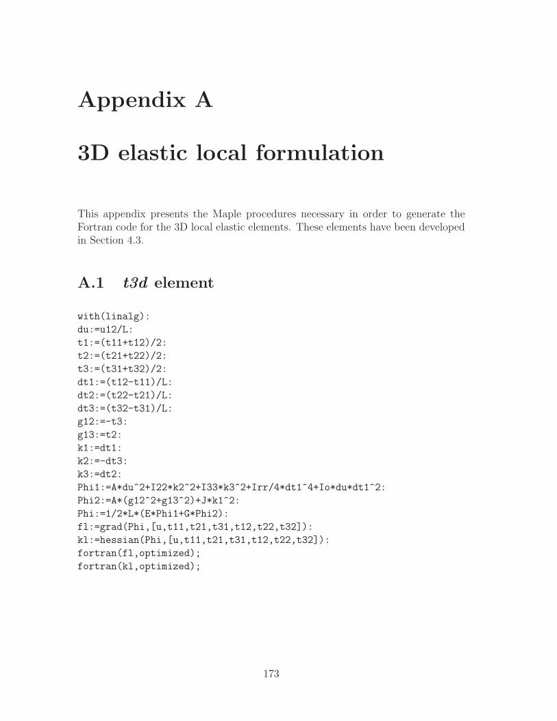
Appendix A

3D elastic local formulation

This appendix presents the Maple procedures necessary in order to generate theFortran code for the 3D local elastic elements. These elements have been developedin Section 4.3.

A.1 t3d element

with(linalg):

du:=u12/L:

t1:=(t11+t12)/2:

t2:=(t21+t22)/2:

t3:=(t31+t32)/2:

dt1:=(t12-t11)/L:

dt2:=(t22-t21)/L:

dt3:=(t32-t31)/L:

g12:=-t3:

g13:=t2:

k1:=dt1:

k2:=-dt3:

k3:=dt2:

Phi1:=A*du^2+I22*k2^2+I33*k3^2+Irr/4*dt1^4+Io*du*dt1^2:

Phi2:=A*(g12^2+g13^2)+J*k1^2:

Phi:=1/2*L*(E*Phi1+G*Phi2):

fl:=grad(Phi,[u,t11,t21,t31,t12,t22,t32]):

kl:=hessian(Phi,[u,t11,t21,t31,t12,t22,t32]):

fortran(fl,optimized);

fortran(kl,optimized);

173

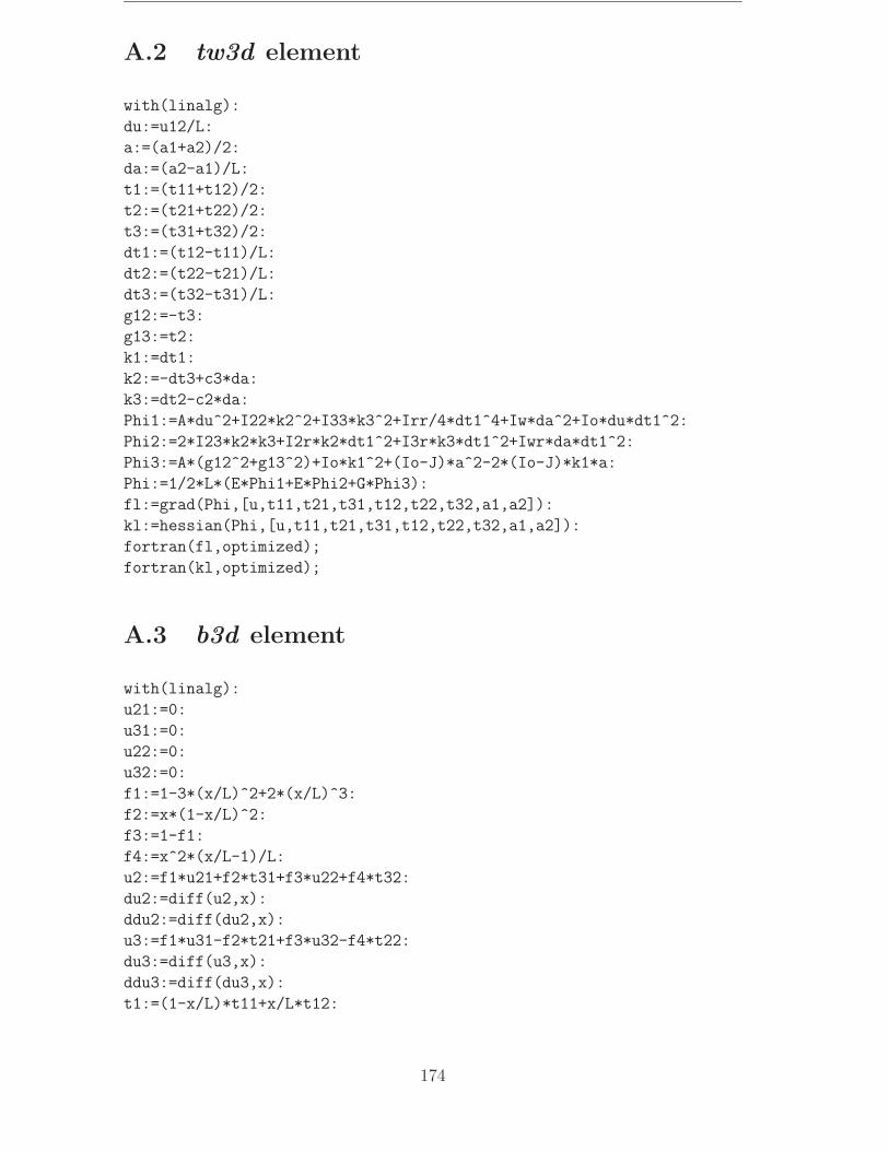
A.2 tw3d element

with(linalg):

du:=u12/L:

a:=(a1+a2)/2:

da:=(a2-a1)/L:

t1:=(t11+t12)/2:

t2:=(t21+t22)/2:

t3:=(t31+t32)/2:

dt1:=(t12-t11)/L:

dt2:=(t22-t21)/L:

dt3:=(t32-t31)/L:

g12:=-t3:

g13:=t2:

k1:=dt1:

k2:=-dt3+c3*da:

k3:=dt2-c2*da:

Phi1:=A*du^2+I22*k2^2+I33*k3^2+Irr/4*dt1^4+Iw*da^2+Io*du*dt1^2:

Phi2:=2*I23*k2*k3+I2r*k2*dt1^2+I3r*k3*dt1^2+Iwr*da*dt1^2:

Phi3:=A*(g12^2+g13^2)+Io*k1^2+(Io-J)*a^2-2*(Io-J)*k1*a:

Phi:=1/2*L*(E*Phi1+E*Phi2+G*Phi3):

fl:=grad(Phi,[u,t11,t21,t31,t12,t22,t32,a1,a2]):

kl:=hessian(Phi,[u,t11,t21,t31,t12,t22,t32,a1,a2]):

fortran(fl,optimized);

fortran(kl,optimized);

A.3 b3d element

with(linalg):

u21:=0:

u31:=0:

u22:=0:

u32:=0:

f1:=1-3*(x/L)^2+2*(x/L)^3:

f2:=x*(1-x/L)^2:

f3:=1-f1:

f4:=x^2*(x/L-1)/L:

u2:=f1*u21+f2*t31+f3*u22+f4*t32:

du2:=diff(u2,x):

ddu2:=diff(du2,x):

u3:=f1*u31-f2*t21+f3*u32-f4*t22:

du3:=diff(u3,x):

ddu3:=diff(du3,x):

t1:=(1-x/L)*t11+x/L*t12:

174

dt1:=diff(t1,x):

k1:=dt1:

k2:=-ddu2:

k3:=-ddu3:

eav:=u12/L+1/2/L*int(du2^2+du3^2+Io/A*dt1^2,x=0..L):

Phi1:=A*eav^2+I22*k2^2+I33*k3^2+1/4*(Irr-Io^2/A)*dt1^4:

Phi:=1/2*int(E*Phi1+G*J*k1^2,x=0..L):

fl:=grad(Phi,[u,t11,t21,t31,t12,t22,t32]):

kl:=hessian(Phi,[u,t11,t21,t31,t12,t22,t32]):

fortran(fl,optimized);

fortran(kl,optimized);

A.4 bw3d element

with(linalg):

u21:=0:

u31:=0:

u22:=0:

u32:=0:

f1:=1-3*(x/L)^2+2*(x/L)^3:

f2:=x*(1-x/L)^2:

f3:=1-f1:

f4:=x^2*(x/L-1)/L:

u2:=f1*u21+f2*t31+f3*u22+f4*t32:

du2:=diff(u2,x):

ddu2:=diff(du2,x):

u3:=f1*u31-f2*t21+f3*u32-f4*t22:

du3:=diff(u3,x):

ddu3:=diff(du3,x):

t1:=f1*t11+f2*a1+f3*t12+f4*a2:

dt1:=diff(t1,x):

ddt1:=diff(dt1,x):

k1:=dt1:

k2:=-ddu2+c3*ddt1:

k3:=-ddu3-c2*ddt1:

eav:=u12/L+1/2/L*int(du2^2+du3^2+Io/A*dt1^2,x=0..L):

Phi1:=A*eav^2+I22*k2^2+I33*k3^2+1/4*(Irr-Io^2/A)*dt1^4+Iw*ddt1^2:

Phi2:=2*I23*k2*k3+I2r*k2*dt1^2+I3r*k3*dt1^2+Iwr*ddt1*dt1^2:

Phi3:=G*J*k1^2:

Phi:=1/2*int(E*Phi1+E*Phi2+G*Phi3,x=0..L):

fl:=grad(Phi,[u,t11,t21,t31,t12,t22,t32,a1,a2]):

kl:=hessian(Phi,[u,t11,t21,t31,t12,t22,t32,a1,a2]):

fortran(fl,optimized);

fortran(kl,optimized);

175

Appendix B

Warping function

The purpose of this appendix is to describe the theoretical and numerical aspectsrelated to the computation of the warping function ω and cross-section quantitiesintroduced in equation (4.130). The theoretical aspects are taken from Batoz andDhatt [3] and Gruttmann et al. [39]. Concerning the finite element implementation,the description of isoparametric quadratic plane elements can be found e.g. in [21].

B.1 Basic equations

G

C

x1

x1x2 x2

x3

x3

c2

c3M1

Figure B.1: Prismatic cantilever beam.

A prismatic cantilever beam, see Figure B.1 with reference axis x1 and sectioncoordinates x2 and x3 is considered. Following the hypotheses of Section 4.3.1, x2

and x3 intersect at the centroid G and are not necessarily directed along the principalaxes of the cross-section. The displacements of a current point are noted u1, u2, u3.

The linear strain-displacement relations are

ε11 = u1,1 γ12 = u1,2 + u2,1 γ13 = u1,3 + u3,1 (B.1)

Assuming a linear elastic material, the stress-strain relations read

σ11 = E ε11 τ12 = Gγ12 τ13 = Gγ13 (B.2)

177

Finally, the stress resultants are defined by

N =

∫A

σ11 dA M1 =

∫A

(τ13 x2 − τ12 x3) dA (B.3a)

M2 =

∫A

σ11 x3 dA M3 = −∫

A

σ11 x2 dA (B.3b)

B.2 Saint-Venant torsion

A torque M1 is applied at the free end of the cantilever, as shown in Figure B.1.Assuming the torsion angle θ1 small, the displacements of a current point are

u1 = ω θ1,1 u2 = −(x3 − c3) θ1 u3 = (x2 − c2) θ1 (B.4)

where the warping function ω refers to the shear center C of coordinates c2, c3. Usingequations (B.1), the strains can be rewritten as

ε11 = ω θ1,11 γ12 = (ω,2 −x3 + c3) θ1,1 γ13 = (ω,3 +x2 − c2) θ1,1 (B.5)

The cantilever is free of normal forces and bending moments. This is inserted intoequations (B.3), which gives the normality conditions∫

A

ω dA = 0

∫A

ω x2 dA = 0

∫A

ω x3 dA = 0 (B.6)

B.3 Determination of the warping function

Since the position of the shear center is a priori unknown, the following transforma-tion is applied

ω = ω − c2 x3 + c3 x2 (B.7)

Introducing the above equation into the first of equations (B.6) gives the constraint∫A

ω dA = 0 (B.8)

The shear deformations in equations (B.5) can then be rewritten as

γ12 = (ω,2 −x3) θ1,1 γ13 = (ω,3 +x2) θ1,1 (B.9)

The problem is free of external volume or surface forces. The principle of virtualwork, per unit length, can be written as∫

A

(τ12 δγ12 + τ13 δγ13) dA = 0 (B.10)

178

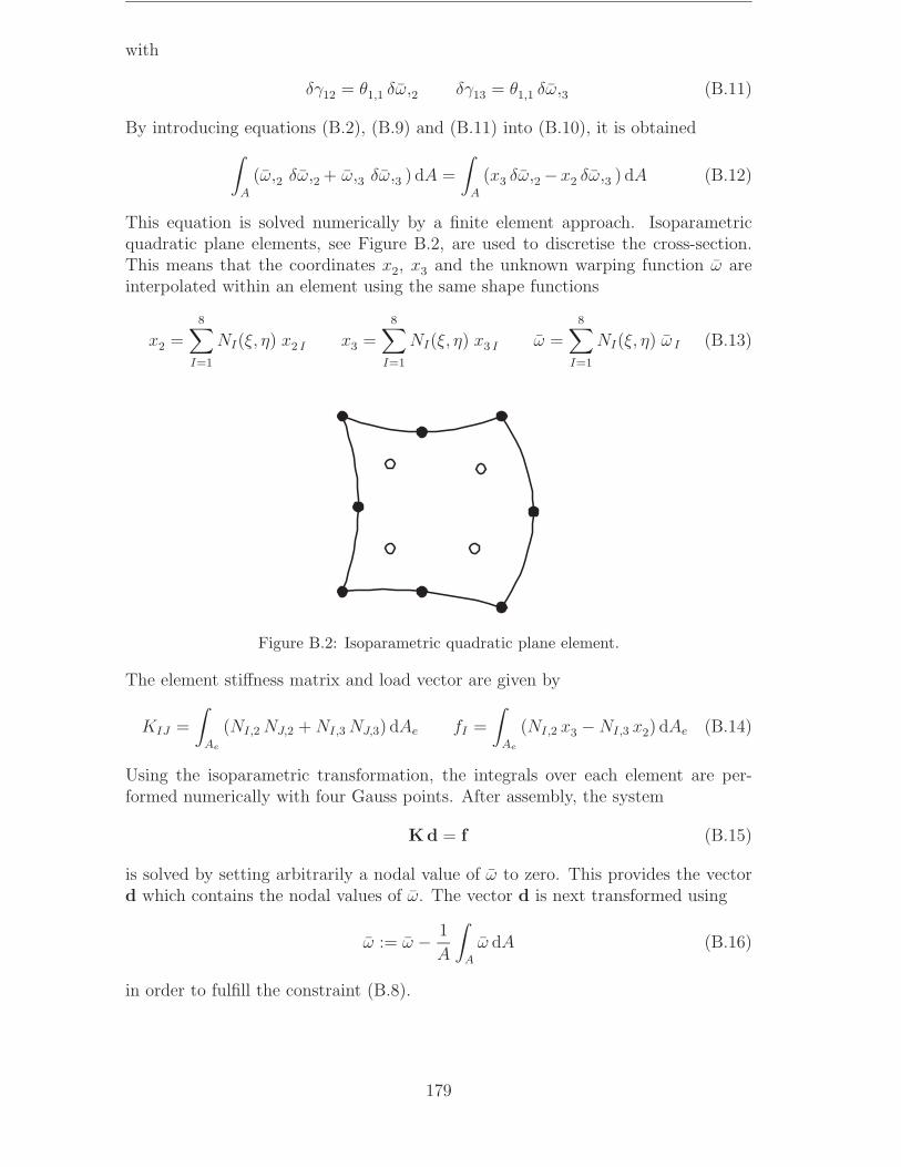
with

δγ12 = θ1,1 δω,2 δγ13 = θ1,1 δω,3 (B.11)

By introducing equations (B.2), (B.9) and (B.11) into (B.10), it is obtained∫A

(ω,2 δω,2 + ω,3 δω,3 ) dA =

∫A

(x3 δω,2 −x2 δω,3 ) dA (B.12)

This equation is solved numerically by a finite element approach. Isoparametricquadratic plane elements, see Figure B.2, are used to discretise the cross-section.This means that the coordinates x2, x3 and the unknown warping function ω areinterpolated within an element using the same shape functions

x2 =8∑

I=1

NI(ξ, η) x2 I x3 =8∑

I=1

NI(ξ, η) x3 I ω =8∑

I=1

NI(ξ, η) ω I (B.13)

Figure B.2: Isoparametric quadratic plane element.

The element stiffness matrix and load vector are given by

KIJ =

∫Ae

(NI,2 NJ,2 + NI,3 NJ,3) dAe fI =

∫Ae

(NI,2 x3 − NI,3 x2) dAe (B.14)

Using the isoparametric transformation, the integrals over each element are per-formed numerically with four Gauss points. After assembly, the system

Kd = f (B.15)

is solved by setting arbitrarily a nodal value of ω to zero. This provides the vectord which contains the nodal values of ω. The vector d is next transformed using

ω := ω − 1

A

∫A

ω dA (B.16)

in order to fulfill the constraint (B.8).

179

B.4 Cross-section quantities

The cross-section quantities defined in equations (4.130), and those introduced inthe present section, are integrated numerically using 4 Gauss points for each isopara-metric elements.

The coordinates of the shear center are derived from the two last (B.6) equations,which gives after some work

c2 = − Iω3 I22 − Iω2 I23

I22 I33 − I 223

c3 =Iω2 I33 − Iω3 I23

I22 I33 − I 223

(B.17)

with

Iω2 =

∫A

ω x2 dA Iω3 =

∫A

ω x3 dA (B.18)

The Saint-Venant torsion modulus, defined in equation (4.129), can be calculateddirectly by

J = I22 + I33 − dT f (B.19)

with d and f defined in (B.15).

Finally, Iω and Iωr are rewritten with the help of equation (B.7) as

Iω =

∫A

ω 2 dA − I33 c 22 − I22 c 2

3 + 2 I23 c2 c3 (B.20a)

Iωr =

∫A

ωr2 dA + I3r c2 − I2r c3 (B.20b)

180