Co-Optimization of Design and Fabrication Plans for Carpentry

Co-Optimization of Design and Fabrication Plans for Carpentry

HAISEN ZHAO, University of Washington and Shandong UniversityMAX WILLSEY, University of WashingtonAMY ZHU, University of WashingtonCHANDRAKANA NANDI, University of WashingtonZACHARY TATLOCK, University of WashingtonJUSTIN SOLOMON,Massachusetts Institute of TechnologyADRIANA SCHULZ, University of Washington

5

7

9

11

13

15

24 27 30 33 36 39 42 45 48

Fab

rica

tio

n T

ime

(min

)

Material Cost (dollar)

5

7

9

11

13

15

24 27 30 33 36 39 42 45 48

Fab

rica

tio

n T

ime

(min

)

Material Cost (dollar)

(a) (b)

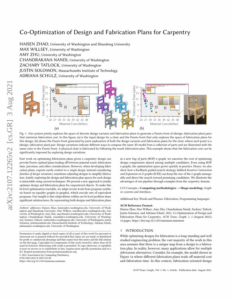
Fig. 1. Our system jointly explores the space of discrete design variants and fabrication plans to generate a Pareto front of (design, fabrication plan) pairsthat minimize fabrication cost. In this figure, (a) is the input design for a chair and the Pareto front that only explores the space of fabrication plans forthis design, (b) shows the Pareto front generated by joint exploration of both the design variants and fabrication plans for the chair, where each point is a(design, fabrication plan) pair. Design variations indicate different ways to compose the same 3D model from a collection of parts and are illustrated with thesame color in the Pareto front. A physical chair is fabricated by following the result fabrication plan. This example shows that the fabrication cost can besignificantly improved by exploring design variations.

Past work on optimizing fabrication plans given a carpentry design canprovide Pareto-optimal plans trading off between material waste, fabricationtime, precision, and other considerations. However, when developing fabri-cation plans, experts rarely restrict to a single design, instead consideringfamilies of design variations, sometimes adjusting designs to simplify fabrica-tion. Jointly exploring the design and fabrication plan spaces for each designis intractable using current techniques. We present a new approach to jointlyoptimize design and fabrication plans for carpentered objects. To make thisbi-level optimization tractable, we adapt recent work from program synthe-sis based on equality graphs (e-graphs), which encode sets of equivalentprograms. Our insight is that subproblems within our bi-level problem sharesignificant substructures. By representing both designs and fabrication plans

Authors’ addresses: Haisen Zhao, [email protected], University of Wash-ington and Shandong University; Max Willsey, [email protected], Uni-versity of Washington; Amy Zhu, [email protected], University of Wash-ington; Chandrakana Nandi, [email protected], University of Washing-ton; Zachary Tatlock, [email protected], University of Washington; JustinSolomon, [email protected], Massachusetts Institute of Technology; Adriana Schulz,[email protected], University of Washington.

Permission to make digital or hard copies of all or part of this work for personal orclassroom use is granted without fee provided that copies are not made or distributedfor profit or commercial advantage and that copies bear this notice and the full citationon the first page. Copyrights for components of this work owned by others than ACMmust be honored. Abstracting with credit is permitted. To copy otherwise, or republish,to post on servers or to redistribute to lists, requires prior specific permission and/or afee. Request permissions from [email protected].© 2021 Association for Computing Machinery.0730-0301/2021/8-ART $15.00https://doi.org/10.1145/nnnnnnn.nnnnnnn

in a new bag of parts (BOP) e-graph, we amortize the cost of optimizingdesign components shared among multiple candidates. Even using BOPe-graphs, the optimization space grows quickly in practice. Hence, we alsoshow how a feedback-guided search strategy dubbed Iterative Contractionand Expansion on E-graphs (ICEE) can keep the size of the e-graph manage-able and direct the search toward promising candidates. We illustrate theadvantages of our pipeline through examples from the carpentry domain.

CCS Concepts: •Computingmethodologies→ Shapemodeling; Graph-ics systems and interfaces.

Additional Key Words and Phrases: Fabrication, Programming languages

ACM Reference Format:Haisen Zhao, Max Willsey, Amy Zhu, Chandrakana Nandi, Zachary Tatlock,Justin Solomon, and Adriana Schulz. 2021. Co-Optimization of Design andFabrication Plans for Carpentry. ACM Trans. Graph. 1, 1 (August 2021),14 pages. https://doi.org/10.1145/nnnnnnn.nnnnnnn

1 INTRODUCTIONWhile optimizing designs for fabrication is a long-standing and wellstudied engineering problem, the vast majority of the work in thisarea assumes that there is a unique map from a design to a fabrica-tion plan. In reality, however, many applications allow for multiplefabrication alternatives. Consider, for example, the model shown inFigure 1a where different fabrication plans trade off material costand fabrication time. In this context, fabrication-oriented design

ACM Trans. Graph., Vol. 1, No. 1, Article . Publication date: August 2021.

arX

iv:2

107.

1226

5v2

[cs

.GR

] 3

Aug

202

1

https://doi.org/10.1145/nnnnnnn.nnnnnnn

https://doi.org/10.1145/nnnnnnn.nnnnnnn

2 • Haisen Zhao, Max Willsey, Amy Zhu, Chandrakana Nandi, Zachary Tatlock, Justin Solomon, and Adriana Schulz

optimization becomes even more challenging, since it requires ex-ploring the landscape of optimal fabrication plans for many designvariations. Every variation of the original design (Figure 1b) de-termines a new landscape of fabrication plans with different costtrade-offs. Designers must therefore navigate the joint space of de-sign and fabrication plans to find the optimal landscape of solutions.In this work, we present a novel approach that simultaneously

optimizes both the design and fabrication plans for carpentry. Priorwork represents carpentry designs and fabrication plans as programs[Wu et al. 2019] to optimize the fabrication plan of a single design ata time. Our approach also uses a program-like representation, butwe jointly optimize the design and the fabrication plan.

Our problem setting has two main challenges. First, the discretespace of fabrication plan alternatives can vary significantly for eachdiscrete design variation. This setup can be understood as a bi-levelproblem, characterized by the existence of two optimization prob-lems in which the constraint region of the upper-level problem (thejoint space of designs and fabrication plans) is implicitly determinedby the lower-level optimization problem (the space of feasible fab-rication plans given a design). The second challenge is that thereare multiple conflicting fabrication objectives. Plans that improvethe total production time may waste more material or involve lessprecise cutting operations. Our goal is therefore to find multiplesolutions to our fabrication problem that represent optimal pointsin the landscape of possible trade-offs, called the Pareto front. Im-portantly, the different fabrication plans on the Pareto front maycome from different design variations. The complexity of the bi-level search space combined with the need for finding a landscapeof Pareto-optimal solutions makes this optimization challenging.We propose a method to make this problem computationally

tractable in light of the challenges above. Our key observation isthat there is redundancy on both levels of the search space that canbe exploited. In particular, different design variations may sharesimilar subsets of parts, which can use the same fabrication plans.We propose exploiting this sharing to encode a large number ofdesign variations and their possible fabrication plans compactly. Weuse a data structure called an equivalence graph (e-graph) [Nelson1980] to maximize sharing and thus amortize the cost of heavilyoptimizing part of a design since all other design variations sharinga part benefit from its optimization.E-graphs have been growing in popularity in the programming

languages community; they provide a compact representation forequivalent programs that can be leveraged for theorem proving andcode optimization. There are two challenges in directly applying e-graphs to design optimization under fabrication variations, detailedbelow.First, the different fabrication plans for a given design are all

semantically equivalent programs. However, the fabrication plansassociated with different design variations, in general, are not se-mantically equivalent, i.e., they may produce different sets of parts.This makes it difficult to directly apply traditional techniques whichexploit sharing by searching for minimal cost, but still semanticallyequivalent, versions of a program. One of our key technical contri-butions is therefore a new data structure for representing the searchspace, which we call the Bag-of-Parts (BOP) E-graph. This datastructure takes advantage of common substructures across both

design and fabrication plans to maximize redundancy and boost theexpressive power of e-graphs.

Second, optimization techniques built around e-graphs have adopteda two stage approach: expansion (incrementally growing the e-graphby including more equivalent programs1) followed by extraction(the process of searching the e-graph for an optimal program). Inparticular, the expansion stage has not been feedback-directed, i.e.,the cost of candidate programs has only been used in extraction, butthat information has not been fed back in to guide further e-graphexpansion. A key contribution of our work is a method for IterativeContraction and Expansion on E-graphs (ICEE). Because ICEEis feedback-directed, it enables us to effectively explore the largecombinatorial space of designs and their corresponding fabricationplans. ICEE also uses feedback to prune the least valuable parts ofthe e-graph during search, keeping its size manageable. Further,these expansion and contraction decisions are driven by a multi-objective problem that enables finding a diverse set of points on thePareto front.We implemented our approach and compared it against prior

work and against results generated by carpentry experts. Our resultsshow that ICEE is up to 17× faster than prior approaches whileachieving similar results. In some cases, it is the only approach thatsuccessfully generates an optimal set of results due to its efficiencyin exploring large design spaces. We showcase how our method canbe applied to a variety of designs of different complexity and showhow our method is advantageous in diverse contexts. For examplewe achieve 25% reduced material in one model, 60% reduced timein another, and 20% saved total cost in a third when assuming acarpenter charges $40/h, when compared to a method that does notexplore design variations.

2 RELATED WORKOptimization for Design and Fabrication. Design for fabrication

is an exciting area of research that aims to automatically achievedesired properties while optimizing fabrication plans. Examples ofrecent work include computational design of glass façades [Gavriilet al. 2020], compliantmechanical systems [Tang et al. 2020], barcodeembeddings [Maia et al. 2019], and interlocking assemblies [Cignoniet al. 2014; Hildebrand et al. 2013; Wang et al. 2019], among manyothers [Bickel et al. 2018; Schwartzburg and Pauly 2013]. Fabricationconsiderations are typically taken into account as constraints duringdesign optimization, but these methods assume that there is an algo-rithm for generating one fabrication plan for a given design. To thebest of our knowledge, no prior work explores the multi-objectivespace of fabrication alternatives during design optimization.There is also significant literature on fabrication plan optimiza-

tion for a given design under different constraints. Recent workincludes optimization of composite molds for casting [Alderighiet al. 2019], tool paths for 3D printing [Etienne et al. 2019; Zhao et al.2016], and decomposition for CNC milling [Mahdavi-Amiri et al.2020; Yang et al. 2020]. While some of these methods minimize thedistance to a target design under fabrication constraints [Duenseret al. 2020; Zhang et al. 2019], none of them explores a space ofdesign modification to minimize fabrication cost.

1In the programming languages literature, this is known as equality saturation.


Co-Optimization of Design and Fabrication Plans for Carpentry • 3

In contrast, our work jointly explores the design and fabricationspace in the carpentry domain, searching for the Pareto-optimaldesign variations that minimize multiple fabrication costs.

Design and Fabrication for Carpentry. Carpentry is a well-studieddomain in design and fabrication due to its wide application scope.Prior work has investigated interactive and optimization methodsfor carpentry design [Fu et al. 2015; Garg et al. 2016; Koo et al.2014; Song et al. 2017; Umetani et al. 2012]. There is also a body ofwork on fabrication plan optimization [Koo et al. 2017; Lau et al.2011; Leen et al. 2019; Yang et al. 2015]. Closest to our work isthe system of Wu et al. [2019], which represents both carpentrydesigns and fabrication plans as programs and introduces a compilerthat optimizes fabrication plans for a single design. While our workbuilds on the domain specific languages (DSLs) proposed in thatprior work, ours is centered on the fundamental problem of designoptimization under fabrication alternatives, which has not beenpreviously addressed.

Bi-Level Multi-Objective Optimization. Our problem and otherslike it are bi-level, with a nested structure in which each designdetermines a different space of feasible fabrication plans. The great-est challenge in handling bi-level problems lies in the fact that thelower level problem determines the feasible space of the upper leveloptimization problem. More background on bi-level optimizationcan be found in the book by Dempe [2018], as well as review papersby Lu et al. [2016] and Sinha et al. [2017].

Bi-level problems with multiple objectives can be even more chal-lenging to solve [Dempe 2018]. Some specific cases are solved withclassical approaches, such as numerical optimization [Eichfelder2010] and the 𝜖-constraint method [Shi and Xia 2001]. Heuristic-driven search techniques have been used to address bi-level multi-objective problems, such as genetic algorithms [Yin 2000] and parti-cle swarm optimization [Halter and Mostaghim 2006]. These meth-ods apply a heuristic search to both levels in a nestedmanner, search-ing over the upper level with NSGA-II operations, while the evalu-ating each individual call in a low-level NSGA-II process [Deb andSinha 2009]. Our ICEE framework also applies a genetic algorithmduring search. Different from past techniques, ICEE does not nestthe two-level search but rather reuses structure between differentupper-level feasible points. ICEE jointly explores both the designand fabrication spaces using the BOP E-graph representation.

E-graphs. An e-graph is an efficient data structure for compactlyrepresenting large sets of equivalent programs. E-graphs were orig-inally developed for automated theorem proving [Nelson 1980],and were first adapted for program optimization by Joshi et al.[2002]. These ideas were further expanded to handle programs withloops and conditionals [Tate et al. 2009] and applied to a varietyof domains for program optimization, synthesis, and equivalencechecking [Nandi et al. 2020; Panchekha et al. 2015; Premtoon et al.2020; Stepp et al. 2011; Wang et al. 2020; Willsey et al. 2021; Wuet al. 2019].

Recently, e-graphs have been used for optimizing designs [Nandiet al. 2020], and also for optimizing fabrication plans [Wu et al.2019], but they have not been used to simultaneously optimize bothdesigns and fabrication plans. Prior work also does not explore

feedback-driven e-graph expansion and contraction for managinglarge optimization search spaces.

3 BACKGROUNDIn this section, we introduce some mathematical preliminaries usedin the rest of the paper.

3.1 Multi-Objective OptimizationA multi-objective optimization problem is defined by set of objec-tives 𝑓𝑖 : x ↦→ R that assign a real value to each point x ∈ X inthe feasible search space X. We choose the convention that smallvalues of 𝑓𝑖 (x) are desirable for objective 𝑓𝑖 .

As these objectives as typically conflicting, our algorithm searchesfor a diverse set of points that represent optimal trade-offs, calledPareto optimal [Deb 2014]:

Definition 3.1 (Pareto optimality). A point x ∈ X is Pareto optimalif there does not exist any x′ ∈ X so that 𝑓𝑖 (x) ≥ 𝑓𝑖 (x′) for all 𝑖 and𝑓𝑖 (x) > 𝑓𝑖 (x′) for at least one 𝑖 .We use 𝐹 : x ↦→ R𝑁 to denote the concatenation (𝑓1 (x), . . . , 𝑓𝑁 (x)).

Pareto optimal points are the solution to the multi-objective opti-mization:

minx𝐹 (x) s.t. x ∈ X. (1)

The image of all Pareto-optimal points is called the Pareto front.

Non-Dominated Sorting. Genetic algorithms based on non-dominatedsorting are a classic approach to multi-objective optimization [Deband Jain 2013; Deb et al. 2002]. The key idea is that sorting should bedone based on proximity to the Pareto front. These papers define theconcept of Pareto layers, where layer 0 is the Pareto front, and layer𝑙 is the Pareto front that would result if all solutions from layers 0to 𝑙 − 1 are removed. When selecting parent populations or whenpruning children populations, solutions in lower layers are addedfirst, and when a layer can only be added partially, elements of thislayer are chosen to increase diversity. Different variations of thismethod use different strategies for diversity; we use NSGA-III [Deband Jain 2013] in our work.

Hypervolume. Hypervolume [Auger et al. 2009] is a metric com-monly used to compare two sets of image points during Paretofront discovery. To calculate the hypervolume, we draw the smallestrectangular prism (axis-aligned, as per the 𝐿1 norm) between somereference point and each point on the pareto front. We then unionthe volume of each shape to calculate the hypervolume. Thus, alarger hypervolume implies a better approximation of the Paretofront.

3.2 Bi-level Multi-Objective OptimizationGiven a design space D that defines possible variations of a carpen-try model, our goal is to find a design 𝑑 ∈ D and a correspondingfabrication plan 𝑝 ∈ P𝑑 that minimizes a vector of conflicting objec-tives, where P𝑑 is the space of fabrication plans corresponding todesign 𝑑 . This setup yields the following multi-objective optimiza-tion problem:

min𝑝,𝑑

𝐹 (𝑑, 𝑝) s.t. 𝑑 ∈ D, 𝑝 ∈ P𝑑



where P𝑑 defines the space of all possible plans for fabricationthe design 𝑑 . Generally, our problem can be expressed as a bi-levelmulti-objective optimization that searches across designs to findthose with the best fabrication costs, and requires optimizing thefabrication for each design during this exploration [Lu et al. 2016]:

min𝑑

𝐹 (𝑑, 𝑝) s.t. 𝑑 ∈ D, 𝑝 = argmin𝑝

𝐹 (𝑑, 𝑝)

where argmin refers to Pareto-optimal solutions to themulti-objectiveoptimization problem.

A naïve solution to this bi-level problem would be to search overthe design space D using a standard multi-objective optimizationmethod, while solving the nested optimization problem to find thefabrication plans given a design at each iteration. Given the com-binatorial nature of our domain, this would be prohibitively slow,which motivates our proposed solution.

3.3 Equivalence Graphs (E-graphs)Typically, programs (often referred to as terms) are viewed as tree-like structures containing smaller sub-terms. For example, the term3 × 2 has the operator × at its “root” and two sub-terms, 3 and 2,each of which has no sub-terms. Terms can be expressed in mul-tiple syntactically different ways. For example, in the language ofarithmetic, the term 3 × 2 is semantically equivalent to 3 + 3, butthey are syntactically different. Naïvely computing and storing allsemantically equivalent but syntactically different variants of the aterm requires exponential time and memory. For a large program,this makes searching the space of equivalent terms intractable.

E-graphs [Nelson 1980] are designed to address this challenge—ane-graph is a data structure that represents many equivalent termsefficiently by sharing sub-terms whenever possible. An e-graph notonly stores a large set of terms, but it represents an equivalencerelation over those terms, i.e., it partitions the set of terms intoequivalence classes, or e-classes, each of which contains semanticallyequivalent but syntactically distinct terms. In Section 4.2, we showhow to express carpentry designs in a way that captures the benefitsof the e-graph.

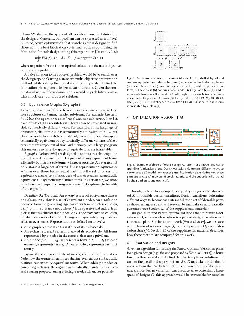
Definition 3.2 (E-graph). An e-graph is a set of equivalence classesor e-classes. An e-class is a set of equivalent e-nodes. An e-node is anoperator from the given language paired with some e-class children,i.e., 𝑓 (𝑐1, . . . , 𝑐𝑛) is an e-nodewhere 𝑓 is an operator and each 𝑐𝑖 is ane-class that is a child of this e-node. An e-node may have no children,in which case we call it a leaf. An e-graph represents an equivalencerelation over terms. Representation is defined recursively:• An e-graph represents a term if any of its e-classes do.• An e-class represents a term if any of its e-nodes do. All termsrepresented by e-nodes in the same e-class are equivalent.

• An e-node 𝑓 (𝑐1, . . . , 𝑐𝑛) represents a term 𝑓 (𝑡1, . . . , 𝑡𝑛) if eache-class 𝑐𝑖 represents term 𝑡𝑖 . A leaf e-node 𝑔 represents just thatterm 𝑔.Figure 2 shows an example of an e-graph and representation.

Note how the e-graph maximizes sharing even across syntacticallydistinct, semantically equivalent terms. When adding e-nodes orcombining e-classes, the e-graph automatically maintains this maxi-mal sharing property, using existing e-nodes whenever possible.

+

3

*

2

+

(a)

(b)

(c) (d)

+ 4(e)

Fig. 2. An example e-graph. E-classes (dotted boxes labelled by letters)contain equivalent e-nodes (solid boxed) which refer to children e-classes(arrows). The e-class (c) contains one leaf e-node, 3, and it represents oneterm, 3. The e-class (b) contains two e-nodes, (c) + (c) and (c) ∗ (d), and itrepresents two terms: 3+ 3 and 3 ∗ 2. Although the e-class (a) only containsone e-node, it represents 4 terms: (3+3) + (2+2) , (3∗2) + (2+2) , (3+3) +4,and (3 ∗ 2) + 4. If + is cheaper than ∗, then (3 + 3) + 4 is the cheapest termrepresented by e-class (a).

4 OPTIMIZATION ALGORITHM

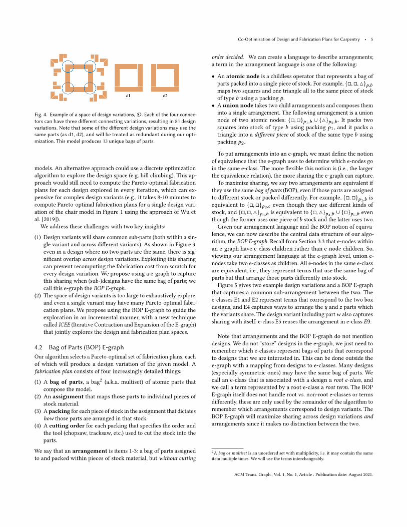
Fig. 3. Example of three different design variations of a model and corre-sponding fabrication plans. Design variations determine different ways todecompose a 3Dmodel into a set of parts. Fabrication plans define how theseparts are arranged in pieces of stock material and the cut order (illustratedby the numbers along each cut).

Our algorithm takes as input a carpentry design with a discreteset D of possible design variations. Design variations determinedifferent ways to decompose a 3Dmodel into a set of fabricable parts,as shown in Figures 3 and 4. These can be manually or automaticallygenerated (see Section 1.1 of the supplemental material).Our goal is to find Pareto-optimal solutions that minimize fabri-

cation cost, where each solution is a pair of design variation andfabrication plan. Similar to prior work [Wu et al. 2019], we measurecost in terms of material usage (𝑓𝑐 ), cutting precision (𝑓𝑝 ), and fabri-cation time (𝑓𝑡 ). Section 1.3 of the supplemental material describeshow these metrics are computed for this work.

4.1 Motivation and InsightsGiven an algorithm for finding the Pareto-optimal fabrication plansfor a given design (e.g., the one proposed byWu et al. [2019]), a bruteforce method would simply find the Pareto-optimal solutions foreach of the possible design variations 𝑑 ∈ D and take the dominantones to form the Pareto front of the combined design/fabricationspace. Since design variations can produce an exponentially largespace of designs D, this approach would be intractable for complex



Fig. 4. Example of a space of design variations, D. Each of the four connec-tors can have three different connecting variations, resulting in 81 designvariations. Note that some of the different design variations may use thesame parts (as d1, d2), and will be treated as redundant during our opti-mization. This model produces 13 unique bags of parts.

models. An alternative approach could use a discrete optimizationalgorithm to explore the design space (e.g. hill climbing). This ap-proach would still need to compute the Pareto-optimal fabricationplans for each design explored in every iteration, which can ex-pensive for complex design variants (e.g., it takes 8-10 minutes tocompute Pareto-optimal fabrication plans for a single design vari-ation of the chair model in Figure 1 using the approach of Wu etal. [2019]).We address these challenges with two key insights:

(1) Design variants will share common sub-parts (both within a sin-gle variant and across different variants). As shown in Figure 3,even in a design where no two parts are the same, there is sig-nificant overlap across design variations. Exploiting this sharingcan prevent recomputing the fabrication cost from scratch forevery design variation. We propose using a e-graph to capturethis sharing when (sub-)designs have the same bag of parts; wecall this e-graph the BOP E-graph.

(2) The space of design variants is too large to exhaustively explore,and even a single variant may have many Pareto-optimal fabri-cation plans. We propose using the BOP E-graph to guide theexploration in an incremental manner, with a new techniquecalled ICEE (Iterative Contraction and Expansion of the E-graph)that jointly explores the design and fabrication plan spaces.

4.2 Bag of Parts (BOP) E-graphOur algorithm selects a Pareto-optimal set of fabrication plans, eachof which will produce a design variation of the given model. Afabrication plan consists of four increasingly detailed things:

(1) A bag of parts, a bag2 (a.k.a. multiset) of atomic parts thatcompose the model.

(2) An assignment that maps those parts to individual pieces ofstock material.

(3) A packing for each piece of stock in the assignment that dictateshow those parts are arranged in that stock.

(4) A cutting order for each packing that specifies the order andthe tool (chopsaw, tracksaw, etc.) used to cut the stock into theparts.

We say that an arrangement is items 1-3: a bag of parts assignedto and packed within pieces of stock material, but without cutting

order decided. We can create a language to describe arrangements;a term in the arrangement language is one of the following:

• An atomic node is a childless operator that represents a bag ofparts packed into a single piece of stock. For example, {□,□, △}𝑝,𝑏maps two squares and one triangle all to the same piece of stockof type 𝑏 using a packing 𝑝 .

• A union node takes two child arrangements and composes theminto a single arrangement. The following arrangement is a unionnode of two atomic nodes: {□,□}𝑝1,𝑏 ∪ {△}𝑝2,𝑏 . It packs twosquares into stock of type 𝑏 using packing 𝑝1, and it packs atriangle into a different piece of stock of the same type 𝑏 usingpacking 𝑝2.

To put arrangements into an e-graph, we must define the notionof equivalence that the e-graph uses to determine which e-nodes goin the same e-class. The more flexible this notion is (i.e., the largerthe equivalence relation), the more sharing the e-graph can capture.

To maximize sharing, we say two arrangements are equivalent ifthey use the same bag of parts (BOP), even if those parts are assignedto different stock or packed differently. For example, {□,□}𝑝1,𝑏 isequivalent to {□,□}𝑝2,𝑐 even though they use different kinds ofstock, and {□,□, △}𝑝3,𝑏 is equivalent to {□, △}𝑝4,𝑏 ∪ {□}𝑝5,𝑏 eventhough the former uses one piece of 𝑏 stock and the latter uses two.

Given our arrangement language and the BOP notion of equiva-lence, we can now describe the central data structure of our algo-rithm, the BOP E-graph. Recall from Section 3.3 that e-nodes withinan e-graph have e-class children rather than e-node children. So,viewing our arrangement language at the e-graph level, union e-nodes take two e-classes as children. All e-nodes in the same e-classare equivalent, i.e., they represent terms that use the same bag ofparts but that arrange those parts differently into stock.

Figure 5 gives two example design variations and a BOP E-graphthat captures a common sub-arrangement between the two. Thee-classes E1 and E2 represent terms that correspond to the two boxdesigns, and E4 captures ways to arrange the 𝑦 and 𝑧 parts whichthe variants share. The design variant including part𝑤 also capturessharing with itself: e-class E5 reuses the arrangement in e-class 𝐸9.

Note that arrangements and the BOP E-graph do not mentiondesigns. We do not “store” designs in the e-graph, we just need toremember which e-classes represent bags of parts that correspondto designs that we are interested in. This can be done outside thee-graph with a mapping from designs to e-classes. Many designs(especially symmetric ones) may have the same bag of parts. Wecall an e-class that is associated with a design a root e-class, andwe call a term represented by a root e-class a root term. The BOPE-graph itself does not handle root vs. non-root e-classes or termsdifferently, these are only used by the remainder of the algorithm toremember which arrangements correspond to design variants. TheBOP E-graph will maximize sharing across design variations andarrangements since it makes no distinction between the two.

2A bag or multiset is an unordered set with multiplicity, i.e. it may contain the sameitem multiple times. We will use the terms interchangeably.



E1: { }

U1z

y

y

x

yw

z

w

E2: { }

U2

E3: { }

U3

E4: { }

U4

E5: { }

U5

E6: { } E7: { } E8: { } E9: { }

x y z wy y z w

x y y z w w

x y z w

A11A10A9A8

A4 A5 A6 A7

A2 A3A1

(a)

(b)

(c) A4 x y A9 y A10 z

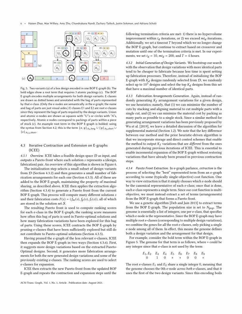
Fig. 5. Two variants (a) of a box design encoded in one BOP E-graph (b). Thebold edges show a root term that requires 3 atomic packings (c). The BOPE-graph encodes multiple arrangements for both design variants. E-classesare drawn as dotted boxes and annotated with the bag of parts representedby that e-class. (Only the e-nodes are semantically in the e-graph; the nameand bag of parts are just visual aides.) E-classes E1 and E2 are root e-classessince they represent the bags of parts required by the design variants. Unionand atomic e-nodes are shown as squares with “U”s or circles with “A”s,respectively. Atomic e-nodes correspond to packings of parts within a pieceof stock (c). An example root term in the BOP E-graph is bolded; usingthe syntax from Section 4.2, this is the term {𝑥, 𝑦 }𝐴4,long ∪ {𝑦 }𝐴9,short ∪{𝑧 }𝐴10,short.

4.3 Iterative Contraction and Extension on E-graphs(ICEE)

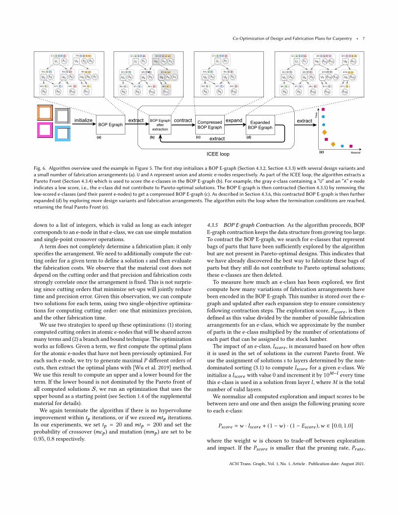
4.3.1 Overview. ICEE takes a feasible design space D as input, andoutputs a Pareto front where each solution 𝑠 represents a (design,fabrication) pair. An overview of this algorithm is shown in Figure 6.The initialization step selects a small subset of design variants

from D (Section 4.3.2) and then generates a small number of fab-rication arrangements for each one (Section 4.3.3). All of these areadded to the BOP E-graph, maintaining the property of maximalsharing, as described above. ICEE then applies the extraction algo-rithm (Section 4.3.4) to generate a Pareto front from the currentBOP E-graph. This process will compute many different solutions 𝑠and their fabrication costs 𝐹 (𝑠) = (𝑓𝑚 (𝑠), 𝑓𝑝 (𝑠), 𝑓𝑡 (𝑠)), all of whichare stored in the solution set S.The resulting Pareto front is used to compute ranking scores

for each e-class in the BOP E-graph; the ranking score measureshow often this bag of parts is used in Pareto-optimal solutions andhow many fabrication variations have been explored for this bagof parts. Using these scores, ICEE contracts the BOP E-graph bypruning e-classes that have been sufficiently explored but still donot contribute to Pareto-optimal solutions (Section 4.3.5).Having pruned the e-graph of the less relevant e-classes, ICEE

then expands the BOP E-graph in two ways (Section 4.3.6). First,it suggests more design variations based on the extracted Pareto-Optimal designs. Second, it generates more fabrication arrange-ments for both the new generated design variations and some of thepreviously existing e-classes. The ranking scores are used to selecte-classes for expansion.ICEE then extracts the new Pareto front from the updated BOP

E-graph and repeats the contraction and expansion steps until the

following termination criteria are met: 1) there is no hypervolumeimprovement within 𝑡𝑑 iterations, or 2) we exceed𝑚𝑡𝑑 iterations.Additionally, we set a timeout𝑇 beyond which we no longer changethe BOP E-graph, but continue to extract based on crossover andmutation until one of the termination criteria is met. In our experi-ments, we set 𝑡𝑑 = 10,𝑚𝑡𝑑 = 200, and 𝑇 = 4 hours.

4.3.2 Initial Generation of Design Variants. We bootstrap our searchwith the observation that design variations with more identical partstend to be cheaper to fabricate because less time is spent settingup fabrication processes. Therefore, instead of initializing the BOPE-graph with 𝐾𝑑 designs randomly selected from D, we randomlyselect up to 105 designs and select the top 𝐾𝑑 designs from this setthat have a maximal number of identical parts.

4.3.3 Fabrication Arrangements Generation. Again, instead of ran-domly generating 𝐾𝑓 arrangement variations for a given design,we use heuristics; namely, that (1) we can minimize the number ofcuts by stacking and aligning material to cut multiple parts with asingle cut, and (2) we can minimize the material cost by packing asmany parts as possible to a single stock. Since a similar method forgenerating arrangement variations has been previously proposed byWu et al. [2019], we leave a detailed discussion of the algorithm forsupplemental material (Section 1.2). We note that the key differencebetween our method and the prior heuristic-driven algorithm isthat we incorporate storage and direct control schemes that enablethe method to output 𝐾𝑓 variations that are different from the onesgenerated during previous iterations of ICEE. This is essential toenable incremental expansion of the BOP E-graph without restoringvariations that have already been pruned in previous contractionsteps.

4.3.4 Pareto Front Extraction. In e-graph parlance, extraction is theprocess of selecting the “best” represented term from an e-graphaccording to some (typically single-objective) cost function. Oneway to view extraction is that it simply chooses which e-node shouldbe the canonical representative of each e-class; once that is done,each e-class represents a single term. Since our cost function is multi-objective, we must instead extract a set of terms (arrangements)from the BOP E-graph that forms a Pareto front.

We use a genetic algorithm [Deb and Jain 2013] to extract termsfrom the BOP E-graph. The population size is set to 𝑁𝑝𝑜𝑝 . Thegenome is essentially a list of integers, one per e-class, that specifieswhich e-node is the representative. Since the BOP E-graph may havemultiple root e-classes (corresponding to multiple design variations),we combine the genes for all the root e-classes, only picking a singlee-node among all of them. In effect, this means the genome definesboth a design variation and the arrangement for that design.For example, consider the bold term within the BOP E-graph in

Figure 5. The genome for that term is as follows, where ∗ could beany integer since that e-class is not used by the term:

𝐸1, 𝐸2 𝐸3 𝐸4 𝐸5 𝐸6 𝐸7 𝐸8 𝐸90 1 0 ∗ ∗ 0 0 ∗

The root e-classes 𝐸1 and 𝐸2 share a single integer 0, meaning thatthe genome chooses the 0th e-node across both e-classes, and that ituses the first of the two design variants. Since this encoding boils



initialize extract contract expand extract

extract

BOP EgraphBOP Egraph

afterextraction

CompressedBOP Egraph

ExpandedBOP Egraph

(a) (b) (c) (d)

(e) Material

Tim

e

ICEE loop

A1U1 U2

E1:{ }x y y z

A4U3

E3:{ }x y

A5U4

E4:{ }y z

A2 A3

E2:{ }y z w w

U5 A6 A7

E5:{ }w w

A9

E7:{ }

A8

E6:{ }x

A10

E8:{ }

A11

E9:{ }y z w

A1U1 U2

E1:{ }x y y z

A4U3

E3:{ }x y

A5U4

E4:{ }y z

A2 A3

E2:{ }y z w w

U5 A6 A7

E5:{ }w w

A9

E7:{ }

A8

E6:{ }x

A10

E8:{ }

A11

E9:{ }y z w

A1U1

E1:{ }x y y z

A4U3

E3:{ }x y

A5U4

E4:{ }y z

A9

E7:{ }

A8

E6:{ }x

A10

E8:{ }y z

A1U1 U6

E1:{ }x y y z

A4U3

E3:{ }x y

A5U4

E4:{ }y z

A12 A13

E9:{ }y z T

U7 A14 A15

E10:{ }

A9

E7:{ }

A8

E6:{ }x

A10

E8:{ }

A16

E11:{ }Ty z

T

T T

U8 A17

E9:{ }T T S S

U9 A18

E10:{ }S S

A16

E11:{ }S

Fig. 6. Algorithm overview used the example in Figure 5. The first step initializes a BOP E-graph (Section 4.3.2, Section 4.3.3) with several design variants anda small number of fabrication arrangements (a). U and A represent union and atomic e-nodes respectively. As part of the ICEE loop, the algorithm extracts aPareto Front (Section 4.3.4) which is used to score the e-classes in the BOP E-graph (b). For example, the gray e-class containing a “U” and an “A” e-nodeindicates a low score, i.e., the e-class did not contribute to Pareto-optimal solutions. The BOP E-graph is then contracted (Section 4.3.5) by removing thelow-scored e-classes (and their parent e-nodes) to get a compressed BOP E-graph (c). As described in Section 4.3.6, this contracted BOP E-graph is then furtherexpanded (d) by exploring more design variants and fabrication arrangements. The algorithm exits the loop when the termination conditions are reached,returning the final Pareto Front (e).

down to a list of integers, which is valid as long as each integercorresponds to an e-node in that e-class, we can use simple mutationand single-point crossover operations.

A term does not completely determine a fabrication plan; it onlyspecifies the arrangement. We need to additionally compute the cut-ting order for a given term to define a solution 𝑠 and then evaluatethe fabrication costs. We observe that the material cost does notdepend on the cutting order and that precision and fabrication costsstrongly correlate once the arrangement is fixed. This is not surpris-ing since cutting orders that minimize set-ups will jointly reducetime and precision error. Given this observation, we can computetwo solutions for each term, using two single-objective optimiza-tions for computing cutting order: one that minimizes precision,and the other fabrication time.

We use two strategies to speed up these optimizations: (1) storingcomputed cutting orders in atomic e-nodes that will be shared acrossmany terms and (2) a branch and bound technique. The optimizationworks as follows. Given a term, we first compute the optimal plansfor the atomic e-nodes that have not been previously optimized. Foreach such e-node, we try to generate maximal 𝑃 different orders ofcuts, then extract the optimal plans with [Wu et al. 2019] method.We use this result to compute an upper and a lower bound for theterm. If the lower bound is not dominated by the Pareto front ofall computed solutions S, we run an optimization that uses theupper bound as a starting point (see Section 1.4 of the supplementalmaterial for details).We again terminate the algorithm if there is no hypervolume

improvement within 𝑡𝑝 iterations, or if we exceed𝑚𝑡𝑝 iterations.In our experiments, we set 𝑡𝑝 = 20 and 𝑚𝑡𝑝 = 200 and set theprobability of crossover (𝑚𝑐𝑝 ) and mutation (𝑚𝑚𝑝 ) are set to be0.95, 0.8 respectively.

4.3.5 BOP E-graph Contraction. As the algorithm proceeds, BOPE-graph contraction keeps the data structure from growing too large.To contract the BOP E-graph, we search for e-classes that representbags of parts that have been sufficiently explored by the algorithmbut are not present in Pareto-optimal designs. This indicates thatwe have already discovered the best way to fabricate these bags ofparts but they still do not contribute to Pareto optimal solutions;these e-classes are then deleted.To measure how much an e-class has been explored, we first

compute how many variations of fabrication arrangements havebeen encoded in the BOP E-graph. This number is stored over the e-graph and updated after each expansion step to ensure consistencyfollowing contraction steps. The exploration score, 𝐸𝑠𝑐𝑜𝑟𝑒 , is thendefined as this value divided by the number of possible fabricationarrangements for an e-class, which we approximate by the numberof parts in the e-class multiplied by the number of orientations ofeach part that can be assigned to the stock lumber.

The impact of an e-class, 𝐼𝑠𝑐𝑜𝑟𝑒 , is measured based on how oftenit is used in the set of solutions in the current Pareto front. Weuse the assignment of solutions 𝑠 to layers determined by the non-dominated sorting (3.1) to compute 𝐼𝑠𝑐𝑜𝑟𝑒 for a given e-class. Weinitialize a 𝐼𝑠𝑐𝑜𝑟𝑒 with value 0 and increment it by 10𝑀−𝑙 every timethis e-class is used in a solution from layer 𝑙 , where𝑀 is the totalnumber of valid layers.We normalize all computed exploration and impact scores to be

between zero and one and then assign the following pruning scoreto each e-class:

𝑃𝑠𝑐𝑜𝑟𝑒 = 𝑤 · 𝐼𝑠𝑐𝑜𝑟𝑒 + (1 −𝑤) · (1 − 𝐸𝑠𝑐𝑜𝑟𝑒 ),𝑤 ∈ [0.0, 1.0]

where the weight 𝑤 is chosen to trade-off between explorationand impact. If the 𝑃𝑠𝑐𝑜𝑟𝑒 is smaller that the pruning rate, 𝑃𝑟𝑎𝑡𝑒 ,



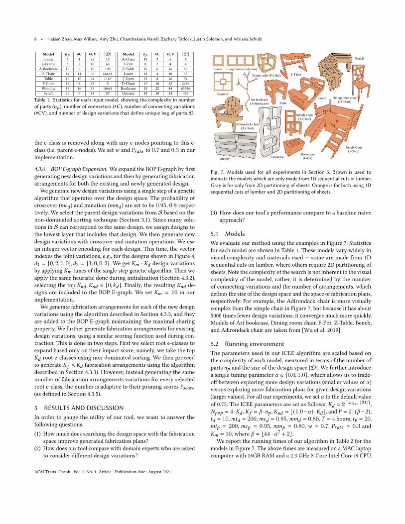
Model 𝑛𝑝 #C #CV |D | Model 𝑛𝑝 #C #CV |D |Frame 4 4 22 13 A-Chair 18 3 6 4L-Frame 6 8 16 65 F-Pot 8 1 4 4

A-Bookcase 12 6 16 192 Z-Table 15 6 16 63S-Chair 14 14 32 66438 Loom 18 4 10 36Table 12 10 24 1140 J-Gym 23 8 16 54F-Cube 12 8 23 5 D-Chair 17 10 22 2280Window 12 16 32 10463 Bookcase 15 22 44 65536Bench 29 6 14 57 Dresser 10 10 25 480

Table 1. Statistics for each input model, showing the complexity in numberof parts (𝑛𝑝 ), number of connectors (#C), number of connecting variations(#CV), and number of design variations that define unique bag of parts D.

the e-class is removed along with any e-nodes pointing to this e-class (i.e. parent e-nodes). We set𝑤 and 𝑃𝑟𝑎𝑡𝑒 to 0.7 and 0.3 in ourimplementation.

4.3.6 BOP E-graph Expansion. We expand the BOP E-graph by firstgenerating new design variations and then by generating fabricationarrangements for both the existing and newly generated design.

We generate new design variations using a single step of a geneticalgorithm that operates over the design space. The probability ofcrossover (𝑚𝑐𝑑 ) and mutation (𝑚𝑚𝑑 ) are set to be 0.95, 0.8 respec-tively. We select the parent design variations from S based on thenon-dominated sorting technique (Section 3.1). Since many solu-tions in S can correspond to the same design, we assign designs tothe lowest layer that includes that design. We then generate newdesign variations with crossover and mutation operations. We usean integer vector encoding for each design. This time, the vectorindexes the joint variations, e.g., for the designs shown in Figure 4,𝑑1 = [0, 2, 1, 0], 𝑑2 = [1, 0, 0, 2]. We get 𝐾𝑚 · 𝐾𝑑 design variationsby applying 𝐾𝑚 times of the single step genetic algorithm. Then weapply the same heuristic done during initialization (Section 4.3.2),selecting the top 𝐾𝑛𝑑 , 𝐾𝑛𝑑 ∈ [0, 𝑘𝑑 ]. Finally, the resulting 𝐾𝑛𝑑 de-signs are included to the BOP E-graph. We set 𝐾𝑚 = 10 in ourimplementation.

We generate fabrication arrangements for each of the new designvariations using the algorithm described in Section 4.3.3, and theyare added to the BOP E-graph maintaining the maximal sharingproperty. We further generate fabrication arrangements for existingdesign variations, using a similar scoring function used during con-traction. This is done in two steps. First we select root e-classes toexpand based only on their impact score; namely, we take the top𝐾𝑑 root e-classes using non-dominated sorting. We then proceedto generate 𝐾𝑓 × 𝐾𝑑 fabrication arrangements using the algorithmdescribed in Section 4.3.3). However, instead generating the samenumber of fabrication arrangements variations for every selectedroot e-class, the number is adaptive to their pruning scores 𝑃𝑠𝑐𝑜𝑟𝑒(as defined in Section 4.3.5).

5 RESULTS AND DISCUSSIONIn order to gauge the utility of our tool, we want to answer thefollowing questions:(1) How much does searching the design space with the fabrication

space improve generated fabrication plans?(2) How does our tool compare with domain experts who are asked

to consider different design variations?

Table

Frame Long Frame (L-Frame)

Window

Adirondack chair

(A-Chair)

Frame cube (F-Cube) Z-Table

Bench

Loom Dining room chair

(D-Chair)Art bookcase

(A-Bookcase)

Flower pot

(F-Pot)

Jungle Gym

(J-Gym)

Simple chair

(S-Chair)

BookcaseDresser

Fig. 7. Models used for all experiments in Section 5. Brown is used toindicate the models which are only made from 1D sequential cuts of lumber.Gray is for only from 2D partitioning of sheets. Orange is for both using 1Dsequential cuts of lumber and 2D partitioning of sheets.

(3) How does our tool’s performance compare to a baseline naïveapproach?

5.1 ModelsWe evaluate our method using the examples in Figure 7. Statisticsfor each model are shown in Table 1. These models vary widely invisual complexity and materials used — some are made from 1Dsequential cuts on lumber, where others require 2D partitioning ofsheets. Note the complexity of the search is not inherent to the visualcomplexity of the model, rather, it is determined by the numberof connecting variations and the number of arrangements, whichdefines the size of the design space and the space of fabrication plans,respectively. For example, the Adirondack chair is more visuallycomplex than the simple chair in Figure 7, but because it has about5000 times fewer design variations, it converges much more quickly.Models of Art bookcase, Dining room chair, F-Pot, Z-Table, Bench,and Adirondack chair are taken from [Wu et al. 2019].

5.2 Running environmentThe parameters used in our ICEE algorithm are scaled based onthe complexity of each model, measured in terms of the number ofparts 𝑛𝑝 and the size of the design space |D|. We further introducea single tuning parameter 𝛼 ∈ [0.0, 1.0], which allows us to trade-off between exploring more design variations (smaller values of 𝛼)versus exploring more fabrication plans for given design variations(larger values). For all our experiments, we set 𝛼 to the default valueof 0.75. The ICEE parameters are set as follows: 𝐾𝑑 = 2 ⌈log10 |D |⌉ ,𝑁𝑝𝑜𝑝 = 4 ·𝐾𝑑 ,𝐾𝑓 = 𝛽 ·𝑛𝑝 ,𝐾𝑛𝑑 = ⌊(1.0−𝛼) ·𝐾𝑑 ⌋, and 𝑃 = 2 · (𝛽−2),𝑡𝑑 = 10,𝑚𝑡𝑑 = 200,𝑚𝑐𝑑 = 0.95,𝑚𝑚𝑑 = 0.80,𝑇 = 4 hours, 𝑡𝑝 = 20,𝑚𝑡𝑝 = 200, 𝑚𝑐𝑝 = 0.95, 𝑚𝑚𝑝 = 0.80, 𝑤 = 0.7, 𝑃𝑟𝑎𝑡𝑒 = 0.3 and𝐾𝑚 = 10, where 𝛽 = ⌊44 · 𝛼7 + 2⌋.

We report the running times of our algorithm in Table 2 for themodels in Figure 7. The above times are measured on a MAC laptopcomputer with 16GB RAM and a 2.3 GHz 8-Core Intel Core i9 CPU.



More discussion of the running time is in the supplemental material.

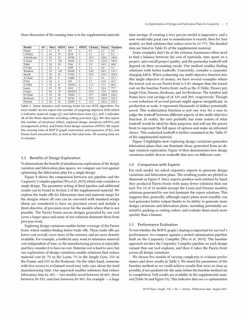
Model #O #Iter #EDV #Arr #PDV CEt(m) Et(m) Total(m)Frame 2 11 8 181 3 0.7 2.1 2.8L-Frame 2 24 19 2818 3 2.1 6.1 8.2A-Bookcase 3 25 25 28700 3 20.5 228.6 249.0S-Chair 2 15 136 35656 6 27.6 122.0 149.6Table 2 18 50 9346 9 5.9 34.9 40.8F-Cube 2 23 4 3499 3 1.4 4.0 5.5Window 2 23 116 81026 4 32.8 98.9 131.7Bench 2 25 16 37436 3 30.3 215.1 245.4A-Chair 2 28 4 14440 3 3.1 9.6 12.7F-Pot 3 14 3 185 2 1.7 13.0 14.7Z-Table 3 70 41 336091 6 17.1 71.1 88.2Loom 3 21 10 1812 5 3.1 74.6 77.7J-Gym 3 46 18 286239 3 37.0 72.0 109.0D-Chair 2 18 40 15054 7 27.7 228.8 256.5Bookcase 3 15 32 34756 11 39.4 336.8 376.3Dresser 3 20 44 22209 5 14.1 241.2 255.4

Table 2. Some statistics and running times for our ICEE algorithm. Foreach model, we firs report the number of targeting objective (#O) where2 indicates material usage (𝑓𝑐 ) and fabrication time (𝑓𝑡 ), and 3 indicatesall of the three objective including cutting precision (𝑓𝑝 ). We also reportthe number of iterations (#Iter), explored design variations (#EDV) andarrangements (#Arr), and Pareto front design variations (#PDV). We reportthe running time of BOP E-graph contraction and expansion (CEt), andPareto front extraction (Et), as well as the total time. All running time arein minutes.

5.3 Benefits of Design ExplorationTo demonstrate the benefit of simultaneous exploration of the designvariation and fabrication plan spaces, we compare our tool againstoptimizing the fabrication plan for a single design.Figure 8 shows the comparison between our pipeline and the

Carpentry Compiler pipeline [Wu et al. 2019] which only considers asingle design. The parameter setting of their pipeline and additionalresults can be found in Section 2 of the supplemental material. Weexplore the trade-offs for fabrication time and material usage forthe designs where all cuts can be executed with standard setups(these are considered to have no precision error) and include athird objective of precision error for the models where that is notpossible. The Pareto fronts across designs generated by our toolcover a larger space and many of our solutions dominate those fromprevious work.

Exploring design variations enables better coverage of the Paretofront, which enables finding better trade-offs. These trade-offs arelower-cost overall, cover more of the extrema, and are more denselyavailable. For example, a hobbyist may want to minimize materialcost independent of time, as the manufacturing process is enjoyable,and they consider it to have no cost. Material cost is hard to save, butour exploration of design variations enable solutions that reducematerial cost by 7% in the Loom, 7% in the Jungle Gym, 15% inthe Frame, and 25% in the Bookcase. On the other hand, someonewith free access to reclaimed wood may only care about the totalmanufacturing time. Our approach enables solutions that reducefabrication time by 60% — two models saved between 50-60%, threebetween 30-35%, and four between 20-30%, for example — a huge

time savings. If creating a very precise model is imperative, and auser would take great care to manufacture it exactly, then for fourmodels, we find solutions that reduce error by 61-77%. The detaileddata are listed in Table S5 of the supplemental material.Some examples don’t lie at the extrema: businesses often need

to find a balance between the cost of materials, time spent on aproject, and overall project quality, and the particular tradeoff willdepend on their accounting needs. Our method enables findingsolutions with better tradeoffs. Concretely, consider a carpentercharging $40/h. When scalarizing our multi-objective function intothis single objective of money, we have several examples wherethe lowest cost on our Pareto front is 5-8% cheaper than the lowestcost on the baseline Pareto front, such as the Z-Table, Flower pot,Jungle Gym, Dresser, Bookcase, and Art Bookcase. The window andframe have cost savings of of 12% and 20%, respectively. Thougha cost reduction of several percent might appear insignificant, inproduction at scale, it represents thousands of dollars potentiallysaved. This scalarization function is just one way for a user tojudge the tradeoff between different aspects of the multi-objectivefunction. In reality, the user probably has some notion of whattradeoff would be ideal for their purposes, and will use the paretofront to represent the full space of options and make an informedchoice. This scalarized tradeoff is further examined in the Table S7of the supplemental material.Figure 9 highlights how exploring design variations generates

fabrication plans that can dominate those generated from no de-sign variation exploration. Figure 10 then demonstrates how designvariations enable diverse tradeoffs that save on different costs.

5.4 Comparison with ExpertsFor each model, we asked carpentry experts to generate designvariations and fabrication plans. The resulting points are plotted asdiamonds in Figure 8. Since experts produce each solution by hand,they produced Pareto fronts with many fewer solutions than ourtool. For 14 of 16 models (except the Loom and Dresser models),solutions generated by our tool dominate the expert solutions. Thissuggests that, generally, although expert plans seem sensible, ourtool generates better output thanks to its ability to generate moredesign variations and fabrication plans, including potentially un-intuitive packing or cutting orders, and evaluate them much morequickly than a human.

5.5 Performance EvaluationTo test whether the BOP E-graph’s sharing is important for our tool’sperformance, we compare against a nested-optimization pipelinebuilt on the Carpentry Compiler [Wu et al. 2019]. The baselineapproach invokes the Carpentry Compiler pipeline on each designvariant that our tool explores, and then it takes the Pareto frontacross all design variations.

We choose five models of varying complexity to evaluate perfor-mance and show results in Table 3. We tuned the parameters of thebaseline method so we could achieve results that were as close aspossible, if not qualitatively the same (when the baseline method ranto completion). Full results are available in the supplemental mate-rial (Table S6 and Figure S1). This indicates that our co-optimization



No design exploration Expert resultsPareto fronts of our method

Pareto fronts of explored designs of our method

A-Bookcase

J-Gym Bookcase

Dresser

A-ChairWindowTableFrame

B

A

B

A

A

B

A

B

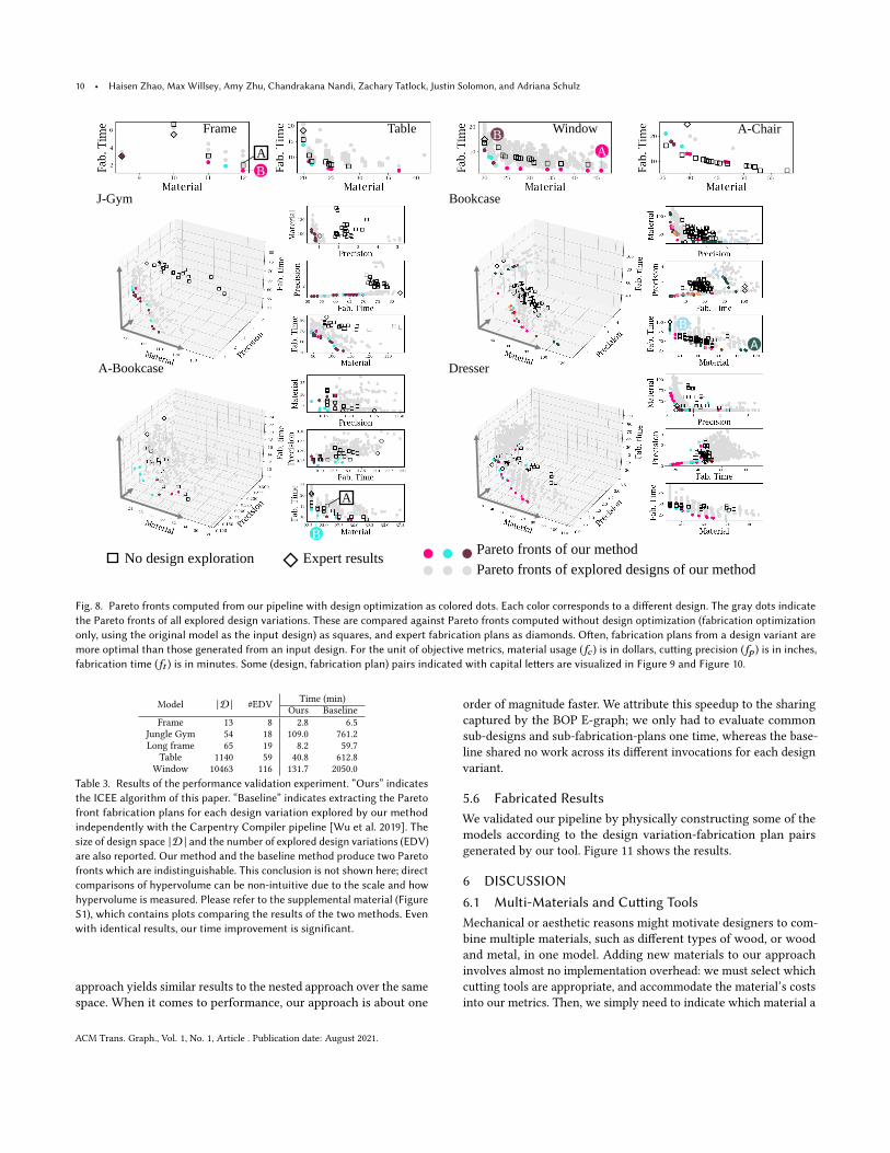
Fig. 8. Pareto fronts computed from our pipeline with design optimization as colored dots. Each color corresponds to a different design. The gray dots indicatethe Pareto fronts of all explored design variations. These are compared against Pareto fronts computed without design optimization (fabrication optimizationonly, using the original model as the input design) as squares, and expert fabrication plans as diamonds. Often, fabrication plans from a design variant aremore optimal than those generated from an input design. For the unit of objective metrics, material usage (𝑓𝑐 ) is in dollars, cutting precision (𝑓𝑝 ) is in inches,fabrication time (𝑓𝑡 ) is in minutes. Some (design, fabrication plan) pairs indicated with capital letters are visualized in Figure 9 and Figure 10.

Model |D | #EDV Time (min)Ours Baseline

Frame 13 8 2.8 6.5Jungle Gym 54 18 109.0 761.2Long frame 65 19 8.2 59.7

Table 1140 59 40.8 612.8Window 10463 116 131.7 2050.0

Table 3. Results of the performance validation experiment. “Ours” indicatesthe ICEE algorithm of this paper. “Baseline” indicates extracting the Paretofront fabrication plans for each design variation explored by our methodindependently with the Carpentry Compiler pipeline [Wu et al. 2019]. Thesize of design space |D | and the number of explored design variations (EDV)are also reported. Our method and the baseline method produce two Paretofronts which are indistinguishable. This conclusion is not shown here; directcomparisons of hypervolume can be non-intuitive due to the scale and howhypervolume is measured. Please refer to the supplemental material (FigureS1), which contains plots comparing the results of the two methods. Evenwith identical results, our time improvement is significant.

approach yields similar results to the nested approach over the samespace. When it comes to performance, our approach is about one

order of magnitude faster. We attribute this speedup to the sharingcaptured by the BOP E-graph; we only had to evaluate commonsub-designs and sub-fabrication-plans one time, whereas the base-line shared no work across its different invocations for each designvariant.

5.6 Fabricated ResultsWe validated our pipeline by physically constructing some of themodels according to the design variation-fabrication plan pairsgenerated by our tool. Figure 11 shows the results.

6 DISCUSSION

6.1 Multi-Materials and Cutting ToolsMechanical or aesthetic reasons might motivate designers to com-bine multiple materials, such as different types of wood, or woodand metal, in one model. Adding new materials to our approachinvolves almost no implementation overhead: we must select whichcutting tools are appropriate, and accommodate the material’s costsinto our metrics. Then, we simply need to indicate which material a



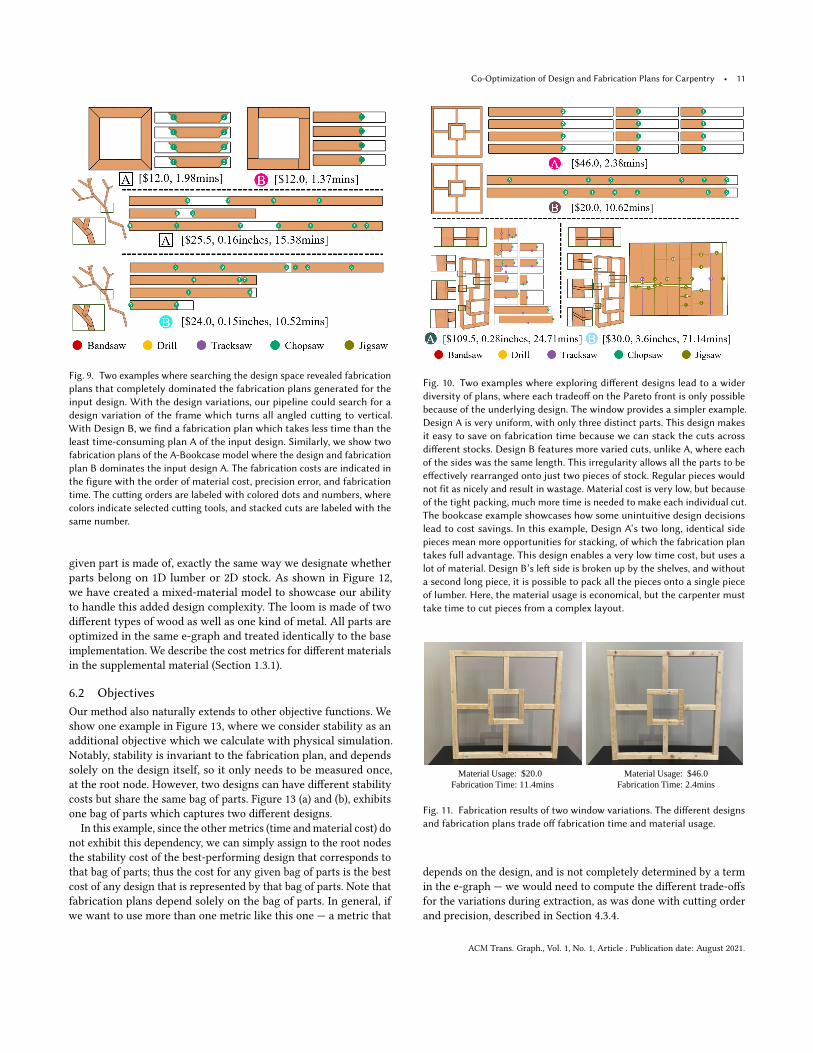
Fig. 9. Two examples where searching the design space revealed fabricationplans that completely dominated the fabrication plans generated for theinput design. With the design variations, our pipeline could search for adesign variation of the frame which turns all angled cutting to vertical.With Design B, we find a fabrication plan which takes less time than theleast time-consuming plan A of the input design. Similarly, we show twofabrication plans of the A-Bookcase model where the design and fabricationplan B dominates the input design A. The fabrication costs are indicated inthe figure with the order of material cost, precision error, and fabricationtime. The cutting orders are labeled with colored dots and numbers, wherecolors indicate selected cutting tools, and stacked cuts are labeled with thesame number.

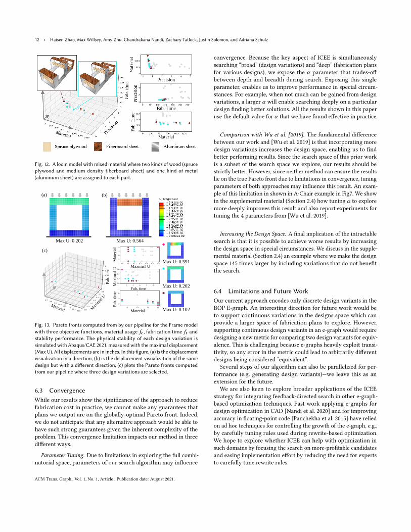
given part is made of, exactly the same way we designate whetherparts belong on 1D lumber or 2D stock. As shown in Figure 12,we have created a mixed-material model to showcase our abilityto handle this added design complexity. The loom is made of twodifferent types of wood as well as one kind of metal. All parts areoptimized in the same e-graph and treated identically to the baseimplementation. We describe the cost metrics for different materialsin the supplemental material (Section 1.3.1).

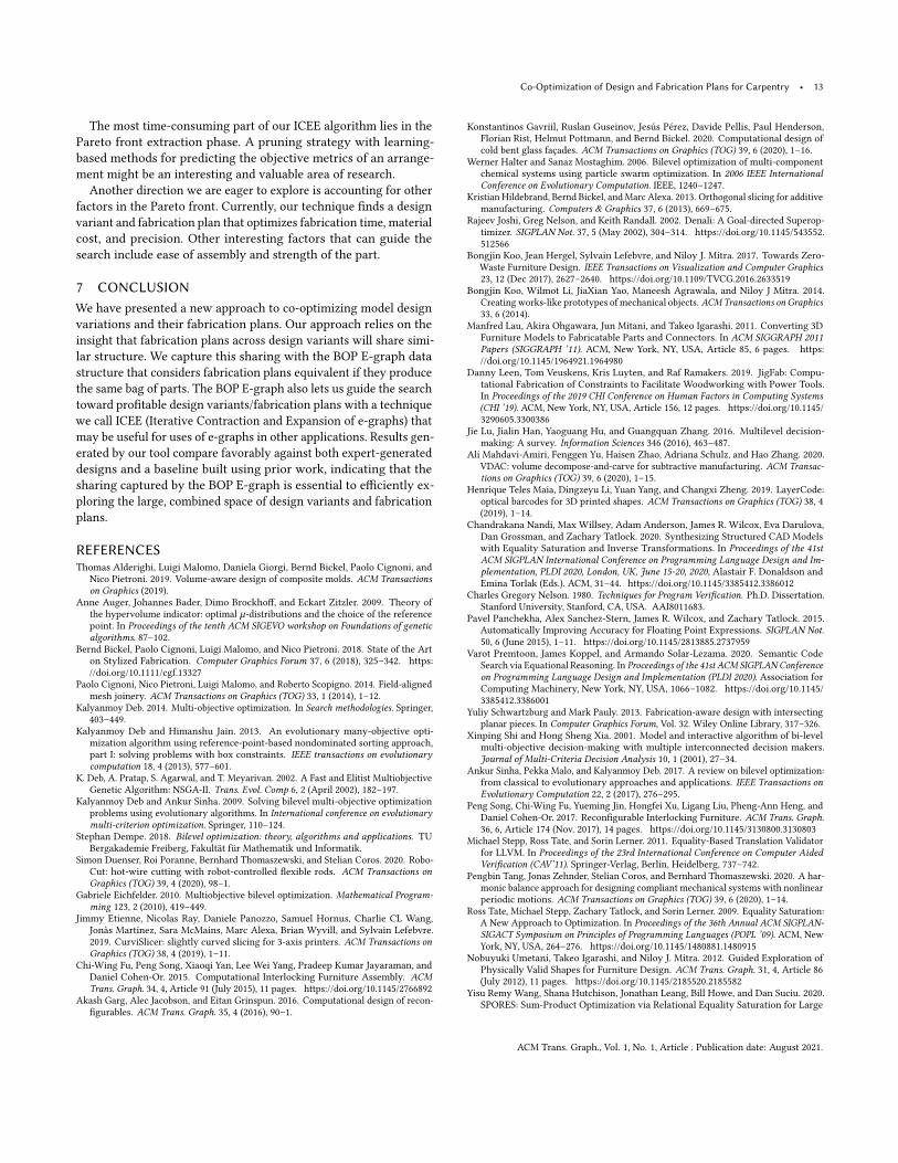
6.2 ObjectivesOur method also naturally extends to other objective functions. Weshow one example in Figure 13, where we consider stability as anadditional objective which we calculate with physical simulation.Notably, stability is invariant to the fabrication plan, and dependssolely on the design itself, so it only needs to be measured once,at the root node. However, two designs can have different stabilitycosts but share the same bag of parts. Figure 13 (a) and (b), exhibitsone bag of parts which captures two different designs.

In this example, since the other metrics (time andmaterial cost) donot exhibit this dependency, we can simply assign to the root nodesthe stability cost of the best-performing design that corresponds tothat bag of parts; thus the cost for any given bag of parts is the bestcost of any design that is represented by that bag of parts. Note thatfabrication plans depend solely on the bag of parts. In general, ifwe want to use more than one metric like this one — a metric that

Fig. 10. Two examples where exploring different designs lead to a widerdiversity of plans, where each tradeoff on the Pareto front is only possiblebecause of the underlying design. The window provides a simpler example.Design A is very uniform, with only three distinct parts. This design makesit easy to save on fabrication time because we can stack the cuts acrossdifferent stocks. Design B features more varied cuts, unlike A, where eachof the sides was the same length. This irregularity allows all the parts to beeffectively rearranged onto just two pieces of stock. Regular pieces wouldnot fit as nicely and result in wastage. Material cost is very low, but becauseof the tight packing, much more time is needed to make each individual cut.The bookcase example showcases how some unintuitive design decisionslead to cost savings. In this example, Design A’s two long, identical sidepieces mean more opportunities for stacking, of which the fabrication plantakes full advantage. This design enables a very low time cost, but uses alot of material. Design B’s left side is broken up by the shelves, and withouta second long piece, it is possible to pack all the pieces onto a single pieceof lumber. Here, the material usage is economical, but the carpenter musttake time to cut pieces from a complex layout.

Material Usage: $20.0

Fabrication Time: 11.4mins

Material Usage: $46.0

Fabrication Time: 2.4mins

Fig. 11. Fabrication results of two window variations. The different designsand fabrication plans trade off fabrication time and material usage.

depends on the design, and is not completely determined by a termin the e-graph — we would need to compute the different trade-offsfor the variations during extraction, as was done with cutting orderand precision, described in Section 4.3.4.



Fig. 12. A loommodel with mixed material where two kinds of wood (spruceplywood and medium density fiberboard sheet) and one kind of metal(aluminum sheet) are assigned to each part.

Max U: 0.202 Max U: 0.564

(a) (b)

(c)

Max U: 0.591

Max U: 0.202

Max U: 0.102

Maximal U

Max

imal

UF

ab.

tim

e

Fab. time

Mat

eria

l

Fab

. ti

me

Material

Fig. 13. Pareto fronts computed from by our pipeline for the Frame modelwith three objective functions, material usage 𝑓𝑐 , fabrication time 𝑓𝑡 andstability performance. The physical stability of each design variation issimulated with Abaqus/CAE 2021, measured with the maximal displacement(MaxU). All displacements are in inches. In this figure, (a) is the displacementvisualization in a direction, (b) is the displacement visualization of the samedesign but with a different direction, (c) plots the Pareto fronts computedfrom our pipeline where three design variations are selected.

6.3 ConvergenceWhile our results show the significance of the approach to reducefabrication cost in practice, we cannot make any guarantees thatplans we output are on the globally-optimal Pareto front. Indeed,we do not anticipate that any alternative approach would be able tohave such strong guarantees given the inherent complexity of theproblem. This convergence limitation impacts our method in threedifferent ways.

Parameter Tuning. Due to limitations in exploring the full combi-natorial space, parameters of our search algorithm may influence

convergence. Because the key aspect of ICEE is simultaneouslysearching “broad” (design variations) and “deep” (fabrication plansfor various designs), we expose the 𝛼 parameter that trades-offbetween depth and breadth during search. Exposing this singleparameter, enables us to improve performance in special circum-stances. For example, when not much can be gained from designvariations, a larger 𝛼 will enable searching deeply on a particulardesign finding better solutions. All the results shown in this paperuse the default value for 𝛼 that we have found effective in practice.

Comparison with Wu et al. [2019]. The fundamental differencebetween our work and [Wu et al. 2019] is that incorporating moredesign variations increases the design space, enabling us to findbetter performing results. Since the search space of this prior workis a subset of the search space we explore, our results should bestrictly better. However, since neither method can ensure the resultslie on the true Pareto front due to limitations in convergence, tuningparameters of both approaches may influence this result. An exam-ple of this limitation in shown in A-Chair example in Fig7. We showin the supplemental material (Section 2.4) how tuning 𝛼 to exploremore deeply improves this result and also report experiments fortuning the 4 parameters from [Wu et al. 2019].

Increasing the Design Space. A final implication of the intractablesearch is that it is possible to achieve worse results by increasingthe design space in special circumstances. We discuss in the supple-mental material (Section 2.4) an example where we make the designspace 145 times larger by including variations that do not benefitthe search.

6.4 Limitations and Future WorkOur current approach encodes only discrete design variants in theBOP E-graph. An interesting direction for future work would beto support continuous variations in the designs space which canprovide a larger space of fabrication plans to explore. However,supporting continuous design variants in an e-graph would requiredesigning a newmetric for comparing two design variants for equiv-alence. This is challenging because e-graphs heavily exploit transi-tivity, so any error in the metric could lead to arbitrarily differentdesigns being considered “equivalent”.Several steps of our algorithm can also be parallelized for per-

formance (e.g. generating design variants)—we leave this as anextension for the future.We are also keen to explore broader applications of the ICEE

strategy for integrating feedback-directed search in other e-graph-based optimization techniques. Past work applying e-graphs fordesign optimization in CAD [Nandi et al. 2020] and for improvingaccuracy in floating-point code [Panchekha et al. 2015] have reliedon ad hoc techniques for controlling the growth of the e-graph, e.g.,by carefully tuning rules used during rewrite-based optimization.We hope to explore whether ICEE can help with optimization insuch domains by focusing the search on more-profitable candidatesand easing implementation effort by reducing the need for expertsto carefully tune rewrite rules.



The most time-consuming part of our ICEE algorithm lies in thePareto front extraction phase. A pruning strategy with learning-based methods for predicting the objective metrics of an arrange-ment might be an interesting and valuable area of research.

Another direction we are eager to explore is accounting for otherfactors in the Pareto front. Currently, our technique finds a designvariant and fabrication plan that optimizes fabrication time, materialcost, and precision. Other interesting factors that can guide thesearch include ease of assembly and strength of the part.

7 CONCLUSIONWe have presented a new approach to co-optimizing model designvariations and their fabrication plans. Our approach relies on theinsight that fabrication plans across design variants will share simi-lar structure. We capture this sharing with the BOP E-graph datastructure that considers fabrication plans equivalent if they producethe same bag of parts. The BOP E-graph also lets us guide the searchtoward profitable design variants/fabrication plans with a techniquewe call ICEE (Iterative Contraction and Expansion of e-graphs) thatmay be useful for uses of e-graphs in other applications. Results gen-erated by our tool compare favorably against both expert-generateddesigns and a baseline built using prior work, indicating that thesharing captured by the BOP E-graph is essential to efficiently ex-ploring the large, combined space of design variants and fabricationplans.

REFERENCESThomas Alderighi, Luigi Malomo, Daniela Giorgi, Bernd Bickel, Paolo Cignoni, and

Nico Pietroni. 2019. Volume-aware design of composite molds. ACM Transactionson Graphics (2019).

Anne Auger, Johannes Bader, Dimo Brockhoff, and Eckart Zitzler. 2009. Theory ofthe hypervolume indicator: optimal `-distributions and the choice of the referencepoint. In Proceedings of the tenth ACM SIGEVO workshop on Foundations of geneticalgorithms. 87–102.

Bernd Bickel, Paolo Cignoni, Luigi Malomo, and Nico Pietroni. 2018. State of the Arton Stylized Fabrication. Computer Graphics Forum 37, 6 (2018), 325–342. https://doi.org/10.1111/cgf.13327

Paolo Cignoni, Nico Pietroni, Luigi Malomo, and Roberto Scopigno. 2014. Field-alignedmesh joinery. ACM Transactions on Graphics (TOG) 33, 1 (2014), 1–12.

Kalyanmoy Deb. 2014. Multi-objective optimization. In Search methodologies. Springer,403–449.

Kalyanmoy Deb and Himanshu Jain. 2013. An evolutionary many-objective opti-mization algorithm using reference-point-based nondominated sorting approach,part I: solving problems with box constraints. IEEE transactions on evolutionarycomputation 18, 4 (2013), 577–601.

K. Deb, A. Pratap, S. Agarwal, and T. Meyarivan. 2002. A Fast and Elitist MultiobjectiveGenetic Algorithm: NSGA-II. Trans. Evol. Comp 6, 2 (April 2002), 182–197.

Kalyanmoy Deb and Ankur Sinha. 2009. Solving bilevel multi-objective optimizationproblems using evolutionary algorithms. In International conference on evolutionarymulti-criterion optimization. Springer, 110–124.

Stephan Dempe. 2018. Bilevel optimization: theory, algorithms and applications. TUBergakademie Freiberg, Fakultät für Mathematik und Informatik.

Simon Duenser, Roi Poranne, Bernhard Thomaszewski, and Stelian Coros. 2020. Robo-Cut: hot-wire cutting with robot-controlled flexible rods. ACM Transactions onGraphics (TOG) 39, 4 (2020), 98–1.

Gabriele Eichfelder. 2010. Multiobjective bilevel optimization. Mathematical Program-ming 123, 2 (2010), 419–449.

Jimmy Etienne, Nicolas Ray, Daniele Panozzo, Samuel Hornus, Charlie CL Wang,Jonàs Martínez, Sara McMains, Marc Alexa, Brian Wyvill, and Sylvain Lefebvre.2019. CurviSlicer: slightly curved slicing for 3-axis printers. ACM Transactions onGraphics (TOG) 38, 4 (2019), 1–11.

Chi-Wing Fu, Peng Song, Xiaoqi Yan, Lee Wei Yang, Pradeep Kumar Jayaraman, andDaniel Cohen-Or. 2015. Computational Interlocking Furniture Assembly. ACMTrans. Graph. 34, 4, Article 91 (July 2015), 11 pages. https://doi.org/10.1145/2766892

Akash Garg, Alec Jacobson, and Eitan Grinspun. 2016. Computational design of recon-figurables. ACM Trans. Graph. 35, 4 (2016), 90–1.

Konstantinos Gavriil, Ruslan Guseinov, Jesús Pérez, Davide Pellis, Paul Henderson,Florian Rist, Helmut Pottmann, and Bernd Bickel. 2020. Computational design ofcold bent glass façades. ACM Transactions on Graphics (TOG) 39, 6 (2020), 1–16.

Werner Halter and Sanaz Mostaghim. 2006. Bilevel optimization of multi-componentchemical systems using particle swarm optimization. In 2006 IEEE InternationalConference on Evolutionary Computation. IEEE, 1240–1247.

Kristian Hildebrand, Bernd Bickel, andMarc Alexa. 2013. Orthogonal slicing for additivemanufacturing. Computers & Graphics 37, 6 (2013), 669–675.

Rajeev Joshi, Greg Nelson, and Keith Randall. 2002. Denali: A Goal-directed Superop-timizer. SIGPLAN Not. 37, 5 (May 2002), 304–314. https://doi.org/10.1145/543552.512566

Bongjin Koo, Jean Hergel, Sylvain Lefebvre, and Niloy J. Mitra. 2017. Towards Zero-Waste Furniture Design. IEEE Transactions on Visualization and Computer Graphics23, 12 (Dec 2017), 2627–2640. https://doi.org/10.1109/TVCG.2016.2633519

Bongjin Koo, Wilmot Li, JiaXian Yao, Maneesh Agrawala, and Niloy J Mitra. 2014.Creating works-like prototypes of mechanical objects. ACMTransactions on Graphics33, 6 (2014).

Manfred Lau, Akira Ohgawara, Jun Mitani, and Takeo Igarashi. 2011. Converting 3DFurniture Models to Fabricatable Parts and Connectors. In ACM SIGGRAPH 2011Papers (SIGGRAPH ’11). ACM, New York, NY, USA, Article 85, 6 pages. https://doi.org/10.1145/1964921.1964980

Danny Leen, Tom Veuskens, Kris Luyten, and Raf Ramakers. 2019. JigFab: Compu-tational Fabrication of Constraints to Facilitate Woodworking with Power Tools.In Proceedings of the 2019 CHI Conference on Human Factors in Computing Systems(CHI ’19). ACM, New York, NY, USA, Article 156, 12 pages. https://doi.org/10.1145/3290605.3300386

Jie Lu, Jialin Han, Yaoguang Hu, and Guangquan Zhang. 2016. Multilevel decision-making: A survey. Information Sciences 346 (2016), 463–487.

Ali Mahdavi-Amiri, Fenggen Yu, Haisen Zhao, Adriana Schulz, and Hao Zhang. 2020.VDAC: volume decompose-and-carve for subtractive manufacturing. ACM Transac-tions on Graphics (TOG) 39, 6 (2020), 1–15.

Henrique Teles Maia, Dingzeyu Li, Yuan Yang, and Changxi Zheng. 2019. LayerCode:optical barcodes for 3D printed shapes. ACM Transactions on Graphics (TOG) 38, 4(2019), 1–14.

Chandrakana Nandi, Max Willsey, Adam Anderson, James R. Wilcox, Eva Darulova,Dan Grossman, and Zachary Tatlock. 2020. Synthesizing Structured CAD Modelswith Equality Saturation and Inverse Transformations. In Proceedings of the 41stACM SIGPLAN International Conference on Programming Language Design and Im-plementation, PLDI 2020, London, UK, June 15-20, 2020, Alastair F. Donaldson andEmina Torlak (Eds.). ACM, 31–44. https://doi.org/10.1145/3385412.3386012

Charles Gregory Nelson. 1980. Techniques for Program Verification. Ph.D. Dissertation.Stanford University, Stanford, CA, USA. AAI8011683.

Pavel Panchekha, Alex Sanchez-Stern, James R. Wilcox, and Zachary Tatlock. 2015.Automatically Improving Accuracy for Floating Point Expressions. SIGPLAN Not.50, 6 (June 2015), 1–11. https://doi.org/10.1145/2813885.2737959

Varot Premtoon, James Koppel, and Armando Solar-Lezama. 2020. Semantic CodeSearch via Equational Reasoning. In Proceedings of the 41st ACM SIGPLAN Conferenceon Programming Language Design and Implementation (PLDI 2020). Association forComputing Machinery, New York, NY, USA, 1066–1082. https://doi.org/10.1145/3385412.3386001

Yuliy Schwartzburg and Mark Pauly. 2013. Fabrication-aware design with intersectingplanar pieces. In Computer Graphics Forum, Vol. 32. Wiley Online Library, 317–326.

Xinping Shi and Hong Sheng Xia. 2001. Model and interactive algorithm of bi-levelmulti-objective decision-making with multiple interconnected decision makers.Journal of Multi-Criteria Decision Analysis 10, 1 (2001), 27–34.

Ankur Sinha, Pekka Malo, and Kalyanmoy Deb. 2017. A review on bilevel optimization:from classical to evolutionary approaches and applications. IEEE Transactions onEvolutionary Computation 22, 2 (2017), 276–295.

Peng Song, Chi-Wing Fu, Yueming Jin, Hongfei Xu, Ligang Liu, Pheng-Ann Heng, andDaniel Cohen-Or. 2017. Reconfigurable Interlocking Furniture. ACM Trans. Graph.36, 6, Article 174 (Nov. 2017), 14 pages. https://doi.org/10.1145/3130800.3130803

Michael Stepp, Ross Tate, and Sorin Lerner. 2011. Equality-Based Translation Validatorfor LLVM. In Proceedings of the 23rd International Conference on Computer AidedVerification (CAV’11). Springer-Verlag, Berlin, Heidelberg, 737–742.

Pengbin Tang, Jonas Zehnder, Stelian Coros, and Bernhard Thomaszewski. 2020. A har-monic balance approach for designing compliant mechanical systems with nonlinearperiodic motions. ACM Transactions on Graphics (TOG) 39, 6 (2020), 1–14.

Ross Tate, Michael Stepp, Zachary Tatlock, and Sorin Lerner. 2009. Equality Saturation:A New Approach to Optimization. In Proceedings of the 36th Annual ACM SIGPLAN-SIGACT Symposium on Principles of Programming Languages (POPL ’09). ACM, NewYork, NY, USA, 264–276. https://doi.org/10.1145/1480881.1480915

Nobuyuki Umetani, Takeo Igarashi, and Niloy J. Mitra. 2012. Guided Exploration ofPhysically Valid Shapes for Furniture Design. ACM Trans. Graph. 31, 4, Article 86(July 2012), 11 pages. https://doi.org/10.1145/2185520.2185582

Yisu Remy Wang, Shana Hutchison, Jonathan Leang, Bill Howe, and Dan Suciu. 2020.SPORES: Sum-Product Optimization via Relational Equality Saturation for Large


https://doi.org/10.1111/cgf.13327

https://doi.org/10.1111/cgf.13327

https://doi.org/10.1145/2766892

https://doi.org/10.1145/543552.512566

https://doi.org/10.1145/543552.512566

https://doi.org/10.1109/TVCG.2016.2633519

https://doi.org/10.1145/1964921.1964980

https://doi.org/10.1145/1964921.1964980

https://doi.org/10.1145/3290605.3300386

https://doi.org/10.1145/3290605.3300386

https://doi.org/10.1145/3385412.3386012

https://doi.org/10.1145/2813885.2737959

https://doi.org/10.1145/3385412.3386001

https://doi.org/10.1145/3385412.3386001

https://doi.org/10.1145/3130800.3130803

https://doi.org/10.1145/1480881.1480915

https://doi.org/10.1145/2185520.2185582


Scale Linear Algebra. Proc. VLDB Endow. 13, 12 (July 2020), 1919–1932. https://doi.org/10.14778/3407790.3407799

Ziqi Wang, Peng Song, Florin Isvoranu, and Mark Pauly. 2019. Design and structuraloptimization of topological interlocking assemblies. ACM Transactions on Graphics(TOG) 38, 6 (2019), 1–13.

Max Willsey, Chandrakana Nandi, Yisu Remy Wang, Oliver Flatt, Zachary Tatlock, andPavel Panchekha. 2021. egg: Fast and Extensible Equality Saturation. Proc. ACMProgram. Lang. 5, POPL, Article 23 (Jan. 2021), 29 pages. https://doi.org/10.1145/3434304

Chenming Wu, Haisen Zhao, Chandrakana Nandi, Jeffrey I Lipton, Zachary Tatlock,and Adriana Schulz. 2019. Carpentry compiler. ACM Transactions on Graphics (TOG)38, 6 (2019), 1–14.

Jinfan Yang, Chrystiano Araujo, Nicholas Vining, Zachary Ferguson, Enrique Rosales,Daniele Panozzo, Sylvain Lefevbre, Paolo Cignoni, and Alla Sheffer. 2020. DHFSlicer:

double height-field slicing for milling fixed-height materials. ACM Transactions onGraphics (TOG) 39, 6 (2020), 1–17.

Yong-Liang Yang, Jun Wang, and Niloy J Mitra. 2015. Reforming Shapes for Material-aware Fabrication. In Computer Graphics Forum, Vol. 34. Wiley Online Library,53–64.

Yafeng Yin. 2000. Genetic-algorithms-based approach for bilevel programming models.Journal of transportation engineering 126, 2 (2000), 115–120.

Xiaoting Zhang, Guoxin Fang, Mélina Skouras, Gwenda Gieseler, Charlie Wang, andEmily Whiting. 2019. Computational design of fabric formwork. (2019).

Haisen Zhao, Fanglin Gu, Qi-Xing Huang, Jorge Garcia, Yong Chen, Changhe Tu,Bedrich Benes, Hao Zhang, Daniel Cohen-Or, and Baoquan Chen. 2016. Connectedfermat spirals for layered fabrication. ACM Transactions on Graphics (TOG) 35, 4(2016), 1–10.


https://doi.org/10.14778/3407790.3407799

https://doi.org/10.14778/3407790.3407799

https://doi.org/10.1145/3434304

https://doi.org/10.1145/3434304

Documents

Co-Optimization of Design and Fabrication Plans for Carpentry