Co-Learning Patterns As Emergent Market Phenomena: An

IOWA STATE UNIVERSITY Department of Economics Ames, Iowa, 50011-‐1070

Iowa State University does not discriminate on the basis of race, color, age, religion, national origin, sexual orientation, gender identity, genetic information, sex, marital status, disability, or status as a U.S. veteran. Inquiries can be directed to the Director of Equal Opportunity and Compliance, 3280 Beardshear Hall, (515) 294-‐7612.

Co-Learning Patterns As Emergent MarketPhenomena: An Electricity Market Illustration

Hongyan Li, Leigh Tesfatsion

Working Paper No. 10042December 2010Revised on June 2011

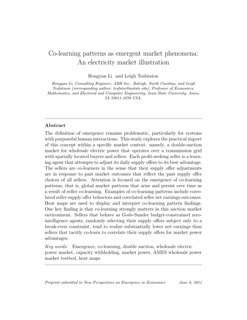
Co-learning patterns as emergent market phenomena:

An electricity market illustration

Hongyan Li and Leigh Tesfatsion

Hongyan Li, Consulting Engineer, ABB Inc., Raleigh, North Carolina, and LeighTesfatsion (corresponding author: [email protected]), Professor of Economics,

Mathematics, and Electrical and Computer Engineering, Iowa State University, Ames,IA 50011-1070 USA.

Abstract

The definition of emergence remains problematic, particularly for systemswith purposeful human interactions. This study explores the practical importof this concept within a specific market context: namely, a double-auctionmarket for wholesale electric power that operates over a transmission gridwith spatially located buyers and sellers. Each profit-seeking seller is a learn-ing agent that attempts to adjust its daily supply offers to its best advantage.The sellers are co-learners in the sense that their supply offer adjustmentsare in response to past market outcomes that reflect the past supply offerchoices of all sellers. Attention is focused on the emergence of co-learningpatterns, that is, global market patterns that arise and persist over time asa result of seller co-learning. Examples of co-learning patterns include corre-lated seller supply offer behaviors and correlated seller net earnings outcomes.Heat maps are used to display and interpret co-learning pattern findings.One key finding is that co-learning strongly matters in this auction marketenvironment. Sellers that behave as Gode-Sunder budget-constrained zero-intelligence agents, randomly selecting their supply offers subject only to abreak-even constraint, tend to realize substantially lower net earnings thansellers that tacitly co-learn to correlate their supply offers for market poweradvantages.

Key words: Emergence, co-learning, double auction, wholesale electricpower market, capacity withholding, market power, AMES wholesale powermarket testbed, heat maps

Preprint submitted to New Perspectives on Emergence in Economics June 8, 2011

1. Introduction

Emergence is an intriguing multi-faceted concept whose meaning remainscontroversial, particularly for systems involving purposeful human interac-tions. Consequently, it is of interest to study the practical import of thisconcept for economics by examining its role in specific realistically-renderedeconomic contexts.

This study examines emergence in an empirically-based model of a double-auction market for wholesale electric power. The market operates over a 5-bus transmission grid with spatially located buyers and sellers. Each profit-seeking seller is a learning agent that attempts to adjust its daily supply offersto its best advantage. The sellers are individual learners in the sense that thelearning method of each seller is calibrated (pre-tuned) to the attributes ofthe seller’s specific decision environment to capture learning-to-learn effects.However, the sellers are also co-learners in the sense that the adjustments oftheir daily supply offers are in response to past market outcomes that reflectthe past supply offer choices of all sellers.

Each seller in our model can engage in two forms of strategic capacitywithholding in an attempt to influence market prices to its own advantage,i.e., in an attempt to exercise market power . The seller can engage in eco-nomic capacity withholding (reporting supply offers with higher-than-truemarginal costs), and/or it can engage in physical capacity withholding (re-porting supply offers with lower-than-true maximum generation capacities).Economic and physical capacity withholding are the two main ways in whichreal-world energy sellers can exercise market power. Consequently, it is of in-terest to energy market operators, for market power mitigation purposes, tounderstand which form of market power affords greatest advantage to energysellers. Economic capacity withholding is relatively easy to monitor, to theextent that a seller’s fuel type gives a strong indication of its true marginalcosts. Strategic physical capacity withholding can be difficult to distinguishfrom outages and other events that cause unintentional reductions in avail-able generation capacity.

Systematic computational experiments are then conducted to explore theemergence of co-learning patterns , that is, global market patterns that ariseand persist over time as a result of seller co-learning. The specific co-learningpatterns of interest here are correlated seller supply offer behaviors and cor-related seller net earnings outcomes.

One key finding is that learning strongly matters in our double-auction

2

environment. Sellers that behave as Gode and Sunder (1993,1997) budget-constrained zero-intelligence agents, randomly selecting their supply offerssubject only to a break-even constraint, tend to realize substantially lowernet earnings than sellers that tacitly co-learn to correlate their supply of-fers for market power advantages. A second key finding is that learning-to-learn strongly matters. The co-learning sellers perform much better whenthe parameters of their learning methods are calibrated to sweet-spot valuesreflecting the attributes of their particular decision environment, includingboth own attributes (e.g., size, cost function, and location) and rival sellerattributes. A third key finding is that the pure exercise of economic capac-ity withholding is typically much more profitable for sellers than any use ofphysical capacity withholding.

A number of previous electricity researchers have separately explored ei-ther economic capacity withholding or physical capacity withholding exer-cised by learning traders, including the current authors. For example, Liand Tesfatsion (2009a) conduct preliminary learning experiments focusingon seller physical capacity withholding. Li, Sun, and Tesfatsion (2008,2009)explore the emergence of spatially correlated price patterns supported byseller co-learning when sellers can learn to exercise economic capacity with-holding. Li and Tesfatsion (2011) explore the effects of seller co-learning ontotal net surplus (efficiency) and the distribution of surplus among sellers,buyers, and the ISO when sellers can learn to exercise economic capacitywithholding.

The only previous work we are aware of that permits learning traders toengage simultaneously in both economic and physical capacity withholdingis Tellidou and Bakirtzis (2007). The latter authors analyze an electricitymarket operating over a 2-bus transmission grid in which seller supply of-fers take the form of an offered quantity and an offered price. The offeredquantity can be less than or equal to the seller’s true maximum generationcapacity, and the offered price can be greater than or equal to the seller’s truereservation price. However, the authors do not undertake any comparativeanalysis to determine the relative advantages to sellers of the two forms ofmarket power exercise. Moreover, all sellers are assumed to use the sameidentically parameterized learning method.

With regard to the general economics literature, it is rare to see physi-

3

cal capacity withholding treated at all.1 This could be due, in part, to theanalytical complications that arise when physical capacity withholding leadsto binding capacity constraints. It could also be due to the folk belief that,when it comes to the exercise of market power, economic and physical ca-pacity withholding are essentially equivalent means. When physical capacitywithholding is considered, it is typically within game contexts in which thefocus is on the existence of Nash equilibria without consideration of learningcapabilities [e.g., Dechenaux and Kovenock (2007)].

We begin our study in Section 2 with a summary discussion of emergenceas it has previously been defined and used for economic systems. A key con-clusion from this section is that the concept of weak emergence developedby Bedau (1997) is particularly relevant for the study of real-world economicsystems – such as electric power markets – whose complex interweaving ofphysical constraints, institutional rules, and strategic human behaviors ren-ders them analytically intractable. Roughly, Bedau defines a property P ofa system to be weakly emergent if P can be systematically generated for thesystem through a finite simulation, but through no other means.

Section 3 presents our wholesale electric power market model. This modelis implemented by means of the AMES Wholesale Power Market Testbed [Liand Tesfatsion (2009b,c), Tesfatsion (2010)], an agent-based computationallaboratory that incorporates institutional and structural features character-izing actual U.S. wholesale electric power markets. In keeping with actualpractice, AMES implements a two-settlement system consisting of a forwardday-ahead market and a real-time balancing market that operate over a high-voltage alternating current (HVAC) transmission grid. The day-ahead mar-ket is organized as a double auction in which wholesale buyers submit dailydemand bids to buy energy, wholesale sellers submit daily supply offers to sellenergy, and “locational marginal prices” are determined locally (for each hourat each grid bus) to maximize total net surplus subject to transmission andgeneration constraints. Traders in AMES can be modeled as learning agentswho adjust their demand bids and supply offers over time in an attempt toexercise market power.

In Section 4 we explain the experimental design used to test for the (weak)

1For example, firm behavior with potentially binding production capacity constraintsis only considered within one relatively small section (pp. 211-234) of the well-known 479-page industrial organization textbook by Tirole (2003) used in graduate and advancedundergraduate economics courses.

4

emergence of two types of co-learning patterns in our market model: namely,correlated seller supply offer behaviors, and correlated seller net earningsoutcomes. In particular, we develop a series of test cases for a 5-bus wholesaleelectric power market in which the exercise of seller market power takes one ofthree forms: economic capacity withholding; physical capacity withholding;or some combination of the two.

Section 5 explains steps taken prior to our test-case experimentation tocalibrate each seller’s learning parameters to sweet-spot values attuned toeach seller’s actual decision environment. For example, each seller’s initialaspiration level for net earnings is calibrated to its actual net earnings op-portunities as structurally determined by its feasible supply offers in relationto its true marginal cost function. Heat maps are used to display and inter-pret these sweet-spot patterns. A heat map is a two-dimensional graphicaldepiction of data in which groups of associated data values are distinguishedfrom one another by distinct colorings.

Sections 6-8 report our test-case experimental findings regarding the emer-gence of two types of co-learning patterns: correlated seller supply offer be-haviors, and correlated seller net earnings outcomes. Heat maps are usedto display and interpret these correlations. These heat map depictions canbe viewed as extensions of traditional industrial organization measures for(strategic) substitution and complementarity defined in terms of the signs of(cross) partial derivatives evaluated at a point in time [Bulow et al. (1985)].2

In the present context, which involves repeated stochastic choice by learningprofit-seeking traders embedded in an interaction network operating over aphysical network, more comprehensive ways are needed to measure the effectsof one trader’s actions on the actions and outcomes of other traders.

The key findings from the test-case experiments reported in Sections 6-8are summarized and compared in Section 9. Concluding remarks are given inSection 10. For improved expositional clarity, technical materials regardingseller cost and net earnings functions, seller learning methods, and sweet-spot learning parameter calibrations are gathered together in appendices tothis study.

2More precisely, a firm A’s product is said to be a substitute (or complement) for firm Bif more “aggressive” action by firm A, measured by an increase in some variable SA, resultsin a decrease (increase) in the profits πB of firm B. Strategic substitutes (complements)are defined in terms of the effects of a change in SA on the marginal profitability of firmB, that is, in terms of the sign of ∂2πB/∂SB∂SA.

5

2. Emergence in Economic Systems

This section briefly reviews how emergence has previously been definedand used for the study of economic systems.3 Of special interest are thecomplications caused by the presence of one or more agents with learningcapabilities.

Kuperberg (2006) provides an historical overview of emergence concep-tions in the economics literature. He begins in 1976 with the “invisible hand”of Adam Smith (1937). He then proceeds to a discussion of the “micromo-tives of macrobehavior” ideas of Schelling (1978) and the work of modern-dayeconomists such as Alan Kirman (1993) espousing “a new kind of economics”now known as agent-based computational economics [Tesfatsion and Judd(2006)].4 Kuperberg concludes there is no universally agreed upon definitionof emergence, yet three core characteristics can be identified. First, theremust be at least two distinct levels of organization. Second, at the lowerlevel of organization, a multitude of individual agents operate in accordancewith rules. Third, aggregate outcomes occur at the higher level of organiza-tion that result from the interactions of these individual agents but that arenot easily derivable from the rules followed by the individual agents.

Harper and Endres (2010) focus on conceptions of emergence in the mod-ern economics literature. They conclude (page 3) that this literature reveals“an incomplete patchwork of fragmented and contradictory notions of emer-gence.” Table 1 (page 6) of their study homes in on differences in usage be-tween evolutionary-institutional economists and complexity economists whoview economies as dynamic systems of interacting components (agents, units,entities, ...). Each specific usage captures a potentially important facet ofmessy economic reality: for example, novelty, non-reducibility of wholes totheir parts, downward causation, self-organization (bottom-up growth), re-currence of regular patterns, and unpredictability.

3Detailed discussions examining historical and current controversies surrounding theconcept of emergence as used in a variety of disciplines can be found in Anderson (1972),Auyang (1998), Stephan (1999), Corning (2002), O’Connor and Wong (2006), andDessalles et al. (2008). Discussions of emergence for general social science systems canbe found in Gilbert (1995), Hodgson (2000), and Squazzoni (2006).

4Somewhat surprisingly, Kuperberg makes no mention of Hayek (1948), whose recogni-tion that markets can be “spontaneously ordered” through the coordination capabilities ofprice mechanisms surely represents a relatively early identification of an emergent propertyfor economic systems [Lewis (2011)].

6

Referring to works by Stephan (1998) and Corning (2002), among oth-ers, Harper and Endres identify core features commonly seen in delineationsof emergence for economic systems which they suggest should be viewed asminimally necessary for emergence. Briefly, in order for a pattern, prop-erty, or relation to be emergent for an economic system, it must arise frommaterial components and depend upon the organization (connections andinteractions) of these components, not simply upon individual componentproperties. Harper and Endres then identify additional features particularlyrelevant to evolutionary economics which, together with the core features,constitute a stronger form of emergence: namely, genuine novelty; unpre-dictability in principle; and irreducibility to system component propertieseither in isolation or in other simpler systems.

What are the implications for emergence when one of more “constitutentparts” of a system are agents with learning capabilities? The general dis-cussions of potential downward causation (from macroscopic to microscopiclevels) appearing in some articles [e.g., Section 5 of Lewis (2011)] clearlyrelate to this issue. However, the issue is more directly addressed in theliterature surveyed by Dessalles et al. (2008) on emergence in multi-agentsystems. This literature explicitly recognizes that cognitive agents can beconstrained “by the whole” because perceived social phenomena can affecttheir behaviors and decisions. Dessalles et al. (2008) also provide their ownthoughtful discussion of implications for emergence when agents are cognitiveobservers of the world within which they interact and understand to variousextents their collective ability to affect social outcomes.5

As elaborated in Borrill and Tesfatsion (2011), real people combine con-structive and non-constructive aspects; they can only acquire new data aboutthe world constructively, through interactions, but they can have possibly un-computable beliefs about the world that influence their interactions. Thesebeliefs about the world can arise from inborn attributes, from communica-tions received from other agents, or from the use of non-constructive methods

5There is a strand of research not covered by Dessalles et al. (2008) that focuses on theemergence of social conventions in multi-agent systems with co-learning agents; see, forexample, Shoham and Tennenholtz (1994), Kittock (1995), Delgago (2002), and Urbano etal. (2009) However, the focus of this literature is on network topology: specifically, how dodifferent interaction networks (e.g., scale-free versus small-world networks) affect the speedwith which conventions emerge. The relationship between co-learning and emergence isnot specifically addressed.

7

(e.g., proof by contradiction) to interpret acquired data. To the extent thatthese beliefs involve perceptions of systemic properties, they provide a chan-nel through which systemic properties can act back upon microscopic states.Interestingly, agent-based modeling permits decision-making agents to belearners who form both constructive and non-constructive beliefs about theirvirtual computational world as guides for their interactions, and whose in-teractions in turn inform their beliefs. These powerful modeling capabilitiesshould greatly facilitate the study of emergence in real-world social systems.

In all of the emergence studies mentioned above, the focus is on the emer-gence of some pattern, property, or relation within a structurally given dy-namic system. As will be concretely demonstrated in the remaining sectionsof this study, emergence in dynamic systems can also usefully be studied ata higher level using structural perturbation methods.

Specifically, structural perturbation methods similar to those used tostudy chaotic processes and fractal systems [Devaney and Keen, 1989] canby used to generate an ensemble of possible dynamic system trajectories intrajectory space. By an appropriate coloring of these trajectories (or of theirpre-images in a parameter domain), interesting patterns can sometimes berevealed that provide a unique and informative “fingerprint” for the dynamicsystem.6

As a simple economic illustration, consider a discrete-time dynamic sys-tem that generates a unique net earnings level for each of N market tradersover time, starting from an exogenously given system state z1 in time period1. Suppose the system structure depends on a parameter α. The distributionof net earnings for the N traders at any given time t ≥ 1 would typically berepresented by some form of histogram that associates each possible net earn-ings level with a frequency of occurrence in the population. Alternatively,however, this distribution can be represented as a single point pt(z1, α) in anN -dimensional space, where each coordinate of pt(z1, α) gives the net earn-ings level of a particular trader in period t, conditional on z1 and α. One

6A famous example of this is the Mandelbrot set; see Branner (1998). The Mandelbrotset M is the set of all points c in the complex plane C for which the sequence (zt(c)) inC does not diverge to ∞ as t tends to ∞, where z1(c) = 0 and zt+1(c) = [zt(c)]2 + c fort ≥ 1. The intricately beautiful irregular regularity of M is revealed by (i) coloring blackall c-points lying in M , (ii) roughly partitioning the c-points in C lying outside M intofinitely many subsets in accordance with the differential divergence rates of zt(c), and (iii)using (non-black) colors to differentially visualize the c-points lying in these subsets.

8

can then consider the loci of points traced out by pt(z1, α) in N -space as α issystematically varied over a feasible range of α-values, or the trajectory (or-bit) traced out by pt(z1, α) in N -space as t is varied from 1 to ∞, or variousother tracings resulting from individual or combined changes in t, z1, and α.

In what sense do the patterns revealed by differential colorings of thesetracings represent emergent patterns? Here we make recourse to Bedau(1997) to argue that these patterns can be emergent in a weak sense fordynamic models attempting to capture the salient characteristics of compli-cated real-world systems.

The concept of weak emergence was introduced by Bedau (1997) in an at-tempt to obtain a well-defined, practical, and scientifically relevant definitionof emergence that sidesteps difficult philosophical and practical issues asso-ciated with definitions involving stronger requirements. Specifically, Bedaudefines a macrostate P of a system S with a microdynamic D, initial condi-tions C, and possibly additional external conditions E to be weakly emergentfor S if and only if P can be derived from {D,C,E}, but only by means ofa finite simulation.

Bedau further notes that this core concept of weak emergence, restrictedto a given system macrostate P, can be extended in a natural way to char-acterize the weak emergence of system patterns , i.e., collections of suitablyrelated system macrostates. As stressed by Laughlin et al. (2000) and Laugh-lin (2000), even when the underlying microscopic properties and relationshipsfor a dynamic system are not fully understood, the hope would be to findhigher-level organizational principles that reliably associate collections of re-lated microscopic states to collections of related macroscopic states, thusallowing some form of quantitative analysis to proceed.

Relating this back to earlier discussion, one way to visually differen-tiate among Bedau’s distinct system patterns would be through the useof distinct colorings for the collections of system macrostates constitutingthese patterns. Heat maps could then be obtained by projecting the coloredmacrostates into various two-dimensional subspaces of interest. These heatmaps could help to elucidate complex relationships between structural, in-stitutional, and behavioral conditions and the appearance and persistence ofsystem patterns. In the remaining sections of this study we illustrate howheat-maps can be used to visualize the weak emergence of system patternsfor the concrete case of a wholesale electric power market.

9

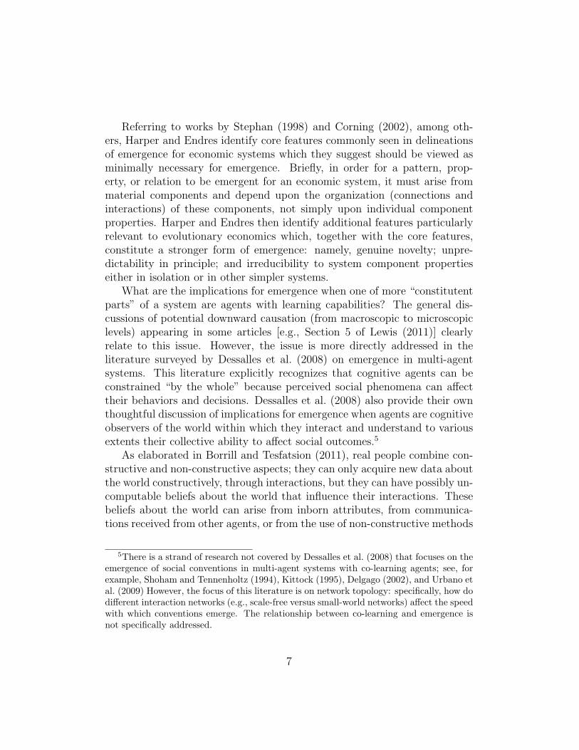
Figure 1: Key Features of the AMES Wholesale Power Market Testbed.

3. AMES Wholesale Power Market Testbed: Overview

The wholesale electric power market model used in this study is imple-mented using the AMES software platform. AMES (Agent-based M odelingof E lectricity Systems) is an open-source wholesale power market testbeddeveloped entirely in Java by researchers at Iowa State University. The lat-est version of AMES can be freely downloaded either at the AMES homepage[Tesfatsion (2010)] or through the IEEE Task Force on Open Source Software[IEEE (2011)].

This section describes the key features of Version 2.05 of AMES, used inthis study.7 These key features reflect, in simplified form, actual U.S. whole-sale electric power market operations in the Midwest (MISO), New England(ISO-NE), New York (NYISO), the mid-Atlantic states (PJM), California(CAISO), Texas (ERCOT), and the Southwest (SPP). A summary listing ofthese key features is provided in Fig. 1.

The AMES(V2.05) wholesale power market operates over a high-voltagealternating current (HVAC) transmission grid starting with hour 00 of day1 and continuing through hour 23 of a user-specified maximum day. AMESincludes an Independent System Operator (ISO) that manages market op-

7Technical details are relegated to appendices. Appendix A provides quantitative de-scriptions for seller cost and net earnings functions, and Appendix B presents the precisequantitative form of the learning method used by the sellers to update their daily supplyoffers.

10

erations and a collection of energy traders distributed across the grid whobuy or sell power at wholesale. The wholesale buyers service the energy de-mands (load) of retail consumers and are referred to as Load-Serving Entities(LSEs). The wholesale sellers are energy producers referred to as GenerationCompanies (GenCos).

The objective of the not-for-profit ISO is the maximization of Total NetSurplus (TNS) subject to branch capacity limits, GenCo generation capacitylimits, and balance constraints.8 As detailed in Li and Tesfatsion (2011),TNS is the sum of GenCo net surplus, LSE net surplus, and ISO net surplus.In an attempt to attain this objective, the ISO operates a day-ahead energymarket settled by means of Locational Marginal Prices (LMPs), the pricingof electric power in accordance with the timing and location of its injectioninto, or withdrawal from, the transmission grid.9

The welfare of each LSE is measured by the net earnings it secures foritself through the purchase of power in the day-ahead market and the resaleof this power to its retail customers. During the morning of each day D, eachLSE reports a demand bid to the ISO for the day-ahead market for day D+1.Each demand bid consists of two parts: fixed demand (i.e., a 24-hour loadprofile) to be sold downstream at a regulated price r to its retail customerswith fixed-price contracts; and 24 price-sensitive inverse demand functions,one for each hour, reflecting the price-sensitive demand (willingness to pay)of its retail customers with dynamic-price contracts.10

The objective of each GenCo is to secure for itself the highest possiblenet earnings each day through the sale of power in the day-ahead market.During the morning of each day D, each GenCo i uses its current action choiceprobabilities to choose a supply offer sRi from its action domain ADi to reportto the ISO for use in all 24 hours of the day-ahead market for day D+1.11

8For technical reasons, power injections into a grid (supply) must at all times be inbalance with power withdrawals (demands plus losses) to maintain grid stability.

9The price LMPkt at bus k for time t is determined as the shadow price of the balanceconstraint at bus k for time t.

10The LSEs in AMES(V2.05) have no learning capabilities; LSE demand bids are user-specified at the beginning of each simulation run. However, as explained more carefullyin Li and Tesfatsion (2009b,c), AMES(V2.05) includes a learning module, JReLM, thatcan be used to implement a wide variety of stochastic reinforcement learning methods fordecision-making agents. Extension to include LSE learning is planned for future AMESreleases.

11Whether GenCos are permitted to report only one supply offer or 24 supply offers

11

Each supply offer sRi in ADi takes the form of a reported linear marginal costfunction (characterized by a reported ordinate aRi and a reported slope 2bRi )defined over a production capacity interval spanning the range from 0 to areported maximum generation capacity CapRUi . GenCo i’s ability to vary itschoice of a supply offer sRi from ADi permits it to adjust the ordinate/slopeof its reported marginal cost function and/or the upper limit of its reportedgeneration capacity interval in an attempt to increase its daily net earnings.

After receiving demand bids from LSEs and supply offers from GenCosduring the morning of day D, the ISO determines and publicly posts hourlybus LMP levels as well as LSE cleared demands and GenCo dispatch levelsfor the day-ahead market for day D+1. These hourly outcomes are deter-mined via Security-Constrained Economic Dispatch (SCED) formulated asbid/offer-based DC Optimal Power Flow (DC-OPF) problems with approx-imated TNS objective functions based on reported rather than true GenCocosts.12

At the end of each day D the ISO settles the day-ahead market for dayD+1 by receiving all purchase payments from LSEs and making all sale pay-ments to GenCos based on the LMPs for the day-ahead market for day D+1,collecting any difference as ISO net surplus . As explained and demonstratedin Li and Tesfatsion (2011), this ISO net surplus is guaranteed to be nonneg-ative and, under congested grid conditions, will typically be strictly positivedue to the separation of bus LMPs.

As detailed in Appendix B, each GenCo i at the end of each day D usesa variant of a well-known “stochastic reinforcement learning” method dueto Roth and Erev (1995) to update the action choice probabilities currentlyassigned to the supply offers in its action domain ADi, taking into accountits day-D settlement payment (“reward”). Roughly described, if GenCo i’ssupply offer on day D results in a relatively good reward, GenCo i increases

for use in the day-ahead energy market varies from one energy region to another. Forexample, the ISO-NE permits only one supply offer whereas MISO permits 24 separatesupply offers. Baldick and Hogan (2002) suggest that imposing limits on the ability ofGenCos to report distinct hourly supply offers could reduce their ability to exercise marketpower, a conjecture that would be interesting to put to a test.

12A technical presentation of the bid/offer-based DC-OPF problem formulation for theISO in AMES(V2.05) is provided in Li and Tesfatsion (2011). When demand is 100%fixed (price insensitive), the objective of maximizing TNS is equivalent to the objectiveof minimizing total GenCo avoidable costs of operation; 100% fixed demand is the casetreated in all experiments reported in this study.

12

the probability it will choose to report this same supply offer on day D+1,and conversely. Hereafter this learning method is referred to as the VariantRoth-Erev (VRE) learning method .

There are no system disturbances (e.g., weather changes) or shocks (e.g.,line outages). Consequently, the dispatch levels determined on each day Dfor the day-ahead energy market for day D+1 are carried out as plannedwithout need for settlement of differences in the real-time energy market forday D+1.

4. Experimental Design

All of the experiments reported in this study were conducted using a5-bus wholesale electric power market model based on a transmission gridconfiguration developed by Lally [2002] that is now commonly used in manyISO-managed U.S. energy regions for training purposes. Our main goal is toimplement an experimental design within this 5-bus framework that permitsus to explore how systematic variations in the ability of the GenCos to exer-cise market power result in systematic variations in GenCo reported supplyoffers and GenCo net earnings outcomes that, when visualized through heatmaps, reveal interesting correlation patterns.

Seller market power is exercised in wholesale electric power markets intwo possible ways: economic capacity withholding (offering energy at higher-than-true marginal cost); and physical capacity withholding (offering lower-than-true maximum generation capacity). Consequently, our experimentaldesign encompasses four types of test cases: (i) a benchmark test case inwhich the GenCos have no learning capabilities and always report their truecost and capacity attributes to the ISO; (ii) test cases in which the GenCosuse VRE learning to strategically report higher-than-true marginal costs tothe ISO but always report their true maximum generation capacities to theISO; (iii) test cases in which the GenCos use VRE learning to report lower-than-true maximum generation capacities to the ISO but always report theirtrue marginal costs to the ISO; and (iv) test cases in which the GenCos useVRE learning to report higher-than-true marginal costs and/or lower-then-true maximum generation capacities to the ISO.

A more detailed description of these test cases is provided below.

13

4.1. Benchmark Five-Bus Test Case: No LearningComplete input data for our benchmark 5-bus test case are provided in

the input data file for the 5-bus test case included in the data directoryof the AMES(V2.05) download available at the AMES homepage [Tesfat-sion (2010)]. Briefly summarized, this benchmark case has the the followingstructural, institutional, and behavioral features.

The wholesale electric power market for our benchmark case operatesover a 5-bus transmission grid as depicted in Fig. 2, with branch attributes(e.g., thermal limits), locations of LSEs and GenCos, and initial hour-0 LSEdemands adopted from Lally (2002). The Lally grid configuration has provedto be highly useful in practice for ISO training purposes because it is smallenough to be manageable while still retaining many important real-worldfeatures. For example, the Lally grid is connected yet not completely con-nected (i.e., not every pair of grid busses is connected by a branch), whichhas important ramifications for the physical flow of power across the grid.The branch 1-2 connecting Bus 1 to Bus 2 has a thermal limit and hence isvulnerable to overload (congestion). The LSE demands (loads) are concen-trated in a load pocket at Busses 2, 3, and 4, which gives GenCo 3 locatedat Bus 3 market power advantages for the servicing of this load wheneverbranch 1-2 is congested. Finally, LSE demands are 100% fixed (no pricesensitivity), an empirically accurate reflection of the highly inelastic demandcurrently characterizing U.S. wholesale electric power markets.

The Lally configuration was primarily designed for point-in-time reliabil-ity studies, not for dynamic economic studies. Hence, GenCo marginal costs(assumed constant) and LSE demands (loads) are given for one point in time,and strategic learning behaviors are not considered.

Our benchmark case extends the Lally configuration by specifying GenComarginal cost functions as depicted in Fig. 3. The GenCos range from GenCo5, a relatively large coal-fired baseload unit with low marginal operatingcosts, to GenCo 4, a relatively small gas-fired peaking unit with relativelyhigh marginal operating costs. Moreover, our daily LSE 24-hour fixed de-mand profiles are adopted from a case study presented on pages 296–297 inShahidehpour et al. (2002). Hourly fixed demand varies between low (hour4:00) and peak (hour 17:00) each day.

However, for our benchmark case we retain the Lally (2002) presumptionthat GenCos are non-learners. Specifically, we assume the GenCos reportsupply offers to the ISO for the day-ahead energy market that convey theirtrue marginal cost functions and true maximum generation capacities.

14

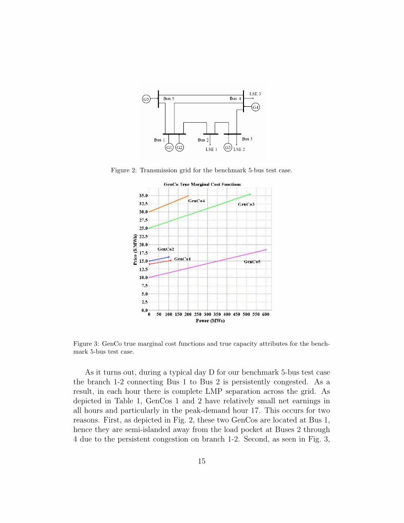
Figure 2: Transmission grid for the benchmark 5-bus test case.

Figure 3: GenCo true marginal cost functions and true capacity attributes for the bench-mark 5-bus test case.

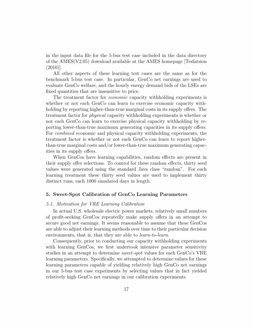
As it turns out, during a typical day D for our benchmark 5-bus test casethe branch 1-2 connecting Bus 1 to Bus 2 is persistently congested. As aresult, in each hour there is complete LMP separation across the grid. Asdepicted in Table 1, GenCos 1 and 2 have relatively small net earnings inall hours and particularly in the peak-demand hour 17. This occurs for tworeasons. First, as depicted in Fig. 2, these two GenCos are located at Bus 1,hence they are semi-islanded away from the load pocket at Buses 2 through4 due to the persistent congestion on branch 1-2. Second, as seen in Fig. 3,

15

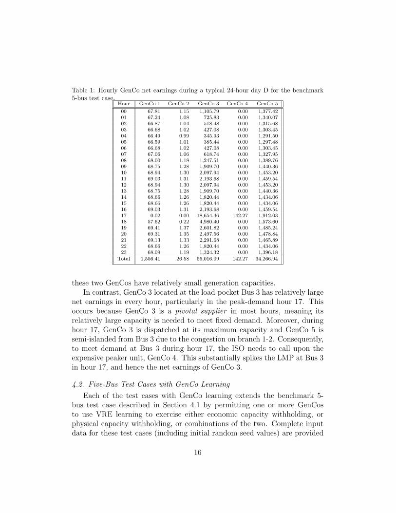
Table 1: Hourly GenCo net earnings during a typical 24-hour day D for the benchmark5-bus test case.

Hour GenCo 1 GenCo 2 GenCo 3 GenCo 4 GenCo 5

00 67.81 1.15 1,105.79 0.00 1,377.4201 67.24 1.08 725.83 0.00 1,340.0702 66.87 1.04 518.48 0.00 1,315.6803 66.68 1.02 427.08 0.00 1,303.4504 66.49 0.99 345.93 0.00 1,291.5005 66.59 1.01 385.44 0.00 1,297.4806 66.68 1.02 427.08 0.00 1,303.4507 67.06 1.06 618.74 0.00 1,327.9508 68.00 1.18 1,247.51 0.00 1,389.7609 68.75 1.28 1,909.70 0.00 1,440.3610 68.94 1.30 2,097.94 0.00 1,453.2011 69.03 1.31 2,193.68 0.00 1,459.5412 68.94 1.30 2,097.94 0.00 1,453.2013 68.75 1.28 1,909.70 0.00 1,440.3614 68.66 1.26 1,820.44 0.00 1,434.0615 68.66 1.26 1,820.44 0.00 1,434.0616 69.03 1.31 2,193.68 0.00 1,459.5417 0.02 0.00 18,654.46 142.27 1,912.0318 57.62 0.22 4,980.40 0.00 1,573.6019 69.41 1.37 2,601.82 0.00 1,485.2420 69.31 1.35 2,497.56 0.00 1,478.8421 69.13 1.33 2,291.68 0.00 1,465.8922 68.66 1.26 1,820.44 0.00 1,434.0623 68.09 1.19 1,324.32 0.00 1,396.18

Total 1,556.41 26.58 56,016.09 142.27 34,266.94

these two GenCos have relatively small generation capacities.In contrast, GenCo 3 located at the load-pocket Bus 3 has relatively large

net earnings in every hour, particularly in the peak-demand hour 17. Thisoccurs because GenCo 3 is a pivotal supplier in most hours, meaning itsrelatively large capacity is needed to meet fixed demand. Moreover, duringhour 17, GenCo 3 is dispatched at its maximum capacity and GenCo 5 issemi-islanded from Bus 3 due to the congestion on branch 1-2. Consequently,to meet demand at Bus 3 during hour 17, the ISO needs to call upon theexpensive peaker unit, GenCo 4. This substantially spikes the LMP at Bus 3in hour 17, and hence the net earnings of GenCo 3.

4.2. Five-Bus Test Cases with GenCo Learning

Each of the test cases with GenCo learning extends the benchmark 5-bus test case described in Section 4.1 by permitting one or more GenCosto use VRE learning to exercise either economic capacity withholding, orphysical capacity withholding, or combinations of the two. Complete inputdata for these test cases (including initial random seed values) are provided

16

in the input data file for the 5-bus test case included in the data directoryof the AMES(V2.05) download available at the AMES homepage [Tesfatsion(2010)].

All other aspects of these learning test cases are the same as for thebenchmark 5-bus test case. In particular, GenCo net earnings are used toevaluate GenCo welfare, and the hourly energy demand bids of the LSEs arefixed quantities that are insensitive to price.

The treatment factor for economic capacity withholding experiments iswhether or not each GenCo can learn to exercise economic capacity with-holding by reporting higher-than-true marginal costs in its supply offers. Thetreatment factor for physical capacity withholding experiments is whether ornot each GenCo can learn to exercise physical capacity withholding by re-porting lower-than-true maximum generating capacities in its supply offers.For combined economic and physical capacity withholding experiments, thetreatment factor is whether or not each GenCo can learn to report higher-than-true marginal costs and/or lower-than-true maximum generating capac-ities in its supply offers.

When GenCos have learning capabilities, random effects are present intheir supply offer selections. To control for these random effects, thirty seedvalues were generated using the standard Java class “random”. For eachlearning treatment these thirty seed values are used to implement thirtydistinct runs, each 1000 simulated days in length.

5. Sweet-Spot Calibration of GenCo Learning Parameters

5.1. Motivation for VRE Learning Calibration

In actual U.S. wholesale electric power markets, relatively small numbersof profit-seeking GenCos repeatedly make supply offers in an attempt tosecure good net earnings. It seems reasonable to assume that these GenCosare able to adjust their learning methods over time to their particular decisionenvironments, that is, that they are able to learn-to-learn.

Consequently, prior to conducting our capacity withholding experimentswith learning GenCos, we first undertook intensive parameter sensitivitystudies in an attempt to determine sweet-spot values for each GenCo’s VRElearning parameters. Specifically, we attempted to determine values for theselearning parameters capable of yielding relatively high GenCo net earningsin our 5-bus test case experiments by selecting values that in fact yieldedrelatively high GenCo net earnings in our calibration experiments.

17

In this section we briefly report on these calibration experiments, rele-gating technical details to Appendix C. In particular, we highlight severalinteresting implications regarding the importance of learning and learning-to-learn in complicated decision environments as exemplified by our currentwholesale electric power market setting.

5.2. Calibration of VRE Learning Parameters

As detailed in Appendix B, the VRE learning method used to implementlearning for each GenCo i depends on four key parameters: (qi(1), Ti, ri, ei).We first briefly summarize the role of each parameter in the learning process.

The initial propensity level qi(1) is a measure of GenCo i’s net earn-ings aspirations at the beginning of the initial day 1, which the VRE learn-ing method then successively updates in an action-conditioned manner asGenCo i successively selects new actions (supply offers) and new rewards(own-net earnings outcomes) are realized. After each updating, these action-conditioned propensities are transformed into action-conditioned probabilityassessments which GenCo i uses to select its next supply offer to report tothe ISO. The temperature parameter Ti (which has nothing to do with ac-tual weather) enters into the mapping from propensities to probabilities ina manner that affects the extent to which GenCo i experiments with newactions, particularly in early learning stages. Larger (“hotter”) values of Ti

encourage increased experimentation.The recency parameter ri enters into the propensity updating relationship;

higher values of ri dampen the rate at which GenCo i’s action-conditionedpropensities change over time. The experimentation parameter ei also entersinto the propensity updating relationship; higher values of ei permit thereinforcement effects of rewards to spill over in greater proportion from chosento non-chosen actions, thus encouraging GenCo i to experiment across abroader range of actions.

For the calibration of the recency and experimentation parameters (ri,ei),we relied on the sensitivity findings reported by Pentapalli (2008) for 3-busand 5-bus wholesale electric power market experiments. For the calibrationof the initial propensity and temperature parameters (qi(1),Ti), we used 5-bus experiments to determine GenCo net earnings for a range of positivevalues for αi and βi, defined as follows:

• αi = qi(1)/MaxDNEi, where MaxDNEi denotes GenCo i’s (positive)estimated maximum possible daily net earnings as determined struc-

18

turally from its action domain of feasible supply offers and its truemarginal cost function;

• βi = qi(1)/Ti.

5.3. Illustrative Calibration Findings

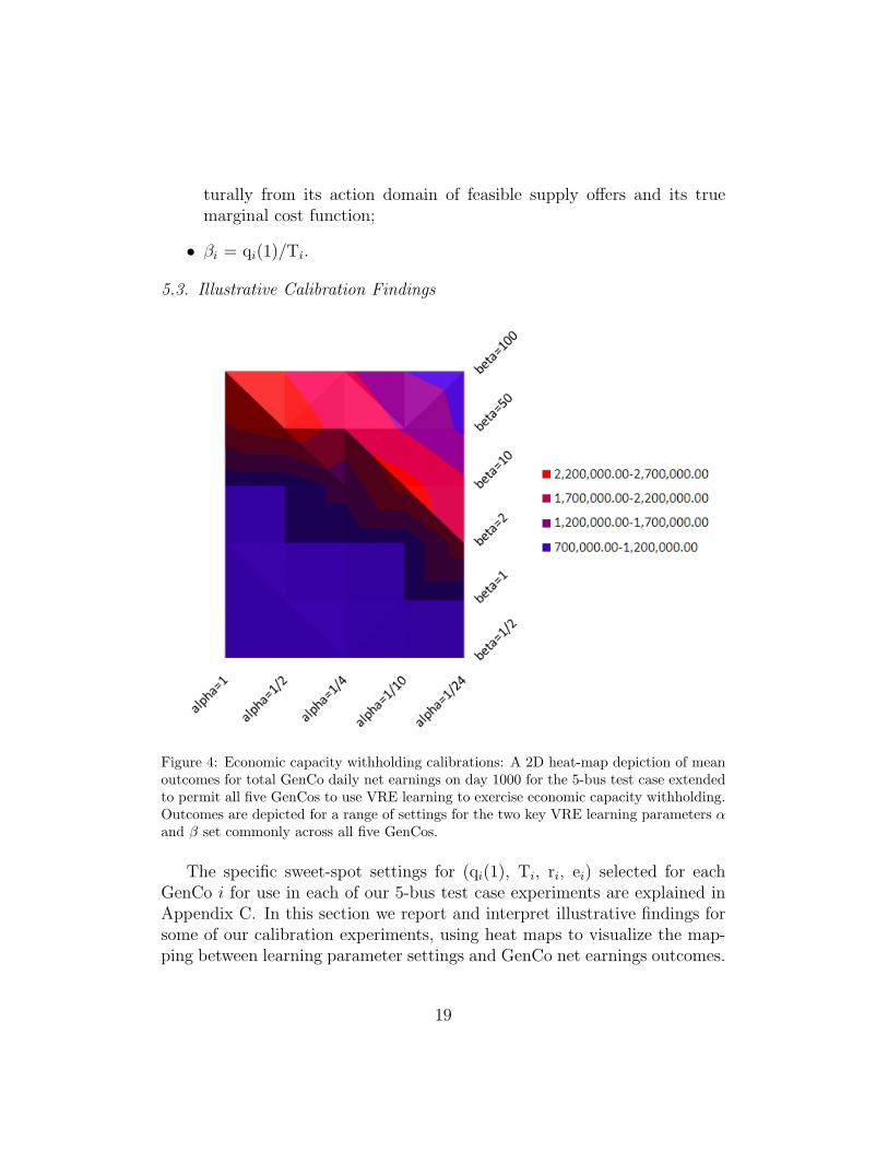
Figure 4: Economic capacity withholding calibrations: A 2D heat-map depiction of meanoutcomes for total GenCo daily net earnings on day 1000 for the 5-bus test case extendedto permit all five GenCos to use VRE learning to exercise economic capacity withholding.Outcomes are depicted for a range of settings for the two key VRE learning parameters αand β set commonly across all five GenCos.

The specific sweet-spot settings for (qi(1), Ti, ri, ei) selected for eachGenCo i for use in each of our 5-bus test case experiments are explained inAppendix C. In this section we report and interpret illustrative findings forsome of our calibration experiments, using heat maps to visualize the map-ping between learning parameter settings and GenCo net earnings outcomes.

19

Figure 4 depicts calibration-experiment findings for mean total GenCodaily net earnings attained for a 5-bus case in which each GenCo is a VRElearner able to exercise pure economic capacity withholding. The findingsare generated for a range of values for α and β, commonly set across allGenCos. An interesting pattern is immediately evident: namely, the (α,β)combinations associated with the highest mean net earnings outcomes liealong a nonlinear ridge line that traverses from (1, 100) in the northwestcorner to (1/24, 2) in the south-central region. What causes this nonlinearcoupled dependence of mean net earnings outcomes on α and β?

The settings for α and β have distinct but correlated effects on the degreeto which each GenCo experiments with different actions, i.e., with differentsupply offers (reported marginal cost functions). All else equal, high α valuesreflecting optimistically high initial net earnings expectations tend to induceexperimentation with many different actions due to “disappointment” withthe net earnings outcomes that result from each choice. Conversely, low αvalues reflecting pessimistically low initial net earnings expectations tend toinduce premature fixation on an early chosen action due to the “surprisinglyhigh” net earnings that result from this choice.

High β values reflecting high cooling levels (low temperature parametersettings) amplify the tendency to premature fixation in the case of low αvalues by amplifying differences in propensity levels across action choices.Moderately low β values can prevent premature fixation by dampening theeffects of propensity differences on action choice probabilities.

However, extremely low β values result in action choice probability dis-tributions that are essentially uniform across each GenCo’s action domain,negating all GenCo efforts to learn which actions result in the highest dailynet earnings. In this case the behavior of the GenCos corresponds to Gode-Sunder (1993,1997) budget-constrained zero-intelligence (ZI-B) market sell-ers who randomly select supply offers subject only to a budget constraint.That is, each GenCo randomly chooses supply offers from its action domain,which by construction only includes possible reported marginal cost functionsthat lie on or above the GenCo’s true marginal cost function (thus enforcinga break-even constraint). The deleterious effect of this ZI-B GenCo behavioris seen in the uniformly low mean net earnings outcomes achieved in Fig. 4for the lowest tested β levels 1/2 and 1.

The bottom line following from the calibration-experiment findings re-ported in Fig. 4 is that the learning representation for the GenCos definitelymatters. GenCos achieve their highest mean net earnings along a nonlinear

20

ridge-line of sweet-spot (α, β) values traversing from (1, 100) to (1/24, 2),and their lowest mean net earnings for extremely low β values that inducethe GenCos to behave like Gode-Sunder ZI-B market sellers.

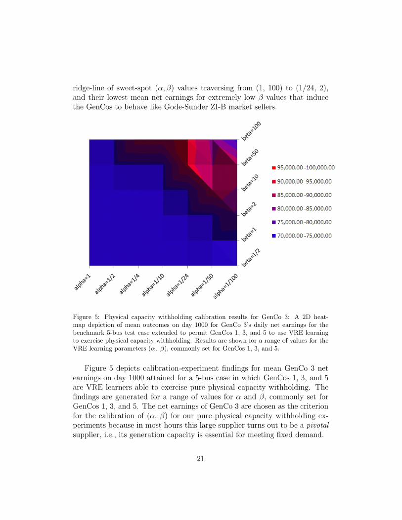
Figure 5: Physical capacity withholding calibration results for GenCo 3: A 2D heat-map depiction of mean outcomes on day 1000 for GenCo 3’s daily net earnings for thebenchmark 5-bus test case extended to permit GenCos 1, 3, and 5 to use VRE learningto exercise physical capacity withholding. Results are shown for a range of values for theVRE learning parameters (α, β), commonly set for GenCos 1, 3, and 5.

Figure 5 depicts calibration-experiment findings for mean GenCo 3 netearnings on day 1000 attained for a 5-bus case in which GenCos 1, 3, and 5are VRE learners able to exercise pure physical capacity withholding. Thefindings are generated for a range of values for α and β, commonly set forGenCos 1, 3, and 5. The net earnings of GenCo 3 are chosen as the criterionfor the calibration of (α, β) for our pure physical capacity withholding ex-periments because in most hours this large supplier turns out to be a pivotalsupplier, i.e., its generation capacity is essential for meeting fixed demand.

21

Three interesting observations can be made about the results reported inFig. 5. First, learning matters: the setting for (α, β) substantially affectsmean GenCo 3 net earnings. Second, the sweet-spot (α, β) combinationsassociated with the highest mean GenCo 3 net earnings roughly lie along avertical ridge line ranging from (1/24, 50) to (1/24, 100). Third, comparingthe pure physical capacity withholding outcomes in Figure 5 with the pureeconomic capacity withholding outcomes in Figure 4, it is seen that the sweet-spot region for GenCo 3’s (α, β) learning parameters strongly depends onthe particular learning environment.

This third finding indicates the importance of learning-to-learn. No onesetting for the parameters of a learning method can be expected to do wellacross all possible decision environments in which the learning method mightbe applied.

6. Test-Case Findings for Pure Economic Capacity Withholding

This section reports findings for two types of 5-bus test case experiments.The first type of experiment tests the extent to which a single GenCo canlearn to achieve higher net earnings through economic capacity withholdingwhen all other GenCos report their true cost and capacity attributes to theISO. The second type of experiment tests the extent to which two GenCoscan co-learn over time to achieve higher net earnings through economic ca-pacity withholding when all other GenCos report their true cost and capacityattributes to the ISO.

Of particular interest is the extent to which the second type of experi-ment results in correlated supply offer selections and correlated net earningsoutcomes for the two learning GenCos.

6.1. Economic Capacity Withholding by One Learning GenCo

GenCo 3 is selected as the sole learner for this first type of experimentbecause of the critical role it plays in the determination of locational marginalprices (LMPs). This critical role results for three reasons: (a) GenCo 3 has arelatively large generation capacity; (b) GenCo 3 is a pivotal supplier duringpeak (high) demand hours, meaning that its capacity is needed to meetLSE fixed demand; and (c) GenCo 3’s true marginal costs of production arerelatively high.

As carefully explained in Appendix A, each supply offer reported to theISO by a learning GenCo takes the form of a reported linear marginal cost

22

function with ordinate aR and slope 2bR. This function is defined over areported generation capacity interval ranging from 0 to a reported maximumgeneration capacity CapRU .

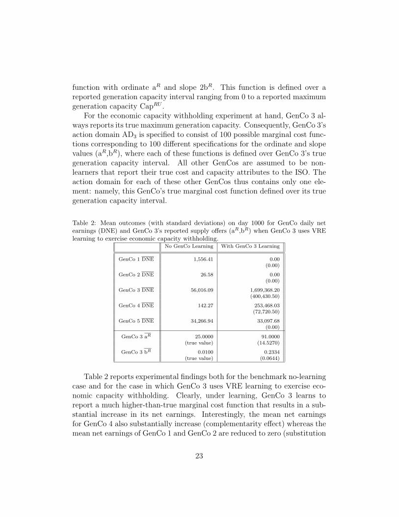
For the economic capacity withholding experiment at hand, GenCo 3 al-ways reports its true maximum generation capacity. Consequently, GenCo 3’saction domain AD3 is specified to consist of 100 possible marginal cost func-tions corresponding to 100 different specifications for the ordinate and slopevalues (aR,bR), where each of these functions is defined over GenCo 3’s truegeneration capacity interval. All other GenCos are assumed to be non-learners that report their true cost and capacity attributes to the ISO. Theaction domain for each of these other GenCos thus contains only one ele-ment: namely, this GenCo’s true marginal cost function defined over its truegeneration capacity interval.

Table 2: Mean outcomes (with standard deviations) on day 1000 for GenCo daily netearnings (DNE) and GenCo 3’s reported supply offers (aR,bR) when GenCo 3 uses VRElearning to exercise economic capacity withholding.

No GenCo Learning With GenCo 3 Learning

GenCo 1 DNE 1,556.41 0.00(0.00)

GenCo 2 DNE 26.58 0.00(0.00)

GenCo 3 DNE 56,016.09 1,699,368.20(400,430.50)

GenCo 4 DNE 142.27 253,468.03(72,720.50)

GenCo 5 DNE 34,266.94 33,097.68(0.00)

GenCo 3 aR 25.0000 91.0000(true value) (14.5270)

GenCo 3 bR 0.0100 0.2334(true value) (0.0644)

Table 2 reports experimental findings both for the benchmark no-learningcase and for the case in which GenCo 3 uses VRE learning to exercise eco-nomic capacity withholding. Clearly, under learning, GenCo 3 learns toreport a much higher-than-true marginal cost function that results in a sub-stantial increase in its net earnings. Interestingly, the mean net earningsfor GenCo 4 also substantially increase (complementarity effect) whereas themean net earnings of GenCo 1 and GenCo 2 are reduced to zero (substitution

23

effect), even though GenCos 4, 1, and 2 are not learning agents and hencealways report their true cost and capacity attributes to the ISO.

The reason for these findings is as follows. The branch from Bus 1 to Bus 2is persistently congested whether or not GenCo 3 has learning capabilities.However, under learning, GenCo 3’s high reported marginal costs duringthe peak-demand hour 17 results in the higher dispatch of GenCo 4 (to maxcapacity) and also in the higher dispatch of GenCo 5 in order to meet demandin the load pocket surrounding GenCo 3 at Bus 3. GenCo 1 and GenCo 2have to be backed down to 0 in order to permit GenCo 5 to be called up toservice this demand without overloading the branch from Bus 1 to Bus 2.

As noted in the introduction, these complicated substitution and comple-mentarity effects arising through network interactions are not well capturedusing traditional derivative measures [Bulow et al. (1985)].

6.2. Economic Capacity Withholding by Two Co-Learning GenCos

Two different pairs of co-learning GenCos are examined for this secondtype of experiment: Case (1) GenCo 1 and GenCo 3; and Case (2) GenCo 3and GenCo 5. The reason for these choices is as follows.

For Case (1), GenCo 1 is a small GenCo with relatively low true marginalcost whereas GenCo 3 is a pivotal supplier during peak-demand hours withrelatively high true marginal costs. Can GenCo 1 learn to “free ride” on themarket power exercised by GenCo 3 in order to improve its net earnings?For Case (2), GenCo 3 and GenCo 5 both have relatively large maximumgeneration capacities, but GenCo 5 has relatively lower marginal costs. CanGenCo 5 learn to undercut GenCo 3’s supply offers when GenCo 3 reportsaggressively high supply offers, thus raising its net earnings?

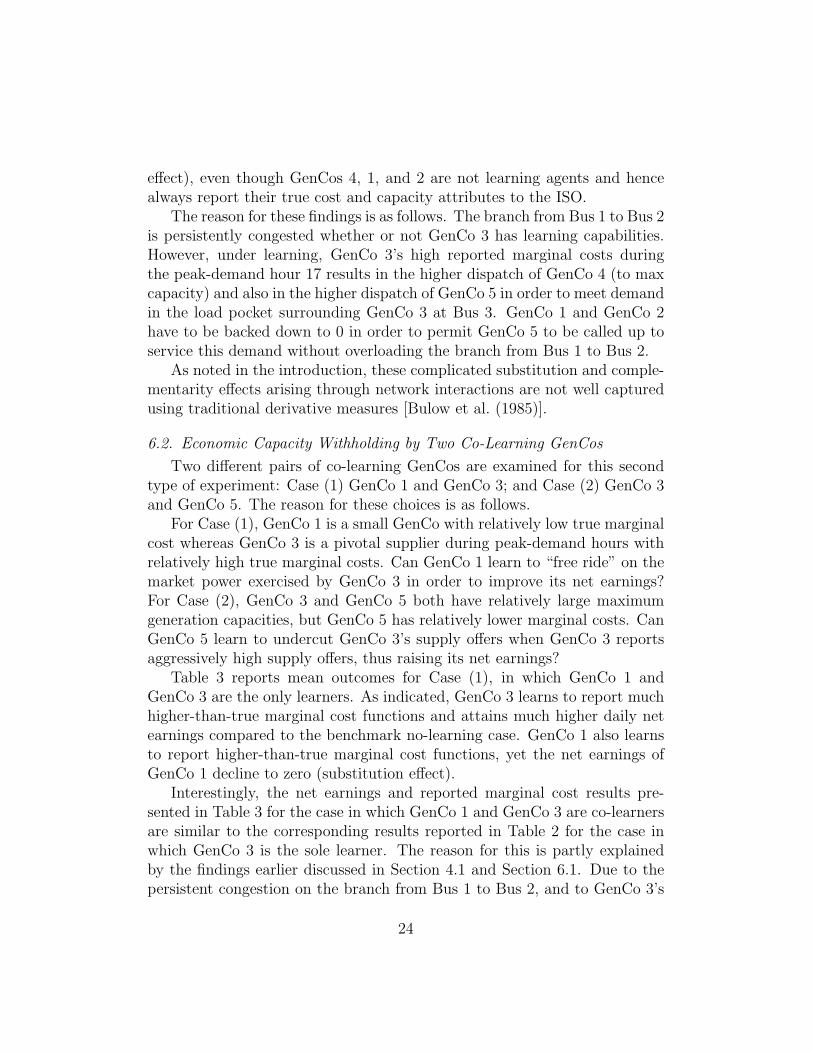
Table 3 reports mean outcomes for Case (1), in which GenCo 1 andGenCo 3 are the only learners. As indicated, GenCo 3 learns to report muchhigher-than-true marginal cost functions and attains much higher daily netearnings compared to the benchmark no-learning case. GenCo 1 also learnsto report higher-than-true marginal cost functions, yet the net earnings ofGenCo 1 decline to zero (substitution effect).

Interestingly, the net earnings and reported marginal cost results pre-sented in Table 3 for the case in which GenCo 1 and GenCo 3 are co-learnersare similar to the corresponding results reported in Table 2 for the case inwhich GenCo 3 is the sole learner. The reason for this is partly explainedby the findings earlier discussed in Section 4.1 and Section 6.1. Due to thepersistent congestion on the branch from Bus 1 to Bus 2, and to GenCo 3’s

24

relatively large generation capacity, GenCo 3 is a pivotal supplier in mosthours, meaning that its capacity is needed to meet fixed demand. On theother hand, GenCo 1 is a relatively small unit located on the “wrong” side ofthe congested branch 1-2 and it typically fails to be dispatched at any posi-tive level. The result is that GenCo 3’s reported supply offers have a muchgreater effect on dispatch results. GenCo 3 learns to take advantage of thissituation by raising its reported marginal costs, resulting in an increase in theLMP at its Bus 3. In contrast, despite its learning capabilities, GenCo 1’ssupply offers are essentially irrelevant for the determination of price levels,as well as for the determination of GenCo 3’s reported supply offers.

Table 3: Mean outcomes (with standard deviations) on day 1000 for GenCo daily netearnings (DNE), and for reported supply offers (aR,bR) for GenCo 1 and GenCo 3, whenboth GenCo 1 and GenCo 3 use VRE learning to exercise economic capacity withholding.

No GenCo Learning With GenCo 1, 3 Learning

GenCo 1 DNE 1,556.41 0.00(0.00)

GenCo 2 DNE 26.58 0.00(0.00)

GenCo 3 DNE 56,016.09 1,699,368.20(400,430.50)

GenCo 4 DNE 142.27 253,468.03(72,720.50)

GenCo 5 DNE 34,266.94 33,097.68(0.00)





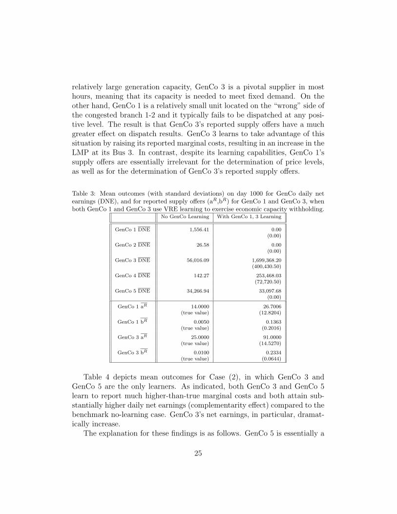
Table 4 depicts mean outcomes for Case (2), in which GenCo 3 andGenCo 5 are the only learners. As indicated, both GenCo 3 and GenCo 5learn to report much higher-than-true marginal costs and both attain sub-stantially higher daily net earnings (complementarity effect) compared to thebenchmark no-learning case. GenCo 3’s net earnings, in particular, dramat-ically increase.

The explanation for these findings is as follows. GenCo 5 is essentially a

25

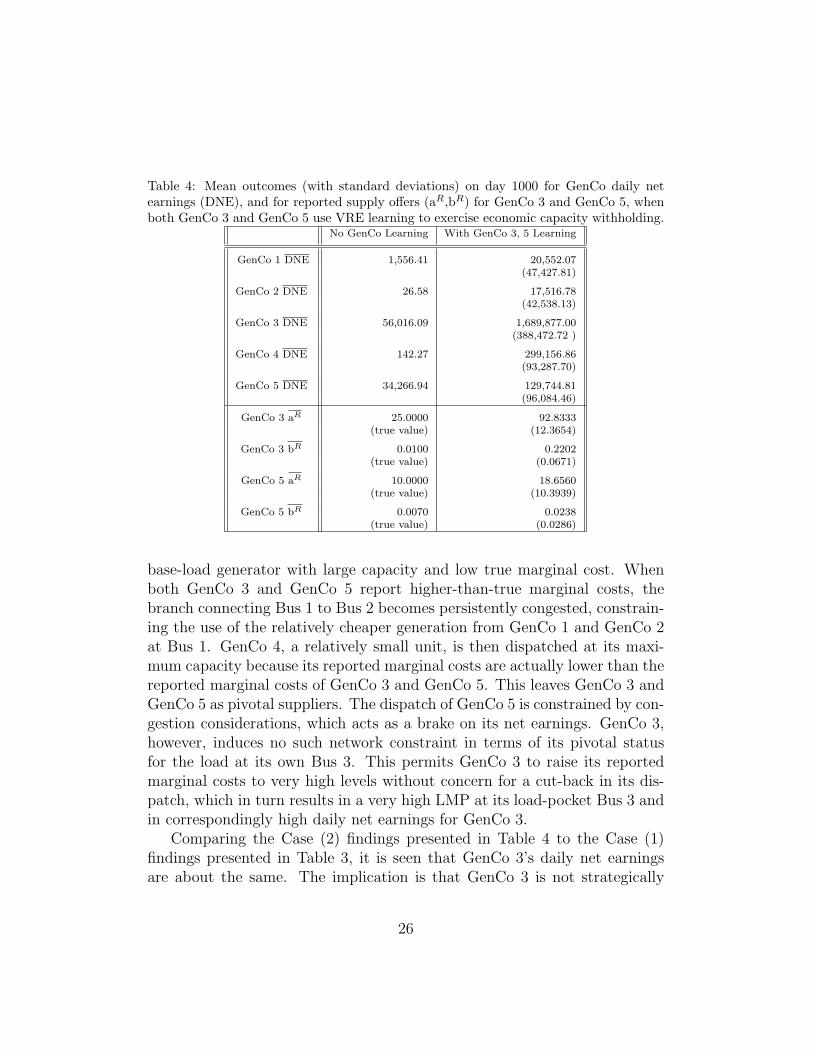
Table 4: Mean outcomes (with standard deviations) on day 1000 for GenCo daily netearnings (DNE), and for reported supply offers (aR,bR) for GenCo 3 and GenCo 5, whenboth GenCo 3 and GenCo 5 use VRE learning to exercise economic capacity withholding.

No GenCo Learning With GenCo 3, 5 Learning

GenCo 1 DNE 1,556.41 20,552.07(47,427.81)

GenCo 2 DNE 26.58 17,516.78(42,538.13)

GenCo 3 DNE 56,016.09 1,689,877.00(388,472.72 )

GenCo 4 DNE 142.27 299,156.86(93,287.70)

GenCo 5 DNE 34,266.94 129,744.81(96,084.46)





base-load generator with large capacity and low true marginal cost. Whenboth GenCo 3 and GenCo 5 report higher-than-true marginal costs, thebranch connecting Bus 1 to Bus 2 becomes persistently congested, constrain-ing the use of the relatively cheaper generation from GenCo 1 and GenCo 2at Bus 1. GenCo 4, a relatively small unit, is then dispatched at its maxi-mum capacity because its reported marginal costs are actually lower than thereported marginal costs of GenCo 3 and GenCo 5. This leaves GenCo 3 andGenCo 5 as pivotal suppliers. The dispatch of GenCo 5 is constrained by con-gestion considerations, which acts as a brake on its net earnings. GenCo 3,however, induces no such network constraint in terms of its pivotal statusfor the load at its own Bus 3. This permits GenCo 3 to raise its reportedmarginal costs to very high levels without concern for a cut-back in its dis-patch, which in turn results in a very high LMP at its load-pocket Bus 3 andin correspondingly high daily net earnings for GenCo 3.

Comparing the Case (2) findings presented in Table 4 to the Case (1)findings presented in Table 3, it is seen that GenCo 3’s daily net earningsare about the same. The implication is that GenCo 3 is not strategically

26

interacting with GenCo 5 in Case (2); it behaves essentially the same waywhether or not GenCo 5 has learning capabilities. On the other hand, inCase (2) GenCo 5 is able to take advantage of GenCo 3’s economic capacitywithholding to raise its own reported marginal costs without risking a cut-back in its dispatch, which substantially increases its daily net earnings.

Case (2) also differs from Case (1) in another interesting way. In Case (2),GenCo 5 ends up reporting marginal costs that are higher than the marginalcosts of the non-learning GenCos 1 and 2. As a result, GenCo 1 and GenCo 2located at Bus 1 are now dispatched at positive levels even though the branchconnecting Bus 1 to Bus 2 is persistently congested. Consequently, these non-learning GenCos are better off in Case (2) than in Case (1).

7. Test-Case Findings for Pure Physical Capacity Withholding

In parallel with Section 6, this section considers two types of experiments.The first type of experiment tests the extent to which a single GenCo canlearn to achieve higher net earnings through physical capacity withholdingwhen all other GenCos report their true cost and capacity attributes to theISO. The second type of experiment tests the extent to which two GenCoscan co-learn over time to achieve higher net earnings through physical capac-ity withholding when all other GenCos report their true cost and capacityattributes to the ISO. Of particular interest is the extent to which the secondtype of experiment results in correlated supply offer selections and correlatednet earnings outcomes for the two learning GenCos.

The treatment factor for these experiments is the maximum possibleshrinkage for reported maximum generation capacity that a learning GenCocan submit to the ISO, the interpretation being that any larger shrinkagewould risk detection by the ISO. The tested ranges for this treatment factorare chosen to avoid supply inadequacy, i.e., the reporting of capacities thatare insufficient to meet total fixed demand.

7.1. Physical Capacity Withholding by One Learning GenCo

In the experiments presented in this section, as in Section 6.1, onlyGenCo 3 has learning capabilities. Here, however, GenCo 3’s learning isrestricted to the ability to exercise physical capacity withholding. The onlytreatment factor is GenCo 3’s shrinkage value MPRMCap3, i.e., the settingfor GenCo 3’s minimum possible reported maximum capacity that determinesthe lowest possible maximum generation capacity that GenCo 3 is able to

27

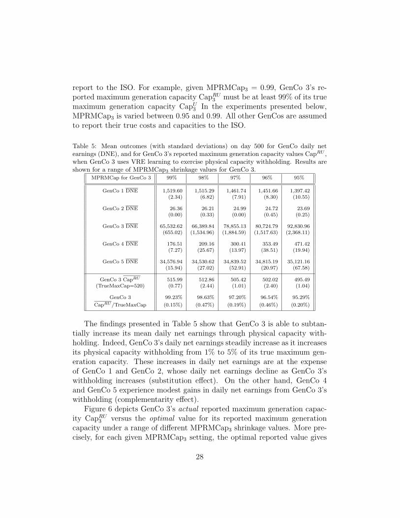
report to the ISO. For example, given MPRMCap3 = 0.99, GenCo 3’s re-ported maximum generation capacity CapRU3 must be at least 99% of its truemaximum generation capacity CapU3 In the experiments presented below,MPRMCap3 is varied between 0.95 and 0.99. All other GenCos are assumedto report their true costs and capacities to the ISO.

Table 5: Mean outcomes (with standard deviations) on day 500 for GenCo daily netearnings (DNE), and for GenCo 3’s reported maximum generation capacity values CapRU ,when GenCo 3 uses VRE learning to exercise physical capacity withholding. Results areshown for a range of MPRMCap3 shrinkage values for GenCo 3.

MPRMCap for GenCo 3 99% 98% 97% 96% 95%

GenCo 1 DNE 1,519.60 1,515.29 1,461.74 1,451.66 1,397.42(2.34) (6.82) (7.91) (8.30) (10.55)

GenCo 2 DNE 26.36 26.21 24.99 24.72 23.69(0.00) (0.33) (0.00) (0.45) (0.25)

GenCo 3 DNE 65,532.62 66,389.84 78,855.13 80,724.79 92,830.96(655.02) (1,534.96) (1,884.59) (1,517.63) (2,368.11)

GenCo 4 DNE 176.51 209.16 300.41 353.49 471.42(7.27) (25.67) (13.97) (38.51) (19.94)

GenCo 5 DNE 34,576.94 34,530.62 34,839.52 34,815.19 35,121.16(15.94) (27.02) (52.91) (20.97) (67.58)

GenCo 3 CapRU 515.99 512.86 505.42 502.02 495.49(TrueMaxCap=520) (0.77) (2.44) (1.01) (2.40) (1.04)

GenCo 3 99.23% 98.63% 97.20% 96.54% 95.29%

CapRU/TrueMaxCap (0.15%) (0.47%) (0.19%) (0.46%) (0.20%)

The findings presented in Table 5 show that GenCo 3 is able to subtan-tially increase its mean daily net earnings through physical capacity with-holding. Indeed, GenCo 3’s daily net earnings steadily increase as it increasesits physical capacity withholding from 1% to 5% of its true maximum gen-eration capacity. These increases in daily net earnings are at the expenseof GenCo 1 and GenCo 2, whose daily net earnings decline as GenCo 3’swithholding increases (substitution effect). On the other hand, GenCo 4and GenCo 5 experience modest gains in daily net earnings from GenCo 3’swithholding (complementarity effect).

Figure 6 depicts GenCo 3’s actual reported maximum generation capac-ity CapRU3 versus the optimal value for its reported maximum generationcapacity under a range of different MPRMCap3 shrinkage values. More pre-cisely, for each given MPRMCap3 setting, the optimal reported value gives

28

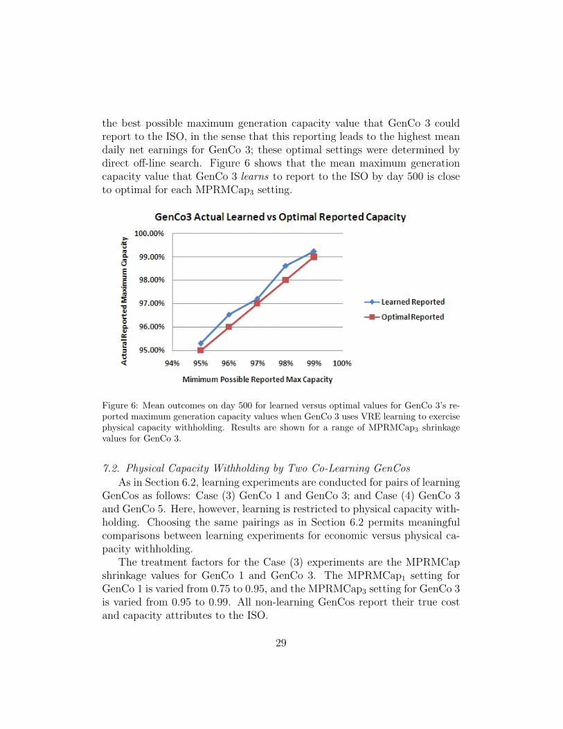
the best possible maximum generation capacity value that GenCo 3 couldreport to the ISO, in the sense that this reporting leads to the highest meandaily net earnings for GenCo 3; these optimal settings were determined bydirect off-line search. Figure 6 shows that the mean maximum generationcapacity value that GenCo 3 learns to report to the ISO by day 500 is closeto optimal for each MPRMCap3 setting.

Figure 6: Mean outcomes on day 500 for learned versus optimal values for GenCo 3’s re-ported maximum generation capacity values when GenCo 3 uses VRE learning to exercisephysical capacity withholding. Results are shown for a range of MPRMCap3 shrinkagevalues for GenCo 3.

7.2. Physical Capacity Withholding by Two Co-Learning GenCos

As in Section 6.2, learning experiments are conducted for pairs of learningGenCos as follows: Case (3) GenCo 1 and GenCo 3; and Case (4) GenCo 3and GenCo 5. Here, however, learning is restricted to physical capacity with-holding. Choosing the same pairings as in Section 6.2 permits meaningfulcomparisons between learning experiments for economic versus physical ca-pacity withholding.

The treatment factors for the Case (3) experiments are the MPRMCapshrinkage values for GenCo 1 and GenCo 3. The MPRMCap1 setting forGenCo 1 is varied from 0.75 to 0.95, and the MPRMCap3 setting for GenCo 3is varied from 0.95 to 0.99. All non-learning GenCos report their true costand capacity attributes to the ISO.

29

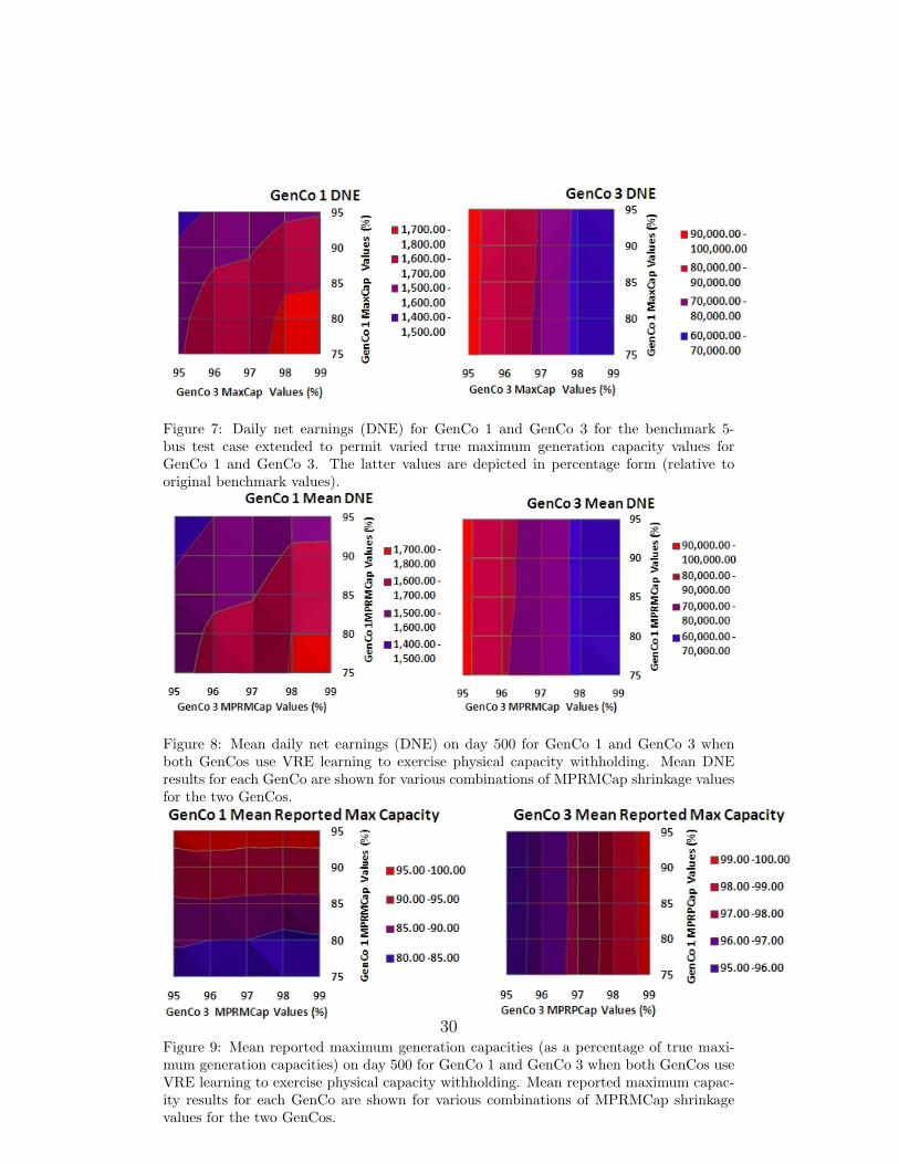
Figure 7: Daily net earnings (DNE) for GenCo 1 and GenCo 3 for the benchmark 5-bus test case extended to permit varied true maximum generation capacity values forGenCo 1 and GenCo 3. The latter values are depicted in percentage form (relative tooriginal benchmark values).

Figure 8: Mean daily net earnings (DNE) on day 500 for GenCo 1 and GenCo 3 whenboth GenCos use VRE learning to exercise physical capacity withholding. Mean DNEresults for each GenCo are shown for various combinations of MPRMCap shrinkage valuesfor the two GenCos.

Figure 9: Mean reported maximum generation capacities (as a percentage of true maxi-mum generation capacities) on day 500 for GenCo 1 and GenCo 3 when both GenCos useVRE learning to exercise physical capacity withholding. Mean reported maximum capac-ity results for each GenCo are shown for various combinations of MPRMCap shrinkagevalues for the two GenCos.

30

As a benchmark of comparison for Case (3), Figure 7 presents typical dailynet earnings for GenCo 1 and GenCo 3 for the benchmark 5-bus test case(no learning) extended to permit a range of settings for the true maximumgeneration capacities of GenCo 1 and GenCo 3. From these findings it canbe seen that GenCo 1, a relatively small unit, does best when its maximumgeneration capacity is 75% of its benchmark maximum generation capacityand the maximum generation capacity of the relatively large GenCo 3 is99% of its benchmark maximum generation capacity. In contrast, GenCo 3does best when its maximum generation capacity is 95% of its benchmarkmaximum generation capacity no matter what value is set for GenCo 1’smaximum generation capacity.

Figure 8 presents mean daily net earnings for GenCo 1 and GenCo 3 onday 5000 when both GenCos use VRE learning to exercise physical capacitywithholding. From the left-hand side of this figure, it is seen that GenCo 1attains its highest mean daily net earnings when its MPRMCap1 shrinkagevalue is set at its lowest tested level (0.75) and the MPRMCap3 shrinkagevalue for GenCo 3 is set at its highest tested level (0.99). Comparing theleft-hand side of Figure 8 to the left-hand side of Figure 7, it is also seenthat the MPRMCap1 region over which GenCo 1 attains its highest meandaily net earnings under learning is smaller than the maximum generationcapacity region over which it attains its highest daily net earnings in thebenchmark no-learning case.

Interestingly, in parallel with the no-learning findings reported in Fig-ure 7, it is seen in the right-hand side of Figure 8 that GenCo 3 attainsits highest mean daily net earnings when its MPRMCap3 shrinkage value isset at its lowest tested level (0.95). Also, the vertically-striped pattern forGenCo 3’s mean daily net earnings indicates that GenCo 1’s MPRMCap1 set-tings have essentially no effect on the daily net earnings attained by GenCo 3.

Figure 9 displays mean reported maximum generation capacities (as apercentage of benchmark true maximum generation capacities) for GenCo 1and GenCo 3 on day 500 when both these GenCos use VRE learning to ex-ercise physical capacity withholding. From the left-hand side of the figure,it is seen that GenCo 1’s mean reported maximum generation capacity issomewhat higher than its MPRMCap1 shrinkage value for each tested pairof MPRMCap settings for GenCo 1 and GenCo 3. Moreover, as indicatedby the horizontally-striped pattern in GenCo 1’s reported maximum capacityresults, GenCo 3’s reported maximum generation capacity choices have essen-tially no effect on the reported maximum generation capacity choices made by

31

GenCo 1. As indicated in the right-hand side of the figure, GenCo 3’s meanreported maximum generation capacity is close to its MPRMCap3 shrinkagevalue for each tested pair of MPRMCap settings for GenCo 1 and 3. More-over, as indicated by the vertically-striped pattern in GenCo 3’s reportedmaximum generation capacity results, GenCo 1’s reported maximum gener-ation capacity choices have essentially no effect on the reported maximumgeneration capacity choices made by GenCo 3.

In summary, in the Case (3) physical capacity withholding experiments inwhich only GenCo 1 and GenCo 3 are learners, the smaller GenCo 1 is ableto attain higher net earnings by essentially free riding on the strategic phys-ical capacity reporting of the larger GenCo 3 (complementarity effect). Incontrast, GenCo 3’s reported maximum generation capacity choices are essen-tially uncorrelated with the reported maximum generation capacity choicesof GenCo 1.

For the Case (4) physical capacity withholding experiments in which onlyGenCo 3 and GenCo 5 are learners, the treatment factors are the MPRMCapshrinkage values for GenCo 3 and GenCo 5. The MPRMCap3 shrinkage valuefor GenCo 3 is varied from 0.95 to 0.99, and the MPRMCap5 shrinkage valuefor GenCo 5 is varied from 0.70 to 0.95. All non-learning GenCos reporttheir true cost and capacity attributes to the ISO.

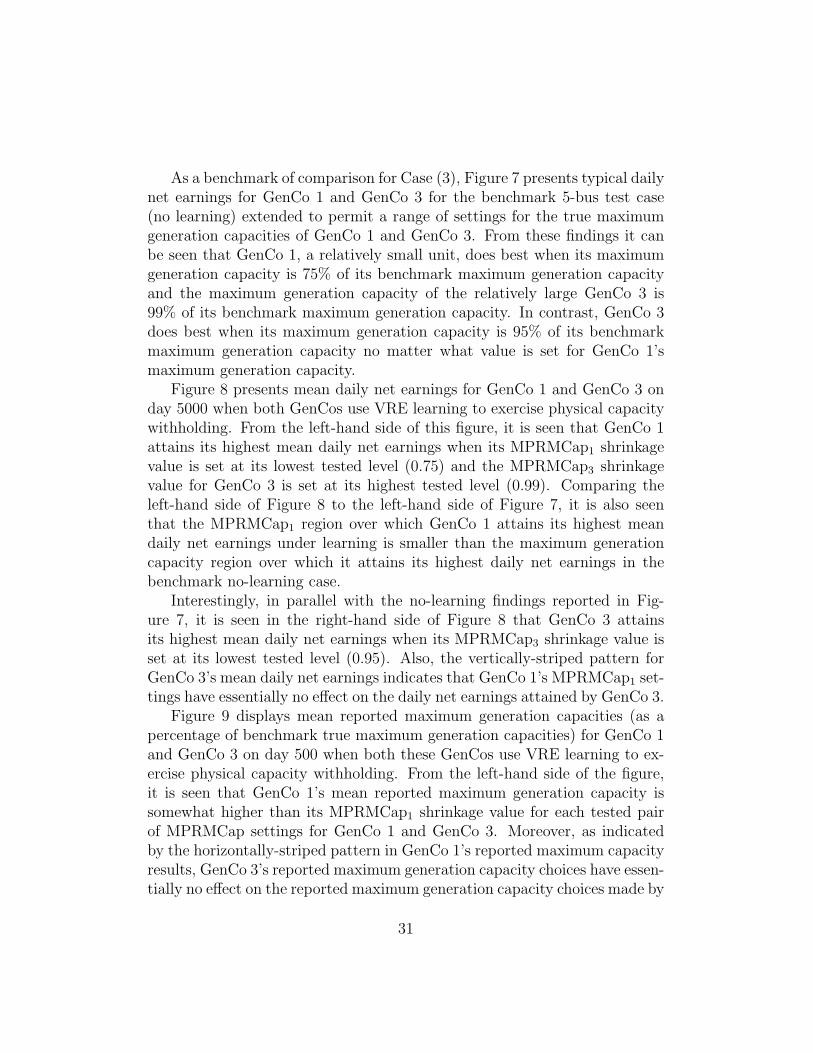
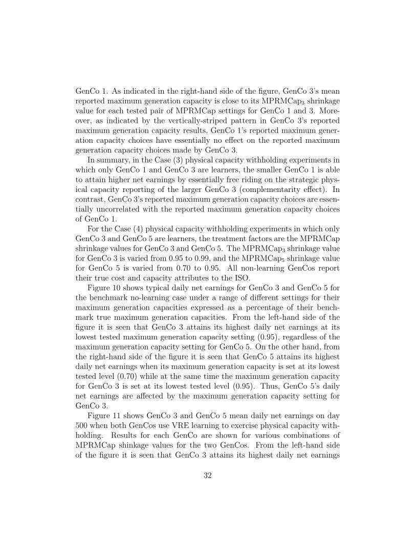
Figure 10 shows typical daily net earnings for GenCo 3 and GenCo 5 forthe benchmark no-learning case under a range of different settings for theirmaximum generation capacities expressed as a percentage of their bench-mark true maximum generation capacities. From the left-hand side of thefigure it is seen that GenCo 3 attains its highest daily net earnings at itslowest tested maximum generation capacity setting (0.95), regardless of themaximum generation capacity setting for GenCo 5. On the other hand, fromthe right-hand side of the figure it is seen that GenCo 5 attains its highestdaily net earnings when its maximum generation capacity is set at its lowesttested level (0.70) while at the same time the maximum generation capacityfor GenCo 3 is set at its lowest tested level (0.95). Thus, GenCo 5’s dailynet earnings are affected by the maximum generation capacity setting forGenCo 3.

Figure 11 shows GenCo 3 and GenCo 5 mean daily net earnings on day500 when both GenCos use VRE learning to exercise physical capacity with-holding. Results for each GenCo are shown for various combinations ofMPRMCap shinkage values for the two GenCos. From the left-hand sideof the figure it is seen that GenCo 3 attains its highest daily net earnings

32

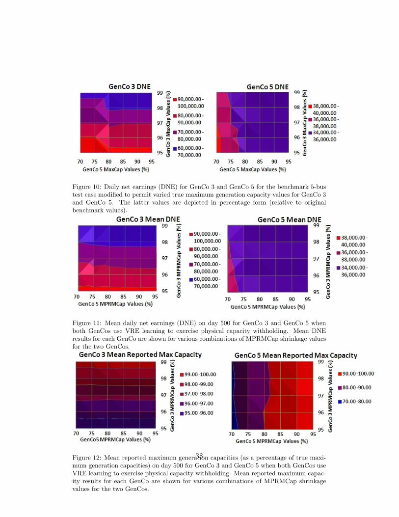
Figure 10: Daily net earnings (DNE) for GenCo 3 and GenCo 5 for the benchmark 5-bustest case modified to permit varied true maximum generation capacity values for GenCo 3and GenCo 5. The latter values are depicted in percentage form (relative to originalbenchmark values).

Figure 11: Mean daily net earnings (DNE) on day 500 for GenCo 3 and GenCo 5 whenboth GenCos use VRE learning to exercise physical capacity withholding. Mean DNEresults for each GenCo are shown for various combinations of MPRMCap shrinkage valuesfor the two GenCos.

Figure 12: Mean reported maximum generation capacities (as a percentage of true maxi-mum generation capacities) on day 500 for GenCo 3 and GenCo 5 when both GenCos useVRE learning to exercise physical capacity withholding. Mean reported maximum capac-ity results for each GenCo are shown for various combinations of MPRMCap shrinkagevalues for the two GenCos.

33

when its MPRMCap3 value is set to its lowest tested level (0.95), regardlessof the MPRMCap5 shrinkage value for GenCo 5. In contrast, from the right-hand side of the figure it is seen that GenCo 5 attains its highest daily netearnings when its MPRMCap5 shrinkage value is set to its lowest tested level(0.70) while at the same time the MPRMCap3 shrinkage value for GenCo 3is set at its lowest tested level (0.95). Consequently, in similarity to the no-learning case, GenCo 5’s daily net earnings under learning are affected bythe MPRMCap3 shrinkage value set for GenCo 3.

Figure 12 shows GenCo 3 and GenCo 5 mean reported maximum gener-ation capacities as a percentage of their true maximum generation capacitieswhen both GenCos use VRE learning to exercise physical capacity with-holding. Results for each GenCo are shown for various combinations ofMPRMCap shinkage values for the two GenCos. From the left-hand sideof the figure it is seen that GenCo 3’s mean reported maximum generationcapacity is close to its MPRMCap3 shrinkage value for each tested combi-nation of MPRMCap shrinkage values for GenCo 3 and GenCo 5. Also, thehorizonally-striped pattern of the results indicates that GenCo 5’s reportedmaximum capacities have very little effect on GenCo 3’s reported maximumcapacities. The right-hand side of the figure shows that GenCo 5’s mean re-ported maximum generation capacity is higher than its MPRMCap5 shrink-age value for each tested combination of MPRMCap shrinkage values forGenCo 3 and GenCo 5. Also, GenCo 5’s reported maximum generation ca-pacities are weakly positively correlated with GenCo 3’s reported maximumgeneration capacities (weak complementarity effect).

8. Test-Case Findings for Experiments with Combined Economicand Physical Capacity Withholding

In this section, two types of experiments are studied. The first type ofexperiment tests the extent to which a single GenCo can learn to achievehigher net earnings through economic and/or physical capacity withholdingwhen all other GenCos report their true cost and capacity attributes to theISO. The second type of experiment tests the extent to which two GenCos canco-learn over time to achieve higher net earnings through economic and/orphysical capacity withholding when all other GenCos report their true costand capacity attributes to the ISO.

34

8.1. Combined Economic and Physical Capacity Withholding by One GenCo

For reasons elaborated in earlier sections, GenCo 3 is selected as the onelearning GenCo able to learn to exercise either economic or physical capacitywithholding. Of particular interest will be whether one type of withholdingdominates the other for GenCo 3 in the sense that it yields consistently highermean daily net earnings for GenCo 3.

Table 6 presents mean outcomes (with standard deviations) on day 1000for GenCo net earnings, and for GenCo 3’s reported supply offers, for arange of MPRMCap3 shrinkage value settings for GenCo 3. It is seen thatGenCo 3 attains much higher mean daily net earnings than in the benchmarkno-learning case. Moreover, the mean daily net earnings for GenCo 3 mono-tonically increase with increases in the MPRMCap3 setting for GenCo 3.

However, comparing the findings in Table 6 with the benchmark (no learn-ing) and pure economic capacity withholding findings in Table 2, it is seenthat the increase in GenCo 3’s mean net earnings through economic capacitywithholding are substantially greater than the increases in its mean net earn-ings from successively higher physical capacity withholding. Thus, althoughboth forms of capacity withholding add to GenCo 3’s net earnings, economiccapacity withholding is the primary channel through which GenCo 3 increasesits net earnings.

8.2. Combined Economic and Physical Capacity Withholding by Two GenCos

As in Section 6.2 and Section 7.2, learning experiments are conducted fortwo co-learning GenCos: namely, GenCo 3 and GenCo 5. Here, however,the two co-learning GenCos are permitted to engage in both economic andphysical capacity withholding. All other GenCos are assumed to report theirtrue cost and capacity attributes to the ISO.

Table 7 shows mean outcomes (with standard deviations) on day 1000 forGenCo net earnings, and for GenCo 3 and GenCo 5 reported supply offers,when GenCo 3 and GenCo 5 use VRE learning to exercise both economicand physical capacity withholding. Comparing these results to the resultspresented in Table 2 for the benchmark (no-learning) and pure economic ca-pacity withholding cases, it is seen that GenCo 3 and GenCo 5 both attainmuch higher mean net earnings under learning. However, these higher meannet earnings are primarily due to economic capacity withholding, in the formof substantially higher reported ordinate and slope values aR,bR for the Gen-Cos’ reported marginal cost functions (1). For example, GenCo 3 raises itsreported ordinate value aR dramatically, to almost four times its true value,

35

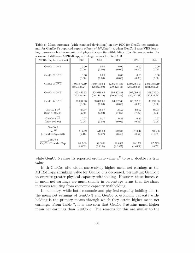
Table 6: Mean outcomes (with standard deviations) on day 1000 for GenCo net earnings,and for GenCo 3’s reported supply offers (aR,bR,CapRU ), when GenCo 3 uses VRE learn-ing to exercise both economic and physical capacity withholding. Results are reported fora range of different MPRMCap3 shrinkage values for GenCo 3.


GenCo 1 DNE 0.00 0.00 0.00 0.00 0.00(0.00) (0.00) (0.00) (0.00) (0.00)

GenCo 2 DNE 0.00 0.00 0.00 0.00 0.00(0.00) (0.00) (0.00) (0.00) (0.00)

GenCo 3 DNE 1,973,577.19 1,980,160.94 1,986,854.87 1,993,661.93 2,000,585.19(277,338.27) (278,227.89) (279,273.41) (280,482.08) (281,861.29)

GenCo 4 DNE 303,449.92 304,616.65 305,802.88 307,009.16 308,236.04(50,027.46) (50,186.55) (50,372.87) (50,587.68) (50,832.28)

GenCo 5 DNE 33,097.68 33,097.68 33,097.68 33,097.68 33,097.68(0.00) (0.00) (0.00) (0.00) (0.00)

GenCo 3 aR 98.57 98.57 98.57 98.57 98.57(true a=25.00) (7.82) (7.82) (7.82) (7.82) (7.82)

GenCo 3 bR 0.27 0.27 0.27 0.27 0.27(true b=0.01) (0.05) (0.05) (0.05) (0.05) (0.05)

GenCo 3

CapRU 517.62 515.23 512.85 510.47 508.08(TrueMaxCap=520) (2.13) (4.27) (6.40) (8.54) (10.67)

GenCo 3

CapRU/TrueMaxCap 99.54% 99.08% 98.63% 98.17% 97.71%(0.41%) (0.82%) (1.23%) (1.64%) (2.05%)

while GenCo 5 raises its reported ordinate value aR to over double its truevalue.

Both GenCos also attain successively higher mean net earnings as theMPRMCap3 shrinkage value for GenCo 3 is decreased, permitting GenCo 3to exercise greater physical capacity withholding. However, these increasesin mean net earnings are much smaller in percentage terms than the sharpincreases resulting from economic capacity withholding.

In summary, while both economic and physical capacity holding add tothe mean net earnings of GenCo 3 and GenCo 5, economic capacity with-holding is the primary means through which they attain higher mean netearnings. From Table 7, it is also seen that GenCo 3 attains much highermean net earnings than GenCo 5. The reasons for this are similar to the

36

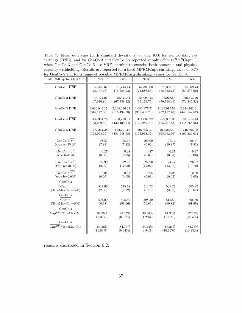
Table 7: Mean outcomes (with standard deviations) on day 1000 for GenCo daily netearnings (DNE), and for GenCo 3 and GenCo 5’s reported supply offers (aR,bRCapRU ),when GenCo 3 and GenCo 5 use VRE learning to exercise both economic and physicalcapacity withholding. Results are reported for a fixed MPRMCap5 shrinkage value of 0.70for GenCo 5 and for a range of possible MPRMCap3 shrinkage values for GenCo 3.


GenCo 1 DNE 52,462.61 51,744.44 52,380.00 62,356.15 74,969.74(75,157.13) (75,285.93) (74,686.83) (78,612.73) (80,573.60)

GenCo 2 DNE 46,174.07 45,521.31 46,099.53 55,078.56 66,413.40(67,610.86) (67,739.12) (67,179.75) (70,738.39) (72,545.32)

GenCo 3 DNE 2,030,943.15 2,068,246.24 2,083,177.71 2,139,915.52 2,244,762.61(345,177.83) (315,194.58) (339,489.78) (452,137.70) (440,142.52)

GenCo 4 DNE 402,351.76 408,758.31 411,039.92 429,387.00 461,214.44(133,209.50) (130,103.54) (130,289.40) (155,201.83) (148,768.56)

GenCo 5 DNE 192,264.38 192,291.10 192,642.57 215,248.40 246,805.08(153,958.15) (153,948.98) (153,918.35) (165,392.36) (169,829.01)

GenCo 3 aR 98.57 98.57 100.00 97.14 98.57(true a=25.00) (7.82) (7.82) (0.00) (10.87) (7.82)

GenCo 3 bR 0.27 0.28 0.27 0.27 0.27(true b=0.01) (0.05) (0.05) (0.06) (0.06) (0.06)

GenCo 5 aR 22.90 22.90 22.90 24.47 26.07(true a=10.00) (12.92) (12.92) (12.92) (13.37) (13.70)

GenCo 5 bR 0.05 0.05 0.05 0.05 0.06(true b=0.007) (0.05) (0.05) (0.05) (0.05) (0.05)

GenCo 3


GenCo 5


GenCo 3


GenCo 5


reasons discussed in Section 6.2.

37

9. Comparisons of Experimental Findings

This section summarizes the detailed experimental findings for economicand physical capacity withholding reported in Sections 6 through 8.

9.1. Comparison of Cases with One GenCo Learner

From Table 2, Table 5 and Table 6, it is seen that the relatively largeand expensive GenCo 3 (located at the load-pocket Bus 3) attains muchhigher mean net earnings relative to the benchmark no-learning case when itis able to exercise economic capacity withholding, whether or not it engagesin physical capacity withholding. Conversely, although GenCo 3’s mean netearnings increase when it exercises only physical capacity withholding, in-creasingly so for successively smaller settings for its MPRMCap3 shrinkagevalue, these gains are substantially smaller.

9.2. Comparison of Cases with Two GenCo Learners

Co-learning findings for GenCo 3 and the relatively small and inexpensiveGenCo 1 are reported in Table 3 and Figures 7-9. It is seen that GenCo 3attains much higher mean net earnings relative to the benchmark no-learningcase when using economic capacity withholding, whether or not it engages inphysical capacity withholding. Moreover, GenCo 3 has more market powerthan GenCo 1 because of its pivotal suppler status. GenCo 1 suffers a loss inmean net earnings relative to the benchmark no-learning case when GenCo 3exercises physical capacity withholding, due to network effects; and GenCo 1loses out completely (zero dispatch level) when GenCo 3 engages in eco-nomic capacity withholding. Conversely, GenCo 3 is largely unaffected bythe capacity withholding choices of GenCo 1.

Co-learning experimental findings for GenCo 3 and the relatively large butinexpensive baseload GenCo 5 are presented in Tables 4-7 and Figures 10-12.It is seen that both GenCos attain much higher mean net earnings relative tothe benchmark no-learning case when they exercise economic capacity with-holding alone or in combination with physical capacity withholding. Con-versely, GenCo 3 and GenCo 5 achieve much smaller gains in mean net earn-ings when they only exercise physical capacity withholding. Also, GenCo 3’sfavorable load-pocket location gives it more market power than GenCo 5 be-cause it is a pivotal supplier in almost every hour of every run. GenCo 5’sbest capacity withholding choices are affected by GenCo 3’s choices, but

38

GenCo 3’s best capacity withholding choices are largely unaffected by thechoices of GenCo 5.

Comparing these two co-learning experiments, it is seen that GenCo 5 isin a much better position than GenCo 1 to take advantage of the capacitywithholding choices of GenCo 3 to increase its own mean net earnings. Threefactors work against GenCo 1 here: (i) The persistent congestion on branch1-2 connecting Bus 1 to Bus 2; (ii) the location of GenCo 1 at bus 1, semi-islanded away from the load pocket Bus 3; and (iii) the relatively smallcapacity of GenCo 1.

9.3. Overall Summary of Experimental Findings

The experiments reported in this study indicate that economic capacitywithholding is much more advantageous for GenCos than physical capacitywithholding in terms of raising their mean net earnings. However, in theseexperiments the ISO does not mitigate the exercise of market power by theGenCos in any way. Effective market power mitigation requires monitoringof GenCo reported costs and capacities relative to true. It could be the casethat economic capacity withholding is more easily monitored and controlledfor than physical capacity withholding, because true operating costs can beestimated rather well from publicly available information such as fuel typeand fuel prices. Conversely, it could be more difficult to check whether forcedoutages of generation units are accurately being reported.

Finally, in all experiments reported in this study, the inexpensive butsmall GenCo 1 located at Bus 1 is persistently non-marginal. Consequently,its capacity withholding actions have little effect on the mean net earnings ofother GenCos. Conversely, when the relatively big GenCos 3 and 5 exercisecapacity withholding, GenCo 1 can either win or lose. Specifically, relative tothe benchmark no-learning case, GenCo 1: (a) loses big (zero dispatch) wheneither GenCo 3 alone engages in economic capacity withholding, GenCo 3and GenCo 1 both engage in economic capacity withholding, or GenCo 3engages in combined economic and physical capacity withholding; (b) losesmodestly when GenCo 3 alone engages in physical capacity withholding; and(c) gains big when GenCo 3 and GenCo 5 both engage in economic capacitywithholding, with or without physical capacity withholding.

The key for GenCo 1 is the economic capacity withholding of GenCo 5located at the neighboring Bus 5. If GenCo 5 aggressively reports higher-than-true marginal costs, GenCo 1 can appear to be the cheaper GenCo. Inthis case GenCo 1 is dispatched to full capacity in advance of GenCo 5 and

39

thus manages to sell its generation at the very high price determined by thereported supply offers of the marginal GenCos 3 and/or 5.

10. Concluding Remarks

The wholesale electric power market experiments conducted in this studyprovide relatively simple but empirically relevant test cases for examiningclaims about weak emergence, both positive and negative.

One issued noted by Bedau (1997) is whether weak emergence has anypractical usefulness. The co-learning patterns stressed in this study — cor-related GenCo supply offer behaviors and correlated GenCo net earningsoutcomes – are weakly emergent in the sense of Bedau (1997). These co-learning patterns could provide useful information for real-world operatorsand regulators interested in understanding the myriad complicated ways inwhich market power can be directly and indirectly exercised in wholesaleelectric power markets.

For example, they reveal the existence of complementarity effects in whichcapacity withholding exercised by a relatively large and favorably locatedGenCo, such as GenCo 3, induces capacity withholding by other relativelylarge GenCos, such as GenCo 5. The resulting impacts on the net earnings ofsmaller GenCos, such as GenCo 1, can then be positive (a complementarityeffect) or negative (a substitution effect) depending on how aggressively thelarger GenCos exercise capacity withholding and the extent to which thiswithholding results in branch congestion affecting power flow on the grid.

Another issue noted by Bedau (1997) is predictability. By definition, theweakly emergent macrostates of a system S are fully determined given themicrodynamics of S together with all impinging external conditions, includ-ing initial conditions. In what sense, then, are simulations really needed tounderstand these macrostates?

The 5-bus test cases computationally implemented in this study are de-terministic systems. By construction, the co-learning patterns that emergeduring the implementation for any one of these systems are entirely deter-mined by the specification of the initial system microstate. This specificationincludes: the methods and attributes of the GenCos, the LSEs, and the ISO(decision-making agents); the methods and attributes of the day-ahead mar-ket (institutional agent); the methods and attributes of the transmissiongrid (physical agent); and initial seed values for all pseudo-random numbergenerators included among these agents’ methods.

40

The co-learning patterns arising in these test case implementations are“explained” ex post in this study by close examination of the underlyingtransmission grid configuration, market rules, GenCo true cost and capacityattributes, and GenCo learning capabilities that appear to advantage someGenCos over others. In addition, some use is made of synchronic explanation,i.e., current co-learning patterns are “explained” in terms of the current(synchronic) interactions among the rivalrous co-learning GenCos.

However, the actual causal linkages between the initial system microstatesand the resulting co-learning patterns in these 5-bus test cases are so exceed-ingly complex it appears impossible that anyone could succeed in accuratelypredicting them in advance of experimentation. Moreover, the intensive na-ture of the experiments that would be needed to understand these linkageswith confidence is daunting; the experiments conducted in the current studyare suggestive but by no means definitive.

The saving grace here is that the 5-bus test cases, while highly simplified,capture important features of real-world wholesale electric power systems.As detailed in Weidlich and Veit (2008), agent-based researchers around theworld are building empirically-grounded testbeds for the study of such sys-tems, sharing the computational burden and speeding the real-world benefits.It seems likely that the concept of weakly emergent patterns will play an in-creasingly important role in conveying our hard-won understanding of theseand other complex real-world systems critical for both social welfare andnational security.

APPENDICES: TECHNICAL MATERIALS

A. GenCo Cost and Net Earnings Functions: Technical Details

For each day D, the supply offer sRi chosen by GenCo i to report to theISO for use in each hour H of the day-ahead market for day D+1 consists ofa linear reported marginal cost function

MCRi (pGi) = aRi + 2bRi · pGi ($/MWh) (1)

defined over a reported generation capacity interval

0 ≤ pGi ≤ CapRUi (MW ) (2)

for the generation of real power pGi. The expression MCRi (pGi) in (1) denotes

GenCo i’s reported sale reservation value for energy evaluated at pGi, i.e.,

41

the minimum dollar amount it reports it is willing to accept per MWh. Thereported marginal cost functions (1) must lie either on or above GenCo i’strue marginal cost function

MCi(pGi) = ai + 2bi · pGi ($/MWh) , (3)

where ai > 0 and bi > 0. Also, GenCo i’s reported maximum generationcapacity CapRUi in (2) must lie within its true generation capacity interval:

0 ≤ CapRUi ≤ CapUi (MW ) , (4)

where CapUi > 0.Thus, for the study at hand, a reported supply offer sRi for any GenCo i

takes the form of a reported marginal cost function (1) that can be summa-rized by a vector (aRi ,bRi ) determining its ordinate aRi and slope 2bRi , togetherwith a reported value CapRUi for its maximum generation capacity. Hence-forth such supply offers will be abbreviated in the form sRi = (aRi ,bRi ,CapRUi ).

At the beginning of any planning period, a GenCo’s avoidable costs con-sist of the operational costs that it can avoid by shutting down productiontogether with the portion of its fixed (non-operational) costs that it can avoidby taking appropriate additional actions such as asset re-use or re-sale. Inorder for production to proceed, revenues from production should at leastcover avoidable costs. In the present study the GenCos do not incur start-up/shut-down or no-load costs, and all of their fixed costs are assumed to besunk , i.e., non-avoidable. Consequently, the avoidable cost function Ca

i (pGi)for each GenCo i for any hour H is given by the integral of its true hourlymarginal cost function:

Cai (pGi) =

∫ pGi

0

MCi(p)dp = aipGi + bi[pGi]2 ($/h) (5)

where pGi lies between 0 and CapUi .Suppose GenCo i, located at bus k(i), is dispatched at level pGi(H,D) at

price LMPk(i)(H,D) for hour H of the day-ahead market for day D+1. Therevenues due to GenCo i for all 24 hours of day D+1, settled at the end ofday D, are

Revi(D) =23∑

H=00

LMPk(i)(H,D) · pGi(H,D) ($) (6)

42

Net earnings are defined as revenues minus avoidable costs. Let the avoidablecosts incurred by GenCo i on day D for any hour H of day D+1 based on itsday-D dispatch pGi(H,D) be denoted by Ca

i (H,D). Then the net earnings ofGenCo i for all 24 hours of day D+1, realized on day D, are

NEi(D) = Revi(D)−23∑

H=00

Cai (H,D) ($) (7)

Finally, as will be seen in Section C, we make use of estimates MaxDNEi

for each GenCo i’s maximum possible daily net earnings derived from itsaction domain ADi assuming “competitive” marginal-cost pricing (sales price= reported marginal cost). Specifically,

MaxDNEi = 24h ∗(

maxsRi ∈ADi

[HNE(sRi )

])($), (8)

where the hourly net earnings function HNE(sRi ) ($/h) is given by

HNE(sRi ) = [MCRi (CapRUi ) ∗ CapRUi ]− Ca

i (CapRUi ) . (9)

Note that MaxDNEi > 0 if struei ≡ (ai,bi,CapUi ) is included in GenCo i’s

action domain ADi, a requirement imposed in the following subsection.

B. GenCo Learning: Technical Details

GenCo learning is implemented using a variant of a stochastic reinforce-ment learning method developed by Roth and Erev (1995) based on human-subject experiments, hereafter referred to as the Variant Roth-Erev (VRE)learning method . The essential idea of stochastic reinforcement learning isthat the probability of choosing an action should be increased (reinforced) ifthe corresponding reward is relatively good and decreased if the correspond-ing reward is relatively poor.

Each GenCo i has available an action domain ADi consisting of a finitenumber of possible reported supply offers sRi = (aRi ,bRi ,CapRUi ), hereafter re-ferred to as actions . The action domain ADi is tailored to GenCo i’s ownparticular true cost and capacity attributes as follows: (a) it only contains re-ported marginal cost functions (1) lying on or above GenCo i’s true marginalcost function (3); and (b) it contains GenCo i’s true marginal cost function

defined over GenCo i’s true generation capacity interval, i.e., it contains struei

43

≡ (ai,bi,CapUi ). However, the action domains are constructed so as to ensureequal cardinalities and similar densities across all GenCos to avoid favoringsome GenCos over others purely through action domain construction.13

The remainder of this section describes how an arbitrary GenCo i goesabout using the VRE learning method to select actions sRi from its actiondomain ADi to submit to the ISO for the day-ahead energy market on suc-cessive days D, starting from an initial day D=1. As will be seen below, theonly relevant attribute of ADi for implementation of VRE learning is that ithas finite cardinality. Consequently, letting Mi ≥ 1 denote the cardinality ofADi, it suffices to index the actions in ADi by m = 1,...,Mi.

The initial propensity of GenCo i to choose action m ∈ ADi is given byqim(1) for m = 1,...,Mi. AMES(V2.05) permits the user to set these initialpropensity levels to any real numbers. However, the assumption used in thisstudy is that GenCo i’s initial propensity levels are all set equal to somecommon value qi(1), as follows:

qim(1) = qi(1) for all actions m ∈ ADi (10)

Now consider the beginning of any day D ≥ 1, and suppose the currentpropensity of GenCo i to choose action m in ADi is given by qim(D). Thechoice probabilities that GenCo i uses to select an action for day D arethen constructed from these propensities using the following commonly usedGibbs-Boltzmann transformation:

pim(D) =exp(qim(D)/Ti)∑Mi

j=1 exp(qij(D)/Ti), m ∈ ADi (11)

In (11), Ti is a temperature parameter that affects the degree to which GenCoi makes use of propensity values in determining its choice probabilities. AsTi→∞, then pim(D)→ 1/Mi, so that in the limit GenCo i pays no attentionto propensity values in forming its choice probabilities. On the other hand,as Ti → 0, the choice probabilities (11) become increasingly peaked over theparticular actions m having the highest propensity values qim(D), therebyincreasing the probability that these actions will be chosen.

At the end of day D, the current propensity qim(D) that GenCo i asso-ciates with each action m in ADi is updated in accordance with the following

13A complete technical explanation of this important action domain construction canbe found in Appendix B of Li et al. (2009).

44

rule. Let m′ denote the action actually selected and reported into the day-ahead market by GenCo i in day D. Also, let NEim′(D) denote the actualdaily net earnings (7) attained by GenCo i at the end of day D as its settle-ment payment for all 24 hours of the day-ahead market for day D+1. Then,for each action m in ADi,

qim(D + 1) = [1− ri]qim(D) + Responseim(D) , (12)

Responseim(D) =

[1− ei] ·NEim′(D) if m = m′

ei · qim(D)/[Mi − 1] if m 6= m′,(13)

where14 ri ∈ [0, 1], ei ∈ [0, 1), and m 6= m′ implies Mi ≥ 2. The introductionof the recency parameter ri in (12) acts as a damper on the growth of thepropensities over time. The experimentation parameter ei in (13) permitsreinforcement to spill over to some extent from a chosen action to otheractions to encourage continued experimentation with various actions in theearly stages of the learning process.

C. Calibration of GenCo Learning: Technical Details

This appendix section provides technical details in support of the dis-cussion in Section 5 regarding the sweet-spot calibration of VRE learningparameters for each learning GenCo.

C.1. Learning Calibration for Pure Economic Capacity Withholding Experi-ments

In the pure economic capacity withholding experiments reported in Sec-tion 6, each learning GenCo i makes daily use of the VRE learning methodto adjust the ordinate and slope parameters aRi ,bRi of its reported marginal

14In the original Roth-Erev method, the term qim(D) in (13) is instead given byNEim′(D). However, as explained in Nicolaisen et al. (2001), in this case there is noupdating of propensities when net earnings outcomes are zero, e.g., due to a failure to bedispatched. This can result in prolonged mushing around in the early stages of learningwhen GenCos are trying to learn appropriate supply offers, with subsequent losses of netearnings and reductions in market efficiency. The substitution of qim(D) for NEim′(D) inequation (13), introduced in Nicolaisen et al. (2001) to avoid this zero-updating problem,resulted in dramatic improvements in both GenCo net earnings and in market efficiency.

45

cost function (1) in pursuit of increased net earnings. The action domainADi for each learning GenCo i includes 100 possible reported supply offersof the form sRi = (aRi ,bRi ,CapUi ), constructed by crossing 10 distinct valuesfor aRi with ten distinct values for bRi .

The VRE recency and experimentation learning parameters ri and ei foreach learning GenCo i are fixed at common levels r = 0.04 and e = 0.96.These values for ri and ei have yielded relatively high mean net earnings forthe GenCos in intensive sensitivity experiments conducted by ISU researchersfor a variety of market contexts with VRE-learning traders, including 3-busand 5-bus wholesale power market experiments with pure economic capacityholding conditional on various settings for the initial propensity levels qi(1)and temperature levels Ti for each GenCo i [cf. Pentapalli (2008)].

Given these sweet-spot values for ri and ei, we then conducted intensiveparameter sweeps to determine sweet-spot settings for qi(1) and Ti for eachGenCo i for the 5-bus test case with each GenCo able to learn to exercise pureeconomic capacity withholding. More precisely, we systematically tested arange of positive values for αi and βi, defined as follows:

• αi = qi(1)/MaxDNEi, where qi(1) is the initial propensity level forGenCo i appearing in (10), a measure of GenCo i’s net earnings as-pirations at the beginning of the initial day 1, and MaxDNEi denotesGenCo i’s (positive) estimated maximum possible daily net earnings asdetermined in (8);

• βi = qi(1)/Ti, where Ti is the temperature parameter for GenCo iappearing in (11).

As detailed in Appendix A, the (positive) estimate MaxDNEi is exogenouslydetermined from the structural aspects of GenCo i’s action domain ADi.Consequently, any specification of positive αi and βi values for GenCo idetermines unique positive qi(1) and Ti values for GenCo i.15

Figure 4 depicts experimental findings for mean total GenCo daily netearnings attained for the 5-bus case with pure economic capacity holding

15In our earlier study Li et al. (2008), identical initial propensity and temperaturelevels were set for all learning GenCos: namely, q(1) = 6000 and T = 1000. This wasunsatisfactory since the “prior anticipated net earnings” q(1) were then set commonlyacross GenCos with different costs and locations without regard for their different netearnings opportunities.

46

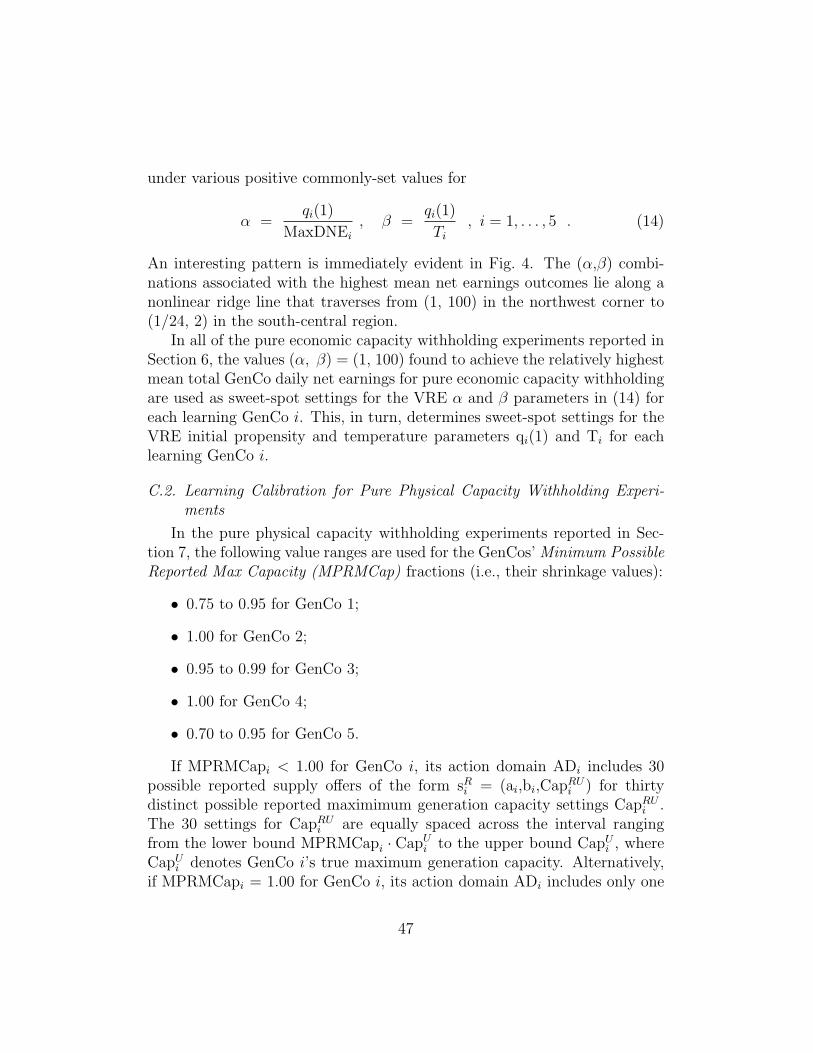
under various positive commonly-set values for

α =qi(1)

MaxDNEi

, β =qi(1)

Ti, i = 1, . . . , 5 . (14)

An interesting pattern is immediately evident in Fig. 4. The (α,β) combi-nations associated with the highest mean net earnings outcomes lie along anonlinear ridge line that traverses from (1, 100) in the northwest corner to(1/24, 2) in the south-central region.

In all of the pure economic capacity withholding experiments reported inSection 6, the values (α, β) = (1, 100) found to achieve the relatively highestmean total GenCo daily net earnings for pure economic capacity withholdingare used as sweet-spot settings for the VRE α and β parameters in (14) foreach learning GenCo i. This, in turn, determines sweet-spot settings for theVRE initial propensity and temperature parameters qi(1) and Ti for eachlearning GenCo i.

C.2. Learning Calibration for Pure Physical Capacity Withholding Experi-ments

In the pure physical capacity withholding experiments reported in Sec-tion 7, the following value ranges are used for the GenCos’ Minimum PossibleReported Max Capacity (MPRMCap) fractions (i.e., their shrinkage values):

• 0.75 to 0.95 for GenCo 1;

• 1.00 for GenCo 2;

• 0.95 to 0.99 for GenCo 3;

• 1.00 for GenCo 4;

• 0.70 to 0.95 for GenCo 5.

If MPRMCapi < 1.00 for GenCo i, its action domain ADi includes 30possible reported supply offers of the form sRi = (ai,bi,CapRUi ) for thirtydistinct possible reported maximimum generation capacity settings CapRUi .The 30 settings for CapRUi are equally spaced across the interval rangingfrom the lower bound MPRMCapi · CapUi to the upper bound CapUi , whereCapUi denotes GenCo i’s true maximum generation capacity. Alternatively,if MPRMCapi = 1.00 for GenCo i, its action domain ADi includes only one

47

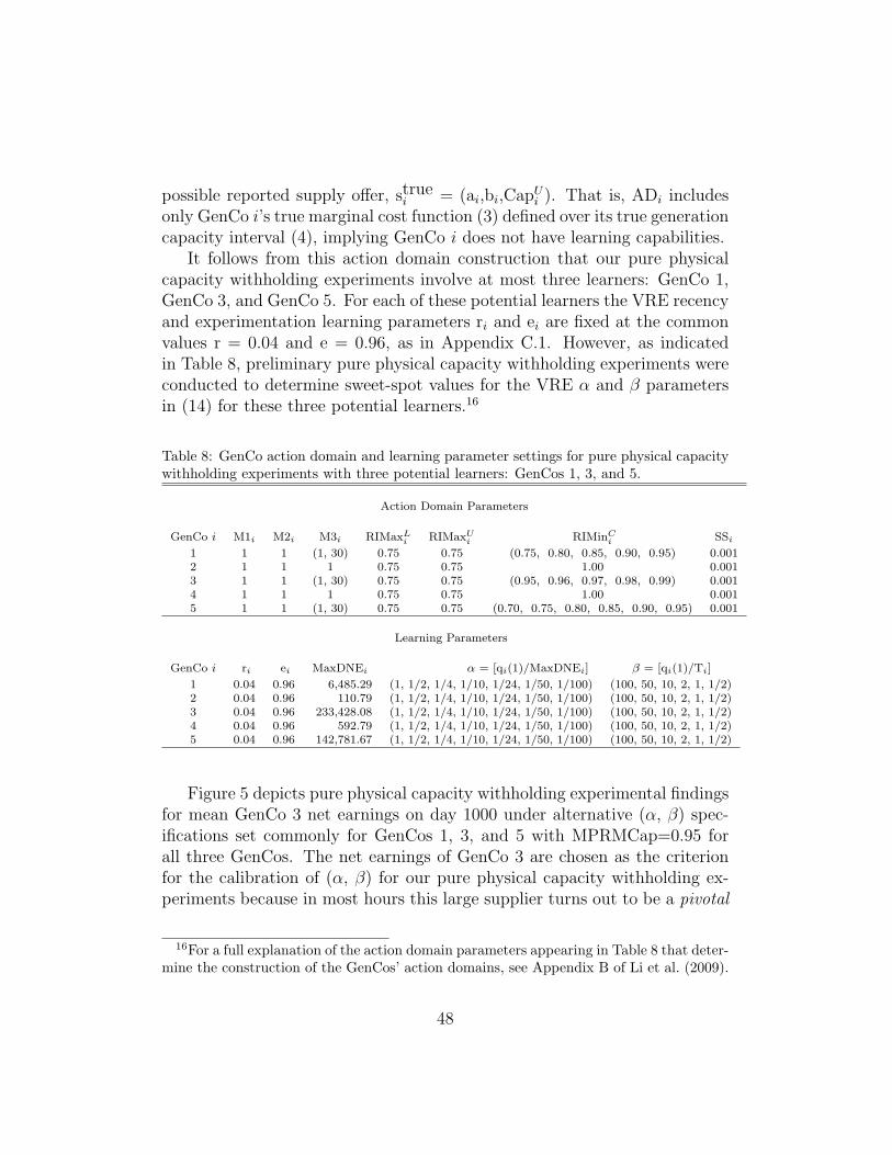
possible reported supply offer, struei = (ai,bi,CapUi ). That is, ADi includes

only GenCo i’s true marginal cost function (3) defined over its true generationcapacity interval (4), implying GenCo i does not have learning capabilities.

It follows from this action domain construction that our pure physicalcapacity withholding experiments involve at most three learners: GenCo 1,GenCo 3, and GenCo 5. For each of these potential learners the VRE recencyand experimentation learning parameters ri and ei are fixed at the commonvalues r = 0.04 and e = 0.96, as in Appendix C.1. However, as indicatedin Table 8, preliminary pure physical capacity withholding experiments wereconducted to determine sweet-spot values for the VRE α and β parametersin (14) for these three potential learners.16

Table 8: GenCo action domain and learning parameter settings for pure physical capacitywithholding experiments with three potential learners: GenCos 1, 3, and 5.

Action Domain Parameters

GenCo i M1i M2i M3i RIMaxLi RIMaxU

i RIMinCi SSi

1 1 1 (1, 30) 0.75 0.75 (0.75, 0.80, 0.85, 0.90, 0.95) 0.0012 1 1 1 0.75 0.75 1.00 0.0013 1 1 (1, 30) 0.75 0.75 (0.95, 0.96, 0.97, 0.98, 0.99) 0.0014 1 1 1 0.75 0.75 1.00 0.0015 1 1 (1, 30) 0.75 0.75 (0.70, 0.75, 0.80, 0.85, 0.90, 0.95) 0.001

Learning Parameters

GenCo i ri ei MaxDNEi α = [qi(1)/MaxDNEi] β = [qi(1)/Ti]

1 0.04 0.96 6,485.29 (1, 1/2, 1/4, 1/10, 1/24, 1/50, 1/100) (100, 50, 10, 2, 1, 1/2)2 0.04 0.96 110.79 (1, 1/2, 1/4, 1/10, 1/24, 1/50, 1/100) (100, 50, 10, 2, 1, 1/2)3 0.04 0.96 233,428.08 (1, 1/2, 1/4, 1/10, 1/24, 1/50, 1/100) (100, 50, 10, 2, 1, 1/2)4 0.04 0.96 592.79 (1, 1/2, 1/4, 1/10, 1/24, 1/50, 1/100) (100, 50, 10, 2, 1, 1/2)5 0.04 0.96 142,781.67 (1, 1/2, 1/4, 1/10, 1/24, 1/50, 1/100) (100, 50, 10, 2, 1, 1/2)

Figure 5 depicts pure physical capacity withholding experimental findingsfor mean GenCo 3 net earnings on day 1000 under alternative (α, β) spec-ifications set commonly for GenCos 1, 3, and 5 with MPRMCap=0.95 forall three GenCos. The net earnings of GenCo 3 are chosen as the criterionfor the calibration of (α, β) for our pure physical capacity withholding ex-periments because in most hours this large supplier turns out to be a pivotal

16For a full explanation of the action domain parameters appearing in Table 8 that deter-mine the construction of the GenCos’ action domains, see Appendix B of Li et al. (2009).

48

supplier, i.e., its generation capacity is essential for meeting fixed demand.In all of the pure physical capacity withholding experiments reported

in Section 7, the values (α, β) = (1/24, 100) found above to achieve therelatively highest mean daily net earnings for GenCo 3 are used as sweet-spotsettings for the VRE α and β parameters in (14) for each learning GenCo i.This, in turn, determines sweet-spot settings for the VRE initial propensityand temperature parameters qi(1) and Ti for each learning GenCo i.

C.3. Learning Calibration for Combined Capacity Withholding Experiments

In the combined economic and physical capacity withholding experimentsreported in Section 8, only two types of learning are considered. EitherGenCo 3 is the only learning GenCo (capable of both economic and phys-ical capacity withholding), or GenCo 3 and GenCo 5 are the only learningGenCos (each capable of both economic and physical capacity withholding).Consequently, the action domains ADi are constructed as follows.

The action domain AD3 for GenCo 3, always a learner, includes 3000 =10×10×30 possible reported supply offers of the form sR3 = (aR3 ,bR3 ,CapRU3 ).This action domain is constructed as the cross-product of ten values for thereported ordinate parameter aR3 , ten values for the reported slope parameterbR3 , and 30 values for the reported maximum generation capacity CapRU3 . Thereported ordinate/slope values for GenCo 3 are the same as used for GenCo3 in the pure economic withholding experiments (see Appendix C.1) and thereported maximum generation capacity values for GenCo 3 are the same asused for GenCo 3 in the pure physical capacity withholding experiments (seeAppendix C.2).

The action domain AD5 for GenCo 5 in experiments for which GenCo 5 isa learner (hence MPRMCap5 < 1.00) includes 3000 possible reported supplyoffers, constructed similarly to AD3. The action domain ADi for each non-learning GenCo i consists of only one possible reported supply offer, strue

i =(ai, bi, CapUi ). That is, ADi consists of GenCo i’s true marginal cost function(3) defined over its true generating capacity interval (4).

For each combined economic and physical capacity withholding experi-ment, the VRE learning parameters (r, e, α β) are set commonly across alllearning GenCos at the particular values (0.04, 0.96, 1, 100) determined inAppendix C.1. Ideally, a separate calibration exercise for these four VRElearning parameters should be undertaken for the combined case to see howthe sweet-spot region for the combined case geometrically relates to the

49

sweet-spot regions for each of the pure cases; this is a topic for future re-search.

Acknowledgement: The authors are grateful for exceptionally constructiveand helpful comments received from the editors and two anonymous referees.This work was supported in part by a grant from the Electric Power ResearchCenter.

References

Anderson, P.W., 1972. More is different. Science 177(4047), 393–396.

Auyang, S., 1998. Foundations of Complex-System Theories in Economics,Evolutionary Biology, and Statistical Physics. Cambridge, UK: CambridgeUniversity Press.

Baldick, R., Hogan, W., 2002. Capacity constrained supply function equilib-rium models of electricity markets: Stability, non-decreasing constraints, andfunction space iterations. University of California Energy Institute PWP-089. Online: Accessible at www.ucei.berkeley.edu/ucei/PDF/pwp089.pdf

Bedau, M., 1997. Weak emergence. In: Tomberlin, J. (Ed.), PhilosophicalPerspectives: Mind, Causation, and World. Vol. 11, Malden, MA: Blackwell,375–399.

Branner, B., 1989. The Mandelbrot set. In: Devaney, R.L., Keen, L.(Eds.). Chaos and Fractals: The Mathematics Behind the Computer Graph-ics. Proceedings of Symposia in Applied Mathematics, Vol. 39, Providence,RI: American Mathematical Society, 75-105.

Borrill, P., Tesfatsion, L., 2011. Agent-based modeling: The right mathe-matics for the social sciences? In: Davis, J.B, Hands, D. W., (Eds.). ElgarRecent Economic Methodology Companion, Northhampton, MA: EdwardElgar Publishing.

Bulow, J., Geanakoplos, J.D., and Klemperer, P., 1985. Multimarket oligopoly:Strategic substitutes and complements. Journal of Political Economy 93,488–511.

Corning, P.A., 2002. The re-emergence of “emergence”: A venerable conceptin search of a theory. Complexity 7(6), 18–30.

Dechenaux, E., Kovenock, D., 2007. Tacit Collusion and capacity withhold-ing in repeated uniform price auctions. RAND Journal of Economics 38(4),1044-1069.

50

Delgado, J., 2002. Emergence of social conventions in complex networks.Artificial Intelligence 141, 171–185.

Dessalles J.L., Ferber J., Phan D., 2008. Emergence in agent-based com-putational social science: Conceptual, formal and diagrammatic analysis.In: Yang, A., Shan, Y. (Eds.), Intelligent Complex Adaptive Systems, IdeaGroup Incorporated (IGI) Global, Chapter 9, 255–299. Online: Accessibleat www.gemas.msh-paris.fr/dphan/papers/DessallesFerberPhan2007.pdf

Devaney, R.L., Keen, L. (Eds.), 1989. Chaos and Fractals: The Mathemat-ics Behind the Computer Graphics. Proceedings of Symposia in AppliedMathematics, Vol. 39, Providence, RI: American Mathematical Society.

Gilbert, N., 1995. Emergence in social simulations. In: Gilbert, N., Conte,R. (Eds.). Artificial Societies: The Computer Simulation of Social Life.London: UCL Press, 144-156.

Gode, D.K., Sunder, S., 1993. Allocative efficiency of markets with zerointelligence traders: Market as a partical substitute for individual rationality.Journal of Political Economy 101, 119–137.

Gode, D.K., Sunder, S., 1997. What makes markets allocationally efficient?.Quarterly Journal of Economics 112(2), 603–630.

Harper, D.A., Endres, A.M., 2010. The anatomy of emergence, with a focuson capital formation. Working Paper, Department of Economics, New YorkUniversity, April.

Hayek, F.A., 1948. Individualism and Economic Order. Chicago, IL: Uni-versity of Chicago Press.

Hodgson, G.M., 2000. The concept of emergence in social science: Its historyand importance. Emergence 2(4), 65–77.

IEEE, 2011. Task Force on Open Source Software for Power Systems, Insti-tute of Electrical and Electronic Engineers. Online: Accessible atewh.ieee.org/cmte/psace/CAMS taskforce/index.htm

Kirman, A., 1993. Ants, rationality, and recruitment. Quarterly Journal ofEconomics 108(1), 137-156.

Kittock, J.E., 1995. Emergent conventions and the structure of multi-agentsystems. In: Nadel, L., Stein, D. (Eds.), 1993 Lectures in Complex Sys-tems, SFI Studies in the Sciences of Complexity, Vol. VI, Santa Fe Institute,Addison-Wesley, Reading, MA, 507–521.

51

Kuperberg, M., 2006. The two faces of emergence in economics. Presented atEmergent Systems: A Discussion, Center for Science in Society, Bryn MawrCollege, July 18. Online: Accessible atwww.econ.iastate.edu/tesfatsi/TwoFacesOfEmergence.MKuperberg.pdf

Lally, J., 2002. Financial transmission rights: Auction example, Section 6 inFinancial Transmission Rights Draft 01-10-02, m-06 ed., ISO New England,Inc.

Laughlin, R.B., Pines, D., Schmalian, J., Stojkovic, B.P., Wolynes, P., 2000.The middle way. Proceedings of the National Academy of Sciences 97, 32–37.

Laughlin, R.B., 2002. The physical basis of computability. Computing inScience and Engineering 4(3), 27–30.

Lewis, P., 2011. Emergent properties in the work of Friedrich Hayek. Journalof Economic Behavior and Organization, to appear.

Li, H., Tesfatsion, L., 2009a. Capacity withholding in restructured wholesalepower markets: An agent-based testbed study, Proceedings of the IEEEPower Systems Conference & Exposition (PSCE), Seattle, WA. Online:www.econ.iastate.edu/tesfatsi/CapacityWithhold.LiTesPSCE2009.pdf

Li, H., Tesfatsion, L., 2009b. The AMES wholesale power market testbed: Acomputational laboratory for research, teaching, and training. Proceedings ofthe IEEE Power and Energy Society General Meeting, Calgary, Alberta, CA.Online: www.econ.iastate.edu/tesfatsi/AMESTestBed.2009IEEEPESGM.pdf

Li, H., Tesfatsion, L., 2009c. Development of open source software for powermarket research: The AMES testbed”, Journal of Energy Markets 2(2), 111–128.

Li, H., Tesfatsion, L., 2011. ISO Net Surplus Collection and Allocation inWholesale Power Markets under LMP. IEEE Transactions on Power Systems26(2), 627–641.

Li, H., Sun, J., Tesfation, L., 2008. Dynamic LMP response under alternativeprice-cap and price-sensitive demand scenarios. Proceedings of the IEEEPower and Energy Society General Meeting, Pittsburgh, PA.

Li, H., Sun, J., Tesfatsion, L., 2009. Separation and volatility of locationalmarginal prices in restructured wholesale power markets. Economics Work-ing Paper #09009, Iowa State University, Ames, Iowa. Online: Accessible atwww.econ.iastate.edu/research/publications/viewabstract.asp?pid=13075

52

Nicolaisen, J., Petrov, V., Tesfatsion, L., 2001. Market power and efficiencyin a computational electricity market with discriminatory double-auctionpricing. IEEE Transactions on Evolutionary Computation 5(5), 504–523.

O’Connor, R., Wong, H.Y., 2006. Emergent properties. In: Zalta, E.N.(Ed.). The Stanford Encyclopedia of Philosophy. Online: Accessible athttp://plato.stanford.edu/entries/properties-emergent/

Pentapalli, M., 2008. A comparative study of Roth-Erev and modified Roth-Erev reinforcement learning algorithms for uniform-price double auctions.M.S. Thesis, Computer Science Department, Iowa State University, Ames,Iowa.

Roth, A.E., Erev, I., 1995. Learning in extensive form games: Experimen-tal data and simple dynamic models in the intermediate term. Games andEconomic Behavior 8, 164–212.

Schelling, T.S., 1978. Micromotives and Macrobehavior. New York, NY:W.W. Norton & Co.

Shahidehpour, M., Yamin, H., Li, Z., 2002. Market Operations in ElectricPower Systems. New York:IEEE/Wiley-Interscience.

Shoham, Y., Tennenholtz, M., 1994. Co-learning and the evolution of socialactivity. Technical Report. Stanford University.

Smith, A., 1937. An Inquiry into the Nature and Causes of the Wealth ofNations. New York, NY: Cannan Edition, American Modern Library Series.

Squazzoni, F. (Ed.), 2006. Epistemological Aspects of Computer Simulationin the Social Sciences. Lecture Notes in Artificial Intelligence, Vol. 5466,Springer-Verlag Berlin, Heidelberg.

Stephan, A., 1999. Varieties of emergentism. Evolution and Cognition 5(1),49–59.

Tellidou, A., Bakirtzis, A., 2007. Agent-based analysis of capacity withhold-ing and tacit collusion in electricity markets. IEEE Transactions on PowerSystems 22(4), 1735–1742.

Tesfatsion, L., 2010. AMES Wholesale Power Market Testbed Homepage,Iowa State University. Online: Accessible atwww.econ.iastate.edu/tesfatsi/AMESMarketHome.htm

53

Tesfatsion, L., Judd, K.L., 2006. Handbook of Computational Economics,Volume 2: Agent-Based Computational Economics. Handbooks in Eco-nomics Series. Amsterdam:North-Holland, 831–880.

Tirole, J., 2003. The Theory of Industrial Organization. Fourteenth Printing.Cambridge, MA: MIT Press.

Urbano, P., Balso, J., Antunes, L., Moniz, L., 2009. Force versus majority: Acomparison in convention emergence efficiency. In: Hubner, J., Matson, E.,Boissier, O., and Dignum, V. (Eds.), Coordination, Organizations, Institu-tions, and Norms in Agent Systems IV. Lecture Notes in Computer Science,Vol. 5428, Springer Berlin/Heidelberg, 48–63.

Weidlich, A., Veit, D., 2008. A critical survey of agent-based wholesaleelectricity market models. Energy Economics 30(4), 1728–1759.

54

Documents

Co-Learning Patterns As Emergent Market Phenomena: An