CO2 Capture by Absorption with Potassium Carbonate

Third Quarterly Report 2006

Quarterly Progress Report

Reporting Period Start Date: July 1, 2006 Reporting Period End Date: September 30, 2006

Authors: Gary T. Rochelle, Eric Chen, Babatunde Oyenekan, Andrew Sexton, Jason Davis, Marcus Hilliard, Amornvadee Veawab

October 25, 2006 DOE Award #: DE-FC26-02NT41440 Department of Chemical Engineering

The University of Texas at Austin

2

Disclaimer This report was prepared as an account of work sponsored by an agency of the United States Government. Neither the United States Government nor any agency thereof, nor any of their employees, makes any warranty, express or implied, or assumes any legal liability or responsibility for the accuracy, completeness, or usefulness of any information, apparatus, product, or process disclosed, or represents that its use would not infringe privately owned rights. Reference herein to any specific commercial product, process, or service by trade name, trademark, manufacturer, or otherwise does not necessarily constitute or imply its endorsement, recommendation, or favoring by the United States Government or any agency thereof. The views and opinions of authors expressed herein do not necessarily state or reflect those of the United States Government or any agency thereof.

3

Abstract The objective of this work is to improve the process for CO2 capture by alkanolamine absorption/stripping by developing an alternative solvent, aqueous K2CO3 promoted by piperazine. Ethylenediamine was detected in a degraded solution of MEA/PZ solution, suggesting that piperazine is subject to oxidation. Stripper modeling has demonstrated that vacuum strippers will be more energy efficient if constructed short and fat rather than tall and skinny. The matrix stripper has been identified as a configuration that will significantly reduce energy use. Extensive measurements of CO2 solubility in 7 m MEA at 40 and 60oC have confirmed the work by Jou and Mather. Corrosion of carbon steel without inhibitors increases from 19 to 181 mpy in lean solutions of 6.2 m MEA/PZ as piperazine increases from 0 to 3.1 m.

4

Contents

Disclaimer ........................................................................................................................................2 Abstract ............................................................................................................................................3 List of Figures ..................................................................................................................................6 List of Tables ...................................................................................................................................8 Introduction......................................................................................................................................9 Experimental ....................................................................................................................................9 Results and Discussion ....................................................................................................................9 Conclusions....................................................................................................................................10 Future Work ...................................................................................................................................11 Task 1 – Modeling Performance of Absorption/Stripping of CO2 with Aqueous K2CO3 Promoted

by Piperazine......................................................................................................................12 Subtask 1.3 – Absorber Model...........................................................................................12

Introduction........................................................................................................... 12 Experimental ......................................................................................................... 12 Conclusion and Future Work ................................................................................ 18

Subtask 1.3b – Rate-based Modeling – Aspen Custom Modeler for Stripper...................19 Introduction........................................................................................................... 19 Experimental (Model Formulation) ...................................................................... 19 Results and Discussion ......................................................................................... 24 Conclusions and Future Work .............................................................................. 25

Subtask 1.8a – Alternative stripper configurations – Aspen Custom Modeler for Stripper26 Introduction........................................................................................................... 26 Experimental (Model Formulation) ...................................................................... 27 Results and Discussion ......................................................................................... 27 Conclusions........................................................................................................... 31 References............................................................................................................. 31

Task 3 – Solvent Losses.................................................................................................................31 Subtask 3.1 – Analysis of Degradation Products...............................................................31

Introduction........................................................................................................... 31 Experimental ......................................................................................................... 32 Results................................................................................................................... 33 Conclusions and Future Work .............................................................................. 40 References............................................................................................................. 40

Subtask 3.3 – Thermal Degradation...................................................................................41 Introduction........................................................................................................... 41 Theory ................................................................................................................... 41 Method .................................................................................................................. 42 Results and Discussion ......................................................................................... 42 Future Work .......................................................................................................... 44 References............................................................................................................. 45

Subtask 3.4 – Amine Volatility..........................................................................................45 Reagents................................................................................................................ 45 Experimental Methods .......................................................................................... 45 Results................................................................................................................... 45

5

Future work........................................................................................................... 47 Conclusions........................................................................................................... 47

Task 5 – Corrosion.........................................................................................................................47 Introduction........................................................................................................... 47 Results................................................................................................................... 48

References......................................................................................................................................54

6

List of Figures Figure 1: Aspen Flash ................................................................................................................... 12

Figure 2: Mass transfer with reaction in the boundary layer and liquid diffusion........................ 20

Figure 3: Mass transfer with equilibrium reaction........................................................................ 21

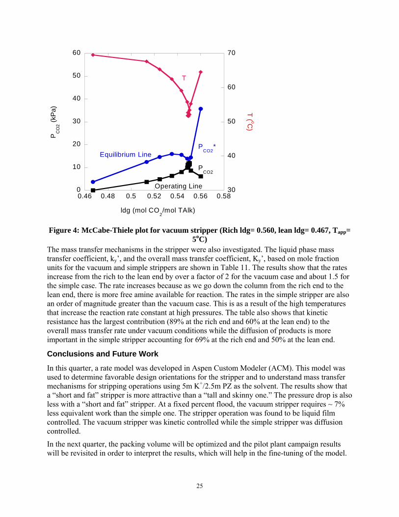
Figure 4: McCabe-Thiele plot for vacuum stripper (Rich ldg= 0.560, lean ldg= 0.467, Tapp= 5oC)....................................................................................................................................................... 25

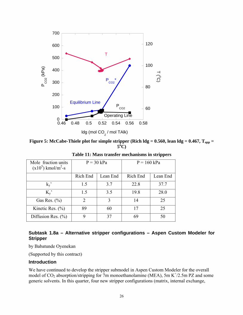
Figure 5: McCabe-Thiele plot for simple stripper (Rich ldg = 0.560, lean ldg = 0.467, Tapp = 5oC)....................................................................................................................................................... 26

Figure 6: Sample Analysis for Experiment 5/18/2006 ................................................................. 35

Figure 7: Sample Analysis for Experiment 9/27/2006 ................................................................. 35

Figure 8: Sample Analysis for Experiment 9/28/2006 ................................................................. 36

Figure 9: Sample Analysis for Experiment 6/7/2006 ................................................................... 36

Figure 10: Sample Analysis for Experiment 9/29/2006 ............................................................... 37

Figure 11: 7m MEA spiked with known thermal degradation products....................................... 43

Figure 12: GC chromatogram of MEA solution held at 150oC for 3 weeks................................. 43

Figure 13: Undegraded MEA sample injected 10 times............................................................... 44

Figure 14: Process Flow Diagram for Vapor Phase Speciation Experiments .............................. 46

Figure 15: Comparison of CO2 solubility results from this work and Jou et al. (1995) to predictions from Freguia (2002) at 40 and 60oC .......................................................................... 47

Figure 16: Cyclic polarization curves of carbon steel in 7m MEA-1.7m piperazine containing 0.20 mol/mol CO2 under 10% O2 at 40 and 80oC ......................................................................... 49

Figure 17: Effect of solution temperature on corrosion rate of carbon steel (7m MEA-1.7 m piperazine solution containing 0.20 mol/mol CO2 loading under 10% O2 in gas at 40 and 80oC)........................................................................................................................................................ 49

Figure 18: Cyclic polarization curves of carbon steel in 5m MEA-1.2 m piperazine containing 0.20 mol/mol CO2 and 1 wt% heat-stable salt at 80oC ................................................................. 50

Figure 19: Effect of heat-stable salts on corrosion rates of carbon steel in the absence of oxygen (5m MEA-1.2 m piperazine solution containing 0.20 mol/mol CO2 loading and 1 wt% heat-stable salt at 80oC)................................................................................................................................... 50

Figure 20: Cyclic polarization curves of carbon steel in 5m MEA-1.2 m piperazine containing 0.20 mol/mol CO2 loading, 10% O2 and 1 wt% heat-stable salt at 80oC...................................... 51

Figure 21: Effect of heat-stable salt on corrosion rates of carbon steel in the presence of oxygen (5m MEA-1.2 m piperazine solution containing 0.20 mol/mol CO2 loading, 10% O2 and 1 wt% heat-stable salt at 80oC) ................................................................................................................ 51

Figure 22: Cyclic polarization curves of carbon steel in aqueous solutions of MEA-PZ mixtures containing 0.20 mol/mol CO2 loading at 80oC ............................................................................. 52

7

Figure 23: Effect of piperazine concentration on corrosion rates of carbon steel (aqueous solutions of 6.2 m MEA and 6.2 m MEA-piperazine containing 0.20 mol/mol CO2 loading at 80oC). ............................................................................................................................................ 53

Figure 24: Cyclic polarization curves of carbon steel in 5m MEA-1.2 m PZ mixtures containing 0.20 mol/mol CO2 loading at 80oC with and without oxygen ...................................................... 53

Figure 25: Effect of oxygen on corrosion rates of carbon steel (5m MEA-1.2 m piperazine solution containing 0.20 mol/mol CO2 loading, 5% O2 and at 80oC) ........................................... 53

8

List of Tables Table 1: Heat of Absorption Comparison, Charge H+PZCOO- = 0.............................................. 13

Table 2: Heat of Absorption, Charge H+PZCOO- = 0.0001 ......................................................... 14

Table 3: Equilibrium Constants in the Hilliard Aspen Electrolyte NTRL Model ........................ 15

Table 4: Heats of Formation Used ................................................................................................ 15

Table 5: Heat of Absorption with Heat of Formation Adjustment ............................................... 16

Table 6: Heat Capacity Constants 2 Parameter............................................................................. 17

Table 7: Reconciled Heat of Absorption Results.......................................................................... 18

Table 8: Adjustable constants in VLE expression ........................................................................ 22

Table 9: Loadings at different equilibrium partial pressures of CO2 at 40oC............................... 22

Table 10: “Short and Fat” vs. “Tall and Skinny” Column............................................................ 24

Table 11: Mass transfer mechanisms in strippers ......................................................................... 26

Table 12: Predicted performance of different solvents using various stripper configurations ..... 29

Table 13: Energy requirement for separation and compression to 10 MPa.................................. 30

Table 14: Low Gas Flow Degradation Product Rates .................................................................. 34

Table 15: Summary of Ammonia Rates for High Gas Flow Experiments ................................... 37

Table 16: Summary of Amine/Aldehyde Concentrations............................................................. 38

Table 17: Summary of NOx and CO Concentrations .................................................................... 38

Table 18: Summary of Amine Volatility ...................................................................................... 39

9

Introduction The objective of this work is to improve the process for CO2 capture by alkanolamine absorption/stripping by developing an alternative solvent, aqueous K2CO3 promoted by piperazine. This work expands on parallel bench-scale work with system modeling and pilot plant measurements to demonstrate and quantify the solvent process concepts.

Gary Rochelle is supervising the bench-scale and modeling work; Frank Seibert has supervised the pilot plant. Three graduate students (Eric Chen, Babatunde Oyenekan, and Andrew Sexton) have received support during this quarter for direct effort on the scope of this contract. Two students supported by other funding have made contributions this quarter to the scope of this project (Marcus Hilliard, Jason Davis – Industrial Associates). Subcontract work was performed by Manjula Nainar at the University of Regina under the supervision of Amy Veawab. Experimental Subtask 1.3a describes development of a model in RateSep for the absorber.

Subtask 1.3b describes development of a rate model for the stripper in Aspen Custom Modeler.

Subtask 3.1 presents methods for analyzing amine degradation products by anion and cation chromatography.

Subtask 3.3 describes a method of gas chromatography for amine degradation products.

Subtask 3.4 describes methods for measuring amine, CO2, and water vapor pressure over loaded solutions of amine.

Task 5 describes electrochemical methods for measuring corrosion.

Results and Discussion Progress has been made on five subtasks in this quarter:

Subtask 1.3a – Absorber Model The RateSep model of the Absorber has been fixed to correctly represent the heat of CO2 absorption.

Subtask 1.3b – Stripper model The rate-based model has been used to estimate the packing height for simple strippers at normal pressure and vacuum.

Subtask 1.8a – Predict Flowsheet Options The equilibrium model has been used to evaluate energy requirements with a number of stripper configurations and solvent compositions. A paper manuscript has been prepared on this activity.

Subtask 3.1 – Analysis of Degradation Products Experiments have been performed with blends of piperazine and monoethanolamine with both low and high oxidant flowrates. Degradation products have been quantified by anion and cation chromatography.

10

Subtask 3.3 – Thermal Degradation Samples of loaded MEA were degraded at 150oC. These initial samples were analyzed by gas chromatography.

Subtask 3.4 – Amine Volatility CO2, amine, and water vapor pressures have been measured at 40 and 60oC over loaded solutions of 7 m MEA to qualify the new measurement method.

Subtask 4.1 – Sulfate Precipitation The solubility of potassium sulfate was measured in solutions of MEA and MEA/PZ.

Subtask 5.1 – Corrosion in base solution compared to MEA Electrochemical measurements of corrosion have been performed in solutions of MEA and piperazine in the absence of inhibitors.

Conclusions 1. Correct application of thermodynamics in RateSep requires entries for heat capacities and heats of formation that are consistent with the equilibrium constants used in the chemistry block.

2. Ethylenediamine was detected in a MEA/PZ solution degraded in the low gas flow apparatus. Therefore it is apparent that piperazine degrades along with MEA in this solvent.

3. A “short and fat” stripper will require less energy than a “tall and skinny” stripper without much more packing volume.

4. The stripper is controlled by liquid film resistance. A vacuum stripper is controlled by mass transfer with fast reaction. A stripper at normal pressure is controlled by diffusion of reactants and products.

5. MEA/PZ and MDEA/PZ are solvent alternatives to 7m MEA that can reduce total equivalent work for the configurations studied.

6. The performance of the alternative configurations is matrix > internal exchange > multipressure with split feed > flashing feed.

7. At a fixed capacity, solvents with high heats of absorption require less energy for stripping. This is a consequence of the temperature swing effect.

8. Less energy is required with high capacity solvents with equivalent heat of absorption.

9. The best solvent and process configuration in this study, matrix (295/160) using MDEA/PZ, offers 22% energy savings over the baseline and 15% savings over the improved baseline with stripping and compression to 10 MPa.

10. The typical predicted equivalent work requirement for stripping and compression to 10 MPa (30 kJ/gmol CO2) is about 20% of the power output from a 500 MW power plant with 90% CO2 removal.

11. Analysis of MEA degradation products by gas chromatography in a polar column is not reproducible because retained species bleed into later samples.

11

12. Extensive measurements of CO2 solubility in 7 m MEA at 40 and 60oC have confirmed the work by Jou and Mather.

13. Corrosion of carbon steel without inhibitors increases from 19 to 181 mpy in lean solutions of 6.2 m MEA/PZ as piperazine increases from 0 to 3.1 m.

14. In solutions of MEA/PZ without inhibitors, the corrosion of carbon steel increases with temperature, oxygen, and heat stable salts.

Future Work We expect the following accomplishments in the next quarter: Subtask 1.7 – Simulate and Optimize Packing Effects The absorber data from campaigns 1, 2, and 4 will be simulated with the Ratesep model. The stripper data will be simulated with the ACM model.

Subtask 3.1 – Analysis of Degradation Products One additional unknown peak from ion chromatography will be identified. Work will start on the development of a HPLC method for thermal degradation products of MEA and PZ.

Subtask 3.3 – Thermal Degradation Samples of loaded MEA and potassium carbonate/PZ will be degraded at 150ºC.

Subtask 4.1 – Sulfate Precipitation Additional measurements will be made of solubility of potassium sulfate solids in MEA solutions.

Subtask 5.4 – Effects of corrosion inhibitors Corrosion of MEA/PZ solutions will be measured with the addition of Cu++.

12

Task 1 – Modeling Performance of Absorption/Stripping of CO2 with Aqueous K2CO3 Promoted by Piperazine Subtask 1.3a – Absorber Model

by Eric Chen

(Supported by this contract)

Introduction

Hilliard (2005) developed a VLE model in Aspen Plus for the potassium carbonate/piperazine (K+/PZ) system. The model was based on the work done by Cullinane (2005) and incorporated additional experimental data obtained by Hilliard. An absorber model for CO2 absorption was developed in Aspen RateFrac using the Hilliard VLE model. The absorber model predicted a strange temperature profile, which seemed to indicate that the heats of absorption were being incorrectly predicted. An absorber model for the K+/PZ system was needed to validate several pilot plant runs and therefore the heats of absorption for the VLE model needed to be reconciled.

Experimental

Heats of Absorption Calculation

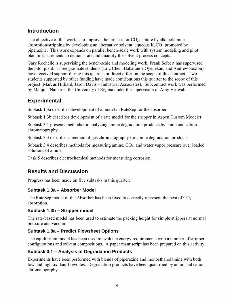
Aspen Plus flash calculations using the potassium carbonate/piperazine (K+/PZ) VLE model developed by Hilliard (2005) generated heat duty and vapor liquid equilibrium data. The flash calculation was done by absorbing a gas stream of CO2 into a liquid containing potassium carbonate, piperazine, and CO2 (Figure 1). Flash calculations were done with a vapor fraction of 1e-9 and the pressure and temperature of the inlet streams were adjusted to match the flash pressure and temperature conditions.

Figure 1: Aspen Flash

The heat duties from the Aspen Flash calculation represent the heat of absorption of CO2 into the K+/PZ solvent. The heat of absorption can also be calculated using the Clausius-Clapeyron equation from the vapor pressure data generated by the flash calculation. The

13

Clausius-Clapeyron equation assumes that the liquid molar volume is negligible relative to the vapor molar volume and that the heat of absorption is independent of temperature (Smith, et al., 1996). The Clausius-Clapeyron is given by the following equation:

⎟⎠

⎞⎜⎝

⎛ −∆

−=12,

, 11ln12

22

TTRH

PP

AB

TCO

TCO ( 1 )

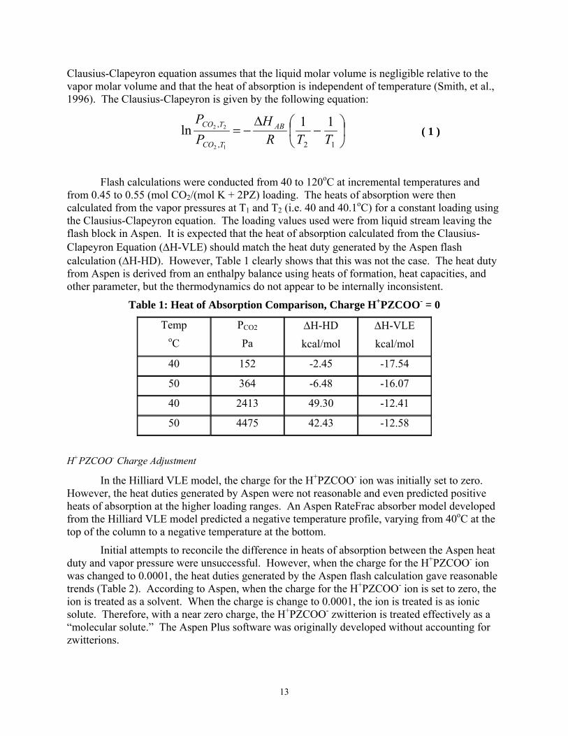
Flash calculations were conducted from 40 to 120oC at incremental temperatures and from 0.45 to 0.55 (mol CO2/(mol K + 2PZ) loading. The heats of absorption were then calculated from the vapor pressures at T1 and T2 (i.e. 40 and 40.1oC) for a constant loading using the Clausius-Clapeyron equation. The loading values used were from liquid stream leaving the flash block in Aspen. It is expected that the heat of absorption calculated from the Clausius-Clapeyron Equation (∆H-VLE) should match the heat duty generated by the Aspen flash calculation (∆H-HD). However, Table 1 clearly shows that this was not the case. The heat duty from Aspen is derived from an enthalpy balance using heats of formation, heat capacities, and other parameter, but the thermodynamics do not appear to be internally inconsistent.

Table 1: Heat of Absorption Comparison, Charge H+PZCOO- = 0

Temp oC

PCO2

Pa ∆H-HD

kcal/mol

∆H-VLE

kcal/mol

40 152 -2.45 -17.54

50 364 -6.48 -16.07

40 2413 49.30 -12.41

50 4475 42.43 -12.58

H+PZCOO- Charge Adjustment

In the Hilliard VLE model, the charge for the H+PZCOO- ion was initially set to zero. However, the heat duties generated by Aspen were not reasonable and even predicted positive heats of absorption at the higher loading ranges. An Aspen RateFrac absorber model developed from the Hilliard VLE model predicted a negative temperature profile, varying from 40oC at the top of the column to a negative temperature at the bottom.

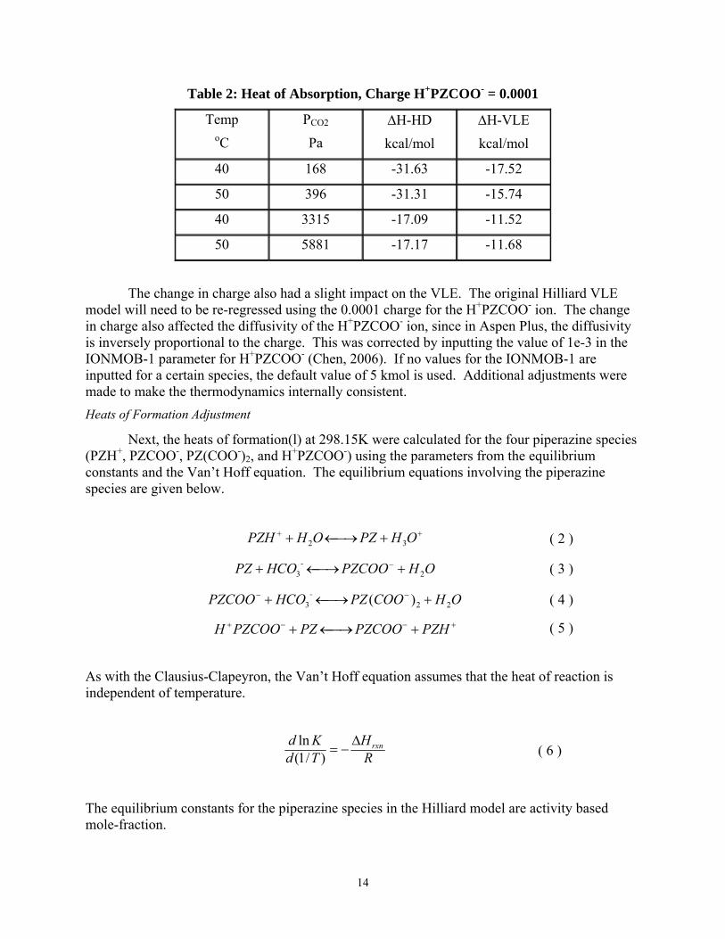
Initial attempts to reconcile the difference in heats of absorption between the Aspen heat duty and vapor pressure were unsuccessful. However, when the charge for the H+PZCOO- ion was changed to 0.0001, the heat duties generated by the Aspen flash calculation gave reasonable trends (Table 2). According to Aspen, when the charge for the H+PZCOO- ion is set to zero, the ion is treated as a solvent. When the charge is change to 0.0001, the ion is treated is as ionic solute. Therefore, with a near zero charge, the H+PZCOO- zwitterion is treated effectively as a “molecular solute.” The Aspen Plus software was originally developed without accounting for zwitterions.

14

Table 2: Heat of Absorption, Charge H+PZCOO- = 0.0001

Temp oC

PCO2

Pa ∆H-HD

kcal/mol

∆H-VLE

kcal/mol

40 168 -31.63 -17.52

50 396 -31.31 -15.74

40 3315 -17.09 -11.52

50 5881 -17.17 -11.68

The change in charge also had a slight impact on the VLE. The original Hilliard VLE model will need to be re-regressed using the 0.0001 charge for the H+PZCOO- ion. The change in charge also affected the diffusivity of the H+PZCOO- ion, since in Aspen Plus, the diffusivity is inversely proportional to the charge. This was corrected by inputting the value of 1e-3 in the IONMOB-1 parameter for H+PZCOO- (Chen, 2006). If no values for the IONMOB-1 are inputted for a certain species, the default value of 5 kmol is used. Additional adjustments were made to make the thermodynamics internally consistent. Heats of Formation Adjustment

Next, the heats of formation(l) at 298.15K were calculated for the four piperazine species (PZH+, PZCOO-, PZ(COO-)2, and H+PZCOO-) using the parameters from the equilibrium constants and the Van’t Hoff equation. The equilibrium equations involving the piperazine species are given below.

++ +⎯→←+ OHPZOHPZH 32 ( 2 )

OHPZCOOΗCΟPZ -23 +⎯→←+ − ( 3 )

OHCOOPZΗCΟPZCOO -223 )( +⎯→←+ −− ( 4 )

+−−+ +⎯→←+ PZHPZCOOPZPZCOOH ( 5 )

As with the Clausius-Clapeyron, the Van’t Hoff equation assumes that the heat of reaction is independent of temperature.

RH

TdKd rxn∆

−=)/1(ln ( 6 )

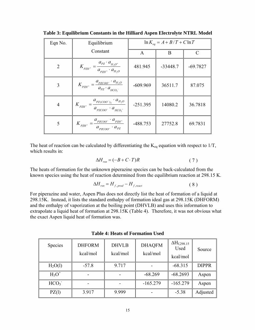
The equilibrium constants for the piperazine species in the Hilliard model are activity based mole-fraction.

15

Table 3: Equilibrium Constants in the Hilliard Aspen Electrolyte NTRL Model

TCTBAKeq ln/ln ++= Eqn No.

Equilibrium

Constant A B C

2 OHPZH

OHPZ

PZH aaaa

K2

3

⋅⋅

=+

+

+ 481.945 -33448.7 -69.7827

3 −

−

+ ⋅⋅

=3

2

HCOPZ

OHPZCOOPZH aa

aaK -609.969 36511.7 87.075

4 −−

−

+ ⋅

⋅=

3

22)(

HCOPZCOO

OHCOOPZPZH aa

aaK -251.395 14080.2 36.7818

5 PZPZCOO

PZHPZCOOPZH aa

aaK

⋅⋅

=−

+−

+ -488.753 27752.8 69.7831

The heat of reaction can be calculated by differentiating the Keq equation with respect to 1/T, which results in:

RTCBHrxn )( ⋅+−=∆ ( 7 )

The heats of formation for the unknown piperazine species can be back-calculated from the known species using the heat of reaction determined from the equilibrium reaction at 298.15 K.

reactfprodfrxn HHH ,, −=∆ ( 8 )

For piperazine and water, Aspen Plus does not directly list the heat of formation of a liquid at 298.15K. Instead, it lists the standard enthalpy of formation ideal gas at 298.15K (DHFORM) and the enthalpy of vaporization at the boiling point (DHVLB) and uses this information to extrapolate a liquid heat of formation at 298.15K (Table 4). Therefore, it was not obvious what the exact Aspen liquid heat of formation was.

Table 4: Heats of Formation Used

Species

DHFORM

kcal/mol

DHVLB

kcal/mol

DHAQFM

kcal/mol

∆Hf,298.15 Used

kcal/mol Source

H2O(l) -57.8 9.717 - -68.315 DIPPR

H3O+ - - -68.269 -68.2693 Aspen

HCO3- - - -165.279 -165.279 Aspen

PZ(l) 3.917 9.999 - -5.38 Adjusted

16

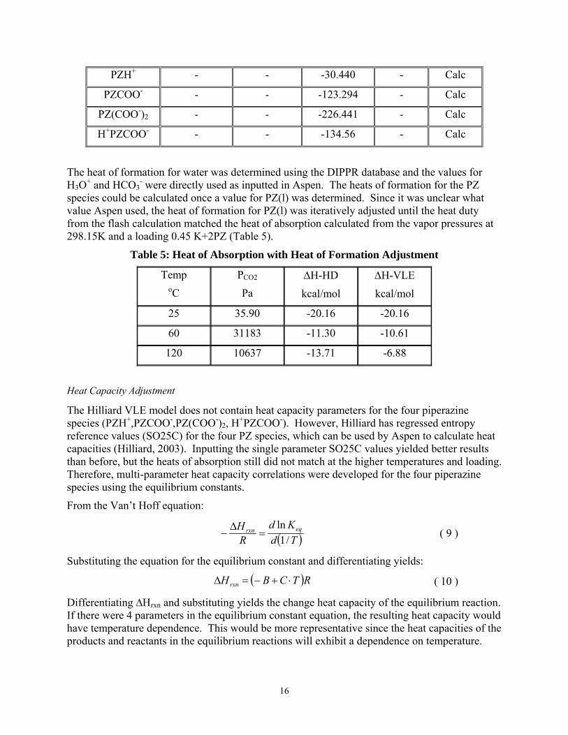
PZH+ - - -30.440 - Calc

PZCOO- - - -123.294 - Calc

PZ(COO-)2 - - -226.441 - Calc

H+PZCOO- - - -134.56 - Calc

The heat of formation for water was determined using the DIPPR database and the values for H3O+ and HCO3

- were directly used as inputted in Aspen. The heats of formation for the PZ species could be calculated once a value for PZ(l) was determined. Since it was unclear what value Aspen used, the heat of formation for PZ(l) was iteratively adjusted until the heat duty from the flash calculation matched the heat of absorption calculated from the vapor pressures at 298.15K and a loading 0.45 K+2PZ (Table 5).

Table 5: Heat of Absorption with Heat of Formation Adjustment

Temp oC

PCO2

Pa ∆H-HD

kcal/mol

∆H-VLE

kcal/mol

25 35.90 -20.16 -20.16

60 31183 -11.30 -10.61

120 10637 -13.71 -6.88

Heat Capacity Adjustment

The Hilliard VLE model does not contain heat capacity parameters for the four piperazine species (PZH+,PZCOO-,PZ(COO-)2, H+PZCOO-). However, Hilliard has regressed entropy reference values (SO25C) for the four PZ species, which can be used by Aspen to calculate heat capacities (Hilliard, 2003). Inputting the single parameter SO25C values yielded better results than before, but the heats of absorption still did not match at the higher temperatures and loading. Therefore, multi-parameter heat capacity correlations were developed for the four piperazine species using the equilibrium constants.

From the Van’t Hoff equation:

( )Td

KdRH eqrxn

/1ln

=∆

− ( 9 )

Substituting the equation for the equilibrium constant and differentiating yields:

( )RTCBHrxn ⋅+−=∆ ( 10 )

Differentiating ∆Ηrxn and substituting yields the change heat capacity of the equilibrium reaction. If there were 4 parameters in the equilibrium constant equation, the resulting heat capacity would have temperature dependence. This would be more representative since the heat capacities of the products and reactants in the equilibrium reactions will exhibit a dependence on temperature.

17

RCdT

HdC rxnrxnp ⋅=

∆=∆ , ( 11 )

Applying the same principles used to calculate the heats of formation, the heat capacities for the unknown piperazine species can be calculated.

∑ ∑−=∆ reacPprodPrxnP CCC ,,, ( 12 )

Again, as before it was not obvious from the Aspen property database what it was using to calculate the heat capacities for the individual components. First, a heater block was setup in the Aspen process flowsheet. PZ and H2O were entered individually and heated at incremental temperatures ranging from 25 to 120oC. The heat capacity was calculated from the heat input calculated by Aspen to heat the component by 0.1oC. The heater block Aspen calculated zero heat input for the HCO3

- and H3O+, which made sense because they were ions. In Aspen, under the CPAQ0-1 tab, it lists a single parameter heat capacity for H3O+ as 17.98 cal/mol-K.

In Aspen Plus, under the Prop-Set tab in Parameters, the heat capacities (CP) for the 4 species were created and used in a sensitivity analysis to determine the CP values that Aspen was using. Over the temperature range of 25 to 120oC, the CP for the PZ and H2O generated by Aspen matched the results from the heater block. Aspen generated identical heat capacities for the H3O+ and HCO3

- ions, which varied from 12.6 to 18.9 cal/mol-K. To maintain consistency, the heat capacities generated from Aspen Prop-Set were used for all four species. The heat capacities were then regressed into the form used by Aspen.

2CTBTACP ++= ( 13 )

Two and three parameter models were regressed for the each of the PZ, H2O, HCO3-, and H3O+

species. The constants for the 2 parameter regression are shown.

Table 6: Heat Capacity Constants 2 Parameter

BTACP += PZ Species

cal/mol-K A B

PZH 138.63 0.137

PZCOO 172.97 0.137

PZ(COO)2 226.74 0.184

H+PZCOO- 153.69 0.184

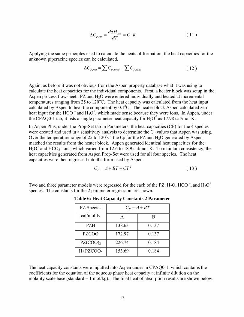
The heat capacity constants were inputted into Aspen under in CPAQ0-1, which contains the coefficients for the equation of the aqueous phase heat capacity at infinite dilution on the molality scale base (standard = 1 mol/kg). The final heat of absorption results are shown below.

18

Table 7: Reconciled Heat of Absorption Results

Temp oC

PCO2

Pa ∆H-HD

kcal/mol

∆H-VLE

kcal/mol

Diff

%

25 35.90 -20.16 -20.16 0.02

60 31183 -10.68 -10.62 -0.6

120 10637 -7.10 -6.88 -3.1

Preliminary results show that the overall absolute error is approximately ±6%. It was found that if the heat capacity for HCO3

- was manually adjusted, the absolute error could be reduced to about ±4%.

Conclusion and Future Work

It was found that by changing the charge of the H+PZCOO- species, the absolute trend for the heat of absorption was correctly obtained. The derivation of the heats of formation and heat capacities for the PZH+, PZCOO-, PZ(COO-)2, H+PZCOO- ions species from the equilibrium constant equations were used to make the K+/PZ VLE model internally consistent with the thermodynamics. The heats of absorption predicted by the CO2 vapor pressure data matched the heat duty generated by Aspen from flash calculation to within ±6%. The change in charge will require the re-regression of the VLE data in Aspen. Once this is done, the entire heat of absorption reconciliation process will be repeated.

Additional time may be spent with Aspen to decipher how the heat capacities for the H3O+ and HCO3

- are calculated and implemented in the Aspen Plus software. Absorber modeling using Aspen RateSep with activity-based kinetics will continue once the VLE data has been re-regressed with the updated charge correction.

References

Chen, C.-C., Email from Aspen Tech Regarding H+PZCOO- IONMOB Adjustments. In 2006.

Cullinane, J. T., Thermodynamics and Kinetics of Aqueous Piperazine with Potassium Carbonate for Carbon Dioxide Absorption. Ph.D. Dissertation, The University of Texas at Austin, Austin, 2005.

Hilliard, M., CO2 Capture by Absorption with Potassium Carbonate - First Quarterly Report; U.S. Dept. of Energy: 2003.

Hilliard, M., Thermodynamics of Aqueous Piperazine/Potassium Carbonate/Carbon Dioxide

Characterized by Electrolyte MRTL Model within Aspen Plus. M.S., The University of Texas at Austin, Austin, TX, 2005.

Smith, J. M., Van Ness, H. C., Abbott, M. M., Introduction to Chemical Engineering Thermodynamics. 5th ed.; McGraw-Hill Companies, Inc.: New York, 1996.

19

Subtask 1.3b – Rate-based Modeling – Aspen Custom Modeler for Stripper by Babatunde Oyenekan

(Supported by this contract)

Introduction

We have continued to develop the stripper submodel in Aspen Custom Modeler for the overall model of CO2 absorption/stripping for 7m monoethanolamine (MEA), 5m K+/2.5m PZ and some generic solvents. In this work, we present rate model results for the stripping of CO2 from a 5m K+/2.5m PZ solvent using IMTP #40 packing at 30 kPa and 160 kPa reboiler pressures. We have used the model to determine mass transfer mechanisms in the stripper and initiated optimization of the packing volume. A “short and fat” stripper was found to be preferable to a “tall and skinny” one. The vacuum stripper requires less equivalent work than the simple stripper when run at the same percent flood. The results show that the stripper is liquid film controlled. The stripper operation is kinetics controlled at 30 kPa and diffusion controlled at 160 kPa.

Experimental (Model Formulation)

Stripping can occur by three mechanisms in the stripper. These are flashing, which occurs at the stripper inlet and at the top section of the stripper leading to the generation of a lot of bubbles and mass transfer area, normal mass transfer on the surface of packings or on trays, and under boiling conditions in the reboiler. Modeling of stripping columns is essential so that the operation of the column could be understood, the energy requirement for stripping (which has been estimated to be ~ 80% of the operating cost of the absorption/stripping system) can be reduced, and so as to provide some understanding into the phenomenon of mass transfer with chemical reaction at stripper conditions. Three main approaches are used in stripper modeling – equilibrium-stage modeling, mass transfer with equilibrium reactions, and mass transfer with reaction in the boundary layer and liquid diffusion.

Equilibrium Modeling

In this approach, infinite mass transfer is assumed. The stripping column is divided into a user-defined number of sections assumed to be well mixed in the liquid and vapor phases. The reboiler is assumed to be an equilibrium stage. Murphree efficiencies are assigned to components and temperature to account for the departure from equilibrium. This approach is useful in carrying out quick evaluations of process concepts but does not describe a real process. Only the conventional MESH (material, equilibrium, summation, and enthalpy) equations are solved using this approach. This approach has been used in our previous work1, 2.

Rate (non-equilibrium) Modeling

This approach takes into account that the rate of desorption is finite and that the transfer of CO2 is governed by mass transfer rate and not equilibrium considerations. In addition to the conventional MESH equations, the mass and heat transfer rate equations are solved. Rate-based modeling allows for insight into the fundamental mechanisms of mass transfer and could help predict the operation of a constant diameter column as well as aid in the design of columns with variable diameter at constant percent flood.

20

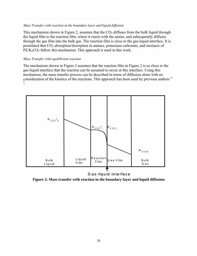
Mass Transfer with reaction in the boundary layer and liquid diffusion

This mechanism shown in Figure 2, assumes that the CO2 diffuses from the bulk liquid through the liquid film to the reaction film, where it reacts with the amine, and subsequently diffuses through the gas film into the bulk gas. The reaction film is close to the gas-liquid interface. It is postulated that CO2 absorption/desorption in amines, potassium carbonate, and mixtures of PZ/K2CO3 follow this mechanism. This approach is used in this work. Mass Transfer with equilibrium reaction

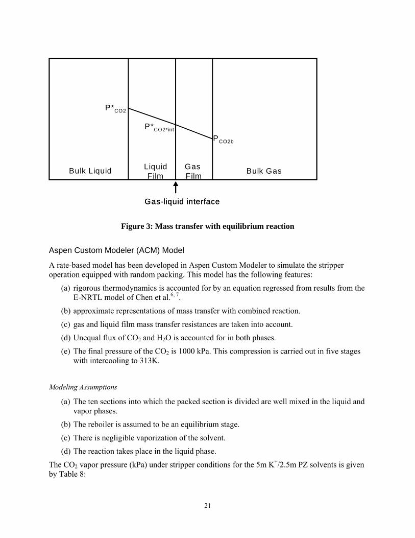
The mechanism shown in Figure 3 assumes that the reaction film in Figure 2 is so close to the gas-liquid interface that the reaction can be assumed to occur at this interface. Using this mechanism, the mass transfer process can be described in terms of diffusion alone with no consideration of the kinetics of the reactions. This approach has been used by previous authors 3-

5.

Figure 2: Mass transfer with reaction in the boundary layer and liquid diffusion

B u lk G a s

G a s F ilmR e a c t io n

F ilmL iq u id F ilm

B u lkL iq u id

P C O 2 b

P C O 2 ,iP C O 2 * i

P C O 2 * b

G a s - l iq u id in te r fa c e

B u lk G a s

G a s F ilmR e a c t io n

F ilmL iq u id F ilm

B u lkL iq u id

P C O 2 b

P C O 2 ,iP C O 2 * i

P C O 2 * b

B u lk G a s

G a s F ilmR e a c t io n

F ilmL iq u id F ilm

B u lkL iq u id

P C O 2 b

P C O 2 ,iP C O 2 * i

P C O 2 * b

B u lk G a s

G a s F ilmR e a c t io n

F ilmL iq u id F ilm

B u lkL iq u id

P C O 2 b

P C O 2 ,iP C O 2 * i

P C O 2 * b

G a s - l iq u id in te r fa c e

21

Figure 3: Mass transfer with equilibrium reaction

Aspen Custom Modeler (ACM) Model

A rate-based model has been developed in Aspen Custom Modeler to simulate the stripper operation equipped with random packing. This model has the following features:

(a) rigorous thermodynamics is accounted for by an equation regressed from results from the E-NRTL model of Chen et al.6, 7.

(b) approximate representations of mass transfer with combined reaction.

(c) gas and liquid film mass transfer resistances are taken into account.

(d) Unequal flux of CO2 and H2O is accounted for in both phases.

(e) The final pressure of the CO2 is 1000 kPa. This compression is carried out in five stages with intercooling to 313K.

Modeling Assumptions

(a) The ten sections into which the packed section is divided are well mixed in the liquid and vapor phases.

(b) The reboiler is assumed to be an equilibrium stage.

(c) There is negligible vaporization of the solvent.

(d) The reaction takes place in the liquid phase.

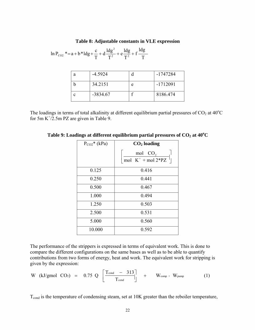
The CO2 vapor pressure (kPa) under stripper conditions for the 5m K+/2.5m PZ solvents is given by Table 8:

Bulk GasGasFilm

Liquid Film

PCO2b

P*CO2,int

Bulk Liquid

Gas-liquid interface

P*CO2

Bulk GasGasFilm

Liquid Film

PCO2b

P*CO2,int

Bulk Liquid

Gas-liquid interface

P*CO2

22

Table 8: Adjustable constants in VLE expression

T

ldgf

Tldge

Tldgd

Tcldg*ba*Pln 22

2

CO2 +++++=

a -4.5924 d -1747284

b 34.2151 e -1712091

c -3834.67 f 8186.474

The loadings in terms of total alkalinity at different equilibrium partial pressures of CO2 at 40oC for 5m K+/2.5m PZ are given in Table 9.

Table 9: Loadings at different equilibrium partial pressures of CO2 at 40oC

PCO2* (kPa) CO2 loading

2+

mol COmol K + mol 2*PZ

⎡ ⎤⎢ ⎥⎣ ⎦

0.125 0.416

0.250 0.441

0.500 0.467

1.000 0.494

1.250 0.503

2.500 0.531

5.000 0.560

10.000 0.592

The performance of the strippers is expressed in terms of equivalent work. This is done to compare the different configurations on the same bases as well as to be able to quantify contributions from two forms of energy, heat and work. The equivalent work for stripping is given by the expression:

cond2 comp + pump

cond

T 313W (kJ/gmol CO ) 0.75 Q W WT

−⎡ ⎤= +⎢ ⎥⎣ ⎦ (1)

Tcond is the temperature of condensing steam, set at 10K greater than the reboiler temperature,

23

Wcomp is the work of compression with a 75% efficiency and Wpump is the work required by the pumps with a 65% efficiency.

The flux of CO2 is given by the expression:

NCO2 = KG (PCO2* - PCO2) (2)

The overall mass transfer coefficient (KG) is the sum of the gas phase (kg) and liquid phase (kg’) components.

'k

1k1

K1

ggG

+= (3)

The hydraulic parameters kga, kla are obtained from Onda8 while the area, a, was obtained from tests at the University of Texas Separations Research Program. The liquid phase mass transfer coefficient defined in terms of partial pressure driving forces, kg’, is calculated by an equation regressed from Cullinane9 and is a function of the loading, temperature, and partial pressure of CO2 at the interface.The CO2 desorption rate is:

Rate = KG A (PCO2* - PCO2) (4)

The wetted area of contact, A, depends on the equipment and hydraulics in the column. The overall mass transfer coefficient, KG, for mass transfer with reaction in the boundary layer and liquid diffusion is given by:

*

T2

CO2

prodl,CO2i2

CO2

gG ]∆[CO∆P

k1

D[Am]kH

k1

K1

⎟⎟⎠

⎞⎜⎜⎝

⎛++= (5)

with HCO2 being the Henry’s law constant for CO2,k2, the reaction rate constant, [Am]I, the concentration of amine at the interface, DCO2, the diffusivity of CO2, kl, prod, the liquid mass transfer coefficient of the products which is assumed to be equal for all products, [CO2]T, the total concentration of CO2 in all forms. The term in the bracket in the third term on the right hand side of equation 5 is the secant of the equilibrium curve. If the reaction occurs very fast so that the rate constant, k2, is very large, then the second term on the right hand side of equation (4) drops out and we have the expression for KG for mass transfer with equilibrium reaction given by:

*

T2

CO2

prodl,gG ]∆[CO∆P

k1

k1

K1

⎟⎟⎠

⎞⎜⎜⎝

⎛+= (6)

The model inputs were the rich and lean loadings, the liquid rate, the temperature approach in the cross exchanger (difference between the temperature of the rich stripper feed and the lean solution leaving the bottom of the stripper), and column pressure. Initial guesses of the segment temperatures, partial pressures, and loadings were provided. The model solves the MESH

24

equations, the mass and energy transfer rate equations, and calculates temperature and composition profiles, reboiler duty, and equivalent work.

Results and Discussion

Predicted Stripper Performance from Rate-Based Model

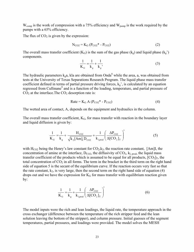
For a rate-based (non-equilibrium) model, the percent flood was specified. For a specified rich and lean loading, 0.560 (rich) and 0.467 (lean) mol CO2/mol Total Alkalinity, the diameter and height of the column required to achieve the separation with a fixed volume of packing was calculated. The results are shown in Table 10. At a fixed percent flood, a “short and fat” column is required to perform the separation in the vacuum stripper relative to the simple stripper. The reboiler duty is higher with the vacuum stripper but since the steam required to drive the reboiler has a less work value under vacuum conditions (30 kPa) than at 160 kPa, the total equivalent work is less with the vacuum stripper even though the work of compression is more. At a fixed percent flood, the vacuum stripper operation requires ~ 7% less equivalent work than the simple one.

Table 10: “Short and Fat” vs. “Tall and Skinny” Column

(5m K+/2.5m PZ, L=30 gpm, Rich ldg = 0.560, Lean ldg = 0.467 mol CO2/mol Total Alk, Tapp = 5oC, Fixed Volume of Packing = 0.858 m3)

Reboiler P % flood D H Qreb Wcomp Total Weq

kPa m kJ/mol

80 0.33 9.8 190 18 33.7 30

30 0.51 4.2 155 15 30.9

80 0.20 26.8 138 7.6 35.3 160

30 0.33 10.2 128 7 33.3

McCabe-Thiele plots give an indication of the internal operation of the column and could help understand column behavior. The McCabe-Thiele plot for the vacuum stripper is shown in Figure 4. The rich solution flashes at the top of the stripper and the temperature drops at the rich end. The top half of the column is pinched. The bottom half exhibits a well defined driving force. The bulk of the stripping operation takes place in the reboiler. This could be a consequence of the reboiler being treated as an equilibrium stage in the model. The McCabe-Thiele plot for the simple stripper is shown in Figure 5. The rich solution flashes to a much greater degree than in the vacuum case. This is because the pressure and temperature are higher and as such the partial pressure of the rich solution is significantly higher in the simple stripper than in the vacuum case. The stripping operation occurs mainly as a result of flashing and in the reboiler. This may constitute a sub-optimal case as this implies that the amount of packing used in this stripper is a lot more than required and as such there are sections of packing in which little or no stripping occurs.

25

Figure 4: McCabe-Thiele plot for vacuum stripper (Rich ldg= 0.560, lean ldg= 0.467, Tapp= 5oC)

The mass transfer mechanisms in the stripper were also investigated. The liquid phase mass transfer coefficient, ky’, and the overall mass transfer coefficient, Ky’, based on mole fraction units for the vacuum and simple strippers are shown in Table 11. The results show that the rates increase from the rich to the lean end by over a factor of 2 for the vacuum case and about 1.5 for the simple case. The rate increases because as we go down the column from the rich end to the lean end, there is more free amine available for reaction. The rates in the simple stripper are also an order of magnitude greater than the vacuum case. This is as a result of the high temperatures that increase the reaction rate constant at high pressures. The table also shows that kinetic resistance has the largest contribution (89% at the rich end and 60% at the lean end) to the overall mass transfer rate under vacuum conditions while the diffusion of products is more important in the simple stripper accounting for 69% at the rich end and 50% at the lean end.

Conclusions and Future Work

In this quarter, a rate model was developed in Aspen Custom Modeler (ACM). This model was used to determine favorable design orientations for the stripper and to understand mass transfer mechanisms for stripping operations using 5m K+/2.5m PZ as the solvent. The results show that a “short and fat” stripper is more attractive than a “tall and skinny one.” The pressure drop is also less with a “short and fat” stripper. At a fixed percent flood, the vacuum stripper requires ~ 7% less equivalent work than the simple one. The stripper operation was found to be liquid film controlled. The vacuum stripper was kinetic controlled while the simple stripper was diffusion controlled.

In the next quarter, the packing volume will be optimized and the pilot plant campaign results will be revisited in order to interpret the results, which will help in the fine-tuning of the model.

0

10

20

30

40

50

60

30

40

50

60

70

0.46 0.48 0.5 0.52 0.54 0.56 0.58

PC

O2 (k

Pa) T ( oC

)

ldg (mol CO2/mol TAlk)

T

Operating Line

PCO2

Equilibrium LineP

CO2*

26

Figure 5: McCabe-Thiele plot for simple stripper (Rich ldg = 0.560, lean ldg = 0.467, Tapp = 5oC)

Table 11: Mass transfer mechanisms in strippers

Mole fraction units (x105) kmol/m2-s

P = 30 kPa P = 160 kPa

Rich End Lean End Rich End Lean End

ky’ 1.5 3.7 22.8 37.7

Ky’ 1.5 3.5 19.8 28.0

Gas Res. (%) 2 3 14 25

Kinetic Res. (%) 89 60 17 25

Diffusion Res. (%) 9 37 69 50

Subtask 1.8a – Alternative stripper configurations – Aspen Custom Modeler for Stripper by Babatunde Oyenekan

(Supported by this contract)

Introduction We have continued to develop the stripper submodel in Aspen Custom Modeler for the overall model of CO2 absorption/stripping for 7m monoethanolamine (MEA), 5m K+/2.5m PZ and some generic solvents. In this quarter, four new stripper configurations (matrix, internal exchange,

0

100

200

300

400

500

600

700

60

80

100

120

0.46 0.48 0.5 0.52 0.54 0.56 0.58

PC

O2 (k

Pa) T ( oC

)

ldg (mol CO2 / mol TAlk)

Operating Line

PCO2

Equilibrium Line

PCO2

*

T

27

flashing feed, and multipressure with split feed) have been evaluated with five different solvents: 7m (30 wt%) monoethanolamine (MEA), potassium carbonate promoted by piperazine (PZ), promoted MEA, methyldiethanolamine (MDEA) promoted by PZ, and hindered amines. The results show solvents with low heats of absorption (PZ/K2CO3) favor vacuum operation while solvents with high heats of absorption (MEA, MEA/PZ) favor operation at normal pressure. The relative performance of the alternative configurations is matrix > internal exchange > multipressure with split feed > flashing feed. MEA/PZ and MDEA/PZ are attractive alternatives to 7m MEA. The best solvent and process configuration, matrix with MDEA/PZ, offers 22% and 15% energy savings over the baseline and improved baseline respectively with stripping and compression to 10 MPa. The energy requirement for stripping and compression to 10 MPa is about 20% of the power output from a 500 MW power plant with 90% CO2 removal.

Experimental (Model Formulation) Solvent Alternatives The solvents investigated are seven potential solvent compositions better viewed as generic solvents giving specific heats of absorption (∆Habs), capacity and rates of reaction with CO2. The vapor-liquid equilibrium (VLE) representation of the solvents was obtained from different sources. The heat of desorption was obtained by differentiating the VLE expression with respect to the inverse of temperature. The capacity of the solution is given by:

OHkgAlkmol

AlkmolCOmol

γOHkg

COmolcapacity

2

2

2

2⎟⎟⎠

⎞⎜⎜⎝

⎛=⎟⎟

⎠

⎞⎜⎜⎝

⎛ (1)

Moles of Alkalinity (mol Alk) is given by:

Mol Alk = mol MEA + mol K+ + mol 2 PZ + mol MDEA + mol KS-1 (2)

The solvent alternatives are three promoted K2CO3 formulations (6.4m K+/1.6m PZ, 5m K+/2.5m PZ,4.5m K+/4.5m PZ), promoted MEA (MEA/PZ), promoted tertiary amine (MDEA/PZ), and hindered amine (KS-1). The vapor/liquid equilibrium representation of these solvents was obtained from a variety of sources1. The alternative configurations and model development are detailed in Oyenekan and Rochelle (2006)1.

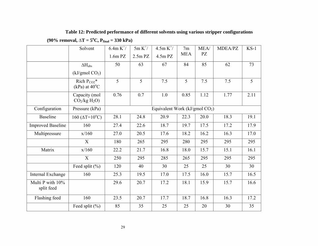
Results and Discussion Predicted Stripper Performance for Different Configurations Table 12 shows the performance of seven potential solvents. The solvent properties are approximate and not necessarily accurate representations of the specific solvents but can be viewed as surrogates. The table can be used to study the influence of a wide range of heats of absorption (∆Habs) from 50-85 kJ/gmol CO2. Two levels of rates of reaction of the solvents with CO2, quantified in terms of rich PCO2* @ 40oC, are shown in the table. The rich PCO2* = 5 kPa solvents represent solvents with approximately equivalent rates while those with rich PCO2* = 7.5 kPa represent faster solvents. The capacities in the table are those that correspond to a 90% reduction in the rich PCO2*. A wide range of capacities (0.7 – 2.11 mol CO2/kg H2O) was studied.

28

Solvent Performance

MEA/PZ and MDEA/PZ require significantly less equivalent work than 7m MEA at 160 kPa. MEA/PZ offers a 13% and 8% savings over 7m MEA with the matrix and internal exchange configurations at 160 kPa. MDEA/PZ was the most attractive solvent under vacuum conditions. MDEA/PZ offers a 14% and 10% savings over 7m MEA with the matrix and internal exchange configurations at 30 kPa. This shows that, at normal pressure, solvents with high heats of absorption and reasonable capacities are attractive. Under vacuum conditions, solvents with lower heats of absorption and higher capacities are attractive. Capacity seems to play a more important role in determining energy requirements at vacuum conditions. Effect of heat of absorption

Comparing 6.4m K+/1.6m PZ and 5m K+/2.5m PZ, solvents with similar capacities but different heats of absorption are compared. The results show that at a fixed capacity, solvents with high heats of absorption require less energy for stripping. This is a consequence of the temperature swing. The 5m K+/2.5m PZ offers 18% savings over 6.4m K+/1.6m PZ at 160 kPa with a 5oC approach. Effect of capacity

5m K+/2.5m PZ and MDEA/PZ have similar heats of absorption, however MDEA/PZ has a greater capacity than 5m K+/2.5m PZ. MDEA/PZ provides 30% and 19% energy savings over 5m K+/2.5m PZ with the matrix and internal exchange configurations with the reboiler operating at 160 kPa and 17% and 12% savings with these configurations at 30 kPa. The two MEA solvents also have similar heats of absorption. MEA/PZ represented by 11.4 m MEA has a higher capacity than 7m MEA. MEA/PZ offers 13% energy savings over 7m MEA with the matrix stripper operated with a 160 kPa reboiler temperature. Effect on power plant output and process improvement

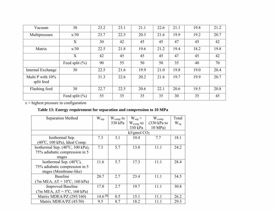
Different separation techniques are compared by separation and compression work in Table 13. The total equivalent work for isothermal separation at 100 kPa and 40oC and subsequent compression to 10 MPa is 18.1 kJ/gmol CO2. This is the theoretical minimum work for separation and compression to 10 MPa, and constitutes about 12% of the power plant output. If five compressors with 75% adiabatic efficiency are used, the total equivalent work is 24.2 kJ/gmol CO2 (16% of the power plant output). If isothermal separation at 40oC with 75% adiabatic compression in five stages is used, the total equivalent work is 28.4 kJ/gmol CO2. This can be likened to separation with a perfect membrane.

The best solvent and process configuration is the matrix (295/160 kPa) with MDEA/PZ. This consumes 26.2 kJ/gmol CO2 (18% of the net output from a 500 MW power plant with 90% CO2 capture). This best case offers 22% energy savings over the current industrial baseline (7m MEA, ∆T = 10oC, 160 kPa) and 15% savings over the improved baseline (7m MEA, ∆T = 5oC, 160 kPa). It requires 2 kJ/gmol CO2 more work than the theoretical minimum with real compressors. Therefore, there is little room for improvement

Based on process analysis and economic studies2, the net power output of a 500 MW power plant is about 150 kJ/gmol CO2 with 90% CO2 removal. The typical energy requirement for stripping and compression is about 30 kJ/gmol CO2.

29

Table 12: Predicted performance of different solvents using various stripper configurations

(90% removal, ∆T = 5oC, Pfinal = 330 kPa)

Solvent 6.4m K+/

1.6m PZ

5m K+/

2.5m PZ

4.5m K+/

4.5m PZ

7m MEA

MEA/PZ

MDEA/PZ KS-1

∆Habs

(kJ/gmol CO2)

50 63 67 84 85 62 73

Rich PCO2* (kPa) at 40oC

5 5 7.5 5 7.5 7.5 5

Capacity (mol CO2/kg H2O)

0.76 0.7 1.0 0.85 1.12 1.77 2.11

Configuration Pressure (kPa) Equivalent Work (kJ/gmol CO2)

Baseline 160 (∆T=10oC) 28.1 24.8 20.9 22.3 20.0 18.3 19.1

Improved Baseline 160 27.4 22.6 18.7 19.7 17.5 17.2 17.9

Multipressure x/160 27.0 20.5 17.6 18.2 16.2 16.3 17.0

X 180 265 295 280 295 295 295

Matrix x/160 22.2 21.7 16.8 18.0 15.7 15.1 16.1

X 250 295 285 265 295 295 295

Feed split (%) 120 40 30 25 25 30 30

Internal Exchange 160 25.3 19.5 17.0 17.5 16.0 15.7 16.5

Multi P with 10% split feed

29.6 20.7 17.2 18.1 15.9 15.7 16.6

Flashing feed 160 23.5 20.7 17.7 18.7 16.8 16.3 17.2

Feed split (%) 85 35 25 25 20 30 35

30

Vacuum 30 23.2 23.1 21.1 22.6 21.1 19.8 21.2

Multipressure x/30 23.7 22.5 20.3 21.6 19.9 19.2 20.7

X 30 42 45 45 47 45 42

Matrix x/30 22.5 21.8 19.6 21.2 19.4 18.2 19.8

X 42 45 45 45 47 45 42

Feed split (%) 90 55 50 50 35 40 70

Internal Exchange 30 22.5 21.6 19.9 21.0 19.8 19.0 20.4

Multi P with 10% split feed

31.3 22.6 20.2 21.6 19.7 19.9 20.7

Flashing feed 30 22.7 22.5 20.6 22.1 20.6 19.5 20.8

Feed split (%) 55 35 35 35 30 35 45

x = highest pressure in configuration

Table 13: Energy requirement for separation and compression to 10 MPa

Separation Method Wsep Wcomp to 330 kPa

Wsep + Wcomp to 330 kPa

Wcomp (330 kPa to

10 MPa)

Total Weq

kJ/gmol CO2 Isothermal Sep.

(40oC, 100 kPa), Ideal Comp. 7.3 3.1 10.4 7.7 18.1

Isothermal Sep. (40oC, 100 kPa), 75% adiabatic compression in 5

stages

7.3 5.7 13.0 11.1 24.2

Isothermal Sep. (40oC), 75% adiabatic compression in 5

stages (Membrane-like)

11.6 5.7 17.3 11.1 28.4

Baseline (7m MEA, ∆T = 10oC, 160 kPa)

20.7 2.7 23.4 11.1 34.5

Improved Baseline (7m MEA, ∆T = 5oC, 160 kPa)

17.0 2.7 19.7 11.1 30.8

Matrix MDEA/PZ (295/160) 14.6 0.5 15.1 11.1 26.2 Matrix MDEA/PZ (45/30) 9.5 8.7 18.2 11.1 29.3

31

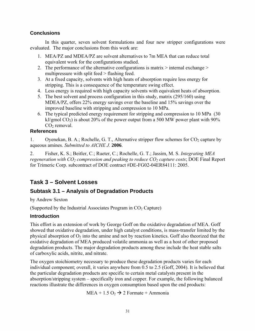
Conclusions

In this quarter, seven solvent formulations and four new stripper configurations were evaluated. The major conclusions from this work are:

1. MEA/PZ and MDEA/PZ are solvent alternatives to 7m MEA that can reduce total equivalent work for the configurations studied.

2. The performance of the alternative configurations is matrix > internal exchange > multipressure with split feed > flashing feed.

3. At a fixed capacity, solvents with high heats of absorption require less energy for stripping. This is a consequence of the temperature swing effect.

4. Less energy is required with high capacity solvents with equivalent heats of absorption. 5. The best solvent and process configuration in this study, matrix (295/160) using

MDEA/PZ, offers 22% energy savings over the baseline and 15% savings over the improved baseline with stripping and compression to 10 MPa.

6. The typical predicted energy requirement for stripping and compression to 10 MPa (30 kJ/gmol CO2) is about 20% of the power output from a 500 MW power plant with 90% CO2 removal.

References 1. Oyenekan, B. A.; Rochelle, G. T., Alternative stripper flow schemes for CO2 capture by aqueous amines. Submitted to AICHE J. 2006.

2. Fisher, K. S.; Beitler, C.; Rueter, C.; Rochelle, G. T.; Jassim, M. S. Integrating MEA regeneration with CO2 compression and peaking to reduce CO2 capture costs; DOE Final Report for Trimeric Corp. subcontract of DOE contract #DE-FG02-04ER84111: 2005.

Task 3 – Solvent Losses Subtask 3.1 – Analysis of Degradation Products by Andrew Sexton

(Supported by the Industrial Associates Program in CO2 Capture)

Introduction This effort is an extension of work by George Goff on the oxidative degradation of MEA. Goff showed that oxidative degradation, under high catalyst conditions, is mass-transfer limited by the physical absorption of O2 into the amine and not by reaction kinetics. Goff also theorized that the oxidative degradation of MEA produced volatile ammonia as well as a host of other proposed degradation products. The major degradation products among these include the heat stable salts of carboxylic acids, nitrite, and nitrate.

The oxygen stoichiometry necessary to produce these degradation products varies for each individual component; overall, it varies anywhere from 0.5 to 2.5 (Goff, 2004). It is believed that the particular degradation products are specific to certain metal catalysts present in the absorption/stripping system – specifically iron and copper. For example, the following balanced reactions illustrate the differences in oxygen consumption based upon the end products:

MEA + 1.5 O2 2 Formate + Ammonia

32

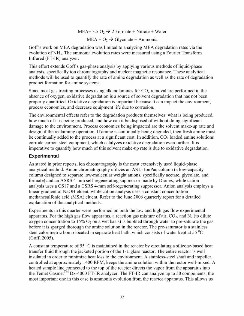
MEA+ 3.5 O2 2 Formate + Nitrate + Water

MEA + O2 Glycolate + Ammonia

Goff’s work on MEA degradation was limited to analyzing MEA degradation rates via the evolution of NH3. The ammonia evolution rates were measured using a Fourier Transform Infrared (FT-IR) analyzer.

This effort extends Goff’s gas-phase analysis by applying various methods of liquid-phase analysis, specifically ion chromatography and nuclear magnetic resonance. These analytical methods will be used to quantify the rate of amine degradation as well as the rate of degradation product formation for amine systems.

Since most gas treating processes using alkanolamines for CO2 removal are performed in the absence of oxygen, oxidative degradation is a source of solvent degradation that has not been properly quantified. Oxidative degradation is important because it can impact the environment, process economics, and decrease equipment life due to corrosion.

The environmental effects refer to the degradation products themselves: what is being produced, how much of it is being produced, and how can it be disposed of without doing significant damage to the environment. Process economics being impacted are the solvent make-up rate and design of the reclaiming operation. If amine is continually being degraded, then fresh amine must be continually added to the process at a significant cost. In addition, CO2 loaded amine solutions corrode carbon steel equipment, which catalyzes oxidative degradation even further. It is imperative to quantify how much of this solvent make-up rate is due to oxidative degradation.

Experimental As stated in prior reports, ion chromatography is the most extensively used liquid-phase analytical method. Anion chromatography utilizes an AS15 IonPac column (a low-capacity column designed to separate low-molecular weight anions, specifically acetate, glycolate, and formate) and an ASRS 4-mm self-regenerating suppressor made by Dionex, while cation analysis uses a CS17 and a CSRS 4-mm self-regenerating suppressor. Anion analysis employs a linear gradient of NaOH eluent, while cation analysis uses a constant concentration methanesulfonic acid (MSA) eluent. Refer to the June 2006 quarterly report for a detailed explanation of the analytical methods.

Experiments in this quarter were performed on both the low and high gas flow experimental apparatus. For the high gas flow apparatus, a reaction gas mixture of air, CO2, and N2 (to dilute oxygen concentration to 15% O2 on a wet basis) is bubbled through water to pre-saturate the gas before it is sparged thorough the amine solution in the reactor. The pre-saturator is a stainless steel calorimetric bomb located in separate heat bath, which consists of water kept at 55 oC (Goff, 2005).

A constant temperature of 55 oC is maintained in the reactor by circulating a silicone-based heat transfer fluid through the jacketed portion of the 1-L glass reactor. The entire reactor is well insulated in order to minimize heat loss to the environment. A stainless-steel shaft and impeller, controlled at approximately 1400 RPM, keeps the amine solution within the rector well-mixed. A heated sample line connected to the top of the reactor directs the vapor from the apparatus into the Temet GasmetTM Dx-4000 FT-IR analyzer. The FT-IR can analyze up to 50 components; the most important one in this case is ammonia evolution from the reactor apparatus. This allows us

33

to assume an amine degradation rate. Refer to Chapter 3 of Goff (2005) for a more in-depth explanation of how this apparatus operates.

As stated in previous reports, amine solutions in the low gas flow degradation apparatus are oxidized for 12 to 14 days in a low gas flow jacketed reactor at 55oC. The solutions are agitated at 1400 RPM to produce a high level of gas/liquid mass transfer by vortexing. 98% O2/2% CO2 at 100 ml/min is introduced across the vortexed surface of 350 ml of aqueous amine. Samples were taken from the reactor at regular intervals in order to determine how degradation products formed over the course of the experiment. Prior quarterly reports provide a detailed explanation of the low gas flow degradation apparatus.

Results Using the analytical methods for the AS15 and CS17 columns, the following degradation experiments are being analyzed for degradation product formation rates:

1. September 2006 MEA experiment (Oxidative degradation of 35 wt % MEA, 55oC, 1400 RPM, 5 ppm Fe, 0.4 moles CO2/mol MEA, 98%O2/2%CO2).

2. September 2006 MEA/PZ experiment (Oxidative degradation of 7 m MEA / 2 m PZ, 55oC, 1400 RPM, 5 ppm Fe, 250 ppm Cu, 98%O2/2%CO2).

Analysis was performed on these experiments, which were conducted during the prior quarters:

1. April 2006 MEA/PZ experiment (Oxidative degradation of 7 m MEA/2 m PZ, 55oC, 1400 RPM, 98%O2/2%CO2).

2. March/April 2006 PZ experiment (Oxidative degradation of 2.5 m piperazine/5 m KHCO3, 55oC, 1400 RPM, 500 ppm V+, 98%O2/2%CO2).

3. November 2005 PZ experiment (Oxidative degradation of 2.5 m piperazine, 55oC, 1400 RPM, 500 ppm V+, 98%O2/2%CO2).

In addition, several experiments were run using the high gas flow degradation apparatus – some at proprietary conditions, and other at conditions that are within this report. Three reportable experiments involved 7 m MEA; in addition, two MEA/PZ blends were subjected to oxidative degradation. Three MEA experiments were run at the following conditions:

1. 0.1 mM Fe – This simulates a commercial system in which Fe is being continuously removed from the system to keep iron concentration at minimal levels.

2. 1 mM Fe – This simulates an iron concentration in normal commercial systems.

3. 0.1 mM Fe, 5 mM Fe – This simulates catalyst conditions found in commercial systems where copper is added to reduce iron concentration, thereby inhibiting corrosion.

The MEA/PZ blends were run at the following conditions:

1. 4.6 m MEA/1.2 m PZ (22 wt % MEA/8 wt % PZ), 0.1 mM Fe – This simulates a commercial system in which Fe is being continuously removed from the system to minimize corrosion rates.

2. 7 m MEA/2 m PZ (27 wt % MEA/11 wt % PZ), 0.1 mM Fe, 5 mM Cu – This simulates a commercial system in which copper is added as a corrosion inhibitor.

34

All solutions were run for 12 to 14 hours in the high gas flow apparatus and the off-gas was continuously analyzed by the FT-IR. Liquid-phase samples were taken at the beginning and end of each experiment and subjected to IC analysis.

Table 14 lists oxidative degradation product formate rates for the three aforementioned low gas flow degradation experiments. All rates for the PZ/V+ experiment have been posted previously, with the exception of the ammonium rate – which has been discovered this quarter as a product of piperazine degradation (0.031 mM/hr). Ammonium analysis for the other two experiments is not available because the current method cannot analyze for ammonium under the presence of large quantities of potassium or MEA. The large MEA/potassium peak overlaps the small ammonium peak so that it cannot be detected.

For the K+/PZ solutions and MEA/PZ solutions, degradation rates are relatively low. This can be explained by the fact that the high K+ concentration reduces oxygen solubility in solution. The most abundant degradation product is nitrate (0.19 mM/hr). The other detectable degradation products are at rates less than 0.05 mM/hr. In the case of the MEA/PZ solution, all degradation product formation rates are below 0.04 mM/hr. The most concentrated product is formate at 0.034 mM/hr. The presence of EDA (at a production rate of 0.008 mM/hr) suggests that the piperazine is degrading, albeit at a very slow rate.

Table 14: Low Gas Flow Degradation Product Rates

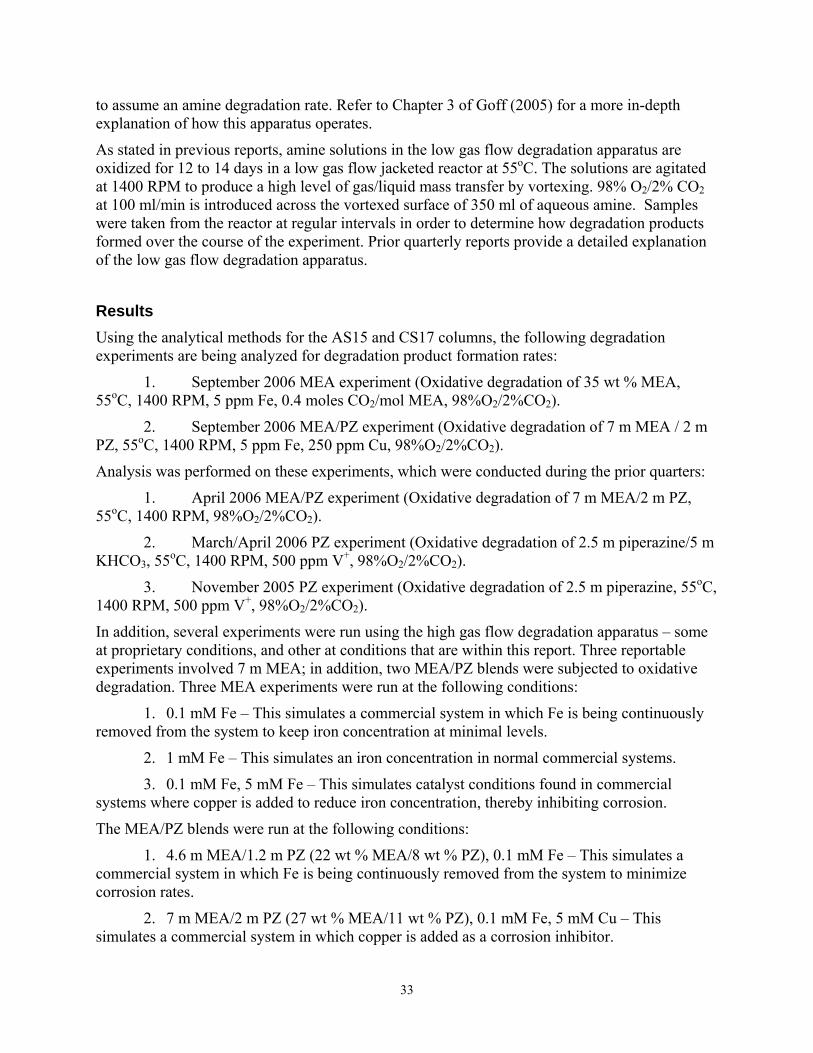
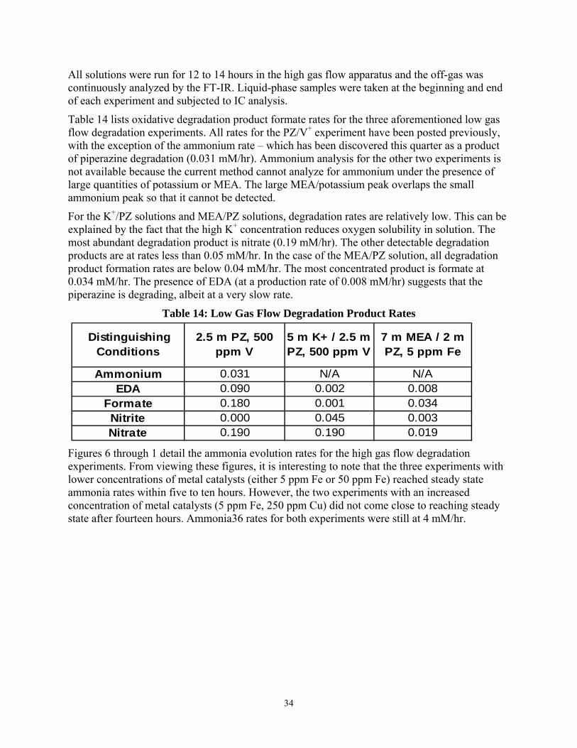
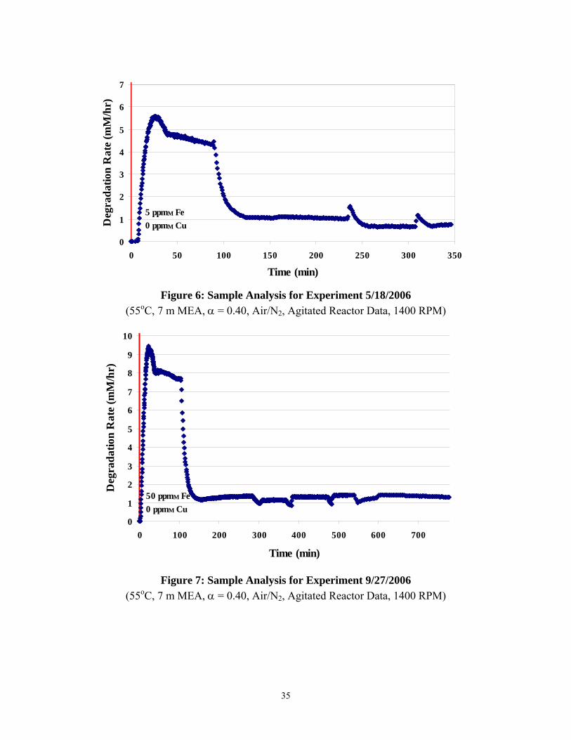
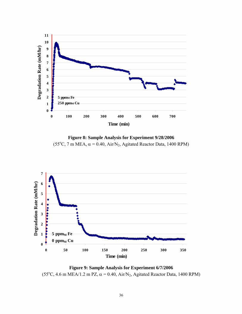
Figures 6 through 1 detail the ammonia evolution rates for the high gas flow degradation experiments. From viewing these figures, it is interesting to note that the three experiments with lower concentrations of metal catalysts (either 5 ppm Fe or 50 ppm Fe) reached steady state ammonia rates within five to ten hours. However, the two experiments with an increased concentration of metal catalysts (5 ppm Fe, 250 ppm Cu) did not come close to reaching steady state after fourteen hours. Ammonia36 rates for both experiments were still at 4 mM/hr.

Distinguishing

Conditions2.5 m PZ, 500

ppm V5 m K+ / 2.5 m PZ, 500 ppm V

7 m MEA / 2 m PZ, 5 ppm Fe

Ammonium 0.031 N/A N/AEDA 0.090 0.002 0.008

Formate 0.180 0.001 0.034Nitrite 0.000 0.045 0.003Nitrate 0.190 0.190 0.019

35

0

1

2

3

4

5

6

7

0 50 100 150 200 250 300 350

Time (min)

Deg

rada

tion

Rat

e (m

M/h

r)

5 ppmM Fe0 ppmM Cu

Figure 6: Sample Analysis for Experiment 5/18/2006

(55oC, 7 m MEA, α = 0.40, Air/N2, Agitated Reactor Data, 1400 RPM)

0

1

2

3

4

5

6

7

8

9

10

0 100 200 300 400 500 600 700

Time (min)

Deg

rada

tion

Rat

e (m

M/h

r)

50 ppmM Fe0 ppmM Cu

Figure 7: Sample Analysis for Experiment 9/27/2006

(55oC, 7 m MEA, α = 0.40, Air/N2, Agitated Reactor Data, 1400 RPM)

36

0

1

2

3

4

5

6

7

8

9

10

11

0 100 200 300 400 500 600 700

Time (min)

Deg

rada

tion

Rat

e (m

M/h

r)

5 ppmM Fe250 ppmM Cu

Figure 8: Sample Analysis for Experiment 9/28/2006

(55oC, 7 m MEA, α = 0.40, Air/N2, Agitated Reactor Data, 1400 RPM)

0

1

2

3

4

5

6

7

0 50 100 150 200 250 300 350

Time (min)

Deg

rada

tion

Rat

e (m

M/h

r)

5 ppmM Fe0 ppmM Cu

Figure 9: Sample Analysis for Experiment 6/7/2006

(55oC, 4.6 m MEA/1.2 m PZ, α = 0.40, Air/N2, Agitated Reactor Data, 1400 RPM)

37

0

2

4

6

8

10

12

14

0 100 200 300 400 500 600 700

Time (min)

Deg

rada

tion

Rat

e (m

M/h

r)

5 ppmM Fe250 ppmM Cu

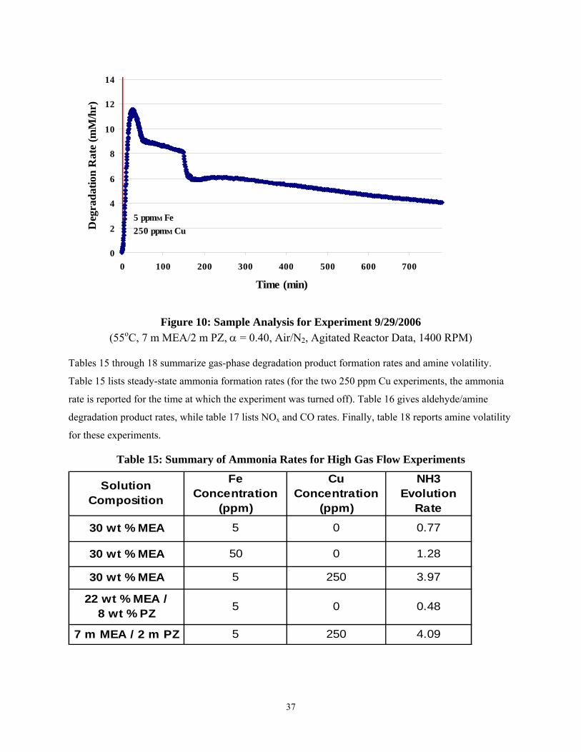
Figure 10: Sample Analysis for Experiment 9/29/2006

(55oC, 7 m MEA/2 m PZ, α = 0.40, Air/N2, Agitated Reactor Data, 1400 RPM)

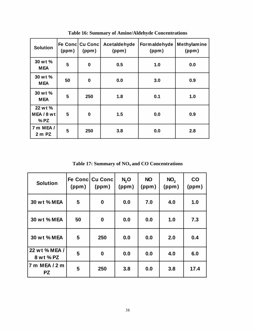
Tables 15 through 18 summarize gas-phase degradation product formation rates and amine volatility.

Table 15 lists steady-state ammonia formation rates (for the two 250 ppm Cu experiments, the ammonia

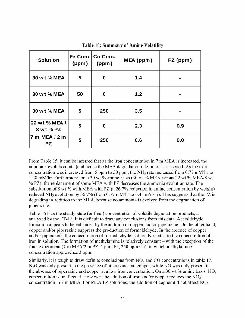
rate is reported for the time at which the experiment was turned off). Table 16 gives aldehyde/amine

degradation product rates, while table 17 lists NOx and CO rates. Finally, table 18 reports amine volatility

for these experiments.

Table 15: Summary of Ammonia Rates for High Gas Flow Experiments

Solution

Composition

Fe Concentration

(ppm)

Cu Concentration

(ppm)

NH3 Evolution

Rate

30 wt % MEA 5 0 0.77

30 wt % MEA 50 0 1.28

30 wt % MEA 5 250 3.97

22 wt % MEA / 8 wt % PZ 5 0 0.48

7 m MEA / 2 m PZ 5 250 4.09

38

Table 16: Summary of Amine/Aldehyde Concentrations

Table 17: Summary of NOx and CO Concentrations

Solution

Fe Conc (ppm)

Cu Conc (ppm)

Acetaldehyde (ppm)

Formaldehyde (ppm)

Methylamine (ppm)

30 w t % MEA

5 0 0.5 1.0 0.0

30 w t % MEA 50 0 0.0 3.0 0.9

30 w t % MEA 5 250 1.8 0.1 1.0

22 w t % MEA / 8 w t

% PZ5 0 1.5 0.0 0.9

7 m MEA / 2 m PZ

5 250 3.8 0.0 2.8

Solution

Fe Conc (ppm)

Cu Conc (ppm)

N2O (ppm)

NO (ppm)

NO2 (ppm)

CO (ppm)

30 w t % MEA 5 0 0.0 7.0 4.0 1.0

30 w t % MEA 50 0 0.0 0.0 1.0 7.3

30 w t % MEA 5 250 0.0 0.0 2.0 0.4

22 w t % MEA / 8 w t % PZ

5 0 0.0 0.0 4.0 6.0

7 m MEA / 2 m PZ

5 250 3.8 0.0 3.8 17.4

39

Table 18: Summary of Amine Volatility

From Table 15, it can be inferred that as the iron concentration in 7 m MEA is increased, the ammonia evolution rate (and hence the MEA degradation rate) increases as well. As the iron concentration was increased from 5 ppm to 50 ppm, the NH3 rate increased from 0.77 mM/hr to 1.28 mM/hr. Furthermore, on a 30 wt % amine basis (30 wt % MEA versus 22 wt % MEA/8 wt % PZ), the replacement of some MEA with PZ decreases the ammonia evolution rate. The substitution of 8 wt % with MEA with PZ (a 26.7% reduction in amine concentration by weight) reduced NH3 evolution by 36.7% (from 0.77 mM/hr to 0.48 mM/hr). This suggests that the PZ is degrading in addition to the MEA, because no ammonia is evolved from the degradation of piperazine.

Table 16 lists the steady-state (or final) concentration of volatile degradation products, as analyzed by the FT-IR. It is difficult to draw any conclusions from this data. Acetaldehyde formation appears to be enhanced by the addition of copper and/or piperazine. On the other hand, copper and/or piperazine suppress the production of formaldehyde. In the absence of copper and/or piperazine, the concentration of formaldehyde is directly related to the concentration of iron in solution. The formation of methylamine is relatively constant – with the exception of the final experiment (7 m MEA/2 m PZ, 5 ppm Fe, 250 ppm Cu), in which methylamine concentration approaches 3 ppm.

Similarly, it is tough to draw definite conclusions from NOx and CO concentrations in table 17. N2O was only present in the presence of piperazine and copper, while NO was only present in the absence of piperazine and copper at a low iron concentration. On a 30 wt % amine basis, NO2 concentration is unaffected. However, the addition of iron and/or copper reduces the NO2 concentration in 7 m MEA. For MEA/PZ solutions, the addition of copper did not affect NO2

Solution

Fe Conc (ppm)

Cu Conc (ppm) MEA (ppm) PZ (ppm)

30 w t % MEA 5 0 1.4 -

30 w t % MEA 50 0 1.2 -

30 w t % MEA 5 250 3.5 -

22 w t % MEA / 8 w t % PZ

5 0 2.3 0.9

7 m MEA / 2 m PZ

5 250 0.6 0.0

40

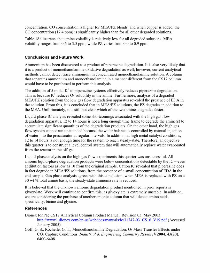
concentration. CO concentration is higher for MEA/PZ blends, and when copper is added, the CO concentration (17.4 ppm) is significantly higher than for all other degraded solutions.

Table 18 illustrates that amine volatility is relatively low for all degraded solutions. MEA volatility ranges from 0.6 to 3.5 ppm, while PZ varies from 0.0 to 0.9 ppm.

Conclusions and Future Work

Ammonium has been discovered as a product of piperazine degradation. It is also very likely that it is a product of monoethanolamine oxidative degradation as well; however, current analytical methods cannot detect trace ammonium in concentrated monoethanolamine solution. A column that separates ammonium and monoethanolamine in a manner different from the CS17 column would have to be purchased to perform this analysis.

The addition of 5 molal K+ to piperazine systems effectively reduces piperazine degradation. This is because K+ reduces O2 solubility in the amine. Furthermore, analysis of a degraded MEA/PZ solution from the low gas flow degradation apparatus revealed the presence of EDA in the solution. From this, it is concluded that in MEA/PZ solutions, the PZ degrades in addition to the MEA. Unfortunately, it is still not clear which of the two amines degrades faster.

Liquid-phase IC analysis revealed some shortcomings associated with the high gas flow degradation apparatus. 12 to 14 hours is not a long enough time frame to degrade the amine(s) to accumulate significant quantities of the degradation products. On the other hand, the high gas flow system cannot run unattended because the water balance is controlled by manual injection of water into the presaturator at regular intervals. In addition, at high metal catalyst conditions, 12 to 14 hours is not enough time for the system to reach steady-state. Therefore, an objective this quarter is to construct a level control system that will automatically replace water evaporated from the reactor in the off-gas.

Liquid-phase analysis on the high gas flow experiments this quarter was unsuccessful. All anionic liquid-phase degradation products were below concentrations detectable by the IC – even at dilution factors as low as 10 from the original sample. Cation IC revealed that piperazine does in fact degrade in MEA/PZ solutions, from the presence of a small concentration of EDA in the end sample. Gas phase analysis agrees with this conclusion; when MEA is replaced with PZ on a 30 wt % total amine basis, the steady-state ammonia rate is reduced.

It is believed that the unknown anionic degradation product mentioned in prior reports is glyoxylate. Work will continue to confirm this, as glyoxylate is extremely unstable. In addition, we are considering the purchase of another anionic column that will detect amino acids – specifically, bicine and glycine.

References Dionex IonPac CS17 Analytical Column Product Manual. Revision 03. May 2003.

http://www1.dionex.com/en-us/webdocs/manuals/ic/31747-03_CS16_V19.pdf (Accessed January 2005)

Goff, G. S., Rochelle, G. T., Monoethanolamine Degradation: O2 Mass Transfer Effects under CO2 Capture Conditions. Industrial & Engineering Chemistry Research 2004, 43(20), 6400-6408.

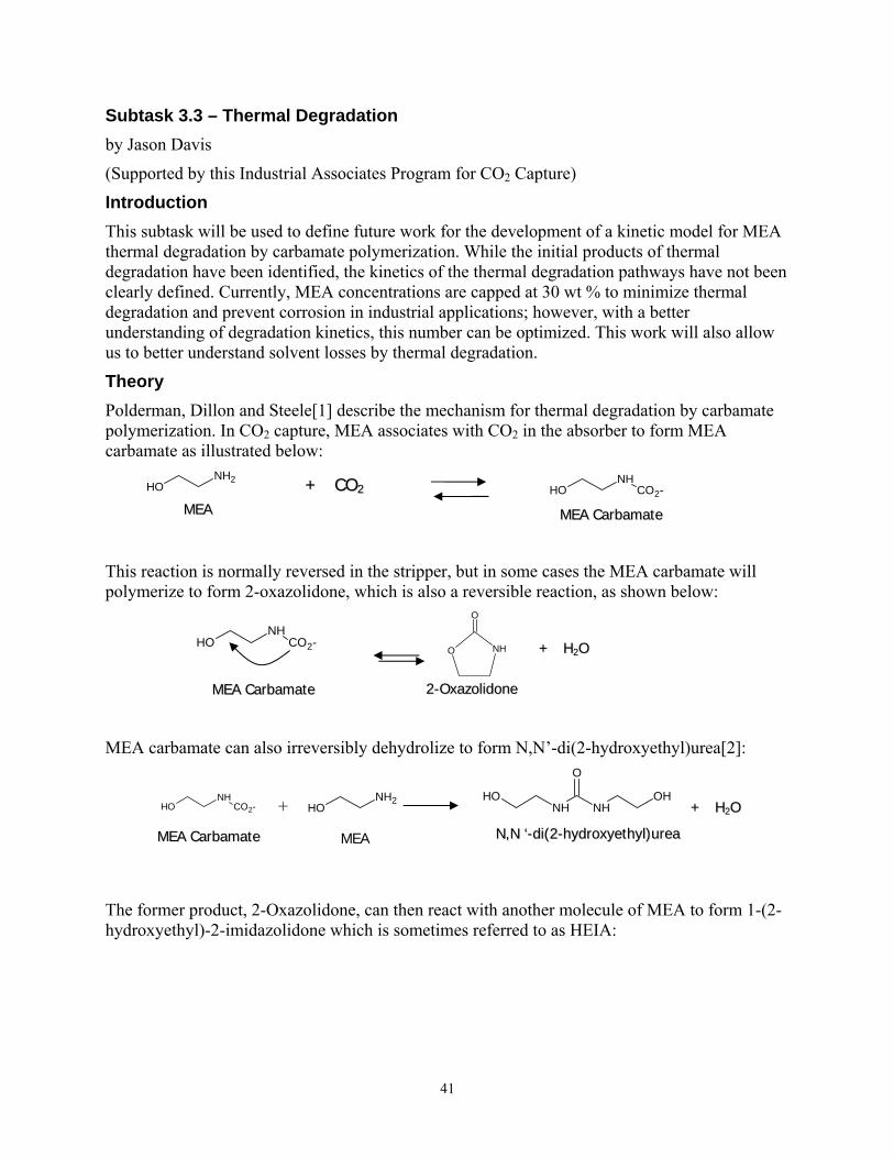
41

Subtask 3.3 – Thermal Degradation by Jason Davis

(Supported by this Industrial Associates Program for CO2 Capture)

Introduction This subtask will be used to define future work for the development of a kinetic model for MEA thermal degradation by carbamate polymerization. While the initial products of thermal degradation have been identified, the kinetics of the thermal degradation pathways have not been clearly defined. Currently, MEA concentrations are capped at 30 wt % to minimize thermal degradation and prevent corrosion in industrial applications; however, with a better understanding of degradation kinetics, this number can be optimized. This work will also allow us to better understand solvent losses by thermal degradation.

Theory Polderman, Dillon and Steele[1] describe the mechanism for thermal degradation by carbamate polymerization. In CO2 capture, MEA associates with CO2 in the absorber to form MEA carbamate as illustrated below:

This reaction is normally reversed in the stripper, but in some cases the MEA carbamate will polymerize to form 2-oxazolidone, which is also a reversible reaction, as shown below:

MEA carbamate can also irreversibly dehydrolize to form N,N’-di(2-hydroxyethyl)urea[2]:

The former product, 2-Oxazolidone, can then react with another molecule of MEA to form 1-(2-hydroxyethyl)-2-imidazolidone which is sometimes referred to as HEIA:

NH2OH

NHOH CO2-++ CCOO22

MMEEAA CCaarrbbaammaattee MMEEAA

NHO

O

22--OOxxaazzoolliiddoonnee

++ HH22OO

MMEEAA CCaarrbbaammaattee

NHOH CO2-

OHNHNH

OH

O

++ HH22OO

NN,,NN ‘‘--ddii((22--hhyyddrrooxxyyeetthhyyll))uurreeaa

NHOH CO2-

MMEEAA CCaarrbbaammaattee

NH2OH+

MEA

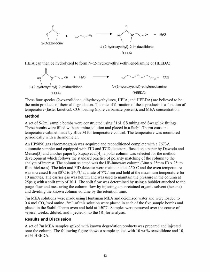
42

HEIA can then be hydrolyzed to form N-(2-hydroxyethyl)-ethylenediamine or HEEDA:

These four species (2-oxazolidone, dihydroxyethylurea, HEIA, and HEEDA) are believed to be the main products of thermal degradation. The rate of formation of these products is a function of temperature (faster kinetics), CO2 loading (more carbamate present), and MEA concentration.

Method A set of 5-2ml sample bombs were constructed using 316L SS tubing and Swagelok fittings. These bombs were filled with an amine solution and placed in a Stabil-Therm constant temperature cabinet made by Blue M for temperature control. The temperature was monitored periodically with a thermometer.

An HP5890 gas chromatograph was acquired and reconditioned complete with a 7673A automatic sampler and equipped with FID and TCD detectors. Based on a paper by Dawodu and Meisen[3] and another paper by Supap et al[4], a polar column was selected for the method development which follows the standard practice of polarity matching of the column to the analyte of interest. The column selected was the HP-Innowax column (30m x 25mm ID x 25um film thickness). The inlet and FID detector were maintained at 250oC and the oven temperature was increased from 80oC to 240oC at a rate of 7oC/min and held at the maximum temperature for 10 minutes. The carrier gas was helium and was used to maintain the pressure in the column at 25psig with a split ratio of 30:1. The split flow was determined by using a bubbler attached to the purge flow and measuring the column flow by injecting a nonretained organic solvent (hexane) and dividing the known column volume by the retention time.

7m MEA solutions were made using Huntsman MEA and deionized water and were loaded to 0.4 mol CO2/mol amine. 2mL of this solution were placed in each of the five sample bombs and placed in the Stabil-Therm oven and held at 150oC. Samples were removed over the course of several weeks, diluted, and injected onto the GC for analysis.

Results and Discussion A set of 7m MEA samples spiked with known degradation products was prepared and injected onto the column. The following figure shows a sample spiked with 10 wt % oxazolidone and 10 wt % HEEDA.

NNH

O

OH ++ HH22OO

11--((22--hhyyddrrooxxyyeetthhyyll))--22--iimmiiddaazzoolliiddoonnee

((HHEEIIAA))

NHO

O

22--OOxxaazzoolliiddoonnee

++ NH2OH

NHOH NH2 ++ CCOO22

NN--((22--hhyyddrrooxxyyeetthhyyll))--eetthhyylleenneeddiiaammiinnee

((HHEEEEDDAA))

NNH

O

OH ++ HH22OO

NNH

O

OH ++ HH22OO

11--((22--hhyyddrrooxxyyeetthhyyll))--22--iimmiiddaazzoolliiddoonnee

((HHEEIIAA))

11--((22--hhyyddrrooxxyyeetthhyyll))--22--iimmiiddaazzoolliiddoonnee

((HHEEIIAA))

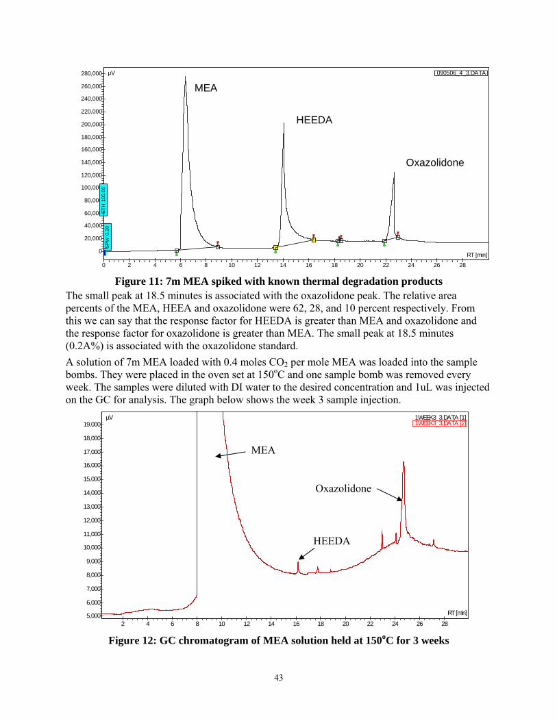
43

Figure 11: 7m MEA spiked with known thermal degradation products

The small peak at 18.5 minutes is associated with the oxazolidone peak. The relative area percents of the MEA, HEEA and oxazolidone were 62, 28, and 10 percent respectively. From this we can say that the response factor for HEEDA is greater than MEA and oxazolidone and the response factor for oxazolidone is greater than MEA. The small peak at 18.5 minutes (0.2A%) is associated with the oxazolidone standard. A solution of 7m MEA loaded with 0.4 moles CO2 per mole MEA was loaded into the sample bombs. They were placed in the oven set at 150oC and one sample bomb was removed every week. The samples were diluted with DI water to the desired concentration and 1uL was injected on the GC for analysis. The graph below shows the week 3 sample injection.

Figure 12: GC chromatogram of MEA solution held at 150oC for 3 weeks

282624222018161412108642

19,000

18,000

17,000

16,000

15,000

14,000

13,000

12,000

11,000

10,000

9,000

8,000

7,000

6,000

5,000 RT [min]

1WEEK3_3.DATA [1]1WEEK3_3.DATA [2]

µV

2826242220181614121086420

280,000

260,000

240,000

220,000

200,000

180,000

160,000

140,000

120,000

100,000

80,000

60,000

40,000

20,000

0

SP

W 0

.20

ST

H 1

00.0

0

RT [min]

090506_4_3.DATAµV

MEA

HEEDA

Oxazolidone

MEA

Oxazolidone

HEEDA

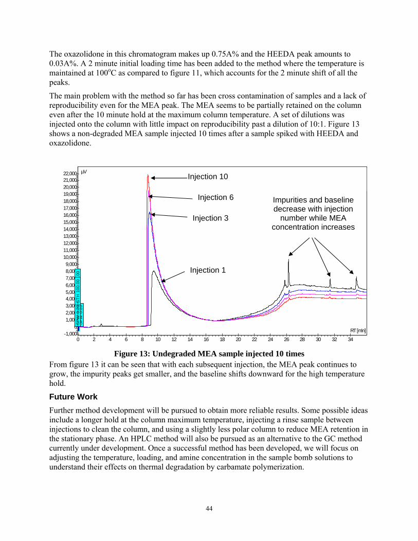
44

The oxazolidone in this chromatogram makes up 0.75A% and the HEEDA peak amounts to 0.03A%. A 2 minute initial loading time has been added to the method where the temperature is maintained at 100oC as compared to figure 11, which accounts for the 2 minute shift of all the peaks.

The main problem with the method so far has been cross contamination of samples and a lack of reproducibility even for the MEA peak. The MEA seems to be partially retained on the column even after the 10 minute hold at the maximum column temperature. A set of dilutions was injected onto the column with little impact on reproducibility past a dilution of 10:1. Figure 13 shows a non-degraded MEA sample injected 10 times after a sample spiked with HEEDA and oxazolidone.

Figure 13: Undegraded MEA sample injected 10 times

From figure 13 it can be seen that with each subsequent injection, the MEA peak continues to grow, the impurity peaks get smaller, and the baseline shifts downward for the high temperature hold.

Future Work Further method development will be pursued to obtain more reliable results. Some possible ideas include a longer hold at the column maximum temperature, injecting a rinse sample between injections to clean the column, and using a slightly less polar column to reduce MEA retention in the stationary phase. An HPLC method will also be pursued as an alternative to the GC method currently under development. Once a successful method has been developed, we will focus on adjusting the temperature, loading, and amine concentration in the sample bomb solutions to understand their effects on thermal degradation by carbamate polymerization.

3432302826242220181614121086420

22,00021,00020,00019,00018,00017,00016,00015,00014,00013,00012,00011,00010,0009,0008,0007,0006,0005,0004,0003,0002,0001,000

0-1,000

SPW

0.2

0S

TH 1

00.0

0SP

W 0

.20

STH

100

.00

SPW

0.2

0S

TH 1

00.0

0SP

W 0

.20

STH

100

.00

RT [min]

MEA1_1.DATAMEA1_10.DATAMEA1_3.DATAMEA1_6.DATA

µVInjection 10

Injection 6

Injection 3

Injection 1

Impurities and baseline decrease with injection

number while MEA concentration increases

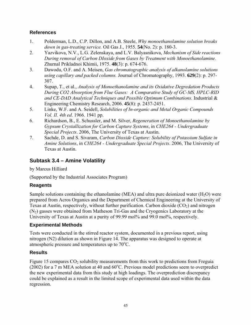
45

References

1. Polderman, L.D., C.P. Dillon, and A.B. Steele, Why monoethanolamine solution breaks down in gas-treating service. Oil Gas J., 1955. 54(No. 2): p. 180-3.

2. Yazvikova, N.V., L.G. Zelenskaya, and L.V. Balyasnikova, Mechanism of Side reactions During removal of Carbon DIoxide from Gases by Treatment with Monoethanolamine. Zhurnal Prikladnoi Khimii, 1975. 48(3): p. 674-676.

3. Dawodu, O.F. and A. Meisen, Gas chromatographic analysis of alkanolamine solutions using capillary and packed columns. Journal of Chromatography, 1993. 629(2): p. 297-307.

4. Supap, T., et al., Analysis of Monoethanolamine and its Oxidative Degredation Products During CO2 Absorption from Flue Gases: A Comparative Study of GC-MS, HPLC-RID and CE-DAD Analytical Techniques and Possible Optimum Combinations. Industrial & Engineering Chemistry Research, 2006. 45(8): p. 2437-2451.

5. Linke, W.F. and A. Seidell, Solubilities of In-organic and Metal Organic Compounds Vol. II. 4th ed. 1966. 1941 pp.

6. Richardson, B., E. Schussler, and M. Silver, Regeneration of Monoethanolamine by Gypsum Crystallization for Carbon Capture Systems, in CHE264 - Undergraduate Special Projects. 2006, The University of Texas at Austin.

7. Sachde, D. and S. Sivaram, Carbon Dioxide Capture: Solubility of Potassium Sulfate in Amine Solutions, in CHE264 - Undergraduate Special Projects. 2006, The University of Texas at Austin.

Subtask 3.4 – Amine Volatility by Marcus Hilliard

(Supported by the Industrial Associates Program)

Reagents

Sample solutions containing the ethanolamine (MEA) and ultra pure deionized water (H2O) were prepared from Acros Organics and the Department of Chemical Engineering at the University of Texas at Austin, respectively, without further purification. Carbon dioxide (CO2) and nitrogen (N2) gasses were obtained from Matheson Tri-Gas and the Cryogenics Laboratory at the University of Texas at Austin at a purity of 99.99 mol% and 99.0 mol%, respectively.

Experimental Methods Tests were conducted in the stirred reactor system, documented in a previous report, using nitrogen (N2) dilution as shown in Figure 14. The apparatus was designed to operate at atmospheric pressure and temperatures up to 70oC.

Results

Figure 15 compares CO2 solubility measurements from this work to predictions from Freguia (2002) for a 7 m MEA solution at 40 and 60oC. Previous model predictions seem to overpredict the new experimental data from this study at high loadings. The overprediction discrepancy could be explained as a result in the limited scope of experimental data used within the data regression.

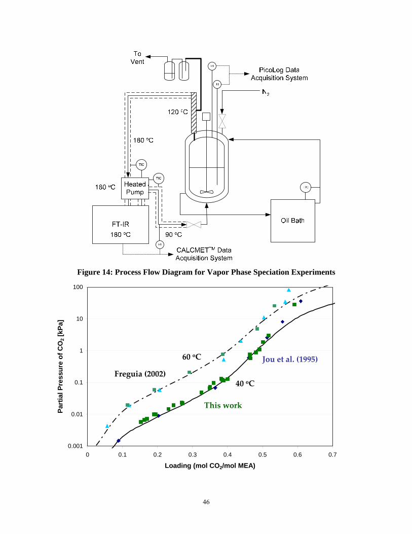
46

Figure 14: Process Flow Diagram for Vapor Phase Speciation Experiments

0.001

0.01

0.1

1

10

100

0 0.1 0.2 0.3 0.4 0.5 0.6 0.7

Loading (mol CO2/mol MEA)

Part

ial P

ress

ure

of C

O2 [

kPa]

This work

Freguia (2002)

Jou et al. (1995)60 oC

40 oC

47

Figure 15: Comparison of CO2 solubility results from this work and Jou et al. (1995) to predictions from Freguia (2002) at 40 and 60oC

Future work Work will continue to quantify the CO2 solubility and amine volatility for 3.5, 7, and 11 m MEA.

Conclusions Our research has been able to benchmark our experimental apparatus for measurement CO2 solubility against literature data. We are now confident in our approach and will continue our efforts in this area.

Task 5 – Corrosion Subtask 5.1 – Corrosion in base solution compared to MEA by Amornvadee (Amy) Veawab, University of Regina

Supported by subcontract

Introduction

The carbon dioxide (CO2) absorption process using aqueous chemical solutions is subject to a number of operational difficulties, of which the most severe is corrosion of process equipment and solvent degradation. Corrosion problems have been receiving a great deal of attention because they have substantial impacts on the plant’s economy, especially in terms of unplanned downtime, production losses, reduced equipment life, and extra expenditure for restoring the corroded equipment and for treatment systems initiated to mitigate the corrosion. The corrosion problems also prevent the absorption process from achieving energy efficient operations.

The aqueous solution of blended potassium carbonate and piperazine has been demonstrated to be a promising solvent for CO2 capture from coal-fired power plant flue gas due to its capture performance and energy efficiency. It is our goal to further explore the promise of this solvent in an aspect of the potential operational problems. This project focuses on the investigation of corrosion of materials during CO2 absorption and solvent regeneration in the presence and absence of solvent degradation products and chemical additives including oxidative inhibitors and corrosion inhibitors.

The research involves comprehensive literature review on the corrosion in CO2 absorption process using potassium carbonate and piperazine, and experimental evaluations in the following sequences:

Task 1: Evaluation of corrosion in base solution (the blended potassium carbonate and piperazine) against the corrosion in an aqueous solution of monoethanolamine (MEA).

Task 2: Evaluation of corrosion in base solution containing degradation products.

Task 3: Evaluation of corrosion in base solution containing degradation products and oxidative inhibitors.

Task 4: Evaluation of inhibition performance of corrosion inhibitor in the presence of degradation products and oxidative inhibitors.

48

Based on our discussion with Dr. Rochelle, we would like to expand our project to cover the corrosion study in both K2CO3-piperazine and MEA-piperazine since MEA-piperazine is another promising piperazine-based solvent for the cost-effective CO2 capture. The original tasks for K2CO3-MEA will be kept minimum, and the tasks with similar objectives will be carried out for MEA-piperazine system.

Results Over the past three months, we have been conducting a series of short-term electrochemical corrosion experiments under various conditions to obtain corrosion rate of carbon steel and gain understanding of corrosion behavior in aqueous solutions of MEA and blended MEA-piperazine. Results and discussion are provided below.

Effect of temperature The effect of temperature was studied at 40 and 80ºC using an aqueous solution of 7m MEA-1.7m piperazine containing 0.20 mol/mol CO2 loading. The cyclic polarization curves (Figure 16) reveal that as the solution temperature increases, the entire polarization curve shifts to the right where rates of iron dissolution and oxidizing agent reduction are enhanced. No changes in anodic and cathodic Tafel slopes, and no pitting tendency are observed. This indicates that the corrosion rate increases with temperature without an alteration of corrosion mechanism. As shown in Figure 17, the corrosion rate of carbon steel increases from 33 to 63 mpy when the solution temperature increases from 40 to 80oC.

Effect of heat-stable salts Three types of heat-stable salts, formate, acetate, and oxalate, were chosen in our test program since they were reported to increase the corrosion rates in MEA and MDEA systems. These salts were added as acid anions (i.e., formic acid, acetic acid, and oxalic acid) to an aqueous solution of 5m MEA-1.2 m piperazine with the concentration of 1% wt. The results (Figures 18-21) clearly indicate that these three salts make the MEA-piperazine solution more corrosive in both presence and absence of dissolved oxygen. In the presence of dissolved oxygen, acetate is the most corrosive, followed by formate and oxalate. However, the difference trend of corrosion rate is found in the system without dissolved oxygen. Formate and acetate appear to significantly increase the corrosion rate to a comparable value, while oxalate induces much less with an evidence of pitting tendency.

Effect of piperazine concentration (mixing ratio) The effect of piperazine concentration or mixing the ratio of MEA and piperazine was investigated in aqueous solutions of MEA and blended MEA-piperazine with the total concentration of 6.2 m containing 0.20 mol/mol CO2 loading at 80oC. The results (Figures 22-23) indicate that piperazine is more corrosive than MEA. The corrosion rate of carbon steel increases with increasing piperazine concentration. The corrosion rate in the system with the mixing ratio of 1:1 (3.1m MEA-3.1 m piperazine) is extremely high (181 mpy), while that in 6.2m MEA is only 19.23 mpy, and that of the mixing ratio of 4:1 (5 m MEA-1.2 m PZ) is 21.79 mpy.

Effect of dissolved oxygen The effect of dissolved oxygen was studied by using an aqueous solution of 5 m MEA-1.2 m piperazine containing 0.20 mol/mol CO2 loading and 5% oxygen in gas. The polarization curves

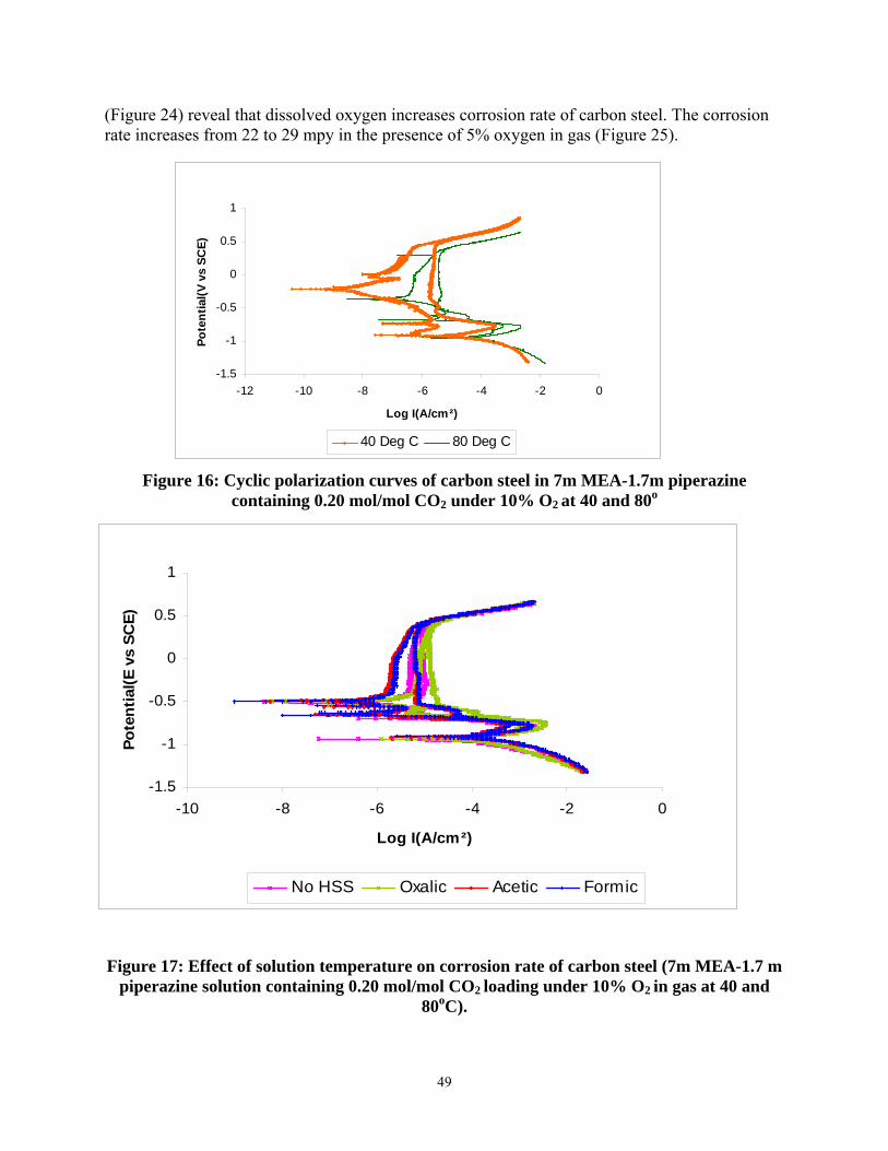
49

(Figure 24) reveal that dissolved oxygen increases corrosion rate of carbon steel. The corrosion rate increases from 22 to 29 mpy in the presence of 5% oxygen in gas (Figure 25).

Figure 16: Cyclic polarization curves of carbon steel in 7m MEA-1.7m piperazine containing 0.20 mol/mol CO2 under 10% O2 at 40 and 80o

Figure 17: Effect of solution temperature on corrosion rate of carbon steel (7m MEA-1.7 m

piperazine solution containing 0.20 mol/mol CO2 loading under 10% O2 in gas at 40 and 80oC).

-1.5

-1

-0.5

0

0.5

1

-12 -10 -8 -6 -4 -2 0

Log I(A/cm²)

Pote

ntia

l(V v

s SC

E)

40 Deg C 80 Deg C

-1.5

-1

-0.5

0

0.5

1

-10 -8 -6 -4 -2 0

Log I(A/cm²)

Pote

ntia

l(E v

s SC

E)

No HSS Oxalic Acetic Formic

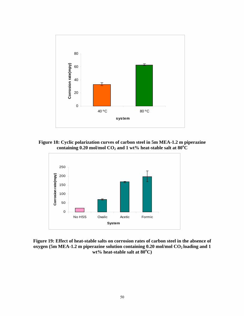
50

Figure 18: Cyclic polarization curves of carbon steel in 5m MEA-1.2 m piperazine containing 0.20 mol/mol CO2 and 1 wt% heat-stable salt at 80oC

Figure 19: Effect of heat-stable salts on corrosion rates of carbon steel in the absence of oxygen (5m MEA-1.2 m piperazine solution containing 0.20 mol/mol CO2 loading and 1

wt% heat-stable salt at 80oC)

0

20

40

60

80

40 ºC 80 ºC

system

Cor

rosi

on ra

te(m

py)

0

50

100

150

200

250

No HSS Oxalic Acetic Formic

System

Cor

rosi

on ra

te(m

py)

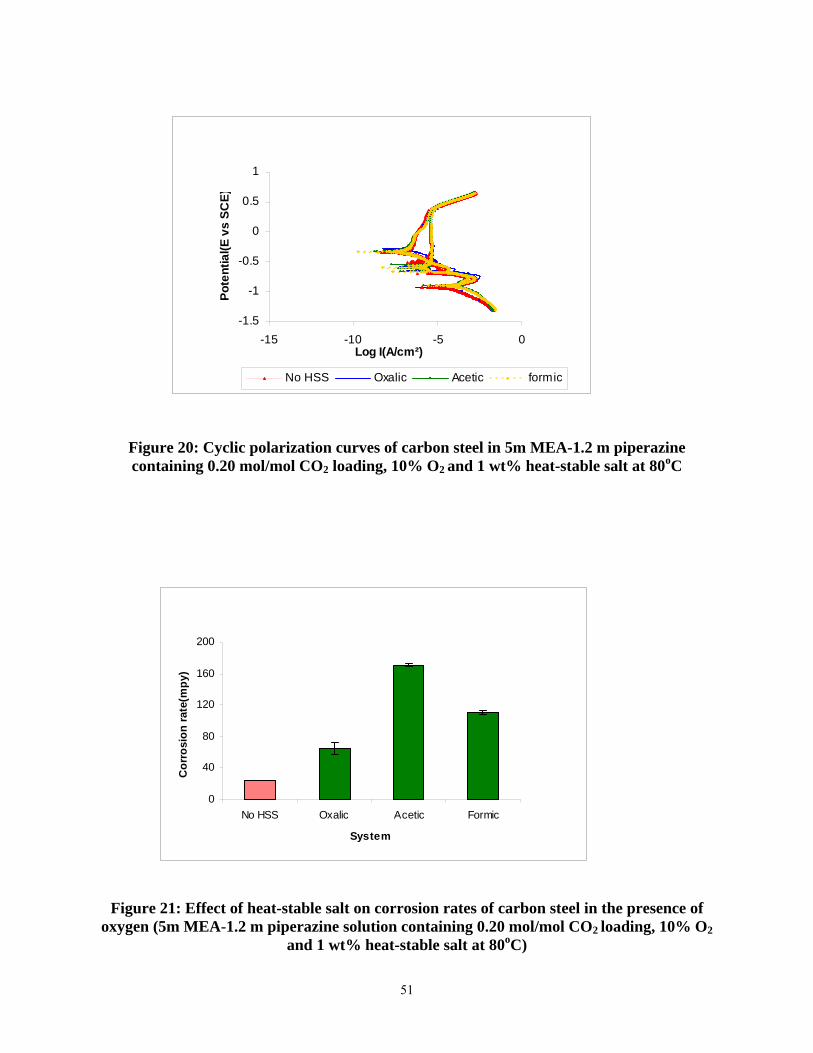
51

Figure 20: Cyclic polarization curves of carbon steel in 5m MEA-1.2 m piperazine containing 0.20 mol/mol CO2 loading, 10% O2 and 1 wt% heat-stable salt at 80oC

Figure 21: Effect of heat-stable salt on corrosion rates of carbon steel in the presence of oxygen (5m MEA-1.2 m piperazine solution containing 0.20 mol/mol CO2 loading, 10% O2

and 1 wt% heat-stable salt at 80oC)

-1.5

-1

-0.5

0

0.5

1

-15 -10 -5 0Log I(A/cm²)

Pote

ntia

l(E v

s SC

E)

No HSS Oxalic Acetic formic

0

40

80

120

160

200

No HSS Oxalic Acetic Formic

System

Cor

rosi

on ra

te(m

py)

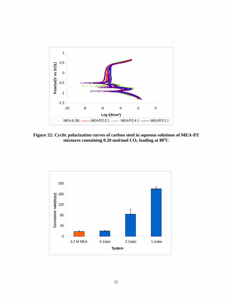
52

Figure 22: Cyclic polarization curves of carbon steel in aqueous solutions of MEA-PZ mixtures containing 0.20 mol/mol CO2 loading at 80oC

-1.5

-1

-0.5

0

0.5

1

-10 -8 -6 -4 -2 0

Log I(A/cm²)

Pot

etia

l(V v

s S

CE)

MEA-6.2M MEA/PZ-2:1 MEA/PZ-4:1 MEA/PZ-1:1

0

40

80

120

160

200

6.2 M MEA 4:1ratio 2:1ratio 1:1ratio

System

Corr

osio

n ra

te(m

py)

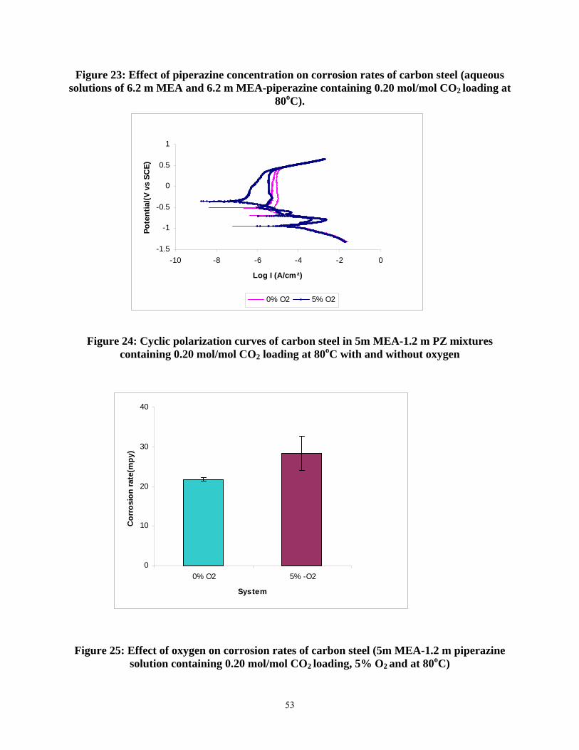
53

Figure 23: Effect of piperazine concentration on corrosion rates of carbon steel (aqueous solutions of 6.2 m MEA and 6.2 m MEA-piperazine containing 0.20 mol/mol CO2 loading at

80oC).

Figure 24: Cyclic polarization curves of carbon steel in 5m MEA-1.2 m PZ mixtures containing 0.20 mol/mol CO2 loading at 80oC with and without oxygen

Figure 25: Effect of oxygen on corrosion rates of carbon steel (5m MEA-1.2 m piperazine solution containing 0.20 mol/mol CO2 loading, 5% O2 and at 80oC)

-1.5

-1

-0.5

0

0.5

1

-10 -8 -6 -4 -2 0

Log I (A/cm²)

Pote

ntia

l(V v

s SC

E)

0% O2 5% O2

0

10

20

30

40

0% O2 5% -O2

System

Cor

rosi

on ra

te(m

py)

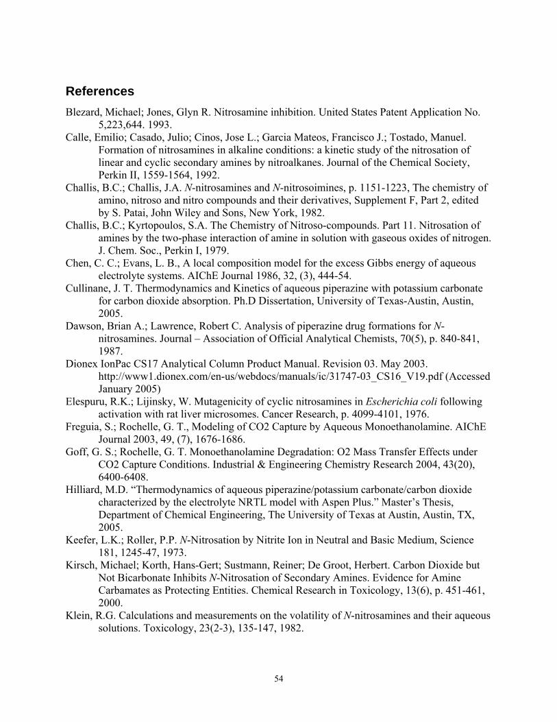
54

References Blezard, Michael; Jones, Glyn R. Nitrosamine inhibition. United States Patent Application No.

5,223,644. 1993. Calle, Emilio; Casado, Julio; Cinos, Jose L.; Garcia Mateos, Francisco J.; Tostado, Manuel.

Formation of nitrosamines in alkaline conditions: a kinetic study of the nitrosation of linear and cyclic secondary amines by nitroalkanes. Journal of the Chemical Society, Perkin II, 1559-1564, 1992.

Challis, B.C.; Challis, J.A. N-nitrosamines and N-nitrosoimines, p. 1151-1223, The chemistry of amino, nitroso and nitro compounds and their derivatives, Supplement F, Part 2, edited by S. Patai, John Wiley and Sons, New York, 1982.

Challis, B.C.; Kyrtopoulos, S.A. The Chemistry of Nitroso-compounds. Part 11. Nitrosation of amines by the two-phase interaction of amine in solution with gaseous oxides of nitrogen. J. Chem. Soc., Perkin I, 1979.

Chen, C. C.; Evans, L. B., A local composition model for the excess Gibbs energy of aqueous electrolyte systems. AIChE Journal 1986, 32, (3), 444-54.

Cullinane, J. T. Thermodynamics and Kinetics of aqueous piperazine with potassium carbonate for carbon dioxide absorption. Ph.D Dissertation, University of Texas-Austin, Austin, 2005.

Dawson, Brian A.; Lawrence, Robert C. Analysis of piperazine drug formations for N-nitrosamines. Journal – Association of Official Analytical Chemists, 70(5), p. 840-841, 1987.

Dionex IonPac CS17 Analytical Column Product Manual. Revision 03. May 2003. http://www1.dionex.com/en-us/webdocs/manuals/ic/31747-03_CS16_V19.pdf (Accessed January 2005)

Elespuru, R.K.; Lijinsky, W. Mutagenicity of cyclic nitrosamines in Escherichia coli following activation with rat liver microsomes. Cancer Research, p. 4099-4101, 1976.

Freguia, S.; Rochelle, G. T., Modeling of CO2 Capture by Aqueous Monoethanolamine. AIChE Journal 2003, 49, (7), 1676-1686.

Goff, G. S.; Rochelle, G. T. Monoethanolamine Degradation: O2 Mass Transfer Effects under CO2 Capture Conditions. Industrial & Engineering Chemistry Research 2004, 43(20), 6400-6408.

Hilliard, M.D. “Thermodynamics of aqueous piperazine/potassium carbonate/carbon dioxide characterized by the electrolyte NRTL model with Aspen Plus.” Master’s Thesis, Department of Chemical Engineering, The University of Texas at Austin, Austin, TX, 2005.

Keefer, L.K.; Roller, P.P. N-Nitrosation by Nitrite Ion in Neutral and Basic Medium, Science 181, 1245-47, 1973.

Kirsch, Michael; Korth, Hans-Gert; Sustmann, Reiner; De Groot, Herbert. Carbon Dioxide but Not Bicarbonate Inhibits N-Nitrosation of Secondary Amines. Evidence for Amine Carbamates as Protecting Entities. Chemical Research in Toxicology, 13(6), p. 451-461, 2000.

Klein, R.G. Calculations and measurements on the volatility of N-nitrosamines and their aqueous solutions. Toxicology, 23(2-3), 135-147, 1982.

55

Linke, W.F., Seidell, A., Solubilities, Inorganic and Metal-Organic Comounds, D. Van Nostrad Company Inc., Princeton, NJ, 1958.

Love, L.A.; Lijinsky, W.; Keefer, L.; Garcia, H. Chronic oral administration of 1-nitrosopiperazine in high doses to MRC rats. Z. Krebsforsch., p. 69-73, 1977.

Lovejoy, D.J.; Vosper, A.J. Part VI. The Reaction of Dinitrogen Trioxide with Primary and Secondary Amines, J. Chem. Soc. (A), 2325-2328, 1968.

Mock, B.; Evans, L. B.; Chen, C. C., Thermodynamic representation of phase equilibria of mixed-solvent electrolyte systems. AIChE Journal 1986, 32, (10), 1655-64.

Onda, K.; Takeuchi, H.; Okumoto, Y., Mass transfer coefficients between gas and liquid phases in packed columns. Journal of Chemical Engineering of Japan 1968, 1, (1), 56-62.

Oyenekan, B. A.; Rochelle, G. T., Energy Performance of Stripper Configurations for CO2 Capture by Aqueous Amines. Ind Eng Chem Res 2006, 45, (8), 2457-64.

Oyenekan, B. A.; Rochelle, G. T., Alternative Stripper Configurations to Minimize Energy for CO2 Capture. In 8th International Conference on Greenhouse Gas Control Technologies, Trondheim,Norway, 2006.

Richardson, B., Schussler, E., and Silver, M., “Regeneration of Monoethanolamine by Gypsum Crystallization for Carbon Capture Systems”, University of Texas - CHE 264 Undergraduate Special Project, Spring 2006.

Rochelle, G. T. Personal Communication to Andrew Sexton. Austin, TX, 2005. Sachde, D., and Sivaram, S., “CO2 Capture: Solubility of Potassium Sulfate in Amine Solutions”,

University of Texas - CHE 264 Undergraduate Special Project, Summer 2006 Shoulders, B. Personal Communication to Andrew Sexton. Austin, TX, 2005. Smith, P.A.S.; Loeppky, R.N. Nitrosative Cleavage of Tertiary Amines, J, ACS, 89, 1147-1157,

1967. Talzi, V.P., “NMR Determination of the Total Composition of Commercial Absorbents Based on

Monoethanolamine”, Russian Journal of Applied Chemistry, 2004, 77(3), 437-441. Tobiesen, F. A.; Svendsen, H. F.; Hoff, K. A., Desorber energy consumption in amine based

absorption plants. Int. J of Green Energy 2005, 2, 1-15. Tricker, A.R.; Kumar, R.; Siddiqi, M.; Khuroo, M.S.; Preusmann, R. Endogenous formation of

N-nitrosamines from piperazine and their urinary excretion following antihelmintic treatment with piperazine citrate. Carcinogenesis, 12(9), p. 1595-1599, 1991.

Wang, J. Personal Communication to Andrew Sexton. Austin, TX, 2005. Weiland, R. H.; Rawal, M.; Rice, R. G., Stripping of carbon dioxide from monoethanolamine

solutions in a packed column. AIChE Journal 1982, 28, (6), 963-73.