CNOIDAL WAVE FORMATION IN A LASER SYSTEM WITH …biblioteca.cio.mx/tesis/15032.pdf · on horseback, and overtook it still rolling on at a rate of some eight or nine miles an hour

CNOIDAL WAVE FORMATION IN A LASER SYSTEM

WITH ACTIVE SATURABLE ABSORBER

By:

Mario César Wilson Herrán, M. S.

Dissertation presented in partial fulfillment

of the requirements for the degree of

Doctor of Philosophy

in

Optics

Advisor

Dr. Vicente Aboites

León, Gto. México

August 2011

Final version.

“Include all the suggestions and comments made by the thesis reviewers”

___________________

Dr. Vicente Aboites

Thesis supervisor

León, Gto. August 22, 2011

ABSTRACT

0

ABSTRACT

We demonstrate the cnoidal wave formation in a two-laser system with a saturable

absorber inside the cavity of one of the lasers. The other laser is used to activate the

saturable absorber in order to control the pulse shape, width, intensity and frequency.

The direct modulation enables to control when and how the pulse train coming from the

saturable absorber is released. Using a three-level laser model rate equations based on

the Statz – de Mars model, we show that for any value of saturable absorber parameter

there exist a certain modulation frequency for which the pulse shape is very close to a

soliton shape with less than 5% error at the pulse base. Such a device may be prominent

for optical communication and laser engineering applications.

RESUMEN

Demostramos la formación de ondas cnoidales en un sistema de dos láseres con un

absorbedor saturable dentro de la cavidad de uno de ellos. El otro láser es utilizado para

activar al absorbedor saturable y así poder controlar la forma, el ancho, la intensidad y

la frecuencia de los pulsos generados. La modulación directa permite controlar cuándo

y cómo se libera el tren de pulsos que proviene del absorbedor saturable. Usando un

modelo de ecuaciones de balance para un láser de tres niveles basados en el modelo de

Statz – de Mars, demostramos que para cualquier valor de parámetro del absorbedor

saturable existe cierta frecuencia de modulación con la que la forma del pulso generado

es muy cercana a la forma de un solitón con menos del 5% de error en la base del pulso.

Dicho dispositivo puede ser prominente para comunicaciones ópticas y aplicaciones de

ingeniería láser.

I

To my Family. . .

II

ACKNOWLEDGMENTS

I would like to thank Dr. Vicente Aboites for his patience, support and

encouragement in my research. I greatly appreciate the latitude I was given in

pursuing the research contained in this dissertation. The lessons I learned in the

approach to research will serve me well during the rest of my research career.

I would also like to thank Dr. Alexander Pisarchik for countless discussions which

helped inspire the work contained in this thesis. His help in organizing my thoughts

on solitons and dynamics is specially appreciated.

I would like to thank the other members of my committee, Dr. Bernardo Mendoza,

Dr. Flavio Ruiz-Oliveras, Dr. Victor Pinto, Dr. Rider Jaimes-Reategui and Dr.

Ismael Torres. Likewise, I especially remember Dr. Mendoza for his great

comments on the Lyapunov seminar.

Furthermore, I want to thank Dr. Majid Taki and Dr. Saliya Coulibaly, for all the

knowledge, patience and good moments in Lille, France.

I thank to all the people that directly or indirectly have something to do with this

work, to the project No. M08P02 between ANUIES CONACyT – ECOS for

providing me the opportunity to make two short stays in Lille, France, to the

Instituto Euroamericano for the logistic support in some congresses and, especially,

to the CONACyT for giving me financial support through the grant No. 174725.

I want to also thank my family as well as all my friends for their support in this

quest. Thanks to my mother and father for helping me and motivating me to make it

to where I am today.

III

Finally, I would like to thank my wife Linda. She has stood by me through all these

years of my doctoral study with love, patience, support and great friendship. I will

always cherish these years during which we grew together and fell in love. Thank

you.

MARIO CÉSAR WILSON HERRÁN Centro de Investigaciones en Óptica, A.C.

August 2011

IV

INDEX

V

CONTENT

INDEX…………………………………………………………………….……………..…V

FIGURES LIST………………..………………………………………….……………..VIII

THESIS GENERAL OVERVIEW…………………….………………………..…………XI

CHAPTER 1

PRELIMINARIES

1.0 INTRODUCTION..…………………………………………………..….................1

1.1 SOLITONS……..………………………..…………………………….………….…1

1.2 ELLIPTIC FUNCTIONS.…………………………………………………………...7

1.3 CNOIDAL WAVE….………..………………………………………………….…..9

1.4 RATE EQUATIONS……………………………………………………….………11

1.4.1 RATE EQUATIONS IN ABSENCE OF AMPLIFIER RADIATION........13

1.4.2 RATE EQUATIONS IN PRESENCE OF AMPLIFIER RADIATION…...14

1.5 STATZ – DE MARS MODEL…………………………………………………......15

1.6 SATURABLE ABSORBERS……………………………………………………...17

FIRST CHAPTER REFERENCES………………………………………………………..18

INDEX

VI

CHAPTER 2

THEORETICAL MODEL

2.0 INTRODUCTION………….…………………………………………………........20

2.1 LASER SCHEME………………………………………………………………….20

2.2. LASER MODEL…………………………………………………………………...21

2.3 LINEAR STABILITY ANALYSIS……………………………………................27

SECOND CHAPTER REFERENCES…………………………………………………….32

CHAPTER 3

RESULTS AND CONCLUSIONS

3.0 INTRODUCTION………………………………………………………………….34

3.1 CONTROLLING THE SYSTEM DYNAMICS…………………………………...34

3.2 CNOIDAL WAVE OBSERVATION……………………………………………...40

3.3 CONCLUSIONS…………………………………………………………………...44

3.4 FUTURE WORK…………………………..………………………………………45

THIRD CHAPTER REFERENCES……………………………………………………….47

INDEX

VII

APPENDIX 1

LIST OF PUBLICATIONS

A1.1 PEER-REVIEWED INDEXED JOURNALS………………………………………..i

A1.2 CONFERENCES……………………………………………………………………ii

FIGURES LIST

VIII

FIGURES LIST

CHAPTER 1 PRELIMINARIES

Figure 1 Russell’s scheme of his studies about the “wave of translation”

Figure 2 A solitary wave travelling to the beach in a Hawaiian isle.

Figure 3 Light bullets interaction, when these type of soliton interact they lose

certain quantity of energy.

Figure 4 Argand diagram constructed to show the formation of the Jacobi

elliptic functions

Figure 5 Cnoidal wave profile achieve for different parameter’s value.

Figure 6 Cnoidal wave limits. a)sinusoidal shape. b) soliton shape.

Figure 7 Two energy levels diagram including life-times

Figure 8 Energy levels 1 and 2 with surrounding higher and lower energy

levels

Figure 9 The population densities N1 and N2 (cm-3s-1) of atoms in energy

levels 1 and 2 are determined by three processes: decay (b),

pumping(r), and absorption and stimulated emission (g)

FIGURES LIST

IX

CHAPTER 2 THEORETICAL MODEL

Figure 10 Optical scheme for a laser system with an active saturable absorber.

AM and SA are active medium and saturable absorber, M1 and M2 are

total reflected and semi-transparent laser mirrors, and EOM is an

electro-optical modulator.

Figure 11 A laser cavity with an active medium and a saturable absorber.

Figure 12 Stability condition given by the relation between α and αα.

CHAPTER 3 RESULTS AND CONCLUSIONS

Figure 13 Laser output without external modulation, the system tends to a fixed

point.

Figure 14 Laser output with fixed modulation (ω = 1) and variable absorption

ratio. a) αα = 0.3, b) αα = 1, c) αα = 3, d) αα = 15, e) αα = 30 and f)

αα = 60.

Figure 15 Phase diagram m vs na. a) with αa = 1.4 b)with αa = 30.

Figure 16 Pulse shape at αa = 15 with different frequencies a) ω = 1/4,

b) ω = 1/2, c) ω = 2, d) ω = 5, e) ω = 10, f) ω = 35.

Figure 17 Pulse width against control frequency. It is shown how the pulses

width become narrower as the control frequency is increased.

Figure 18 Laser output intensity for αa = 15 and control frequencies (a) ω = 1,

(b) 5, (c) 15, (d) 25, (e) 50, and (f) 75.

FIGURES LIST

X

Figure 19 Overlapping of one pulse taken at αa = 15 and ω = 25 (solid line)

with a sech2 wave form (dashed line).

Figure 20 Modulation frequency ωs and absorption ratio of saturable absorber

corresponding to soliton-shape pulses.

Figure 21 Experimental set-up implemented for search cnoidal waves.

Figure 22 Experimental cnoidal wave limits. a) soliton-shape limit,

b) sinusoidal shape limit.

THESIS GENERAL OVERVIEW

XI


This thesis presents the study of a laser with an active saturable absorber by means of

the rate equations; the main objective is to produce cnoidal waves through controlling

the laser dynamics.

The thesis is composed by three chapters that are organized as follows

Chapter 1: Preliminaries

In this chapter the elemental concepts needed to have a better understanding

of the work are boarded. The chapter contemplates subjects as solitons, elliptic

functions, rate equations, cnoidal waves and saturable absorbers.

Chapter 2: Theoretical model

In this chapter, the experiment proposal is presented, with the aid of the rate

equations. A model for the experiment is proposed and its linear stability analysis is

done in order to know the fixed points of the system and its stability.

Chapter 3: Results and conclusions

In this part of the thesis, the obtained results are presented; the chapter

contains the dynamics control and the cnoidal waves observation. At the end of the


XII

chapter, the conclusions are followed by a future work proposal (some preliminaries

results have been obtained).

As an appendix there is a list of publications made during the doctoral studies.

1. PRELIMINARIES

1

CHAPTER 1

PRELIMINARIES

1.0.INTRODUCTION

In this chapter a basic introduction to the matters dealt in this dissertation are presented

in order to have a better understanding of the results discussed in this dissertation.

1.1. SOLITONS

The first natural definition that comes to mind when the word soliton is heard reefers to

a self-reinforcing solitary wave that does not have variation on its shape while it is

traveling along a media at a constant speed.

These kinds of waves are caused by compensation (cancellation) between the nonlinear

(e.g. Kerr and Raman effects in fiber optics) and the dispersive effects of the

propagating medium. Solitons exist as a solution of many weakly nonlinear dispersive

partial differential equations, used to describe different physical phenomena [1].

In 1844, John Scott Russell reported the observation of a solitary wave [2] in the Union

Canal, Scotland, while he was doing some experiments to determine the most efficient

design for canal boats. He called that phenomenon wave of translation, and by his own

words it was described as follows:

1. PRELIMINARIES

2

―I was observing the motion of a boat which was rapidly drawn along a narrow

channel by a pair of horses, when the boat suddenly stopped—not so the mass of

water in the channel which it had put in motion; it accumulated round the prow of

the vessel in a state of violent agitation, then suddenly leaving it behind, rolled

forward with great velocity, assuming the form of a large solitary elevation, a

rounded, smooth and well-defined heap of water, which continued its course along

the channel apparently without change of form or diminution of speed. I followed it

on horseback, and overtook it still rolling on at a rate of some eight or nine miles an

hour [14 km/h], preserving its original figure some thirty feet [9 m] long and a foot

to a foot and a half [300−450 mm] in height. Its height gradually diminished, and

after a chase of one or two miles [2–3 km] I lost it in the windings of the channel.

Such, in the month of August 1834, was my first chance interview with that singular

and beautiful phenomenon which I have called the Wave of Translation.‖

Russell spent a lot of time trying to repeat and understand these kinds of waves (see

Fig. 1); after several tries he found some properties:

- The waves are stable in long distances.

- The speed depends on the wave’s amplitude and the wave’s width on the deepness

of the water.

- They never merge between them.

- If the medium can’t contain a big wave due the water depth, the wave splits into

two, one bigger than the other.

Despite of Russell’s founds, the scientific community didn’t accept his discoveries due

to the contrast with the Newton and Bernoulli theories of hydrodynamics.

1. PRELIMINARIES

3

FIGURE 1. Russell’s scheme of his studies about the ―wave of translation‖

The problem was theoretically unexplained until 1876, when Lord Rayleigh published a

paper in the ―Philosophical Magazine‖ supporting Russell’s experimental observation.

In that paper, Lord Rayleigh presented his mathematical theory [3] and mentioned that

the first theoretical treatment was made by Joseph Boussinesq five years earlier [4]

(Boussinesq also cited Russell in his work). Twenty years later, Korteweg and de Vries

published a paper called ―On the change of form of long waves advancing in a

rectangular canal and on a new type of long stationary waves‖ also in the

1. PRELIMINARIES

4

―Philosophical Magazine‖ [5], in this work they didn’t mentioned John Russell, but

they did quote Boussinesq and Rayleigh papers. This work is one of the milestones in

the construction of the modern soliton theory.

The equation presented by Korteweg - de Vries (KdV) is:

0,t x xxxu uu u (1)

where: α and β are constants and u(x,t) represents the amplitude from the average water

surface and x is the coordinate moving with linearized wave velocity. Equation (1) has

a solitary wave (Fig. 2) solution:

23 1( , ) sec .2

v vu x t h x vt

(2)

FIGURE 2. A solitary wave travelling to the beach in a Hawaiian isle.

1. PRELIMINARIES

5

In 1955 Fermi and its colleagues [6] investigated how the equilibrium state is

approached in a one dimensional nonlinear lattice. The researchers expected that the

non-linear interactions among the normal modes of the linear system would lead to the

energy of the system being evenly distributed throughout all modes; that is, an ergodic

system. Amazingly, the results contradicted these ideas. The energy was not uniformly

distributed in all modes, but, after some time, the system returned to its original state.

Ten years later, Zabusky and Krustal [7] solved the KdV equation as a model for a non-

linear lattice and observed the same phenomenon that Fermi reported before [6] and

they observed that, with a smooth initial waveform, waves with sharp peaks emerge.

Those pulse-waves moved almost independently with constant speeds and passed

through each other without distortions after collisions. They performed a detailed

analysis about these waves and found that each pulse was a solitary wave of sech2-type

(the KdV solitary wave solution) and also that the waves behaved like stable particles.

Equation (1) can be rewritten as:

6 0.t xx xxxu uu u (3)

In this form, the second and third terms represent the nonlinear and dispersion effects

respectively [8]. The dispersion effects makes a wave spread while the nonlinear effect

causes the steepening of the waveform, if these two effects are compensated a soliton

could exist.

1. PRELIMINARIES

6

As can be seen, it is not easy to give a comprehensive and precise definition of a

soliton. However, the term shall be associated with any solution of a non-linear system

(or equation) which fulfills the following characteristics:

- Represents a wave with constant shape (sech or sech2).

- It’s localised in a region (it decays at infinity).

- Can interact strongly with other solitons without losing energy.

Some scientists use the term soliton when they are working with solutions that fulfills

the first two characteristics [9-10] (e.g. Light Bullets are called solitons, despite losing

energy when they interact, Fig. 3).

FIGURE 3. Light bullets interaction, when these type of soliton interact they lose

certain quantity of energy.

1. PRELIMINARIES

7

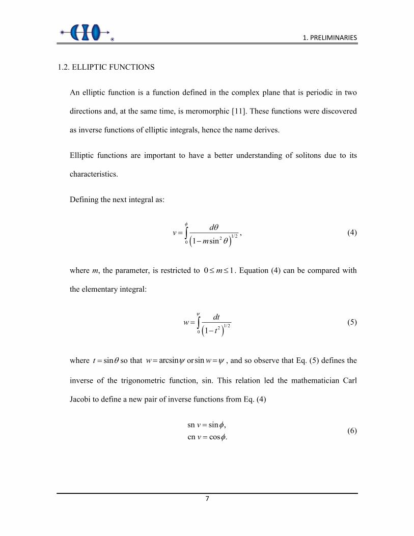
1.2. ELLIPTIC FUNCTIONS

An elliptic function is a function defined in the complex plane that is periodic in two

directions and, at the same time, is meromorphic [11]. These functions were discovered

as inverse functions of elliptic integrals, hence the name derives.

Elliptic functions are important to have a better understanding of solitons due to its

characteristics.

Defining the next integral as:

1/220

,1 sin

dvm

(4)

where m, the parameter, is restricted to 0 1m . Equation (4) can be compared with

the elementary integral:

1/220 1

dtwt

(5)

where sint so that arcsinw orsin w , and so observe that Eq. (5) defines the

inverse of the trigonometric function, sin. This relation led the mathematician Carl

Jacobi to define a new pair of inverse functions from Eq. (4)

sn sin ,cn cos .

vv

(6)

1. PRELIMINARIES

8

These are two of the twelve Jacobian elliptic functions (those functions can be

constructed with the aid of the Argand diagram shown in Fig. 4) and are normally

written as sn(v|m) and cn(v|m). To denote the parameter dependence (it is usual also to

work with the modulus, k, where 2m k [12].

The two special cases for 0,1m enable Eqs. (4) and (6) to be reduced to elementary

functions: if m = 0 then, v = ϕ and so cn(v|0) = cos ϕ = cos v, and if m = 1 the integral

can be evaluated to yield arcsech cosv and so cn(v|1) = sech v. It therefore follows

that cn(v|m) and sn(v|m) are periodic functions for 0 1m , but that periodicity is lost

for m = 1. Now the period of cn and sn corresponds to the period 2π of cos and sin, and

so the period of these elliptic functions can be written as:

2 /2

1/2 1/22 20 0

41 sin 1 sin

d d

m m

(7)

This latter integral is the complete elliptic integral of the first kind (because it’s

bounded),

/2

1/220

.1 sin

dK mm

(8)

It is obvious that K (0) = π/2, and it is also straightforward to show that K (m) increases

monotonically as m increases. In fact 1 log 16 / 12

K m m as 1m , and so

1. PRELIMINARIES

9

K m as 1m , this demonstrate the infinite period of the cn(v|1) = sech v

function.

FIGURE 4. Argand diagram constructed to show the formation of the Jacobi elliptic

functions

1.3. CNOIDAL WAVE

Another important contribution of Korteweg-de Vries was the cnoidal wave. The

cnoidal wave is an exact non-linear periodic solution to the KdV equation [5]. These

solutions are described in terms of the Jacobi elliptic function cn, hence their name

came from.

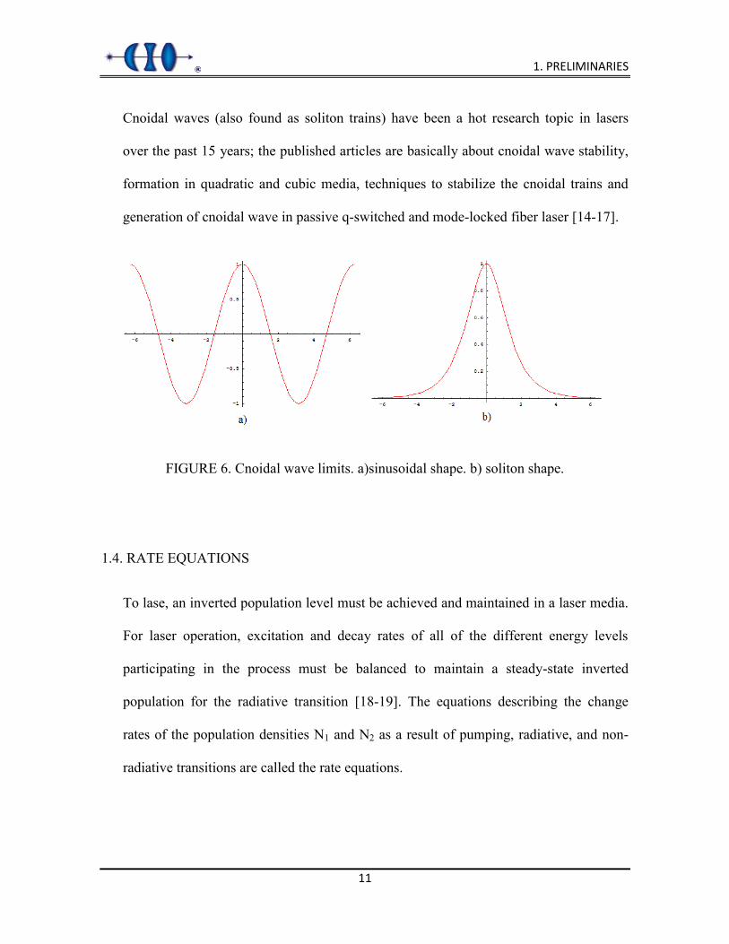
The main characteristic of these waves is that they are parametrically bounded by the

parameter (i.e. ellipticity); they change their shape from a sinusoidal (when the

ellipticity is zero) to a soliton-like (when the ellipticity tends to one) as shown in Fig. 5.

1. PRELIMINARIES

10

FIGURE 5. Cnoidal wave profile achieved for different parameter’s value.

These waves are not exclusive for the KdV equation; they can be found in any system

able to produce solitons (e.g. Boussinesq equations, non-linear Schrödinger equation,

shallow water equations, Sine-Gordon equation) [1-13].

The amplitude A(x,t) as a function of the horizontal position, x, and time, t, for a cnoidal

wave is given by:

22, cn 2 |x ctA x t A H K m m

(9)

where A2 is the trough elevation, H is the wave height, c is the phase speed and λ is the

wavelength. Further cn correspond to one of the Jacobi elliptic functions and K (m) is

the complete elliptic integral of the first kind; both depend on the elliptic parameter m.

This parameter determines the cnoidal wave shape; for m = 0 the cnoidal wave becomes

a cosine function, while for 1m the cnoidal wave is transformed into a hyperbolic

secant function, as is illustrated in Fig. 6.

1. PRELIMINARIES

11

Cnoidal waves (also found as soliton trains) have been a hot research topic in lasers

over the past 15 years; the published articles are basically about cnoidal wave stability,

formation in quadratic and cubic media, techniques to stabilize the cnoidal trains and

generation of cnoidal wave in passive q-switched and mode-locked fiber laser [14-17].

FIGURE 6. Cnoidal wave limits. a)sinusoidal shape. b) soliton shape.

1.4. RATE EQUATIONS

To lase, an inverted population level must be achieved and maintained in a laser media.

For laser operation, excitation and decay rates of all of the different energy levels

participating in the process must be balanced to maintain a steady-state inverted

population for the radiative transition [18-19]. The equations describing the change

rates of the population densities N1 and N2 as a result of pumping, radiative, and non-

radiative transitions are called the rate equations.

1. PRELIMINARIES

12

FIGURE 7. Two energy levels diagram including life-times

Consider the energy diagram of Fig. 7. Levels 1 and 2 have overall life-times τ1 and τ2,

respectively, permitting transitions to lower levels. The lifetime of level 2 has two

contributions: one associated with decay from 2 to 1 (τ21), and the other (τ20) associated

with decay from 2 to all other lower levels. When several modes of decay are possible,

the overall transition rate is a sum of the component transition rates. Since the rates are

inversely proportional to the decay times, the reciprocals of the decay times must be

added as 1 1 12 21 20 . Multiple modes of decay therefore shorten the overall life-time.

Aside from the radiative spontaneous emission component (with time constant sp ) in

21 , a non-radiative contribution, nr , may also be present, so that 1 1 121 sp nr .

If a system like the illustrated in Fig. 7 is allowed to reach the steady-state, the

population densities N1 and N2 will vanish by virtue of all the electrons ultimately

decaying to lower levels.

1. PRELIMINARIES

13

FIGURE 8. Energy levels 1 and 2 with surrounding higher and lower energy levels

Steady-state populations of levels 1 and 2 can be maintained, however, if energy levels

above level 2 are continuously excited and leak downward into level 2, as shown in the

more realistic energy level diagram of Fig. 8. Pumping can bring atoms from levels

other than 1 and 2 out of level 1 and into level 2, at rates R1 and R2 (per unit volume per

second), respectively. Consequently, levels 1 and 2 can achieve non-zero steady-state

populations.

1.4.1. RATE EQUATIONS IN THE ABSENSE OF AMPLIFIER RADIATION

The population densities increase rate of levels 2 and 1 arising from pumping and decay

are:

2 22

2

1 1 21

1 21

,

.

dN NRdt

dN N NRdt

(10)

1. PRELIMINARIES

14

Under steady-state condition ( 1 2 0N N ), Eqs. (10) can be solved for N1 and N2 and

the population difference N0 = N2 – N1 can be found. The result is:

10 2 2 1 1

21

1 .N R R

(11)

1.4.2. RATE EQUATIONS IN THE PRESENCE OF AMPLIFIER RADIATION

The presence of radiation near the resonance frequency enables transitions between

levels to take place by the processes of stimulated emission and absorption as well,

characterized by the probability density Wi and shown in Fig. 9. The Eqs. (10) must be

extended to include this source of population variation in each level

2 22 2 1

2

1 1 21 2 1

1 21

,

.

i i

i i

dN NR N W N Wdt

dN N NR N W N Wdt

(12)

Under steady-state condition ( 1 2 0N N ) eqs. (12) can be solved for N1 and N2, thus,

the population difference N = N2 – N1 is found.

0

22 1

21

with 1

1 ,

s i

s

NNW

(13)

where τs is the characteristic time which is always positive since 2 21 .

1. PRELIMINARIES

15

FIGURE 9. The population densities N1 and N2 (cm-3s-1) of atoms in energy levels 1 and 2

are determined by three processes: decay (b), pumping(r), and absorption and stimulated

emission (g)

1.5. STATZ – DE MARS MODEL

The rate equations proposed by H. Statz and G. de Mars (SdM) are independent of the

number of the laser’s energy levels because are based in the phenomenology that leads

the laser to emit stimulated radiation [20]. This characteristic allows to model different

types of laser systems (e.g. dye, solid state, semiconductor, fiber). This model is given

by the following set of equations:

( )' ( ) ( ) ,

( )' ( ) ( ) ,

dM M tB M t N tdt T

dN No N tB M t N tdt

(14)

where N(t) represents the population inversion density and M(t) the emitted photon

density at a determinate frequency. The emitted photon density is directly linked with

1. PRELIMINARIES

16

the photon-flux density S(t). If we divide the photon-flux between the propagation

speed of light v and the photons energy hv we obtain the emitted photons density; this

is:

( )( ) .S tM tvh

(15)

The constant B’ means ,Bh where B is the Einstein coefficient for stimulated

transitions. T represents the photons life-time inside the resonant cavity, which is

inversely proportional to the sum of the losses coefficients ξ1 and ξ2:

1 2

1Tv

(16)

τ represents the relaxation time of the population inversion difference between levels

where the laser emission takes place; β is a constant that depends of the level numbers

of the system and N0 stands for the equilibrium value of the population inversion

density achieved in absence of laser oscillation.

The physical interpretation of the SdM equations is especially simple. The first equation

states that the photons density grows as a consequence of the stimulated transitions

inside the cavity and decreases due to losses imputable to the medium and the resonator

[21]. The growth of the emitted photons density to a certain frequency is directly

proportional to the product of the same emitted photons quantity at that frequency by

the population inversion density of the laser medium. The second equation shows that

1. PRELIMINARIES

17

the population inversion density will decrease because of the stimulated emission and

will grow due to the pumping action on the upper energy levels of the medium.

1.6. SATURABLE ABSORBERS

A saturable absorber (SA) is a non-linear optical component with a certain optical loss,

which is reduced at high optical intensities [18]. SAs are usually used for passive mode-

locking and Q-switching depending on their parameters. It is well known that

continuous wave dye lasers with SAs provide short pulses due to self-stabilization of

the pulse shaping process. A SA inserted into a laser cavity increases the nonlinearity of

such system and enriches the laser operation dynamics. Mode-locking laser dynamics

has been an important study subject, traditionally mode-locking is actively obtained

with an optical modulator inside the cavity or passively with a SA.

The principal characteristics of a SA are: modulation depth (maximum possible change

in optical loss), unsaturable losses (unwanted losses which cannot be saturated),

recovery time, saturation fluence, saturation energy and damage threshold (given in

terms of intensity) [22].

When dealing with pulses, a fast saturable absorber has a recovery time well below the

pulse duration, while a slow absorber has it well above the pulse duration. The same

device may be either a fast absorber or a slow absorber, depending on the pulses used

with [19]. The saturation parameter of a saturable absorber is the ratio of the incident

pulse fluence to the saturation fluence of the device.

1. PRELIMINARIES

18

FIRST CHAPTER REFERENCES

1. P. G. Drazin and R. S. Johnson, Solitons: An introduction. 2nd ed. (Cambridge

University Press, 1989).

2. J. S. Russell, ―Report on waves‖, Fourteenth Meeting of the British Association for

the Advancement of Science (1844).

3. Lord Rayleigh, ―On waves‖, Phil. Mag. 1, 257-279 (1876).

4. J. de Boussinesq ―Théorie des ondes et des remous qui se propagent le long d'un

canal rectangulaire horizontal en communiquant au liquide continu dans ce canal

des vitesses sensiblement pareilles de la surface au fond‖, J. Math. Pures et

Appliquées 2, 55 (1872).

5. D. J. Korteweg and G. de Vries, "On the Change of Form of Long Waves

advancing in a Rectangular Canal and on a New Type of Long Stationary

Waves", Phil. Mag. 39, 422–443 (1895).

6. E. Fermi, J. Pasta, and S. Ulam, ―Studies of Nonlinear Problems‖, Document LA-

1940 (May 1955).

7. N. J. Zabusky and M. D. Kruskal, ―Interaction of 'Solitons' in a collisionless plasma

and the recurrence of initial states‖, Phys. Rev. Lett. 15, 240-243 (1965).

8. M. Wadati, ―Introduction to solitons‖, Pramana J. Phys. 57(5), 841-847 (2001).

9. N. Akhmediev and A. Ankiewicz, Solitons Nonlinear Pulses and Beams (Chapman

& Hall, 1997).

10. G. P. Agrawal, Optical solitons, autosolitons and similaritons. (Institute of Optics,

Rochester, NY, 2008).

1. PRELIMINARIES

19

11. N. I. Akhiezer, Elements of the Theory of Elliptic Functions, (AMS, Rhode Island,

1990).

12. M. Abramowitz and I. A. Stegun, Handbook of Mathematical Functions with

Formulas, Graphs, and Mathematical Tables, (New York: Dover, 1965).

13. D. Powell, ―Rogue waves captured‖, ScienceNews 179(13), 12 (2011).

14. C. Newell and J. V. Moloney, Nonlinear Optics (Addison-Wesley Publishing Co.,

1992).

15. Y. Yang, Solitons in field theory and nonlinear analysis. (Springer-Verlag, 2001).

16. N. Manton and P. Sutcliffe, Topological solitons (Cambridge University Press,

2004).

17. Y. A. Kartashov, A. A. Egorov, A. S. Zelenina, V. A. Vysloukh and L. Torner,

―Stabilization of one-dimensional periodic waves by saturation of the nonlinear

response‖, Phys. Rev. E 68, 065605(R) (2003).

18. A. E. Siegman, Lasers, (University Science Books, 1986).

19. O. Svelto, Principles of Lasers, Fourth edition, (Springer, 1989).

20. H. Statz and G. De Mars, ―Transients and Oscillation Pulses in Masers‖, Quantum

Electronics, 530-537 (1960).

21. L. Tarassov, Physique des Processus dans les Générateurs de Rayonnement

Optique Cohérent (Éditons MIR, 1981).

22. H. Haken, Laser Light Dynamics, (North Holland Physics Publishing, 1985).

2. THEORETICAL MODEL

20

CHAPTER 2

THEORETICAL MODEL

2.0. INTRODUCTION

In this chapter the system configuration is presented, the modeling will be made and the

stability analysis of the obtained model will be performed. The system dynamics will be

discussed in order to find the best regions to control the system.

2.1. LASER SCHEME

The proposed configuration is composed by a laser made up with an active medium

(AM), two mirrors (total reflexion, M1, and semitransparent, M2) and an intracavity

saturable absorber (SA) coupled with a low-power continuous wave laser (CW) through

an electro-optical modulator (EOM) as shown in Fig. (10)


21

FIGURE 10. Optical scheme for a laser system with an active saturable absorber. AM and

SA are active medium and saturable absorber, M1 and M2 are total reflected and semi-

transparent laser mirrors, and EOM is an electro-optical modulator.

2.2. LASER MODEL

Is assumed that the proposed system is a three-level laser [1] obeying the following

equations:

1 21 ( ) ( ) ( ) ( ),

( ) 2 ( ) ( ) 1 ,

dS t N t S t S tv dtdN t nS t N t Z

dt h

(17)

where: S(t) and N(t) stands for the photon-flux density and the population inversion

density inside the cavity, σ is the effective cross-section of interaction between active

centers and photons; the coefficient for absorption and dispersion is represented by ξ1


22

meanwhile the coefficient of the losses that depend on the mirrors reflectivity is ξ2; v is

the speed of light in the medium, τ represents the life-time between energy levels, n

stands for the number of active centers per volume unit on the medium and pZ W

where Wp represents the stimulated emission transition probability and finally is the

photon energy.

The saturable absorber will be modeled by two-level active resonant centers [2,3], so

that all the active absorbents centers are on a lower energy level to get the resonant

photons to cause the maximum opacity. The rate equations that describe the active

centers of the absorber are:

2 21 2

1 22 1

,

,

dn nS SB n B ndt v v

dn nS SB n B ndt v v

(18)

where Bα is the Einstein coefficient for stimulated emission on the absorber, and 1 / τα

is the probability of spontaneous emission for the absorbers active centers. Denoting by

n1α and n2α the density of active centers of the absorber in the lower and upper energy

levels, respectively, the total density of active centers of the absorber is given by

1 2n n n and then we have that in t = 0

1

2

,0.

n nn

(19)

When enough power-pump is applied the saturation condition can be achieved


23

1 2 .2nn n

(20)

Population inversion density of the absorber is defined as 2 1 ,N n n deducing

from Eqs. (19) and (20):

2 .N ndN B N S

dt v

(21)

Defining the absorption coefficient for the absorber as:

,k N (22)

where is the effective section of stimulated emission given by ,

vB

where

v represents the speed of light on the absorber and ω is the angular frequency.

If we multiply Eq. (21) by , it can be rewritten as:

02 ,v

k kdk B k Sdt

(23)

where 0k is the initial absorption coefficient given by 0 0k N n .

Steady-state implies that 0dkdt , and Eq. (23) becomes:

0 ,1

Sat

kk SS

(24)


24

where Sat

S is the photon-flux in where the absorption coefficient k falls down to half

its initial value 0k .

Being the non-resonant absorption coefficient, K the total absorption coefficient

of the absorber defined as: .K k Once this relation is satisfied, the photon flux

average equation of the active medium may be expressed by:

1( ) ,t

mS m m

d SLS L N S L Sv dt

(25)

where Lm is the active medium length.

The photon-flux average equation inside the absorber is given by:

(

t

m mS

m m l

d SL L L L LSv v c dt

L N S L N S L S L S

(26)

And the filling-coefficient of the cavity as:

/( )( )

m m

mm m m

L n L vL L LL n L n L L L L L

v v c

(27)

where /n c v and /n c v are the refractive index on the active medium and inside

the absorber, respectively, L is the cavity length and Lα the saturable absorber length.

Because 2( )( ),tS mS L S

Eq. (26) becomes then:


25

1 21 .v m m

L LdS N N S Sdt L L

(28)

This is the photon-flux equation inside a cavity with an active medium and a saturable

absorber, as shown in Fig. 11.

FIGURE 11. A laser cavity with an active medium and a saturable absorber.

Given that k N and defining T as the photons life-time inside a cavity with the

form 1

1 2 ,m

LTL

Eq. (23) can be rewritten as:

1 .m

LdS v NS v k S Sdt L T

(29)


26

Therefore, for a complete description of a laser with saturable absorber, only three

equations are needed: the photon-flux equation, an equation for the population inversion

density on the active medium and the saturable population inversion equation that gives

the saturation coefficient (taking into account k N ):

0

0

1 ,

,

2 .

m

LdS v NS v k S Sdt L T

N NdN NSdt hdk k S k kdt

(30)

In order to have an easier handling [4] of the Eqs. (30) the next non-dimensional

parameters are defined: t’ = t / τ, G = τ / T, δ = τ / τα, ρ = 2σα / βσ, α = ΓvσTN and αα = -

ΓvTk0αLα / Lm = - ΓvTσαnα / Lm; the new variables are: n(t’) = ΓvσTN(t’), nα(t’) = -

ΓvTkα(t’)Lα / Lm and m(t’) = βBτS(t’) / v = βστS(t’) / hω. With these new adimensional

parameters and variables, the Eqs. (30) can be rewritten as:

1 ,'

1 ,'

.'

dm Gm n ndtdn n mdtdn n mdt

(31)

All the parameters used to define the saturable absorber are fixed, except for αα, which

includes a measure of the active centers absorbent density, for this reason, αα will be

used as the saturable absorber’s identifying parameter.


27

The next step is to add an external modulation directly into the saturable absorber. The

best way to do this is through its main parameter (i.e. αα). Considering a CW low-

energy laser which output is normalized and an EOM which responds linearly to the

modulation injected energy (sinusoidal shape), Eqs. (31) are transformed into:

1 ,'

1 ,'

1 cos.

' 2c

dm Gm n ndtdn n mdt

tdn n mdt

(32)

where ωc stands for the modulation frequency applied to the EOM.

These three differential equations represent the working system, it must be noted that,

in absence of modulation frequency applied to the EOM, ω, the system returns to Eqs.

(31), i.e. rate equations for a laser with a passive saturable absorber.

2.3. LINEAR STABILITY ANALYSIS

Linear stability analysis (LSA) is used to understand the system dynamics [5]. The

analysis is based on the linear disturbance equations, these equations are derived from

the original equations. The method consists in linearizing the equations, obtain the

initial state condition (i.e. when the derivatives are zero), expand the system about the

initial state condition, construct the Jacobian matrix and find the eigenvectors and

eigenvalues with the determinant equal to zero [6]. This gives as a result the fixed


28

points of the equations system, which must be analyzed in order to know what type of

points are (i.e. fixed, source, saddle, etc.).

The equations of interest are Eqs. (32), these equations are non-autonomous due to the

explicit time-dependence found in the cosine of the third equation. To be able to

perform the LSA that dependence must be eliminated, to do that, a variable change

must be applied, giving as a result, the next equations system:

1 ,'

1 ,'

1 cos,

' 2

.c

dm Gm n ndtdn n mdt

xdn n mdtdxdt

(33)

Naming the Eqs. (33) as:

, , , 1 ,'

, , , 1 ,'

1 cos, , , ,

' 2

, , , .c

dmf m n n x Gm n ndtdng m n n x n mdt

xdnh m n n x n mdtdxj m n n xdt

(34)

Supposing that * * * *, , ,m n n x is the steady state, that is * * * *, , , 0,f m n n x

* * * *, , , 0,g m n n x * * * *, , , 0g m n n x and * * * *, , , 0.j m n n x


29

In order to know if the steady state is stable or unstable, a small perturbation

(represented by the subscript “p”) must be added to it

*

*

*

*

,

,

,

.

p

p

p

p

f f f

g g g

h h h

j j j

(35)

with , , , 1p p p pf g h j .

Now, the main question is: will the perturbations grow (steady state unstable) or decay

(steady state stable)?

To be able to observe if the perturbations grow or decay, the perturbations derivatives

must be found.

* * * *

* * * * * * * * * * * *

* * * * * * * *

( , , , ) ( , , , )

( , , , ) ( , , , ) ( , , , )

( , , , ) ( , , , ) high order terms

pp p p p

p p

p p

df dm f m n n x f m f n g n h x jdt dt

f m n n x f m n n x f f m n n x gm n

f m n n x h f m n n x jn x

(36)

Following the Taylor series expansion shown in Eqs. (36) the derivatives for each

perturbation are:


30

. . . . ,

. . . . ,

. . . . ,

. . . . ,

pp p p p

pp p p p

pp p p p

pp p p p

dff f f g f h f j

dt m n n xdg

g f g g g h g jdt m n n x

dhh f h g h h h j

dt m n n xdj

j f j g j h j jdt m n n x

(37)

The system presented in Eqs. (37) can be rewritten in the matrix form:

''

,''

p p p

p p p

p p p

p p p

f f f fm n n x

f f fg g g g

g g gm n n xh h h

h h h jm n n xj j j

j j j hm n n x

(38)

where denotes the Jacobian matrix of the original system at the steady state.

Substituting the values in the Jacobian function and the next matrix is obtained:

1 01 0 0

.0 sin( )

20 0 0 0

G n n Gm Gmn m

n m x

(39)


31

The next step is to find the eigenvectors and eigenvalues of the system 0,pI

so the determinant would be:

0.I (40)

The matrix for the former equation is:

1 01 0 0

0,0 sin( )

20 0 0

G n n Gm Gmn m

n m x

(41)

The solutions for the perturbed steady-state of the original system are:

0,,

,

0.

s

s

s

s

mnnx

(42)

Substituting the former solutions in Eqs. (41), the matrix transforms into:

1 0 0 01 0 0

0,0 0

0 0 0

G

(43)

Matrix (43) has the next characteristic equation:

1 1 0,G (44)


32

where 1 ( 1),G 2 1, 3 and 4 0 are eigenvalues which are all

real; being λ2 and λ3 always negative (i.e. the perturbation will decay) and λ4 is critically

stable. Therefore, the stability condition is defined only by the sign of λ1, i.e. the fixed

point is a source when 1 as shown in Fig. 12.

FIGURE 12. Stability condition given by the relation between α and αα.

SECOND CHAPTER REFERENCES

1. H. Statz, and G. De Mars, "Transients and Oscillation Pulses in Masers".

Quantum Electronics, 530-537 (1960).

2. L. Tarassov, Physique des processus dans les générateurs de rayonnement

optique cohérent (Éditons MIR, 1981).


33

3. C.L. Tang, H. Statz and G. de Mars, “Spectral output and spiking behavior of

solid-state lasers”, J. Appl. Phys. 34, 2289-2295 (1963).

4. M. Braun, Differential equations and their applications: An introduction to

applied mathematics (Springer, 1992).

5. L. C. Haber, Investigation of dynamics in turbulent swirling flows aided by

linear stability analysis, Ph. D. Thesis (Virginia Polytechnic Institute, 2003)

6. R. S. Palais, An introduction to wave equations and solitons (Chinese Academy

of Sciences, 2000).

7. L. W. Hilman, Dye laser principles (Academic press, 1990).

8. R. Paschotta, Encyclopedia of laser physics and technology (Wiley, 2008).

9. A. C. Newell and J. V. Moloney, Nonlinear Optics (Addison-Wesley Publishing

Co., 1992).

10. E. Infeld and R. Rowlands, Nonlinear Waves, Solitons and Chaos (Cambridge

University Press, Cambridge, 1990).

11. V. Aboites, K. J. Baldwin, G. J. Crofts, and M. J. Damzen, “Dye High Power

optical Switch”, Rev. Mex. Fis. 39 (4), 581 (1993).

12. C. E. Preda, B. Ségard, and P. Glorieux, “Comparison of laser models via laser

dynamics: The example of the Nd3+:YVO4 laser”, Opt. Commun. 261(1), 141-

148 (2006).

3. RESULTS AND CONCLUSIONS

34

CHAPTER 3

RESULTS AND CONCLUSIONS

3.0. INTRODUCTION

In this chapter the representing equations for the proposed experiment are numerically

solved in order to study the system dynamics. In some explored regions the cnoidal

waves are observed, the numerics were performed for different control parameters.

3.1. CONTROLLING THE SYSTEM DYNAMICS

To find the solutions of the Eqs. (32) a program was build using the typical Statz – de

Mars parameters for a Dye laser [1,2] G = 200, α = 4, δ = 1 and ρ = 0.001 and using as

initial condition a neighboring point to a system’s stable fixed point [3], i.e. m0 = 0.25,

n0 = 0 and nα0 = 0.152, that corresponds to a non-stationary fixed point neighboring.

As expected, when the modulation is not applied to the SA, the system tends to a fixed

point in a small computational time, as shown in Fig. 13. Once the modulation is

applied, the system starts to change into a periodic one as can be observed in Fig. 14.


35

FIGURE 13. Laser output without external modulation, the system tends to a fixed

point.

With a fixed modulation, the only parameter we can manipulate is αα, a measure of the

active centers absorbent density contained in the SA. Since all the geometrical values

involved in the definition of αα are fixed, the parameter αα will be identified as an

absorption ratio and therefore will depend on the chosen SA (in a dye SA its

dependence vary according to the dye concentration). For this numerical experiment, its

value was chosen in a practical range (between 0.3 and 60).

If all the physical parameters involved in this experiment are fixed, the available

variables are only the external modulation, represented by ωc, and the absorption ratio,

represented by αα. Due to this reason, the experiment is segmented in two parts. The

first one is realized with a fixed modulation frequency and varying absorption ratio, and

the second one is the reverse case, i.e. with fixed absorption ratio and varying

modulation frequency.


36

FIGURE 14. Laser output with fixed modulation (ωc = 1) and variable absorption ratio.

a) αα = 0.3, b) αα = 1, c) αα = 3, d) αα = 15, e) αα = 30 and f) αα = 60.

For the first case, when the Eqs. (32) were solved without modulation, the output

photon-flux, m, reached a fixed point in few iterations no matter the absorption ratio

used (transients), Fig. 13, as soon as the modulation is injected into the SA a periodic

train begins to appear with αα as small as 0.3, Fig. 14(a), as αα is increased the

maximum intensity reached increases and a region of different frequencies coexistence


37

(undamped undulations) begins to appear at a certain location in the pulse, the

localization of this region depends on the absorption ratio.

It can be observed from Fig. 13 that the laser output tends to a fixed point when the SA

is in passive configuration, i.e. without external modulation; as soon as the SA is turned

into an active device (Fig. 14), different packages of pulses are obtained depending on

the SA’s absorption ratio (αα), the bigger the concentration the higher the reached

intensity. The laser output, in this case, goes from a continuous wave regime to a high-

intensity peaks train passing, through an undamped undulations window moving across

the pulse’s body.

When the absorption ratio is larger than a threshold that depends on the modulation

frequency, the phase diagram between m and na exhibits instead of one, two critical

points, as shown in figure 15. When the frequency is normalized with the laser’s

relaxation frequency this phenomenon appears for an αa value near 1.4. If αa = 30 the

two critical points are separated in the phase space diagrams (figure 15(b)).

Being in the fixed point without modulation, the laser represents periodic oscillations

when the external modulation is applied and undergoes the period-doubling bifurcation

when the modulation frequency is increased.


38

FIGURE 15. Phase diagram m vs na. a) with αa = 1.4 b)with αa = 30.

For the second case (i.e. fixed absorption ratio), a comprehensive study on the output

signal in terms of ωc was done for an αa = 15, the value was chosen first of all because

the undamped undulations are obvious for small ωc and are nowhere near the maximum

intensity reached by the laser output; its behavior is representative of what happens at

any frequency even if there are some differences in detail.

Figure 16 shows how the signal frequency increases following the change in the

modulation frequency. As the frequency rises, a threshold is obtained where the narrow

pulse train is reached, its value is closely related with αa, a change in the absorption

ratio only moves the undamped undulations window; the window is shifted towards the

right (both thresholds get larger) as αa is increased. The second threshold corresponds to

the appearance of a narrow pulse train, when αa = 15 the narrow high intensity pulse

train is obtained at around ωc = 35.


39

FIGURE 16. Pulse shape at αa = 15 with different frequencies a) ωc = 1/4, b) ωc = 1/2,

c) ωc = 2, d) ωc = 5, e) ωc = 10, f) ωc = 35.

The dependence between the output pulse width and the modulation frequency, shown

in Fig. 17, is clearly a very good approximation to an exponential decay. It must be

noted that the modulation frequency ωc enters the equation as an integer multiple of the

laser relaxation frequency ω, so that the pulse duration is calculated from the relaxation

time. From the above considerations one can observe a width lower limit around 19 ns

achieved approximately at 80 KHz, which is 35 times the relaxation frequency.


40

FIGURE 17. Pulse width against control frequency. It is shown how the pulses width

become narrower as the control frequency is increased.

3.2. CNOIDAL WAVE OBSERVATION

Figure 18 shows the temporal dynamics of the laser output for fixed αa = 15 and

different modulation frequencies ωc. For small ωc (lower than the laser relaxation

oscillation frequency), the laser generates pulse trains with localized undulation

windows, which are the damped relaxation oscillations (Figs. 18(a)--18(c)). For higher

ωc, only one frequency remains, i.e. the laser oscillates with the modulation frequency

(Figs. 18(d)--18(f)), and the pulse shape strongly depends on ωc. One important aspect

is that as ωc is increased; the peak amplitude first increases, reaches a maximum, and

then decreases, thus going from a sech2 (when the amplitude is maximum, Fig. 18(d)) to

almost harmonic oscillations (Fig. 18(f)). While the peak amplitude is decreasing, the

laser intensity never falls down to zero again; the continuous background appears


41

because the frequency applied to the SA is so high that it has not enough time, neither

to relax to its ground state nor to saturate. As ωc further increases, the signal behavior

becomes more and more sinusoidal with relatively small amplitude. We repeat the

simulations for different αa with a step of 5 and find that the results shown in Fig. 18 for

αa = 15 follow exactly the same qualitative pattern for any other αa [5, 60].

In 2004, Y. Kartashov et al [4,5] demonstrated that certain cnoidal waves can be forced

to stabilized (this because normally the cnoidal waves are unstable), that forced-stable

waves were bounded, as in this case, by two values of control parameter; in the case

presented here, the boundaries are given by the modulation frequency.

It must be noted that the cnoidal waves obtained through the presented scheme are

founded in the inverse expected order, first, the upper limit was achieved (the soliton

shape) and, second the sinusoidal shape (the cosine limit).

The obtained pulse trains are asymptotically stable due to the quadratic non-linearities

given by the SA.


42

FIGURE 18. Laser output intensity for αa = 15 and control frequencies (a) ωc = 1, (b) 5,

(c) 15, (d) 25, (e) 50, and (f) 75.

Another interesting feature of the observed dynamics is that when the pulse train

amplitude reaches its maximum, a sech2 (soliton-like) shape approximates the pulse

shape with a very good precision as demonstrated in Fig. 19. This is confirmed by

overlapping one pulse with a sech2 waveform; the difference that appears on the base

right hand side is very small (in the order of 2%, and always less than 5%). We find that

for every saturable absorber coefficient αa there is an optimal modulation frequency ωs


43

for which this soliton-shape approximation has better precision than for other

frequencies.

As seen from Fig. 20, ωs increases approximately linearly with αa with two jumps at αa

= 5 and αa = 30. We should note that several theoretical and experimental works report

the existence of solitons meaning that the pulses shape obtained at the output presents

the soliton characteristic functions (sech and sech2). While in the cited works, the

difference between the reported pulses and the soliton shape is larger than 5%; our

system allows the soliton generation with a higher precision, which makes it prominent

for optical communication purposes.

FIGURE 19. Overlapping of one pulse taken at αa = 15 and ωc = 25 (solid line) with a

sech2 wave form (dashed line).


44

FIGURE 20. Modulation frequency ωs and absorption ratio of saturable absorber

corresponding to soliton-shape pulses.

3.3. CONCLUSIONS

This work effectively shows how a saturable absorber can be made in to an active

device to control the output of a laser.

The insertion of a modulated signal directly into the saturable absorber modifies the

continuous output driving it into a periodic one. The larger the αa the higher the laser

intensity obtained, and the more comb-like it becomes. For a given αa there are two

important thresholds: the modulation frequency where the undamped undulations

appear and the one where they disappear, as the absorption ratio is increased, the

undulations window is shifted towards higher frequencies.

For a given αa, as the modulation frequency is increased, the output signal changes from

a smooth periodic function to a clear comb-like pulse train whose width decreases

exponentially, thus the saturable absorber is behaving as an active device.


45

It was also demonstrated with a rate equations model (based on SdM) that a laser with

an active saturable absorber under the influence of a control radiation from another

laser can generate cnoidal waves within a certain range of control parameters, which

bound soliton-like and sinusoidal regimes.

No matter the physical saturable absorber characteristics, there is always a certain value

of the modulation frequency that would result in the cnoidal waves generation.

When we compared the resulting pulses with a typical soliton shape (sech2), we

obtained less than 5% error at the pulse base. The proposed system can be a base for

building a reliable and cheap device to generate cnoidal waves as efficient information

carriers for optical communication; the proposed system is economic due to the

elements involved, at using general purpose laser elements and not ultra-fast optics

elements, the experimental implementation of the presented scheme results less

expensive.

3.4. FUTURE WORK

In this thesis the studies were done with a simple rate-equations model, we believe that

the obtained results can be applied to different laser systems (e.g. Erbium-doped fiber

laser) and not only to Dye lasers.

As part of the future work, a more complete model will be studied theoretically and

experimentally.

The following experiment was implemented as a preliminary experimental attempt:

A 1550-nm EDFL diode pumped at 980-nm was used; the experimental array is shown

in Fig. 21. A 4-m Fabry-Perot laser cavity was formed by an active heavily doped 90-


46

cm-long erbium fiber, a Faraday rotating mirror (FRM) and a fiber Bragg grating (FBG)

with a 100-pm FWHM bandwidth, having, respectively, 100% and 98% reflectivities.

FRM was used in order to avoid polarization mode beating. An electro-optical

modulator (EOM), modulated through a functions generator, was placed inside the

cavity. The fiber output, after passing through a wavelength-division multiplexer

(WDM) was recorded with a photodetector and analyzed with an oscilloscope. The

pump-diode current was fixed at 64 mA, which results in a pump power of 15.5 mW.

This corresponds to about 10% over the laser threshold of 14 mW. This value was

chosen in order to obtain CW laser operation. The EDFL’s relaxation frequency is

around 28 kHz due to the applied pump power.

FIGURE 21. Experimental set-up implemented for search cnoidal waves.

Figure 22 shows preliminary results obtained for the shown configuration, these pulses

are generated when the frequency applied to the EOM is around 9.1 MHz, which

correspond to 325 times the laser’s relaxation frequency. It is expected that if the


47

erbium-doped fiber length changes, the frequency needed to generate cnoidal waves

would be shifted, if the length is reduced, so the frequency would be diminished and

conversely.

FIGURE 22. Experimental cnoidal wave limits. a) soliton-shape limit, b) sinusoidal shape

limit.

It is important to complete the experimental part of this work in order to be able to

construct a cheap cnoidal wave generator that can be reliable used with optical

communications purposes.

THIRD CHAPTER REFERENCES

1. M. J. Damzen, K. J. Baldwin, and P. J. Soan, “Optical switching and high-

resolution image transfer in a saturable dye spatial light modulator” J. Opt. Soc.

Am. B 11, 313 - 319 (1994).

2. L. W. Hilman, Dye laser principles (Academic press, 1990).


48

3. V. Aboites, K. J. Baldwin, G. J. Crofts, and M. J. Damzen, “Fast high power

optical switch”, Opt. Comm. 98, 298 - 302 (1993).


“Stabilization of one-dimensional periodic waves by saturation of the nonlinear

response”, Phys. Rev. E 68, 065605(R) (2003).


“Stable multicolor periodic-wave arrays”, Phys. Rev. Lett. 92(3) (2004).

6. P. G. Drazin and R. S. Johnson, Solitons: An introduction. 2nd ed. (Cambridge

University Press, 1989).

7. N. Akhmediev and A. Ankiewicz, Solitons Nonlinear Pulses and Beams

(Chapman & Hall, 1997).

8. L. Tarassov, Physique des Processus dans les Générateurs de Rayonnement

Optique Cohérent (Éditons MIR, 1981).

9. P. P. Sorokin and J. R. Lankard, “Stimulated emission observed from an organic

dye chloro-aluminum phthalocyanine” IBM J. Res. Develop. 10, 162-3 (1966).

10. B. K. Garside and T. K. Lim, “Laser mode locking using saturable absorbers”, J.

Appl. Phys. 44 (5), 2335 (1973).

11. W. Dietel, E.Döpel and D. Kühlke, “Passive mode locking of an argon laser

using rhodamine 6G saturable absorber and double mode locking of the pump

and dye laser system”, Sov. J. Quantum Electron. 12, 668 (1982)


49

12. V. V. Nevdakh, O. L. Gaiko, L. N. Orlov, “New operation regimes of a CO2

laser with intracavity saturable absorber”, Opt. Comm. 127, 303 - 306 (1996).

13. A. N. Pisarchik, A. V. Kir'yanov, Y. O. Barmenkov, and R. Jaimes-Reátegui,

"Dynamics of an erbium-doped fiber laser with pump modulation: theory and

experiment," J. Opt. Soc. Am. B 22, 2107-2114 (2005).

14. M. E. Fermann, “Passive mode locking by using nonlinear polarization

evolution in a polarization-maintaining erbium-doped fiber”, Opt. Lett. 18 (11),

894 (1993).

15. Schmidt et al., “Passive mode locking of Yb:KLuW using a single-walled

carbon nanotube saturable absorber”, Opt. Lett. 33 (7), 729 (2008).

16. W. Dietel et al., “Passive mode locking of an argon laser using rhodamine 6G

saturable absorber and double mode locking of the pump and dye laser system”

Sov. J. Quantum Electron, 12 (5), 668 (1982).

17. N. J. Zabusky and M. D. Kruskal, “Interaction of 'Solitons' in a collisionless

plasma and the recurrence of initial states”, Phys. Rev. Lett. 15, 240-243 (1965).

18. J. E. Bjorkholm and A. A. Ashkin, “Cw self-focusing and self-trapping of light

in sodium vapor”, Phys. Rev. Lett. 32, 129-132 (1974).

19. F. Gèrôme, P. Dupriez, J. Clowes, J. C. Knight and W. J. Wadsworth, “High

power tunable femtosecond soliton source using hollow-core photonic bandgap

fiber, and its use for frequency doubling”, Opt. Express 16, 2381-2386 (2008).


50

20. R. Herda and O. G. Okhotnikov, “All-fiber soliton source tunable over 500 nm”,

in Conference on Lasers and Electro-Optics/Quantum Electronics and Laser

Science and Photonic Applications Systems Technologies, Technical Digest

(CD) (Optical Society of America, 2005), paper JWB39.

21. S. Chouli and P. Grelu, “Rains of solitons in a fiber laser”, Opt. Express 17,

11776-11781 (2009).

22. J. Li, X. Liang, J. He, L. Zheng, Z. Zhao and J. Xu, “Diode pumped passively

mode-locked Yb:SSO laser with 2.3ps duration”, Opt. Express 18, 18354-18359

(2010).

23. M. G. Clerc, S. Coulibaly, N. Mujica, R. Navarro and T. Sauma, “Soliton pair

interaction law in parametrically driven Newtonian fluid”, Phil. Trans. R. Soc. A

367, 3213-3226 (2009).

24. J. M. Saucedo-Solorio, A. N. Pisarchik, A. V. Kir’yanov, and V. Aboites, “Generalized

multistability in a fiber laser with modulated losses,” J. Opt. Soc. Am. B 20, 490-496

(2003).

25. A. N. Pisarchik, Y. O. Barmenkov, and A. V. Kir’yanov, “Experimental

characterization of the bifurcation structure in an erbium-doped fiber laser with pump

modulation,” IEEE J. Quantum Electron. 39, 1567-1571 (2003).

26. L. H. Zao, and C. Q. Dai, “Self-similar cnoidal and solitary wave solutions of the

(1+1)-dimensional generalized nonlinear Schrödinger equation,” Eur. Phys. J. D 58,

327-332 (2010).


51

27. V. M. Petnikova, V. V. Shuvalov and V. A. Vysloukh, “Multicomponent

photorefractive cnoidal waves: Stability, localization, and soliton asymptotics,” Phys.

Rev. E. 60, 1009-1018 (1999).

28. A. N. Pisarchik, A. V. Kir’yanov, Y. O. Barmenkov, and R. Jaimes-Reátegui,

“Dynamics of an erbium-doped fiber laser with pump modulation: theory and

experiment,” J. Opt. Soc. Am. B 22, 2107-2114 (2005).

A1: LIST OF PUBLICATIONS

i

APPENDIX A

LIST OF PUBLICATIONS

A1.1. PEER-REVIEWED INDEXED JOURNALS

1. V. aboites, and M. Wilson, “Tinkerbell chaos in a ring phase-conjugated resonator”,

Int. J. Pure Appl. Math. 54(3), 429-435 (2009).

2. M. Wilson, and M. Huicochea, “Duffing chaotic laser resonator”, Iraqui J. Appl.

Phys. 1(5), 236-240 (2009).

3. M. Wilson, and M. Huicochea, “Driving a ring resonator’s dynamics into chaos”,

Int. J. Pure Appl. Math. 60(3), 239-245 (2010).

4. M. Wilson, V. Aboites, A. N. Pisarchik, V. Pinto, and Y. O. Barmenkov,

“Controlling a laser output through an active saturable absorber”, Rev. Mex. Fis.

57(3), 250-254 (2011).

5. M. Wilson, V. Aboites, A. N. Pisarchik, V. Pinto, and M. Taki, “Generation of

cnoidal waves by a laser system with a controllable saturable absorber”, Opt.

Express 19(15), 14210-14216 (2011).

A1: LIST OF PUBLICATIONS

ii

A1.2. CONFERENCES

1. M. Wilson, and V. Aboites, “Stability and chaos in a laser with an intracavity

saturable absorber”, Fourth international conference of pure and applied

mathematics, Plovdiv, Bulgaria (2007).

2. M. Wilson, “Photonic crystal fibers: uses and applications”, Sixth national

symposium of electronics and electro-mechanics” Los Mochis, Mexico (2008).

3. M. Wilson, and V. Aboites, “Resonador laser caótico de Duffing” LII Physics

National Conference, Acapulco, Mexico (2009).

4. D. Dignowity, V. Aboites, M. Wilson, and M. Huicochea, “Control de la dinámica

especial de un resonador láser” LII Physics National Conference, Acapulco, Mexico

(2009).

5. M. Wilson, V. Aboites, and A. N. Pisarchik, “Sincronización de una red de láseres

logísticos” XXIII Optics Anual Meeting, Puebla, Mexico (2010).

6. M. Wilson, V. Aboites, and A. N. Pisarchik, “Solitons formation in a laser with an

active saturable absorber” Mexican Conference of Complexity Sciences, Mexico

City, Mexico (2010).

7. M. Wilson, and V. Aboites, “Synchronization in a Gaussian lasers network”

Mexican Conference of Complexity Sciences, Mexico City, Mexico (2010).

8. M. Wilson, and V. Aboites, “Optical resonators and dynamic maps” 22th

International Conference of Optics, Puebla, Mexico (2011).

Documents

CNOIDAL WAVE FORMATION IN A LASER SYSTEM WITH …biblioteca.cio.mx/tesis/15032.pdf · on horseback, and overtook it still rolling on at a rate of some eight or nine miles an hour