Embed Size (px)
Citation preview

sensors
Article
CNN-Based Classifier as an Offline Trigger for the CREDOExperiment
Marcin Piekarczyk 1,* , Olaf Bar 1 , Łukasz Bibrzycki 1 , Michał Niedzwiecki 2 , Krzysztof Rzecki 3 ,Sławomir Stuglik 4 , Thomas Andersen 5 , Nikolay M. Budnev 6 , David E. Alvarez-Castillo 4,7 ,Kévin Almeida Cheminant 4 , Dariusz Góra 4 , Alok C. Gupta 8 , Bohdan Hnatyk 9 , Piotr Homola 4 ,Robert Kaminski 4 , Marcin Kasztelan 10 , Marek Knap 11 , Péter Kovács 12 , Bartosz Łozowski 13 ,Justyna Miszczyk 4 , Alona Mozgova 9, Vahab Nazari 14, Maciej Pawlik 3, Matías Rosas 15,Oleksandr Sushchov 4 , Katarzyna Smelcerz 2 , Karel Smolek 16 , Jarosław Stasielak 4 , Tadeusz Wibig 17 ,Krzysztof W. Wozniak 4 and Jilberto Zamora-Saa 18
�����������������
Citation: Piekarczyk, M.; Bar, O.;
Bibrzycki, Ł.; Niedzwiecki, M.;
Rzecki, K.; Stuglik, S.; Andersen, T.;
Budnev, N.; Alvarez-Castillo, D.;
Almeida Cheminant, K.; et al.
CNN-Based Classifier as an Offline
Trigger for the CREDO Experiment.
Sensors 2021, 21, 4804. https://
doi.org/10.3390/s21144804
Academic Editors: Ali Khenchaf
Received: 4 May 2021
Accepted: 8 July 2021
Published: 14 July 2021
Publisher’s Note: MDPI stays neutral
with regard to jurisdictional claims in
published maps and institutional affil-
iations.
Copyright: © 2021 by the authors.
Licensee MDPI, Basel, Switzerland.
This article is an open access article
distributed under the terms and
conditions of the Creative Commons
Attribution (CC BY) license (https://
creativecommons.org/licenses/by/
4.0/).
1 Institute of Computer Science, Pedagogical University of Krakow, 30-084 Kraków, Poland;[email protected] (O.B.); [email protected] (Ł.B.)
2 Faculty of Computer Science and Telecommunications, Cracow University of Technology,31-155 Kraków, Poland; [email protected] (M.N.); [email protected] (K.S.)
3 Department of Biocybernetics and Biomedical Engineering, AGH University of Science and Technology,30-059 Kraków, Poland; [email protected] (K.R.); [email protected] (M.P.)
4 Institute of Nuclear Physics, Polish Academy of Sciences, 31-342 Kraków, Poland;[email protected] (S.S.); [email protected] (D.E.A.-C.);[email protected] (K.A.C.); [email protected] (D.G.); [email protected] (P.H.);[email protected] (R.K.); [email protected] (J.M.); [email protected] (O.S.);[email protected] (J.S.); [email protected] (K.W.W.)
5 NSCIR, Thornbury, ON N0H2P0, Canada; [email protected] Applied Physics Institute, Irkutsk State University, 664003 Irkutsk, Russia; [email protected] Bogoliubov Laboratory of Theoretical Physics, JINR, 6 Joliot-Curie St, 141980 Dubna, Russia8 Aryabhatta Research Institute of Observational Sciences (ARIES), Manora Peak, Nainital 263001, India;
[email protected] Astronomical Observatory, Taras Shevchenko National University of Kyiv, UA-01033 Kyiv, Ukraine;
[email protected] (B.H.); [email protected] (A.M.)10 Astrophysics Division, National Centre for Nuclear Research, 28 Pułku Strzelców Kaniowskich 69,
90-558 Łódz, Poland; [email protected] Astroparticle Physics Amateur, 58-170 Dobromierz, Poland; [email protected] Institute for Particle and Nuclear Physics, Wigner Research Centre for Physics, Konkoly-Thege Miklós út
29-33, 1121 Budapest, Hungary; [email protected] Faculty of Natural Sciences, University of Silesia in Katowice, Bankowa 9, 40-007 Katowice, Poland;
[email protected] Joint Institute for Nuclear Research, Joliot-Curie Street 6, 141980 Dubna, Russia; [email protected] Institute of Secondary Education, Highschool No. 65, 12000 Montevideo, Uruguay;
[email protected] Institute of Experimental and Applied Physics, Czech Technical University in Prague, Husova 240/5,
110 00 Prague, Czech Republic; [email protected] Faculty of Physics and Applied Informatics, University of Lodz, 90-236 Łódz, Poland; [email protected] Departamento de Ciencias Fisicas, Universidad Andres Bello, Santiago 8370251, Chile;
[email protected]* Correspondence: [email protected]
Abstract: Gamification is known to enhance users’ participation in education and research projectsthat follow the citizen science paradigm. The Cosmic Ray Extremely Distributed Observatory(CREDO) experiment is designed for the large-scale study of various radiation forms that contin-uously reach the Earth from space, collectively known as cosmic rays. The CREDO Detector apprelies on a network of involved users and is now working worldwide across phones and other CMOSsensor-equipped devices. To broaden the user base and activate current users, CREDO extensivelyuses the gamification solutions like the periodical Particle Hunters Competition. However, theadverse effect of gamification is that the number of artefacts, i.e., signals unrelated to cosmic raydetection or openly related to cheating, substantially increases. To tag the artefacts appearing in the
Sensors 2021, 21, 4804. https://doi.org/10.3390/s21144804 https://www.mdpi.com/journal/sensors

Sensors 2021, 21, 4804 2 of 24
CREDO database we propose the method based on machine learning. The approach involves trainingthe Convolutional Neural Network (CNN) to recognise the morphological difference between signalsand artefacts. As a result we obtain the CNN-based trigger which is able to mimic the signal vs.artefact assignments of human annotators as closely as possible. To enhance the method, the inputimage signal is adaptively thresholded and then transformed using Daubechies wavelets. In thisexploratory study, we use wavelet transforms to amplify distinctive image features. As a result,we obtain a very good recognition ratio of almost 99% for both signal and artefacts. The proposedsolution allows eliminating the manual supervision of the competition process.
Keywords: image sensors; global sensor network; gamification; citizen science; convolutional neuralnetworks; image classification; deep learning; CREDO
1. Introduction1.1. CREDO Project
The Cosmic Ray Extremely Distributed Observatory (CREDO) is a global collaborationdedicated to observing and studying cosmic rays (CR) [1] according to the Citizen Scienceparadigm. This idea underpinned some other similar particle detection initiatives likeCRAYFIS [2–6] and DECO [7–10]. The CREDO project collects data from various CRdetectors scattered worldwide. Note that according to the project’s open access philosophy,the collected data are available to all parties who want to analyse them. Given the largeamount of potential hits registered in these experiments and the fact that only a fraction ofthem are attributable to particles of interest (mostly muons), effective on-line or off-linetriggers are a must. The on-line muon trigger described in [4] was based on the CNNwith a lazy application of convolutional operators. Such an approach was motivated bythe limited computational resources available in mobile devices. Here, we propose analternative approach to the CNN-based trigger design aimed principally at off-line use.However, the moderate size of convolutional layers in our design in principle allows foruse also with the limited resources of smartphones.
CR are high-energy particles (mostly protons and atomic nuclei) which move throughthe space [11]. They are emitted by the Sun or astrophysical objects like supernovae, super-massive black holes, quasars, etc. [12]. CR collide with atoms in the Earth’s atmospherethus producing secondary particles that can undergo further collisions, finally resulting inparticle air showers that near the Earth surface consist of various particles, mainly photonsand electrons/positrons but also muons. Muons are of principle interest to us because theirsignatures are easily distinguishable from other particles. Moreover, it is guaranteed thatthey are of cosmic origin as there are no terrestrial sources for muons. Such air showerscan be detected by various CR detectors. CR studies provide an alternative to studyinghigh-energy particle collisions in accelerators [13] and in terms of energies available surpassthem by several orders of magnitude. As the CR are ionising radiation, they can cause theDNA mutations [14], damage of hardware, data storage or transmission [15]. Monitoringthe intensity of the radiation flux (cosmic weather) is also important for manned spacemissions [16] and humans on Earth [17]. Existing detector systems are operating in isola-tion, whereas CR detectors used by the CREDO collaboration operate as part of a globalnetwork. This may provide new information on extensive air showers, or Cosmic RayEnsembles [1]. The CREDO project is gathering and integrating detection data provided byusers. The project is open to everybody who wants to contribute with their own detector.Most of the collected data comes from smartphones running the CREDO Detector app,operating on the Android system [18]. The physical process behind registering cosmic rayswith the app is identical to that used by silicon detectors in high-energy physics experi-ments. The ionising radiation interacts with the camera sensor and produces electron–holepairs [19]. Then, the algorithm in the app analyses the image from the camera and searchesfor CR hits. Signals qualified as hits of cosmic rays are then sent to the CREDO server.

Sensors 2021, 21, 4804 3 of 24
The overall scale of the CREDO observation infrastructure and the data collectedso far can be summarised in the following statistics (approximate values as of February2021): over 1.2× 10⁴ unique users, over 1.5× 10⁴ physical devices, over 1.0× 10⁷ candidatedetections registered in a database, and the total operation time of 3.9× 10⁵ days, i.e., morethan 1050 years.
1.2. Gamification as a Participation Driver
To arouse interest in cosmic ray detection with the CREDO Detector application amongprimary and secondary school pupils, university students and all interested astroparticleenthusiasts, an element of gamification was introduced. One of these elements is the“Particle Hunters” competition. In this competition, each participant teams up with otherparticipants under the supervision of a team coordinator who is usually a teacher fromtheir educational organisation. Each participating team’s goal is to capture as many goodcosmic ray particle candidates as possible using the above-mentioned CREDO Detectorapplication. The competition is played in two categories: League and Marathon.
• Competition in the League category: Consists of capturing particles during oneselected night of the month. During the competition, each month, on the night of the12th to the 13th of the month, competition participants launch the CREDO Detectorapplication between 9 pm and 7 am (local time of each team). The winner of thecompetition is chosen based on the number of particles captured during that onenight. In Figure 1, the day on which this event occurred (League) is indicated by adashed vertical green line.
• Competition in the Marathon category: Members of the team participating in thiscategory launch the CREDO Detector application at any time during the competition.At the end of the contest, the total number of detections made by all team membersfor the entire duration of the event is calculated, including detections made for theLeague category.
The competition lasts 9 months. The current third edition runs from 21 October 2020 to18 June 2021. The role of gamification in the CREDO project can be observed in a plot of thedaily activity of users of the CREDO Detector Application shown in Figure 1. A significantincrease in user activity during each edition of the “Particle Hunters” competition can beobserved.
Figure 1. Daily activity of the CREDO Detector application users from the premiere of the application (June 2018) to 1 March2021. Green lines show the days of the event in the competition for schools. Dashed black lines indicate the beginning andend of a given year. Horizontal red line reflects the average daily number of active users (97). Blue areas indicate areasbetween two editions of the competition (early July to early October).

Sensors 2021, 21, 4804 4 of 24
In particular, it can be seen that the daily activity of the CREDO application usershas changed since the competition inception. Statistically, about 97 users are active daily,but there is a decrease in the holiday season and an increased activity of users in periods ofcompetitions. There is also a visible decrease during the pandemic—where the possibilitiesof advertising the application (e.g., at science festivals) are very limited. The horizontalaxis shows the number of days from 1 January 2018. The application was launched (start)in June 2018.
The statistics of the last (completed) edition of the competition is shown in Table 1.The table compares results of all users with those participating in the competition.
Table 1. All participants vs. competition participants. Data collected from 1 October 2019 to30 January 2020).
All Competitors (% of All)
Users 1533 717 (47%)Teams 310 62 (21%)Devices 1756 836 (48%)Total time work [Hours] 459,000 170,000 (37%)Candidates of detections 1,207,000 812,000 (67%)Good Detections 558,000 242,000 (46%)% of good candidates 46% 30%
The above statistics show that during the competitions most of detections, i.e., 67%,come from the competitors. This proves the positive impact of the gamification uponthe CREDO project performance. Unfortunately, the data collection process is exposedto the cheating users, trying to deliver as many hits as possible. Significant part of dataare thus unusable for the research, because the percentage of good detection candidatesdecreases from 46% to 30%, see Table 1. Therefore, to be able to fully exploit the potentialof gamification, an efficient, fair, and intelligent detection filtering mechanism is required,and this is where machine learning capabilities come into play. More information aboutthe competition can be found on the official “Particle Hunters” website [20].
1.3. Data Management
The events being sent to the server can be corrupted. This is because the detectionfrom CCD/CMOS sensors is strongly dependent on the correct use. The Android appprovided by CREDO collaboration is working on the so-called dark frame, i.e., the imageregistered with the camera tightly covered. A user can, however, produce fake detections,by the corruption of the dark frame, e.g., with not fully covered sensor or use of an artificiallight sources to simulate cosmic ray hits. More obvious cases related to fakes and hardwaremalfunction can be relatively easy recognised and filtered. The simplest off-line filter thatis used in the competition is the anti-artefact filter, which consists of three parts of detectionanalysis [19]:
• Coordinate analysis—more than two events at the same location on two consecutiveframes are marked as hot pixels because they are statistically incompatible with themuon hit rate.
• Time analysis—hits are rejected if more than 10 detections are registered on a givendevice per minute, which is also incompatible with the expected muon hit rate.
• Brightness analysis—the frame cannot contain more than 70 pixels with luminancegreater than 70 in the greyscale.
Requirements defined above reduce the number of detections from 10.5 million toabout 4 million. More specifically, based on the time analysis, about 5.8 million hitswere rejected, while 380 thousand hits were rejected based on the brightness analysis,with another 0.8 million rejected based on the coordinate analysis.

Sensors 2021, 21, 4804 5 of 24
2. ANN-Based Method to Remove Artefacts
Analysis of data collected from various types of sensors is one of the most importantdriving forces in the development of computational intelligence methods. Significantchallenges are especially issues related to the multiplicity of sources (types of sensors),the operation of sensors in distributed systems, the exponential increase in the volume ofinformation received from them and very often the requirement to carry out the analysis inthe real-time regime. Tasks related to classification and recognition are often approachedby well-known statistical models [21,22], such as SVM [23], ANN [24] or RF [25]. Recently,deep learning models, based on various variants of neural networks, such as CNN [26],RNN [27] or GNN [28], are also experiencing a renaissance. Depending on the area andspecificity of applications, very complex approaches are used, often utilising integrationand combination of many techniques, which is particularly visible in case of interdis-ciplinary problems occurring, for example, in such selected fields as medicine [29,30],education [31,32], metrology [33–35], biometrics [36,37], learning of motor activities [38,39]or gesture recognition [40,41].
In image classification and recognition tasks, convolutional architectures (CNNs),regardless of depth, have a structural advantage over other types of statistical classifiersand usually outperform them. Therefore, in this paper, we chose to design an approachbased on deep convolutional networks. Several recognised CNN-based classifier modelswere considered, including AlexNet [42], ResNet-50 [43], Xception [44], DenseNet201 [45],VGG16 [46], NASNetLarge [46] and MobileNetV2 [47]. The possibilities of using theconcept of transfer learning were also analysed, where such networks are pretrained forlarge, standardised data sets, such as ImageNet [48]. The transfer learning approach toclassifying the CREDO data was already discussed in [49]. Due to the peculiarity of theproblem, quite unusual input data and a small spatial size of the signal in the images(only a few to a maximum of several dozen pixels), we decided to develop a dedicatedarchitecture tailored to the specifics and requirements of the problem. To obtain the optimalclassifier we explored different architectures (taking into account a constraint related tothe relatively low resolution of input images) and available hyperparameter values, likelearning rate, batch size, solver, regularisation parameters, pooling size, etc. Section 2.2presents the best classifier setup we found.
2.1. Experiment Design
The experiment was performed, and its flow chart is presented in Figure 2. The experi-ment consists of the following steps, where some of them are described in next subsectionsin detail:
• Data import. The source data are stored in the CREDO App database [18]. Data usedin this experiment were imported and stored in a more flexible format for furthercomputation.
• Data filtering. Due to a huge amount of useless data, including very typical andobvious artefacts, the robust and deterministic filtering algorithm with high specificitywas applied [50]. As a result, all non-artefact data are retained.
• Manual tagging. Manual tagging using web-based software [51] by five indepen-dent researchers was performed. As a result, four classes of images were obtained:535 spots, 393 tracks, 304 worms and 1122 artefacts. However, in this study we arefocused on a binary classification. Therefore, spots, tracks and worms made up oneclass (called collectively signal) and the artefacts the other. Given a manually labelleddataset, we can roughly estimate the annotators’ classification uncertainty in terms ofthe mean and standard deviation of the number of votes cast for an image that is asignal or artefact. Five people did a manual classification. We used samples whoseclassification was almost unanimous, i.e.,
– from 1232 signals 815 were classified by 5 of 5 and 417 were classified by 4 of 5,– from 1122 artefact are classified by 5 of 5.

Sensors 2021, 21, 4804 6 of 24
Therefore, an average signal vote can be calculated according the Equation (1):
(5× 815 + 4× 417)(815 + 417)
= 4.7 (1)
Respective probabilities of a given vote number for signal are
– 5/5 votes probability: 66%,– 4/5 votes probability: 34%,– standard deviation of votes: 0.48.
Thus, the overall vote number probability is 4.7± 0.5, which gives 10% of relativeuncertainty.
• Building a CNN model. The main part of the experiment is the Artificial NeuralNetwork model based on Convolutional Neural Network described in Section 2.2.
• Data preprocessing. We consider three approaches to preparing the input data: feedingraw data (Section 3.1), feeding wavelet transformed data (Section 3.2) and feeding thefusion of raw and wavelet transformed data (Section 3.3).
• Cross-validation. The model was trained and tested in a non-stratified repeated 5-foldcross-validation standard procedure, thus resulting in 25 classification results.
• Results evaluation. Finally, the results obtained were evaluated using accuracy calcu-lated as the fraction of correct classifications to overall classifications and are presentedin Section 3.
Data import
Import data fromCREDO App database
Data filtering
Filter data using pattern recognition robust algorithm
Manual tagging
Classes of images:● 1232 - signals● 1122 - artefacts
Data form selection
Building tailored CNN model
Results evaluation
Evaluation of the results based on the accuracy and confusion matrix analysis
Cross validation
Perform 5-fold cross validation including: split, fit and evaluation
Assigning data to classes:[spots, tracks, worms] collectively called signalsand artefacts.
Only raw dataOnly wavelet transformed
data
Combined raw and wavelet
transformed data
Figure 2. Computation experiment flow chart.
The computations were optimised with respect to various single wavelet transforma-tions performed during preprocessing.
2.2. CNN Model and Its Architecture
The Convolutional Neural Network (CNN) model shown in Figure 3 was build toperform the experiment. The model is moderately deep and its convolutional layers are

Sensors 2021, 21, 4804 7 of 24
moderately wide. The motivation for such an architecture was the potential to use it asthe lightweight trigger in the online applications. Therefore, the network we used had atypical architecture including convolutional, pooling and fully-connected layers. In thisarchitecture, the model hyperparameters to be configured include the size of filters andkernels, the activation function in convolutional layers, the size of the pool in poolinglayers, the output space dimensionality, the activation function and kernel initialiser aswell as their regularisers in fully-connected layers.
Figure 3. Layer-oriented signal flow in the convolutional network (CNN) artefact filtration model.
The best hyperparameter combination was found manually by performing manytrial and error cycles. Finally, we used the architecture that consisted of the layers and itsparameters which are listed in Table 2. The optimisation algorithm RMSProp [52] using abatch size of 64 was used as the solver. Additionally, for the fully-connected (dense) layers,a combined L1 and L2 regularisation (so-called Elastic Net [53]) with coefficients of 0.01was applied.
Table 2. Layer-by-layer summary of the proposed CNN model. Each layer name is given followedby the number of feature maps (convolutional layers) or neurons (dense layers), the size of theconvolutional filter or pooling region, the activation function used and, last, the number of parametersto learn.
Layer Type Features Size Activation Params
Convolution 2D 32 5 × 5 ReLU 832Max Pooling - 2 × 2 - -Convolution 2D 64 5 × 5 ReLU 51,264Max Pooling - 2 × 2 - -Convolution 2D 128 5 × 5 ReLU 204,928Max Pooling - 2 × 2 - -Convolution 2D 128 5 × 5 ReLU 409,728Max Pooling - 2 × 2 - -
Flatten 1152 - - -
Dense 300 - ReLU 345,900Dense 50 - ReLU 15,050
Dense 2 - Softmax 102
TOTAL PARAMS: 1,027,804TRAINABLE PARAMS: 1,027,804NON-TRAINABLE PARAMS: 0

Sensors 2021, 21, 4804 8 of 24
2.3. Applying Wavelet Transforms as Feature Carriers
The CNN input layer can be fed with raw images that in case of CREDO data are60 × 60 (RGB) three-layer colour images. Given the great diversity of artefact images interms of types and shapes we came up with a design which focuses on general imageproperties like the shape of the border or the connectedness of the image pattern. Thesegeneral properties can be amplified by applying wavelet transformation. As a result,one obtains the averaged image along with horizontal and vertical fluctuations whichamplify horizontal and vertical border components, respectively. Accordingly, the rawdata are subject to preprocessing as per the recipe below. The first preprocessing step isa greyscale conversion, which is implemented by summing up the channels. This step isaimed to remove a redundant information which does not carry any physical interpretation.The colour of the pixel is associated with the colour filter, overlaid on the CMOS array, thathappened to be hit during detection. This is basically a random event and is not correlatedto radiation species. The next step is the noise reduction. As the analysed images were ofdifferent overall brightness, we decided to apply a noise cut-off algorithm which dependson the average brightness. Moreover, images marked as “artefacts” usually differ from“non-artefacts” by a few standard deviations in brightness. The two above mentionedquantities were used to define the cut-off threshold, i.e., average and standard deviation ofbrightness (Equations (2) and (3)). The threshold was determined for each image separately.The standard deviation was calculated for the total brightness of each image:
ti = bi + 5σi (2)
where bi denotes mean of brightness and σi is a standard deviation of brightness of ith
image. Finally, the threshold used for noise reduction has the form
threshold =
{ti for ti < 100100 for ti ≥ 100
(3)
All pixels below the threshold are cut off. A set of images prepared in this way issubject to wavelet transform. More specifically, before feeding the images to the CNN, theDaubechies wavelet transformation was performed on them. Formally the original imagesignal f was transformed into four subimages according to the formula
f→
a | v− −h | d
, (4)
where subimage a denotes the average signal while h, v and d denote the horizontal,vertical and diagonal fluctuations, respectively [54]. All subimages have half the resolutionof the original image.
The full preprocessing flow for exemplary images selected from the dataset is pre-sented in Figures 4–7.
(a) Color (b) Grayscale (c) Threshold (d) WaveletFigure 4. Preprocessing flow: (a) color input image, (b) grayscale accumulation, (c) adaptive thresholding, (d) wavelettransformation. Example of the spot-type image.

Sensors 2021, 21, 4804 9 of 24
(a) Color (b) Grayscale (c) Threshold (d) WaveletFigure 5. Preprocessing flow: (a) color input image, (b) grayscale accumulation, (c) adaptive thresholding, (d) wavelettransformation. Example of the track-type image.
(a) Color (b) Grayscale (c) Threshold (d) WaveletFigure 6. Preprocessing flow: (a) color input image, (b) grayscale accumulation, (c) adaptive thresholding, (d) wavelettransformation. Example of the worm-type image.
(a) Color (b) Grayscale (c) Threshold (d) WaveletFigure 7. Preprocessing flow: (a) color input image, (b) grayscale accumulation, (c) adaptive thresholding, (d) wavelettransformation. Example of the artefact image.
2.4. Baseline Triggers
As already mentioned, the main rationale behind proposing the CNN-based triggerfor CR detection in the CMOS cameras is the potential to easily extend this solution to anynumber of classes without essential changes in the network architecture, thus providingthe consistence in signal processing. Still, it is instructive to compare the CNN-basedtrigger with a baseline classifiers which capture just the main differences between imagesattributable to signals and artefacts. There are indeed two qualitative features whichenable the separation of signal and artefact images. These are the integrated luminosity(artefacts are generally brighter) and the number active pixels (in artefact images usuallymore pixels are lit). For the purposes of baseline triggers, both quantities, denoted land np, respectively, take into account only the pixels above the threshold defined byEquation (3). Then, we determine the minimum integrated luminosity lart
min and minimumnumber of active pixels for images labelled as artefacts npart
min and maximal integrated
luminosity lsigmax and maximal number of active pixels npsig
max for images labelled as signals.Given these quantities, the parameters determining the decision boundary are defined as

Sensors 2021, 21, 4804 10 of 24
npb = (npartmin + npsig
max)/2 and lb = (lartmin + lsig
max)/2. The decision boundary itself is thusdefined as the quarter ellipse(
npnpb
)2+
(llb
)2= 1, with np, l > 0. (5)
All examples falling inside the quarter ellipse are classified as signals and those outsideof it, as artefacts. The distribution of the signal and artefact labelled examples around thedecision boundary is shown in Figure 8.
Figure 8. Structural distribution of samples belonging to each class in the feature space (partiallyscaled-up key area). Points assigned to signals and artefacts are marked blue and red, respectively.
It is visible that the vast majority of signals lies within the decision boundary. How-ever, still, there is some artefact admixture in this region. One can think about defining thedecision boundary in a more elaborate way than that defined by Equation (5). To this endwe tested the refined baseline triggers in the form of the kNN and Random Forest classifiersworking in the same feature space as the base trigger. The performances of base trigger andits refined versions are summarised in Table 3. One sees that the baseline triggers performsurprisingly well, with the average signal and artefact recognition accuracy at the level of96–97%. One also observes that the accuracy of the artefact recognition is about 4% worseacross all baseline triggers. This difference can be attributed to the fraction of artefactslying within decision boundary. This fraction could not be isolated out even with refinedkNN and RF refined baseline triggers.
Note, however, that the overall high performance of the baseline triggers is reached atthe cost of complete lack of generalisability, i.e., inability to work with increased number ofclasses. This is because the signals consisting of, e.g., straight lines (called tracks) and thoseconsisting of curvy lines (called worms) and having the same number of active pixels, areentirely indistinguishable in this feature space.
Sensors 2021, 21, 4804 11 of 24
Table 3. Performance of the base model applied to the input data. Three variants of classifiers usingmanually selected two features were analysed: a simple heuristic model based on decision rules,a kNN type classifier (k = 7, metric = L2) and a classifier based on boosted decision trees calledrandom forests (number_estimators = 100, depth_trees = 2). Results have been estimated usingrepeated k-fold validation (5 rounds with 5 folds each).
Type Overall Acc ± Std Dev Signal Acc ± Std Dev Artefact Acc ± Std Dev
Baseline trigger 96.87 ± 0.66 98.65 ± 1.10 94.92 ± 1.14Nearest Neighbor 96.40 ± 0.73 98.57 ± 0.60 94.01 ± 1.27Random Forest 97.07 ± 0.77 99.17 ± 0.73 94.76 ± 1.39
3. Experimental Results
In this section, we discuss various preprocessing and training strategies which areaimed at the CNN-based trigger to follow the human annotators signal/artefact assignmentas closely as possible. All computations have been performed on the Google Colaboratoryplatform using TensorFlow [55] and Keras libraries [56].
3.1. Training on Raw Data
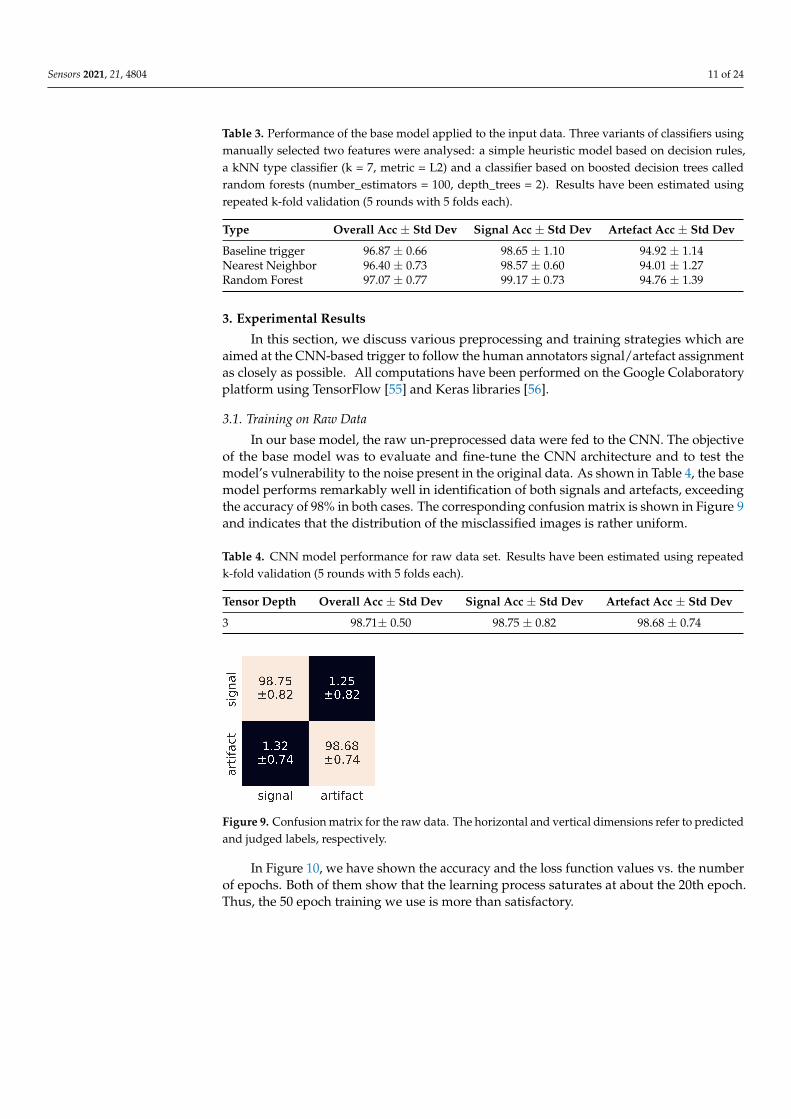
In our base model, the raw un-preprocessed data were fed to the CNN. The objectiveof the base model was to evaluate and fine-tune the CNN architecture and to test themodel’s vulnerability to the noise present in the original data. As shown in Table 4, the basemodel performs remarkably well in identification of both signals and artefacts, exceedingthe accuracy of 98% in both cases. The corresponding confusion matrix is shown in Figure 9and indicates that the distribution of the misclassified images is rather uniform.
Table 4. CNN model performance for raw data set. Results have been estimated using repeatedk-fold validation (5 rounds with 5 folds each).
Tensor Depth Overall Acc ± Std Dev Signal Acc ± Std Dev Artefact Acc ± Std Dev
3 98.71± 0.50 98.75 ± 0.82 98.68 ± 0.74
Figure 9. Confusion matrix for the raw data. The horizontal and vertical dimensions refer to predictedand judged labels, respectively.
In Figure 10, we have shown the accuracy and the loss function values vs. the numberof epochs. Both of them show that the learning process saturates at about the 20th epoch.Thus, the 50 epoch training we use is more than satisfactory.

Sensors 2021, 21, 4804 12 of 24
(a) accuracy plot (b) loss plotFigure 10. CNN model learning history showing accuracy and loss curves. A logarithmic scale has been applied to the lossplot to keep a better visibility.
3.2. Training on Wavelet Transformed Data
In this section, we present the results obtained using the method discussed in Section 2.To select the optimal form of the input to the CNN, apart from the adaptive thresholdingdiscussed in Section 2.3, we tested several types and combinations of Daubechies wavelettransforms available in Mahotas library [57]. In Table 5, we show the recognition accuracyrates for the input signals in the form of a single wavelet (1-dimensional input tensor).All results have been evaluated using the repeated 5-fold cross-validation. Apparently,the application of any type of the wavelet from the set (D2, D4, . . . , D20) results in arecognition rate, for both signals and artefacts, equal to 98% within two standard deviations.
In Table 6, we show the accuracy results obtained with another approach, where theCNN was fed with wavelet tensors of varying depths in the range from D2:D4 (2 wavelets)to D2:D20 (10 wavelets). Again, very stable accuracy at the level of 98% was found acrossvarious wavelet sequences.
We attribute this accuracy stability to the fact that, even though both signals andartefacts are very diverse within their respective classes, there are clear morphologicaldistinctions, e.g., in terms of the number of active pixels, between signals and artefacts.This can be observed by comparison of Figures 4–7.
Table 5. CNN model performance for various single wavelet transformations applied to input data.Results have been estimated using repeated k-fold validation (5 rounds with 5 folds each).
WaveletNumber
TensorDepth
Overall Acc± Std Dev
Signal Acc± Std Dev
Artefact Acc± Std Dev
D2 1 98.56 ± 0.62 98.74 ± 0.80 98.41 ± 0.90D4 1 98.54 ± 0.48 98.51 ± 0.86 98.45 ± 0.99D6 1 98.48 ± 0.46 98.51 ± 0.86 98.45 ± 0.99D8 1 98.48 ± 0.46 98.51 ± 0.86 98.45 ± 0.99D10 1 98.62 ± 0.49 99.01 ± 0.66 98.22 ± 0.78D12 1 98.63 ± 0.49 98.88 ± 0.69 98.34 ± 0.73D14 1 98.53 ± 0.56 98.60 ± 0.91 98.45 ± 0.83D16 1 98.44 ± 0.56 98.60 ± 0.91 98.45 ± 0.83D18 1 98.38 ± 0.40 98.49 ± 0.64 98.25 ± 0.94D20 1 98.28 ± 0.57 98.55 ± 0.83 97.99 ± 1.19

Sensors 2021, 21, 4804 13 of 24
Table 6. CNN model performance for various wavelet transformations applied to input data (deeptensors). Results have been estimated using repeated k-fold validation (5 rounds with 5 folds each).
WaveletsSequence
TensorDepth
Overall Acc± Std Dev
Signal Acc± Std Dev
Artefact Acc± Std Dev
D2:D4 2 98.62 ± 0.41 98.86 ± 0.63 98.36 ± 1.64D2:D6 3 98.65 ± 0.54 98.62 ± 0.77 98.68 ± 0.85D2:D8 4 98.65 ± 0.54 98.62 ± 0.62 98.68 ± 0.92D2:D10 5 98.71 ± 0.49 98.83 ± 0.74 98.57 ± 0.65D2:D12 6 98.60 ± 0.39 98.75 ± 0.85 98.43 ± 0.92D2:D14 7 98.67 ± 0.40 99.01 ± 0.67 98.29 ± 0.76D2:D16 8 98.64 ± 0.50 98.83 ± 0.68 98.43 ± 0.88D2:D18 9 98.73 ± 0.47 98.86 ± 0.83 98.59 ± 0.83D2:D20 10 98.71 ± 0.47 98.73 ± 0.66 98.68 ± 0.73
Finally, in Figure 11 we show confusion matrices, for both single wavelet and waveletsequence versions of the experiment. Again, we see that (within one standard deviation)the misclassification rate is the same for signals and artefacts and is not worse than 2%.
(a) D2 (b) D20 (c) D2:D4 (d) D2:D20Figure 11. Confusion matrices for different input tensors: (a) single D2 wavelet, (b) single D20 wavelet, (c) composition of[D2,D4] wavelets, (d) composition of [D2,D4,D6,...,D20] wavelets. The horizontal and vertical dimensions refer to predictedand judged labels, respectively.
As shown in Figure 12, the CNN learning curves for the wavelet transformed inputstabilise around the 20th epoch.
(a) accuracy plot (b) loss plotFigure 12. The exemplary of CNN model learning history for input tensor consisting of D2:D20 wavelets: (a) accuracy plot,(b) loss curve. A logarithmic scale has been applied to the loss plot to keep a better visibility.

Sensors 2021, 21, 4804 14 of 24
3.3. Combined Approach
Finally, we explored the possibility to feed the CNN with both the raw data as wellas the thresholded and then wavelet transformed data. This way, the model was exposedto effective feature extraction (by the wavelet transform), while retaining the informationof the substantial noise component. Again, as can be observed in Table 7, the recogni-tion rate exceeds 98% but compared to the training on raw data or wavelet transformeddata separately, we do not observe substantial gain in combining the two approaches.The corresponding confusion matrices are shown in Figure 13.
Table 7. CNN model performance for raw data combined with wavelet set. Results have beenestimated using repeated k-fold validation (5 rounds with 5 folds each).
DataSet
TensorDepth
Overall Acc± Std Dev
Signal Acc± Std Dev
Artefact Acc± Std Dev
raw + D2 2 98.93 ± 0.39 98.99 ± 0.63 98.86 ± 0.67raw + D20 2 98.71 ± 0.43 98.64 ± 0.80 98.79 ± 0.64raw + D2:D20 11 98.84 ± 0.55 98.94 ± 0.71 98.73 ± 0.95
(a) raw+D2 (b) raw+D20 (c) raw+D2:D20Figure 13. Confusion matrices for different dimensions of the input tensors: (a) composition of the raw image and single D2wavelet, (b) composition of the raw image and single D20 wavelet, (c) composition of the raw image and collection of [D2,D4, ..., D20] wavelets. The horizontal and vertical dimensions refer to predicted and judged labels, respectively.
Figure 14 indicates that similarly as in previous two cases the CNN learning curvesfor the combined input stabilise around 20th epoch.
(a) accuracy plot (b) loss plotFigure 14. CNN model learning history for an input tensor consisting of raw data merged with D2:20 wavelets: (a) accuracyplot, (b) loss curve. A logarithmic scale has been applied to the loss plot to keep a better visibility.

Sensors 2021, 21, 4804 15 of 24
3.4. Discussion of Experimental Results
The CNN classifier variants introduced in Sections 3.1–3.3 retain the same architecturebut differ in the type and size of the input data. Despite this, their performance is compara-ble to within one standard deviation and achieves an accuracy close to 99%. To ascertainrobustness and stability, verification of the obtained accuracy was performed using thek-fold cross-validation technique. The summary results of the computational experimentsin this regard are given in Tables 4–7. As the performance of the different variants of theclassified do not differ significantly, in practical applications the model with lower timecomplexity should be favoured. The performance estimation of the different variants ofthe proposed classifier in this regard is presented in Table 8. These values indicate that itis worth using models requiring input data of the smallest possible size, i.e., raw imagesor single wavelets. This may be important in applications that require running the modeldirectly on mobile devices (smartphones).
The learning curves shown in Figures 10, 12 and 14 exhibit some perturbations overthe first few epochs. This is particularly strongly visible for models using tensor inputscontaining wavelets. This phenomenon is probably due to rapid changes in model parame-ters during the initial learning phase. This is turn may be a consequence of the relativelysmall depth of the network and the small spatial size of the input images.
Table 8. CNN model timing for different type of input data, where raw denotes the original RGBimage and Dn means Daubechies wavelet with length of n. To obtain statistically reliable results,classification time was measured for 105 samples and then averaged.
Data Set Tensor Depth Learning Time [s]for 50 Epochs
Prediction Time [µs]for Single Image
raw 3 27 100D2 1 29 110raw + D2 4 29 140raw + D2:D10 8 33 180raw + D2:D20 13 39 260
3.5. Demonstration of Models Performance
We want to stress one more time that at the present stage of investigation the onlymeaningful question one may ask in not how accurate the classification is but ratherhow accurately the trigger mimics the human annotators and how consistent it is intriggering. Figures 15 and 16 show the random specimens of 25 images classified as signalsand artefacts. Both figures show, albeit qualitatively, that the trigger is rather consistent.Providing more quantitative support of trigger accuracy requires larger set of annotatedimages. An alternative approach would be to cross check the CNN based trigger with analternative trigger. We are currently performing such a study.

Sensors 2021, 21, 4804 16 of 24
Figure 15. Classification on the selected part of the original CREDO set demonstrating signal class. An example of theperformance of a classifier based on a dimension 2 input tensor composed of the greyscale image and a D2 wavelet.

Sensors 2021, 21, 4804 17 of 24
Figure 16. Classification on the selected part of original CREDO set demonstrating the artefact class. An example of theperformance of a classifier based on a dimension 2 input tensor composed of the greyscale image and a D2 wavelet.
4. Discussion of Alternative Architectures
The main motivation behind the trigger architecture discussed in the preceding sec-tions was to create a solution which, on the one hand, will be able to encompass the greatvariety of signal and artefact morphologies and, on the other hand, will easily generalise(without a change in network structure) to several signal classes. The canonical classesof signals observed in CCDs have been defined almost 20 years ago as spots, tracks andworms [58]. However, later CMOS-based observations, also by CREDO collaboration,suggested the emergence of multi-track signals, so the classifying network must be bigenough to be able to accommodate such extended classification. Furthermore, given the

Sensors 2021, 21, 4804 18 of 24
current CREDO dataset size of several millions of images and its designed increase bytwo orders of magnitude, we have adopted preprocessing operations that are as simpleand time efficient as possible. Therefore, having performed the wavelet transform, werefrained from further image segmentation but rather utilised the CNN’s capability tosimultaneously process several sectors of each image, and then fed the four sub-imagesresulting from Equation (4) as a single image.
Now, it is tempting to check how these two assumptions (flat input and big network)impacted the overall classifier’s performance. To this end we performed two exploratorystudies, discussed in the following two subsections, where we analysed an alternativeinput organisation, and secondly analysed the performance of the CNN with the numberof input parameters reduced by an order of magnitude.
4.1. Alternative Input Organisation
The wavelet transform computed for a single image generates four components (a,v, h, d), with each component being half the size of the original input image. In thebasic solution, these four components are spatially folded into a single image whosedimensions add up to the original image. This technique allows such wavelet subimagesto be combined together with the original image into a single coherent tensor withoutscaling. In this section, we discuss another approach to constructing the input data tensorby treating individual wavelet components as separate layers. The formal definition of thisway of constructing the wavelet representation as a multidimensional tensor is describedby Equation (6).
f→ [a|v|h|d], (6)
where subimage a denotes the average signal while h, v and d denote the horizontal,vertical and diagonal fluctuations, respectively [54].
As a result, the wavelet representation generated for a single image takes the formof a tensor with dimensions half the size of the original image (30 × 30 px) and a depthof 4 layers. As the base model uses a set of transforms chosen in such a way that it canefficiently process input data with a resolution of 60 × 60 px, it is necessary to scale thetwice smaller wavelet representation to this size. Without this rescaling, it would also notbe possible to assemble the input data tensor containing the wavelets and raw image. Therescaling is done by interpolating the individual wavelet images to a higher resolution. Thiskeeps the size of input tensors unchanged and allows a direct comparison of the obtainedclassification results, as the model architecture and the input data size are preserved.
In order to evaluate whether this arrangement of wavelet components noticeablyaffects the classification results, a corresponding experiment was conducted. Input datatensors constructed according to the newly proposed scheme, i.e., sequential arrangementof wavelet components, were loaded into the base classifier discussed in Section 2.2. Thesetensors were also supplemented with an additional layer in the form of a greyscale imageto enrich information about the global luminance distribution. The results obtained areshown in Table 9. They are comparable in terms of standard deviation accuracy with thepreviously obtained results for the base model. Thus, there is no noticeable effect of thewavelet component setting on the model performance.
4.2. Application of Smaller Scale Model
Besides the input data format, the second extremely important aspect is the modelarchitecture itself. The proposed base model by its scale far exceeds the size of the learningset. The model itself is not very deep (4 convolutional layers), but it is quite broad in thesense that it uses a significant number of filters in each layer. This results in a model sizeof about 1 million parameters requiring learning and tuning. Compared to the size of thetraining set, which contains about 2000 elements, there may be reasonable doubt as to

Sensors 2021, 21, 4804 19 of 24
whether such a difference in scale compromises the ability to effectively learn such a modelfrom the available data.
Table 9. Base CNN model performance for various single wavelet transformations applied to inputdata. Input tensor composed of a greyscale image and wavelet image components (a, v, h, d) set ina sequence which gives a tensor depth of 1 + 4. Results have been estimated using repeated k-foldvalidation (5 rounds with 5 folds each).
WaveletNumber
TensorDepth
Overall Acc± Std Dev
Signal Acc± Std Dev
Artefact Acc± Std Dev
raw + D2 5 98.11 ± 0.61 97.92 ± 0.91 98.32 ± 1.09raw + D4 5 98.10 ± 0.49 97.71 ± 0.86 98.54 ± 0.66raw + D6 5 97.92 ± 0.69 97.84 ± 0.96 97.90 ± 1.17raw + D8 5 97.99 ± 0.56 97.95 ± 1.01 98.02 ± 1.11raw + D10 5 98.03 ± 0.55 98.02 ± 0.96 98.04 ± 0.91raw + D12 5 98.10 ± 0.65 97.79 ± 1.06 98.43 ± 0.89raw + D14 5 98.10 ± 0.57 98.26 ± 0.85 97.90 ± 0.81raw + D16 5 98.13 ± 0.52 98.18 ± 0.58 98.07 ± 0.97raw + D18 5 97.95 ± 0.56 97.97 ± 0.78 97.93 ± 1.23raw + D20 5 98.04 ± 0.46 98.07 ± 0.70 98.00 ± 0.73
To verify this issue, a dedicated smaller scale model was developed for comparisonpurposes. During the development of the small scale model, it became apparent thatit needed to be much deeper than the base model in order to learn effectively from theavailable data. The result of many design trials and experiments is the architecture of theconvolutional network shown in Table 10 and in illustrative form in Figure 17. The finalmodel has about 100,000 parameters requiring learning and tuning, so it is an order ofmagnitude smaller than the baseline model. Consequently, this model should be lesssusceptible to overfitting than the baseline model.
Figure 17. Layer-oriented signal flow in the convolutional network (CNN) artefact filtration model of a smaller scale.
This small-scale model was then trained on a standard dataset to compare the perfor-mance and statistical parameters of the classification process with that of the base model.To this end, both of the wavelet tensor ordering techniques discussed previously wereused, i.e., combining subimages of a single layer and combining subimages into a sequenceof layers. In addition, in both cases the tensor was extended with a layer containing thegreyscale source image. Tables 11 and 12 present the obtained wavelet tensor classificationresults ordered according to the schemes described by Formulas (4) and (6), respectively.

Sensors 2021, 21, 4804 20 of 24
Table 10. Layer-by-layer summary of the proposed smaller-scale CNN model. Each layer nameis given followed by the number of feature maps (convolutional layers) or neurons (dense layers),the size of the convolutional filter or pooling region, the activation function used and, last, the numberof parameters to learn.
Layer Type Features Size Activation Params
Convolution 2D 16 3 × 3 ReLU 736Convolution 2D 16 5 × 5 ReLU 6416Max Pooling - 2 × 2 - -Convolution 2D 16 3 × 3 ReLU 2320Convolution 2D 16 3 × 3 ReLU 2320Convolution 2D 16 5 × 5 ReLU 6416Max Pooling - 2 ×2 - -Convolution 2D 16 3 × 3 ReLU 2320Convolution 2D 16 3 × 3 ReLU 2320Convolution 2D 16 5 × 5 ReLU 6416Max Pooling - 2 × 2 - -Convolution 2D 16 3 × 3 ReLU 2320Convolution 2D 16 3 × 3 ReLU 2320Convolution 2D 16 5 × 5 ReLU 6416Max Pooling - 2 × 2 - -
Flatten 144 - - -
Dense 300 - ReLU 43,500Dense 50 - ReLU 15,050
Dense 2 - Softmax 102TOTAL PARAMS: 98,972TRAINABLE PARAMS: 98,972NON-TRAINABLE PARAMS: 0
Table 11. Smaller-scale CNN model performance for various single wavelet transformations ap-plied to input data. Results have been estimated using repeated k-fold validation (5 rounds with5 folds each).
WaveletNumber
TensorDepth
Overall Acc± Std Dev
Signal Acc± Std Dev
Artefact Acc± Std Dev
raw + D2 2 98.33 ± 0.58 98.49 ± 0.67 98.15 ± 1.14raw + D4 2 98.12 ± 0.88 98.33 ± 1.02 97.90 ± 1.22raw + D6 2 98.26 ± 0.48 98.41 ± 0.69 98.09 ± 0.89raw + D8 2 98.38 ± 0.60 98.46 ± 1.08 98.29 ± 0.80raw + D10 2 98.27 ± 0.48 98.59 ± 0.65 97.91 ± 0.84raw + D12 2 98.30 ± 0.61 98.52 ± 0.82 98.06 ± 1.06raw + D14 2 98.13 ± 0.55 98.28 ± 0.71 97.97 ± 0.96raw + D16 2 98.18 ± 0.53 98.36 ± 0.86 97.99 ± 0.89raw + D18 2 98.14 ± 0.57 98.10 ± 0.98 98.18 ± 0.85raw + D20 2 98.17 ± 0.54 98.30 ± 0.83 98.04 ± 0.73
Comparing the classification results obtained with the base model and the small-scalemodel, it cannot be concluded that they differ significantly from each other. With respect tothe determined standard deviations, the analysed models show comparable performance.Thus, in our opinion, it can be concluded that the use of the base model is justified even inthe case of a large scale difference with respect to the power of the available training set.
A baseline model using an architecture with more learning parameters certainly hasmuch more potential in terms of discriminative ability and intrinsic feature representation

Sensors 2021, 21, 4804 21 of 24
capacity. In this sense, it may be promising to use it as a prototype solution for moredemanding applications, such as multi-class classification of signals distinguishing theirdifferent morphologies.
Table 12. Smaller-scale CNN model performance for various single wavelet transformations appliedto input data. Input tensor composed of a greyscale image and wavelet image components (a, v, h, d)set in a sequence which gives a tensor depth of 1 + 4. Results have been estimated using repeatedk-fold validation (5 rounds with 5 folds each).
WaveletNumber
TensorDepth
Overall Acc± Std Dev
Signal Acc± Std Dev
Artefact Acc± Std Dev
raw + D2 5 98.16 ± 0.54 98.10 ± 0.88 98.22 ± 0.89raw + D4 5 98.10 ± 0.48 98.02 ± 0.82 98.20 ± 0.84raw + D6 5 97.99 ± 0.54 97.99 ± 0.88 98.00 ± 1.10raw + D8 5 98.02 ± 0.35 97.89 ± 0.93 98.18 ± 0.94raw + D10 5 97.87 ± 0.64 97.74 ± 0.97 98.00 ± 0.92raw + D12 5 97.91 ± 0.69 97.82 ± 1.05 98.00 ± 0.86raw + D14 5 97.82 ± 0.61 97.94 ± 1.08 97.68 ± 1.11raw + D16 5 97.99 ± 0.58 98.04 ± 0.99 97.95 ± 0.96raw + D18 5 97.99 ± 0.42 97.68 ± 1.12 97.91 ± 1.10raw + D20 5 97.86 ± 0.59 97.79 ± 1.03 97.93 ± 0.86
4.3. Summary of Alternative Architectures
To summarise our exploratory studies towards modified shape of the input tensor andthe decreased number of CNN’s units, we conclude neither replacing the single waveletimage with a tensor dimension equal to four nor the decrease of the number of neuronsby one order of magnitude do not change significantly the classifier’s performance. Thus,given the original requirements of fast image preprocessing and the network’s ability toaccommodate multi-class classification, we conclude that the original trigger setup is theright base for larger dataset trigger.
5. Summary and Outlook
We described an application of a Convolutional Neural Network to filter artefactsin the cosmic ray detection experiments performed on mobile phones. Generally, suchexperiments are aimed at broader scientifically oriented audience, in the framework of theso called Citizen Science philosophy. A gamification (e.g., Particle Hunters’ Competitions)is an efficient method to sustain the participants’ engagement, necessary for such projectsto be scientifically productive. However, the gamification is accompanied by the surgeof fake signals related either to the hardware malfunction or participants’ cheating. Ourmethod uses a subset of CREDO images labelled by judges as either “signal” or “artefact”.We started from considering a baseline trigger whose training consisted on constructingthe decision boundary in two-dimensional feature space defined by integrated luminositiesand the number of active pixels. On average the baseline trigger and its refined versionsbased on kNN and RF classifiers performed just 2% worse than the CNN trigger. Theirartefact recognition rate was, however, 4% worse than that of the CNN trigger. Then, wehave studied three versions of the experiment setup and two architectures of CNN models.In the basic version, the raw CR images were fed to the CNN. In the refined versionof our solution, the images were adaptively thresholded and then subject to wavelettransforms. The motivation of the wavelet transform was its ability to amplify distinctivesignal features, like the shape of object borders or its fragmentation. Such input wasthen fed to the CNN. Finally, we have studied the impact of simultaneous feeding of rawand wavelet transformed data but found no significant improvement of the recognitionrate. The overall accuracy of three discussed approaches reached the level of 98–99% forboth signal and artefacts. With such accuracies the adverse effects of gamification can be

Sensors 2021, 21, 4804 22 of 24
effectively neutralised. Given the similar performance of all three preprocessing methodsthe practical application of the method is determined by time efficiency which favours theraw RGB based CNN classification.
In general, the classifiers investigated are limited to some extent by the accuracy of theannotators in recognising whether a hit is a signal or artefact. As shown in the paper, CNNtriggers were found to be significantly more consistent than annotators (smaller standarddeviation). The natural extension of the presented methods is to increase the number ofsignal classes so that various types of particle tracks can be identified. This research iscurrently under way.
Author Contributions: Conceptualisation, M.P. (Marcin Piekarczyk), K.R. and Ł.B.; methodol-ogy, M.P. (Marcin Piekarczyk) and K.R.; software, M.P. (Marcin Piekarczyk) and O.B.; validation,M.P. (Marcin Piekarczyk), Ł.B., K.R., O.B., S.S. and M.N.; formal analysis, Ł.B.; investigation, M.P.(Marcin Piekarczyk); resources, S.S. and M.N.; data curation, S.S. and M.N.; writing—original draftpreparation, M.P. (Marcin Piekarczyk), Ł.B., K.R., O.B., S.S., T.A. and M.N.; writing—review andediting, N.M.B., D.E.A.-C., K.A.C., D.G., A.C.G., B.H., P.H., R.K., M.K. (Marcin Kasztelan), M.K.(Marek Knap), P.K., B.Ł., J.M., A.M., V.N., M.P. (Maciej Pawlik), M.R., O.S., K.S. (Katarzyna Smelcerz),K.S. (Karel Smolek), J.S., T.W., K.W.W., J.Z.-S. and T.A.; visualisation, O.B., M.N. and S.S.; supervision,M.P. (Marcin Piekarczyk) and Ł.B.; project administration, P.H., Ł.B. and M.P. (Marcin Piekarczyk);funding acquisition, P.H., M.P. (Marcin Piekarczyk) and Ł.B. All authors have read and agreed to thepublished version of the manuscript.
Funding: This research was funded under the Pedagogical University of Krakow statutory researchgrant, which was funded by subsidies for science granted by the Polish Ministry of Science andHigher Education. This research was partly funded by the International Visegrad grant No. 21920298.This research has been supported in part by PLGrid Infrastructure and we warmly thank the staff atACC Cyfronet AGH-UST for their always helpful supercomputing support. K.Rz. acknowledgesthat this scientific work was partly supported by the AGH University of Science and Technology inthe year 2021 as research project No. 16.16.120.773.
Institutional Review Board Statement: Not applicable.
Informed Consent Statement: Not applicable.
Data Availability Statement: The training set as well as the source code used in this analysis areavailable at https://github.com/credo-ml/cnn-offline-trigger, accessed on 9 July 2021.
Conflicts of Interest: The authors declare no conflicts of interest.
AbbreviationsThe following abbreviations are used in this manuscript:
CREDO Cosmic Ray Extremely Distributed ObservatoryCNN Convolutional Neural NetworkRNN Recurrent Neural NetworksGNN Graph Neural NetworksReLU Rectified Linear UnitANN Artificial Neural NetworkSVM Support Vector MachineRF Random ForestDECO Distributed Electronic Cosmic-ray ObservatoryCCD Charge Coupled DeviceCMOS Complementary Metal-Oxide-SemiconductorCRAYFIS Cosmic RAYs Found In Smartphones
References1. Homola, P.; Beznosko, D.; Bhatta, G.; Bibrzycki, Ł.; Borczynska, M.; Bratek, Ł.; Budnev, N.; Burakowski, D.; Alvarez-Castillo, D.E.;
Almeida Cheminant, K.; et al. Cosmic-Ray Extremely Distributed Observatory. Symmetry 2020, 12, 1835. [CrossRef]2. Unger, M.; Farrar, G. (In) Feasability of Studying Ultra-High-Energy Cosmic Rays with Smartphones. arXiv 2015, arXiv:1505.04777.

Sensors 2021, 21, 4804 23 of 24
3. Kumar, R. Tracking Cosmic Rays by CRAYFIS (Cosmic Rays Found in Smartphones) Global Detector. In Proceedings of the 34thInternational Cosmic Ray Conference (ICRC2015), Hague, The Netherlands, 30 July–6 August 2015; Volume 34, p. 1234.
4. Borisyak, M.; Usvyatsov, M.; Mulhearn, M.; Shimmin, C.; Ustyuzhanin, A. Muon trigger for mobile phones. J. Phys. 2017, 898,032048. [CrossRef]
5. Albin, E.; Whiteson, D. Feasibility of Correlated Extensive Air Shower Detection with a Distributed Cosmic Ray Network. arXiv2021, arXiv:2102.03466.
6. Whiteson, D.; Mulhearn, M.; Shimmin, C.; Cranmer, K.; Brodie, K.; Burns, D. Searching for ultra-high energy cosmic rays withsmartphones. Astropart. Phys. 2016, 79, 1–9. [CrossRef]
7. Winter, M.; Bourbeau, J.; Bravo, S.; Campos, F.; Meehan, M.; Peacock, J.; Ruggles, T.; Schneider, C.; Simons, A.L.; Vandenbroucke,J. Particle identification in camera image sensors using computer vision. Astropart. Phys. 2019, 104, 42–53. [CrossRef]
8. Vandenbroucke, J.; Bravo, S.; Karn, P.; Meehan, M.; Plewa, M.; Ruggles, T.; Schultz, D.; Peacock, J.; Simons, A.L. Detectingparticles with cell phones: The Distributed Electronic Cosmic-ray Observatory. arXiv 2015, arXiv:1510.07665.
9. Vandenbroucke, J.; BenZvi, S.; Bravo, S.; Jensen, K.; Karn, P.; Meehan, M.; Peacock, J.; Plewa, M.; Ruggles, T.; Santander, M.; et al.Measurement of cosmic-ray muons with the Distributed Electronic Cosmic-ray Observatory, a network of smartphones. J. Instrum.2016, 11, 04019. [CrossRef]
10. Meehan, M.; Bravo, S.; Campos, F.; Peacock, J.; Ruggles, T.; Schneider, C.; Simons, A.L.; Vandenbroucke, J.; Winter, M. The particledetector in your pocket: The Distributed Electronic Cosmic-ray Observatory. arXiv 2017, arXiv:1708.01281.
11. De Angelis, A.; Pimenta, M. Introduction to Particle and Astroparticle Physics; Springer: Cham, Swizerland; London, UK, 2018.12. Collaboration, H.; Abramowski, A.; Aharonian, F. Acceleration of petaelectronvolt protons in the Galactic Centre. Nature 2016,
531, 476–479. [CrossRef]13. Webb, G.M.; Al-Nussirat, S.; Mostafavi, P.; Barghouty, A.F.; Li, G.; le Roux, J.A.; Zank, G.P. Particle Acceleration by Cosmic Ray
Viscosity in Radio-jet Shear Flows. Astrophys. J. 2019, 881, 123. [CrossRef]14. Globus, N.; Blandford, R.D. The Chiral Puzzle of Life. Astrophys. J. 2020, 895, L11. [CrossRef]15. Catalogue of electron precipitation events as observed in the long-duration cosmic ray balloon experiment. J. Atmos. Sol. Terr.
Phys. 2016, 149, 258–276. [CrossRef]16. Chancellor, J.C.; Scott, G.B.I.; Sutton, J.P. Space Radiation: The Number One Risk to Astronaut Health beyond Low Earth Orbit.
Life 2014, 4, 491–510. [CrossRef]17. Mavromichalaki, H.; Papailiou, M.; Dimitrova, S.; Babayev, E.S.; Loucas, P. Space weather hazards and their impact on human
cardio-health state parameters on Earth. Nat. Hazards 2012, 64, 1447–1459. [CrossRef]18. The CREDO Collaboration. CREDO Detector. 2021. Available online: https://github.com/credo-science/credo-detector-android
(accessed on 27 January 2021).19. Bibrzycki, Ł.; Burakowski, D.; Homola, P.; Piekarczyk, M.; Niedzwiecki, M.; Rzecki, K.; Stuglik, S.; Tursunov, A.; Hnatyk, B.;
Castillo, D.E.A.; et al. Towards A Global Cosmic Ray Sensor Network: CREDO Detector as the First Open-Source MobileApplication Enabling Detection of Penetrating Radiation. Symmetry 2020, 12, 1802. [CrossRef]
20. Particle Hunters—CREDO Competition. Available online: https://credo.science/particle_hunters/) (accessed on 9 July 2021).21. Murphy, K.P. Machine Learning: A Probabilistic Perspective, 1st ed.; Adaptive Computation and Machine Learning; The MIT Press:
Cambridge, MA, USA, 2012.22. James, G.; Witten, D.; Hastie, T.; Tibshirani, R. An Introduction to Statistical Learning: With Applications in R; Springer Publishing
Company, Incorporated: Berlin/Heidelberg, Germany, 2014.23. Cortes, C.; Vapnik, V. Support-vector networks. Mach. Learn. 1995, 20, 273–297. [CrossRef]24. Ripley, B.D. Pattern Recognition and Neural Networks; Cambridge University Press: Cambridge, UK, 2007.25. Biau, G.; Scornet, E. A random forest guided tour. Test 2016, 25, 197–227. [CrossRef]26. Li, Z.; Yang, W.; Peng, S.; Liu, F. A survey of convolutional neural networks: Analysis, applications, and prospects. arXiv 2020,
arXiv:2004.02806.27. Ghatak, A. Recurrent neural networks (RNN) or sequence models. In Deep Learning with R; Springer: Berlin/Heidelberg,
Germany, 2019; pp. 207–237.28. Wu, Z.; Pan, S.; Chen, F.; Long, G.; Zhang, C.; Philip, S.Y. A comprehensive survey on graph neural networks. IEEE Trans. Neural
Netw. Learn. Syst. 2020, 32, 4–24. [CrossRef]29. Yaneva, V.; Eraslan, S.; Yesilada, Y.; Mitkov, R. Detecting high-functioning autism in adults using eye tracking and machine
learning. IEEE Trans. Neural Syst. Rehabil. Eng. 2020, 28, 1254–1261. [CrossRef]30. Mekov, E.; Miravitlles, M.; Petkov, R. Artificial intelligence and machine learning in respiratory medicine. Expert Rev. Respir. Med.
2020, 14, 559–564. [CrossRef] [PubMed]31. Huang, K.; Bryant, T.; Schneider, B. Identifying Collaborative Learning States Using Unsupervised Machine Learning on
Eye-Tracking, Physiological and Motion Sensor Data. In Proceedings of the 12th International Conference on Educational Data,Montreal, QC, Canada, 2–5 July 2019; pp. 318–332.
32. Sharma, K.; Giannakos, M.; Dillenbourg, P. Eye-tracking and artificial intelligence to enhance motivation and learning. SmartLearn. Environ. 2020, 7, 1–19. [CrossRef]
33. Tomczyk, K.; Piekarczyk, M.; Sieja, M.; Sokal, G. Special functions for the extended calibration of charge-mode accelerometers.Precis. Eng. 2021, 71, 153–169. [CrossRef]

Sensors 2021, 21, 4804 24 of 24
34. Tomczyk, K.; Piekarczyk, M.; Sokal, G. Radial basis functions intended to determine the upper bound of absolute dynamic errorat the output of voltage-mode accelerometers. Sensors 2019, 19, 4154. [CrossRef] [PubMed]
35. Wang, L.; Wang, Y. Application of Machine Learning for Process Control in Semiconductor Manufacturing. In Proceedings ofthe 2020 International Conference on Internet Computing for Science and Engineering, Meemu Atoll, Maldive, 14–16 July 2020;pp. 109–111.
36. Bibi, K.; Naz, S.; Rehman, A. Biometric signature authentication using machine learning techniques: Current trends, challengesand opportunities. Multimed. Tools Appl. 2020, 79, 289–340. [CrossRef]
37. Kim, S.K.; Yeun, C.Y.; Damiani, E.; Lo, N.W. A machine learning framework for biometric authentication using electrocardiogram.IEEE Access 2019, 7, 94858–94868. [CrossRef]
38. Wójcik, K.; Piekarczyk, M. Machine Learning Methodology in a System Applying the Adaptive Strategy for Teaching HumanMotions. Sensors 2020, 20, 314. [CrossRef]
39. Fang, B.; Jia, S.; Guo, D.; Xu, M.; Wen, S.; Sun, F. Survey of imitation learning for robotic manipulation. Int. J. Intell. Robot. Appl.2019, 3, 362–369. [CrossRef]
40. Hachaj, T.; Piekarczyk, M. Evaluation of pattern recognition methods for head gesture-based interface of a virtual reality helmetequipped with a single IMU sensor. Sensors 2019, 19, 5408. [CrossRef]
41. Nogales, R.; Benalcázar, M.E. A survey on hand gesture recognition using machine learning and infrared information. InInternational Conference on Applied Technologies; Springer: Berlin/Heidelberg, Germany, 2019; pp. 297–311.
42. Krizhevsky, A.; Sutskever, I.; Hinton, G.E. Imagenet classification with deep convolutional neural networks. Adv. Neural Inf.Process. Syst. 2012, 25, 1097–1105. [CrossRef]
43. He, K.; Zhang, X.; Ren, S.; Sun, J. Deep Residual Learning for Image Recognition. arXiv 2015, arXiv:cs.CV/1512.03385.44. Chollet, F. Xception: Deep learning with depthwise separable convolutions. In Proceedings of the IEEE Conference on Computer
Vision and Pattern Recognition, Honolulu, HI, USA, 21–26 July 2017; pp. 1251–1258.45. Huang, G.; Liu, Z.; Van Der Maaten, L.; Weinberger, K.Q. Densely connected convolutional networks. In Proceedings of the IEEE
Conference on Computer Vision and Pattern Recognition, Honolulu, HI, USA, 21–26 July 2017; pp. 4700–4708.46. Simonyan, K.; Zisserman, A. Very deep convolutional networks for large-scale image recognition. arXiv 2014, arXiv:1409.1556.47. Sandler, M.; Howard, A.; Zhu, M.; Zhmoginov, A.; Chen, L.C. Mobilenetv2: Inverted residuals and linear bottlenecks. In
Proceedings of the IEEE Conference on Computer Vision and Pattern Recognition, Salt Lake City, UT, USA, 18–23 June 2018;pp. 4510–4520.
48. Russakovsky, O.; Deng, J.; Su, H.; Krause, J.; Satheesh, S.; Ma, S.; Huang, Z.; Karpathy, A.; Khosla, A.; Bernstein, M.; et al.Imagenet large scale visual recognition challenge. Int. J. Comput. Vis. 2015, 115, 211–252. [CrossRef]
49. Hachaj, T.; Bibrzycki, Ł.; Piekarczyk, M. Recognition of Cosmic Ray Images Obtained from CMOS Sensors Used in Mobile Phonesby Approximation of Uncertain Class Assignment with Deep Convolutional Neural Network. Sensors 2021, 21, 1963. [CrossRef][PubMed]
50. Niedzwiecki, M.; Rzecki, K.; Marek, M.; Homola, P.; Smelcerz, K.; Castillo, D.A.; Smolek, K.; Hnatyk, B.; Zamora-Saa, J.;Mozgova, A.; et al. Recognition and classification of the cosmic-ray events in images captured by CMOS/CCD cameras. arXiv2019, arXiv:astro-ph.IM/1909.01929.
51. Niedzwiecki, M. Manual Classification of CREDO Cosmic Ray Traces. 2021. Available online: https://credo.nkg-mn.com/(accessed on 2 February 2021).
52. Hinton, G.; Srivastava, N.; Swersky, K. Neural networks for machine learning lecture 6a overview of mini-batch gradient descent.Cited 2012, 14, 2.
53. Zou, H.; Hastie, T. Regularization and variable selection via the elastic net. J. R. Stat. Soc. Ser. B 2005, 67, 301–320. [CrossRef]54. Walker, J. A Primer on Wavelets and Their Scientific Applications; CRC Press: Boca Raton, FL, USA, 1999.55. Abadi, M.; Agarwal, A.; Barham, P.; Brevdo, E.; Chen, Z.; Citro, C.; Corrado, G.S.; Davis, A.; Dean, J.; Devin, M.; et al. TensorFlow:
Large-Scale Machine Learning on Heterogeneous Systems. 2015. Available online: http://tensorflow.org (accessed on 9 July 2021).56. Chollet, F. Keras. 2015. Available online: https://github.com/fchollet/keras (accessed on 9 July 2021).57. Coelho, L. Mahotas: Open source software for scriptable computer vision. J. Open Res. Softw. 2013, 1. [CrossRef]58. Groom, D. Cosmic rays and other nonsense in astronomical CCD imagers. Exp. Astron. 2002, 14, 45–55. [CrossRef]


![International Journal of Engineering Applied Sciences and ...Tesma408,IJEAST.pdf · Glavan and Holban [18] have proposed a convolution neural network (CNN) based pixel classifier](https://img.pdfslide.us/doc/110x75/5f04d2967e708231d40fe1d1/international-journal-of-engineering-applied-sciences-and-tesma408ijeastpdf.jpg)