CMU Strategic Computing Vision Project Report: 1984 to 1985

Takeo Kanade and Charles Thorpe with contributions from

CMU SCVision Project Staff

CMU-RI-TR-86-2

The Robotics Institute Carnegie-Mellon University

Pittsburgh, Pennsylvania 15213

November 1985

Copyright @ 1986 Carnegie-Mellon University

This research was supported in part by the U.S. Army Engineer Topographic Laboratories, under contract number DACA76-85-C-0003,

i

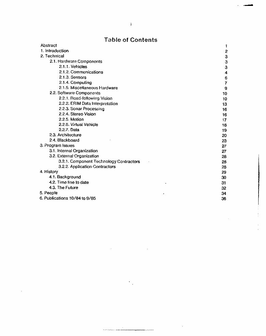
Table of Contents Abstract 1. Introduction 2. Technical

2.1, Hardware Components 2.1.1. Vehicles 2.1.2. Communications 2.1.3. Sensors 2.1.4. Computing 2.1.5. Miscellaneous Hardware

2.2. Software Components 2.2.1. Road-following Vision 2.2.2. ERlM Data Interpretation 2.2.3. Sonar Processing 2.2.4. Stereo Vision 2.2.5. Motion 2.2.6. Virtual Vehicle 2.2.7. Data

2.3. Architecture 2.4. Blackboard

3.1. Internal Organization 3.2. External Organization

3. Program lssiies

3.2.1. Component Technology Contractors 3.2.2. Application Contractors

4. History 4.1. Background 4.2. Time line to date 4.3. The Future

5. People 6. Publications 10/84 to 9/85

1 2 3 3 3 4 6 7 9

10 10 13 16 16 17

19 20 23 27 27

28

29 30 31 32 34 36

i a

28

28

ii

List of Figures

Figure : Terregator and Neptune Figure 2: An oriented edge operator Figure 3: Road tracking with oriented edge operator Figure 4: Road segments and intersection labeled by color classification Figure 5: ERlM processing. From top: range image of traffic cones, navigable

smooth surfaces, detected obstacles. Figure 6: A two-dimensional sonar map. Empty areas with a high certainty factor

are represented by white areas; lower certainty factors by 'I + 'I symbols of increasing thickness. Occupied areas represented by "x" symbols, and Unknown areas by " e " . The position of the robot is shown by acircle and the outline of the room and of the major objects by a solid line.

Figure 7: Levels in the CMU system architecture Figure 8: The local map level Figure 9: Blackboard software configuration Figure 10: Example of a token matching a spec Figure 1 1 : Dialogue model for December map and planning demo

5 11 12 14 15

17

21 22 24 26 33

1

Abstract This report describes work during the first year of CMU’s Strategic Computing Vision project. Our

goal is to build an intelligent mobile robot capable of operating in the real world outdoors. We are approaching this problem by building experimental robot vehicles and software. Experiments in the first year have demonstrated vehicle guidance using sonar, stereo and monoscopic TV cameras, and a laser scanner. This report describes the technical contributions, our relationship with the OARPA Autonomous Land Vehicle project, our project history, the people who comprise our project, and a list of project publications over the last year.

2

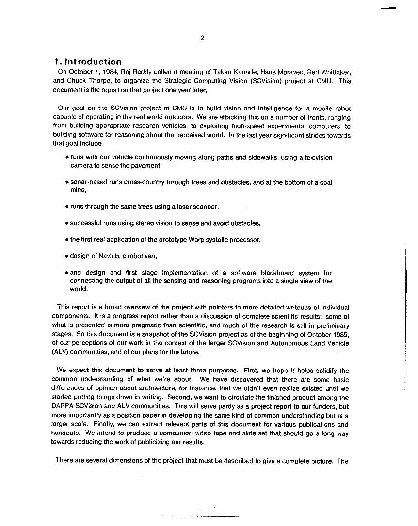
1. Introduction On October 1, 1984, Raj Reddy called a meeting of Takeo Kanade, Hans Moravec, Red Whittaker,

and Chuck Thorpe, to organize the Strategic Computing Vision (SCVision) project at CMU. This document is the report on that project one year later.

Our goal on the SCVision project at CMU is to build vision and intelligence for a mobile robot capable of operating in the real world outdoors. We are attacking this on a number of fronts, ranging from building appropriate research vehicles, to exploiting high-speed experimental computers, to building software for reasoning about the perceived world. In the last year significant strides towards that goal include

0 runs with our vehicle continuously moving along paths and sidewalks, using a television camera to sense the pavement,

0 sonar-based runs cross-country through trees and obstacles, and at the bottom of a coal mine,

0 runs through the same trees using a laser scanner,

0 successful runs using stereo vision to sense and avoid obstacles,

0 the first real application of the prototype Warp systolic processor,

0 design of Navlab, a robot van,

0 and design and first stage implementation of a software blackboard system for connecting the output of all the sensing and reasoning programs into a single view of the world.

This report is a broad overview of the project with pointers to more detailed writeups of individual components. It is a progress report rather than a discussion of complete scientific results: some of what is presented is more pragmatic than scientific, and much of the research is still in preliminary stages. So this document is a snapshot of the SCVision project as of the beginning of October 1985, of our perceptions of our work in, the context of the larger SCVision and Autonomous Land Vehicle (ALV) communities, and of our plans for the future.

We expect this document to serve at least three purposes. First, we hope it helps solidify the common understanding of what we’re about. We have discovered that there are some basic differences of opinion about architecture, for instance, that we didn’t even realize existed until we started putting things down in writing. Second, we want to circulate the finished product among the DARPA SCVision and ALV communities. This will serve partly as a project report to our funders, but more importantly as a position paper in developing the same kind of common understanding but at a larger scale. Finally, we can extract relevant parts of this document for various publications and handouts. We intend to produce a companion video tape and slide set that should go a long way towards reducing the work of publicizing our results.

There are several dimensions of the project that must be described to give a complete picture. The

3

next section of the report describes the technical approach we are taking and the resiilts to date. Section three discusses program issues: how our work fits with the other contractors working on aspects of SCVision and the ALV. The fourth section is a chronolojy of our project, giving background, a time line, and future plans. Our successes are due to hard work by dedicated people, some of whom are listed in section five. Finally, section six is a list of project publications during the past year.

2. Technical Our technical work can be grouped into four main categories:

0 Hardware components of the system

0 Software components

0 Architecture of the system, a blueprint showing how we expect to assemble all the pieces

The Blackboard, which is the mechanism for data fusion

2.1. Hardware Components

2.1 .l. Vehicles The workhorse of the CMU SCVision project has been the Terregator, designed and built by the Civil

Engineering robot lab. We have made occasional use of Neptune, a smaller robot built in the Mobile Robot Lab. We have begun to design Navlab, our Navigation Laboratory of the future. It will be based on a Chevy Van, and will include room for onboard computing and researchers.

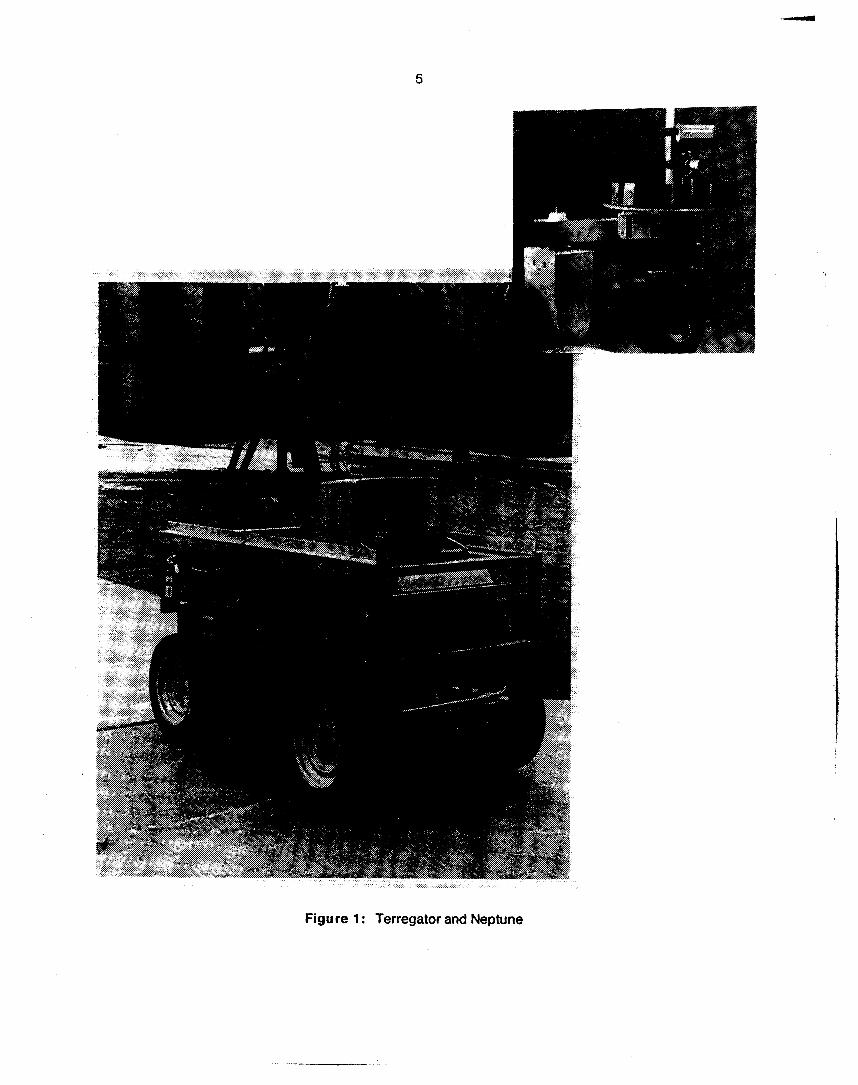
No mobile robot project is complete without a mobile robot. We were extremely fortunate to have had the Terregator built for another project prior to ours. When the previous project completed, we were able to take over the Terregator for our use, and have been relying on it for almost all our mobile robot runs. The Terregator is designed to provide a clean separation between the vehicle itself and its sensor payload. The vehicle provides a mobile platform, power, a 2-way radio for communications with a remote computer, and built in motion commands. Th.is makes it easy for researchers working with different sensor packages to bolt on their choice of sensors, processors, and communications gear, and run their experiments without concern for the details of the vehicle. Details of the terregator are reported by Whittaker [21].

Neptune is a small tethered tricycle designed to provide basic mobility, indoors or on smooth outdoor terrain, for sensor payloads. Its front wheel is steered and driven by a pair of constant-speed AC motors, while its rear wheels are passive. It was designed and built in January through March 1984, and was used for the stereo vision and sonar projects, both indoors and outdoors, for many months before the SCVision project started. Even after the Terregator became available, Neptune has continued to be useful for occasional indoor runs. It is limited by its small payload, its tether, and especially its constant speed motors that prohibit slowing down the vehicle to match our computation speed. For more information on Neptune, see Podnar [12]; see also Moravec [9] and Podnar [ l l ] for discussions of Pluto and Uranus, Neptune’s stable mates in the Mobile Robot Lab.

4

Although we have had good service from Neptune and especially the Terregator, several concerns have prompted the design of a more ambitious research vehicle, the Navlab. The Terregator, in particular, was designed for a different set of missions than those for which we are using it. The original design constraints were for powerful go-anywhere locomotion at slow speeds. The resulting design, with skid steering, is very aggressive, capable of climbing stairs (even trees) and bouncing across railroad tracks, as it has shown in its coal mine run. The side effects, however, are that turns are hard on the grass (an important consideration when we run in a public park) and are somewhat indeterminate. A conventionally-steered vehicle would suit our purposes better. Also, our work over the last year has shown that some of the most interesting problems are in combining the interpretations of several sensors into a single model of the world. While the Terregator can accommodate a single sensor and some sensor combinations, we run out of deck space and electrical power when we try to run several sensors, panltilt mounts, telecommunications, and the vehicle drive motors all at once. Finally, we have found it very helpful to have the computing close to the vehicles. Not only does this reduce the frustrating problems of sending data over a radio link, through trees and buildings and over hills, but it also allows much quicker program/test/debug cycles and cuts down the number of people needed to field a vehicle.

All of the above concerns have led us to the design of Navlab, a Chew van converted into a robot. If funded and built, Navlab will carry stereo TV cameras, a laser scanner, sonars, several computers (both built-in for control and reconfigurable for experiments), and four on-board researchers.

2.1.2. Communications Until we can put powerful computers directly on the vehicle, we must have some sort of

communications link between the robot and the base station. Even a vehicle that carries its processing with it, such as the Navlab, will still want to communicate with delicate or bulky experimental processors and with large archival disk storage. We have steadily improved our communications links from the early days of snowy signals and hard lines.

The Terregator comes complete with a 1200 Baud full duplex radio modem for communicating with its onboard control computer. We have tried different vendors and configurations for the link, and the one that works best is built by Vectran Corporation. It is totally transparent to the computers at either end of it, acting as a standard RS-232 connection. Internally, it does some error detection and retransmission, but the amount of lag time and indeterminacy introduced by that is small.

A second kind of link is for getting video data back from the vehicle. For several months we used a microwave link. This was not an ideal match: the microwave was designed (and licensed) for indoor line of sight use, and was intended for Uranus, the latest progeny of the Mobile Robot Lab. It has a very directional receiving antenna, does not do well penetrating leaves or tree trunks or people, and has a much broader bandwidth (10 MHz) than we need. To make it work, we mounted the receiving antenna and a television camera on a remote-controlled panltilt head, so someone helping with the run could watch the camera and continually adjust the pan angle to keep the antenna pointed towards the vehicle. Our solution to the video transmission problems was to acquire UHF transmitters and licenses for channels 24 and 46. We have 20 watts of power on each channel, which has improved the image quality. We are in the process of acquiring better transmitting antennas (fuil- wave instead of quarter-wave) and mounting receiving antennas on the chimney of Hammershlag Hall, the highest point on campus.

5

Figure 1 : Terregator and Neptune

6

This still docs not solve all our problems. Data from our laser scanner comes at 56KBaud, much too fast for the 1200 Baud radio link but much too slow for video transmission. Until now, we have had to buffer all the data in an onboard 68000 system and send it serially over a 9600 Baud hard line, taking about 20 seconds to transmit an image. In September, we started working with ITS Inc. to modify one of our video transmitters to send 56 KBaud digital data on one of the audio sidebands. We hope to complete that project by the end of October.

2.1.3. Sensors We have used three main kinds of sensors: television cameras, a sonar ring, and a scanning laser

rangefinder. The cameras give reflectance information, the sonar measures distance, and the laser scanner has the ability to do both.

We have tried several different TV cameras. The ideal camera would be geometrically itndistorted (a straight line in the world should appear as a straight line in the image), photometrically undistored (an object should appear the same brightness and color no matter where it is in the field of view), capable of withstanding shock and vibration, have good low-light sensitivity, and be inexpensive, In addition, we are interested in color cameras that produce separate R, G, and 8 signals, so we can process the pure color information before it gets blurred by conversion to NTSC. Other desirable characteristics would be small size and low power consumption, and good dynamic range so we can see into both shadows and sunlit areas in the same frame. Our search for this ideal camera has gone through several iterations, principally:

e RCA T1 100 vidicons. The only criterion they really meet is "inexpensive."

0 Sony XC-37. These .are very small and light black and white CCD cameras. They have somewhat limited resolution (384 by 491) and dynamic range. They are eventually intended for use on Uranus.

e JVC BY-1 1OU vidicons. These are the closest we have come to our wish list. They are equipped with zoom lens (7 to 70 mm), auto-iris, and a control unit that can produce either R G B or NTSC composite color output. One problem is that the individual color lines do not have sync signals, so by themselves they cannot be displayed or digitized. We have spent a great deal of effort trying to build a box that extracts sync information from the composite NTSC signal and adds it to one of the colors.

So far, vibration and shock have proven to be smaller problems than anticipated. For a while, we had the cameras mounted on a tripod which was shock-mounted to the Terregator. This was not entirely satisfactory, since the whole setup wobbled somewhat. Since then we have used a variety of mounts, all bolted directly to the Terregator's deck (which is itself shock-isolated to some extent), and have yet to experience a camera fatality or to be bothered by blurry.images.

Camera size and power consumption have also become non-issues, especially with the Navlab, since the space and power available will remove any constraint on cameras. On the other hand, the dynamic range has become more significant: our test path curves through trees, going in and out of shadow. Even in Pittsburgh, we have sunny days when the sunlit area is much brighter than the shadows. When we digitize the images from our existing cameras, i f the iris is open enough to perceive color in the shadows, all the sunlit objects are washed out to.white. If the iris is closed enough to see color in the sun, all shadow pixels are black. We have no good known hardware

7

solution for this problem, but we are citrrently experimenting with flood lights on the vehicle.

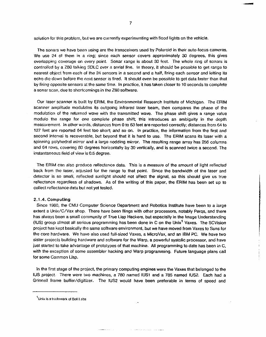
The sonars we have been using are the transceivers used by Polaroid in their auto-focus cameras. We use 24 of them in a ring; since each sensor covers approximately 30 degrees, this gives overlapping coverage on every point. Sonar range is about 30 feet. The whole ring of sonars is controlled by a 280 talking SDLC over a serial line. In theory, it should be possible to get range to nearest object from each of the 24 sensors in a second and a half, firing each sensor and letting its echo die down before the next sensor is fired. It should even be possible to get data faster than that by firing opposite sensors at the same time. In practice, it has taken closer to 10 seconds to complete a sonar scan, due to shortcomings in the 280 software.

Our laser scanner is built by ERIM, the Environmental Research Institute of Michigan. The ERlM scanner amplitude modulates its outgoing infrared laser beam, then compares the phase of the modulation of the returned wave with the transmitted wave. The phase shift gives a range value modulo the range for one complete phase shift; this introduces an ambiguity in the depth measurement. In other words, distances from 0 to 63 feet are reported correctly: distances from 64 to 127 feet are reported 64 feet too short; and so on. In practice, the information from the first and second interval is recoverable, but beyond that it is hard to use. The ERlM scans its laser with a spinning polyhedral mirror and a large nodding mirror. The resulting range array has 256 columns and 64 rows, covering 80 degrees horizontally by 30 vertically, and is scanned twice a second. The instantaneous field of view is 0.5 degree.

The ERlM can also produce reflectance data. This is a measuce of the amount of light reflected back from the laser, adjusled for the range to that point. Since the bandwidth of the laser and detector is so small, reflected sunlight should not affect the signal, so this should give us true reflectance regardless of shadows. As of the writing of this paper, the ERlM has been set up to collect reflectance data but not yet tested.

2.1.4. Computing Since 1980, the CMU Computer Science Department and Robotics Institute have been to a large

extent a Unix/C/Vax shop. There have been flings with other processors, notably Perqs, and there has always been a small community of True Lisp Hackers, but especially in the Image Understanding (IUS) group almost all serious programming has been done in C on the Unix' Vaxes. The SCVision project has kept basically the same software environment, but we have moved from Vaxes to Suns for the core hardware. We have also used full-sized Vaxes, a MicroVax, and an IBM PC. We have two sister projects building hardware and software for the Warp, a powerful systolic processor, and have just started to take advantage of prototypes of that machine. All programming to date has been in C, with the exception of some assembler hacking and Warp programming. Future language plans call for some Common Lisp.

In the first stage of the project, the primary computing engines were the Vaxes that belonged to the IUS project. There were two machines, a 780 named IUS1 and a 785 named IUS2. Each had a Grinnell frame buffer/digitizer. The IUS2 would have been preferable in terms of speed and

'Unix is a trademark of Bell Labs

8

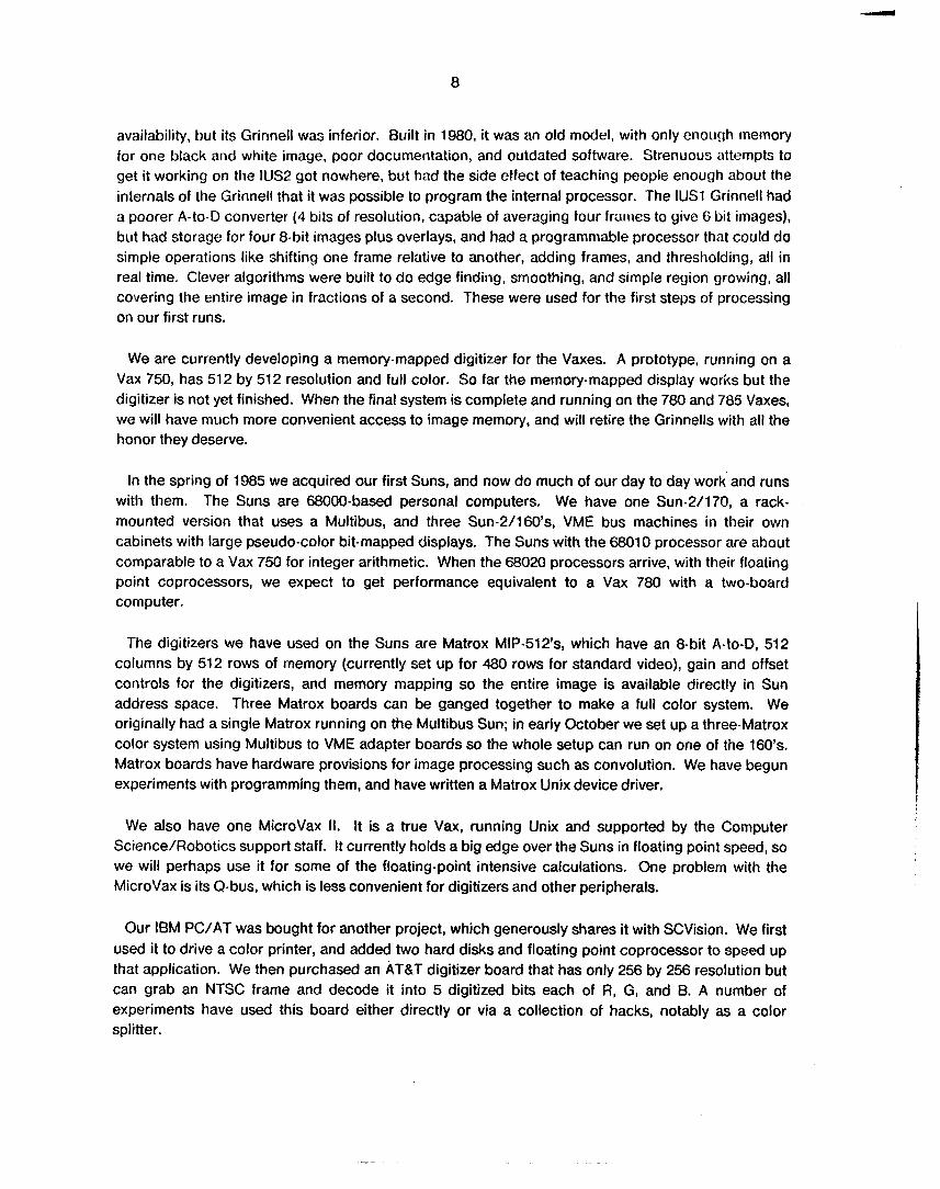
availability, but its Grinnell was inferior. Built in 1980, it was an old model, with only enough memory for one black and white image, poor documentation, and outdated software. Strenuous attempts to get it working on the IUS2 got nowhere, but had the side effect of teaching people enough about the internals of the Grinnell that it was possible to program the internal processor. The IUS1 Grinnell had a poorer A-to-D converter (4 bits of resolution, capable of averaging four frames to give G bit images), but had storage for four 8-bit images plus overlays, and had a programmable processor that could do simple operations like shifting one frame relative to another, adding frames, and thresholding, all in real time. Clever algorithms were built to do edge finding, smoothing, and simple region growing, all covering the entire image in fractions of a second. These were used for the first steps of processing on our first runs.

We are currently developing a memory-mapped digitizer for the Vaxes. A prototype, running on a Vax 750, has 512 by 512 resolution and full color. So far the mernory-mapped display works but the digitizer is not yet finished. When the final system is complete and running on the 780 and 785 Vaxes, we will have much more convenient access to image memory, and will retire the Grinnells with all the honor they deserve.

In the spring of 1985 we acquired our first Suns, and now do much of our day to day work and runs with them. The Suns are 68000-based personal computers. We have one Sun-2/170, a rack- mounted version that uses a Multibus, and three Sun-2/1609s, VME bus machines in their own cabinets with large pseudo-color bit-mapped displays. The Suns with the 68010 processor are about comparable to a Vax 750 for integer arithmetic. When the 68020 processors arrive, with their floating point coprocessors, we expect to get performance equivalent to a Vax 780 with a two-board computer.

The digitizers we have used on the Suns are Matrox MIP-512’s, which have an 8-bit A-to-D, 512 columns by 512 rows of memory (currently set up for 480 rows for standard video), gain and offset controls for the digitizers, and memory mapping so the entire image is available directly in Sun address space. Three Matrox boards can be ganged together to make a full color system. We originally had a single Matrox running on the Multibus Sun; in early October we set up a three-Matrox color system using Multibus to VME adapter boards so the whole setup can run on one of the 160’s. Matrox boards have hardware provisions for image processing such as convolution. We have begun experiments with programming them, and have written a Matrox Unix device driver,

We also have one MicroVax II. It is a true Vax, running Unix and supported by the Computer Science/Robotics support staff. It currently holds a big edge over the Suns in floating point speed, so we will perhaps use it for some of the floating-point intensive calculations. One problem with the MicroVax is its Q-bus, which is less convenient for digitizers and other peripherals.

Our IBM PC/AT was bought for another project, which generously shares it with SCVision. We first used it to drive a color printer, and added two hard disks and floating point coprocessor to speed up that application. We then purchased an AT&T digitizer board that has only 256 by 256 resolution but can grab an NTSC frame and decode it into 5 digitized bits each of R, GI and B. A number of experiments have used this board either directly or via a collection of hacks, notably as a color splitter.

9

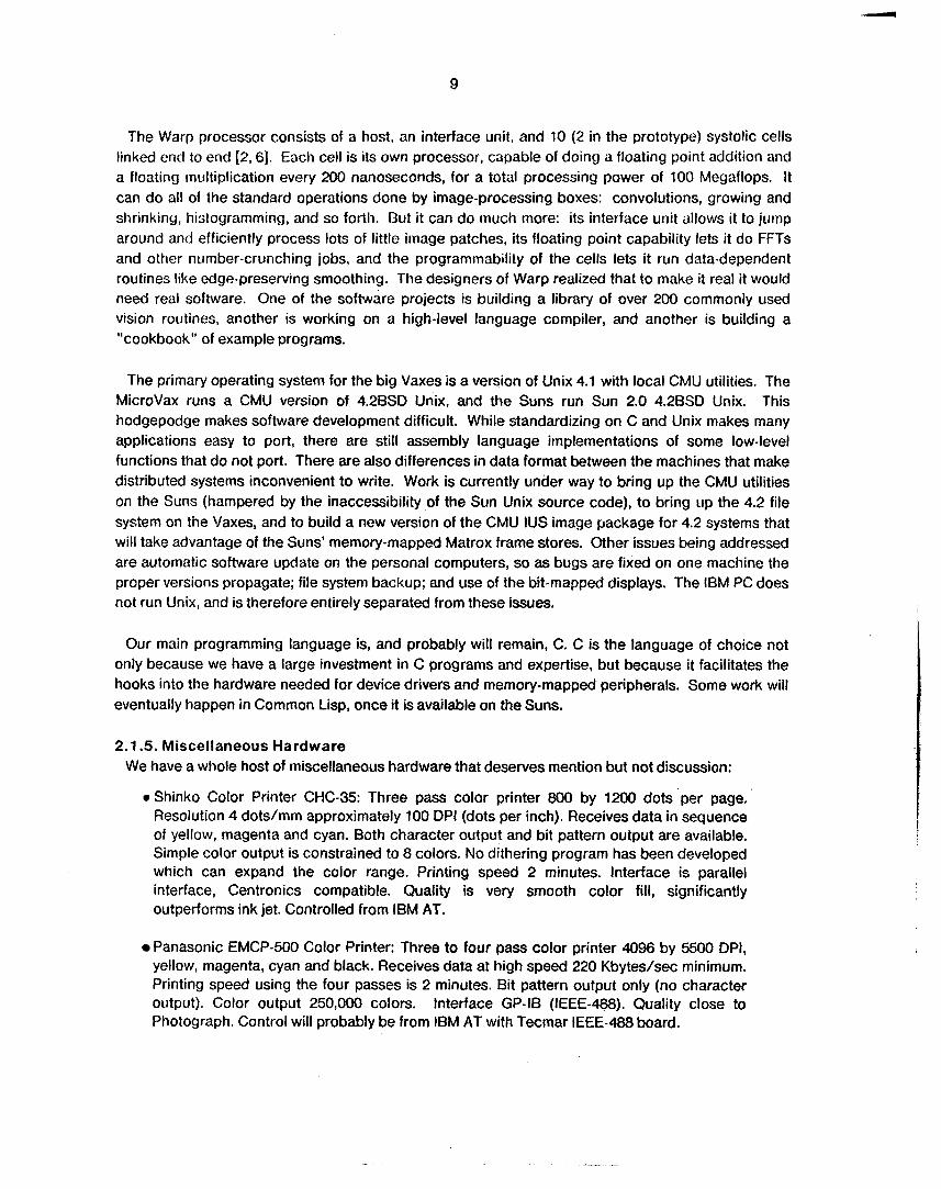
The Warp processor consists of a host. an interface unit. and 10 (2 in the prototype) systolic cells linked end to end [2,6]. Each cell is its own processor, capable of doing a floating point addition and a floating multiplication every 200 nanoseconds, for a total processing power of 100 Megaflops. It can do ell of the standard operations done by image-processing boxes: convolutions, growing and shrinking, hislogramming, and so forth. But it can do much more: its interface unit allows it to juirip around and efficiently process lots of little image patches, its floating point capability lets it do FFTs and other number-crunching jobs, and the programmability of the cells lets it run data-dependent routines like cdge-preserving smoothing. The designers of Warp realized that to make it real it would need real software. One of the software projects is building a library of over 200 commonly used vision routines, another is working on a high-level language compiler, and another is building a “cookbook” of example programs.

The primary operating system for the big Vaxes is a version of Unix 4.1 with local CMU utilities. The MicroVax runs a CMU version of 4.2BSD Unix, and the Suns run Sun 2.0 4.2BSD Unix. This hodgepodge makes software development difficult. While standardizing on C and Unix makes many applications easy to port, there are still assembly language implementations of some low-level functions that do not port. There are also differences in data format between the machines that make distributed systems inconvenient to write. Work is currently under way to bring up the CMU utilities on the Suns (hampered by the inaccessibility of the Sun Unix source code), to bring up the 4.2 file system on the \/axes, and to build a new version of the CMU IUS image package for 4.2 systems that will take advantage of the Suns’ memory-mapped Matrox frame stores. Other issues being addressed are automatic software update on the personal computers, so as bugs are fixed on one machine the proper versions propagate; file system backup; and use of the bit-mapped displays. The IBM PC does not run Unix, and is therefore entirely separated from these issues.

Our main programming language is, and probably will remain, C. C is the language of choice not only because we have a large investment in C programs and expertise, but because it facilitates the hooks into the hardware needed for device drivers and memory-mapped peripherals. Some work will eventually happen in Common Lisp, once it is available on the Suns.

2.1.5. Miscellaneous Hardware We have a whole host of miscellaneous hardware that deserves mention but not discussion:

0 Shinko Color Printer CHC-35: Three pass color printer 800 by 1200 dots per page. Resolution 4 dotslmm approximately 100 DPI (dots per inch). Receives data in sequence of yellow, magenta and cyan. Both character output and bit pattern output are available. Simple color output is constrained to 8 colors. No dithering program has been developed which can expand the color range. Printing speed 2 minutes. Interface is parallel interface, Centronics compatible. Quality is very smooth color fill, significantly outperforms ink jet. Controlled from ISM AT.

Panasonic EMCP-500 Color Printer: Three to four pass color printer 4096 by 5500 DPI, yellow, magenta, cyan and black. Receives data at high speed 220 Kbyteslsec minimum. Printing speed using the four passes is 2 minutes. Bit pattern output only (no character output). Color output 250,000 colors. Interface GP-IS (IEEE-488). Quality close to Photograph. Control will probably be from IBM AT with Tecmar IEEE-488 board.

10

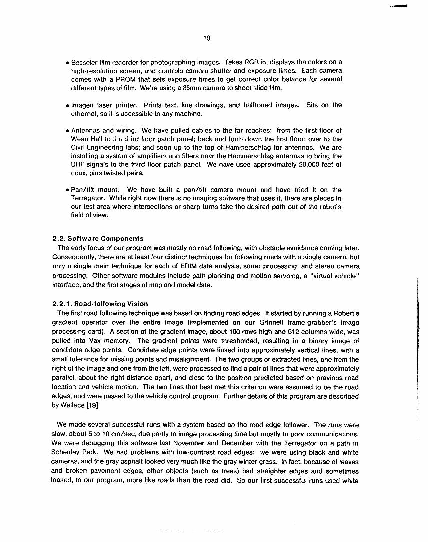
0 Besseler film recorder for photographing images. Takes RGB in, displays the colors on a hiyh-resolution screen, and controls camera shutter and exposure times. Each camera comes with a PROM that sets exposure times to get correct color balance for several different types of film. We're using a 35mm camera to shoot slide film.

0 lmagen laser printer. Prints text, line drawings, and halftoned images. Sits on the ethernet, so it is accessible to any machine.

0 Antennas and wiring. We have pulled cables to the far reaches: from the first floor of Wean Hall to the third floor patch panel: back and forth down the first floor; over to the Civil Engineering labs; and soon up to the top of Hammerschlag for antennas. We are installing a system of amplifiers and filters near the Hammerschlag antennas to bring the UHF signals to the third floor patch panel. We have used approximately 20,000 feet of coax, plus twisted pairs.

0 Pan/tilt mount. We have built a panltilt camera mount and have tried it on the Terregator. While right now there is no imaging software that uses it, there are places in our test area where intersections or sharp turns take the desired path out of the robot's field of view.

2.2. Software Components The early focus of our program was mostly on road following, with obstacle avoidance coming later.

Consequently, there are at least four distinct techniques for following roads with a single camera, but only a single main technique for each of €RIM data analysis, sonar processing, and stereo camera processing. Other software niodules include path plan'ning and motion servoing, a "virtual vehicle" interface, and the first stages of map and model data.

2.2.1. Road-following Vision The first road following technique was based on finding road edges. It started by running a Robert's

gradient operator over the entire image (implemented on our Grinnell frame-grabber's image processing card). A section of the gradient image, about 100 rows high and 512 columns wide, was pulled into Vax memory. The gradient points were thresholded, resulting in a binary image of candidate edge points. Candidate edge points were linked into approximately vertical lines, with a small tolerance for missing points and misalignment. The two groups of extracted lines, one from the right of the image and one from the left, were processed to find a pair of lines that were approximately parallel, about the right distance apart, and close to the position predicted based on previous road location and vehicle motion. The two lines that best met this criterion were assumed to be the road edges, and were passed to the vehicle control program. Further details of this program are described by Wallace [19].

We made several successful runs with a system based on the road edge follower. The runs were slow, about 5 to 10 cm/sec, due partly to image processing time but mostly to poor communications. We were debugging this software last November and December with the Terregator on a path in Schenley Park. We had problems with low-contrast road edges: we were using black and white cameras, and the gray asphalt looked very much like the gray winter grass. In fact, because of leaves and broken pavement edges, other objects (such as trees) had straighter edges and sometimes looked, to our program, more like roads than the road did. So our first successful runs used white

11

masking tape to give reliable road edges. Far later runs, we moved on campus, where the green grass and white cement sidewalks provided much higher contrast, and where the tape was unnecessary.

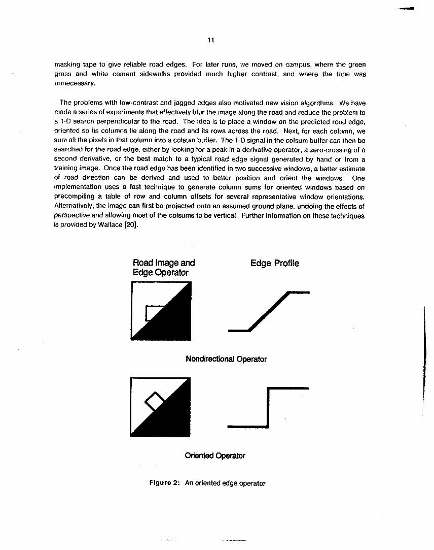
The problems with low-contrast and jagged edges also motivated new vision algorithms. We have made a series of experiments that effectively blur the image along the road and reduce the problem to a 1-D search perpendicular to the road. The idea is to place a window on the predicted road edge, oriented so its columns lie along the road and its rows across the road. Next, for each column, we sum all the pixels in that column into a colsutn buffer. The 1-D signal in the colsum buffer can then be searched for the road edge, either by looking for a peak in a derivative operator, a zero-crossing of a second derivative, or the best match to a typical road edge signal generated by hand or from a training image. Once the road edge has been identified in two successive windows, a better estimate of road direction can be derived and used to better position and orient the windows. One implementation uses a fast technique to generate column sums for oriented windows based on precompiling a table of row and column offsets for several representative window orientations. Alternatively, the image can first be projected onto an assumed ground plane, undoing the effects of perspective and allowing most of the colsums to be vertical. Further information on these techniques is provided by Wallace [20].

Road Image and Edge Operator

Edge Profile

Nondirectional Operator

Oriented Operator

Figure 2: An oriented edge operator

12

i

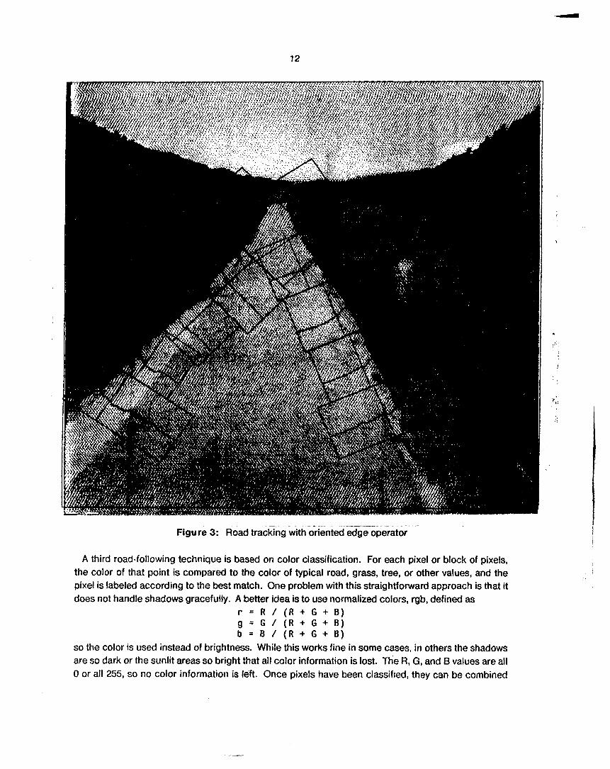
__ -. - - - - - - Figure 3: Road tracking with oriented edge operator

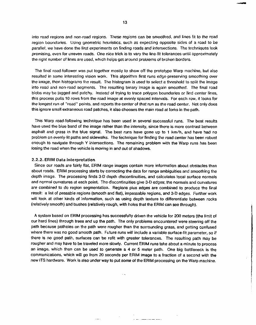
A third road-following technique is based on color classification. For each pixel or block of pixels, the color of that point is compared to the color of typical road, grass, tree, or other values, and the pixel is labeled according to the best match. One problem with this straightforward approach is that it does not handle shadows gracefully. A better idea is to use normalized colors, rgb, defined as

r = R / ( R + G + B) g = G / ( R + G + B) b = B / ( R + G + B )

so the color is used instead of brightness. While this works fine in some cases, in others the shadows are so dark or the sunlit areas so bright that all color information is lost. The R, G, and B values are all 0 or all 255, so no color information is Ie'ft. Once pixels have been classified, they can be combined

13

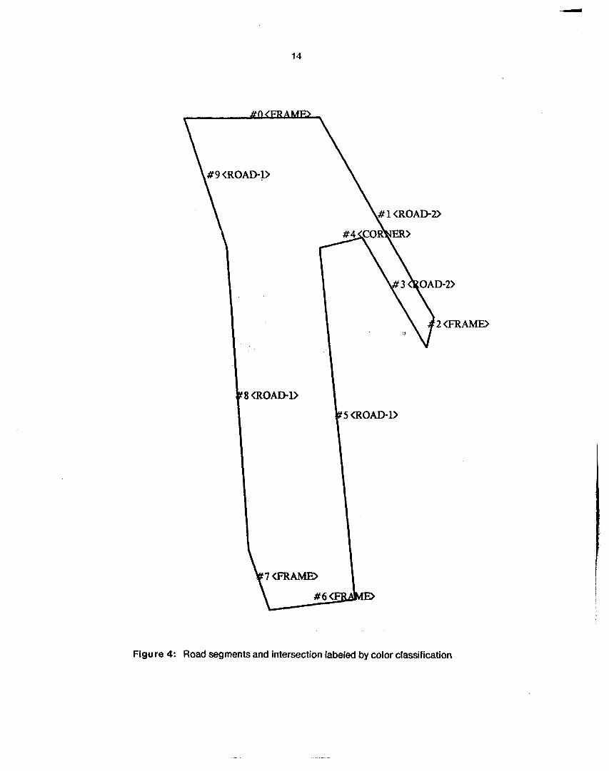
into road regions and non-road regions. These regions can be smoothed, and lines fit to the rood region boundaries. Using geometric heuristics, such as expecting opposite sides of a road to be parallel, we have done the first experiments on finding roads and intersections. The techniques look promising, even for uneven roads. One nice trick is to vary the line-fit tolerances until approximately the right number of lines are used, which helps get around problems of broken borders.

The final road-follower was put together mostly to show off the prototype Warp machine, but also resulted in some interesting vision work. This algorithm first runs edge-preserving smoothing over the image, then histograms the result. The histogram is used to select a threshold to split the image into road and non-road segments. The resulting binary image is again smoothed. The final road blobs may be jagged and patchy. Instead of trying to trace polygon boundaries or find center lines, this process pulls 10 rows from the road image at evenly spaced intervals. For each row, it looks for the longest run of "road" points, and reports the center of that run as the road center. Not only does this ignore small extraneous road patches, it also chooses the main road at forks in the path.

This Warp road-following technique has been used in several successful runs. The best results have used the blue band of the image rather than the intensity, since there is more contrast between asphalt and grass in the blue signal. The best runs have gone up to 1 km/h, and have had no pioblem on evenly-lit paths and sidewalks. The technique for finding the road center has been robust enough to navigate through Y intersections. The remaining problem with the Warp runs has been losing the road when the vehicle is moving in and out of shadows.

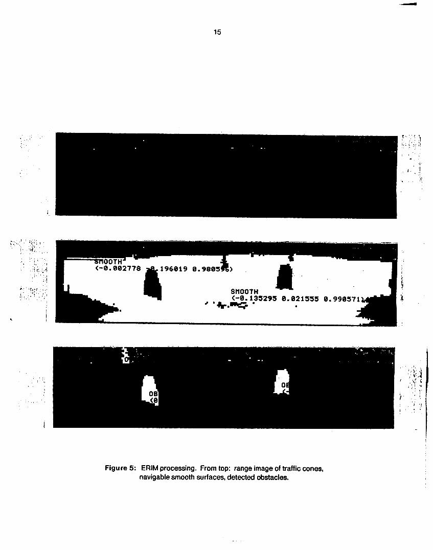
2.2.2. ERlM Data Interpretation Since our roads are fairly flat, ERlM range images contain more information about obstacles than

about roads. ERlM processing starts by correcting the data for range ambiguities and smoothing the depth image. The processing finds 3-D depth discontinuities, and calculates local surface normals and normal curvatures at each point. The discontinuities give 3-0 edges; the normals and curvatures are combined to do region segmentation. Regions plus edges are combined to produce the final result: a list of passable regions (smooth and flat), impassable regions, and 3-D edges. Further work will look at other kinds of information, such as using depth texture to differentiate between rocks (relatively smooth) and bushes (relatively rough, with holes that the ERIM can see through).

A system based on ERlM processing has successfully driven the vehicle for 200 meters (the limit of our hard lines) through trees and up the path. The only problems encountered were steering off the path because potholes on the path were rougher than the surrounding grass, and getting confused where there was no good smooth path. Future runs will include a variable surface-fit parameter, so i f there is no good path, surfaces can be refit with greater tolerances. The resulting path may be rougher and may have to be traveled more slowly. Current ERlM runs take about a minute to process an image, which then can be used to generate a 4 or 5 meter path. One big bottleneck is the communications, which will go from 20 seconds per ERlM image to a fraction of a second with the new ITS hardware. Work is also under way to put some of the ERlM processing on the Warp machine.

14

. A M D

Figure 4: Road segments and intersection labeled by color classification

15

Figure 5: ERlM processing. From top: range image of traffic cones, navigable smooth surfaces, detected obstacles.

16

2.2.3. Sonar Processing The difficulty in sonar processing is to take relatively crude data, 24 range measurements, each

reporting the distance to the nearest object in a 30 degree cone, and produce relatively high- resolution output. The saving factor is the overlap between cones of coverage of neighboring sensors on a single scan, and of multiple sensors as the vehicle moves. A range measurerrient not only says that there is some object at the indicated range: it also says that there is no other object closer than that range in that 30 degree cone. The source of the echo can be represented as a probability smear along the arc at the end of the cone. If some overlapping scan shows that part of that arc must be empty, the "probabilities" on that part of the arc can be reduced, and the weights on the rest of the arc increased. By the time several scans are combined in this way, the data can be represented on a grid with as little as 1 cm resolution, although 10 or 20 cm resolution usually gives a better tradeoff between computation, storage, and accuracy. Each point on the grid contains a "probability" that that point is empty, and a "probability" that it is occupied. Because of double echoes and other sensor imperfections, the "probabilities" don't necessarily add up to 1; hence the quotes. The residual is a measure of the uncertainty of the information in that point. Post-processing stages can threshold the occupied weights and return a list of polygonal obstacles. Other recent additions to the program are a process that continually adds new data to the grid without having to reanalyze the old scans, and a method of keeping the local map centered on the current vehicle location [l].

Our best sonar runs have maneuvered the Terregator through the trees on Flagstaff Hill. Even with the Terregator slipping on the grass and with unreliable sensors, the redundancy in the data and processing is enough to build a robust system. Sonar runs now take about 30 seconds per step, with each step about two meters. Actual computation time is less than 5 seconds. When the sonar hardware is improved, we should be able to do continuous motion.

2.2.4. Stereo Vision The FlDO system finds three dimensional obstacles in a stereo pair of images [18]. To correctly

interpret the stereo pair, FlDO must match points in left image with the corresponding points in the right image. First, points in the right image are selected. The points chosen are corners and isolated spots that should be easy to locate in the left image. In the next step, FlDO finds the approximate position of each chosen point in a low-resolution version of the left image. The position estimate is improved by finding the point in higher and higher resolution images. Once the point has been exactly located in the left image, triangulation gives the location of that point in three dimensions. By matching the same points in several image pairs over time, we can get more accurate point position estimates and can derive the vehicle's motion. We now have versions of FlDO that run on the Vax and on the Suns, and are porting it to the Warp machine. Details of FIDOs predecessor are given by Moravec [8].

FlDO has made many successful runs, mostly indoors with Neptune. We made one good outdoor Neptune run, with an umbrella taped to the camera mast to keep the robot dry during a rain shower. Our outdoor FlDO runs on the Terregator have the same problems that have plagued other outdoor vision runs: shadows, sun, and insufficient dynamic range on the cameras. FlOO currently takes about a minute per step on either a Vax or a Sun. Warp FlDO will run in about 3 seconds per step, fast enough for reasonable continuous motion.

17

... . * . . . . m . . . . . . . . . . . . . . . . . . . . . . . . . . . . . . . . . . . . * . . . . . . . . . . . . . . . . . . . . . . . . . . . . . . . ... . . . ... . . . . . . . . . . . . . . . . . . . . . . . . ... . . . . . . . . . . . .

. ' " . . . . . . . . . . . . . . . . . . . . . . X . . * ......................................... . . " . . . . . . . . . . . . . . . . . . . . X X + + + . . . . . . . . . . . . . . . . . . . . . . . . . . . . . . . . . . . . . . . . . .

. . . . . . . . . , . . . . . . . . . . . . . r****+. . . . . . . . . . . .~. . . . . . . . . . . . . . . . . . . ,* . . . . . . . . . . . . . . . . . . . . . . . . . . . . . . . . . . . . . .+++++.. . . . . . . . . . . . . . . . . . . . . . . . . . . . . . . . . . . . . . . . .

t + + t

. . . . . . . . . . . . . . . . . . . . . . . . . . . . . . ................................................................... ................................................................... ....................................................................

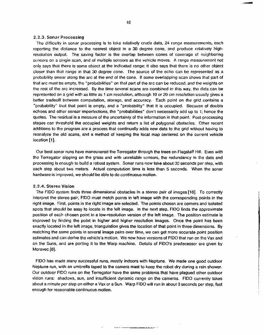
. . . . . . . . . . . . .... . . . . . . . . . . . . . . . . . . . . . . . . . . . . . . . . . . . . . . . . . . . . . . . . . . . . . . . . . . . . .... . . . . . . . . . . . . . . . . . . . . . . . . . . . . . . . . .... . . . . . . . . . . . . .... .... . . . . . . . . .... . . . . Figure 6: A two-dimensional sonar map. Emply areas with a high certainty

factor are represented by white areas; lower certainty factors by 'I + 'I symbols of increasing thickness. Occupied areas are represented by "XI' symbols, and Unknown areas by " - " .

The position of the robot is shown by a circle and the outline of the room and of the major objects by a solid line.

2.2.5. Motion Once the road and obstacles have been found, we have to plan a path that avoids obstacles and

move the vehicle along that path. We have developed several methods, partly to try various ideas and partly to have specialized algorithms that are better tuned for certain conditions.

In FlDO we developed path relaxation, a path planning algorithm that finds the lowest "cost" path from the current position to the goal. The cost of traversing a particular point can be a combination of several factors, including distance traveled, nearness' to objects, traversability of the terrain, and uncertainty about the area. The first step of path relaxation finds a preliminary path on an eight- connected grid of points. The second step adjusts, or "relaxes," the position of each preliminary path point to improve the path. We have used path relaxation for ERIM, sonar, and stereo vision runs. Obstacles are given a high cost, areas outside the field of view or hidden behind obstacles a medium cost, and known empty areas a low cost. Path Relaxation is documented by Thorpe [17, 181.

The output of path relaxation is a list of points through which the planned path passes. These

points can be directly used by a simple-minded scheme that drives the vehicle through each point in turn. A better strategy is to use the points as "critical points" in a scheme that plans local trajectories based on critical points, vehicle dynamics, and local obstacles. One such local controller, built as part of a separate project at CMU, is Dynamic Obstacle Avoidance Control (OAC). The OAC algorithm builds a "potential field," where obstacles repel the vehicle and the critical points attract the vehicle along the path. What makes this approach unique is that the strength of the repulsive forces varies with the closing speed of the vehicle and the obstacle. Thus, for instance, i f the vehicle has to squeeze through a narrow space, it will slow down as it approaches, then resume its speed as it passes through. The combination of algorithms makes for a good division of the problem: path relaxation takes care of global issues, such as avoiding dead ends, finding an overall optimal or near-optimal path, and deciding between areas with different terrain or better visibility. Local issues, such as cutting corners, slowing the vehicle to maneuver in tight spots, and smooth transitions from one step to the next, are all handled by the lower-level controller. The low-level controller can also react to new sensory data as the vehicle moves, and can often handle new objects or updated obstacle positions without having to invoke the global path planner [41 51.

We have a specialized controller for following obstacle-free roads. The genesis of this controller was our early work in visual servoing, Previous ideas for control often steered too sharply or not sharply enough, letting one of the edges of the road drift out of our field of view and fouling up the image processing. The easiest solution is to servo so that the road always stays in the picture: essentially, lining up a "hood ornament" with the center line. Moreover, the analysis of this strategy is tractable, and there is a closed form solution for critically darriped gain. Even if the gain is off by large factors, the system still behaves relatively well. In some of our Warp runs the camera wasn't even calibrated; the gain parameters were estimated and tweaked until the system worked, with no precise measurements. In the control literature this method is called "pure pursuit."

2.2.6. Virtual Vehicle To simplify development of subsequent versions of vehicles, we are developing a virtual vehicle

interface. The motivation behind isolating a set of generic commands is that high level "conceptual" development need not be concerned about implementation details, and changes made to the hardware (motors, sensors, etc) are invisible to the higher level software. The only changes that need to be made are to the drivers that control the sensors and motors (a relatively simpler task).

There are two parts to the virtual vehicle: motion control and sensor data acquisition. The sensor part of the interface is still in the design phase. It will be responsible for getting a reading (image, range image, sonar scan, etc.), storing it in some known spot, and time-stamping the data.

The virtual vehicle motion interface will, for now, be limited to following arcs and lines supplied to it by a host computer. The communication between host and virtual vehicle falls under the following categories:

0Set commands: acceleration.

Commands specified by host to set parameters like speed and

- - 0 Query Commands: Queries by the host about status of devices, position of vehicle, etc.

0 Report Commands: Reports initiated by the virtual vehicle concerning alarm situations.

19

All communication will have two checks. First, each packet will be prefixed with the length of the string. Upon receiving the packet, the listening device will check to see if m y data is lost in the transmission. Second, data that constitutes crucial commands is further checked to see if the arguments specified are within acceptable range before the command is executed. In both cases, the listening device validates the data and sends either ACK (acknowledge) or NAK (error in data received) to the sender. The sender is responsible for ensuring that it gets an.acknowledgment for the data sent. I f either a NAK or no signal is received, then the sender repeats the old transmission until a limit is reached or an ACK is received.

Normal interaction between host and virtual vehicle is envisioned as follows:

0 Host issues an arc length and steering angle.

0 Virtual vehicle completes the current arc and then embarks upon the new arc. Transition to a new arc initiates a new steering angle.

0 When the vehicle has traveled the arc length specified, a signal is issued to the host along with time and x,y position of the vehicle.

This position is used to predict the next arc (and corresponding steering angle) which is sent to the virtual vehicle.

It is neither possible nor desirable for the virtual vehicle level to be completely vehicle-independent. It may be important, for instance, for path-planning to know if a vehicle can turn in place. l h e details that should be masked, however, are those of a particular vehicle’s commands to make it perform one if its maneuvers, and the lowest-level commands of how to get a sensor reading and how to correct it for vehicle motion. Such an interface allows us to change the low-level steering and moving commands of a vehicle without redesigning the rest of the system.

2.2.7. Data Some of the most interesting issues on this project are the interactions of the perceived world with

predictions. A prediction module will take current vehicle position, look up in the map to determine what should be out there, and generate predicted appearances and geometries of terrain and objects. We are just in the first stages of building those maps and models. The most extensive maps are being generated by the U.S. Army Engineer Topographic Labs to cover the entire 2 km by 2 km Martin Marietta ALV test site. The map will consist of

0 Elevation grid, every 5 meters, with resolution to a fraction of a meter and accuriicy to about 2 meters.

0 Overlay for hydrology. The aerial photointerpreters can find any gully deeper than 1 foot and wider than 2 feet.

0 Overlay for ground cover. Trees, low grass, brush, etc.

0 Overlay for soil type. Sand, loam, clay, mixed rocks, etc.

Overlay for slopes. Polygons with average slope for each.

20

e Overlay for cultural features. including roads, fences, power lines, and buildings.

2.3. Architecture The proliferation of modules could rapidly lead to pandemonium unless some order is imposed on

the system architecture. This is not a straightforward task: system configuration is one of the research topics, and interacts strongly with what modules are available and how they perform. We have built several specialized systems, basically one for each sensor interpretation program, and now have enough experience to start tying things together in a more organized fashion.

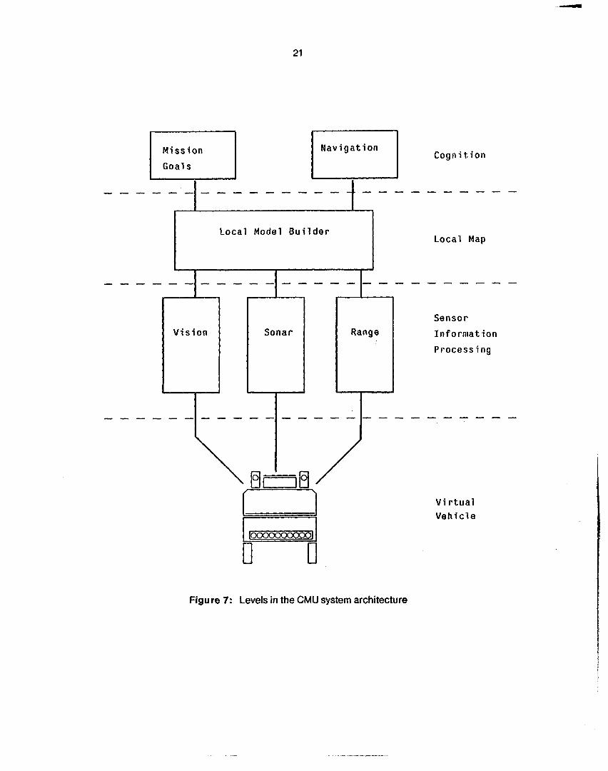
Our new architecture contains the physical hardware plus four main software levels: a virtual vehicle interface for motion and sensing, sensor and motion processing, the local map level, and high-level cognition (figure 7). While there are no hard and fast boundaries between these levels, they provide both a conceptual way of breaking down the system and a model for where the main channels of information flow should be.

The hardware consists of the Navlab, if funded, plus stereo color cameras, the ERlM scanner, sonars, and pan/tilt mounts. The virtual vehicle level is a set.of functions that mask the particular details of how the vehicle moves and senses. Most of our existing sensor interpretation processes can be converted into the format needed for the new architecture. These processes start with raw data and produce descriptions in three-dimensional world coordinates. The interface to the sensors is handled by the virtual vehicle, so that arriving data has been time-tagged and possibly corrected for vehicle motion. From the raw data, each sensor process produces viewpoint- and sensor-dependent symbolic descriptions. The sensor modules for the system include image, sonar, range, and vehicle motion routines.

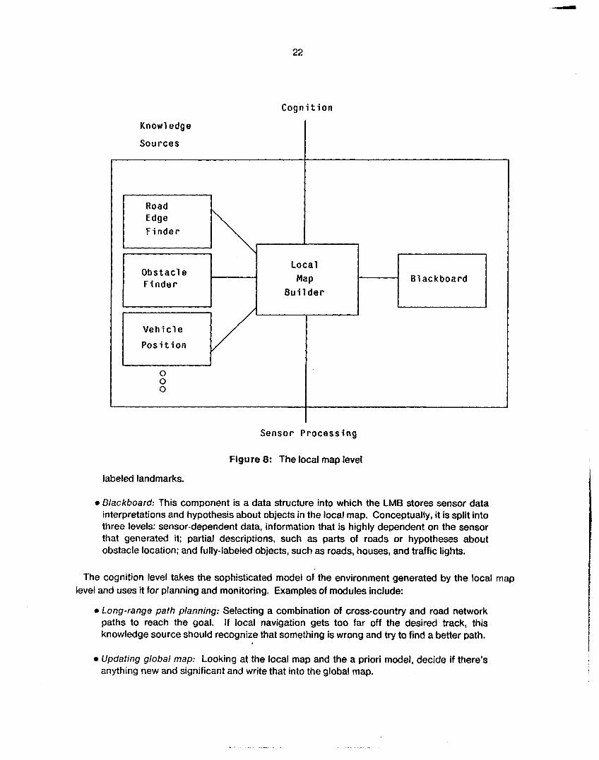
The local map level is responsible for building and maintaining a description of the environment around the vehicle. It begins with data from the sensor interpretation processes which has no semantic labels. By the time the map is ready for the cognition level, it must be sensor-independent and labeled (for example, "road," "landmark," or "house"). The components of the local map level are the local map builder that orchestrates the processing, knowledge sources that do the work, and the blackboard that stores the data (figure 8):

.Local map builder (LMS:) This component controls the local map. The LMB is responsible for taking requests from navigation and goal-seeking modules, listening to data from the sensor interpretation processes, and then selecting knowledge sources to run. This gives the LMB a dual role, as both an interface and data channel, and as a scheduler for the knowledge sources.

0 Knowledge sources (KS:) This component consists of expert or specialized modules that retrieve partial descriptions from the local map, generate higher-level descriptions, and write back into the local map. Possible KS modules include a road finder, which takes vision lines, range lines, vision and range surfaces, and previous road position and decides where the most likely road position is; an obstacle finder, which examines the current planned path, sonar blobs, and range blobs and produces a list of obstacles; a vehicle position estimator, which takes motion output and matches sensed features against predicted map features to produce the best vehicle position: and a landmark identifier, which takes 3-D surfaces and lines, examines the global map, and produces

21

Miss ion

Goals

I

I

Sonar

-T-

Range

Cogt i i t ion

- - - - -

Local Map

Sensor

I n f o m a t i o n

Processing

- - - - -

V i r t u a l V e h i c l e

Figure 7: Levels in the CMU system architecture

22

Local

Map Bui 1 der

Obstacle Finder

Cognit ion

Know1 edge

Sources

I Blackboard

I 1 I

I C

Veh i c l e

Pos i t i on

0 0 0

I

I Sensor Processing

Figure 8: The local map level

labeled landmarks.

0 Blackboard: This component is a data structure into which the LMB stores sensor data interpretations and hypothesis about objects in the local map. Conceptually, it is split into three levels: sensor-dependent data, information that is highly dependent on the sensor that generated it; partial descriptions, such as parts of roads or hypotheses about obstacle location; and fully-labeled objects, such as roads, houses, and traffic lights.

The cognition level takes the sophisticated model OF the environment generated by the local map level and uses it for planning and monitoring. Examples of modules include:

e Long-range path planning: Selecting a combination of cross-country and road network paths to reach the goal. If local navigation gets too far off the desired track, this knowledge source should recognize that something is wrong and try to find a better path.

e Updating global map: Looking at the local map and the a priori model, decide if there’s anything new and significant and write that into the global map.

23

Landmark recognition strategizer: Deciding when the dead-reckoned position has drifted too much and it is necessary to recalibrate. Picks a set of landmarks and a strategy for being able to see them, and tasks the lower level with finding and recognizing enough of them to get a good positioned fix.

2.4. Blackboard The underlying mechanism on which the local map level is implemented is a blackboard. The

blackboard is a database of tokens, data objects consisting of a set of attribute-value pairs determined by the token’s type. The Local Map Builder (LMB) is the blackboard’s traffic manager. It services requests from knowledge source, sensor, and cognition modules to store and retrieve tokens from the blackboard. The LMB is equipped with a pattern-matching mechanism for specifying which tokens to recover. Additional tasks performed by the LMB include scheduling token requests, expiring old and uninteresting tokens, and transforming spatial data from one coordinate frame to another. The LMB is implemented as an independent module, separately compiled, running as a stand-alone process complete with network and inter-process communication channels and primitives for communicating with other processes. The blackboard is implemented as a collection of data structures residing in the address space of the LMB.

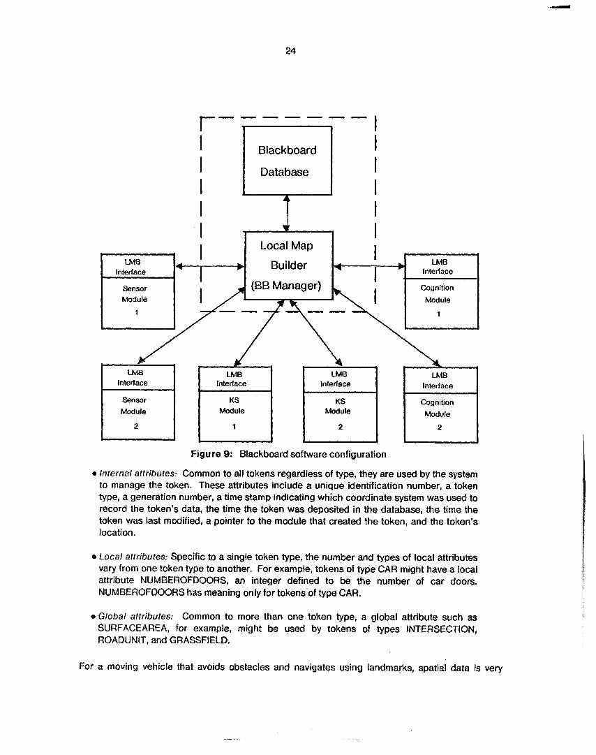
The blackboard software package provides the user with a library of C data structures and functions necessary for writing sensor, KS, and cognition modules for use in the blackboard system (see figure 9). More specifically, the package provides the following facilities:

e Token manipulation: mechanisms for declaring, allocating, deleting, reading, and writing composite data objects (tokens) residing in the user’s address space. Each token consists of a list of attribute-value pairs.

e Coordinate frame manipulation: mechanisms for defining, changing, transforming, and deleting coordinate frames in which the world, vehicle, sensors, and physical objects are expressed.

e Geometric reasoning: functions provided to calculate distances between objects (polygons, lines, point clusters, etc.), calculate convex hulls, determine orientations, and do other common geometric reasoning.

e Specification manipulation: mechanisms for building patterns used for matching and recovering tokens residing in the blackboard database. Each pattern is a boolean expression of functions and relations defined over data attributes. A token matches a pattern i f its attributes satisfy the boolean expression.

e Blackboard Communication: mechanisms for depositing tokens into the blackboard database and for retrieving them, either by pattern-matching specification or direct token addressing .

A token is a data unit capable of representing an object of any type (such as a road, an intersection, an obstacle, or a landmark) or instructions or status information to be passed between modules. Each token is composite, consisting of a set of attribute-value pairs. An attribute value is a system defined type or a primitive type, used to characterize a token. Attributes fall into three categories:

.

24

1 I

Cognition

Module --

Module

Figure 9: Blackboard software configuration

0 Internal attributes: Common to all tokens regardless of type, they are used by the system to manage the token. These attributes include a unique identification number, a token type, a generation number, a time stamp indicating which coordinate system was used to record the token’s data, the time the token was deposited in the database, the time the token was last modified, a pointer to the module that created the token, and the token’s location.

0 Local attributes: Specific to a single token type, the number and types of local attributes vary from one token type to another. For example, tokens of type CAR might have a local attribute NUMBEROFDOORS, an integer defined to be the number of car doors. NUMBEROFDOORS has meaning only for tokens of type CAR.

0 Global attributes: Common to more than one token type, a global attribute such as SURFACEAREA, for example, might be used by tokens of types INTERSECTION, ROADUNIT, and GRASSFIELD.

For a moving vehicle that avoids obstacles and navigates using landmarks, spatial data is very

25

important: therefore, all tokens have an internal attribute TLOCATION of type location. A location is a collection of three-dimensional points to describe the shape of an object expressed in some coordinate frame. Depending on the nature of the represented object, one coordinate frame may be more appropriate than another. For example, stationary objects such as landmarks are most suitably expressed in a world coordinate frame, while sensors mounted on the vehicle are best expressed in a vehicle-based frame. The blackboard package contains a powerful set of functions for defining and manipulating locations, coordinate frames, and spatial descriptions.

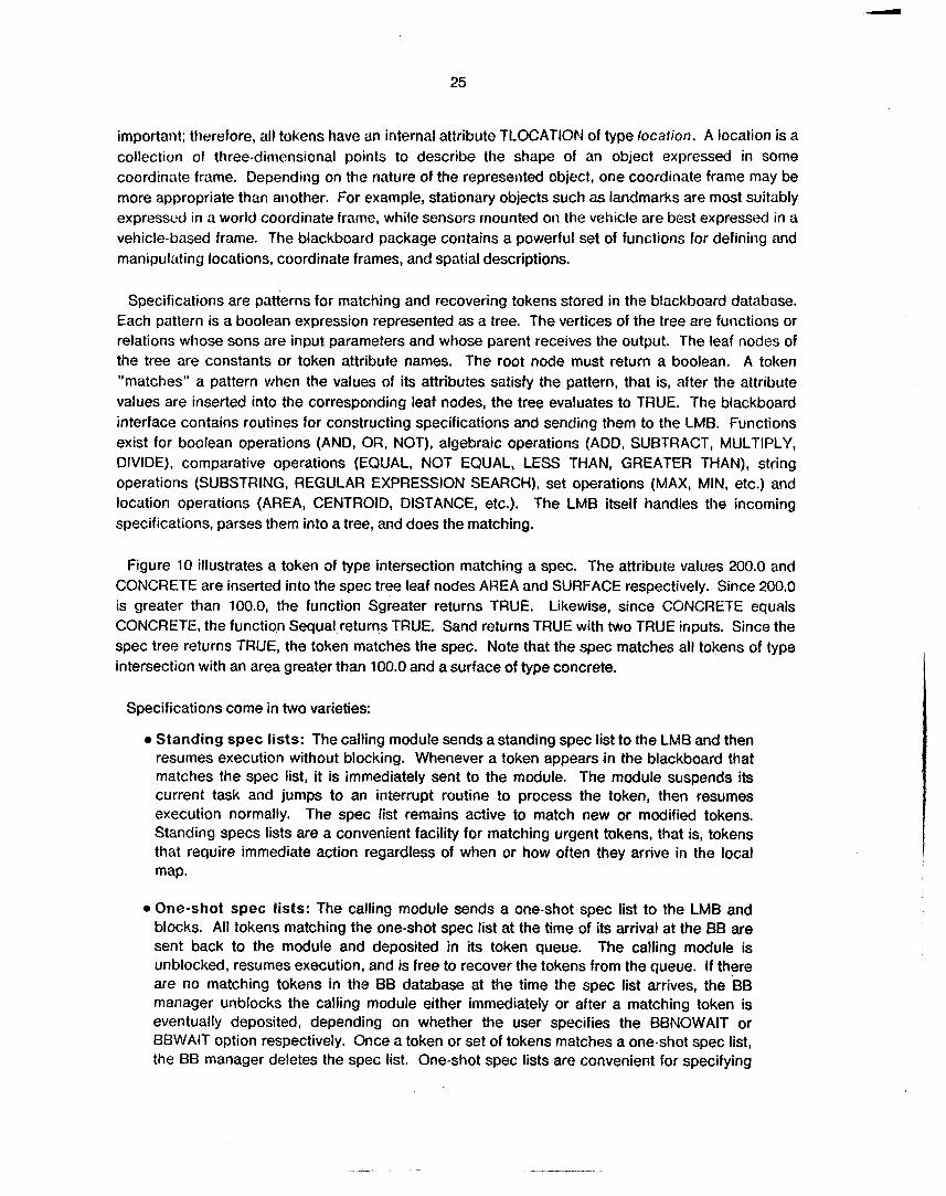
Specifications are patterns for matching and recovering tokens stored in the blackboard database. Each pattern is a boolean expression represented as a tree. The vertices of the tree are functions or relations whose sons are input parameters and whose parent receives the output. The leaf nodes of the tree are constants or token attribute names. The root node must return a boolean. A token "matches" a pattern when the values of its attributes satisfy the pattern, that is, after the attribute values are inserted into the corresponding leaf nodes, the tree evaluates to TRUE. The blackboard interface contains routines for constructing specifications and sending them to the LMB. Functions exist for boolean operations (AND, OR, NOT), algebraic operations (ADO, SUBTRACT, MULTIPLY, DIVIDE), comparative operations (EQUAL, NOT EQUAL, LESS THAN, GREATER THAN), string operations (SUBSTRING, REGULAR EXPRESSION SEARCH), set operations (MAX, MIN, etc.) and location operations (AREA, CENTROID, DISTANCE, etc.). The LMB itself handles the incoming specifications, parses them into a tree, and does the matching.

Figure 10 illustrates a token of type intersection matching a spec. The attribute values 200.0 and CONCRETE are inserted into the spec tree leaf nodes AREA and SURFACE respectively. Since 200.0 is greater than 100.0, the function Sgreater returns TRUE. Likewise, since CONCRETE equals CONCRETE, the function Sequal returns TRUE. Sand returns TRUE with two TRUE inputs. Since the spec tree returns TRUE, the token matches the spec. Note that the spec matches all tokens of type intersection with an area greater than 100.0 and a surface of type concrete.

Specifications come in two varieties:

0 Standing spec lists: The calling module sends a standing spec list to the LMB and then resumes execution without blocking. Whenever a token appears .in the blackboard that matches the spec list, it is immediately sent to the module. The module suspends its current task and jumps to an interrupt routine to process the token, then resumes execution normally. The spec list remains active to match new or modified tokens. Standing specs lists are a convenient facility for matching urgent tokens, that is, tokens that require immediate action regardless of when or how often they arrive in the local map.

0 One-shot spec lists: The calling module sends a one-shot spec list to the LMB and blocks. All tokens matching the one-shot spec list at the time of its arrival at the BB are sent back to the module and deposited in its token queue. The calling module is unblocked, resumes execution, and is free to recover the tokens from the queue. If there are no matching tokens in the BB database at the time the spec list arrives, the 'sf3 manager unblocks the calling module either immediately or after a matching token is eventually deposited, depending on whether the user specifies the BBNOWAIT or BBWAIT option respectively. Once a token or set of tokens matches a one-shot spec list, the BB manager deletes the spec list. One-shot spec lists are convenient for specifying

26

intersect ion

Function

SPEC TREE

CONCRETE Attribute Value

200.0

I I Sand

Function

Sg reater

200.0 CONCRETE CONCRETE

/ Local Attribute ot Intersection

TOKEN

\ floating Point

Constant

/ Global Attribute

Surface

/ \ \

\

/ /

Attribute I Surface I Name 5 I Ttype I Area

Enumerated

CONCRETE

Attribute Value

Figure 1 0: Example of a token matching a spec

what tokens a module needs currently. between calling modules and the 66 manager.

They force tightly-coupled synchronization

Communications between the blackboard and modules is handled by routines provided as part of the blackboard package. Routines are provided to set up communications channels, deposit a token in the blackboard, send a one shot or standing token specification, and so on. Since the routines called by both the modules and the LMB are provided, they can use any protocol they wish. We will have specialized versions optimized for known environments, and generic versions that use IP/TCP that run on a wider variety of hardware.

27

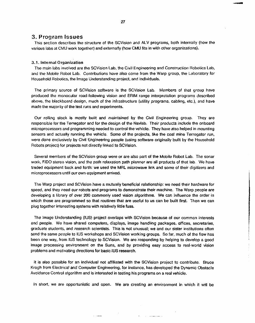
3. Program Issues This section describes the structure of the SCVision and ALV programs, both internally (how the

various labs at CMU work together) and externally (how CMU fits in with other organizations).

3.1. Internal Organization The main labs involved are the SCVision Lab, the Civil Engineering and Construction Robotics Lab,

and the Mobile Robot Lab. Contributions have also come from the Warp group, the Laboratory for Household Robotics, the Image llnderstanding project, and individuals.

The primary source of SCVision software is the SCVision Lab. Members of that group have produced the monocular road-following vision and ERlM range interpretation program described above, the blackboard design, much of the infrastructure (utility programs, cabling, etc.), and have made the majority of the test runs and experiments.

Our rolling stock is mostly built and maintained by the Civil Engineering group. They are responsible for the Terregator and for the design of the Navlab. Their products include the onboard microprocessors and programming needed to control the vehicle. They have also helped in mounting sensors and actually running the vehicle. Some of the projects, like the coal mine Terregator run, were done exclusively by Civil Engineering people (using software originally built by the Household Robots project) for projects not directly linked to SCVision.

Several members of the SCVision group were or are also part of the Mobile Robot Lab. The sonar work, FlDO stereo vision, and ?he path relaxation path planner are all products of that lab. We have traded equipment back and forth: we used the MRL microwave link and some of their digitizers and microprocessors until our own equipment arrived.

The Warp project and SCVision have a mutually beneficial relationship: we need their hardware for speed, and they need our robots and programs to demonstrate their machine. The Warp people are developing a library of over 200 commonly used vision algorithms. We can influence the order in which those are programmed so that routines that are useful to us can be built first. Then we can plug together interesting systems with relatively little fuss.

The Image Understanding (IUS) project overlaps with SCVision because of our common interests and people. We have shared computers, displays, image handling packages, offices, secretaries, graduate students, and research scientists. This is not unusual; we and our sister institutions often send the same people to IUS workshops and SCVision working groups. So far, much of the flow has been one way, from IUS technology to SCVision. We are .responding by helping to develop a good image processing environment on the Suns, and by providing easy access to real-world vision problems and motivating directions for basic IUS research.

It is also possible for an individual not affiliated with the SCVision project to contribute. Bruce Krogh from Electrical and Computer Engineering, for instance, has developed the Dynamic Obstacle Avoidance Control algorithm and is interested in testing his programs on a real vehicle.

In short, we are opportunistic and open. We are creating an environment in which it will be

28

conducive to bring in new ideas, both ours and from other groups. As the robot and its systems become more and more complicated, and as the interactions inside the system becorrie important research topics on their own, it is more difficult and expensive to build a complete system. It therefore becomes more important for us to share and to become an open resource.

3.2. External Organization

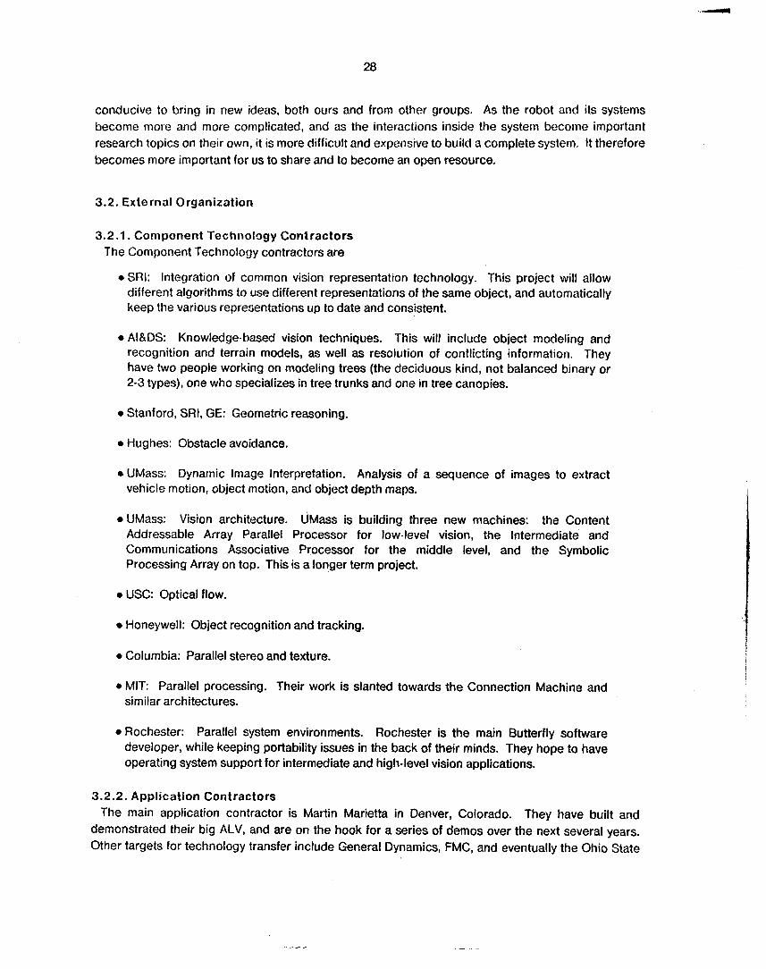
3.2.1. Coniponent Technology Contractors The Component Technology contractors are

0 SRI: Integration of common vision representation technology. This project will allow different algorithms to use different representations of the same object, and automatically keep the various representations up to date and consistent.

0 AI&DS: Knowledge-based vision techniques. This will include object modeling and recognition and terrain models, as well as resolution of conflicting information. They have two people working on modeling trees (the deciduous kind, not balanced binary or 2-3 types), one who specializes in tree trunks and one in tree canopies.

0 Stanford, SRI, GE: Geometric reasoning.

0 Hughes: Obstacle avoidance.

s UMass: Dynamic Image Interpretation. Analysis of a sequence of images to extract vehicle motion, object motion, and object depth maps.

0 UMass: Vision architecture. UMass is building three new machines: the Content Addressable Array Parallel Processor for low-level vision, the Intermediate and Communications Associative Processor for the middle level, and the Symbolic Processing Array on top. This is a longer term project.

0 USC: Optical flow.

0 Honeywell: Object recognition and tracking.

0 Columbia: Parallel stereo and texture.

0 MIT: Parallel processing. Their work is slanted towards the Connection Machine and similar architectures.

0 Rochester: Parallel system environments. Rochester is the main Butterfly software developer, while keeping portability issues in the back of their minds. They hope to have operating system support for intermediate and high-level vision applications.

3.2.2. Application Contractors The main application contractor is Martin Marietta in Denver, Colorado. They have built and

demonstrated their big ALV, and are on the hook for a series of demos over the next several years. Other targets for technology transfer include General Dynamics, FMC, and eventually the Ohio State

29

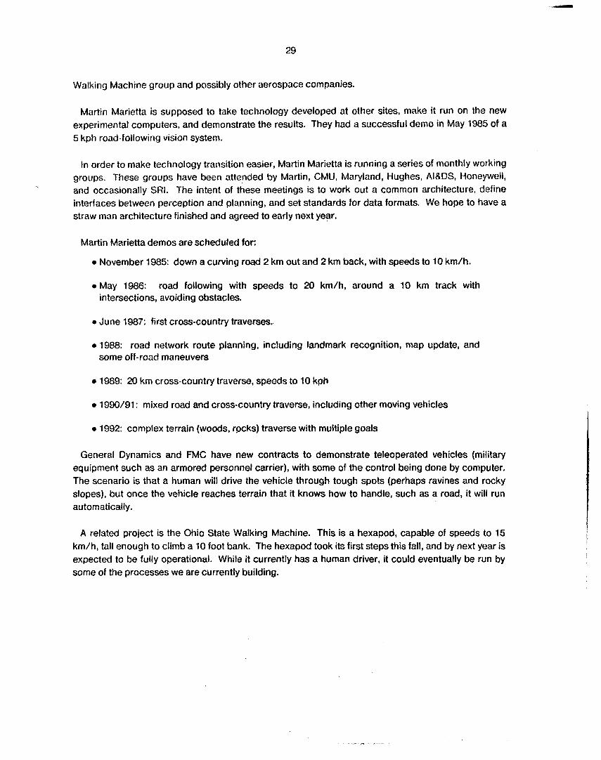
Walking Machine group and possibly other aerospace companies.

Martin Marietta is supposed to take technology developed at other sites, make it run on the new experimental computers, and demonstrate the results. They had a successful demo in May 1985 of a 5 kph road-following vision system.

In order to make technology transition easier, Martin Marietta is running a series of monthly working groups. These groups have been attended by Martin, CMU, Maryland, Hughes, AI&DS, Honeywell, and occasionally SRI. The intent of these meetings is to work out a common architecture, define interfaces between perception and planning, and set standards for data formats. We hope to have a straw man architecture finished and agreed to early next year.

Martin Marietta demos are scheduled for:

0 November 1985: down a curving road 2 km out and 2 km back, with speeds to 10 km/h.

0 May 1986: road following with speeds to 20 km/h, around a 10 km track with intersections, avoiding obstacles.

e June 1987: first cross-country traverses..

0 1988: road network route planning, including landmark recognition, map update, and some off-road maneuvers

0 1989: 20 km cross-country traverse, speeds to 10 kph

e 1990/91: mixed road and cross-country traverse, including other moving vehicles

0 1992: complex terrain (woods, rgcks) traverse with multiple goals

General Dynamics and FMC have new contracts to demonstrate teleoperated vehicles (military equipment such as an armored personnel carrier), with some of the control being done by computer. The scenario is that a human will drive the vehicle through tough spo?s (perhaps ravines and rocky slopes), but once the vehicle reaches terrain that it knows how to handle, such as a road, it will run automatically.

A related project is the Ohio State Walking Machine. This is a hexapod, capable of speeds to 15 km/h, tall enough to climb a 10 foot bank. The hexapod took its first steps this fall, and by next year is expected to be fully operational. While it currently has a human driver, it could eventually be run by some of the processes we are currently building.

30

4. History

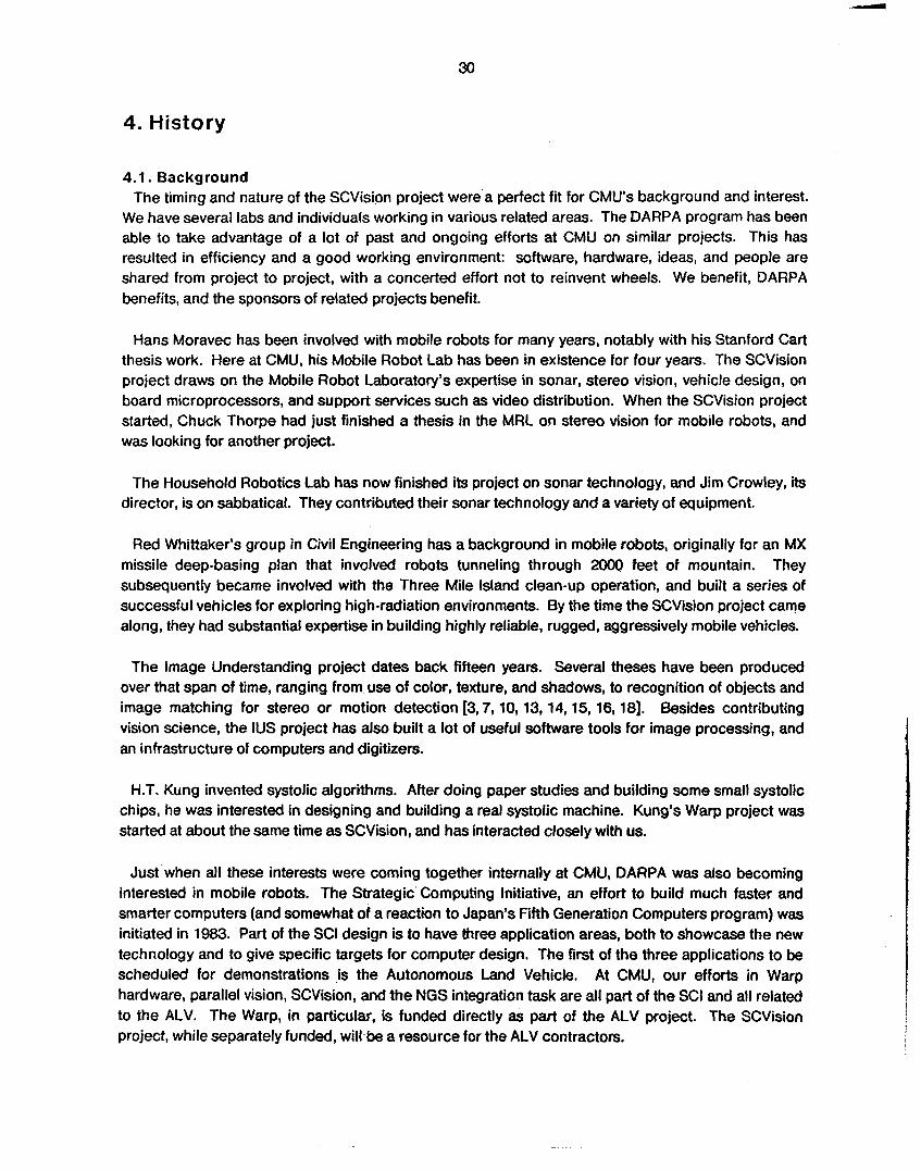
4.1. Background The timing and nature of the SCVision project were a perfect fit for CMU’s background and interest.

We have several labs and individuals working in various related areas. The DARPA program has been able to take advantage of a lot of past and ongoing efforts at CMU on similar projects. This has resulted in efficiency and a good working environment: software, hardware, ideas, and people are shared from project to project, with a concerted effort not to reinvent wheels. We benefit, DARPA benefits, and the sponsors of related projects benefit.

Hans Moravec has been involved with mobile robots for many years, notably with his Stanford Cart thesis work. Here at CMU, his Mobile Robot Lab has been in existence for four years. The SCVision project draws on the Mobile Robot Laboratory’s expertise in sonar, stereo vision, vehicle design, on board microprocessors, and support services such as video distribution. When the SCVision project started, Chuck Thorpe had just finished a thesis in the MRL on stereo vision for mobile robots, and was looking for another project.

The Household Robotics Lab has now finished its project on sonar technology, and Jim Crowley, its director, is on sabbatical. They contributed their sonar technology and a variety of equipment.

Red Whittaker’s group in Civil Engineering has a background in mobile robots, originally for an MX missile deep-basing plan that involved robots tunneling through 2OOO feet of mountain. They subsequently became involved with the Three Mile Island clean-up operation, and built a series of successful vehicles for exploring high-radiation environments. By the time the SCVision project came along, they had substantial expertise in building highly reliable, rugged, aggressively mobile vehicles.

The Image Understanding project dates back fifteen years. Several theses have been produced over that span of time, ranging from. use of color, texture, and shadows, to recognition of objects and image matching for stereo or motion detection [3,7,10,13,14, 15, 16,181. Besides contributing vision science, the IUS project has also built a lot of useful software tools for image processing, and an infrastructure of computers and digitizers.

H.T. Kung invented systolic algorithms. After doing paper studies and building some small systolic chips, he was interested in designing and building a real systolic machine. Kung’s Warp project was started at about the same time as SCVision, and has interacted closely with us.

Just when all these interests were coming together internally at CMU, DARPA was also becoming interested in mobile robots. The Strategic Computing Initiative, an effort to build much faster and smarter computers (and somewhat of a reaction to Japan’s Fifth Generation Computers program) was initiated in 1983. Part of the SCI design is to have three application areas, both to showcase the new technology and to give specific targets for computer design. The first of the three applications to be scheduled for demonstrations is the Autonomous Land Vehicle. At CMU, our efforts in Warp hardware, parallel vision, SCVision, and the NGS integration task are all part of the SCI and all related to the ALV. The Warp, in particular, is funded directly as part of the ALV project. The SCVision project, while separately funded, will be a resource for the ALV contractors.

31

4.2. Time line to date

0 January 84 Submit Qualification Statement on Image Understanding for SCVision

0 August 84 Submit Proposal for Research and Development of a Road-following Vision System

0 September 84 FlDO thesis defense (Thorpe)

0 September 84 First sonar mapping

0 October 84 Project starts

0 October 84 First Terregator runs under vision control (stop and go)

0 November 84 First successful indoor runs using sonar

0 November 84 First indoor continuous motion vision runs

0 December 84 First outdoor continuous motion vision runs

0 January 85 DARPA funding arrives

0 March 85 First outdoor vision runs with no tape marking edges

0 March 85 Vision runs using DOG, Roberts, row integration operators

0 March 85 First experience with Martin Marietta ERlM data

0 March 85 Blackboard proposed at an all-day meeting

0 May 85 ERlM scanner arrives at CMU

0 June 85 First outdoor sonar runs

0 June 85 Vision runs using rectification, row integration, and correlation

0 June through August 85 ERlM runs on sidewalks and in park collecting data

0 August 85 Blackboard document first circulated outside CMU

0 September 85 First Warp run; uses color to go 100 m at 112 km/h

0 September 85 Warp run up to 1 km/h for 180 meters on sidewalk

0 September 85 First successful ERlM run in park

0 September 85 Long sonar runs in outdoor environments

32

4.3. The Future We have two demos that we would like to do in Decernber, plus a variety of longer-term internal and

external commitments. The December demos are not for external purposes, but serve rather to define what we would like to accomplish internally.

Our first December demo will combine road following with obstacle avoidance on Flagstaff Hill. We want to use road following vision to drive the Terregator up the Flagstaff path and into the trees. Then, at some point (perhaps marked by a red cone) we will leave the path and strike off cross- country. We will use either ERIM, sonar, or stereo to avoid trees and other obstacles when off the road. The Terregator will eventually hit the road again, turn on to it, and resume road following. There may have to be another short off-road excursion to get around the steps at the far end of the hill by the drinking fountain. The run will conclude where the Flagstaff sidewalk hits Frew street and dead ends. This run will show the individual techniques of road following and obstacle avoidance. It nray also demonstrate landmark finding (in the simple case of finding cones) and road finding. If a map is used, it will be only in a limited sense. There will be no great attempt to combine information from multiple sensors into a single coherent framework. Instead, the road following and cross-country travel will be run as separate modes, with the only higher-level intelligence being used to switch from one mode to another.

The second December demo will be a map and planning demo. It will be a first complete system including the sensor and motion processing level and the local map level. The Terregator, thevehicle for this demo, will run on the sidewalks between Wean and Baker Halls, following the roads and turning on the intersections. The vision problem is easier (straight, white sidewalks against green grass) but the map problem is more difficult (a network of intersections and path segments). Planning and perception modules communicate with each other sending and receiving tokens, which include shapes and locations of predicted roads and intersections, detection strategy, detected line segments of roads and intersections, and map and vehicle position updates. Communication between the various modules looks like a dialogue; The main components to be demonstrated are vision for road and intersection detection, map modules, and the dialogue and architecture. The system used for this demo will be a first prototype of our complete system. Both of the December demos could use the Blackboard mechanisms i f they are available in time, or could run by themselves.

Our longer term goals include making full use of the blackboard, improving individual modules, and picking up speed. All these are tied together. If we build the Navlab, we would have multiple sensors going all the time. This will make the blackboard more necessary, which will in turn make it easier to integrate more modules. All those modules running together will mean that we will need more computing power. And having such an effective testbed will encourage and require that we improve the various modules in the system.

The blackboard will be ready for its first trials by the end of this year. It will initially be a bare bones package, without all the nice tools we would like. If we are selected as the NGS contractor, it will be expanded and improved based on input from other sites.

It is difficult to predict schedules for improvements of individual modules. Certainly, as we understand more about roads, and as we become more experienced with our color cameras, we will improve the quality of road following. We need to do more with combining ERIM data from view to

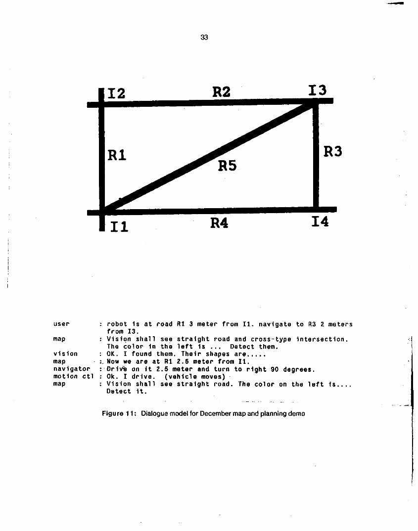
33

user : r o b o t i s a t road R 1 3 meter f r o m 11. nav iga te t o R3 2 meters

map : V i s i o n s h a l l see s t r a i g h t road and c ross- type i n t e r s e c t i o n .

v i s i o n : OK. I found them. T h e i r shapes are..... map . :,Now we a re a t R 1 2.5 meter f rom 11. n a v i g a t o r mot ion c t l : Ok. I d r i v e . ( v e h i c l e moves) map : V i s i o n s h a l l see s t r a i g h t road. The c o l o r on the l e f t i s . . . .

f rom 13.

The color i n t h e l e f t i s ... Detec t them.

: D r i 6 on i t 2.5 meter and t u r n t o r i g h t 90 degrees.

De tec t i t .

Figure 1 1 : Dialogue model for December map and planning demo

34

view, especially as we go cross-country. It is also time to begin looking at object recognition and characterization. It may take a combination of ERIM, sonar, and video data to distinguish a clump of grass from a rock, or to identify a particular building or rock outcrop. All of this is new research, and will be needed for cross-country work.

While our main emphasis is on handling increasingly difficult perception ‘tasks, we are also interested in running faster. We intend to acquire a Warp for our work, and to transfer software to our Warp. We have already done a run using a prototype Warp for simple vision, and have begun coding stereo vision and ERIM interpretation algorithms on the Warp.

5. People Mike Blackwell is a Research Engineer with the Mobile Robot Lab. He has been involved with the

SCVision project since the beginning, designing, building, and integrating hardware and low-level software for the various robots. He also makes sure things keep running, fixes them when they break, baby sits robots, and does all the billions of other little things that need to be done but nobody thinks about.

Jill Crisman is a Research Programmer for the Robotics Institute. She has been working on stereo vision and oriented road edge detection. Her main interests are household robotics and computer vision.

Kevin Dowliiig is a Research Engineer in the Robotics Institute and has been working in the Institute since its inception in 1980. He is involved in the design and construction of the mobile robots used in SCVision research. Telemetry, video, and hardware all seem to be areas of responsibility. His research interests are many, and include experiments in using control systems for visual servoing.

Alberto Elfes is a PhD Candidate and a Research Assistant in the Mobile Robot Lab. His present research focuses on software architectures for mobile robots, issues in cooperative problem-solving, sonar-based mapping and navigation, and planning and high-level control issues for autonomous robots.

Yoshimasa Goto is a visiting researcher in the Department of Computer Science. He is working on the map systems which predict and find objects, then revise the map data. His system will be used in the December map and planning demo. Research interests include knowledge based computer vision, inference and learning in vision, and shape representation.

Andy Gruss is Supervisor of Research Engineering in Computer Science. His responsibilities include setting up our lab and the care and feeding of our Suns. He is designing and building memory-mapped frame stores for Vaxes in his spare time.

Martial Hebert received his PhD from INRIA/University of Paris. He joined the SCVision project as a Visiting Scientist and is now a Research Associate. He works on range data analysis and 3-D map building for SCVision.

Ralph Hyre is a Research Programmer for the SCVision project, currently working on a debugging

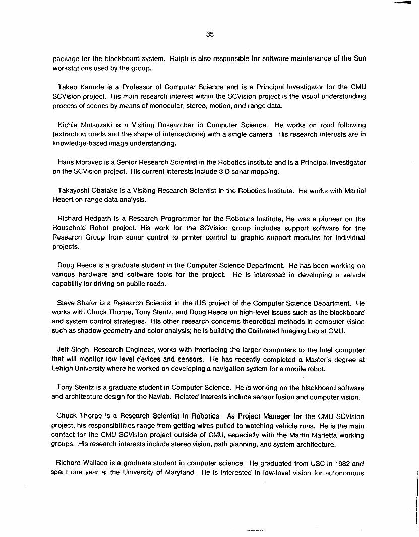
35

package for the blackboard system. Ralph is also responsible for software maintenance of the Sun workstations used by the group.

Takeo Kanade is a Professor of Computer Science and is a Principal Investigator for the CMU SCVisiori project. His main research interest within the SCVision project is the visual understanding process of scenes by means of monocular, stereo, motion, and range data.

Kichie Matsuzaki is a Visiting Researcher in Computer Science. He works on road following (extracting roads and the shape of intersections) with a single camera. His research interests are in knowledge-based image understanding.

Hans Moravec is a Senior Research Scientist in the Robotics Institute and is a Principal Investigator on the SCVision project. His current interests include 3-0 sonar mapping.

Takayoshi Obatake is a Visiting Research Scientist in the Robotics Institute. He works with Martial Hebert on range data analysis.

Richard Redpath is a Research Programmer for the Robotics Institute, He was a pioneer on the Household Robot project. His work for the SCVision group includes support software for the Research Group from sonar control to printer control to graphic support modules for individual projects.

Doug Reece is a graduate student in the Computer Science Department. He has been working on various hardware and software tools for the project. He is interested in developing a vehicle capability for driving on public roads.

Steve Shafer is a Research Scientist in the IUS project of the Computer Science Department. He works with Chuck Thorpe, Tony Stentz, and Doug Reece on high-level issues such as the blackboard and system control strategies. His other research concerns theoretical methods in computer vision such as shadow geometry and color analysis; he is building the Calibrated Imaging Lab at CMU.

Jeff Singh, Research Engineer, works with interfacing the larger computers to the Intel computer that will monitor low level devices and sensors. He has recently completed a Master’s degree at Lehigh University where he worked on developing a navigation system for a mobile robot.

Tony Stentz is a graduate student in Computer Science. He is working on the blackboard software and architecture design for the Navlab. Related interests include sensor fusion and computer vision.

Chuck Thorpe is a Research Scientist in Robotics. As Project Manager for the CMU SCVision project, his responsibilities range from getting wires pulled to watching vehicle runs. He is the main contact for the CMU SCVision project outside of CMU, especially with the Martin Marietta working groups. His research interests include stereo vision, path planning, and system architecture.

Richard Wallace is a graduate student in computer science. He graduated from USC in 1982 and spent one year at the University of Maryland. He is interested in low-level vision for autonomous

navigation.

Red Whittaker is an Assistant Professor in Civil Engineering and heads the Civil Engineering and Construction Robotics Lab. His work involves building real vehicles and their virtual vehicle interfaces. Besides the SCVision project, his lab builds highly reliable robots for nuclear power plant inspection and repair and for construction in hazardous sites.

6. Publications 10184 to 9/85 Elfes, A. E, Sonar Navigation, Workshop on Robotics, Oak Ridge National Lab, Oak Ridge, TN, August, 1985. (invited presentation)

0 Hebert, M. and T. Kanade: The 3-0 Profile Method for Object Recognition, Proc. Computer Vision and Pattern Recognition ‘85, San Francisco June 19-23 1985, pp. 458-464.

Kanade, T.: Image Understanding Research at CMU, Proc. DARPA Image Understanding Workshop, pp. 42-47, Oct. 1984, New Orleans.

e Moravec, H. P. and A. E. Elfes, High Resolution Maps from Wide Angle Sonar, proceeding of the 1985 IEEE International Conference on Robotics and Automation, St. Louis, March, 1985, pp 116-121, and proceedings of the 1985 ASME conference on Computers in Engineering, Boston, August, 1985.

0 Stentz, A, and S. Shafer. Module Programmer’s Guide to Local Map Builder for Navlab, Robotics Institute, Carnegie-Mellon University.

0 Stentz, A,, and C. Thorpe An Architecture for Autonomous Vehicle Navigation, Proceedings of the Fourth International Symposium on Unmanned Untethered Submersible Technology, Durham, NH, June, 1985.

oThorpe, C. E., FIDO: Vision and Navigation for a Mobile Robot, PhD Thesis, Computer Science Dept., Carnegie-Mellon University, December 1984. CMU CS Dept. Technical Report, 1985.

oThorpe, C., L. Matthies and H. Moravec, Experiments and Thoughts on Visual Navigation, the proceedings of the 1985 IEEE International Conference on Robotics and Automation, St. Louis, March, 1985, pp. 830-835.

0 Wallace, R. S., A Modified tiough Transform for’Lines, proceedings of the 1985 IEEE Conference on Vision and Pattern Recognition, San Francisco, June, 1985, pp. 665-667.

0 Wallace, R., A. Stentz, C. Thorpe, H. Moravec, W. Whittaker and T. Kanade, First Results in Robot Road-Following, proceedings of the 1985 IJCAI, Los Angeles, August, 1985 and proceedings of the 1985 ASME conference on Computers in Engineering, Boston, August, 1985.

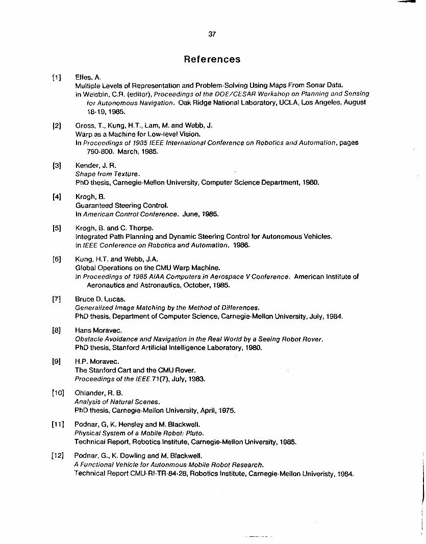
37

References

[l] Elfes, A. Multiple Levels of Representation and Problem-Solving Using Maps From Sonar Data. In Weisbin, C.R. (editor), Proceedings of the DOE/CESAR Workshop on Planning and Sensing

for Autonomous Navigation. Oak Ridge National Laboratory, UCLA, Los Angeles, August 18-19,1985.

[2] Gross, T., Kung, H.T., Lam, M. and Webb, J. Warp as a Machine for Low-level Vision. In Proceedings of 1935 IEEE International Conference on Robotics and Automation, pages

790-800. March, 1985.

[3] Kender, J. R. Shape from Texture. PhD thesis, Carnegie-Mellon University, Computer Science Department, 1980.

Guaranteed Steering Control. In American Control Conference. June, 1985.

Krogh, 6. and C. Thorpe. Integrated Path Planning and Dynamic Steering Control for Autonomous Vehicles. In IEEE Conference on Robotics and Automation. 1986.

[4] Krogh, 6.

[5]

[6] Kung, H.T. and Webb, J.A. Global Operations on the CMU Warp Machine. In Proceedings of 1985 AlAA Computers in Aerospace V Conference. American Institute of

Aeronautics and Astronautics, October, 1985.

[7] Bruce D. Lucas. Generalized Image Matching by the Method of Differences. PhD thesis, Department of Computer Science, Carnegie-Mellon University, July, 1984.

Obstacle Avoidance and Navigation in the Real World by a Seeing Robot Rover. PhD thesis, Stanford Artificial Intelligence Laboratory, 1980.

The Stanford Cart and the CMU Rover. Proceedings of the IEEE 71 (7), July, 1983.

[8] Hans Moravec.

[9] H.P. Moravec.

[lo] Ohlander, R. B. Analysis of Natural Scenes. PhD thesis, Carnegie-Mellon University, April, 1975.

Podnar, G, K. Hensley and M. Blackwell. Physical System of a Mobile Robot: Pluto. Technical Report, Robotics Institute, Carnegie-Mellon University, 1985.

Podnar, G., K. Dowling and M. Blackwell. A Functional Vehicle for Autonmous Mobile Robot Research. Technical Report CMU-RI-TR-84-28, Robotics Institute, Carnegie-Mellon Univeristy, 1984.

[ll]

[12]

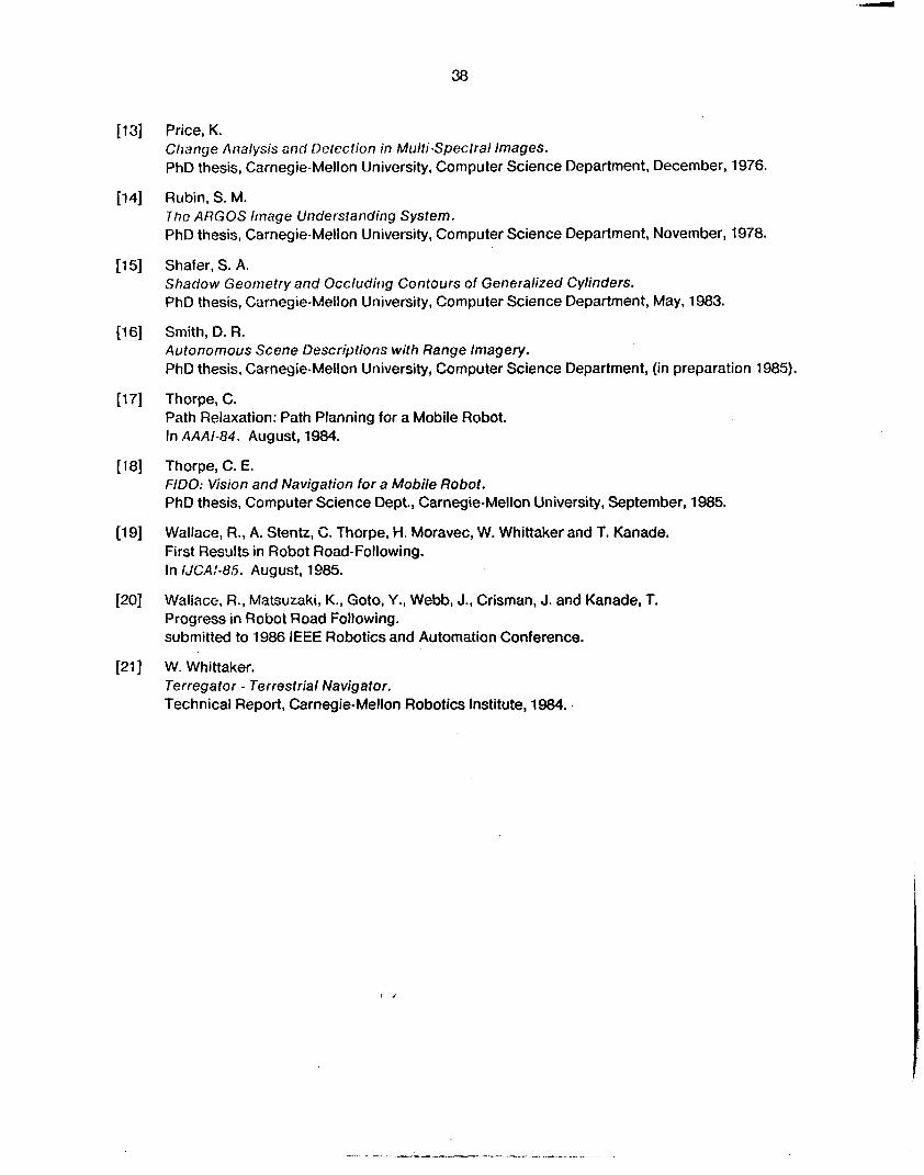
30

Price, K. Cliange Analysis and Detection in Multi-Spectral Images. PhD thesis, Carnegie-Mellon University, Computer Science Department, December, 1976.

Rubin, S. M. The ARGOS linage Understanding System. PhD thesis, Carnegie-Mellon University, Computer Science Department, November, 1978.

Shafer, S. A. Shadow Geometry and Occluditig Contours of Generalized Cylinders. PhD thesis, Carnegie-Meilon University, Computer Science Department, May, 1983.

Smith, D. R. Autonomous Scene Descriptions with Range Imagery. PhD thesis, Carnegie-Mellon University, Computer Science Department, (in preparation 1985).

Thorpe, C. Path Relaxation: Path Planning for a Mobile Robot. In AAAI-84. August, 1984.

Thorpe, C. E. FIDO: Vision and Navigation for a Mobile Robot. PhD thesis, Computer Science Dept., Carnegie-Mellon University, September, 1985.

Wallace, R., A. Stentz, C. Thorpe, H. Moravec, W. Whittaker and T. Kanade. First Results in Robot Road-Following. In iJCA:-85. August, 1985.

Waliace, R., Matsuzaki, K., Goto, Y., Webb, J., Crisman, J. and Kanade, T. Progress in Robot Road Following. submitted to 1986 IEEE Robotics and Automation Conference.

W. Whittaker. Terregator - Terrestrial Navigator. Technical Report, Carnegie-Mellon Robotics Institute, 1984. .