CM3120: Module 2

CM3120 Module 2 Lecture II 1/28/2021

1

CM3120: Module 2

© Faith A. Morrison, Michigan Tech U.1

Unsteady State Heat Transfer

I. IntroductionII. Unsteady Microscopic Energy Balance—(slash and burn)III. Unsteady Macroscopic Energy BalanceIV. Dimensional Analysis (unsteady)—Biot number, Fourier

numberV. Low Biot number solutions—Lumped parameter analysisVI. Short Cut Solutions—(initial temperature 𝑇 ; finite ℎ),

Gurney and Lurie charts (as a function of position, 𝑚

Bi, and Fo); Heissler charts (center point only, as a function of 𝑚 1/Bi, and Fo)

VII. Full Analytical Solutions (stretch)

CM3120: Module 2


Professor Faith A. Morrison

Department of Chemical EngineeringMichigan Technological University

www.chem.mtu.edu/~fmorriso/cm3120/cm3120.html

Module 2 Lecture II

Unsteady State Heat Transfer (Microscopic Energy Balances)


2


We model the dynamics of unsteady state heat transfer because there are very practical problems that we can

solve with such models.

Example:When will my pipes freeze?

The temperature has been 35oF for a while now, sufficient to chill the ground to this temperature for many tens of feet below the surface. Suddenly the temperature drops to ‐20oF. How long will it take for freezing temperatures (32oF) to reach my pipes, which are 8 ft under ground?

Ffth

BTUk

h

ft

Ffth

BTUh

osoil

soil

o

5.0

018.0

0.2

2

2


1/30/19


3

Example 1: Unsteady Heat Conduction in a Semi‐infinite solid

A very long, very wide, very tall slab is initially at a temperature𝑇 . At time 𝑡 0, the left face of the slab is exposed to a vigorously mixed gas at temperature 𝑇 . What is the time‐dependent temperature profile in the slab?


Unsteady State Heat Transfer: Dimensional Analysis

Develop a model:

Example: Unsteady Heat Conduction in a Semi‐infinite solid

x

y

z

HD

© Faith A. Morrison, Michigan Tech U.𝐻, 𝐷, very large

Unsteady State Heat Transfer

6


4

x

y

oTTt 0

oTTt 0

1

0TT

t 0

( , )

t

T T x t

x

y

© Faith A. Morrison, Michigan Tech U.

Initial Condition:

7

1D Heat Transfer: Unsteady State

Then,

General Energy Transport Equation(microscopic energy balance)

V

n̂dSS

As for the derivation of the microscopic momentum balance, the microscopic energy balance is derived on an arbitrary volume, V, enclosed by a surface, S.

STkTvtT

Cp

2ˆ

Gibbs notation:

see handout for component notation




5

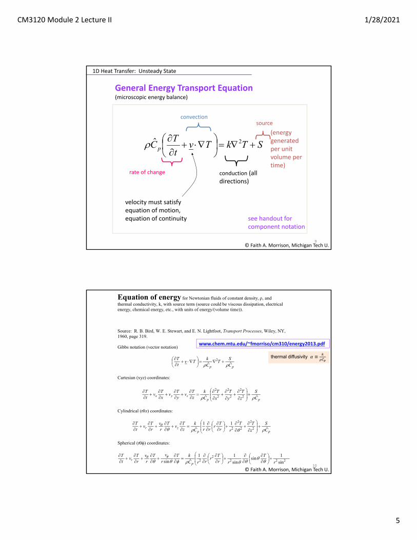
General Energy Transport Equation(microscopic energy balance)

see handout for component notation

rate of change

convection

conduction (all directions)

source

velocity must satisfy equation of motion, equation of continuity

(energy generated per unit volume per time)

STkTvt

TCp

2ˆ



www.chem.mtu.edu/~fmorriso/cm310/energy2013.pdf

Equation of energy for Newtonian fluids of constant density, , andthermal conductivity, k, with source term (source could be viscous dissipation, electricalenergy, chemical energy, etc., with units of energy/(volume time)).

CM310 Fall 1999 Faith Morrison

Source: R. B. Bird, W. E. Stewart, and E. N. Lightfoot, Transport Processes, Wiley, NY,1960, page 319.

Gibbs notation (vector notation)

pp C

ST

C

kTv

tT

ˆˆ2

Cartesian (xyz) coordinates:

ppzyx C

S

z

T

y

T

x

T

C

kzT

vyT

vxT

vtT

ˆˆ 2

2

2

2

2

2

Cylindrical (rz) coordinates:

ppzr C

S

z

TT

rrT

rrrC

kzT

vT

rv

rT

vtT

ˆ11

ˆ 2

2

2

2

2

Spherical (r) coordinates:

pr

r

T

rrT

rrrC

kTr

vTrv

rT

vtT

sin

1sin

sin

11ˆsin 222

22


thermal diffusivity 𝛼 ≡


6

Example 1: Unsteady Heat Conduction in a Semi‐infinite solid

A very long, very wide, very tall slab is initially at a temperature𝑇 . At time 𝑡 0, the left face of the slab is exposed to a vigorously mixed gas at temperature 𝑇 . What is the time‐dependent temperature profile in the slab?

© Faith A. Morrison, Michigan Tech U.

Newton’s law of cooling BC’s:

11

𝑞 ℎ𝐴 𝑇 𝑇 x

y

oTTt 0

oTTt 0

1

0TT

t 0

( , )

t

T T x t

x

y


ppzyx C

S

z

T

y

T

x

T

C

k

z

Tv

y

Tv

x

Tv

t

Tˆˆ 2

2

2

2

2

2

Microscopic Energy Equation in Cartesian Coordinates

pC

kˆ

thermal diffusivity

what are the boundary conditions? initial conditions?




7


Example: Unsteady Heat Conduction in a Semi‐infinite solid

You try.

x

y

oTTt 0

oTTt 0

1

0TT

t 0

( , )

t

T T x t

x

y

Initial Condition:


𝜕𝑇𝜕𝑡

𝑘

𝜌𝐶

𝜕 𝑇𝜕𝑥

𝛼𝜕 𝑇𝜕𝑥

Initial condition:

Boundary conditions:

Unsteady State Heat Conduction in a Semi‐Infinite Slab


x

y

oTTt 0

oTTt 0

1

0TT

t 0

( , )

t

T T x t

x

y1D Heat Transfer: Unsteady State

thermal diffusivity

𝛼 ≡𝑘

𝜌𝐶

𝑥 0𝑞𝐴

𝑘𝑑𝑇𝑑𝑥

ℎ 𝑇 𝑇 𝑡 0

𝑥 ∞ 𝑇 𝑇 ∀ 𝑡

𝑡 0 𝑇 𝑇 ∀ 𝑥


8

𝑥 0𝑞𝐴

𝑘𝑑𝑇𝑑𝑥

ℎ 𝑇 𝑇 𝑡 0

𝑥 ∞ 𝑇 𝑇 ∀ 𝑡

𝑡 0 𝑇 𝑇 ∀ 𝑥

© Faith A. Morrison, Michigan Tech U.© Faith A. Morrison, Michigan Tech U.15

x

y

oTTt 0

oTTt 0

1

0TT

t 0

( , )

t

T T x t

x

y

“for all 𝑡”


Initial condition:



thermal diffusivity

𝛼 ≡𝑘

𝜌𝐶

“for all 𝑥”Initial condition:


𝜕𝑇𝜕𝑡

𝛼𝜕 𝑇𝜕𝑥

𝑡 0 𝑇 𝑇 ∀ 𝑥Initial condition:


© Faith A. Morrison, Michigan Tech U.© Faith A. Morrison, Michigan Tech U.

k

th t

x

2

16


x

y

oTTt 0

oTTt 0

1

0TT

t 0

( , )

t

T T x t

x

y


See text WRF 6th ed p284 or BSL1 p353for the solution with temp BCs


9

𝑡 0 𝑇 𝑇 ∀ 𝑥Initial condition:


© Faith A. Morrison, Michigan Tech U.© Faith A. Morrison, Michigan Tech U.

k

th t

x

2

17


x

y

oTTt 0

oTTt 0

1

0TT

t 0

( , )

t

T T x t

x

y


See text WRF 6th ed p284 or BSL1 p353for the solution with temp BCs

• Geankoplis 4th ed., eqn 5.3‐7, page 363

• WRF, eqn 18‐21, page 286

k

th t

x

2

complementary error function of 𝒚

error function of 𝒚


𝑇 𝑇𝑇 𝑇

erfc 𝜁 𝑒 erfc 𝜁 𝛽

erfc 𝑦 ≡ 1 erf 𝑦

erf 𝑦 ≡2

𝜋𝑒 𝑑𝑦′

Solution:


(a standard function in Excel)

𝑌 ≡𝑇 𝑇𝑇 𝑇

1 𝑌𝑇 𝑇𝑇 𝑇

x

y

oTTt 0

oTTt 0

1

0TT

t 0

( , )

t

T T x t

x

y



10

k

th t

x

2

complementary error function of 𝒚

error function of 𝒚


𝑇 𝑇𝑇 𝑇


erfc 𝑦 ≡ 1 erf 𝑦

erf 𝑦 ≡2

𝜋𝑒 𝑑𝑦′

To make this solution easier to use, we can

plot it.

Solution:x

y

oTTt 0

oTTt 0

1

0TT

t 0

( , )

t

T T x t

x

yUnsteady State Heat Conduction in a Semi‐Infinite Slab





This:

Versus this:

At various values of this:

k

th

t

x

2

𝑇 𝑇𝑇 𝑇


To make this solution easier to use, we can

plot it.

x

y

oTTt 0

oTTt 0

1

0TT

t 0

( , )

t

T T x t

x

yUnsteady State Heat Conduction in a Semi‐Infinite Slab





11

0.01

0.1

1

0 0.4 0.8 1.2 1.6

1‐y

Zeta

20

3

2

1

0.6

0.4

0.3

0.2

0.1

0.07

0.05

t

x

2Plot design after

Geankoplis 4th ed., Figure 5.3‐3, page 364 ©

Faith A. M

orrison, M

ichigan

Tech U.

21





k

th

increasing 𝛽

𝛽 0.05

∞ 𝛽

0

0.1

0.2

0.3

0.4

0.5

0.6

0.7

0.8

0.9

1

0 2 4 6 8 10

x, ft

0.1

0.2

0.5

1

2

5

10

20

50

100

200

500

increasing time, t



With modern tools, we can plot the solution directly (evaluated in Excel)

1D Heat Transfer: Unsteady State Heat Conduction in a Semi‐Infinite Slab

ℎ 1.0

𝛼 1.0

𝑘 1.0 𝑓𝑡 𝐹

time, hrs


Direction of heat flux,

0


12

0

0.1

0.2

0.3

0.4

0.5

0.6

0.7

0.8

0.9

1

0 2 4 6 8 10

x, ft

0.1

0.2

0.5

1

2

5

10

20

50

100

200

500

increasing time, t



With modern tools, we can plot the solution directly (evaluated in Excel)


ℎ 1.0

𝛼 1.0


time, hrsNotice the steady‐state

effect of finite ℎ.


Example:When will my pipes freeze?

The temperature has been 35oF for a while now, sufficient to chill the ground to this temperature for many tens of feet below the surface. Suddenly the temperature drops to ‐20oF. How long will it take for freezing temperatures (32oF) to reach my pipes, which are 8 ft under ground?

Ffth

BTUk

h

ft

Ffth

BTUh

osoil

soil

o

5.0

018.0

0.2

2

2


1/30/19


13

Ffth

BTUk

h

ft

Ffth

BTUh

osoil

soil

o

5.0

018.0

0.2

2

2



We need the appropriate physical property data for

the soil.

Geankoplis 4th ed.



k

th

t

x

2

𝑇 𝑇𝑇 𝑇


𝑇 𝑇𝑇 𝑇

?

𝑇 ?𝑇 ?𝑇 ?

Both 𝜁and 𝛽depend on time


x

y

oTTt 0

oTTt 0

1

0TT

t 0

( , )

t

T T x t

x

y



Example: When will my pipes freeze?


14

t

x

2Geankoplis 4th ed., Figure

5.3‐3, page 364


𝛽




You try.

t

x

2Geankoplis 4th ed., Figure

5.3‐3, page 364


𝛽


Solution:



Guess large 𝛽(Interative solution)


15


𝑇 𝑇𝑇 𝑇


Answer:𝑡 480 ℎ𝑜𝑢𝑟𝑠 20 𝑑𝑎𝑦𝑠

x

y

oTTt 0

oTTt 0

1

0TT

t 0

( , )

t

T T x t

x

y





𝜁 ≡𝑥

2 𝛼𝑡


x

y

oTTt 0

oTTt 0

1

0TT

t 0

( , )

t

T T x t

x

y

Or, use Excel. (How exactly?)

𝑇 𝑇𝑇 𝑇


k

th

T0=

T1=

T=

h=

alpha=

k=

x=

Answer:𝑡 21.2 𝑑𝑎𝑦𝑠 𝛽 12.1

pages.mtu.edu/~fmorriso/cm310/2019PracticeProblemsInHeatTransfer%28Geankoplis%29.pdf



You try.


16

0

0.1

0.2

0.3

0.4

0.5

0.6

0.7

0.8

0.9

1

0 2 4 6 8 10

x, ft

0.1

0.2

0.5

1

2

5

10

20

50

100

200

500


With modern tools, we can plot the evolution of the model directly

(evaluated in Excel)

ℎ 2.0

𝛼 0.018


0.055 →

8𝑓𝑡

ℎ𝑜𝑢𝑟𝑠



aa_solutions/Unsteady semi infinite solid plots.xlsx

increasing time, t

𝑥,𝑓𝑡

‐20

‐10

0

10

20

30

40

‐2 0 2 4 6 8 10

x, ft

0.1 hours

0.2

0.5

1

2

5

10

20

50

100

200

500


With modern tools, we can plot the evolution of the model directly

(evaluated in Excel)

ℎ 2.0

𝛼 0.018


8𝑓𝑡



aa_solutions/Unsteady semi infinite solid plots.xlsx

increasing time, t

32 𝐹

𝑇 𝑥, 𝑡

𝑜 𝐹

𝑥,𝑓𝑡


17

‐20

‐10

0

10

20

30

40

‐2 0 2 4 6 8 10

x, ft

0.1 hours

0.2

0.5

1

2

5

10

20

50

100

200

500

8𝑓𝑡

increasing time, t

32 𝐹

𝑇 𝑥, 𝑡

𝑜 𝐹

𝑥, 𝑓𝑡


Solution Summary:

Answer:𝑡 509 ℎ𝑜𝑢𝑟𝑠 21 𝑑𝑎𝑦𝑠


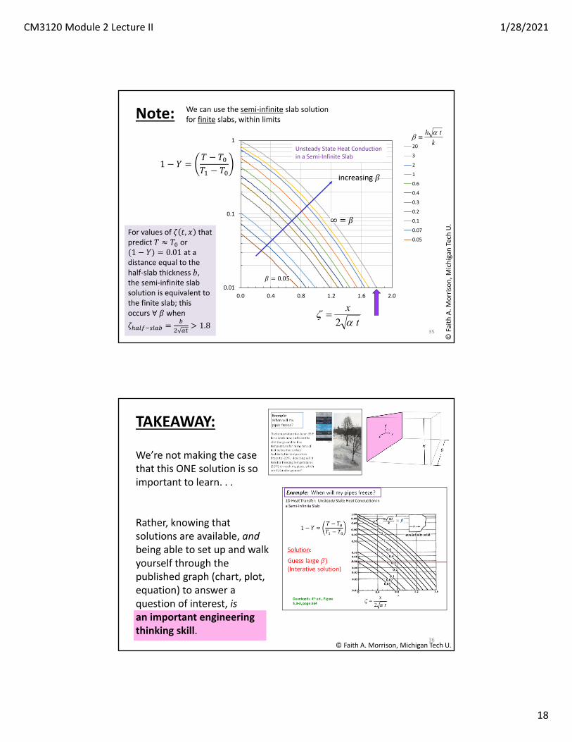
Note:

Finite SlabSemi‐Infinite Slab

BSL1, p356, 1960

We can use the semi‐infinite slab solution for finite slabs, within limits

0

0.1

0.2

0.3

0.4

0.5

0.6

0.7

0.8

0.9

1

0 2 4 6 8 10

x, ft

0.1

0.2

0.5

1

2

5

10

20

50

100

200

500

1𝑌

𝑇𝑇

𝑇𝑇

For some cases, the finite slab looks semi‐infinite

• Short time• Thicker slab


18

0.01

0.1

1

0.0 0.4 0.8 1.2 1.6 2.0

20

3

2

1

0.6

0.4

0.3

0.2

0.1

0.07

0.05

t

x

2

© Faith A. M

orrison, M

ichigan

Tech U.

35



k

th

increasing 𝛽

∞ 𝛽

𝛽 0.05

Note: We can use the semi‐infinite slab solution for finite slabs, within limits

For values of 𝜁 𝑡, 𝑥 that predict 𝑇 𝑇 or1 𝑌 0.01 at a distance equal to the half‐slab thickness 𝑏, the semi‐infinite slab solution is equivalent to the finite slab; this occurs ∀ 𝛽 when

𝜁 1.8


We’re not making the case that this ONE solution is so important to learn. . .

Rather, knowing that solutions are available, andbeing able to set up and walk yourself through the published graph (chart, plot, equation) to answer a question of interest, isan important engineering thinking skill.

TAKEAWAY:


19


We used the unsteady state microscopic energy balance to solve one practical problem.

Next, we explore the unsteady macroscopic energy balance.

This adds another tool to our tool belt.

Documents

CM3120: Module 2