Embed Size (px)
Citation preview

337
JJIIJI
Back
Close
Compression I:Basic Compression Algorithms
Recap: The Need for CompressionRaw Video, Image and Audio files are very large beasts:
Uncompressed Audio
1 minute of Audio:
Audio Type 44.1 KHz 22.05 KHz 11.025 KHz16 Bit Stereo 10.1 Mb 5.05 Mb 2.52 Mb16 Bit Mono 5.05 Mb 2.52 Mb 1.26 Mb8 Bit Mono 2.52 Mb 1.26 Mb 630 Kb

338
JJIIJI
Back
Close
Uncompressed Images
Image Type File Size512 x 512 Monochrome 0.25 Mb
512 x 512 8-bit colour image 0.25 Mb512 x 512 24-bit colour image 0.75 Mb

339
JJIIJI
Back
Close
Video
Can involve: Stream of audio and images
Raw Video – Uncompressed Image Frames, 512x512 TrueColor PAL 1125 Mb Per Min
DV Video — 200-300 Mb per Min (Approx) Compressed
HDTV — Gigabytes per second.
• Relying on higher bandwidths is not a good option — M25Syndrome.
• Compression HAS TO BE part of the representation ofaudio, image and video formats.

340
JJIIJI
Back
Close
Classifying Compression Algorithms
What is Compression?
Compression basically employs redundancy in the data:
• Temporal — in 1D data, 1D signals, Audio etc.
• Spatial — correlation between neighbouring pixels or dataitems
• Spectral — correlation between colour or luminescencecomponents.This uses the frequency domain to exploit relationshipsbetween frequency of change in data.
• Psycho-visual — exploit perceptual properties of the humanvisual system.

341
JJIIJI
Back
Close
Lossless v Lossy Compression
Compression can be categorised in two broad ways:
Lossless Compression — Entropy Encoding Schemes,LZW algorithm used in GIF image file format.
Lossy Compression — Source Coding Transform Coding,DCT used in JPEG/MPEG etc.
Lossy methods have to employed for image and videocompression:
• Compression ratio of lossless methods (e.g., Huffman Coding,Arithmetic Coding, LZW) is not high enough

342
JJIIJI
Back
Close
Lossless Compression Algorithms:Repetitive Sequence Suppression
• Fairly straight forward to understand and implement.
• Simplicity is their downfall: NOT best compression ratios.
• Some methods have their applications, e.g. Component ofJPEG, Silence Suppression.

343
JJIIJI
Back
Close
Simple Repetition Suppression
If a sequence a series on n successive tokens appears
• Replace series with a token and a count number ofoccurrences.
• Usually need to have a special flag to denote when therepeated token appears
For Example
89400000000000000000000000000000000
we can replace with
894f32
where f is the flag for zero.

344
JJIIJI
Back
Close
Simple Repetition Suppression: How Much Compression?
Compression savings depend on the content of the data.
Applications of this simple compression technique include:
• Suppression of zero’s in a file (Zero Length Suppression)
– Silence in audio data, Pauses in conversation etc.
– Bitmaps
– Blanks in text or program source files
– Backgrounds in images
• Other regular image or data tokens

345
JJIIJI
Back
Close
Lossless Compression Algorithms:Run-length Encoding
This encoding method is frequently applied to images(or pixels in a scan line).
It is a small compression component used inJPEG compression.
In this instance:
• Sequences of image elements X1, X2, . . . , Xn (Row by Row)
• Mapped to pairs (c1, l1), (c2, l2), . . . , (cn, ln)
where ci represent image intensity or colour and li the lengthof the ith run of pixels
• (Not dissimilar to zero length suppression above).

346
JJIIJI
Back
Close
Run-length Encoding Example
Original Sequence:111122233333311112222
can be encoded as:(1,4),(2,3),(3,6),(1,4),(2,4)
How Much Compression?
The savings are dependent on the data.
In the worst case (Random Noise) encoding is more heavythan original file:
2*integer rather 1* integer if data is represented as integers.

347
JJIIJI
Back
Close
Lossless Compression Algorithms:Pattern Substitution
This is a simple form of statistical encoding.
Here we substitute a frequently repeating pattern(s) with acode.
The code is shorter than than pattern giving uscompression.
A simple Pattern Substitution scheme could employ predefinedcodes

348
JJIIJI
Back
Close
Simple Pattern Substitution Example
For example replace all occurrences of ‘The’ with thepredefined code ’&’.
So:
The code is The Key
Becomes:
& code is & Key
Similar for other codes — commonly used words

349
JJIIJI
Back
Close
Token Assignment
More typically tokens are assigned to according to frequency ofoccurrence of patterns:
• Count occurrence of tokens
• Sort in Descending order
• Assign some symbols to highest count tokens
A predefined symbol table may used i.e. assign code i totoken T . (E.g. Some dictionary of common words/tokens)
However, it is more usual to dynamically assign codes to tokens.
The entropy encoding schemes below basically attempt todecide the optimum assignment of codes to achieve the bestcompression.

350
JJIIJI
Back
Close
Lossless Compression AlgorithmsEntropy Encoding
• Lossless Compression frequently involves some form ofentropy encoding
• Based on information theoretic techniques.

351
JJIIJI
Back
Close
Basics of Information Theory
According to Shannon, the entropy of an information source S
is defined as:
H(S) = η =∑
i pi log21pi
where pi is the probability that symbol Si in S will occur.
• log21pi
indicates the amount of information contained in Si,i.e., the number of bits needed to code Si.
• For example, in an image with uniform distribution of gray-levelintensity, i.e. pi = 1/256, then
– The number of bits needed to code each gray level is 8bits.
– The entropy of this image is 8.

352
JJIIJI
Back
Close
The Shannon-Fano Algorithm — Learn by Example
This is a basic information theoretic algorithm.
A simple example will be used to illustrate the algorithm:
A finite token Stream:ABBAAAACDEAAABBBDDEEAAA........
Count symbols in stream:
Symbol A B C D E----------------------------------
Count 15 7 6 6 5

353
JJIIJI
Back
Close
Encoding for the Shannon-Fano Algorithm:
• A top-down approach
1. Sort symbols (Tree Sort) according to theirfrequencies/probabilities, e.g., ABCDE.2. Recursively divide into two parts, each with approx. same
number of counts.

354
JJIIJI
Back
Close
3. Assemble code by depth first traversal of tree to symbolnode
Symbol Count log(1/p) Code Subtotal (# of bits)------ ----- -------- --------- -------------------
A 15 1.38 00 30B 7 2.48 01 14C 6 2.70 10 12D 6 2.70 110 18E 5 2.96 111 15
TOTAL (# of bits): 89
4. Transmit Codes instead of Tokens
• Raw token stream 8 bits per (39 chars) token = 312 bits
• Coded data stream = 89 bits

355
JJIIJI
Back
Close
Huffman Coding
• Based on the frequency of occurrence of a data item(pixels or small blocks of pixels in images).
• Use a lower number of bits to encode more frequent data
• Codes are stored in a Code Book — as for Shannon (previousslides)
• Code book constructed for each image or a set of images.
• Code book plus encoded data must be transmitted to enabledecoding.

356
JJIIJI
Back
Close
Encoding for Huffman Algorithm:
• A bottom-up approach
1. Initialization: Put all nodes in an OPEN list, keep it sortedat all times (e.g., ABCDE).
2. Repeat until the OPEN list has only one node left:(a) From OPEN pick two nodes having the lowest
frequencies/probabilities, create a parent node of them.(b) Assign the sum of the children’s frequencies/probabilities
to the parent node and insert it into OPEN.(c) Assign code 0, 1 to the two branches of the tree, and
delete the children from OPEN.

357
JJIIJI
Back
Close
Symbol Count log(1/p) Code Subtotal (# of bits)------ ----- -------- --------- --------------------
A 15 1.38 0 15B 7 2.48 100 21C 6 2.70 101 18D 6 2.70 110 18E 5 2.96 111 15
TOTAL (# of bits): 87

358
JJIIJI
Back
Close
The following points are worth noting about the above algorithm:
• Decoding for the above two algorithms is trivial as long asthe coding table/book is sent before the data.
– There is a bit of an overhead for sending this.
– But negligible if the data file is big.
• Unique Prefix Property: no code is a prefix to any othercode (all symbols are at the leaf nodes) –> great for decoder,unambiguous.
• If prior statistics are available and accurate, then Huffmancoding is very good.

359
JJIIJI
Back
Close
Huffman Entropy
In the above example:
Idealentropy = (15 ∗ 1.38 + 7 ∗ 2.48 + 6 ∗ 2.7
+6 ∗ 2.7 + 5 ∗ 2.96)/39
= 85.26/39
= 2.19
Number of bits needed for Huffman Coding is: 87/39 = 2.23

360
JJIIJI
Back
Close
Huffman Coding of Images
In order to encode images:
• Divide image up into (typically) 8x8 blocks
• Each block is a symbol to be coded
• Compute Huffman codes for set of block
• Encode blocks accordingly
• In JPEG: Blocks are DCT coded first before Huffman may beapplied (More soon)
Coding image in blocks is common to all image coding methods

361
JJIIJI
Back
Close
Adaptive Huffman Coding
Motivations:(a) The previous algorithms require prior statistical knowledge
• This may not be available
• E.g. live audio, video
(b) Even when stats dynamically available,
• Heavy overhead if many tables had to be sent — tables maychange drastically
• A non-order 0 model is used,
• I.e. taking into account the impact of the previous symbol tothe probability of the current symbol can improve efficiency.
• E.g., ”qu” often come together, ....

362
JJIIJI
Back
Close
Solution: Use adaptive algorithms
As an example, the Adaptive Huffman Coding is examinedbelow.
The idea is however applicable to other adaptive compressionalgorithms.
ENCODER DECODER------- -------
Initialize_model(); Initialize_model();while ((c = getc (input)) while ((c = decode (input))!= eof) != eof)
{ {encode (c, output); putc (c, output);update_model (c); update_model (c);
} }

363
JJIIJI
Back
Close
• Key: encoder and decoder use same initialization andupdate model routines.
• update model does two things:(a) increment the count,(b) update the Huffman tree.
– During the updates, the Huffman tree will be maintained
– its sibling property, i.e. the nodes (internal and leaf) arearranged in order of increasing weights.
– When swapping is necessary, the farthest node with weightW is swapped with the node whose weight has just beenincreased to W+1.
– Note: If the node with weight W has a subtree beneath it,then the subtree will go with it.
– The Huffman tree could look very different after swapping

364
JJIIJI
Back
Close

365
JJIIJI
Back
Close
Arithmetic Coding
• A widely used entropy coder
• Also used in JPEG — more soon
• Only problem is it’s speed due possibly complex computationsdue to large symbol tables,
• Good compression ratio (better than Huffman coding),entropy around the Shannon Ideal value.
Why better than Huffman?
• Huffman coding etc. use an integer number (k) of bits foreach symbol,
– hence k is never less than 1.
• Sometimes, e.g., when sending a 1-bit image, compressionbecomes impossible.

366
JJIIJI
Back
Close
Decimal Static Arithmetic Coding
• Here we describe basic approach of Arithmetic Coding
• Initially basic static coding mode of operation.
• Initial example decimal coding
• Extend to Binary and then machine word length later

367
JJIIJI
Back
Close
Basic Idea
The idea behind arithmetic coding is
• To have a probability line, 0–1, and
• Assign to every symbol a range in this line based on itsprobability,
• The higher the probability, the higher range which assigns toit.
Once we have defined the ranges and the probability line,
• Start to encode symbols,
• Every symbol defines where the output floating point numberlands within the range.

368
JJIIJI
Back
Close
Simple Basic Arithmetic Coding Example
Assume we have the following token symbol stream
BACA
Therefore
• A occurs with probability 0.5,
• B and C with probabilities 0.25.

369
JJIIJI
Back
Close
Basic Arithmetic Coding Clgorithm
Start by assigning each symbol to the probability range 0–1.
• Sort symbols highest probability first
Symbol RangeA [0.0, 0.5)B [0.5, 0.75)C [0.75, 1.0)
The first symbol in our example stream is B
• We now know that the code will be in the range 0.5 to 0.74999 . . ..

370
JJIIJI
Back
Close
Range is not yet unique
• Need to narrow down the range to give us a unique code.
Basic arithmetic coding iteration
• Subdivide the range for the first token given the probabilitiesof the second token then the third etc.

371
JJIIJI
Back
Close
Subdivide the range as follows
For all the symbols
• Range = high - low
• High = low + range * high range of the symbol being coded
• Low = low + range * low range of the symbol being coded
Where:
• Range, keeps track of where the next range should be.
• High and low, specify the output number.
• Initially High = 1.0, Low = 0.0

372
JJIIJI
Back
Close
Back to our example
The second symbols we have(now Range = 0.25, Low = 0.5, High = 0.75):
Symbol RangeBA [0.5, 0.625)BB [0.625, 0.6875)BC [0.6875, 0.75)
373
JJIIJI
Back
Close
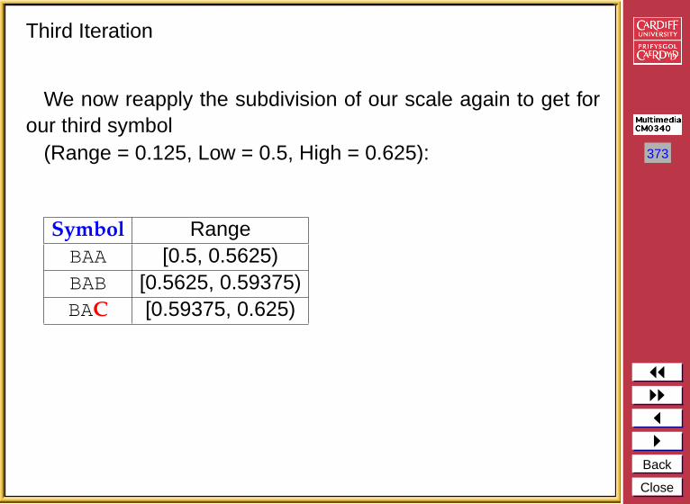
Third Iteration
We now reapply the subdivision of our scale again to get forour third symbol
(Range = 0.125, Low = 0.5, High = 0.625):
Symbol RangeBAA [0.5, 0.5625)BAB [0.5625, 0.59375)BAC [0.59375, 0.625)

374
JJIIJI
Back
Close
Fourth Iteration
Subdivide again(Range = 0.03125, Low = 0.59375, High = 0.625):
Symbol RangeBACA [0.59375, 0.60937)BACB [0.609375, 0.6171875)BACC [0.6171875, 0.625)
So the (Unique) output code for BACAis any number in therange:
[0.59375, 0.60937).

375
JJIIJI
Back
Close
Decoding
To decode is essentially the opposite
• We compile the table for the sequence given probabilities.
• Find the range of number within which the code number liesand carry on

376
JJIIJI
Back
Close
Binary static algorithmic coding
This is very similar to above:
• except we us binary fractions.
Binary fractions are simply an extension of the binary systemsinto fractions much like decimal fractions.

377
JJIIJI
Back
Close
Binary Fractions — Quick Guide
Fractions in decimal:
0.1 decimal = 1101 = 1/10
0.01 decimal = 1102 = 1/100
0.11 decimal = 1101 + 1
102 = 11/100
So in binary we get
0.1 binary = 121 = 1/2 decimal
0.01 binary = 122 = 1/4 decimal
0.11 binary = 121 + 1
22 = 3/4 decimal

378
JJIIJI
Back
Close
Binary Arithmetic Coding Example
• Idea: Suppose alphabet was X, Y and token stream:
XXY
Therefore:
prob(X) = 2/3prob(Y) = 1/3
• If we are only concerned with encoding length 2 messages,then we can map all possible messages to intervals in therange [0..1]:

379
JJIIJI
Back
Close
• To encode message, just send enough bits of a binary fractionthat uniquely specifies the interval.

380
JJIIJI
Back
Close
• Similarly, we can map all possible length 3 messages tointervals in the range [0..1]:

381
JJIIJI
Back
Close
Implementation Issues
FPU Precision
• Resolution of the of the number we represent is limited byFPU precision
• Binary coding extreme example of rounding
• Decimal coding is the other extreme — theoretically norounding.
• Some FPUs may us up to 80 bits
• As an example let us consider working with 16 bit resolution.

382
JJIIJI
Back
Close
16-bit arithmetic coding
We now encode the range 0–1 into 65535 segments:
0.000 0.250 0.500 0,750 1.0000000h 4000h 8000h C000h FFFFh
If we take a number and divide it by the maximum (FFFFh) wewill clearly see this:
0000h: 0/65535 = 0.04000h: 16384/65535 = 0.258000h: 32768/65535 = 0.5C000h: 49152/65535 = 0.75FFFFh: 65535/65535 = 1.0

383
JJIIJI
Back
Close
The operation of coding is similar to what we have seen withthe binary coding:
• Adjust the probabilities so the bits needed for operating withthe number aren’t above 16 bits.
• Define a new interval
• The way to deal with the infinite number is
– to have only loaded the 16 first bits, and when neededshift more onto it:1100 0110 0001 000 0011 0100 0100 ...
– work only with those bytes
– as new bits are needed they’ll be shifted.

384
JJIIJI
Back
Close
Memory Problems
What about an alphabet with 26 symbols, or 256 symbols, ...?
• In general, number of bits is determined by the size of theinterval.
• In general, (from entropy) need− log p bits to represent intervalof size p.
• Can be memory and CPU intensive

385
JJIIJI
Back
Close
Estimating Probabilities - Dynamic Arithmetic Coding?
How to determine probabilities?
• If we have a static stream we simply count the tokens.
Could use a priori information for static or dynamic if scenariofamiliar.
But for Dynamic Data?
• Simple idea is to use adaptive model:
– Start with guess of symbol frequencies — or all equalprobabilities
– Update frequency with each new symbol.
• Another idea is to take account of intersymbol probabilities,e.g., Prediction by Partial Matching.

386
JJIIJI
Back
Close
Lempel-Ziv-Welch (LZW) Algorithm
• A very common compression technique.
• Used in GIF files (LZW), UNIX compress (LZ Only)
• Patented — LZW not LZ.
Basic idea/Example by Analogy:Suppose we want to encode the Oxford Concise English
dictionary which contains about 159,000 entries.
Why not just transmit each word as an 18 bit number?

387
JJIIJI
Back
Close
Problems:
• Too many bits,
• Everyone needs a dictionary,
• Only works for English text.
Solution:
• Find a way to build the dictionary adaptively.
• Original methods (LZ) due to Lempel and Ziv in 1977/8.
• Terry Welch improved the scheme in 1984,P¯atented LZW Algorithm

388
JJIIJI
Back
Close
LZW Compression Algorithm
The LZW Compression Algorithm can summarised as follows:
w = NIL;while ( read a character k )
{if wk exists in the dictionary
w = wk;else
{ add wk to the dictionary;output the code for w;
w = k;}
}
• Original LZW used dictionary with 4K entries, first 256 (0-255)are ASCII codes.

389
JJIIJI
Back
Close
Example:Input string is "ˆWEDˆWEˆWEEˆWEBˆWET".
w k output index symbol-----------------------------------------
NIL ˆˆ W ˆ 256 ˆWW E W 257 WEE D E 258 EDD ˆ D 259 Dˆˆ W
ˆW E 256 260 ˆWEE ˆ E 261 Eˆˆ W
ˆW EˆWE E 260 262 ˆWEE
E ˆEˆ W 261 263 EˆW
W EWE B 257 264 WEB
B ˆ B 265 Bˆˆ W
ˆW EˆWE T 260 266 ˆWET
T EOF T
• A 19-symbol inputhas been reducedto 7-symbol plus5-code output. Eachcode/symbol willneed more than 8bits, say 9 bits.
• Usually,compressiondoesn’t start untila large number ofbytes (e.g., > 100)are read in.

390
JJIIJI
Back
Close
LZW Decompression Algorithm
The LZW Decompression Algorithm is as follows:
read a character k;output k;w = k;while ( read a character k )/* k could be a character or a code. */
{entry = dictionary entry for k;output entry;add w + entry[0] to dictionary;w = entry;
}

391
JJIIJI
Back
Close
Example (continued):
Input string is"ˆWED<256>E<260><261><257>B<260>T"
w k output index symbol----------------------------------------
ˆ ˆˆ W W 256 ˆWW E E 257 WEE D D 258 EDD <256> ˆW 259 Dˆ
<256> E E 260 ˆWEE <260> ˆWE 261 Eˆ
<260> <261> Eˆ 262 ˆWEE<261> <257> WE 263 EˆW<257> B B 264 WEB
B <260> ˆWE 265 Bˆ<260> T T 266 ˆWET

392
JJIIJI
Back
Close
Problems?
• What if we run out of dictionary space?
– Solution 1: Keep track of unused entries and use LRU
– Solution 2: Monitor compression performance and flushdictionary when performance is poor.
• Implementation Note: LZW can be made really fast;
– it grabs a fixed number of bits from input stream,
– so bit parsing is very easy.
– Table lookup is automatic.

393
JJIIJI
Back
Close
Entropy Encoding Summary
• Huffman maps fixed length symbols to variable length codes.Optimal only when symbol probabilities are powers of 2.
• Arithmetic maps entire message to real number range basedon statistics. Theoretically optimal for long messages, butoptimality depends on data model. Also can be CPU/memoryintensive.
• Lempel-Ziv-Welch is a dictionary-based compression method.It maps a variable number of symbols to a fixed length code.
• Adaptive algorithms do not need a priori estimation ofprobabilities, they are more useful in real applications.
394
JJIIJI
Back
Close
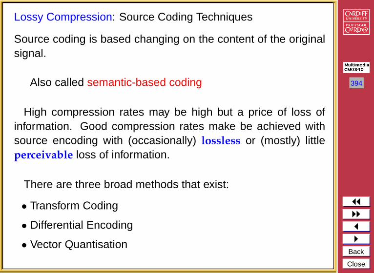
Lossy Compression: Source Coding Techniques
Source coding is based changing on the content of the originalsignal.
Also called semantic-based coding
High compression rates may be high but a price of loss ofinformation. Good compression rates make be achieved withsource encoding with (occasionally) lossless or (mostly) littleperceivable loss of information.
There are three broad methods that exist:
• Transform Coding
• Differential Encoding
• Vector Quantisation

395
JJIIJI
Back
Close
Transform Coding
A simple transform coding example
A Simple Transform Encoding procedure maybe described bythe following steps for a 2x2 block of monochrome pixels:
1. Take top left pixel as the base value for the block, pixel A.
2. Calculate three other transformed values by taking thedifference between these (respective) pixels and pixel A,Ii.e. B-A, C-A, D-A.
3. Store the base pixel and the differences as the values of thetransform.

396
JJIIJI
Back
Close
Simple Transforms
Given the above we can easily form the forward transform:
X0 = A
X1 = B − A
X2 = C − A
X3 = D − A
and the inverse transform is:
An = X0
Bn = X1 + X0
Cn = X2 + X0
Dn = X3 + X0

397
JJIIJI
Back
Close
Compressing data with this Transform?
Exploit redundancy in the data:
• Redundancy transformed to values, Xi.
• Compress the data by using fewer bits to represent thedifferences.
– I.e if we use 8 bits per pixel then the 2x2 block uses 32bits
– If we keep 8 bits for the base pixel, X0,
– Assign 4 bits for each difference then we only use 20 bits.
– Better than an average 5 bits/pixel

398
JJIIJI
Back
Close
Example
Consider the following 4x4 image block:
120 130125 120
then we get:
X0 = 120
X1 = 10
X2 = 5
X3 = 0
We can then compress these values by taking less bits torepresent the data.

399
JJIIJI
Back
Close
Inadequacies of Simple Scheme
• It is Too Simple
• Needs to operate on larger blocks (typically 8x8 min)
• Simple encoding of differences for large values will result inloss of information
– V. poor losses possible here 4 bits per pixel = values 0-15unsigned,
– Signed value range: −7 – 7 so either quantise in multiplesof 255/max value or massive overflow!!
• More advance transform encoding techniques are verycommon – DCT
400
JJIIJI
Back
Close
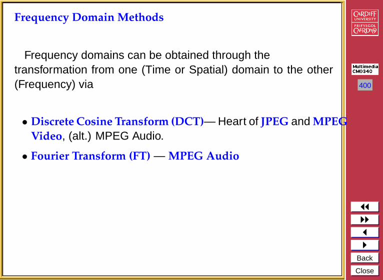
Frequency Domain Methods
Frequency domains can be obtained through thetransformation from one (Time or Spatial) domain to the other(Frequency) via
• Discrete Cosine Transform (DCT)— Heart of JPEG and MPEGVideo, (alt.) MPEG Audio.
• Fourier Transform (FT) — MPEG Audio

401
JJIIJI
Back
Close
1D Example
Lets consider a 1D (e.g. Audio) example to see what the differentdomains mean:
Consider a complicated sound such as the noise of a carhorn. We can describe this sound in two related ways:
• Sample the amplitude of the sound many times a second,which gives an approximation to the sound as a function oftime.
• Analyse the sound in terms of the pitches of the notes, orfrequencies, which make the sound up, recording theamplitude of each frequency.

402
JJIIJI
Back
Close
An 8Hz Sine Wave
In the example (next slide):
• A signal that consists of a sinusoidal wave at 8 Hz.
• 8Hz means that wave is completing 8 cycles in 1 second
• The frequency of that wave (8 Hz).
• From the frequency domain we can see that the compositionof our signal is
– one wave (one peak) occurring with a frequency of 8Hz
– with a magnitude/fraction of 1.0 i.e. it is the whole signal.

403
JJIIJI
Back
Close
An 8Hz Sine Wave (Cont.)

404
JJIIJI
Back
Close
2D Image Example
Now images are no more complex really:
• Brightness along a line can be recorded as a set of valuesmeasured at equally spaced distances apart,
• Or equivalently, at a set of spatial frequency values.
• Each of these frequency values is a frequency component.
• An image is a 2D array of pixel measurements.
• We form a 2D grid of spatial frequencies.
• A given frequency component now specifies what contributionis made by data which is changing with specified x and y
direction spatial frequencies.

405
JJIIJI
Back
Close
What do frequencies mean in an image?
• Large values at high frequency components then the datais changing rapidly on a short distance scale.
e.g. a page of text
• Large low frequency components then the large scale featuresof the picture are more important.
e.g. a single fairly simple object which occupies most of theimage.

406
JJIIJI
Back
Close
So How Compress (colour) images?
• The 2D matrix of the frequency content is with regard tocolour/chrominance:
• This shows if values are changing rapidly or slowly.
• Where the fraction, or value in the frequency matrix is low,the colour is changing gradually.
• Human eye is insensitive to gradual changes in colour andsensitive to intensity.
• Ignore gradual changes in colour SO
• Basic Idea: Attempt to throw away data without the humaneye noticing, we hope.

407
JJIIJI
Back
Close
How can transforms into the Frequency Domain Help to Compress?
Any function (signal) can be decomposed into purely sinusoidalcomponents (sine waves of different size/shape) which whenadded together make up our original signal.
Figure 39: DFT of a Square Wave

408
JJIIJI
Back
Close
Thus Transforming a signal into the frequency domain allowsus
• To see what sine waves make up our underlying signal
• E.g.
– One part sinusoidal wave at 50 Hz and
– Second part sinusoidal wave at 200 Hz.
More complex signals will give more complex graphs but theidea is exactly the same. The graph of the frequency domain iscalled the frequency spectrum.

409
JJIIJI
Back
Close
Visualising this: Think Graphic Equaliser
An easy way to visualise what is happening is to think of agraphic equaliser on a stereo.
Figure 40: A Graphic Equaliser

410
JJIIJI
Back
Close
Fourier Theory
The tool which converts a spatial (real space) description ofan image into one in terms of its frequency components is calledthe Fourier transform
The new version is usually referred to as the Fourier spacedescription of the image.
The corresponding inverse transformation which turns a Fourierspace description back into a real space one is called the
inverse Fourier transform.

411
JJIIJI
Back
Close
1D Case
Considering a continuous function f (x) of a single variable x
representing distance.
The Fourier transform of that function is denoted F (u), whereu represents spatial frequency is defined by
F (u) =
∫ ∞
−∞f (x)e−2πixu dx. (1)
Note: In general F (u) will be a complex quantity even thoughthe original data is purely real.
The meaning of this is that not only is the magnitude of eachfrequency present important, but that its phase relationship istoo.

412
JJIIJI
Back
Close
Inverse 1D Fourier Transform
The inverse Fourier transform for regenerating f (x) from F (u) isgiven by
f (x) =
∫ ∞
−∞F (u)e2πixu du, (2)
which is rather similar, except that the exponential term hasthe opposite sign.

413
JJIIJI
Back
Close
Example Fourier Transform
Let’s see how we compute a Fourier Transform: consider aparticular function f (x) defined as
f (x) =
{1 if |x| ≤ 1
0 otherwise,(3)
Figure 41: A top hat function

414
JJIIJI
Back
Close
So its Fourier transform is:
F (u) =
∫ ∞
−∞f (x)e−2πixu dx
=
∫ 1
−1
1× e−2πixu dx
=−1
2πiu(e2πiu − e−2πiu)
=sin 2πu
πu. (4)
In this case F (u) is purely real, which is a consequence of theoriginal data being symmetric in x and −x.
A graph of F (u) is shown overleaf.
This function is often referred to as the Sinc function.

415
JJIIJI
Back
Close
The Sync Function
Figure 42: Fourier transform of a top hat function

416
JJIIJI
Back
Close
2D Case
If f (x, y) is a function, for example the brightness in an image,its Fourier transform is given by
F (u, v) =
∫ ∞
−∞
∫ ∞
−∞f (x, y)e−2πi(xu+yv) dx dy, (5)
and the inverse transform, as might be expected, is
f (x, y) =
∫ ∞
−∞
∫ ∞
−∞F (u, v)e2πi(xu+yv) du dv. (6)

417
JJIIJI
Back
Close
Images are digitised !!
Thus, we need a discrete formulation of the Fourier transform,which takes such regularly spaced data values, and returns thevalue of the Fourier transform for a set of values in frequencyspace which are equally spaced.
This is done quite naturally by replacing the integral by asummation, to give the discrete Fourier transform or DFT forshort.
In 1D it is convenient now to assume that x goes up in stepsof 1, and that there are N samples, at values of x from 0 to N−1.

418
JJIIJI
Back
Close
1D Discrete Fourier transform
So the DFT takes the form
F (u) =1
N
N−1∑x=0
f (x)e−2πixu/N , (7)
while the inverse DFT is
f (x) =
N−1∑x=0
F (u)e2πixu/N . (8)
NOTE: Minor changes from the continuous case are a factorof 1/N in the exponential terms, and also the factor 1/N in frontof the forward transform which does not appear in the inversetransform.

419
JJIIJI
Back
Close
2D Discrete Fourier transform
The 2D DFT works is similar. So for an N ×M grid in x and y
we have
F (u, v) =1
NM
N−1∑x=0
M−1∑y=0
f (x, y)e−2πi(xu/N+yv/M), (9)
and
f (x, y) =
N−1∑u=0
M−1∑v=0
F (u, v)e2πi(xu/N+yv/M). (10)

420
JJIIJI
Back
Close
Balancing the 2D DFT
Often N = M , and it is then it is more convenient to redefineF (u, v) by multiplying it by a factor of N , so that the forward andinverse transforms are more symmetrical:
F (u, v) =1
N
N−1∑x=0
N−1∑y=0
f (x, y)e−2πi(xu+yv)/N , (11)
and
f (x, y) =1
N
N−1∑u=0
N−1∑v=0
F (u, v)e2πi(xu+yv)/N . (12)

421
JJIIJI
Back
Close
Compression
How do we achieve compression?
• Low pass filter — ignore high frequency noise components
• Only store lower frequency components
• High Pass Filter — Spot Gradual Changes
• If changes to low Eye does not respond so ignore?
Where do put threshold to cut off?

422
JJIIJI
Back
Close
Relationship between DCT and FFT
DCT (Discrete Cosine Transform) is actually a cut-down versionof the FFT:
• Only the real part of FFT
• Computationally simpler than FFT
• DCT — Effective for Multimedia Compression
• DCT MUCH more commonly used in Multimedia.

423
JJIIJI
Back
Close
The Discrete Cosine Transform (DCT)
• Similar to the discrete Fourier transform:
– it transforms a signal or image from the spatial domain tothe frequency domain
– DCT can approximate lines well with fewer coefficients
Figure 43: DCT Encoding
• Helps separate the image into parts (or spectral sub-bands)of differing importance (with respect to the image’s visualquality).

424
JJIIJI
Back
Close
1D DCT
For N data items 1D DCT is defined by:
F (u) =
(2
N
)12 N−1∑
i=0
Λ(i).cos[ π.u
2.N(2i + 1)
]f (i)
and the corresponding inverse 1D DCT transform is simpleF−1(u), i.e.:
f (i) = F−1(u)
=
(2
N
)12 N−1∑
i=0
Λ(i).cos[ π.u
2.N(2i + 1)
]F (i)
where
Λ(i) =
{1√2
forξ = 0
1 otherwise

425
JJIIJI
Back
Close
2D DCT
For a 2D N by M image 2D DCT is defined :
F (u, v) =
(2
N
) 12(
2
M
) 12
N−1∑i=0
M−1∑j=0
Λ(i).Λ(j).
cos[ π.u
2.N(2i + 1)
]cos
[ π.v
2.M(2j + 1)
].f(i, j)
and the corresponding inverse 2D DCT transform is simple F−1(u, v),i.e.:
f(i) = F−1(u, v)
=
(2
N
) 12
N−1∑i=0
M−1∑j=0
Λ(i)..Λ(j).
cos[ π.u
2.N(2i + 1)
].cos
[ π.v
2.M(2j + 1)
].F (i, j)
where
Λ(ξ) =
{1√2
forξ = 0
1 otherwise

426
JJIIJI
Back
Close
Performing DCT Computations
The basic operation of the DCT is as follows:
• The input image is N by M;
• f(i,j) is the intensity of the pixel in row i and column j;
• F(u,v) is the DCT coefficient in row k1 and column k2 of theDCT matrix.
• The DCT input is an 8 by 8 array of integers.This array contains each image window’s gray scale pixellevels;
• 8 bit pixels have levels from 0 to 255.

427
JJIIJI
Back
Close
Compression with DCT for Compression
• For most images, much of the signal energy lies at lowfrequencies;
– These appear in the upper left corner of the DCT.
• Compression is achieved since the lower right valuesrepresent higher frequencies, and are often small
– Small enough to be neglected with little visible distortion.

428
JJIIJI
Back
Close
Computational Issues (1)
• Image is partitioned into 8 x 8 regions — The DCT input isan 8 x 8 array of integers.
• An 8 point DCT would be:
F (u, v) =1
4
∑i,j
Λ(i).Λ(j).cos[π.u
16(2i + 1)
].
cos[π.u
16(2i + 1)
]f (i, j)
where
Λ(ξ) =
{ 1√2 forξ = 0
1 otherwise
• The output array of DCT coefficients contains integers; these canrange from -1024 to 1023.

429
JJIIJI
Back
Close
Computational Issues (2)
• Computationally easier to implement and more efficient toregard the DCT as a set of basis functions
– Given a known input array size (8 x 8) can be precomputedand stored.
– Computing values for a convolution mask (8 x8 window)that get applied
∗ Sum values x pixel the window overlap with image applywindow across all rows/columns of image
– The values as simply calculated from DCT formula.

430
JJIIJI
Back
Close
Computational Issues (3)Visualisation of DCT basis functions
Figure 44: The 64 (8 x 8) DCT basis functions

431
JJIIJI
Back
Close
Computational Issues (4)
• Factoring reduces problem to a series of 1D DCTs(No need to apply 2D form directly):
– apply 1D DCT (Vertically) to Columns
– apply 1D DCT (Horizontally) to resultantVertical DCT above.
– or alternatively Horizontal to Vertical.
Figure 45: 2x1D Factored 2D DCT Computation

432
JJIIJI
Back
Close
Computational Issues (5)
• The equations are given by:
G(i, v) =1
2
∑i
Λ(u).cos[π.v
16(2j + 1)
]f (i, j)
F (u, v) =1
2
∑i
Λ(u).cos[π.u
16(2i + 1)
]G(i, v)
• Most software implementations use fixed point arithmetic.Some fast implementations approximate coefficients so allmultiplies are shifts and adds.

433
JJIIJI
Back
Close
Differential Encoding
Simple example of transform coding mentioned earlier andinstance of this approach.
Here:
• The difference between the actual value of a sample and aprediction of that values is encoded.
• Also known as predictive encoding.
• Example of technique include: differential pulse codemodulation, delta modulation and adaptive pulse codemodulation — differ in prediction part.
• Suitable where successive signal samples do not differ much,but are not zero. E.g. Video — difference between frames,some audio signals.

434
JJIIJI
Back
Close
Differential Encoding Methods
• Differential pulse code modulation (DPCM)
Simple prediction (also used in JPEG):
fpredict(ti) = factual(ti−1)
I.e. a simple Markov model where current value is the predictnext value.
So we simply need to encode:
∆f (ti) = factual(ti)− factual(ti−1)
If successive sample are close to each other we only needto encode first sample with a large number of bits:

435
JJIIJI
Back
Close
Simple Differential Pulse Code Modulation Example
Actual Data: 9 10 7 6
Predicted Data: 0 9 10 7
∆f (t): +9, +1, -3, -1.

436
JJIIJI
Back
Close
Differential Encoding Methods (Cont.)
• Delta modulation is a special case of DPCM:
– Same predictor function,
– Coding error is a single bit or digit that indicates thecurrent sample should be increased or decreased by astep.
– Not Suitable for rapidly changing signals.
• Adaptive pulse code modulation
Fuller Temporal/Markov model:
– Data is extracted from a function of a series of previousvalues
– E.g. Average of last n samples.
– Characteristics of sample better preserved.

437
JJIIJI
Back
Close
Vector Quantisation
The basic outline of this approach is:
• Data stream divided into (1D or 2D square) blocks — vectors
• A table or code book is used to find a pattern for each block.
• Code book can be dynamically constructed or predefined.
• Each pattern for block encoded as a look value in table
• Compression achieved as data is effectively subsampled andcoded at this level.