the woRldclusteRing

basic machine learning with R

HandOut

Bernardus Ari KuncoroV1.0

woRkshop

“Live as if you were to die tomorrow. Learn as if you were to live forever.”

Mahatma Gandhi

agendA

Quick intro to Dataset

and R

Data Exploration

Data Preparation

Clustering

Use case

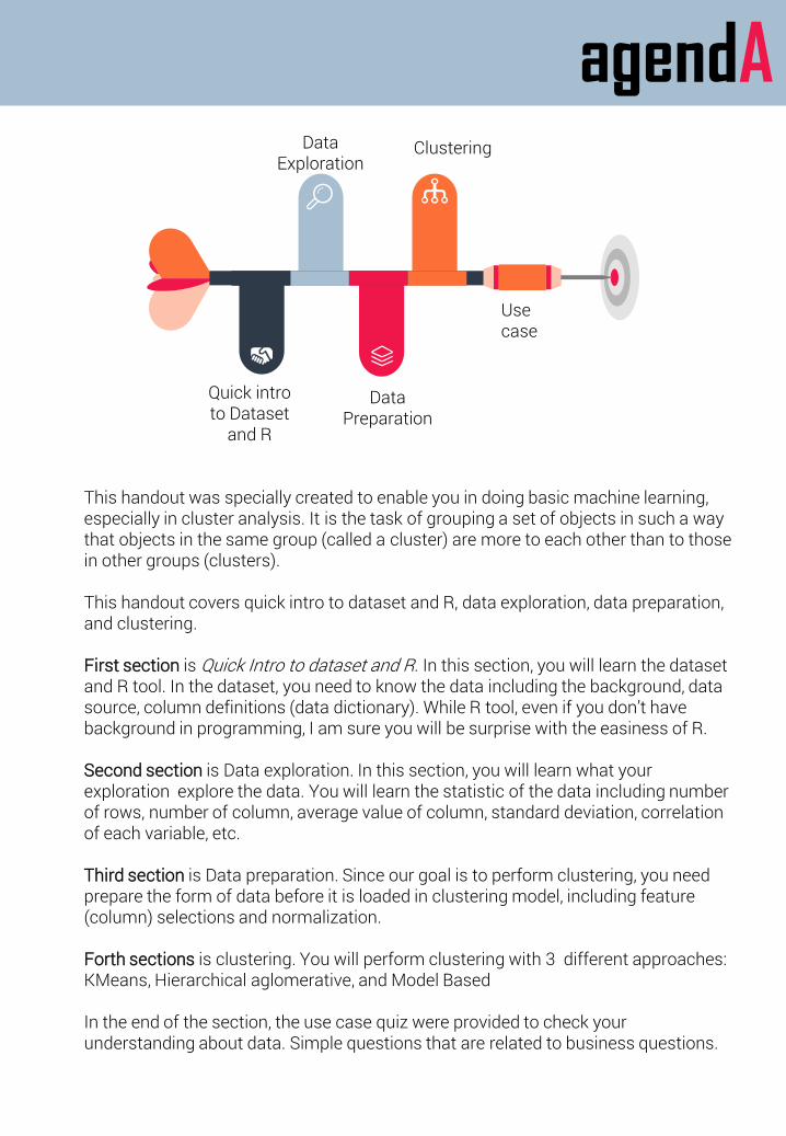
This handout was specially created to enable you in doing basic machine learning, especially in cluster analysis. It is the task of grouping a set of objects in such a way that objects in the same group (called a cluster) are more to each other than to those in other groups (clusters).

This handout covers quick intro to dataset and R, data exploration, data preparation, and clustering.

First section is Quick Intro to dataset and R. In this section, you will learn the dataset and R tool. In the dataset, you need to know the data including the background, data source, column definitions (data dictionary). While R tool, even if you don’t have background in programming, I am sure you will be surprise with the easiness of R.

Second section is Data exploration. In this section, you will learn what your exploration explore the data. You will learn the statistic of the data including number of rows, number of column, average value of column, standard deviation, correlation of each variable, etc.

Third section is Data preparation. Since our goal is to perform clustering, you need prepare the form of data before it is loaded in clustering model, including feature (column) selections and normalization.

Forth sections is clustering. You will perform clustering with 3 different approaches: KMeans, Hierarchical aglomerative, and Model Based

In the end of the section, the use case quiz were provided to check your understanding about data. Simple questions that are related to business questions.

Typical ProjecT

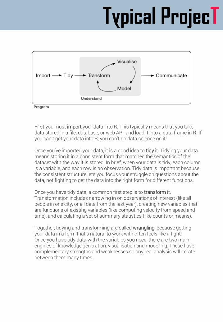
First you must import your data into R. This typically means that you take data stored in a file, database, or web API, and load it into a data frame in R. If you can’t get your data into R, you can’t do data science on it!

Once you’ve imported your data, it is a good idea to tidy it. Tidying your data means storing it in a consistent form that matches the semantics of the dataset with the way it is stored. In brief, when your data is tidy, each column is a variable, and each row is an observation. Tidy data is important because the consistent structure lets you focus your struggle on questions about the data, not fighting to get the data into the right form for different functions.

Once you have tidy data, a common first step is to transform it. Transformation includes narrowing in on observations of interest (like all people in one city, or all data from the last year), creating new variables that are functions of existing variables (like computing velocity from speed and time), and calculating a set of summary statistics (like counts or means).

Together, tidying and transforming are called wrangling, because getting your data in a form that’s natural to work with often feels like a fight!Once you have tidy data with the variables you need, there are two main engines of knowledge generation: visualisation and modelling. These have complementary strengths and weaknesses so any real analysis will iterate between them many times.

Part 1Quick intro to the dataset and R

dataseT

World Happiness Record https://www.kaggle.com/unsdsn/world-happiness

Download

ContextThe World Happiness Report is a landmark survey of the state of globalhappiness. The first report was published in 2012, the second in 2013, the thirdin 2015, and the fourth in the 2016 Update. The World Happiness 2017, whichranks 155 countries by their happiness levels, was released at the UnitedNations at an event celebrating International Day of Happiness on March 20th.The report continues to gain global recognition as governments, organizationsand civil society increasingly use happiness indicators to inform their policy-making decisions. Leading experts across fields – economics, psychology,survey analysis, national statistics, health, public policy and more – describehow measurements of well-being can be used effectively to assess the progressof nations. The reports review the state of happiness in the world today andshow how the new science of happiness explains personal and nationalvariations in happiness.

ContentThe happiness scores and rankings use data from the Gallup World Poll. Thescores are based on answers to the main life evaluation question asked in thepoll. This question, known as the Cantril ladder, asks respondents to think of aladder with the best possible life for them being a 10 and the worst possible lifebeing a 0 and to rate their own current lives on that scale. The scores are fromnationally representative samples for the years 2013-2016 and use the Gallupweights to make the estimates representative. The columns following thehappiness score estimate the extent to which each of six factors – economicproduction, social support, life expectancy, freedom, absence of corruption, andgenerosity – contribute to making life evaluations higher in each country thanthey are in Dystopia, a hypothetical country that has values equal to the world’slowest national averages for each of the six factors. They have no impact on thetotal score reported for each country, but they do explain why some countriesrank higher than others.

dataseT

What is Dystopia?Dystopia is an imaginary country that has the world’s least-happy people. The purpose in establishing Dystopia is to have a benchmark against which all countries can be favorably compared (no country performs more poorly than Dystopia) in terms of each of the six key variables, thus allowing each sub-bar to be of positive width. The lowest scores observed for the six key variables, therefore, characterize Dystopia. Since life would be very unpleasant in a country with the world’s lowest incomes, lowest life expectancy, lowest generosity, most corruption, least freedom and least social support, it is referred to as “Dystopia,” in contrast to Utopia.

What are the residuals?The residuals, or unexplained components, differ for each country, reflecting the extent to which the six variables either over- or under-explain average 2014-2016 life evaluations. These residuals have an average value of approximately zero over the whole set of countries. Figure 2.2 shows the average residual for each country when the equation in Table 2.1 is applied to average 2014- 2016 data for the six variables in that country. We combine these residuals with the estimate for life evaluations in Dystopia so that the combined bar will always have positive values. As can be seen in Figure 2.2, although some life evaluation residuals are quite large, occasionally exceeding one point on the scale from 0 to 10, they are always much smaller than the calculated value in Dystopia, where the average life is rated at 1.85 on the 0 to 10 scale.

What do the columns succeeding the Happiness Score(like Family, Generosity, etc.) describe?The following columns: GDP per Capita, Family, Life Expectancy, Freedom, Generosity, Trust Government Corruption describe the extent to which these factors contribute in evaluating the happiness in each country. The Dystopia Residual metric actually is the Dystopia Happiness Score(1.85) + the Residual value or the unexplained value for each country as stated in the previous answer.If you add all these factors up, you get the happiness score so it might be un-reliable to model them to predict Happiness Scores.

Quick intro to R

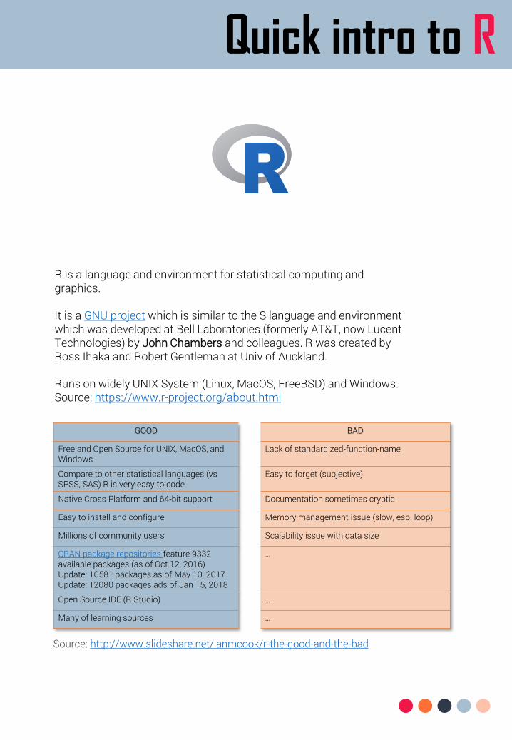
R is a language and environment for statistical computing and graphics.

It is a GNU project which is similar to the S language and environment which was developed at Bell Laboratories (formerly AT&T, now Lucent Technologies) by John Chambers and colleagues. R was created by Ross Ihaka and Robert Gentleman at Univ of Auckland.

Runs on widely UNIX System (Linux, MacOS, FreeBSD) and Windows.Source: https://www.r-project.org/about.html

GOOD BAD

Free and Open Source for UNIX, MacOS, and Windows

Lack of standardized-function-name

Compare to other statistical languages (vs SPSS, SAS) R is very easy to code

Easy to forget (subjective)

Native Cross Platform and 64-bit support Documentation sometimes cryptic

Easy to install and configure Memory management issue (slow, esp. loop)

Millions of community users Scalability issue with data size

CRAN package repositories feature 9332available packages (as of Oct 12, 2016)Update: 10581 packages as of May 10, 2017Update: 12080 packages ads of Jan 15, 2018

…

Open Source IDE (R Studio) …

Many of learning sources …

Source: http://www.slideshare.net/ianmcook/r-the-good-and-the-bad

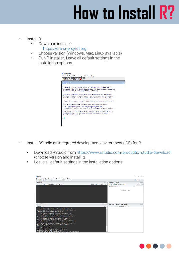
How to Install R?

• Install R • Download installer

https://cran.r-project.org• Choose version (Windows, Mac, Linux available)• Run R installer. Leave all default settings in the

installation options.

• Install RStudio as integrated development environment (IDE) for R

• Download RStudio from https://www.rstudio.com/products/rstudio/download(choose version and install it)

• Leave all default settings in the installation options

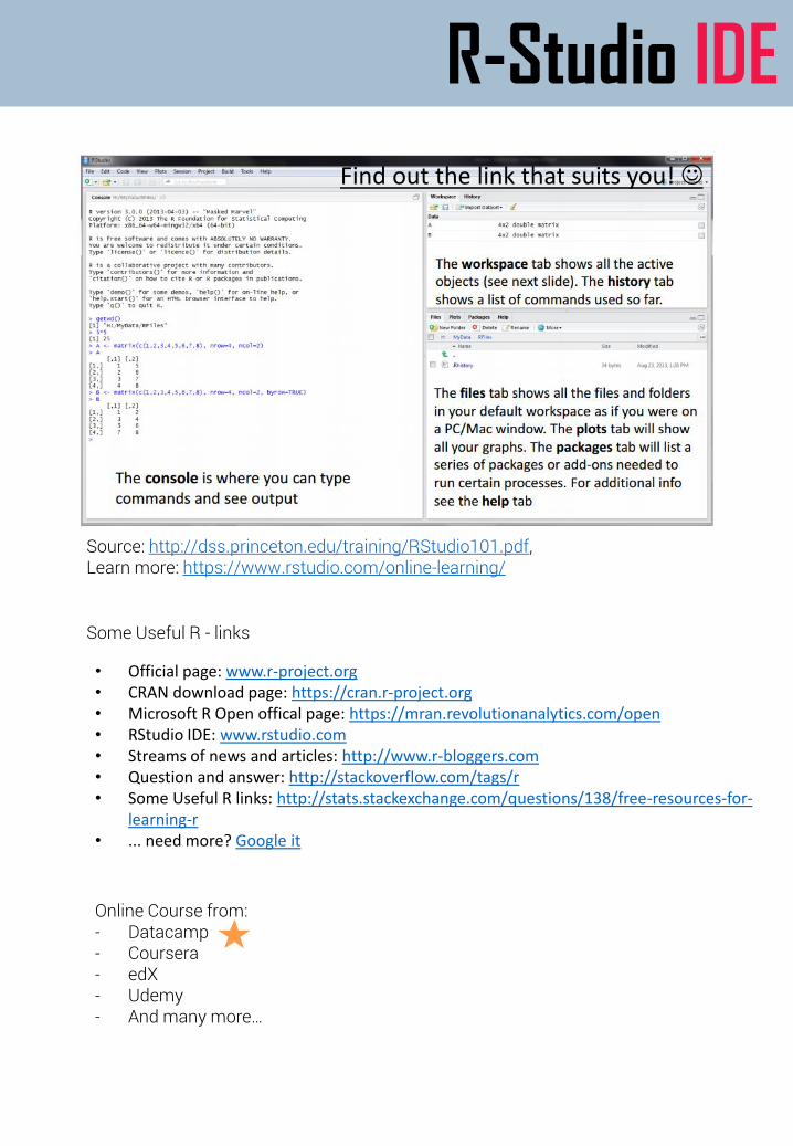
R-Studio IDE

Source: http://dss.princeton.edu/training/RStudio101.pdf,Learn more: https://www.rstudio.com/online-learning/

Some Useful R - links

Find out the link that suits you! ☺

• Official page: www.r-project.org• CRAN download page: https://cran.r-project.org• Microsoft R Open offical page: https://mran.revolutionanalytics.com/open• RStudio IDE: www.rstudio.com• Streams of news and articles: http://www.r-bloggers.com• Question and answer: http://stackoverflow.com/tags/r• Some Useful R links: http://stats.stackexchange.com/questions/138/free-resources-for-

learning-r• ... need more? Google it

Online Course from:- Datacamp- Coursera - edX- Udemy- And many more…

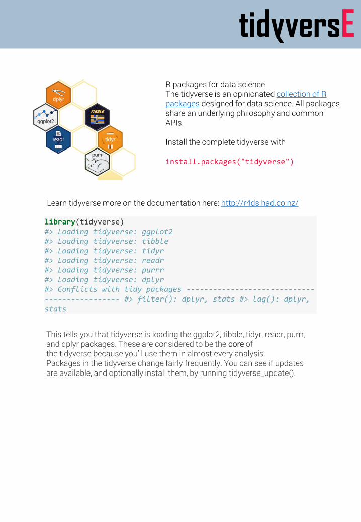
tidyversE

R packages for data scienceThe tidyverse is an opinionated collection of R packages designed for data science. All packages share an underlying philosophy and common APIs.

Install the complete tidyverse with

install.packages("tidyverse")

Learn tidyverse more on the documentation here: http://r4ds.had.co.nz/

library(tidyverse) #> Loading tidyverse: ggplot2#> Loading tidyverse: tibble#> Loading tidyverse: tidyr#> Loading tidyverse: readr#> Loading tidyverse: purrr#> Loading tidyverse: dplyr#> Conflicts with tidy packages ---------------------------------------------- #> filter(): dplyr, stats #> lag(): dplyr, stats

This tells you that tidyverse is loading the ggplot2, tibble, tidyr, readr, purrr, and dplyr packages. These are considered to be the core of the tidyverse because you’ll use them in almost every analysis.Packages in the tidyverse change fairly frequently. You can see if updates are available, and optionally install them, by running tidyverse_update().

Part 2Data Exploration

explorE

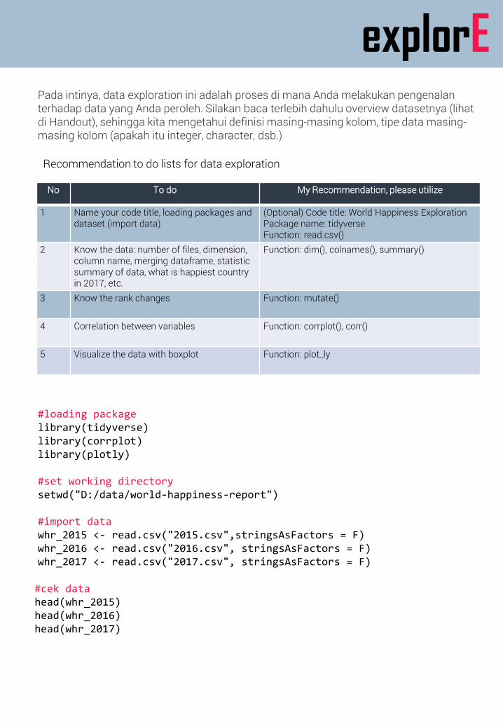
No To do My Recommendation, please utilize

1 Name your code title, loading packages and dataset (import data)

(Optional) Code title: World Happiness ExplorationPackage name: tidyverseFunction: read.csv()

2 Know the data: number of files, dimension, column name, merging dataframe, statistic summary of data, what is happiest country in 2017, etc.

Function: dim(), colnames(), summary()

3 Know the rank changes Function: mutate()

4 Correlation between variables Function: corrplot(), corr()

5 Visualize the data with boxplot Function: plot_ly

#loading packagelibrary(tidyverse)library(corrplot)library(plotly)

#set working directorysetwd("D:/data/world-happiness-report")

#import datawhr_2015 <- read.csv("2015.csv",stringsAsFactors = F)whr_2016 <- read.csv("2016.csv", stringsAsFactors = F)whr_2017 <- read.csv("2017.csv", stringsAsFactors = F)

#cek datahead(whr_2015)head(whr_2016)head(whr_2017)

Pada intinya, data exploration ini adalah proses di mana Anda melakukan pengenalanterhadap data yang Anda peroleh. Silakan baca terlebih dahulu overview datasetnya (lihatdi Handout), sehingga kita mengetahui definisi masing-masing kolom, tipe data masing-masing kolom (apakah itu integer, character, dsb.)

Recommendation to do lists for data exploration

explorE

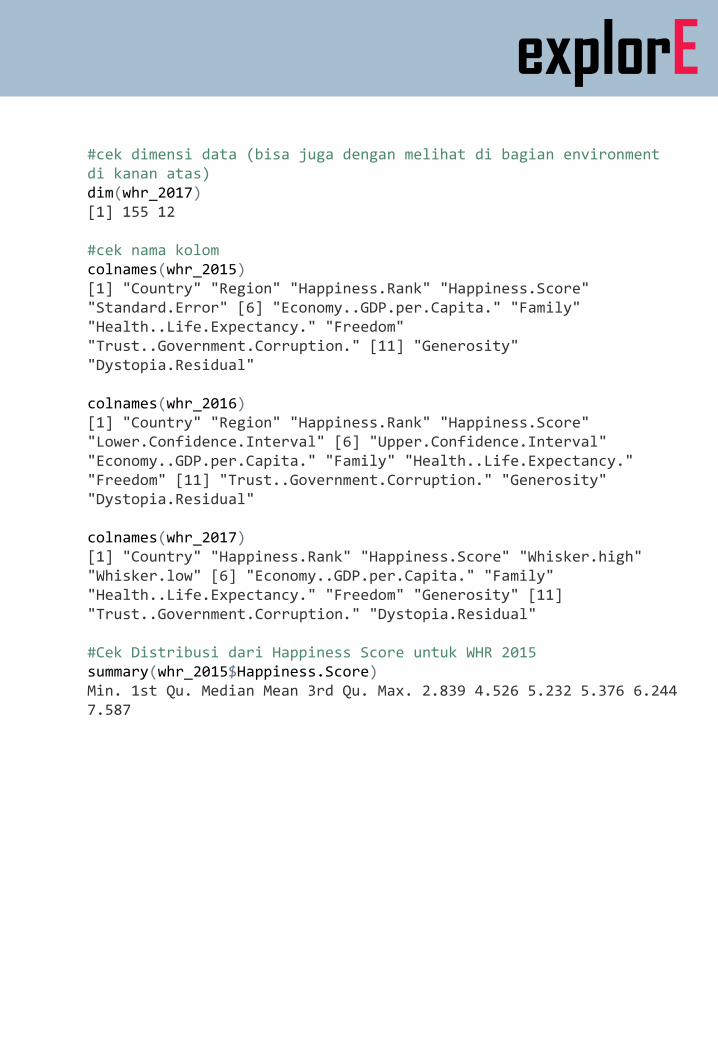
#cek dimensi data (bisa juga dengan melihat di bagian environment di kanan atas)dim(whr_2017)[1] 155 12

#cek nama kolomcolnames(whr_2015)[1] "Country" "Region" "Happiness.Rank" "Happiness.Score" "Standard.Error" [6] "Economy..GDP.per.Capita." "Family" "Health..Life.Expectancy." "Freedom" "Trust..Government.Corruption." [11] "Generosity" "Dystopia.Residual"

colnames(whr_2016)[1] "Country" "Region" "Happiness.Rank" "Happiness.Score" "Lower.Confidence.Interval" [6] "Upper.Confidence.Interval" "Economy..GDP.per.Capita." "Family" "Health..Life.Expectancy." "Freedom" [11] "Trust..Government.Corruption." "Generosity" "Dystopia.Residual"

colnames(whr_2017)[1] "Country" "Happiness.Rank" "Happiness.Score" "Whisker.high" "Whisker.low" [6] "Economy..GDP.per.Capita." "Family" "Health..Life.Expectancy." "Freedom" "Generosity" [11] "Trust..Government.Corruption." "Dystopia.Residual"

#Cek Distribusi dari Happiness Score untuk WHR 2015summary(whr_2015$Happiness.Score)Min. 1st Qu. Median Mean 3rd Qu. Max. 2.839 4.526 5.232 5.376 6.244 7.587

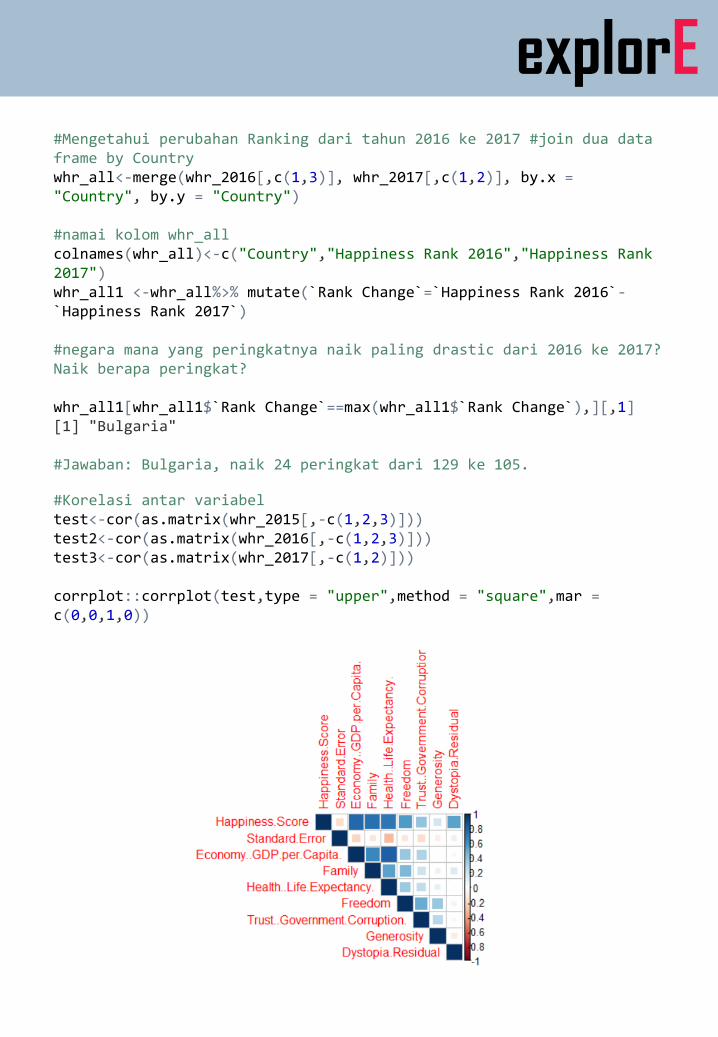
explorE#Mengetahui perubahan Ranking dari tahun 2016 ke 2017 #join dua data frame by Countrywhr_all<-merge(whr_2016[,c(1,3)], whr_2017[,c(1,2)], by.x ="Country", by.y = "Country")

#namai kolom whr_allcolnames(whr_all)<-c("Country","Happiness Rank 2016","Happiness Rank 2017")whr_all1 <-whr_all%>% mutate(`Rank Change`=`Happiness Rank 2016`-`Happiness Rank 2017`)

#negara mana yang peringkatnya naik paling drastic dari 2016 ke 2017? Naik berapa peringkat?

whr_all1[whr_all1$`Rank Change`==max(whr_all1$`Rank Change`),][,1][1] "Bulgaria"

#Jawaban: Bulgaria, naik 24 peringkat dari 129 ke 105.

#Korelasi antar variabeltest<-cor(as.matrix(whr_2015[,-c(1,2,3)]))test2<-cor(as.matrix(whr_2016[,-c(1,2,3)]))test3<-cor(as.matrix(whr_2017[,-c(1,2)]))

corrplot::corrplot(test,type = "upper",method = "square",mar =c(0,0,1,0))

Part 3Data Preparation

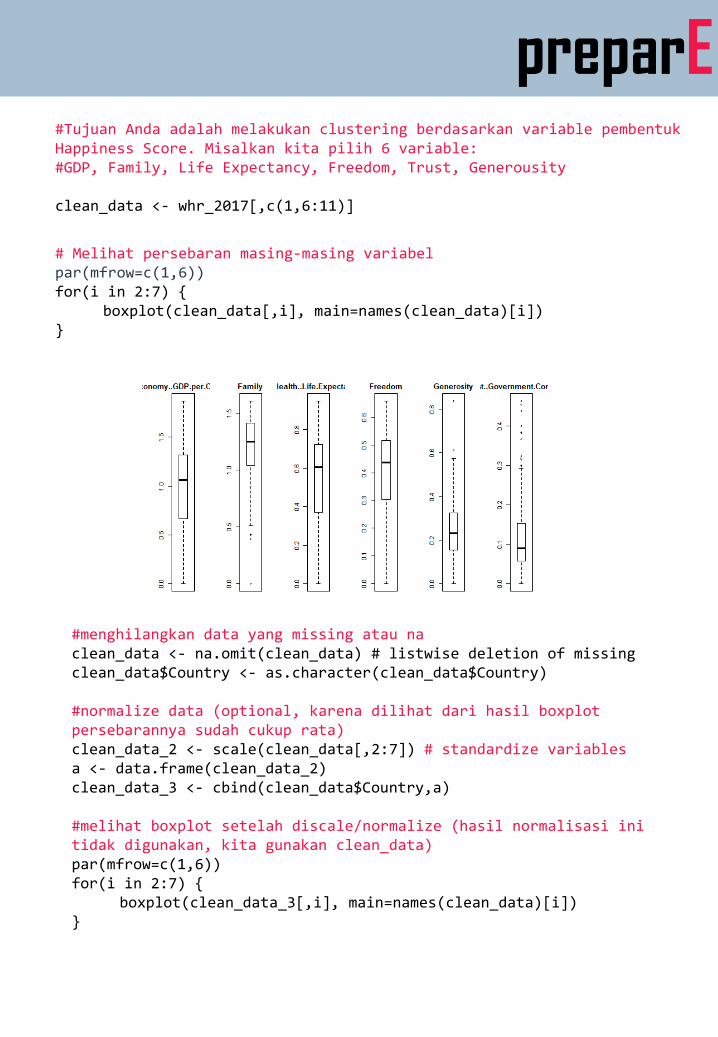
preparE#Tujuan Anda adalah melakukan clustering berdasarkan variable pembentukHappiness Score. Misalkan kita pilih 6 variable:#GDP, Family, Life Expectancy, Freedom, Trust, Generousity

clean_data <- whr_2017[,c(1,6:11)]

# Melihat persebaran masing-masing variabelpar(mfrow=c(1,6))for(i in 2:7) {

boxplot(clean_data[,i], main=names(clean_data)[i])}

#menghilangkan data yang missing atau naclean_data <- na.omit(clean_data) # listwise deletion of missingclean_data$Country <- as.character(clean_data$Country)

#normalize data (optional, karena dilihat dari hasil boxplot persebarannya sudah cukup rata)clean_data_2 <- scale(clean_data[,2:7]) # standardize variablesa <- data.frame(clean_data_2)clean_data_3 <- cbind(clean_data$Country,a)

#melihat boxplot setelah discale/normalize (hasil normalisasi initidak digunakan, kita gunakan clean_data)par(mfrow=c(1,6))for(i in 2:7) {

boxplot(clean_data_3[,i], main=names(clean_data)[i])}

Part 4Clustering

clusterinG

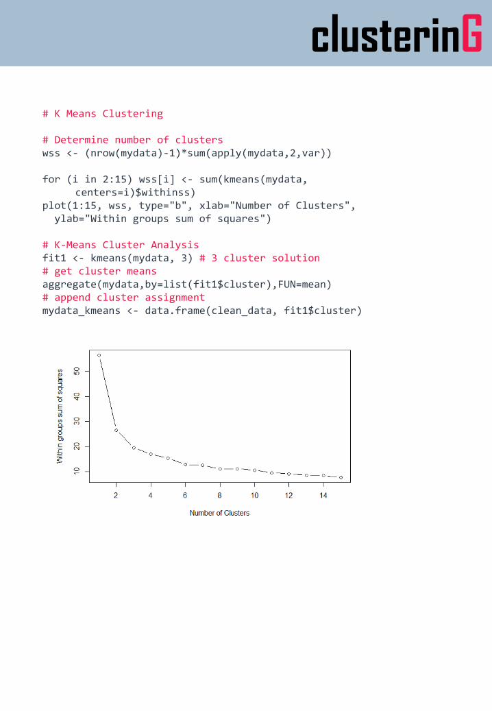
# K Means Clustering

# Determine number of clusterswss <- (nrow(mydata)-1)*sum(apply(mydata,2,var))

for (i in 2:15) wss[i] <- sum(kmeans(mydata, centers=i)$withinss)

plot(1:15, wss, type="b", xlab="Number of Clusters",ylab="Within groups sum of squares")

# K-Means Cluster Analysisfit1 <- kmeans(mydata, 3) # 3 cluster solution# get cluster means aggregate(mydata,by=list(fit1$cluster),FUN=mean)# append cluster assignmentmydata_kmeans <- data.frame(clean_data, fit1$cluster)

clusterinG

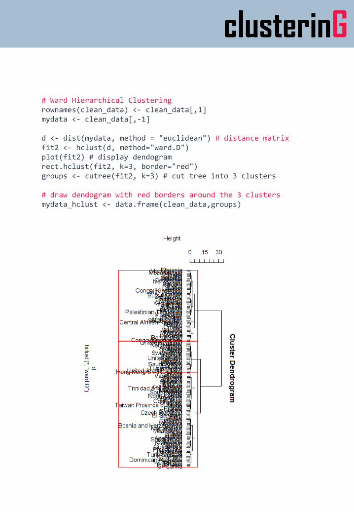
# Ward Hierarchical Clusteringrownames(clean_data) <- clean_data[,1]mydata <- clean_data[,-1]

d <- dist(mydata, method = "euclidean") # distance matrixfit2 <- hclust(d, method="ward.D") plot(fit2) # display dendogramrect.hclust(fit2, k=3, border="red")groups <- cutree(fit2, k=3) # cut tree into 3 clusters

# draw dendogram with red borders around the 3 clusters mydata_hclust <- data.frame(clean_data,groups)

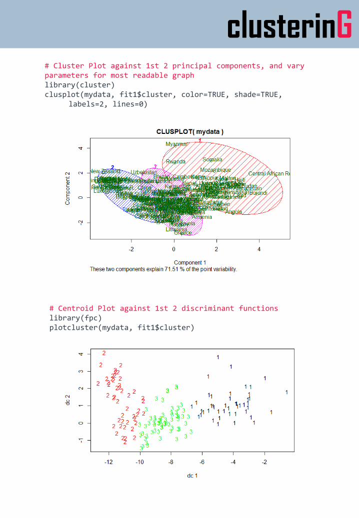
clusterinG# Cluster Plot against 1st 2 principal components, and vary parameters for most readable graphlibrary(cluster) clusplot(mydata, fit1$cluster, color=TRUE, shade=TRUE,

labels=2, lines=0)

# Centroid Plot against 1st 2 discriminant functionslibrary(fpc)plotcluster(mydata, fit1$cluster)

quiZ

Will be done in class

Vacant positions: Data Insight Analytics and Data Insight Sales at Telkomsel MSIGHT.

Interested? Please send your cover letter and Linkedin profile to my email address: b_a_kuncoro@telkomsel.co.id

Thank You