Embed Size (px)
Citation preview
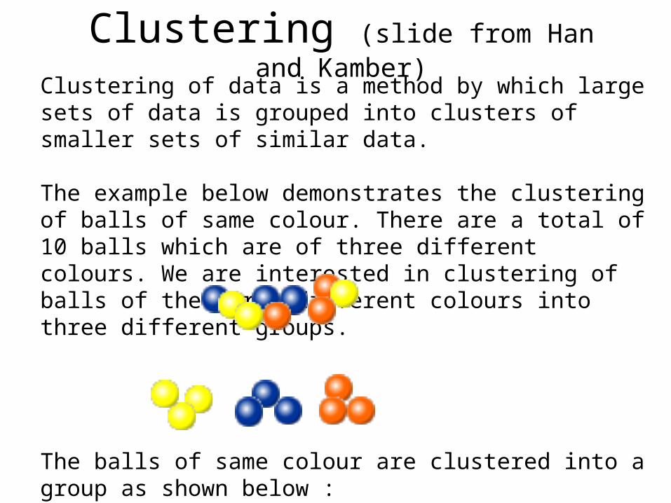
Clustering (slide from Han and Kamber)Clustering of data is a method by which large sets of data is grouped into clusters of smaller sets of similar data.
The example below demonstrates the clustering of balls of same colour. There are a total of 10 balls which are of three differentcolours. We are interested in clustering of balls of the three different colours into three different groups.
The balls of same colour are clustered into a group as shown below :
Thus, we see clustering means grouping of data or dividing a large data set into smaller data sets of some similarity.
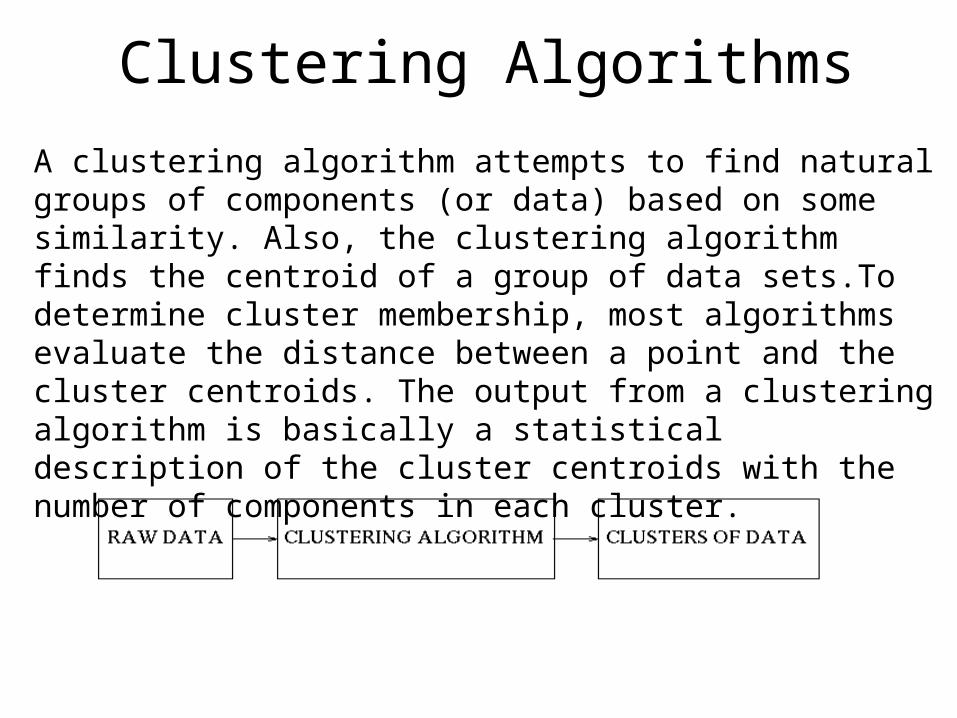
Clustering Algorithms
A clustering algorithm attempts to find natural groups of components (or data) based on some similarity. Also, the clustering algorithm finds the centroid of a group of data sets.To determine cluster membership, most algorithms evaluate the distance between a point and the cluster centroids. The output from a clustering algorithm is basically a statistical description of the cluster centroids with the number of components in each cluster.
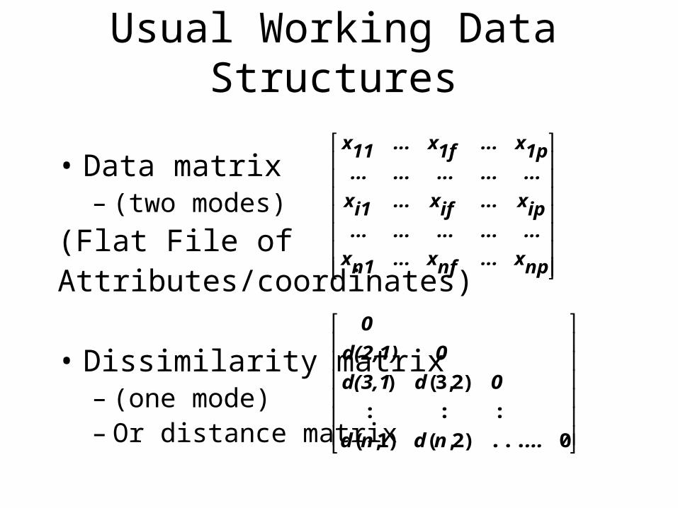
Usual Working Data Structures
• Data matrix– (two modes)
(Flat File of Attributes/coordinates)
• Dissimilarity matrix– (one mode)– Or distance matrix
npx...nfx...n1x
...............ipx...ifx...i1x
...............1px...1fx...11x
0...)2,()1,(
:::
)2,3()
...ndnd
0dd(3,1
0d(2,1)
0
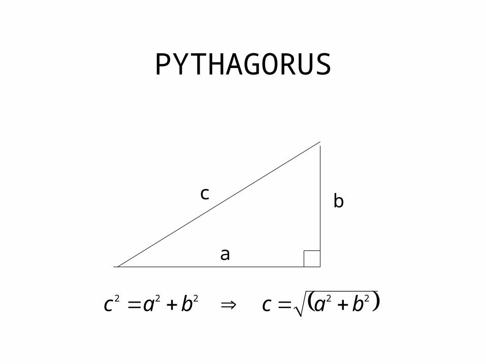
PYTHAGORUS
a
bc
22222 bacbac
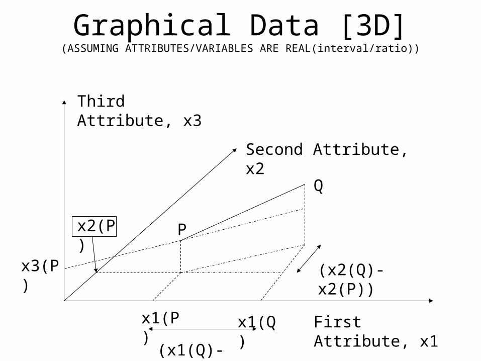
Graphical Data [3D](ASSUMING ATTRIBUTES/VARIABLES ARE REAL(interval/ratio))
First Attribute, x1
Second Attribute, x2
Third Attribute, x3
P
Q
x1(P)
x3(P)
x2(P)
x1(Q)
(x1(Q)-x1(P))
(x2(Q)-x2(P))
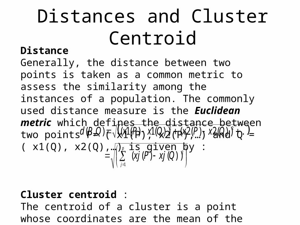
Distances and Cluster CentroidDistanceGenerally, the distance between two points is taken as a common metric to assess the similarity among the instances of a population. The commonly used distance measure is the Euclidean metric which defines the distance between two points P= ( x1(P), x2(P),…) and Q = ( x1(Q), x2(Q),…) is given by :
Cluster centroid :The centroid of a cluster is a point whose coordinates are the mean of the coordinates of all the points in the clusters.
2
1
22
))()((
...))(2)(2())(1)(1(),(
QxjPxj
QxPxQxPxQPd
p
j
Distance-based Clustering
• Define/Adopt distance measure data instances• Find a partition of the instances such that:
– Distance between objects within partition (i.e. same cluster) is minimized
– Distance between objects from different clusters is maximised
• Issues :– Requires defining a distance (similarity) measure in situation
where it is unclear how to assign it– What relative weighting to give to one attribute vs another?– Number of possible partition is super-exponential in n.
Generalized Distances, and Similarity Measures
• The distance metric is a Dissimilarity measure.• Two points are “similar” if they are “close”, or dist is near 0.• Hence Similarity can be expressed in terms of a distance
function. For example:s(P,Q) = 1 / ( 1 + d(P,Q) )
• The definitions of distance functions are usually very different for interval-scaled, boolean, categorical, ordinal and ratio variables.
• Weights should be associated with different coordinate dimensions, based on applications and data semantics.
• It is hard to define “similar enough” or “good enough” – the answer is typically highly subjective.
Type of data in clustering analysis• Interval-scaled variables:
• Binary variables:
• Nominal, ordinal, and ratio variables:
• Variables of mixed types:
• Note: The following seven slides are optional. They are given to fill in
some of the background which is missed in R & G, because they do not
wish to reveal their instance similarity measure, for commercial reasons.
Understanding these slides really depends on some mathematical
background.
Real/Interval-valued variables
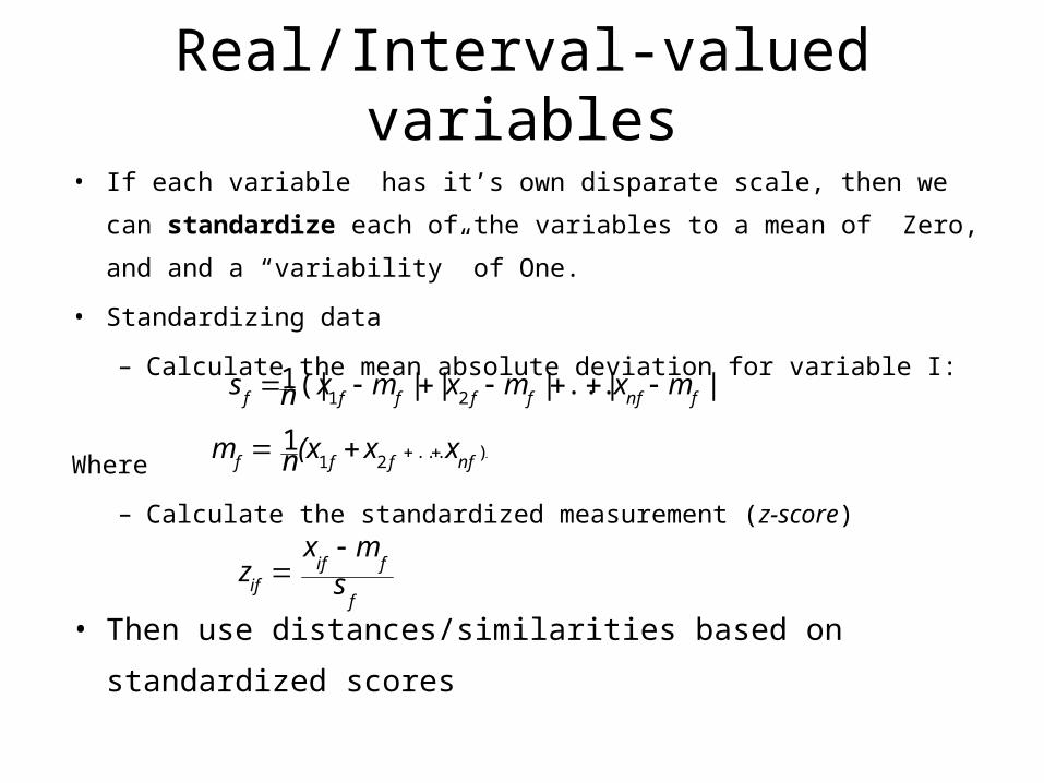
• If each variable has it’s own disparate scale, then we can standardize each
of the variables to a mean of Zero, and and a “variability” of One.
• Standardizing data
– Calculate the mean absolute deviation for variable I:
Where
– Calculate the standardized measurement (z-score)
• Then use distances/similarities based on standardized scores
.)...21
1nffff
xx(xn m
|)|...|||(|121 fnffffff
mxmxmxns
f
fifif s
mx z
Generalized Distances Between Objects
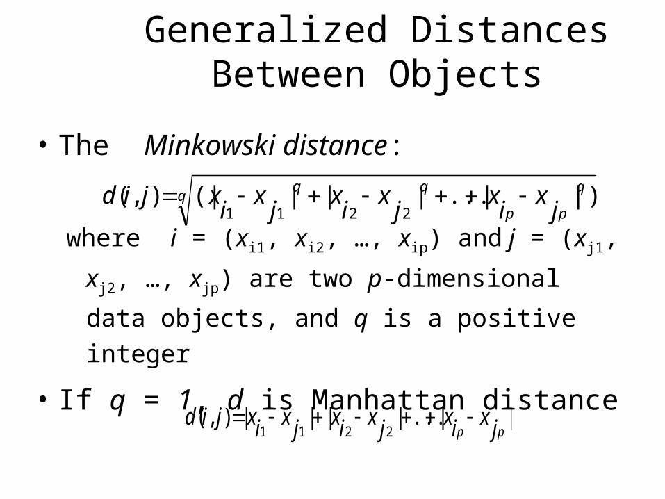
• The Minkowski distance:
where i = (xi1, xi2, …, xip) and j = (xj1, xj2, …, xjp) are
two p-dimensional data objects, and q is a positive
integer
• If q = 1, d is Manhattan distance
pp
jx
ix
jx
ix
jx
ixjid )||...|||(|),(
2211
||...||||),(2211 pp jxixjxixjxixjid
Binary Variables
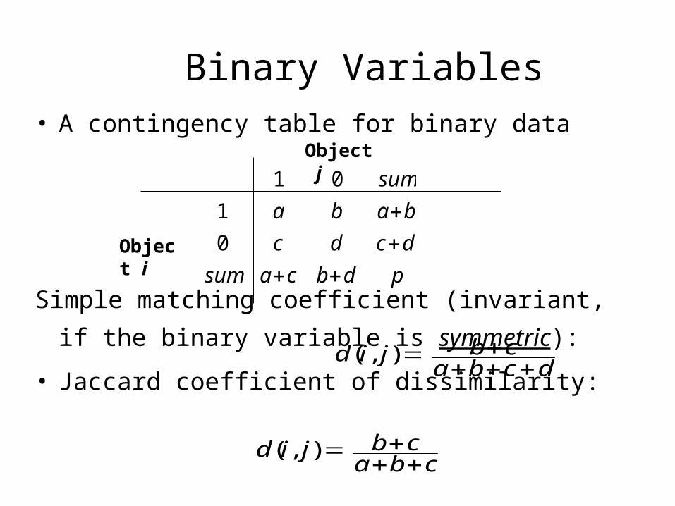
• A contingency table for binary data
Simple matching coefficient (invariant, if the binary
variable is symmetric):
• Jaccard coefficient of dissimilarity: dcba
cb jid
),(
pdbcasum
dcdc
baba
sum
0
1
01
cbacb jid
),(
Object i
Object j
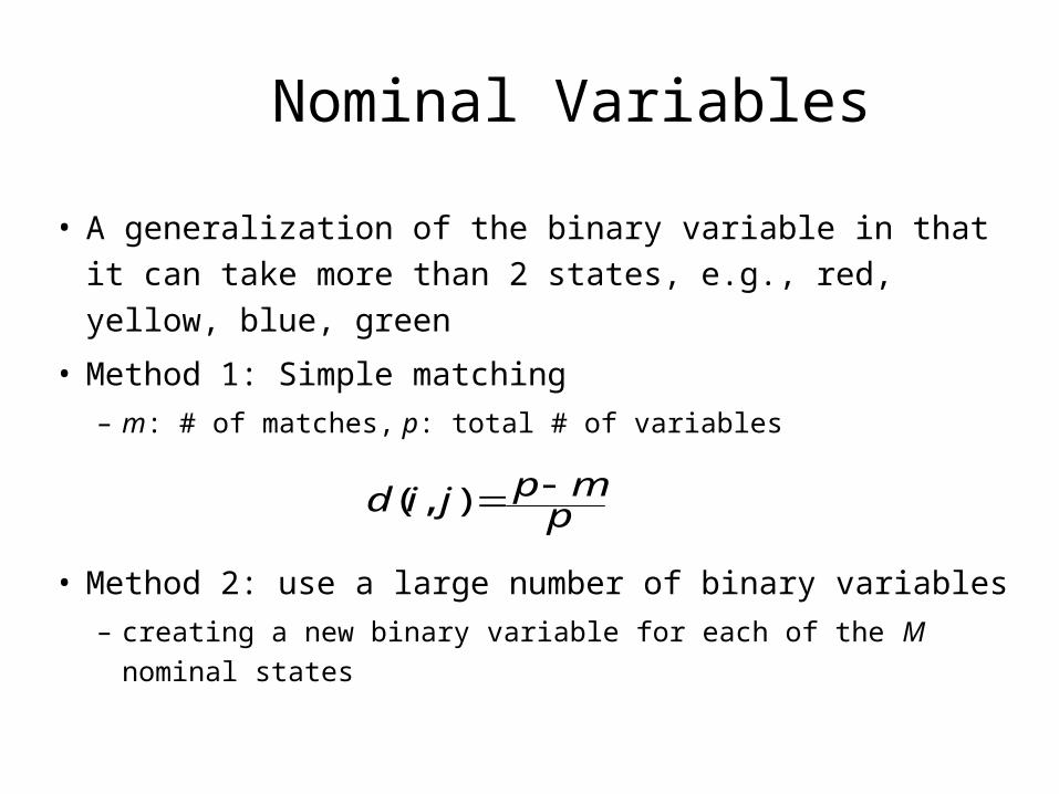
Nominal Variables
• A generalization of the binary variable in that it can take
more than 2 states, e.g., red, yellow, blue, green
• Method 1: Simple matching
– m: # of matches, p: total # of variables
• Method 2: use a large number of binary variables
– creating a new binary variable for each of the M nominal states
pmpjid ),(
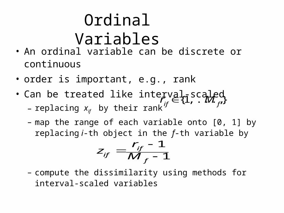
Ordinal Variables• An ordinal variable can be discrete or continuous
• order is important, e.g., rank
• Can be treated like interval-scaled
– replacing xif by their rank
– map the range of each variable onto [0, 1] by replacing i-th object in the f-th variable by
– compute the dissimilarity using methods for interval-scaled variables
11
f
ifif M
rz
},...,1{fif
Mr
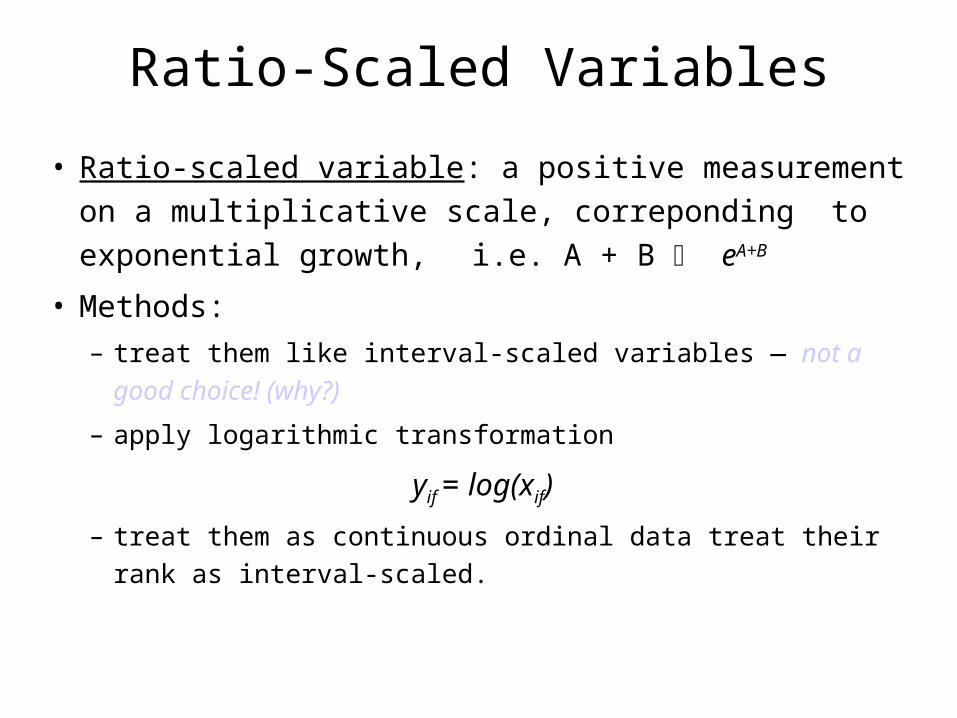
Ratio-Scaled Variables
• Ratio-scaled variable: a positive measurement on a
multiplicative scale, correponding to exponential growth,
i.e. A + B eA+B
• Methods:
– treat them like interval-scaled variables — not a good choice!
(why?)
– apply logarithmic transformation
yif = log(xif)
– treat them as continuous ordinal data treat their rank as interval-
scaled.
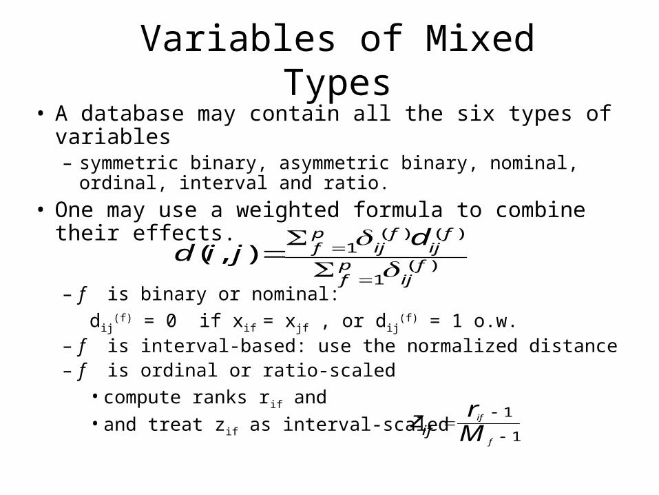
Variables of Mixed Types• A database may contain all the six types of variables
– symmetric binary, asymmetric binary, nominal, ordinal, interval and ratio.
• One may use a weighted formula to combine their effects.
– f is binary or nominal:
dij(f) = 0 if xif = xjf , or dij
(f) = 1 o.w.– f is interval-based: use the normalized distance– f is ordinal or ratio-scaled
• compute ranks rif and • and treat zif as interval-scaled
)(1
)()(1),(
fij
pf
fij
fij
pf
djid
1
1
f
if
Mrz
if
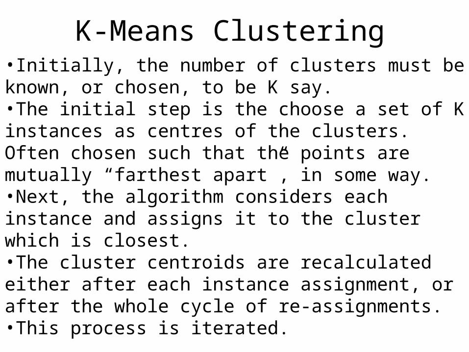
K-Means Clustering •Initially, the number of clusters must be known, or chosen, to be K say. •The initial step is the choose a set of K instances as centres of the clusters. Often chosen such that the points are mutually “farthest apart”, in some way. •Next, the algorithm considers each instance and assigns it to the cluster which is closest.•The cluster centroids are recalculated either after each instance assignment, or after the whole cycle of re-assignments.•This process is iterated.
Other K-mean Algorithm features
• Using cluster centroid to represent cluster
•Assigning data elements to the closest cluster (centre).
•Goal: Minimise the sum of the within cluster variances
•Variations of K-Means
–Initialisation (select the number of clusters, initial partitions)
–Updating of center
–Hill-climbing (trying to move an object to another cluster).
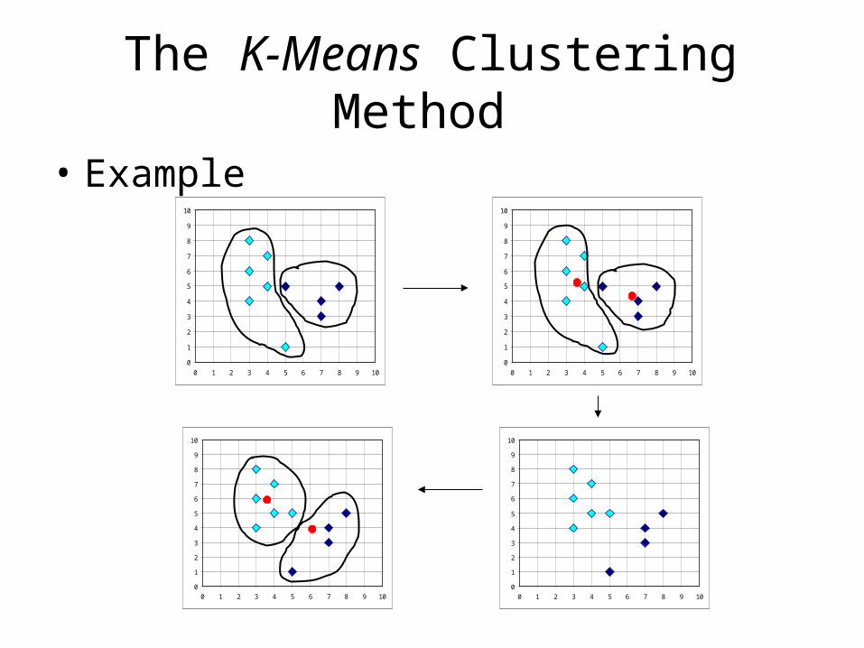
The K-Means Clustering Method
• Example
0
1
2
3
4
5
6
7
8
9
10
0 1 2 3 4 5 6 7 8 9 10
0
1
2
3
4
5
6
7
8
9
10
0 1 2 3 4 5 6 7 8 9 10
0
1
2
3
4
5
6
7
8
9
10
0 1 2 3 4 5 6 7 8 9 10
0
1
2
3
4
5
6
7
8
9
10
0 1 2 3 4 5 6 7 8 9 10
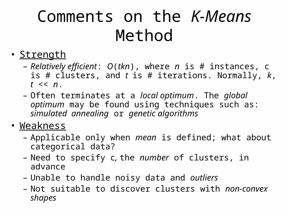
Comments on the K-Means Method
• Strength – Relatively efficient: O(tkn), where n is # instances, c is #
clusters, and t is # iterations. Normally, k, t << n.– Often terminates at a local optimum. The global optimum may
be found using techniques such as: simulated annealing or genetic algorithms
• Weakness– Applicable only when mean is defined; what about categorical
data?– Need to specify c, the number of clusters, in advance– Unable to handle noisy data and outliers– Not suitable to discover clusters with non-convex shapes
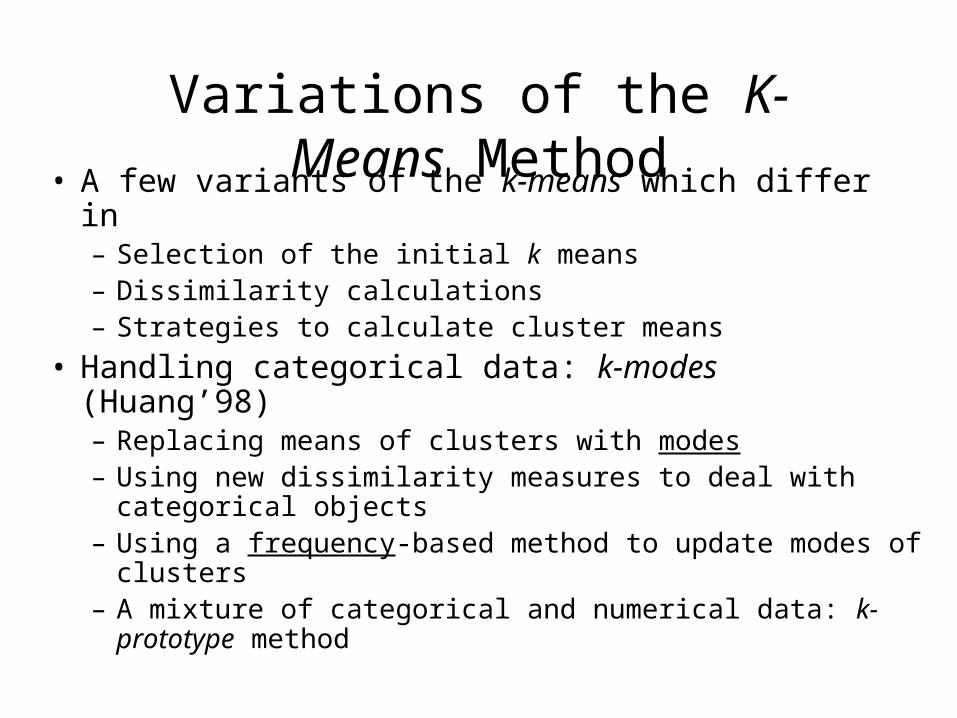
Variations of the K-Means Method• A few variants of the k-means which differ in
– Selection of the initial k means– Dissimilarity calculations– Strategies to calculate cluster means
• Handling categorical data: k-modes (Huang’98)– Replacing means of clusters with modes– Using new dissimilarity measures to deal with categorical
objects– Using a frequency-based method to update modes of clusters– A mixture of categorical and numerical data: k-prototype
method
Agglomerative Hierarchical Clustering
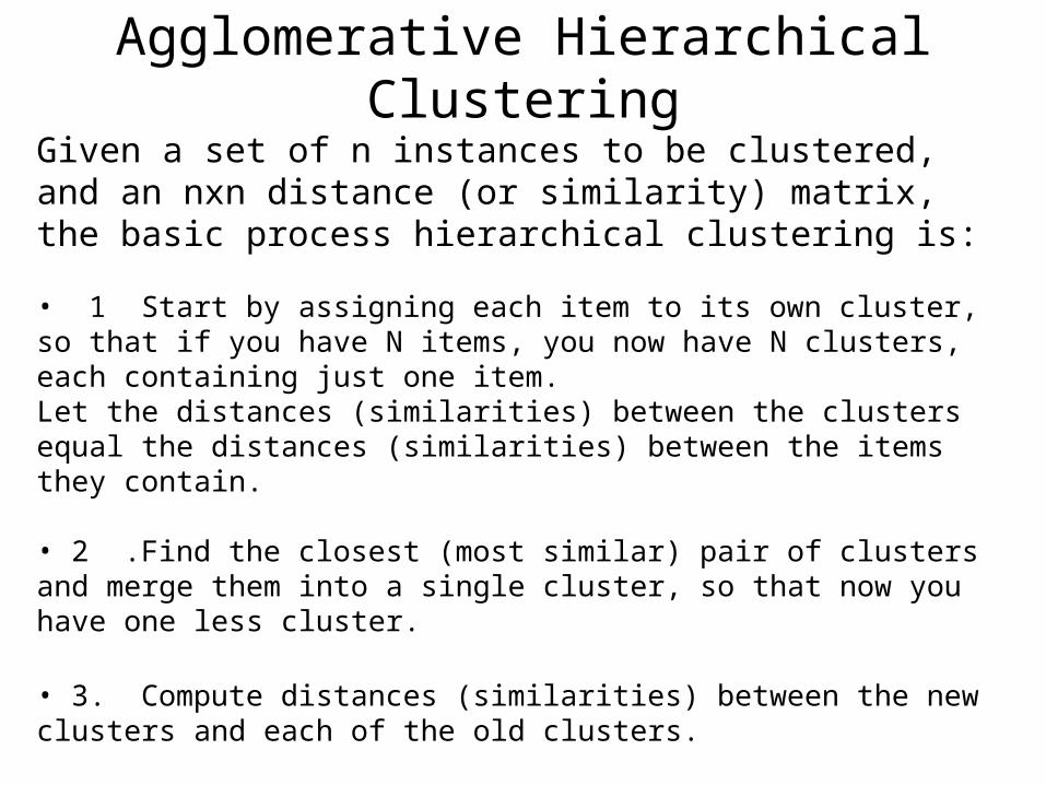
Given a set of n instances to be clustered, and an nxn distance (or similarity) matrix, the basic process hierarchical clustering is:
• 1 Start by assigning each item to its own cluster, so that if you have N items, you now have N clusters, each containing just one item. Let the distances (similarities) between the clusters equal the distances (similarities) between the items they contain.
• 2 .Find the closest (most similar) pair of clusters and merge them into a single cluster, so that now you have one less cluster.
• 3. Compute distances (similarities) between the new clusters and each of the old clusters.
• 4. Repeat steps 2 and 3 until all items are clustered into a single cluster of size n.
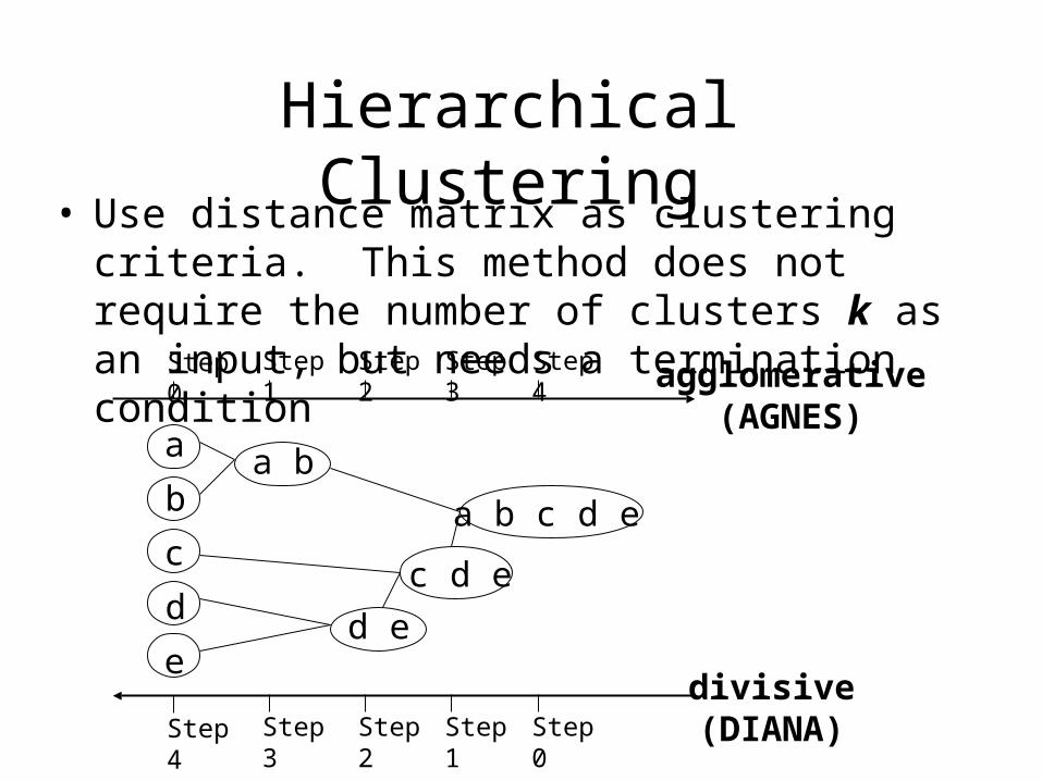
Hierarchical Clustering• Use distance matrix as clustering criteria. This
method does not require the number of clusters k as an input, but needs a termination condition
Step 0 Step 1 Step 2 Step 3 Step 4
b
d
c
e
a a b
d e
c d e
a b c d e
Step 4 Step 3 Step 2 Step 1 Step 0
agglomerative(AGNES)
divisive(DIANA)
More on Hierarchical Clustering Methods
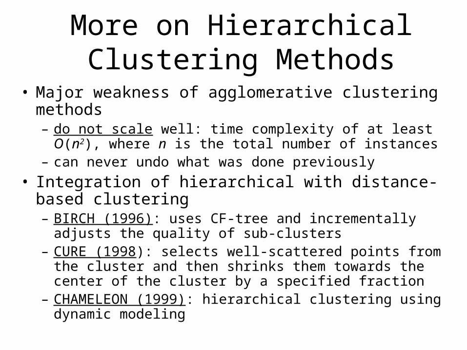
• Major weakness of agglomerative clustering methods– do not scale well: time complexity of at least O(n2), where n
is the total number of instances– can never undo what was done previously
• Integration of hierarchical with distance-based clustering– BIRCH (1996): uses CF-tree and incrementally adjusts the
quality of sub-clusters– CURE (1998): selects well-scattered points from the cluster
and then shrinks them towards the center of the cluster by a specified fraction
– CHAMELEON (1999): hierarchical clustering using dynamic modeling
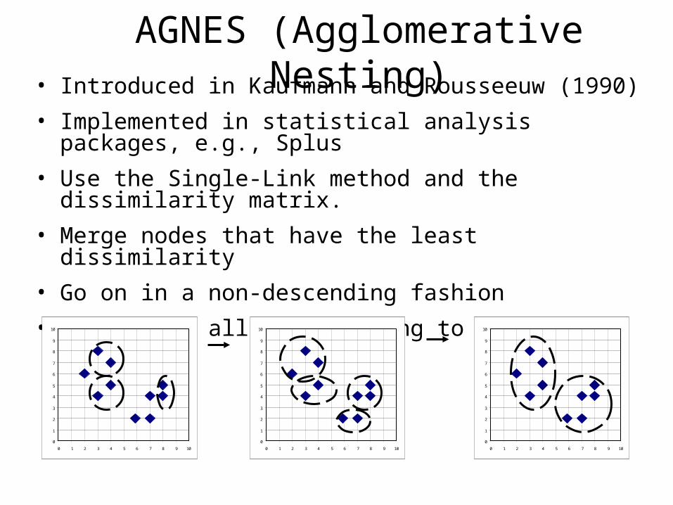
AGNES (Agglomerative Nesting)• Introduced in Kaufmann and Rousseeuw (1990)
• Implemented in statistical analysis packages, e.g., Splus
• Use the Single-Link method and the dissimilarity matrix.
• Merge nodes that have the least dissimilarity
• Go on in a non-descending fashion
• Eventually all nodes belong to the same cluster
0
1
2
3
4
5
6
7
8
9
10
0 1 2 3 4 5 6 7 8 9 10
0
1
2
3
4
5
6
7
8
9
10
0 1 2 3 4 5 6 7 8 9 10
0
1
2
3
4
5
6
7
8
9
10
0 1 2 3 4 5 6 7 8 9 10
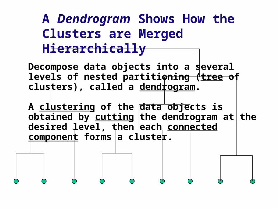
A Dendrogram Shows How the Clusters are Merged Hierarchically
Decompose data objects into a several levels of nested partitioning (tree of clusters), called a dendrogram.
A clustering of the data objects is obtained by cutting the dendrogram at the desired level, then each connected component forms a cluster.
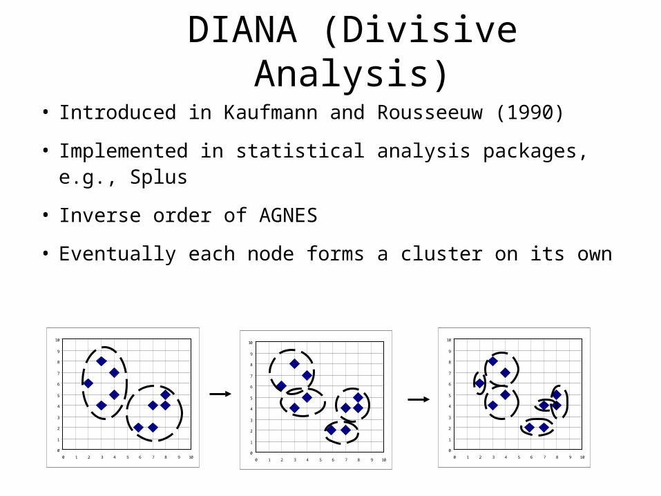
DIANA (Divisive Analysis)
• Introduced in Kaufmann and Rousseeuw (1990)
• Implemented in statistical analysis packages, e.g., Splus
• Inverse order of AGNES
• Eventually each node forms a cluster on its own
0
1
2
3
4
5
6
7
8
9
10
0 1 2 3 4 5 6 7 8 9 100
1
2
3
4
5
6
7
8
9
10
0 1 2 3 4 5 6 7 8 9 10
0
1
2
3
4
5
6
7
8
9
10
0 1 2 3 4 5 6 7 8 9 10
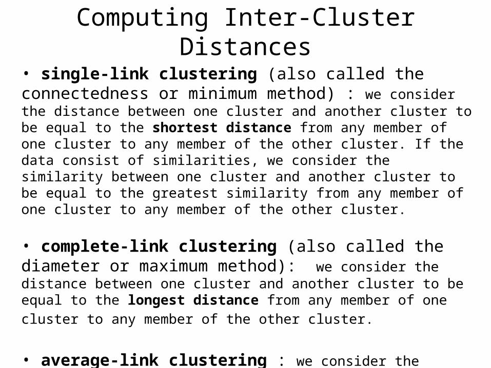
Computing Inter-Cluster Distances
• single-link clustering (also called the connectedness or minimum method) : we consider the distance between one cluster and another cluster to be equal to the shortest distance from any member of one cluster to any member of the other cluster. If the data consist of similarities, we consider the similarity between one cluster and another cluster to be equal to the greatest similarity from any member of one cluster to any member of the other cluster.
• complete-link clustering (also called the diameter or maximum method): we consider the distance between one cluster and another cluster to be equal to the longest distance from any member of one cluster to any member of
the other cluster.
• average-link clustering : we consider the distance between one cluster and another cluster to be equal to the average distance from any member of one
cluster to any member of the other cluster.
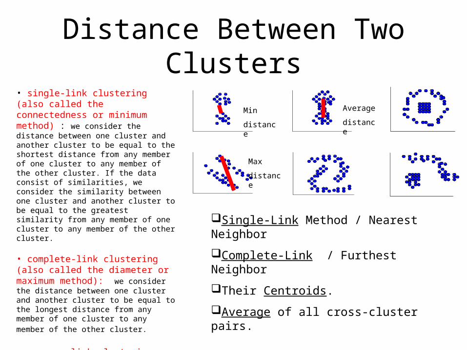
Distance Between Two Clusters
Min
distance
Average
distance
Max
distance
Single-Link Method / Nearest Neighbor
Complete-Link / Furthest Neighbor
Their Centroids.
Average of all cross-cluster pairs.
• single-link clustering (also called the connectedness or minimum method) : we consider the distance between one cluster and another cluster to be equal to the shortest distance from any member of one cluster to any member of the other cluster. If the data consist of similarities, we consider the similarity between one cluster and another cluster to be equal to the greatest similarity from any member of one cluster to any member of the other cluster.
• complete-link clustering (also called the diameter or maximum method): we consider the distance between one cluster and another cluster to be equal to the longest distance from any member of one cluster to any member of the other cluster.
• average-link clustering : we consider the distance between one cluster and another cluster to be equal to the average distance from any member of one cluster to any member of the other cluster.
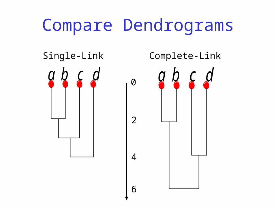
Compare Dendrograms
a b c d a b c d
2
4
6
0
Single-Link Complete-Link
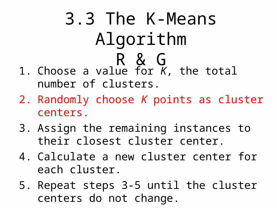
3.3 The K-Means AlgorithmR & G
1. Choose a value for K, the total number of clusters.
2. Randomly choose K points as cluster centers.
3. Assign the remaining instances to their closest cluster center.
4. Calculate a new cluster center for each cluster.
5. Repeat steps 3-5 until the cluster centers do not change.
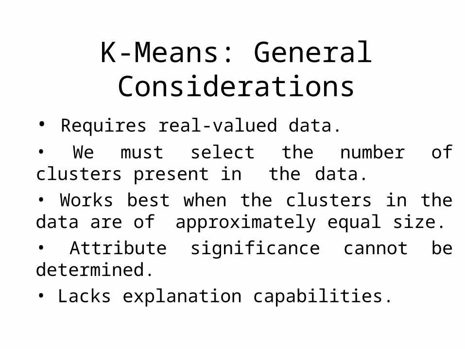
K-Means: General Considerations
• Requires real-valued data.
• We must select the number of clusters present in the data.
• Works best when the clusters in the data are of approximately equal size.• Attribute significance cannot be determined.• Lacks explanation capabilities.
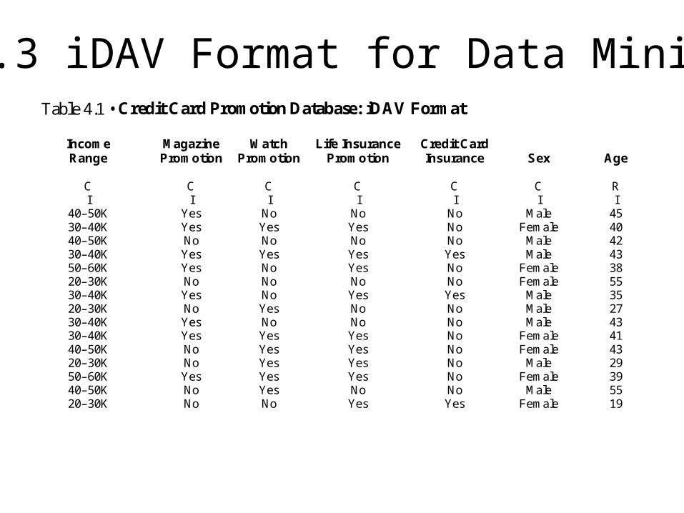
Table 4.1 • Credit Card Promotion Database: iDAV Format
Income Magazine Watch Life Insurance Credit CardRange Promotion Promotion Promotion Insurance Sex Age
C C C C C C RI I I I I I I
40–50K Yes No No No Male 4530–40K Yes Yes Yes No Female 4040–50K No No No No Male 4230–40K Yes Yes Yes Yes Male 4350–60K Yes No Yes No Female 3820–30K No No No No Female 5530–40K Yes No Yes Yes Male 3520–30K No Yes No No Male 2730–40K Yes No No No Male 4330–40K Yes Yes Yes No Female 4140–50K No Yes Yes No Female 4320–30K No Yes Yes No Male 2950–60K Yes Yes Yes No Female 3940–50K No Yes No No Male 5520–30K No No Yes Yes Female 19
4.3 iDAV Format for Data Mining
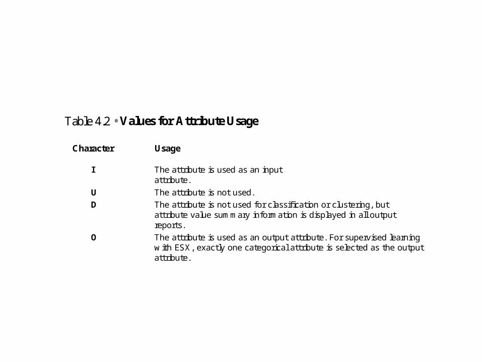
Table 4.2 • Values for Attribute Usage
Character Usage
I The attribute is used as an input attribute.
U The attribute is not used. D The attribute is not used for classification or clustering, but
attribute value summary information is displayed in all output reports.
O The attribute is used as an output attribute. For supervised learning with ESX, exactly one categorical attribute is selected as the output attribute.
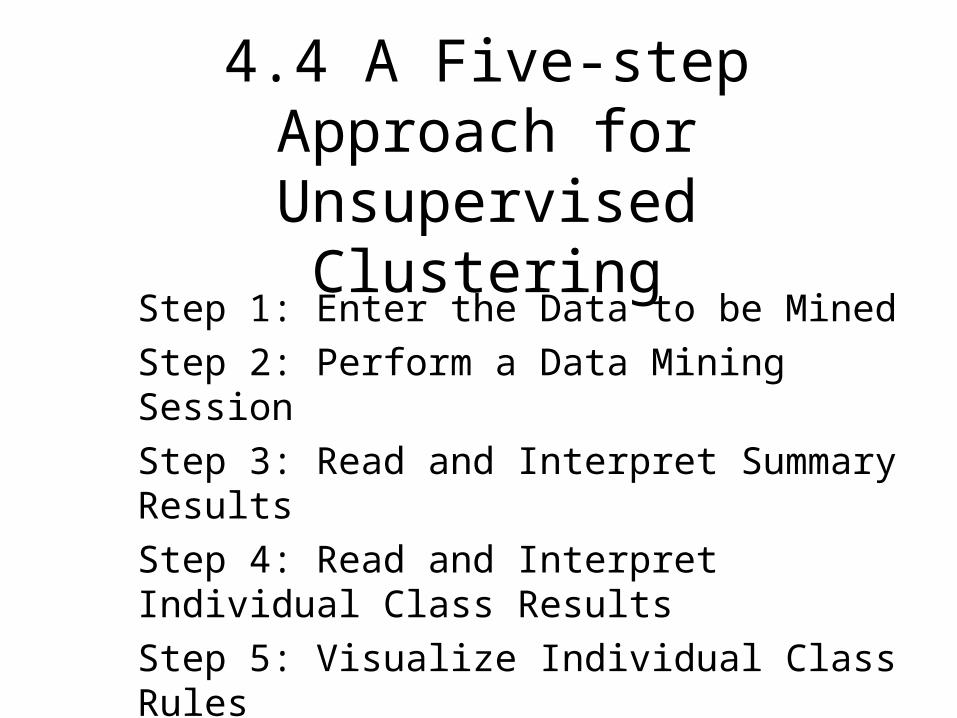
4.4 A Five-step Approach for Unsupervised Clustering
Step 1: Enter the Data to be Mined
Step 2: Perform a Data Mining Session
Step 3: Read and Interpret Summary Results
Step 4: Read and Interpret Individual Class Results
Step 5: Visualize Individual Class Rules
Step 1: Enter The Data To Be Mined
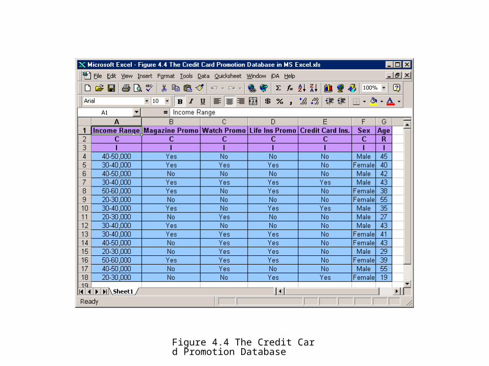
Figure 4.4 The Credit Card Promotion Database
Step 2: Perform A Data Mining Session
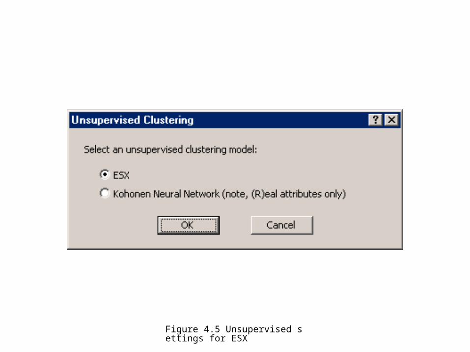
Figure 4.5 Unsupervised settings for ESX
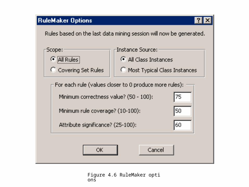
Figure 4.6 RuleMaker options
Step 3: Read and Interpret Summary Results
• Class Resemblance Scores
• Domain Resemblance Score
• Domain Predictability
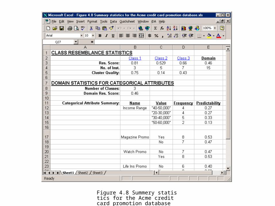
Figure 4.8 Summery statistics for the Acme credit card promotion database
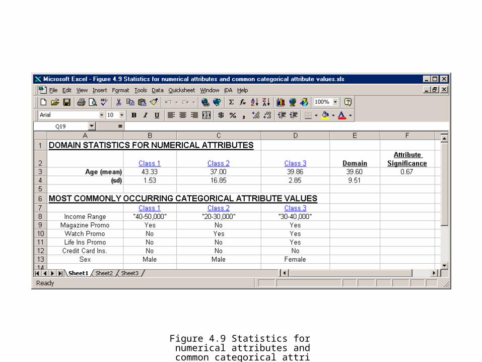
Figure 4.9 Statistics for numerical attributes and common categorical attribute values
Step 4: Read and Interpret Individual Class Results
• Class Predictability is a within-class measure.
• Class Predictiveness is a between-class measure.
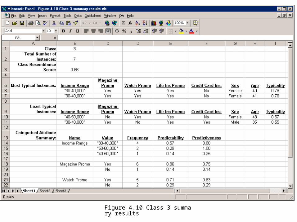
Figure 4.10 Class 3 summary results
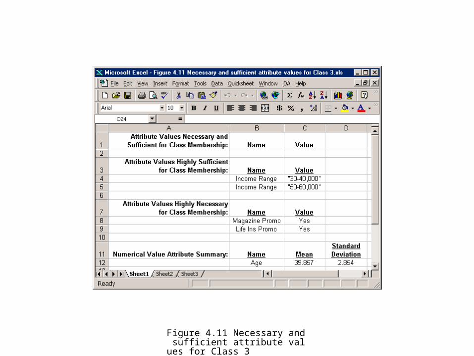
Figure 4.11 Necessary and sufficient attribute values for Class 3
Step 5: Visualize Individual Class Rules
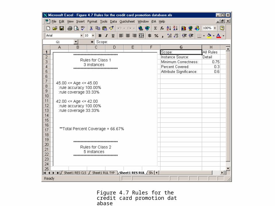
Figure 4.7 Rules for the credit card promotion database