Clustering short status messages: A topic model based

approach

by

Anand Karandikar

Thesis submitted to the Faculty of the Graduate Schoolof the University of Maryland in partial fulfillment

of the requirements for the degree ofMaster of Science

2010

ABSTRACT

Title of Thesis: Clustering short status messages: A topic model based approach

Anand Karandikar, Master of Science, 2010

Thesis directed by: Dr. Tim Finin, ProfessorDepartment of Computer Science andElectrical Engineering

Recently, there has been an exponential rise in the use of online social media systems

like Twitter and Facebook. Even more usage has been observedduring events related to

natural disasters, political turmoil or other such crises.Tweets or status messages are short

and may not carry enough contextual clues. Hence, applying traditional natural language

processing algorithms on such data is challenging. Topic model is a popular method for

modeling term frequency occurrences for documents in a given corpus. A topic basically

consists of set of words that co-occur frequently. Unsupervised nature allows topic models

to be trained easily on datasets meant for specific domains.

We use the topic modeling feature of MALLET - a machine learning tool kit, to gen-

erate topic models from unlabelled data. We propose a way to cluster tweets by using the

topic distributions in each tweet. We address the problem ofdetermining which topic model

is optimal for clustering tweets based on its clustering performances. We also demonstrate

a use case wherein we cluster Twitter users based on the content they tweet. We back our

research with experimental results and evaluations.

Keywords: topic models, clustering, social media, Twitter.

c© Copyright Anand Karandikar 2010

Dedicated to Aai, Baba and Amit.

ii

ACKNOWLEDGMENTS

I would like to express my sincere gratitude to my graduate advisor Dr. Tim Finin. I

thank him for his constant support and continuted belief in me. His suggestions, motivation

and advice were vital in bringing this work to completion.

I would like to thank Dr. Anupam Joshi and Dr. Charles Nicholasfor graciously

agreeing to be on my thesis committee.

A special note of thanks to Dr. Akshay Java, Justin Martineauand William Murnane

for suggestions, long discussions and providing timely help. I thank Dr. Kirill Kireyev

from University of Colorado at Boulder for his help regarding the R analysis package. I

would also like to thank my friends at eBiquity lab for their constant encouragement.

iii

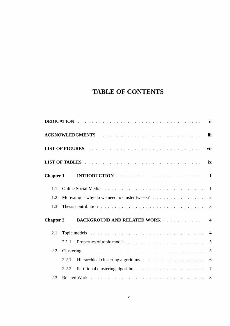
TABLE OF CONTENTS

DEDICATION . . . . . . . . . . . . . . . . . . . . . . . . . . . . . . . . . . . ii

ACKNOWLEDGMENTS . . . . . . . . . . . . . . . . . . . . . . . . . . . . . iii

LIST OF FIGURES . . . . . . . . . . . . . . . . . . . . . . . . . . . . . . . . vii

LIST OF TABLES . . . . . . . . . . . . . . . . . . . . . . . . . . . . . . . . . ix

Chapter 1 INTRODUCTION . . . . . . . . . . . . . . . . . . . . . . . . 1

1.1 Online Social Media . . . . . . . . . . . . . . . . . . . . . . . . . . . . . 1

1.2 Motivation - why do we need to cluster tweets? . . . . . . . . . .. . . . . 2

1.3 Thesis contribution . . . . . . . . . . . . . . . . . . . . . . . . . . . . . .3

Chapter 2 BACKGROUND AND RELATED WORK . . . . . . . . . . . 4

2.1 Topic models . . . . . . . . . . . . . . . . . . . . . . . . . . . . . . . . . 4

2.1.1 Properties of topic model . . . . . . . . . . . . . . . . . . . . . . . 5

2.2 Clustering . . . . . . . . . . . . . . . . . . . . . . . . . . . . . . . . . . . 5

2.2.1 Hierarchical clustering algorithms . . . . . . . . . . . . . .. . . . 6

2.2.2 Partitional clustering algorithms . . . . . . . . . . . . . . .. . . . 7

2.3 Related Work . . . . . . . . . . . . . . . . . . . . . . . . . . . . . . . . . 8

iv

2.3.1 Topic models for information discovery . . . . . . . . . . . .. . . 8

2.3.2 Text categorization . . . . . . . . . . . . . . . . . . . . . . . . . . 9

2.3.3 Topic models and online social media . . . . . . . . . . . . . . .. 10

Chapter 3 SYSTEM DESIGN AND IMPLEMENTATION . . . . . . . . 11

3.1 System Design . . . . . . . . . . . . . . . . . . . . . . . . . . . . . . . . 11

3.1.1 Topic modeler . . . . . . . . . . . . . . . . . . . . . . . . . . . . 11

3.1.2 Topic models generated from various configurations . .. . . . . . 13

3.1.3 Topic Vectors . . . . . . . . . . . . . . . . . . . . . . . . . . . . . 14

3.1.4 Clustering . . . . . . . . . . . . . . . . . . . . . . . . . . . . . . . 14

3.2 Datasets . . . . . . . . . . . . . . . . . . . . . . . . . . . . . . . . . . . . 15

3.2.1 Twitter dataset (twitterdb) . . . . . . . . . . . . . . . . . . . . .. 15

3.2.2 TAC KBP news wire corpus . . . . . . . . . . . . . . . . . . . . . 16

3.2.3 Disaster events dataset . . . . . . . . . . . . . . . . . . . . . . . . 17

3.2.4 Supplementary test dataset . . . . . . . . . . . . . . . . . . . . . .18

3.3 Tools and libraries . . . . . . . . . . . . . . . . . . . . . . . . . . . . . . .18

3.3.1 MALLET . . . . . . . . . . . . . . . . . . . . . . . . . . . . . . . 18

3.3.2 Twitter4j . . . . . . . . . . . . . . . . . . . . . . . . . . . . . . . 19

3.3.3 R analysis package . . . . . . . . . . . . . . . . . . . . . . . . . . 19

Chapter 4 EXPERIMENTAL ANALYSIS AND RESULTS . . . . . . . . 20

4.1 Definitions, computation techniques and analysis . . . . .. . . . . . . . . 20

4.1.1 Residual Sum of Squares (RSS) . . . . . . . . . . . . . . . . . . . 20

4.1.2 Cluster Cardinality . . . . . . . . . . . . . . . . . . . . . . . . . . 21

4.1.3 Cluster centers and iterations . . . . . . . . . . . . . . . . . . . .. 22

4.1.4 Cluster validation criterion . . . . . . . . . . . . . . . . . . . . .. 23

v

4.1.5 Clustering Accuracy . . . . . . . . . . . . . . . . . . . . . . . . . 24

4.2 Effect of change in topic model parameters on Jaccard coefficient . . . . . . 25

4.2.1 Effect of change in training data size . . . . . . . . . . . . . .. . . 25

4.2.2 Effect of change in training data corpus . . . . . . . . . . . .. . . 27

4.2.3 Effect of change in number of topics . . . . . . . . . . . . . . . .. 29

4.3 Selecting an optimal topic model . . . . . . . . . . . . . . . . . . . .. . . 30

4.4 Jaccard coefficient matrix . . . . . . . . . . . . . . . . . . . . . . . . .. . 33

4.5 Accuracy on test dataset . . . . . . . . . . . . . . . . . . . . . . . . . . .34

4.6 Applying topic model to cluster Twitter users . . . . . . . . .. . . . . . . 34

4.7 Limitations . . . . . . . . . . . . . . . . . . . . . . . . . . . . . . . . . . 35

Chapter 5 CONCLUSION AND FUTURE WORK . . . . . . . . . . . . 38

5.1 Conclusion . . . . . . . . . . . . . . . . . . . . . . . . . . . . . . . . . . 38

5.2 Future Work . . . . . . . . . . . . . . . . . . . . . . . . . . . . . . . . . . 39

REFERENCES . . . . . . . . . . . . . . . . . . . . . . . . . . . . . . . . . . . 40

vi

LIST OF FIGURES

2.1 Raw data for hierarchical clustering (figure courtsey: Wikipedia) . . . . . . 6

2.2 Dendrogram representation for hierarchical clustering (figure courtsey:

Wikipedia) . . . . . . . . . . . . . . . . . . . . . . . . . . . . . . . . . . 7

2.3 Demonstration of k-means clustering (figure courtsey: Wikipedia) . . . . . 8

3.1 System architecture . . . . . . . . . . . . . . . . . . . . . . . . . . . . . .12

3.2 Word to topic association for our training data set . . . . .. . . . . . . . . 13

3.3 Topic vectors snapshot for # topics = 200 . . . . . . . . . . . . . .. . . . 14

3.4 Clustering stage . . . . . . . . . . . . . . . . . . . . . . . . . . . . . . . . 15

3.5 Distribuition of tweet collection in twitterdb . . . . . . .. . . . . . . . . . 16

4.1 RSSmin v/s k . . . . . . . . . . . . . . . . . . . . . . . . . . . . . . . . . 23

4.2 Clustering with k = 8 on disaster events dataset using topic model trained

on TAC KBP news wire corpus with # topics=200 . . . . . . . . . . . . . . 24

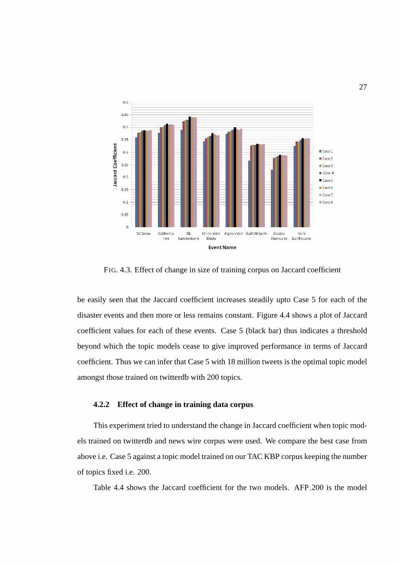
4.3 Effect of change in size of training corpus on Jaccard coefficient . . . . . . 27

4.4 Scatter plot of Jaccard coefficient for the disaster events dataset . . . . . . . 28

4.5 Effect of change in training data corpus on Jaccard coefficients for Case 5

and news wire trained topic model . . . . . . . . . . . . . . . . . . . . . . 29

4.6 Jaccard coefficient for topic models with varying topic number . . . . . . . 30

vii

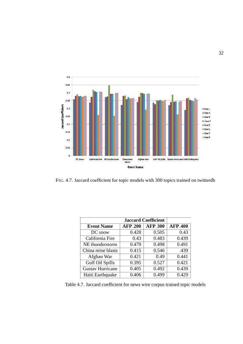
4.7 Jaccard coefficient for topic models with 300 topics trained on twitterdb . . 32

4.8 Comparing news wire trained topic models for 200, 300 and 400 topics . . 33

viii

LIST OF TABLES

3.1 Stop words list . . . . . . . . . . . . . . . . . . . . . . . . . . . . . . . . 12

3.2 Languages with more than 2% detection rate . . . . . . . . . . . .. . . . . 16

3.3 Top 10 hashtags and usertags . . . . . . . . . . . . . . . . . . . . . . . .. 17

3.4 Disaster events dataset . . . . . . . . . . . . . . . . . . . . . . . . . . .. 18

3.5 Supplementary test dataset . . . . . . . . . . . . . . . . . . . . . . . .. . 18

4.1 RSSmin and k for twitterdb trained topic model with 200 topics . . . . .. 22

4.2 Topic models with 200 topics trained using varying number of tweets from

twitterdb . . . . . . . . . . . . . . . . . . . . . . . . . . . . . . . . . . . . 26

4.3 Jaccard coefficient for various topic models with 200 topics trained using

twitterdb . . . . . . . . . . . . . . . . . . . . . . . . . . . . . . . . . . . . 26

4.4 Jaccard coefficient for Case 5 and topic model trained on TAC KBP news

wire corpus . . . . . . . . . . . . . . . . . . . . . . . . . . . . . . . . . . 28

4.5 Effect of change in number of topics . . . . . . . . . . . . . . . . . .. . . 30

4.6 Topic models with 300 topics trained using varying number of tweets from

twitterdb . . . . . . . . . . . . . . . . . . . . . . . . . . . . . . . . . . . . 31

4.7 Jaccard coefficient for news wire corpus trained topic models . . . . . . . . 32

4.8 Jaccard coefficient matrix for AFP300 . . . . . . . . . . . . . . . . . . . . 33

ix

4.9 Relation between most frequent words and topic keys . . . . .. . . . . . . 34

4.10 Clustering accuracy for test dataset . . . . . . . . . . . . . . . .. . . . . . 34

4.11 Twitter users . . . . . . . . . . . . . . . . . . . . . . . . . . . . . . . . . . 35

4.12 Twitter user clusters . . . . . . . . . . . . . . . . . . . . . . . . . . . .. . 36

4.13 Jaccard coefficient calculations for Case C . . . . . . . . . . .. . . . . . . 36

4.14 Topic model configurations with cluster cardinality6= 8 . . . . . . . . . . . 37

4.15 Jaccard coefficient calculations for Case D . . . . . . . . . . .. . . . . . . 37

x

Chapter 1

INTRODUCTION

In this chapter we present an introduction to the online social media. We will discuss

the need for clustering the data that is available on such social media sites and present a

formal thesis definition.

1.1 Online Social Media

Recently online social media has emerged as a medium of communication and infor-

mation sharing. Status updates, blogging, video sharing and social networking are some of

the ways in which people try to achieve this.

Popular online social media sites like Facebook1, Orkut2 or Twitter3 allow users to

post short message to their homepage. These are often referred as micro-blogging4 sites

and the message is called astatus update. Status updates from Twitter are more commonly

called as tweets. Tweets are often related to some event, specific topic of interest like music,

dance or personal thoughts and opinions. A tweet can containtext, emoticon, link or their

combination.

1http://www.facebook.com/2http://www.orkut.com/3http://twitter.com/4http://en.wikipedia.org/wiki/Microblogging

1

2

Tweets have recently gained a lot of importance due to their ability to disseminate

information rapidly. Popular search engines like Google5 and Bing6 have started including

feeds from Twitter in their search results. Researchers are actively involved in analyz-

ing these micro-blogging systems. Some research areas include understanding usage and

communities (Javaet al. 2007), discovering user characteristics (Dongwooet al. 2010),

detecting spam (Yardiet al. 2010) and so on.

1.2 Motivation - why do we need to cluster tweets?

Analysis of micro blogging sites during crises situation has seen a rising interest as

discussed in (Starbirdet al. 2010) and (Vieweget al. 2010). Content oriented analysis

by applying traditional natural language techniques usingsyntactic and semantic model is

difficult due to reasons described in (Kireyev, Palen, & Anderson 2009). These can be

summarized as

• Tweets are very short in length with the message length beingabout 140 characters.

Such a short piece of text provides very few contextual cluesfor applying machine

learning techniques.

• Tweets are written in informal style and often consist of simple phrases, sentence

fragments andor ungrammatical text. They contain abbreviations, internet slang and

mispelled words.

• Tweets may contain implied references to locations as described in (Vieweget al.

2010). Hence, named entity recognition using off the shelf named entity recognizers

yield poor results.

5http://www.google.com/6http://www.bing.com/

3

We believe that clustering of tweets will help to easily categorize them based on their

content. Using such clusters we would be able to identify thetopic or particular event about

which the tweet is.

In this work, we would thus like to define a process that will classify an incoming

tweet to one of the clusters existing in the system using topic model approach. Currently,

we have analyzed the clusters generated using differently trained topic models. These topic

models vary in size of training data, training data itself and number of topics.

1.3 Thesis contribution

The thesis contribution can be briefly stated as follows:

1. We determine the topic model configuration that is optimalto cluster tweets. Typ-

ically, in machine learning a model is trained using data that belongs to the same

domain as the test data. For example, a named entity recognition system for biology

related data is trained on biological data. But as mentioned above the short nature

and esoteric form of tweets makes it necessary to explore if atopic model trained on

twitter can yield better performance compared to a topic model trained on new wire

text which has more contextual information.

2. We then evaluate the decisions made in point 1 by clustering a new set of tweets and

also estimate the accuracy of the results. We compare the accuracy obtained with a

baseline approach to show the merit of topic model based approach.

3. We show that the use of topic model to cluster Twitter usersbased on their status

updates. We show the merit of topic model based approach to cluster Twitter users.

Chapter 2

BACKGROUND AND RELATED WORK

Generative models1 have been popular for document analysis. A generative modelis a

model for randomly generating observable data, typically given some hidden parameters. It

specifies a joint probability distribution over observation and label sequences. Often these

generative models talk about a special type called topic model. There has been some work

around analysis of Twitter data using topic models. In this chapter, we will explain few

background concepts that are necessary to understand this thesis work. We will also review

some recent research about analyzing online social media using topic models.

2.1 Topic models

Topic models are generative models and a popular method for modeling term fre-

quency occurrences for documents in a given corpus. The basic idea is to describe a doc-

ument as mixture of different topics. A topic is simply a collection of words that occur

frequently with each other.

Latent Dirichlet allocation (Blei, Ng, & Jordan 2003) is a generative model that allows

sets of observations to be explained by unobserved groups which explain why some parts

of the data are similar. For example, if observations are words collected into documents,

1http://en.wikipedia.org/wiki/Generativemodel

4

5

it posits that each document is a mixture of a small number of topics and that each word’s

creation is attributable to one of the document’s topics.

Latent semantic analysis (Landauer, Foltz, & Laham 1998) isa technique in natural

language processing, in particular in vectorial semantics, of analyzing relationships be-

tween a set of documents and the terms they contain by producing a set of concepts related

to the documents and terms.

2.1.1 Properties of topic model

As discussed in (Kireyev, Palen, & Anderson 2009), topic models have certain prop-

erties that make it suitable to analyze Twitter data. These are summarized below:

Topic models do not make any assumptions about the ordering of words (Steyver &

Griffiths 2007). This is known as bag-of-words model2. It disregards grammar as well. This

is particularly suitable to handle language and grammar irregularities in Twitter messages.

Each document is represented as a numerical vector that describes its distribution over

the topics. This representation is convenient to compute document similarity and perform

clustering.

Training a topic model is easy since it uses unsupervised learning. It saves the effort

required on creating labeled data and training classifiers using such labeled data.

Topic models are useful for identifying unobserved relationships in the data. This

makes dealing with abbreviations and misspellings easy by using topic models.

2.2 Clustering

Clustering is an unsupervised learning techniques that takes a collection of objects

such as tweets and organizes them into groups based on their similarity. The groups that are

2http://en.wikipedia.org/wiki/Bagof wordsmodel

6

FIG. 2.1. Raw data for hierarchical clustering (figure courtsey:Wikipedia)

formed are known as clusters. Let’s take a look at two main types of clustering algorithms.

2.2.1 Hierarchical clustering algorithms

This type of clustering algorithms can be divided into two types.

Agglomerative (bottom-up): Agglomerative algorithms begin with each individual docu-

ment as a separate cluster, each of size one. At each level thesmaller clusters are merged

to form a larger cluster. It proceeds this way until all the clusters are merged into a single

cluster that contains all the documents.

Divisive (top-down): Divisive algorithms begin with the entire set and then the splits are

performed to generate successive smaller clusters. It proceeds recursively until individual

documents are reached.

The agglomerative algorithms are more frequently used in information retrieval than

the divisive algorithms. The splits and merge are generallydone using a greedy algorithm.

A greedy algorithm is an algorithmic approach that makes thelocally optimal choice at

each stage of its run with the hope of finding the global optimum. The results are often

represented using a dendrogram as shown in Figure 2.2.

7

FIG. 2.2. Dendrogram representation for hierarchical clustering (figure courtsey:Wikipedia)

2.2.2 Partitional clustering algorithms

Partitional clustering algorithms typically determine all clusters at once. The k-means

clustering algorithm belongs to this category. It starts off with choosing ’k’ clusters and

then assigning each data point to the cluster whose center isnearest. The algorithm as

described in (MacQueen 1967) is as follows:

1. Choose the number of clusters, k.

2. Randomly generate k clusters and determine the cluster

centers, or directly generate k random points as

cluster centers.

3. Assign each point to the nearest cluster center, where

"nearest" is defined with respect to one of the

distance measures discussed above.

4. Recompute the new cluster centers.

5. Repeat the two previous steps until some convergence

criterion is met (usually that the assignment

hasn’t changed).

8

FIG. 2.3. Demonstration of k-means clustering (figure courtsey: Wikipedia)

The main advantages of k-means are its simplicity and speed when applied to large

data sets. The most common hierarchical clustering algorithms have a complexity that is

at least quadratic in the number of documents compared to thelinear complexity of k-

means. K-means is linear in all relevant factors: iterations, number of clusters, number of

vectors and dimensionality of the space. This means that k-means is more efficient than the

hierarchical algorithms as described in (Manning, Raghavan, & Schutze 2008). Figure 2.3

gives a demonstration for a k-means algorithm.

2.3 Related Work

Topic models have been applied to a number of tasks that are relevant to our goal of

clustering Twitter status messages. We will briefly describe three categories and cite a few

examples in each.

2.3.1 Topic models for information discovery

There has been some work with regards to using topic models for information discov-

ery. (Phan, Nguyen, & Horiguchi 2008) presents a framework to build classifiers using both

a set of labelled training data and hidden topics discoveredfrom large scale data collections.

9

It provides a general framework to be applied across different data domains. (Griffiths &

Steyvers 2004) presents a generative model to discover topics covered by papers in PNAS3.

These topics were then used to identify relationships between various science disciplines

and finding latest trends. An unsupervised algorithm described in (Steyvers, Griffiths, &

Smyth 2004) extracts both the topics expressed in large textcollection and models how

the authors of the documents use those topics. Such author-topic models can be used

to discover topic trends, finding authors who most likely tend to write on certain topics

and so on. Author-Recipient-Topic model (McCallum, Corrada-Emmanuel, & Wang ), is a

Bayesian model for social network analysis that discovers topics in discussions conditioned

on sender-recipient relationships in the corpus.

2.3.2 Text categorization

Another set of research deals with similarity and categorization of texts. Use of

Wikipedia concepts to determine closeness between texts was explained in (Gabrilovich

& Markovitch 2007). Text categorization based on word clustering algorithms was de-

scribed in (Bekkermanet al. 2003). k-means clustering for sparse data was introduced

in (Dhillon & Modha 2001). A topic vector based space model for document comparison

was introduced in (Kuropka & Becker 2003). (Lee, Wang, & Yu ) explores supervised and

unsupervised approaches to detect topic in biomedical textcategorization. It describes the

Naive Bayes based approach to assign text to predefined topics. It performs topic based

clustering using unsupervised hierarchical clustering algorithms.

3Proceedings of the National Academy of Sciences of the United States of America, http://www.pnas.org/

10

2.3.3 Topic models and online social media

As described in Chapter 1, most of the work related to Twitter and online social media

in general has been focused on understanding usage and communities (Javaet al. 2007), the

role of micro-blogging (Zhao & Rosson 2009) and other such aspects related to community

and network structure. Recent research has started to look atcontent related aspects of

online social media and specifically Twitter. Smarter BlogRoll (Baumer & Fisher ), uses

text mining techniques to augment a blogroll with information about current topics of the

blogs in that blog roll. The use of a partially supervised learning model (Labeled LDA)

to characterize Twitter data and users is presented in (Ramage, Dumais, & Liebling ). It

classifies tweets based on roughly four dimensions like substance, style, social and status.

Topic based clustering approach mentioned in (Kireyev, Palen, & Anderson 2009) identifies

latent patterns like informational and emotional messagesin earthquake and tsunami data

sets collected from Twitter.

Chapter 3

SYSTEM DESIGN AND IMPLEMENTATION

In this chapter we will explain a high level design and implementation of our system.

In the first section we explain the system components that have most direct influence on

the system. We then describe the datasets, libraries and packages that we used to build this

system.

3.1 System Design

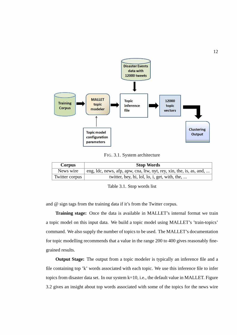
Figure 3.1 provides an architectural overview of our system.

3.1.1 Topic modeler

This is the most important block in our system. A topic modeler consists of three

stages.

Input stage: This stage involves converting the training corpus into an acceptable

format. MALLET (McCallum 2002) that we used to build our system provides a special

input command for converting the training data into MALLET’s special internal format. We

also remove certain stop words from the corpus during this stage. Since we have build topic

models from new wire corpus and Twitter corpus which we describe in the next section;

we have used two different lists of stop words as shown in Table 3.1. We also remove url’s

11

12

FIG. 3.1. System architecture

Corpus Stop WordsNews wire eng, ldc, news, afp, apw, cna, ltw, nyt, rey, xin, the, is, as,and, ...

Twitter corpus twitter, hey, hi, lol, lo, i, get, with, the, ...

Table 3.1. Stop words list

and @ sign tags from the training data if it’s from the Twittercorpus.

Training stage: Once the data is available in MALLET’s internal format we train

a topic model on this input data. We build a topic model using MALLET’s ’train-topics’

command. We also supply the number of topics to be used. The MALLET’s documentation

for topic modelling recommends that a value in the range 200 to 400 gives reasonably fine-

grained results.

Output Stage: The output from a topic modeler is typically an inference fileand a

file containing top ’k’ words associated with each topic. We use this inference file to infer

topics from disaster data set. In our system k=10, i.e., the default value in MALLET. Figure

3.2 gives an insight about top words associated with some of the topics for the news wire

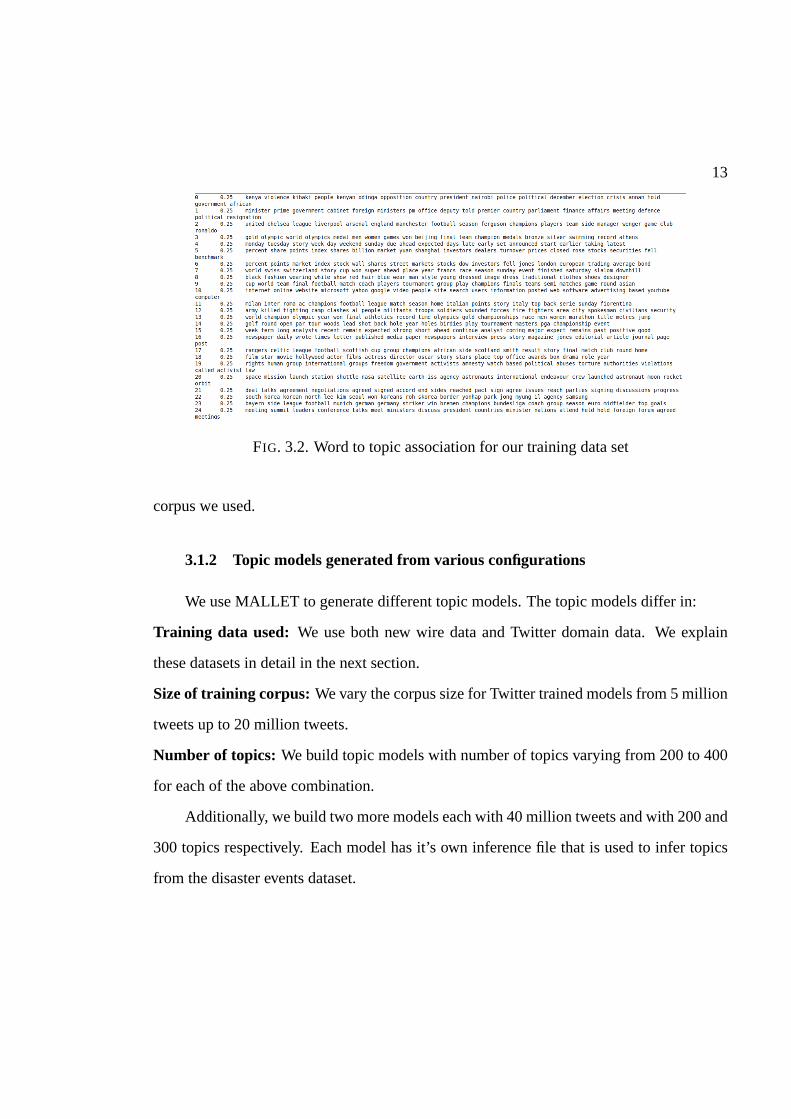
13

FIG. 3.2. Word to topic association for our training data set

corpus we used.

3.1.2 Topic models generated from various configurations

We use MALLET to generate different topic models. The topic models differ in:

Training data used: We use both new wire data and Twitter domain data. We explain

these datasets in detail in the next section.

Size of training corpus: We vary the corpus size for Twitter trained models from 5 million

tweets up to 20 million tweets.

Number of topics: We build topic models with number of topics varying from 200 to 400

for each of the above combination.

Additionally, we build two more models each with 40 million tweets and with 200 and

300 topics respectively. Each model has it’s own inference file that is used to infer topics

from the disaster events dataset.

14

FIG. 3.3. Topic vectors snapshot for # topics = 200

3.1.3 Topic Vectors

MALLET provides an option to use a previously generated inference file as an infer-

ence tool. The output is a topic vector which gives a distribution over each topic for every

document. Figure 3.3 gives a snapshot of topic vectors generated for one such document

from a topic model trained on news wire corpus and 200 topics.

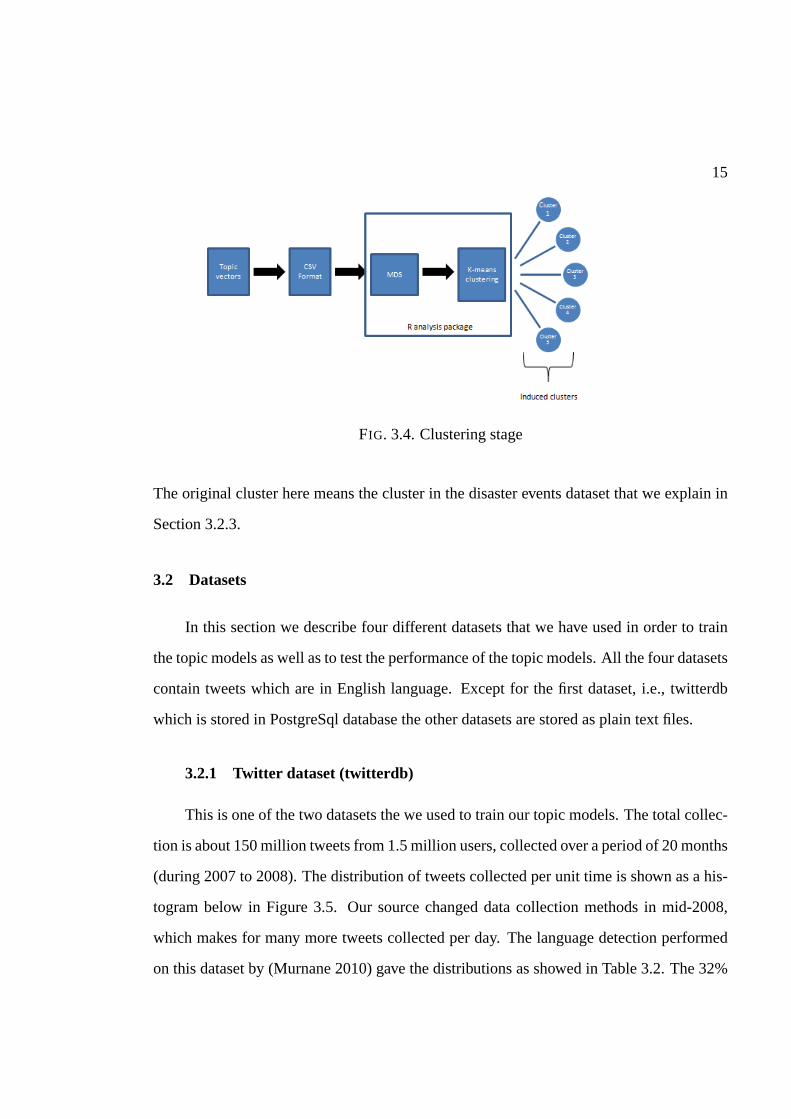
3.1.4 Clustering

We use R (R Development Core Team 2010), a system for statistical analysis and

graphics for clustering the tweets based on their topic vectors. We first convert the file

containing topic vectors to comma-separated values (CSV) format so that it is suitable for

processing with R’s commands. We then perform multidimensional scaling (MDS) (Cox

& Cox 2001) on this data to reduce it to two dimensions using R’scmdscalefunction.

MDS is a common way to visualize an N-dimensional data for exploring similarities and

dissimilarities in it. We then perform clustering on these reduced dimensions using R’s

k-meansfunction. Figure 3.4 provides a closer look at the clustering stage.

The k-meanscommand in R returns a vector containing cluster association for each

document in the dataset. We run a program to collect togetherall the documents with same

cluster numbers. For such an induced cluster, if more than 50% of the documents belong

to a particular original cluster then we assign the induced cluster with that event name.

15

FIG. 3.4. Clustering stage

The original cluster here means the cluster in the disaster events dataset that we explain in

Section 3.2.3.

3.2 Datasets

In this section we describe four different datasets that we have used in order to train

the topic models as well as to test the performance of the topic models. All the four datasets

contain tweets which are in English language. Except for thefirst dataset, i.e., twitterdb

which is stored in PostgreSql database the other datasets are stored as plain text files.

3.2.1 Twitter dataset (twitterdb)

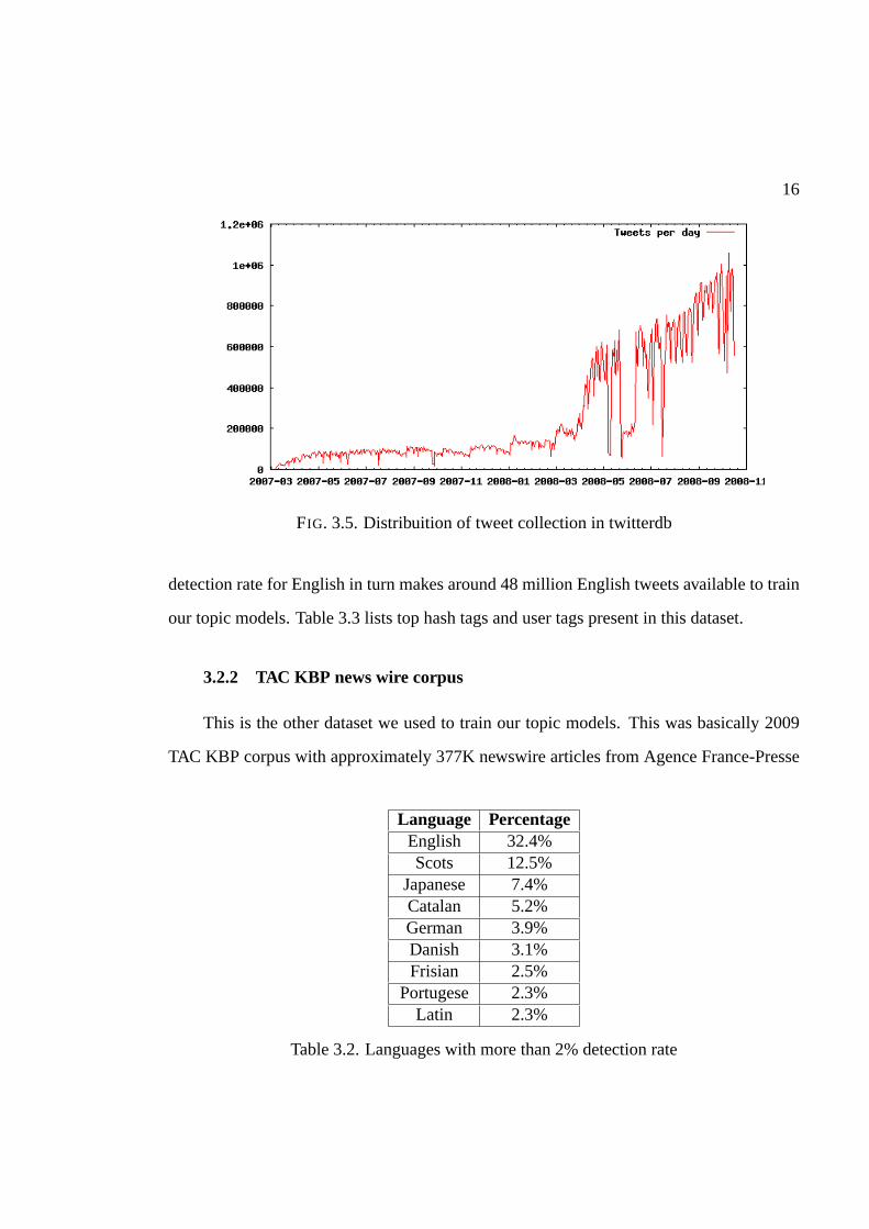
This is one of the two datasets the we used to train our topic models. The total collec-

tion is about 150 million tweets from 1.5 million users, collected over a period of 20 months

(during 2007 to 2008). The distribution of tweets collectedper unit time is shown as a his-

togram below in Figure 3.5. Our source changed data collection methods in mid-2008,

which makes for many more tweets collected per day. The language detection performed

on this dataset by (Murnane 2010) gave the distributions as showed in Table 3.2. The 32%

16

FIG. 3.5. Distribuition of tweet collection in twitterdb

detection rate for English in turn makes around 48 million English tweets available to train

our topic models. Table 3.3 lists top hash tags and user tags present in this dataset.

3.2.2 TAC KBP news wire corpus

This is the other dataset we used to train our topic models. This was basically 2009

TAC KBP corpus with approximately 377K newswire articles from Agence France-Presse

Language PercentageEnglish 32.4%Scots 12.5%

Japanese 7.4%Catalan 5.2%German 3.9%Danish 3.1%Frisian 2.5%

Portugese 2.3%Latin 2.3%

Table 3.2. Languages with more than 2% detection rate

17

Hashtags 1, 2, 1:, news, 3news, rnc08, elecoes, 080808,dnc08, lastfm

Usertags chrisbrogan, garyvee, commuter, harunyan,leolaporte, lynmock, kazusap, kevinrose, Scobleizer, Hemi

Table 3.3. Top 10 hashtags and usertags

(AFP). About half articles were from 2007 and half from 2008 with a few (less than 1%)

from 1994-2006.

3.2.3 Disaster events dataset

This dataset includes tweets for 8 disaster events as shown in Table 3.4. We collected

1500 tweets for each of these events which gave us a total of 12,000 tweets in this dataset.

The tweets for two events, namely,California FiresandGustav Hurricanewere from our

Twitter dataset. We exclude these tweets while training themodel using Twitter dataset.

The tweets for the other six events were obtained from Twitter’s public timeline using

twitter4j 2. We have used a number of Twitter search operators to get the most accurate

query for the events. Here are some of the examples queries.

• Using words, hashtags and date ranges for querying

Haiti earthquake in Jan 2010: haiti earthquake # haiti since:2010-01-12 until:2010-

01-16

• Using words, date ranges and location

Washington DC snow blizzard in Feb 2010: snow since:2010-02-25 until:2010-02-

28 near:”Washington DC” within:25mi

A manual scan for tweets from five events, namelyAfghanistan war, China mine

blasts, California fires, Haiti earthquakeandDC snowindicates that more than 97% tweets

2http://twitter4j.org/en/index.html

18

Event name SourceDC snow Twitter search API’s

NE thuderstorm Twitter search API’sHaiti earthquake Twitter search API’sAfghanistan war Twitter search API’sChina mine blasts Twitter search API’s

Gulf oil spill Twitter search API’sCalifornia fires twitterdb

Gustav hurricane twitterdb

Table 3.4. Disaster events dataset

Event #TweetsHurricance Alex 624China earthquake 376

Table 3.5. Supplementary test dataset

are actually related to those particular events. Thus we caninfer that this data contains eight

clusters. We call this as ’original clusters’ in further chapters.

3.2.4 Supplementary test dataset

We collected 1000 tweets which were a mixture of tweets from Hurricane Alex of

June 2010 and China earthquake of May 2008. We manually went through all these 1000

tweets and confirmed their relevance to either of the events.Table 3.5 shows the tweet

distribution.

3.3 Tools and libraries

3.3.1 MALLET

MALLET stands for MAchine Learning for LanguagE Toolkit andis a opensource

software toolkit. It provides a Java-based package to do various machine learning tasks.

We use the topic modeling features as described in previous section. It provides a fast and

19

scalable implementation of Gibbs sampling and topic inferring tools.

3.3.2 Twitter4j

It provides a opensource Java library for Twitter API’s. We used it to collect tweets

related to disaster events. We have primarily used Search, Query and QueryResult imple-

mentation from the twitter4j package.

3.3.3 R analysis package

The R analysis package is a free software environment for statistical computing and

graphics. We typically use R’sdist command to perform distance matrix computations,

cmdscalecommand for multidimensional scaling andk-meanscommand for clustering. R

provides other commands that help to obtain within cluster sum of squares for each cluster,

cluster centroids, cluster size and a vector containing integers to indicate cluster association

for each data point.

Chapter 4

EXPERIMENTAL ANALYSIS AND RESULTS

In this chapter we present the results of the experiments performed for selecting the

best topic model for clustering Twitter data. We also present the clustering results for this

best topic model. We also provide results of our experimentsto cluster Twitter users using

this topic model.

Most of the code was in Java with some file handling and regularexpression matching

done using Perl scripts or shell commands. Clustering scripts were written in R language.

Clustering experiments were performed on Sun Solaris machine running Ubuntu OS with

about 40 GB RAM. Topic models were created on Linux machine with about 4 GB RAM.

4.1 Definitions, computation techniques and analysis

4.1.1 Residual Sum of Squares (RSS)

As defined in (Manning, Raghavan, & Schutze 2008), RSS is the squared distance

of each vector from it’s cluster centroid summed over all vectors in the cluster. It gives a

measure of how well the centroid represents a cluster. It’s aheuristic method to calculate

number of clusters for k-means clustering algorithm. It’s the objective funciton for k-means

and a smaller value of RSS indicates tighter clusters. RSS for thekth cluster is given by

equation 4.1.

20

21

RSSk =∑

~x∈ωk

|~x− ~µ(ωk)|2 (4.1)

where~x represents a distance vector of a document in clusterω and~µ(ωk) represents

the centroid of clusterωk given by equation 4.2.

~µ(ωk) =1

|ω|

∑

~x∈ω

~x (4.2)

Hence, the RSS for a particular clustering output with say K clusters is given by

RSS =K∑

k=1

RSSk (4.3)

4.1.2 Cluster Cardinality

As mentioned above we use a heuristic based approach to calculate value of k for k-

means clustering. We use the steps mentioned in (Manning, Raghavan, & Schutze 2008) to

find k.

• Perform i (we use i = 10) clusterings with a said value of k. Find the RSS in each

case as defined by equation 4.3.

• Find the minimum RSS value. Denote it asRSSmin.

• FindRSSmin for different values of k as k increases.

• Find the ’knee’ in the curve i.e. the point where successive decrease in this value is

the smallest. This value of k indicates the cluster cardinality.

Table 4.1 showsRSSmin for different values of k obtained for clustering using twit-

terdb trained topic model with 200 topics. Figure 4.1 shows the corresponding plot of

22

RSSmin k0.6903 30.4220 40.3662 50.2581 60.2391 70.2192 80.2098 90.1594 100.1469 110.1204 120.0999 13

Table 4.1.RSSmin and k for twitterdb trained topic model with 200 topics

RSSmin v/s k. It can be clearly observed from table 4.1 as well as Figure 4.1 that atk = 8

the curve flattens the most. Hence,k = 8 is the optimal cluster cardinality.

4.1.3 Cluster centers and iterations

As mentioned in Chapter 3, we use k-means command from R analysis package for

clustering. We use the following command syntax:

kmeans(dist, centers)

where,

dist : data matrix,

centers : number of cluster centers i.e.k

Cluster centers are randomly chosen from the set of rows available in dist. The number

of iterations performed to reach convergence is by default set to ten. We generated over 27

topic model configurations and have performed clustering. We found that barring just three

cases convergence was achieved with this setting. For thesethree cases we had to set this

value to 15 to allow k-means to reach convergence. The (Hartigan & Wong 1979) k-means

23

FIG. 4.1.RSSmin v/s k

clustering algorithm is used by default. Figure 4.2 shows the k-means clustering for our

disaster event dataset withk = 8 using topic model trained on TAC KBP news wire corpus

with 200 topics.

4.1.4 Cluster validation criterion

We validate the quality of induced clusters on:

• Cluster cardinality computed as in Section 4.1.2

• Similarity between clusters induced using k-means and original clusters (tweets from

eight different events) in the dataset using the Jaccard similarity coefficient

Jaccard similarity coefficient

Jaccard coefficient (Jaccard 1901) is a classic statisticalmeasure for similarity in sets. It is

defined as:

24

FIG. 4.2. Clustering with k = 8 on disaster events dataset using topic model trained onTAC KBP news wire corpus with # topics=200

J(A,B) = |A∩B||A∪B|

Practically, it can be easily computed by countingNAB = |A∩B| andNA andNB as

the data elements that belong only to set A and B respectivelyso thatNA +NB +NAB =

|A ∪ B| and hence

J(A,B) = NAB

NA+NB+NAB

In further sections, we use Jaccard coefficient as a measure for clustering performance

of a topic model. Higher the Jaccard coefficient value, more is an induced cluster similar

to an original cluster for the same kind of event.

4.1.5 Clustering Accuracy

As described in (Choudhary & Bhattacharyya ) we measure clustering accuracy using

the formula:

25

Accuracy = Numberofdocumentscorrectlyclusterd

Totalnumberofdocuments

We determine accuracy on the test dataset and the results arepublished in Section 4.5.

4.2 Effect of change in topic model parameters on Jaccard coefficient

We conducted three separate experiments to observe the effect of change of training

data size, training data type (twitterdb or news wire data) and changing the number of

topics to build a topic model on the Jaccard similarity coefficient. The Jaccard similarity

coefficient was calculated based on the comparison between induced clusters and original

clusters in the disaster events dataset as described in Section 3.2.3. In these experiments we

consider only those topic models that give us induced cluster count same as original cluster

count i.e 8. We address the case of inequality in induced cluster count and original cluster

count in Section 4.7.

4.2.1 Effect of change in training data size

We build nine different topic models using varying size of twitterdb data to train the

model. All the models have topic number fixed to 200. In one case, the topic model trained

on 15 million tweets from our twitterdb returned nine induced clusters on our disaster

events dataset. We ignore this particular case for this experiment.

Table 4.2 shows various topic models we trained using varying number of tweets from

our twitterdb collection. All the topic models shown have 200 topics. These topic models

were then used to perform clustering on the disaster events dataset which contained tweets

from eight events as described in Section 3.2.3. We calculate Jaccard similarity coefficient

in each case and the results are as shown in Table 4.3.

We then plot a bar graph as show in Figure 4.3 for the results inTable 4.3. It can

26

Topic model Number of tweets used (in millions)Case 1 5Case 2 10Case 3 16Case 4 17Case 5 18Case 6 19Case 7 20Case 8 40

Table 4.2. Topic models with 200 topics trained using varying number of tweets fromtwitterdb

Jaccard CoefficientEvent Name Case 1 Case 2 Case 3 Case 4 Case 5 Case 6 Case 7 Case 8DC snow 0.36 0.378 0.381 0.387 0.388 0.386 0.387 0.388California Fire 0.378 0.4 0.402 0.409 0.415 0.41 0.412 0.411NE thunderstorm 0.389 0.425 0.428 0.431 0.443 0.441 0.44 0.439China mine blasts 0.344 0.355 0.372 0.366 0.377 0.373 0.368 0.368Afghan War 0.374 0.382 0.385 0.391 0.401 0.393 0.391 0.394Gulf Oil Spills 0.267 0.327 0.33 0.329 0.334 0.333 0.331 0.333Gustav Hurricane 0.23 0.276 0.28 0.285 0.29 0.288 0.288 0.287Haiti Earthquake 0.326 0.354 0.343 0.35 0.357 0.354 0.355 0.356

Table 4.3. Jaccard coefficient for various topic models with200 topics trained usingtwitterdb

27

FIG. 4.3. Effect of change in size of training corpus on Jaccard coefficient

be easily seen that the Jaccard coefficient increases steadily upto Case 5 for each of the

disaster events and then more or less remains constant. Figure 4.4 shows a plot of Jaccard

coefficient values for each of these events. Case 5 (black bar)thus indicates a threshold

beyond which the topic models cease to give improved performance in terms of Jaccard

coefficient. Thus we can infer that Case 5 with 18 million tweets is the optimal topic model

amongst those trained on twitterdb with 200 topics.

4.2.2 Effect of change in training data corpus

This experiment tried to understand the change in Jaccard coefficient when topic mod-

els trained on twitterdb and news wire corpus were used. We compare the best case from

above i.e. Case 5 against a topic model trained on our TAC KBP corpus keeping the number

of topics fixed i.e. 200.

Table 4.4 shows the Jaccard coefficient for the two models. AFP 200 is the model

28

FIG. 4.4. Scatter plot of Jaccard coefficient for the disaster events dataset

Jaccard CoefficientEvent Name Case 5 AFP 200

DC snow 0.388 0.428California Fire 0.415 0.43

NE thunderstorm 0.44 0.479China mine blasts 0.377 0.415

Afghan War 0.401 0.421Gulf Oil Spills 0.334 0.395

Gustav Hurricane 0.29 0.405Haiti Earthquake 0.357 0.406

Table 4.4. Jaccard coefficient for Case 5 and topic model trained on TAC KBP news wirecorpus

29

FIG. 4.5. Effect of change in training data corpus on Jaccard coefficients for Case 5 andnews wire trained topic model

trained on TAC KBP corpus with 200 topics. Figure 4.5 shows a bar graph used to compare

the models. As we can see, news wire corpus gave good cluster similarity measure compare

to Case 5. We observed a similar behavior with topic models having 300 topics. Thus in

general we can infer that models trained on news wire corpus performed better compared to

models trained on Twitter data. Thus result gains added evidence from the fact that tweets

are short and esoteric and have very less contextual contentcompared to news wire text as

mentioned in Chapter 1.

4.2.3 Effect of change in number of topics

In this experiment we compared the Jaccard coefficients obtained by keeping the train-

ing corpus size and data constant and build topic models with200, 300 and 400 topics. Ta-

ble 4.5 shows the Jaccard coefficient values obtained for topic models trained using same

16 million tweets from our twitterdb but varying the topic numbers.

30

Jaccard CoefficientEvent Name T 200 T 300 T 400

DC snow 0.381 0.391 0.385California Fire 0.402 0.419 0.409

NE thunderstorm 0.428 0.447 0.435China mine blasts 0.372 0.382 0.38

Afghan War 0.385 0.4 0.396Gulf Oil Spills 0.33 0.353 0.349

Gustav Hurricane 0.298 0.388 0.324Haiti Earthquake 0.343 0.369 0.353

Table 4.5. Effect of change in number of topics

FIG. 4.6. Jaccard coefficient for topic models with varying topic number

It can be seen from the graph in Figure 4.6 that topic model (T300 indicated with

red bar) with 300 topics gives a peak performance. Experiments using news wire corpus

also yielded similar results. We found this result similar to those discussed in (Griffiths

& Steyvers 2004) and (Steyvers, Griffiths, & Smyth 2004), where a topic model with 300

topics was found to be optimal.

4.3 Selecting an optimal topic model

Section 4.2 demonstrates effect of changing various topic model parameters on the

Jaccard coefficient. Table 4.4 clearly shows that a topic model with 200 topics trained on

31

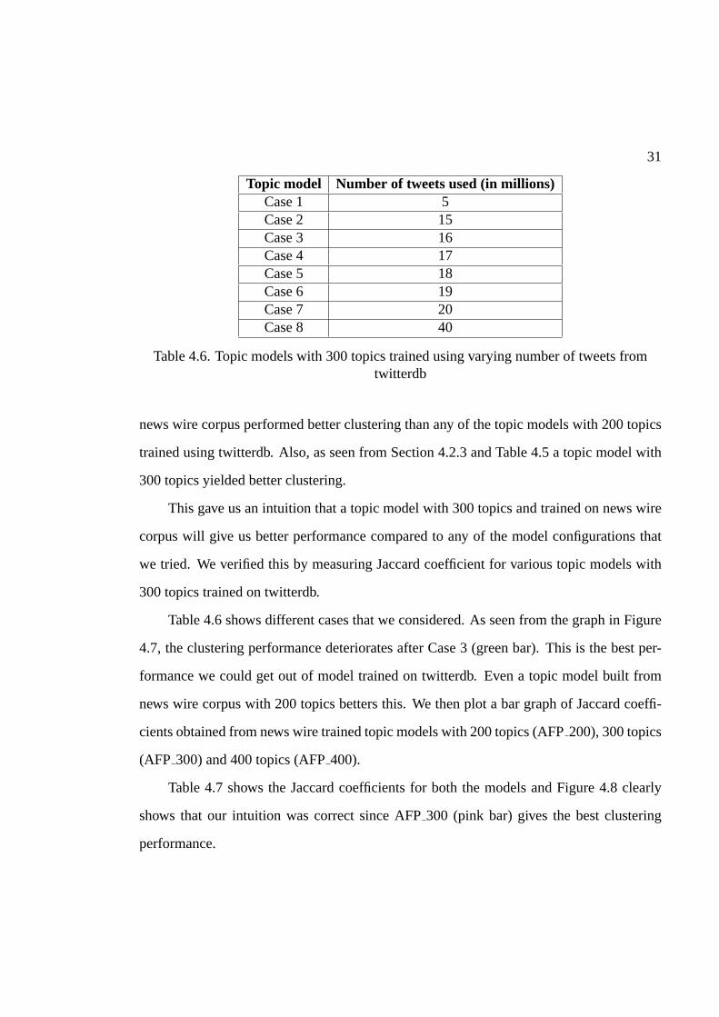
Topic model Number of tweets used (in millions)Case 1 5Case 2 15Case 3 16Case 4 17Case 5 18Case 6 19Case 7 20Case 8 40

Table 4.6. Topic models with 300 topics trained using varying number of tweets fromtwitterdb

news wire corpus performed better clustering than any of thetopic models with 200 topics

trained using twitterdb. Also, as seen from Section 4.2.3 and Table 4.5 a topic model with

300 topics yielded better clustering.

This gave us an intuition that a topic model with 300 topics and trained on news wire

corpus will give us better performance compared to any of themodel configurations that

we tried. We verified this by measuring Jaccard coefficient for various topic models with

300 topics trained on twitterdb.

Table 4.6 shows different cases that we considered. As seen from the graph in Figure

4.7, the clustering performance deteriorates after Case 3 (green bar). This is the best per-

formance we could get out of model trained on twitterdb. Evena topic model built from

news wire corpus with 200 topics betters this. We then plot a bar graph of Jaccard coeffi-

cients obtained from news wire trained topic models with 200topics (AFP200), 300 topics

(AFP 300) and 400 topics (AFP400).

Table 4.7 shows the Jaccard coefficients for both the models and Figure 4.8 clearly

shows that our intuition was correct since AFP300 (pink bar) gives the best clustering

performance.

32

FIG. 4.7. Jaccard coefficient for topic models with 300 topics trained on twitterdb

Jaccard CoefficientEvent Name AFP 200 AFP 300 AFP 400

DC snow 0.428 0.505 0.43California Fire 0.43 0.483 0.439

NE thunderstorm 0.479 0.498 0.491China mine blasts 0.415 0.546 .439

Afghan War 0.421 0.49 0.441Gulf Oil Spills 0.395 0.527 0.421

Gustav Hurricane 0.405 0.492 0.439Haiti Earthquake 0.406 0.499 0.429

Table 4.7. Jaccard coefficient for news wire corpus trained topic models

33

FIG. 4.8. Comparing news wire trained topic models for 200, 300 and 400 topics

Original ClustersDC snow California Fire NE Thunderstorm China mine blasts Afghan War Gulf Oil Spills Gustav Hurricane Haiti Earthquake

Induced ClustersDC snow 0.505 0.028 0.231 0.016 0.009 0.046 0.12 0.048

California Fire 0.024 0.483 0.042 0.127 0.139 0.08 0.046 0.061NE thunderstorm 0.141 0.012 0.498 0.004 0.016 0.111 0.213 0.009China mine blasts 0.008 0.092 0.016 0.546 0.21 0.024 0.003 0.101

Afghan War 0.019 0.124 0.026 0.136 0.49 0.016 0.097 0.098Gulf Oil Spills 0.089 0.071 0.009 0.066 0.117 0.527 0.018 0.083

Gustav Hurricane 0.178 0.061 0.18 0.037 0.002 0.096 0.492 0.101Haiti Earthquake 0.051 0.134 0.003 0.108 0.09 0.101 0.014 0.499

Table 4.8. Jaccard coefficient matrix for AFP300

4.4 Jaccard coefficient matrix

In the previous section we concluded that AFP300 has the best performance for the

task of clustering tweets. Table 4.8 provides us an insight about what proportion of each

events is an induced cluster made up of.

We observed that the induced cluster forNE thunderstormhas the second highest con-

tribution from tweets related toGustav Hurricane. Similar was the case with induced clus-

ters forAfghan Warhaving second highest contribution from tweets related toCalifornia

Fire and vice versa. To analyze this behavior we generated a list of top five most frequent

words for these events from our disaster events dataset by ignoring the proper nouns. For

example, we ignore proper nouns like California, CA, USA and Gustav. We then investi-

gated the topic keys generated by MALLET for AFP300 topic model. We found that in

34

Induced Cluster for Top 5 most frequent words from disaster events dataset topic keys generated by MALLETAfghan War war, fires, army, terrorist, kill fire, california, fires, damage, police

California Fire fire, burn, smoke, damage, west killed, shot, attack, died, injured, woundedNE thunderstorm storm, winds, rain, warning, people storm, people, hurricane, rain, rains, flooding, floodGustav Hurricane hurricane, storm, floods, heavy, weather coast mexico, areas

Table 4.9. Relation between most frequent words and topic keys

Cluster Name Size of induced cluster (A) Correctly clustered tweets (A∩ B) Original Size (B) Jaccard Coefficient AccuracyHurricane Alex 572 403 624 0.508 64.58%

China earthquake 428 263 376 0.486 69.94%

Table 4.10. Clustering accuracy for test dataset

some topics these words co-occurred. Table 4.9 shows the most frequent words and related

topic keys.

4.5 Accuracy on test dataset

We determined the accuracy of AFP300 by using it to cluster test dataset described in

Section 3.2.4. We obtained an accuracy of about64% for clustering tweets fromHurricane

Alexand about70% for clustering tweets fromChina earthquake.

The baseline we chose was the framework built to classify sparse and short text by

(Phan, Nguyen, & Horiguchi 2008). It uses a a training corpusof around 22.5K documents

for training and 200 topics with Gibbs sampling. They had an accuracy of around 67% to

classify short pieces text from medicinal domain.

We present these results in Table 4.10. It can also be observed that the Jaccard co-

efficient values forHurricane AlexandChina earthquakeare similar to those forGustav

HurricaneandHaiti Earthquakerespectively as shown in Table 4.7 for AFP300.

4.6 Applying topic model to cluster Twitter users

We use AFP300 to perform an experiment of clustering Twitter users based on their

tweets. We identified 21 well known Twitter users across seven different domains - sports,

35

Domain Twitter userSports @ESPN, @Lakers, @NBA

Travel Reviews @Frommers, @TravBuddy, @mytravelguideFinance @CBOE, @CNNMoney, @nysemoneysenseMovies @imdb, @peoplemag, @RottenTomatoes, @eonline

Technology News @TechCrunch, @diggtechnewsGaming @EASPORTS, @IGN, @NeedforSpeed

Breaking News @foxnews, @msnbc, @abcnews

Table 4.11. Twitter users

travel reviews, finance, movies, technology news, gaming and breaking news. We used

Twellow1 to obtain Twitter users. It’s like a yellow pages for Twitter. Table 4.11 shows the

Twitter users we selected for this experiment. We collected100 tweets for each user using

Twitter API.

We generate topic vector for a user by aggregating the topic dimensions across all the

tweets for that user. Table 4.12 shows the clustering results. k = 6 was experimentally

obtained as the optimal value ofk by performing cluster cardinality analysis as described

in Section 4.1.2.

@EASPORTS consisted more tweets about it’s new NBA and football game release. It

ended up being clusterd with other sports domain users. Technology news related users and

breaking news got clustered together with @msnbc ending up with other finance domain

users.

4.7 Limitations

We are aware of two limitations in our work. The first concernsour approach for

evaluating the accuracy of the induced clusters which, in some cases, could not be applied.

The second involves the lack of tests for the statistical significance of some of our results.

1http://www.twellow.com/

36

Cluster # Twitter users1 @CBOE, @msnbc, @CNNMoney, @nysemoneysense2 @IGN, @NeedforSpeed3 @EASPORTS, @ESPN, @Lakers, @NBA4 @Frommers, @TravBuddy, @mytravelguide5 @imdb, @peoplemag, @RottenTomatoes, @eonline6 @foxnews, @abcnews, @TechCrunch, @diggtechnews

Table 4.12. Twitter user clusters

Cluster Type K-means (A) Original (B) A ∩ B Jaccard indexDC snow 1531 1500 824 0.373

China mine blasts 1568 1500 811 0.36Haiti earthquake 1425 1500 777 0.361

Afghan War 1762 1500 854 0.354unidentified 2689

Gulf oil spills 1472 1500 745 0.334California Fire 1553 1500 838 0.378

Table 4.13. Jaccard coefficient calculations for Case C

Cluster numbers

In Section 4.2 we considered only those topic models that gave eight clusters. During

our analysis and experiments we came across four topic modelconfigurations that yielded

optimal cluster cardinality other than eight. Table 4.13 lists all such configurations.

We study Case C which generates seven induced clusters and CaseD which generates

eleven induced clusters. Table 4.14 shows the Jaccard coefficient calculations for Case C.

We could identify an event type with six of the induced clusters and one remained uniden-

tified. It was a mostly a collection of tweets from Gustav Hurricane and NE thunderstorm

with some mix of tweets from other events.

Table 4.15 shows the Jaccard coefficient for Case D. We were able to ascertain the type

for eight out of eleven clusters. The remaining three clusters were a mix of tweets from

three to four events. This lowered the Jaccard coefficient for clusters with typeCalifornia

Fire, Afghan War, NE thunderstormandGustav Hurricane. This is clearly evident in Figure

37

Topic model Trained on topic # Induced clusters #Case A 15 million tweets 200 9Case B 5 million tweets 300 10Case C 10 million tweets 300 7Case D 19 million tweets 300 11

Table 4.14. Topic model configurations with cluster cardinality 6= 8

Cluster Type K-means (A) Original (B) A ∩ B Jaccard indexDC snow 1483 1500 813 0.374

Haiti Earthquake 1464 1500 765 0.347China mine blasts 1530 1500 811 0.365

Gulf Oil Spills 1485 1500 778 0.352California Fire 1012 1500 517 0.259Afghan War 1245 1500 623 0.293

NE thunderstorm 986 1500 501 0.253Gustav Hurricane 1009 1500 523 0.263

unidentified 780unidentified 481unidentified 525

Table 4.15. Jaccard coefficient calculations for Case D

4.7 where Case 6 (orange bar) represents Case D. Clustering performance from such models

was suboptimal and hence we ignored them. We feel that this problem could be tackled by

using the ClusterMap (Cheng & Liu 2004) approach. ClusterMap address the problems of

labeling irregular shaped clusters, distinguishing outliers and extending cluster boundaries.

Test of statistical significance

The results that we show in Section 4.2 where we experiment the effect of change in topic

model parameters on Jaccard coefficient values were obtained for a single run. We have

not done a statstical significance test on the results that wegot in Section 4.2. We mention

a way in which this could be done in Chapter 5 under Section 5.2.

Chapter 5

CONCLUSION AND FUTURE WORK

5.1 Conclusion

We proposed and described an approach to determine the most suitable topic model

to cluster tweets. We analyzed the effect of change in topic model parameters like training

corpus size, type of training data and number of topics on itsclustering performance. We

also considered various clustering parameters like residual sum of squares (RSS), cluster

validation in terms of cluster cardinality (k) and Jaccard coefficient. We compared various

topic model configurations based on the variations in these parameters. Based on our ex-

periments and analysis it was evident that the topic model with 300 topics trained on news

wire corpus (TAC KBP) performed better than the topic models trained on twitterdb cor-

pus. We used this model to cluster tweets from test dataset and had an clustering accuracy

of 64.58 % and 69.94% for the two events under consideration.Our approach also pro-

vides a way to graphically survey the induced clusters via the R analysis package as show

in Figure 4.2. Such a topic model will definitely be useful forthe research community by

saving the effort on clustering tweets based on their content similarity. In Section 4.6 we

also demonstrate a use case for this topic model by clustering twitter users based on the

content they tweet about. This is definitely helpful to identify twitter users who have an

interest in particular topic.

38

39

5.2 Future Work

During our experiments we observed that the step that performs k-means clustering is

slow. For future work, we would like to use a faster implementation of k-means algorithm

such as the one that uses coresets to quickly determine clusterings of the same point set

for different values of k. The current model does not sufficiently address the case where

some of the clusters are of ’unidentified’ type as seen in Section 4.7 We would require more

complex analysis for such cases. There is always a trade off between complexity of system

and ease of analysis. For results obtained in Section 4.2 a statistical significance could be

provided by performing muliple runs for each case and then use a test like paired ttest for

statistical significance.

We feel that clustering twitter users could be extended in a way where a new user could

decide to follow only those users that post content that is ofany interest to him. Similarly,

the work could be extended to cluster hashtags. This will help a user to follow the topics

he is interested in. Though we presented all our work for clustering tweets from disaster

events, our work may be extended to cluster Facebook status updates as well. Lastly, we

should scale the infrastrucure so that we could collect tweets in real time and and perform

clustering on them.

REFERENCES

[1] Baumer, E., and Fisher, D. Smarter blogroll: An exploration of social topic extraction

for manageable blogrolls.

[2] Bekkerman, R.; El-Yaniv, R.; Tishby, N.; and Winter, Y. 2003. Distributional word

clusters vs. words for text categorization.JMLR3:1183–1208.

[3] Blei, D., M.; Ng, A., Y.; and Jordan, M., I. 2003. Latent dirichlet allocation.Journal

of Machine Learning Research.3:993–1022.

[4] Cheng, K., and Liu, L. 2004. Clustermap: Labeling clustersin large datasets via

visualization. InProc. of ACM Conf. on Information and Knowledge Mgt. (CIKM).

[5] Choudhary, B., and Bhattacharyya, P. Text clustering usingsemantics.

[6] Cox, T., F., and Cox, M.A., A. 2001.Multidimensional Scaling.Chapman and Hall.

[7] Dhillon, I., and Modha, D. 2001. Concept decompositions for large sparse text data

using clustering.Machine Learning.29(2-3):103–130.

[8] Dongwoo, K.; Yohan, J.; Il-Chul, M.; and Oh, A. 2010. Analysis of twitter lists as a

potential source for discovering latent characteristics of users.Workshop on Microblog-

ging at the ACM Conference on Human Factors in Computer Systems.(CHI 2010).

[9] Gabrilovich, E., and Markovitch, S. 2007. Computing semantic relatedness using

wikipedia-based explicit semantic analysis. InProceedings IJCAI.

[10] Griffiths, T., H., and Steyvers, M. 2004. Finding scientific topics. InProceedings of

the National Academy of Sciences of the United States of America., volume 101, 5228–

5235.

40

41

[11] Hartigan, J. A., and Wong, M. A. 1979. A k-means clustering algorithm. Applied

Statistics.28:100–108.

[12] Jaccard, P. 1901. Etude comparative de la distributionflorale dans une portion des

alpes et des jura.Bulletin de la Societe Vaudoise des Sciences Naturelles.37:547–579.

[13] Java, A.; Song, X.; Finin, T.; and Tseng, B. 2007. Why we twitter: Understanding

microblogging usage and communities.WebKDD/SNA-KDD 2007.

[14] Kireyev, K.; Palen, L.; and Anderson, A. 2009. Applications of topics models to

analysis of disaster-related twitter data.NIPS Workshop 2009.

[15] Kuropka, D., and Becker, J. 2003. Topic-based vector space model.

[16] Landauer, T. K.; Foltz, P. W.; and Laham, D. 1998. Introduction to latent semantic

analysis.Discourse Processes25:259–284.

[17] Lee, M.; Wang, W.; and Yu, H. Exploring supervised and unsupervised methods to

detect topics in biomedical text.

[18] MacQueen, J., B. 1967. Some methods for classification and analysis of multivariate

observations. InProceedings of 5th Berkeley Symposium on Mathematical Statistics and

Probability. University of California Press., 281–297.

[19] Manning, Christopher, D.; Raghavan, P.; and Schutze, H. 2008. Introduction to

Information Retrieval.Cambridge University Press.

[20] McCallum, A.; Corrada-Emmanuel, A.; and Wang, X. Topic and role discovery in

social networks.

[21] McCallum, A. K. 2002. Mallet: A machine learning for language toolkit.

42

[22] Murnane, W. 2010. Improving accuracy of named entity recognition on social media

data. Master’s thesis, CSEE, University of Maryland, Baltimore County.

[23] Phan, X. H.; Nguyen, L., M.; and Horiguchi, S. 2008. Learning to classify short and

sparse text & web with hidden topics from large-scale data collections. InProceedings

of the 17th International World Wide Web Conference (WWW 2008), 91–100.

[24] R Development Core Team. 2010.R: A Language and Environment for Statistical

Computing. R Foundation for Statistical Computing, Vienna, Austria. ISBN 3-900051-

07-0.

[25] Ramage, D.; Dumais, S.; and Liebling, D. Characterizing microblogs with topic

models. InProceedings of the Fourth International AAAI Conference on Weblogs and

Social Media.

[26] Starbird, K.; Palen, L.; Hughes, A.; and Vieweg, S. 2010. Chatter on the red:what

hazards threat reveals about the social life of microblogged information. ACM CSCW

2010.

[27] Steyver, M., and Griffiths, T. 2007.Probabilistic Topic Models.Lawrence Erlbaum

Associates.

[28] Steyvers, M.; Griffiths, T., H.; and Smyth, P. 2004. Probabilistic author-topic models

for information discovery. InProceedings in 10th ACM SigKDD conference knowledge

discovery and data mining.

[29] Vieweg, S.; Hughes, A.; Starbird, K.; and Palen, L. 2010. Supporting situational

awareness in emergencies using microblogged information.ACM Conf. on Human Fac-

tors in Computing Systems 2010.

43

[30] Yardi, S.; Romero, D.; Schoenebeck, G.; and Boyd, D. 2010.Detecting spam in a

twitter network.First Monday15:1–4.

[31] Zhao, D., and Rosson, M. B. 2009. How and why people twitter: the role that micro-

blogging plays in informal communication at work.