Embed Size (px)
Citation preview

DEPARTAMENTO DE INTELIGENCIA ARTIFICIAL
Escuela Tecnica Superior de Ingenieros InformaticosUniversidad Politecnica de Madrid
PhD THESIS
Clustering based on Bayesian networks withGaussian and angular predictors. Applications in
neuroscience
Author
Sergio Luengo-SanchezMS Artificial Intelligence
PhD supervisors
Concha BielzaPhD in Computer Science
Pedro LarranagaPhD in Computer Science
2019


Thesis Committee
President: xx
External Member: xx
Member: xx
Member: xx
Secretary: xx


A mis padres Antonio y Encarna,
a mi hermana Sara, a Ana, y a mis abuelos,
por ensenarme el camino y recorrerlo conmigo


Acknowledgements
These last years have been an incredible journey in which many people and entities have
helped me in many different ways. I hope that these lines will serve to recognise all of them.
My supervisors, Concha Bielza and Pedro Larranaga, for their orientation and wisdom, as
well as for giving me the opportunity to become a researcher. I would also like to acknowledge
the help I have received from all the people in the Cajal Blue Brain project, especially
from Javier De Felipe, Ruth Benavides-Piccione and Isabel Fernaud-Espinosa for all their
efforts, encouragement and above all for what I have enjoyed working with them. I am
grateful to Alessandro Antonucci and all of the members of the Imprecise Probability Group
at the Istituto Dalle Molle di Studi sull’Intelligenza Artificiale (IDSIA) of Lugano for their
hospitality and friendship that made me feel like one more of their research group during my
stay.
I want to thank the financial support of the following projects and institutions: Ca-
jal Blue Brain (C080020-09), TIN2013-41592-P and TIN2016-79684-P projects, S2013/ICE-
2845-CASI-CAM-CM project, Fundacion BBVA grants to Scientific Research Teams in Big
Data 2016, European Union Seventh Framework Programme (FP7/2007-2013) under grant
agreement No. 604102 (Human Brain Project) and European Union’s Horizon 2020 re-
search and innovation programme under grant agreement (HBP SGA1), and the Universidad
Politecnica de Madrid under the Programa Propio 2017 for financing the research stay in the
IDSIA.
I would also like to thank my friends at the Computational Intelligence Group for their
support and all the good moments I spent with them, Bojan, Marco, Inaki, Gherardo, Laura
Anton, Luis, Alberto, Fernando, David, Irene, Pablo, Laura Gonzalez, Ander and Asier. Part
of this work belongs to my friends Hector, Sergio, Pablo and Jayro with which I began my
high school and college wanderings.
My deepest gratitude is to my family for educating me lovingly. My parents Antonio,
Encarna, my sister Sara and my grandparents Juan Francisco Antonio, Felipa, Antonio and
Consuelo. I don’t want to forget my aunt and uncles Esperanza, Ernesto, Angel and my
cousins Jorge, Alicia, Daniel, Veronica and Cristina. Also, I want to appreciate the infinite
kindness of Yolanda, Manolo and Sara.
Finally and most importantly, my greatest gratitude is to Ana for her love and support,
always cheering me up whenever I need it. This work is as much yours as it is mine, as well
as all the goals we are going to achieve together.


Abstract
One of the greatest challenges facing science today is to disentangle the functioning of the
brain, with the simulation of the neuronal circuits of the human brain at different scales being
an area of study that has awakened many expectations and interests. Given the incredible
complexity of this goal, computer-assisted mathematical models are a fundamental tool for
reasoning, making predictions and suggesting new hypotheses about the functioning and
organization of neurons. In this thesis we focus on the study of the morphology of dendritic
spines and somas of human pyramidal neurons from the point of view of the computational
neuroanatomy.
Dendritic spines are small membranous protrusions located on the surface of the dendrites,
which are in charge of receiving excitatory synapses. Their morphology has been associated
with cognitive functions such as learning or memory, and it is not surprising that a wide
variety of mental illnesses have been related with alterations in their morphology or density.
It is therefore interesting to identify the types of dendritic spines. Kaiserman-Abramof’s
categorisation, which proposes four groups of dendritic spines, is the most accepted although
it is discussed whether the diversity of morphologies reflects more a continuum than the
existence of particular groups. For their part, somas contain the nucleus of the neuron and
are responsible for generating neurotransmitters, the basic elements of synapses and therefore
of brain activity. Their morphology has been identified as one of the fundamental properties
for distinguishing between types of neurons.
For the development of this dissertation we used individual 3D reconstructions of den-
dritic spines and somas. The application of a novel feature extraction technique allowed
us to univocally characterise the geometry of these 3D bodies according to several magni-
tudes and directions. Through cluster analysis, we automatically and objectively separated
the observations into homogeneous categories. Specifically, we applied model-based clus-
tering, a probabilistic approach that assumes that the data were generated by a statistical
mixture model and whose goal is to fit it from the observed data. According to this frame-
work, each cluster is represented by a multidimensional probability distribution. In this case,
learning these models according to classical statistics presents serious problems due to their
inability to handle the periodicity of directional data. Some distributions focused on mod-
eling directional-linear data has been proposed on the directional statistics literature, but
all of them exhibit important limitations for performing model-based clustering. Most of
the directional-linear distributions are based on copulas to construct bivariate distributions,
which present complicated theoretical results, making them difficult to extend to higher di-
mensions. Additionally, they require from optimisation algorithms for the estimation of the
parameters, that can be prohibitive during the clustering process from a computational per-
spective. Multivariate directional-linear data clustering is even more challenging and it is
almost limited to models that assume independence among directional and linear variables,
severely reducing the expressiveness of the model and introducing an unnecessary number of
clusters.
Probabilistic graphical models, and more specifically Bayesian networks, are diagram-
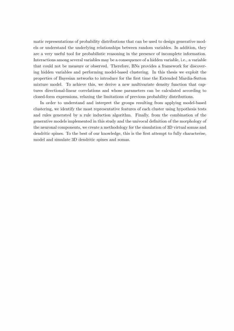
matic representations of probability distributions that can be used to design generative mod-
els or understand the underlying relationships between random variables. In addition, they
are a very useful tool for probabilistic reasoning in the presence of incomplete information.
Interactions among several variables may be a consequence of a hidden variable, i.e., a variable
that could not be measure or observed. Therefore, BNs provides a framework for discover-
ing hidden variables and performing model-based clustering. In this thesis we exploit the
properties of Bayesian networks to introduce for the first time the Extended Mardia-Sutton
mixture model. To achieve this, we derive a new multivariate density function that cap-
tures directional-linear correlations and whose parameters can be calculated according to
closed-form expressions, relaxing the limitations of previous probability distributions.
In order to understand and interpret the groups resulting from applying model-based
clustering, we identify the most representative features of each cluster using hypothesis tests
and rules generated by a rule induction algorithm. Finally, from the combination of the
generative models implemented in this study and the univocal definition of the morphology of
the neuronal components, we create a methodology for the simulation of 3D virtual somas and
dendritic spines. To the best of our knowledge, this is the first attempt to fully characterise,
model and simulate 3D dendritic spines and somas.

Resumen
Uno de los mayores desafıos a los que se enfrenta la ciencia actual es el de desentranar
el funcionamiento del cerebro, siendo la simulacion de los circuitos neuronales del cerebro
humano a diferentes escalas un area de estudio que ha despertado muchas expectativas e
interes. Dada la increıble complejidad de este objetivo, los modelos matematicos asistidos
por ordenador son una herramienta imprescindible para poder razonar, hacer predicciones y
sugerir nuevas hipotesis acerca del funcionamiento y organizacion de las neuronas. En esta
tesis nos centramos en el estudio de la morfologıa de las espinas dendrıticas y de somas de
neuronas piramidales humanas desde el punto de vista de la neuroanatomıa computacional.
Las espinas dendrıticas son pequenas protusiones membranosas situadas en la superficie de
las dendritas, siendo las encargadas de recibir las sinapsis excitatorias. Su morfologıa ha sido
asociada con funciones cognitivas tales como el aprendizaje o la memoria, y no es de extranar
que una gran variedad de enfermedades mentales se hayan relacionado con alteraciones en
su morfologıa o densidad. Por ello resulta de interes identificar las clases de espinas. La
categorizacion mas aceptada es la de Kaiserman-Abramof que propone cuatro grupos de
espinas, aunque se discute si la diversidad de morfologıas refleja mas un continuo que la
existencia de grupos concretos. Por su parte, los somas contienen el nucleo de la neurona
y son los encargados de generar los neurotransmisores, elementos basicos de las sinapsis y
por lo tanto de la actividad cerebral. Su morfologıa ha sido identificada como una de las
propiedades fundamentales para distinguir entre tipos de neuronas.
Para el desarrollo de esta disertacion utilizamos reconstrucciones individuales 3D de es-
pinas dendrticas y somas. La aplicacion de una novedosa tecnica de extraccion de atributos
nos permite caracterizar unıvocamente la geometrıa de estos cuerpos 3D de acuerdo a varias
magnitudes y direcciones. Mediante un analisis separamos de manera automatica y objetiva
las observaciones en categorıas homogeneas. Concretamente, aplicamos el clustering basado
en modelos, un enfoque probabilıstico que asume que los datos fueron generados por un mod-
elo estadıstico de mixturas y cuyo objetivo es ajustar dicho modelo a partir de los datos
observados. En este marco de trabajo cada grupo se representa con una distribucion de
probabilidad multidimensional. En el caso que nos ocupa, el aprendizaje de estos modelos de
acuerdo a la estadıstica clasica presenta serios problemas debido a su incapacidad para mane-
jar la periodicidad de los datos direccionales. En la literatura sobre estadıstica direccional
se han propuesto algunas distribuciones enfocadas a modelar los datos direccionales-lineales,
pero todas ellas exhiben importantes limitaciones para llevar a cabo clustering basado en
modelos. La mayorıa de las distribuciones direccionales-lineales se basan en copulas para
construir distribuciones bivariantes. Las distribuciones basadas en copulas presentan resulta-
dos teoricos complejos, lo que dificulta extenderlas a mas dimensiones. Ademas, la estimacion
de parametros de estas distribuciones requiere de algoritmos de optimizacion, cuya inclusion
al proceso de clustering puede ser prohibitivamente costosa desde una perspectiva computa-
cional. El clustering de datos multivariantes direccionales-lineales es aun mas desafiante y
practicamente se limita a modelos que asumen independencia entre variables direccionales y
lineales, lo que reduce gravemente la expresividad del modelo e introduce un numero innece-
sario de grupos.
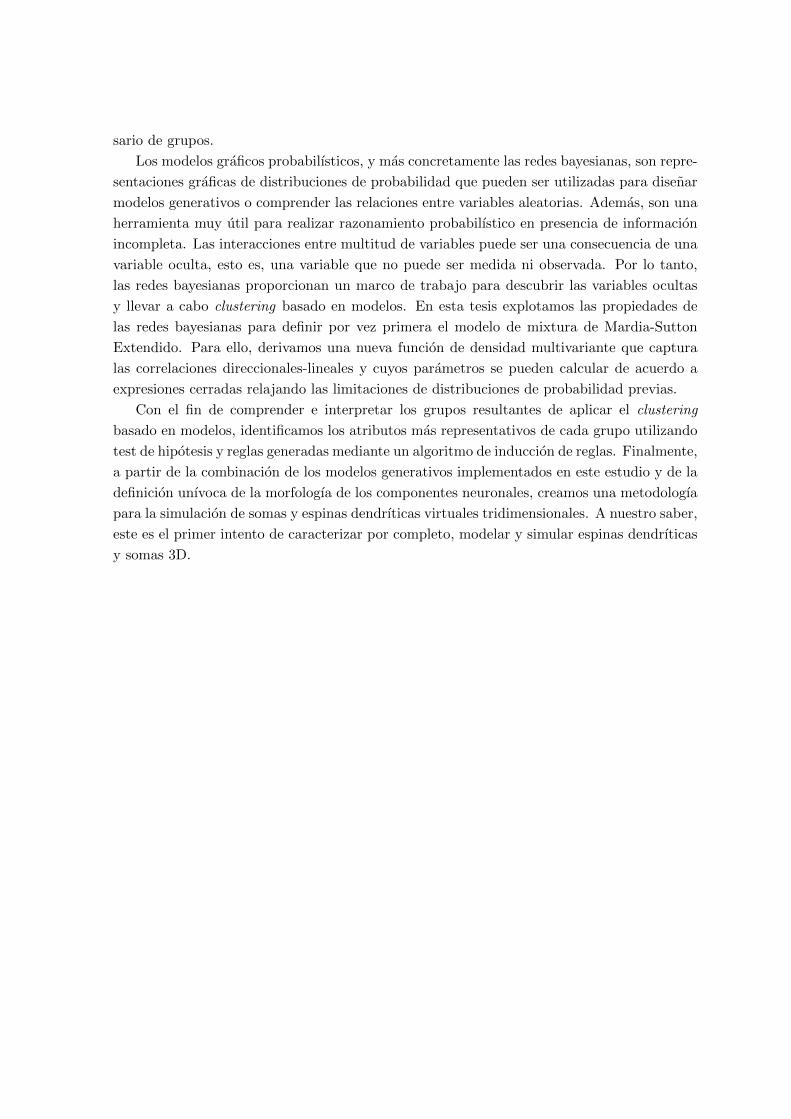
Los modelos graficos probabilısticos, y mas concretamente las redes bayesianas, son repre-
sentaciones graficas de distribuciones de probabilidad que pueden ser utilizadas para disenar
modelos generativos o comprender las relaciones entre variables aleatorias. Ademas, son una
herramienta muy util para realizar razonamiento probabilıstico en presencia de informacion
incompleta. Las interacciones entre multitud de variables puede ser una consecuencia de una
variable oculta, esto es, una variable que no puede ser medida ni observada. Por lo tanto,
las redes bayesianas proporcionan un marco de trabajo para descubrir las variables ocultas
y llevar a cabo clustering basado en modelos. En esta tesis explotamos las propiedades de
las redes bayesianas para definir por vez primera el modelo de mixtura de Mardia-Sutton
Extendido. Para ello, derivamos una nueva funcion de densidad multivariante que captura
las correlaciones direccionales-lineales y cuyos parametros se pueden calcular de acuerdo a
expresiones cerradas relajando las limitaciones de distribuciones de probabilidad previas.
Con el fin de comprender e interpretar los grupos resultantes de aplicar el clustering
basado en modelos, identificamos los atributos mas representativos de cada grupo utilizando
test de hipotesis y reglas generadas mediante un algoritmo de induccion de reglas. Finalmente,
a partir de la combinacion de los modelos generativos implementados en este estudio y de la
definicion unıvoca de la morfologıa de los componentes neuronales, creamos una metodologıa
para la simulacion de somas y espinas dendrıticas virtuales tridimensionales. A nuestro saber,
este es el primer intento de caracterizar por completo, modelar y simular espinas dendrıticas
y somas 3D.
Contents
Contents xv
List of Figures xviii
Acronyms xxi
I INTRODUCTION 1
1 Introduction 3
1.1 Hypotheses and objectives . . . . . . . . . . . . . . . . . . . . . . . . . . . . . 5
1.2 Document organization . . . . . . . . . . . . . . . . . . . . . . . . . . . . . . 6
II BACKGROUND 9
2 Model-based clustering with Bayesian networks 11
2.1 Introduction . . . . . . . . . . . . . . . . . . . . . . . . . . . . . . . . . . . . . 11
2.2 Probabilistic graphical models . . . . . . . . . . . . . . . . . . . . . . . . . . . 12
2.3 Notation and terminology . . . . . . . . . . . . . . . . . . . . . . . . . . . . . 12
2.4 Bayesian networks . . . . . . . . . . . . . . . . . . . . . . . . . . . . . . . . . 13
2.4.1 Inference . . . . . . . . . . . . . . . . . . . . . . . . . . . . . . . . . . 14
2.4.2 Structure learning . . . . . . . . . . . . . . . . . . . . . . . . . . . . . 15
2.4.3 Parameterisation . . . . . . . . . . . . . . . . . . . . . . . . . . . . . . 18
2.5 Model-based clustering . . . . . . . . . . . . . . . . . . . . . . . . . . . . . . . 23
3 Directional statistics 25
3.1 Introduction . . . . . . . . . . . . . . . . . . . . . . . . . . . . . . . . . . . . . 25
3.2 Directional probability distributions . . . . . . . . . . . . . . . . . . . . . . . 25
3.2.1 The von Mises distribution . . . . . . . . . . . . . . . . . . . . . . . . 28
3.3 Directional probabilistic graphical models . . . . . . . . . . . . . . . . . . . . 28
3.3.1 Spherical distributions . . . . . . . . . . . . . . . . . . . . . . . . . . . 29
3.3.2 Toroidal distributions . . . . . . . . . . . . . . . . . . . . . . . . . . . 30
3.3.3 Cylindrical distributions . . . . . . . . . . . . . . . . . . . . . . . . . . 31
xiii
xiv CONTENTS
3.4 Model-based clustering of directional-linear data . . . . . . . . . . . . . . . . 32
4 Neuroscience 35
4.1 Introduction . . . . . . . . . . . . . . . . . . . . . . . . . . . . . . . . . . . . . 35
4.2 Pyramidal neurons . . . . . . . . . . . . . . . . . . . . . . . . . . . . . . . . . 37
4.2.1 Neuronal soma . . . . . . . . . . . . . . . . . . . . . . . . . . . . . . . 38
4.2.2 Dendrites . . . . . . . . . . . . . . . . . . . . . . . . . . . . . . . . . . 39
4.2.3 Dendritic spines . . . . . . . . . . . . . . . . . . . . . . . . . . . . . . 39
4.3 Computational neuroanatomy . . . . . . . . . . . . . . . . . . . . . . . . . . . 42
4.3.1 Simulation of neuronal components . . . . . . . . . . . . . . . . . . . . 43
4.3.2 Bayesian networks in neuroanatomy . . . . . . . . . . . . . . . . . . . 44
III CONTRIBUTIONS TO DIRECTIONAL STATISTICS AND DATA
CLUSTERING 45
5 Directional-linear Bayesian networks for clustering 47
5.1 Introduction . . . . . . . . . . . . . . . . . . . . . . . . . . . . . . . . . . . . . 47
5.2 Naıve Bayes von Mises mixture model . . . . . . . . . . . . . . . . . . . . . . 48
5.2.1 Kullback-Leibler divergence and Bhattacharyya distance . . . . . . . . 50
5.2.2 Experiments . . . . . . . . . . . . . . . . . . . . . . . . . . . . . . . . 52
5.3 Hybrid Gaussian-von Mises mixture model . . . . . . . . . . . . . . . . . . . . 53
5.3.1 Kullback-Leibler divergence and Bhattacharyya distance . . . . . . . . 57
5.3.2 Experiments . . . . . . . . . . . . . . . . . . . . . . . . . . . . . . . . 58
5.4 Extended Mardia-Sutton mixture model based on Bayesian networks . . . . . 61
5.4.1 Kullback-Leibler divergence . . . . . . . . . . . . . . . . . . . . . . . . 63
5.4.2 Experiments . . . . . . . . . . . . . . . . . . . . . . . . . . . . . . . . 64
5.5 Conclusions . . . . . . . . . . . . . . . . . . . . . . . . . . . . . . . . . . . . . 66
IV CONTRIBUTIONS TO NEUROSCIENCE 69
6 3D morphology-based clustering and simulation of human pyramidal cell
dendritic spines 71
6.1 Introduction . . . . . . . . . . . . . . . . . . . . . . . . . . . . . . . . . . . . . 71
6.2 Preprocessing . . . . . . . . . . . . . . . . . . . . . . . . . . . . . . . . . . . . 72
6.2.1 Repairing spines . . . . . . . . . . . . . . . . . . . . . . . . . . . . . . 72
6.2.2 Feature extraction . . . . . . . . . . . . . . . . . . . . . . . . . . . . . 76
6.3 Clustering . . . . . . . . . . . . . . . . . . . . . . . . . . . . . . . . . . . . . . 79
6.3.1 Cluster interpretation and visualization . . . . . . . . . . . . . . . . . 79
6.3.2 Distribution of clusters by dendritic compartment, age and distance
from soma . . . . . . . . . . . . . . . . . . . . . . . . . . . . . . . . . . 83
6.3.3 Directional-linear clustering of dendritic spines . . . . . . . . . . . . . 86
CONTENTS xv
6.4 Simulation . . . . . . . . . . . . . . . . . . . . . . . . . . . . . . . . . . . . . . 87
6.5 Conclusions . . . . . . . . . . . . . . . . . . . . . . . . . . . . . . . . . . . . . 88
7 Univocal definition and clustering of neuronal somas 93
7.1 Introduction . . . . . . . . . . . . . . . . . . . . . . . . . . . . . . . . . . . . . 93
7.2 Preprocessing . . . . . . . . . . . . . . . . . . . . . . . . . . . . . . . . . . . . 94
7.2.1 Repairing the soma . . . . . . . . . . . . . . . . . . . . . . . . . . . . . 94
7.2.2 Automatic soma segmentation . . . . . . . . . . . . . . . . . . . . . . 98
7.2.3 Mesh comparison . . . . . . . . . . . . . . . . . . . . . . . . . . . . . . 100
7.2.4 Validation of automatic segmentation . . . . . . . . . . . . . . . . . . 101
7.2.5 Intra-expert variability . . . . . . . . . . . . . . . . . . . . . . . . . . . 103
7.2.6 Feature extraction . . . . . . . . . . . . . . . . . . . . . . . . . . . . . 105
7.3 Clustering . . . . . . . . . . . . . . . . . . . . . . . . . . . . . . . . . . . . . . 106
7.4 Simulation . . . . . . . . . . . . . . . . . . . . . . . . . . . . . . . . . . . . . . 112
7.5 Conclusions . . . . . . . . . . . . . . . . . . . . . . . . . . . . . . . . . . . . . 112
V CONCLUSIONS AND FUTURE WORK 115
8 Conclusions and future work 117
8.1 Summary of contributions . . . . . . . . . . . . . . . . . . . . . . . . . . . . . 117
8.2 List of publications . . . . . . . . . . . . . . . . . . . . . . . . . . . . . . . . . 118
8.3 Software . . . . . . . . . . . . . . . . . . . . . . . . . . . . . . . . . . . . . . . 119
8.4 Future work . . . . . . . . . . . . . . . . . . . . . . . . . . . . . . . . . . . . . 120
VI APPENDICES 123
A Set of rules for the characterization of dendritic spine clusters 125
B Proofs 127
B.1 Derivation of the Extended Mardia-Sutton distribution . . . . . . . . . . . . . 127
B.2 Bhattacharyya distance for the von Mises distribution . . . . . . . . . . . . . 130
B.3 Kullback-Leibler divergence for the von Mises distribution . . . . . . . . . . . 131
B.4 Kullback-Leibler divergence for the Extended Mardia-Sutton distribution . . 133
B.4.1 Conditional Kullback-Leibler divergence of the Extended Mardia-Sutton
distribution . . . . . . . . . . . . . . . . . . . . . . . . . . . . . . . . . 133
Bibliography 136

xvi CONTENTS
List of Figures
2.1 Structure of a naıve Bayes model GNB . . . . . . . . . . . . . . . . . . . . . . 14
3.1 Comparison among circular distributions . . . . . . . . . . . . . . . . . . . . 27
3.2 Examples of geometric spaces obtained from multivariate directional distri-
butions . . . . . . . . . . . . . . . . . . . . . . . . . . . . . . . . . . . . . . . 29
4.1 Graphical representation of a neuron . . . . . . . . . . . . . . . . . . . . . . 36
4.2 Major subdivisions of the brain . . . . . . . . . . . . . . . . . . . . . . . . . . 37
4.3 Pyramidal neuron . . . . . . . . . . . . . . . . . . . . . . . . . . . . . . . . . 38
4.4 Traditional classification of dendritic spines . . . . . . . . . . . . . . . . . . . 41
5.1 Graphical structure G for the naıve Bayes model when all the variables are
directional . . . . . . . . . . . . . . . . . . . . . . . . . . . . . . . . . . . . . 49
5.2 An example of the graphical structure G for the hybrid Gaussian-von Mises
model . . . . . . . . . . . . . . . . . . . . . . . . . . . . . . . . . . . . . . . . 55
5.3 Original structure of the Bayesian network learnt the by hybrid Gaussian-von
Mises model . . . . . . . . . . . . . . . . . . . . . . . . . . . . . . . . . . . . 59
5.4 An example of a Bayesian network structure representing a mixture of Ex-
tended Mardia-Sutton distributions . . . . . . . . . . . . . . . . . . . . . . . 62
6.1 3D reconstructions of human dendritic spines . . . . . . . . . . . . . . . . . . 74
6.2 Spine repair process and multiresolutional Reeb graph computation . . . . . 75
6.3 Spine features description . . . . . . . . . . . . . . . . . . . . . . . . . . . . . 78
6.4 Model-based clustering representation and interpretation of the morphology
of dendritic spines . . . . . . . . . . . . . . . . . . . . . . . . . . . . . . . . . 80
6.5 Graphical representations of the main features that characterise each cluster
of spines . . . . . . . . . . . . . . . . . . . . . . . . . . . . . . . . . . . . . . 82
6.6 Bar charts showing the distribution of spines belonging to each of the six
clusters according to the maximum membership probability p∗ . . . . . . . . 85
6.7 Examples of spines for each cluster discovered by the hybrid Gaussian-von
Mises mixture model . . . . . . . . . . . . . . . . . . . . . . . . . . . . . . . 87
6.8 Simulation of 3D dendritic spines . . . . . . . . . . . . . . . . . . . . . . . . 89
xvii
xviii LIST OF FIGURES
7.1 Repair and segmentation process of neural somas . . . . . . . . . . . . . . . 95
7.2 Example of 2D ambient occlusion . . . . . . . . . . . . . . . . . . . . . . . . 96
7.3 Mesh reconstruction . . . . . . . . . . . . . . . . . . . . . . . . . . . . . . . . 97
7.4 Example of shape diameter function . . . . . . . . . . . . . . . . . . . . . . . 98
7.5 Histogram after performing clustering for segmenting the soma . . . . . . . . 99
7.6 Examples of final soma result . . . . . . . . . . . . . . . . . . . . . . . . . . . 100
7.7 RMSE before and after repairing the experts’ somata . . . . . . . . . . . . . 102
7.8 Illustration of the goodness of the soma segmentation method on four cells . 103
7.9 RMSE between the somata extracted from six neurons by both experts on
three different days . . . . . . . . . . . . . . . . . . . . . . . . . . . . . . . . 104
7.10 Somata with their primary dendrites after manual segmentation . . . . . . . 105
7.11 Characterisation of the soma morphology . . . . . . . . . . . . . . . . . . . . 107
7.12 Feature extraction from the multiresolutional Reeb graph representation . . 108
7.13 The BN structure learned by the SEM algorithm during the clustering pro-
cess. To avoid cluttering the BN with many arcs, all the arcs from the latent
variable Z (top) to each variable are represented as only one arc from Z to the
group (inside the box). The BN structure shows that linear variables (green)
are interrelated in consecutive regions, such as |Br4| → |Br
3| → |Br2|. Also,
curvature variables θ and Θ (orange) are mostly correlated with directional
variables or other curvature variables. . . . . . . . . . . . . . . . . . . . . . . 109
7.14 Examples of somas attributed to their most probable cluster . . . . . . . . . 111
7.15 Simulation of virtual somas . . . . . . . . . . . . . . . . . . . . . . . . . . . . 113
List of Tables
3.1 Summary of works involving clustering of directional-linear data with their
limitations . . . . . . . . . . . . . . . . . . . . . . . . . . . . . . . . . . . . . 33
5.1 Comparison of parameter estimation between von Mises and Gaussian mixture
models changing the sample size . . . . . . . . . . . . . . . . . . . . . . . . . 52
5.2 Hit rate of von Mises vs Gaussian mixture models . . . . . . . . . . . . . . . 53
5.3 Parameter estimation of hybrid Gaussian-von Mises model with respect to the
original model . . . . . . . . . . . . . . . . . . . . . . . . . . . . . . . . . . . 60
5.4 Hit rate of hybrid Gaussian-von Mises and Gaussian mixture models . . . . . 60
5.5 Results for the Paired Wilcoxon signed-rank test checking if there were sig-
nificant differences between Extended Mardia-Sutton model and the hybrid
Gaussian-von Mises model . . . . . . . . . . . . . . . . . . . . . . . . . . . . 66
5.6 Comparison of the mean results obtained by the Extended Mardia-Sutton
model and the hybrid Gaussian-von Mises model. . . . . . . . . . . . . . . . 68
6.1 Number and percentage of spines after repair by their dendritic compartment
and age . . . . . . . . . . . . . . . . . . . . . . . . . . . . . . . . . . . . . . . 73
6.2 Number of spines whose maximum probability p∗ of belonging to a cluster is
greater than a threshold . . . . . . . . . . . . . . . . . . . . . . . . . . . . . . 79
6.3 Probability of misclassifying a spine from cluster P in cluster Q . . . . . . . 83
6.4 Results for Pearson’s χ2 test checking if the distribution of each cluster is
independent of its dendritic compartment, age and combination of both . . . 86
6.5 Number of dendritic spines as a function of their distance from the soma . . 86
7.1 Results from the Welch t-test and the Watson-Williams test, which checked
for significant differences between the means of the cluster and the rest of the
clusters . . . . . . . . . . . . . . . . . . . . . . . . . . . . . . . . . . . . . . . 110
xix

xx LIST OF TABLES
Acronyms
BD Bhattacharyya distance
BIC Bayesian information criterion
BN Bayesian network
CPT Conditional probability table
DAG Directed acyclic graph
EM Expectation Maximisation
EMS Extended Mardia-Shutton
HBP Human Brain Project
j.p.d. Joint probability distribution
LY Lucifer Yellow
MLE Maximum likelihood estimation
NB Naıve Bayes
p.d.f. Probability density function
SDF Shape diameter function
SEM Structural Expectation Maximisation
vM von Mises
xxi


Part I
INTRODUCTION
1


Chapter 1Introduction
The modern scientific investigation of the structure and mechanisms ruling the functionality
of the nervous system spans more than a century ago when Golgi invented the Golgi’s method
to stain nervous tissue and Ramon y Cajal proposed the neuron doctrine [Ramon y Cajal,
1904]. These findings provided the ground for a series of fundamental discoveries about
synaptic transmission, passive and active electric conductance, neurotrophic factors, etc.,
that have shaped the neuroscience as a highly interdisciplinary field [Ascoli, 2002] giving rise
to ambitious projects as the Cajal Blue Brain Project1, Human Brain Project2 or the BRAIN
initiative3. Their goal is to unravel the inner workings of the human mind and, in this way,
be able to deepen the study of numerous neurological and pathological diseases.
Computational neuroscience emerges as a consequence of the incredible complexity of the
brain to construct compact representations of neurobiological processes through computer-
assisted models, and to simulate the structure of the nervous system to different scales. This
research field provides the tools to address the question of how nervous systems operate on
the basis of known anatomy, physiology and circuitry [Dayan and Abbott, 2001]. In this
thesis we focus on computational neuroanatomy, that consists of the study of the shape and
structure of the nervous system, to characterise quantitatively the 3D morphology of the
neuronal soma and the dendritic spines of pyramidal neurons.
The pyramidal neurons, which receive that name because of the shape of their soma, were
discovered by Ramon y Cajal. They are the most abundant neurons in the cerebral cortex
and have been related to advanced cognitive functions. The soma is the component of the
neuron where its cell nucleus is placed. It is one of the fundamental components of the cell
for discriminating between different types of neurons [Svoboda, 2011]. The dendritic spines
are small membranous protrusions placed on the surface of some neuronal dendrites that are
the targets of most excitatory synapses in the cerebral cortex [Nimchinsky et al., 2002]. They
have captured the attention of neuroscientists since their morphology has been associated with
brain funcionality and disturbances as schizophrenia, dementia or mental retardation [Jacobs
1http://cajalbbp.cesvima.upm.es/2https://www.humanbrainproject.eu/en/3https://www.braininitiative.nih.gov/
3
4 CHAPTER 1. INTRODUCTION
et al., 1997]. Therefore the automatic characterisation, clustering and simulation of somas
and dendritic spines according to their morphology is of attracting interest in neuroscience
to reason and suggest new hypotheses about their functions.
Defining neuronal components through 3D morphological attributes is the first step for
an effective association between their shape and their functionality, the categorisation of a
neuron or to obtain accurate and complete simulations of neurons. Morphometric analysis
has been widely applied in neuroscience to quantitatively describe dendrite arborizations [As-
coli and Krichmar, 2000; Ascoli et al., 2001; Lopez-Cruz et al., 2011], somas [Alavi et al.,
2009; Meijering, 2010] or dendritic spines [Basu et al., 2018; Rodriguez et al., 2008]. Fre-
quently, the morphological characterisation of neurons requires the measure of directions and
magnitudes [Leguey et al., 2016; Lopez-Cruz et al., 2011]. After collecting these data an
exploratory analysis is usually performed to reveal patterns. A popular statistical tool to
accomplish this task is cluster analysis, i.e., data division into homogeneous groups describ-
ing their main characteristics. A probabilistic approach is model-based clustering [Fraley and
Raftery, 2002; McLachlan and Basford, 1988; Melnykov and Maitra, 2010] which assumes that
the data are generated by an underlying mixture of probability distributions. Finite mix-
ture models [McLachlan and Peel, 2000] provide a formal setting for model-based clustering
where each cluster is represented by a distribution. The most well-known method for prob-
abilistic clustering is the Gaussian mixture model [Titterington et al., 1985] which is widely
applied because of its computational tractability and its suitability to approximate any linear
multivariate density (variables defined on the domain (−∞,∞)) given enough components.
However, Gaussian mixture models are not able of handling periodicity of directional data
and consequently, they generally underperform in these datasets [Roy et al., 2016].
Directional statistics is the subdiscipline of statistics that deals with angles and rota-
tions representing observations as n-dimensional unit vectors [Jammalamadaka and Sengupta,
2001; Ley and Verdebout, 2017; Mardia and Jupp, 1999]. The study of a plethora of phenom-
ena requires the measure of directions and magnitudes as for example the wind speed and
direction in meteorology [Carta et al., 2008; Leguey, 2018], the acrophases for human natal-
ity in rhythmometry, medicine and demography [Batschelet et al., 1973; Batschelet, 1981],
or the hue and chroma in image recognition [Roy et al., 2016, 2017]. Mixtures of circular
[Jammalamadaka and Sengupta, 2001; Mardia and Jupp, 1999], spherical [Banerjee et al.,
2005] and toroidal [Mardia et al., 2008] probability distributions have been successfully ap-
plied in problems such as text categorisation, gene expression analysis and characterisation of
the structure of proteins improving models based on linear distributions. Nevertheless, clus-
tering of joint directional-linear data with parametric models is challenging because of the
lack of efficient density estimation methods and identifiability problems [Mastrantonio et al.,
2015]. These difficulties motivate that the literature about clustering directional-linear data
is limited to bivariate probability density functions or models that impose strong conditional
independence assumptions between the random variables involved.
Bayesian networks (BNs) [Koller and Friedman, 2009; Pearl, 1988] are probabilistic graph-
ical models that provide a compact and self-explanatory representation of multidimensional
1.1. HYPOTHESES AND OBJECTIVES 5
probability distributions. A BN comprises two components. The first component is the
structure, a directed acyclic graph that encodes conditional independences among triplets of
variables in the network. The second component is the set of parameters, i.e., the conditional
probability distributions of each variable given its parents in the graph. BNs are generative
models that effectively handle uncertainty and incomplete data [Pena et al., 1999; Pham and
Ruz, 2009]. The expectation-maximization (EM) algorithm [Dempster et al., 1977; McLach-
lan and Krishnan, 2008] is the most widely used algorithm for learning a model in the presence
of missing values. Friedman’s structural EM (SEM) algorithm [Friedman, 1997] extends the
EM algorithm to simultaneously learn the structure and parameters of a BN from incomplete
data. This method has been succesfully applied in semi-supervised classification [Hernandez-
Gonzalez et al., 2013; Wang et al., 2014] and clustering [Pena et al., 2000] problems. Given
the suitability of BNs to explicitly encode the conditional independence constraints between
variables through its structure, BNs has been applied in the context of classifying directional
[Lopez-Cruz et al., 2013] and directional-linear data [Leguey et al., 2016].
In this dissertation we pursue the study of the morphology of the soma and dendritic spines
from the point of view of computational neuroscience. To characterise the geometries of these
neuronal components we used individual 3D reconstructions of somas and dendritic spines
from human cortical pyramidal neurons. We propose a morphometric analysis procedure
based on 3D mesh processing and machine learning techniques to unambiguously capture the
shape of these components through a set of features describing their geometry. As result
we obtain magnitudes and directions. To deal with this data, we introduce mixture models
represented as BNs whose mixture components are directional-linear probability distributions.
The proposed mixture models allow us to perform model-based clustering with the aim of
uncover groups of somas and groups of dendritic spines based on their morphology and
analyse the differences between the groups. To better understand the differences between
the clusters, each soma and dendritic spine was crisply assigned to its most probable cluster.
Then, a rule-based classifying algorithm was applied to learn the discriminative characteristics
of each group. Furthermore, the resulting models allow to simulate 3D virtual representations
of somas and dendritic spines that match the morphological definitions of each cluster.
Chapter outline
The main hypothesis and objectives of this thesis are introduced in Section 1.1. In Section
1.2 we summarize and briefly describe the organization of the manuscript.
1.1 Hypotheses and objectives
The research hypotheses of this dissertation can be stated as the following two main points:
� The BNs in combination with the SEM algorithm can be applied to perform model-
based clustering on directional-linear data according to closed-form equations. The
resulting model can capture directional-linear interactions.

6 CHAPTER 1. INTRODUCTION
� The combination of an unambiguous characterisation of the morphology of neuronal
components with the generative models learned during the clustering process can be
used to simulate accurate 3D representations of somas and dendritic spines.
Based on these hypotheses, the main objectives of this dissertation are:
� To exploit BNs encoding of conditional independences for developing a multivariate
directional-linear joint probability distribution.
� To derive the closed-form expressions for the above multivariate probability distribution
in the context of the SEM algorithm.
� To define a methodology for objectively discovering and establishing groups of 3D neu-
ronal components based on their morphology, and for simulating realistic virtual repre-
sentation of somas and dendritic spines. This goal can be decomposed into the following
subgoals:
– To pre-process the 3D reconstructions of the neuronal components with the aim
of repairing artifacts introduced in their surface during the data acquisition and
unambiguously describe their geometry according to a set of features.
– To cluster the neuronal components and to identify the most prominent charac-
teristics of each group.
– To simulate virtual 3D neuronal components.
� To implement a software solution for the above methods and techniques.
1.2 Document organization
The manuscript includes six parts and eight chapters, organised as follows:
Part I. Introduction
This part introduces this dissertation.
- Chapter 1 summarises the hypotheses and objectives as well as the manuscript organi-
sation.
Part II. Background
This part consists of three chapters that introduce the basic and theoretical concepts applied
throughout this thesis. We discuss the literature of each topic within its corresponding
chapter.
- Chapter 2 introduces probabilistic graphical models as a compact framework for statis-
tical modelling under uncertainty, focusing on BNs and their properties. In this chapter
1.2. DOCUMENT ORGANIZATION 7
we examine different BN parameterisations that depend on the domain of the dataset
and we describe algorithms for performing inference and learning. We also address
model-based clustering by presenting the SEM algorithm.
- Chapter 3 presents the most widely used univariate distributions of directional statistics
paying special attention to the von Mises distribution. We discuss the extension of
these distributions to the multivariate case (in the sphere, torus and cylinder) and their
representations as probabilistic graphical models. Finally, we summarise the different
approaches proposed in the literature for model-based clustering of directional-linear
data.
- Chapter 4 provides a brief introduction to neuroscience focused primarily on pyramidal
neurons and some of their components, i.e., neuronal soma, dendrites, and dendritic
spines. Additionally, we present computational neuroanatomy examining its scope and
the research based on the simulation of neuronal components and BNs applied to neu-
roscience.
Part III. Contributions to directional statistics and data clustering
This part includes one chapter that presents our proposal in directional-linear data clustering
with BNs.
- Chapter 5 shows three finite mixture models for clustering multivariate directional and
directional-linear data where the predictor variables are assumed to follow the von
Mises (for directional data) and the Gaussian (for linear data) distributions. These are
the naıve Bayes von Mises, the hybrid Gaussian-von Mises and the Extended Mardia-
Sutton mixture models. We derive the closed-form expressions for these distributions
and for the SEM algorithm of the three models. Additionally, we provide the closed-
form equations for the Kullback-Leibler divergence and the Bhattacharyya distance to
evaluate the quality of the clusters. Experiments evaluating the performance of the
models are included.
Part IV. Contributions to neuroscience
This part includes two chapters that present our proposals in neuroscience related to dendritic
spines and neuronal somas.
- Chapter 6 deals with the pre-processing, clustering and simulation of the 3D reconstruc-
tions of dendritic spines from human pyramidal cells. Here, we design techniques to
repair the surface of the 3D dendritic spine representations and extract a set of features
that unambiguously represent the morphology of the spine according to their multires-
olutional Reeb graph representation. We use over 7,000 dendritic spine reconstructions
to perform model-based clustering according to a Gaussian mixture model and we anal-
yse the resulting groups in terms of their distributions by dendritic compartment, age,

8 CHAPTER 1. INTRODUCTION
distance from soma and we also find their most discriminative characteristics relying
on the rules generated by a rule induction algorithm. Then, we repeat the experiment
applying the hybrid Gaussian-von Mises and analyse the clusters discovered by this
model. From the resulting Gaussian mixture model we define a method to simulate 3D
virtual dendritic spines from each group.
- Chapter 7 presents an automatic reparation and segmentation method to delimit the
morphology of the neuronal soma. We validated the goodness of this automatic segmen-
tation method against manual segmentation by neuroanatomists to set up a framework
for comparison. From the set of segmented somas we characterise the morphology of
39 3D reconstructed human pyramidal somas in terms of their multiresolutional Reeb
graph representation, from which we extract a set of directional and linear variables
to perform model-based clustering. We deal with this dataset using the Extended
Mardia-Sutton mixture model. We perform Weltch t-tests, Watson-Williams tests, and
rule-based algorithms to characterise each group by its most prominent features. Fur-
thermore, the resulting model allows us to simulate 3D virtual representations of somas
from each cluster.
Part V. Conclusions and future work
This part concludes the dissertation.
- Chapter 8 summarises the contributions of this thesis and discusses future research
lines. Furthermore, we include the list of publications and software tools developed as
result of this research.
Part VI. Appendices
This part provides supplementary information about the research.
- Appendix A includes the rules generated by the RIPPER algorithm to characterise the
cluster of dendritic spines.
- Appendix B presents the derivations for the Kullback-Leibler and the Bhattacharyya
distance between two von Mises distributions, as well as the Kullback-Leibler divergence
between two Extended Mardia-Sutton distributions.

Part II
BACKGROUND
9

Chapter 2Model-based clustering with
Bayesian networks
2.1 Introduction
Uncertainty is an inherent property of most real-world problems. It is a consequence of diverse
factors as for example partial or incomplete information about a system or errors introduced
by measuring instruments. Probability theory provides a well-established foundation for
managing uncertainty and provides the mechanisms to reason and reach conclusions from
the available information [Sucar, 2015]. We could then describe and formulate uncertainty
through probabilistic models. We find that probabilistic graphical models [Castillo et al.,
1996; Koller and Friedman, 2009; Wainwright and Jordan, 2008] provide some advantages
over other probabilistic models as they are a diagrammatic representation of the probability
distributions that can be applied to design the models or to achieve a deeper understanding of
the relation among random variables. This acquires special relevance when it comes to analyse
complex systems that involve multiple interdependences between their components, as the
brain [Rubinov and Sporns, 2010]. In neuroscience it is crucial to identify and comprehend
these relations to uncover functional associations. Interactions among several variables may
be consequence of a hidden variable, i.e., a variable that could not be measured or observed
[Elidan et al., 2001]. Model based clustering [Fraley and Raftery, 2002; McLachlan and
Basford, 1988; Melnykov and Maitra, 2010] and its formalisation, the finite mixture model
[McLachlan and Peel, 2000], provides a framework for discovering hidden variables from a
given set of data points to obtain categories of points that share similar statistical properties.
In this dissertation we apply probabilistic graphical models and more concretely BNs
[Koller and Friedman, 2009; Koski and Noble, 2009; Neapolitan, 2004; Pearl, 1988] to perform
model-based clustering as they are suitable tools to capture the dependencies among variables
while it learns the underlying probability distribution.
11
12 CHAPTER 2. MODEL-BASED CLUSTERING WITH BAYESIAN NETWORKS
Chapter outline
Section 2.2 introduces probabilistic graphical models as a compact framework for proba-
bilistic modeling. Section 2.3 defines some useful notation and terminology. Section 2.4
discusses BNs in detail presenting inference, structure learning algorithms and several pa-
rameterisations. Probabilistic clustering through model-based clustering and the structural
expectation-maximisation algorithm are explained in Section 2.5.
2.2 Probabilistic graphical models
In the presence of uncertainty, the study of most complex systems requires to reason proba-
bilistically about their possible states. Given a set of random variables describing the system
the joint probability distribution (j.p.d.) represents all the possible states of the system and
assigns a probability to each of them [Dechter, 2013]. In the era of big data the number of
variables involved in the description of the system could be of thousands or even millions.
As the number of combinations grow exponentially with the number of variables, storing the
j.p.d. in the computer memory is not longer feasible even for a small number of variables.
Another limitation is that learning the j.p.d. may require huge amount of data to estimate
the probabilities robustly.
Probabilistic graphical models are a graph-based representation that provides a compact
and unifying framework for capturing conditional dependencies among random variables and
constructing multivariate probabilistic models. The graph or structure of a graphical model
consists of a set of nodes representing the random variables and a set of edges that corresponds
to probabilistic relations between those variables. The j.p.d. factorises according to the
structure as a product of factors, preventing the combinatorial blow up by exploiting the
independence properties of the distribution to reduce the dimension of the factors.
There are two main families of probabilistic graphical models. (i) Markov networks [Kin-
dermann and Snell, 1980; Rue and Held, 2005], also known as Markov random fields, are
undirected graphical models that have been successfully applied to image analysis and spa-
tial statistics [Cressie and Wikle, 2015; Li, 2009] and (ii) BNs that are the directed counter-
part. We focus on the latter because they provide a natural representation for many types
of real-world domains [Koller and Friedman, 2009].
2.3 Notation and terminology
We start introducing some basic terminology and notation that will be of common use along
the document:
� Variables names, such as X,Y, Z, are denoted by capital letters and their specific values
with lowercase letters x, y, z. Sets of variables are denoted by boldface capital letters
X,Y,Z and their instantiations are denoted by boldface lowercase letters x,y, z.
2.4. BAYESIAN NETWORKS 13
� We denote the dataset as D = {x1, ...,xN} where N is the number of instances and
xi = (xi1, xi2, ..., x
iL),∀i = 1, ..., N where L is the number of variables.
� The graph G = (V, E) is the structure of the BN. It consists of two components: the col-
lection of vertices or nodes V that corresponds to a given set of linear random variables
X = {X1, X2, ..., XL}, and the collection of arcs or edges E ⊂ V × V.
� We denote the parameters of the model as θ.
� The log-likelihood function of a BN B for a given dataset D is represented as `(B|D).
� Each arc in E consists of a pair of ordered nodes Xl → Xl+1 that indicates a direction.
For an arc Xl → Xl+1, we denote Xl+1 as the child of Xl, or conversely, Xl is the parent
of Xl+1. We use ChGXl and PaGXl = {U1l, U2l, ..., UT l} to denote the set of children and
parent nodes for node Xl in G respectively, where each variable Utl is one of the parents
of Xl and T is the number of parents of Xl. The set of parents of a set of variables is
defined as PaGX = {PaGX1,PaGX2
, ...,PaGXL}. Additionally, we say that Xl is an ancestor
of Xl+1 and Xl+1 is a descendant of Xl if there is a sequence of arcs Xl → · · · → Xl+1.
� For a given structure G, the Markov blanket of a node Xl in G is the set of nodes
composed of PaGXl , ChGXl and PaGChGXl
.
� A directed acyclic graph is a graph where there are not direct cycles. A directed cycle
is a sequence of arcs X1 → X2 → · · · → Xl → Xl+1 ∈ E such that X1 = Xl+1.
� An ordering of the nodes X1, ..., XL is a topological ordering for G if, whenever we have
Xl → Xl+1 ∈ E , then l < l + 1. As a result, all the nodes are ordered such that the
parents come before their children.
2.4 Bayesian networks
A BN [Koller and Friedman, 2009; Koski and Noble, 2009; Murphy, 2012; Neapolitan, 2004;
Pearl, 1988] B is a directed acyclic graph that represents the probabilistic relationships among
a given set of random variables X. A BN consists of a pair of components B = (G,θ), where
G is the structure, and θ are the parameters of the model. Structure G encodes conditional
independences among triplets of variables in the network. The set of parameters θ comprises
the conditional probability distribution of each variable given its parents in G. The BNs
satisfy the local Markov property, i.e., each variable is independent of its non-descendants
given its parents in the graph. Hence, the j.p.d. factorises as
p(X;θ) =L∏l=1
p(Xl|PaGXl ;θ). (2.1)
As discussed in Section 2.2, this is a compact representation of the j.p.d., reducing the
dimensionality of the factors and consequently the amount of parameters to be estimated.
14 CHAPTER 2. MODEL-BASED CLUSTERING WITH BAYESIAN NETWORKS
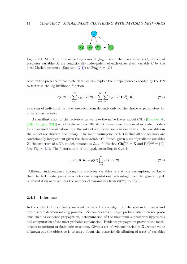
Figure 2.1: Structure of a naıve Bayes model GNB. Given the class variable C, the set ofpredictor variables X are conditionally independent of each other given variable C by thelocal Markov property (Equation (2.1)) as PaGNBX = {C}
Also, in the presence of complete data, we can exploit the independences encoded by the BN
to factorise the log-likelihood function
`(B|D) =N∑i=1
log p(xi|θ) =N∑i=1
L∑l=1
log p(xil|PaGXl ,θ), (2.2)
as a sum of individual terms where each term depends only on the choice of parameters for
a particular variable.
As an illustration of the factorisation we take the naıve Bayes model (NB) [Duda et al.,
2001; Murphy, 2012] which is the simplest BN structure and one of the most extended models
for supervised classification. For the sake of simplicity, we consider that all the variables in
the model are discrete and binary. The main assumption of NB is that all the features are
conditionally independent given the class variable C. Hence, given a set of predictor variables
X, the structure of a NB model, denoted as GNB, fulfils that ChGNBC = X and PaGNBX = {C}(see Figure 2.1). The factorisation of the j.p.d. according to GNB is
p(C,X;θ) = p(C)
L∏l=1
p(Xl|C;θ). (2.3)
Although independence among the predictor variables is a strong assumption, we know
that the NB model provides a notorious computational advantage over the general j.p.d.
representation as it reduces the number of parameters from O(2L) to O(L).
2.4.1 Inference
In the context of uncertainty we want to extract knowledge from the system to reason and
optimise the decision making process. BNs can address multiple probabilistic inference prob-
lems such as evidence propagation, determination of the maximum a posteriori hypothesis
and computation of the most probable explanation. Evidence propagation provides the mech-
anisms to perform probabilistic reasoning. Given a set of evidence variables Xe whose value
is known xe, the objective is to query about the posterior distribution of a set of variables
2.4. BAYESIAN NETWORKS 15
whose value is unknown Xq. Therefore, the evidence propagation computation is
p(Xq|Xe;θ) =p(Xq,Xe;θ)
p(Xe;θ).
Basically, conditioning consists of clamping the evidence variables to their values xe and then
normalising to go from p(Xq,Xe;θ) to p(Xq|Xe;θ).
Inference methods are divided into two main groups: exact and approximate (see Salmeron
et al. [2018] for a recent review). The former consists of calculating, through a set of algebraic
operations (sums and products), the probability distribution of interest. Most of the exact
methods are based on variable elimination [Dechter, 2013; Shachter, 1990; Zhang and Poole,
1994], recursive conditioning [Darwiche, 2001; Pearl, 1985], or junction tree belief propagation
[Jensen et al., 1990; Shenoy and Shafer, 1990] algorithms. However, inference is generally
NP-hard [Cooper, 1990] and exact inference algorithms can become unfeasible to apply for
complex BNs. Approximate inference methods are an alternative solution based on con-
structing an approximation to the target distribution usually based on statistical sampling
techniques. The most widely applied approximation algorithms are based on belief prop-
agation [Minka, 2001; Pearl, 1988; Welling and Teh, 2001], variational methods [Jaakkola
and Qi, 2007; Jordan et al., 1999], Markov Chain Monte Carlo methods [Gilks et al., 1996;
MacKay, 1998; Neal, 1993] or particle filtering [Bidyuk and Dechter, 2007; Doucet et al.,
2000] algorithms.
2.4.2 Structure learning
The purpose of generative models is to discover the probability distribution from which the
dataset D was generated. In the case under examination, we assume that the dataset D come
from the BN B∗ = (G∗,θ∗) which is unknown. Clearly, our goal during the learning process
is to recover B∗. Since in this section we are interested specifically on the structure, we focus
on techniques to recover G∗.
Sometimes, both the structure and the parameters of the network can be elucidated from
the knowledge of experts. However, it can be laborious and expensive or even impossible
in large applications. Therefore, automatic techniques are needed that allow learning G∗
from D. Unfortunately, this goal is hard to achieve mainly because data are noisy and we
cannot be certain about the underlying distribution. Another limitation is that the space
of possible structures has a super-exponential cardinality on the number of nodes V (see
Robinson [1977]). For this reason, structure learning has received much attention with the
aim of improving the learning techniques giving rise to three different approaches: constraint-
based methods, methods based on maximisation of a score criterion and hybrid methods which
combines both constraint-based and maximisation of a score criterion techniques (see Daly
et al. [2011] for an extensive review).
16 CHAPTER 2. MODEL-BASED CLUSTERING WITH BAYESIAN NETWORKS
2.4.2.1 Constraint-based structure learning
Each BN structure corresponds to a set of probability distributions that it can represent.
Then, an equivalence class of BNs is defined by all the BN structures that represent the same
set of distributions. The constraint-based techniques provide a framework for learning the
equivalence class of BNs that best explain dependencies and independencies on D using con-
ditional independence tests under the faithfulness assumption, i.e., when graphical separation
and probabilistic conditional independence imply each other.
Algorithms for constraint-based learning consist of two steps [Scutari, 2017]:
1. It learns the skeleton of the graph checking through conditional independence tests if
there is a set of variables that separates a particular pair of nodes. If that set is empty,
then there must be an edge between the pair of nodes.
2. It tries to assign directions to the edges of the graph by using some rules [Meek, 1995].
Some arcs can be undirected because sometimes both directions are equivalent providing
the same decomposition of the j.p.d. As a result, the constraint-based algorithms
return completed partially directed acyclic graphs which represent an equivalence class
containing multiple DAGs.
Some of the most celebrated constraint-based algorithms are the Inductive-Causation
[Verma and Pearl, 1991], the PC algorithm [Buhlmann et al., 2010; Kalisch and Buhlmann,
2007, 2008; Spirtes et al., 2000] which is the first practical implementation of the Inductive-
Causation algorithm, the Grow-Shrink algorithm [Bromberg et al., 2009; Margaritis, 2003]
or the Incremental Association Markov blanket [Tsamardinos et al., 2003; Yaramakala and
Margaritis, 2005]. For a more extended overview of the algorithms see [Koller and Friedman,
2009; Scutari and Denis, 2014]. The main drawback of these methods is that they can be
sensitive to failures in individual independence tests and if just one of these tests returns
a wrong answer it can mislead the network construction procedure. Other disadvantage is
that the amount of data required by these algorithms to have a sufficient large sample for
correctly identifying the conditional independences hugely increases with the cardinality of
the conditional set.
2.4.2.2 Score+search structure learning
The score+search-based BN learning can be approached as an optimisation problem [Gamez
et al., 2011; Tsamardinos et al., 2006] that depends on four terms: the hypothesis space, the
set of operators, the scoring function and the dataset D. The hypothesis space is the set of
candidate structures that are considered as potential solutions. The structure optimisation
procedure applies the set of operators to search over the set of candidate structures evaluating
how well they fit D according to the scoring function. Several heuristics have been proposed
in the literature to cope with the superexponential nature of the problem of searching for the
highest-scoring network structure. Depending on their nature they are usually grouped into:
2.4. BAYESIAN NETWORKS 17
� Order-based: They assume an initial topological order for the variables. Successive
changes are then applied to this order with the aim of optimising the network score.
Given a set of operators over the orders, changes can be made locally using greedy search
methods [Alonso-Barba et al., 2011; Cooper and Herskovits, 1992; Scanagatta et al.,
2017; Teyssier and Koller, 2005] or some metaheuristics [Faulkner, 2007; Hsu et al.,
2002; Larranaga et al., 1996]. Their main disadvantages are that, without restrictions,
there are as many orderings as permutations of variables, so the complexity in the worst
case scenario is O(L!), and also a bad order selection can produce graphs that are more
complex than it is needed for representing the probability distribution.
� Greedy search: These algorithms begin by choosing an initial structure G as the starting
point. The score of this structure is calculated for future comparisons. Then we get
all the neighbour networks of G in the space of hypotheses, i.e., all the legal networks
obtained by applying a single operator (e.g. arc addition, arc removal or arc reversion)
to G, and compute the score for each of them. Finally we replace G by the network
that obtained the best score during the procedure. This is repeated iteratively until
there are not changes in the structure that improve the score. The most basic form of
this technique is the greedy-hill climbing method [Chickering et al., 1996; Heckerman
et al., 1995]. A variant of this method applies the branch and bound [Miguel and Shen,
2001; Suzuki, 1999, 2018] technique, which is an exact method to reduce the hypothesis
space, speeding-up the learning procedure.
� Metaheuristics: Over the last decades techniques such as genetic algorithms [Holland,
1992], estimation of distribution algorithms [Larranaga and Lozano, 2001], genetic pro-
gramming [Koza and Koza, 1992], simulated annealing [Kirkpatrick et al., 1983] or tabu
search [Bouckaert, 1995; Glover et al., 1993] have been widely applied because of their
ability to find good solutions for combinatorial problems in a reasonable time. Since
the search for the optimal structure is a problem with a huge hypothesis space, these
methods look like promising approaches. A common representation of a BN to search
in the space of possible DAGs is to use the connectivity matrix. Some works based on
this representation are Blanco et al. [2003]; Etxeberria et al. [1997]; Larranaga et al.
[1996b,a]; Wong et al. [1999]. As discussed above, metaheuristics can also be applied to
obtain good topological orders. An extended review about these methods can be found
in Larranaga et al. [2013].
Evaluating a structure according to any score function involves estimating the optimal
parameters for each network candidate. Computing the complete set of parameters of a model
(see Section 2.4.3) for every candidate structure can be extremely time consuming or even
infeasible. However, as we show in Section 2.4, in the presence of complete data, the log-
likelihood function (Equation (2.2)) factorises according to G in a sum of terms where each
term depends only on the choice of parameters for a particular variable. We can exploit that
to avoid redundant calculations and score each node locally. The log-likelihood is a measure
of the fitness of a model to the data but unfortunately it can run into overfitting problems
18 CHAPTER 2. MODEL-BASED CLUSTERING WITH BAYESIAN NETWORKS
given that it always prefers a complex network over a simpler one [Koller and Friedman, 2009].
Penalized scoring functions [McLachlan and Peel, 2000] try to overcome this problem adding
a penalisation term to the log-likelihood function. An example is the Bayesian information
criterion (BIC) [Schwarz, 1978] defined as
BIC(D,B) = `(B|D)− v log(N)
2, (2.4)
where v is the number of parameters in B and N is the number of instances in D. Other
scoring functions widely applied are Akaike information criterion [Akaike, 1974], Bayesian
Dirichlet for likelihood-equivalence [Heckerman et al., 1995] and K2 [Cooper and Herskovits,
1992]. Any of these scoring functions are susceptible to being applied for efficient learning as
both the log-likelihood and the penalization term decompose according to the structure.
Score+search methods evaluate the whole structure at once. Hence, they are more robust
against individual failures than constraint-based methods, balancing the degree of dependence
between variables with the cost of increasing the complexity of the model. Their main
drawback is that they pose a search problem that may not have an elegant and efficient
solution.
2.4.2.3 Hybrid structure learning
It is a combination of the two previous methods. The algorithms in this group are based on
two steps called restrict and maximise. In the first step the objective is to reduce the set
of candidate parents for each variable Xl selecting those that have some relation with Xl.
This is intended to reduce the hypothesis space. The second step consists of a score+search
optimisation subject to the restrictions imposed by the first step.
Any of the techniques described for constraint-based and score+search structure learning
can be applied to the restrict and maximise steps respectively. However, some combinations
make more sense than others. The most representative algorithms of this group are the Sparse
Candidate [Friedman et al., 1999] and the Max-Min Hill-Climbing [Tsamardinos et al., 2006]
algorithms.
2.4.3 Parameterisation
As seen above, the marginals and the conditional probability distributions are the building
blocks of the BNs to construct complex j.p.d.s. Any approximator function can be used to
define these distributions, as for example logistic regressions [Lerner et al., 2001], kernel es-
timators [Hofmann and Tresp, 1996], neural networks [Choi and Darwiche, 2018; Monti and
Cooper, 1997], Gaussian processes [Friedman and Nachman, 2000], etc. However, most of
them present difficulties for efficient inference and learning. We examine three cases that are
particularly worthy of note because the parent-child relationship can be extended hierarchi-
cally to construct arbitrarily complex graphs. Depending on the nature of the dataset D we
distinguish between discrete, Gaussian and hybrid BNs.
2.4. BAYESIAN NETWORKS 19
2.4.3.1 Discrete Bayesian networks
In the discrete BNs [Darwiche, 2009] all the variables in X are defined in the categorical
domain. A natural choice to represent a finite number of states for a system is the cate-
gorical distribution. This distribution provides several advantages when modeling data, so
the assumption that data is distributed according to a categorical distribution is by far the
most common in the literature of BNs. One of its benefits is that it factorises in a product
of categorical distributions and, consequently, all the building blocks of the BN belong to
the same distribution thereby simplifying the computations. Also they provide transparency
given that the conditional probability distribution p(Xl|PaGXl ;θ) can be encoded in human-
readable tabular format known as a conditional probability table (CPT), which designates
a probability for every assignment of Xl and PaGXl . Additionally the interpretability of the
model is favored by the direct representation of the parameters as probabilities.
Maximum likelihood estimation (MLE) is the most common method for parameter esti-
mation in BNs. It is based on choosing the parameters θ that maximise the log-likelihood
(Equation (2.2)) for a given D. Hence, it is defined as
θ = argmaxθ
`(B|D). (2.5)
As the log-likelihood function of the j.p.d. factorises according to the BN structure in the
presence of complete data, learning or updating the parameters can be performed efficiently
as each CPT can be estimated locally. For the CPT p(Xl|PaGXl ;θ), the MLE is computed
according to
θlmj =Nlmj∑j Nlmj
, (2.6)
where Nlmj is the counts in D such that Xl = j and PaGXl = m and Nm is the number of
instances where PaGXl = m.
Given the desirable properties of discrete BNs discussed above and the simplicity of the
calculations in the estimation of the parameters, it is natural to bin continuous variables into
a finite set of intervals. Discretisation can be performed manually by a human expert [Chen
and Pollino, 2012], automatically using the response variable (if any) to optimise the cutoffs
and the number of the intervals [Dougherty et al., 1995; Fayyad and Irani, 1993], or using the
distribution of the continuous variables to ensure that the discretisation procedure introduces
enough intervals to capture the interactions between adjacent variables in the structure of the
BN [Friedman and Goldszmidt, 1996]. It is still an unsolved problem and different strategies
can be applied depending on the data [Beuzen et al., 2018; Nojavan et al., 2017]. The
main drawback of discretisation is that it only captures rough characteristics of the original
continuous distribution of the data and its application can lead to the loss of information from
the system influencing the accuracy of the model [Friedman and Goldszmidt, 1996]. Also,
the categorical representation of variables entails an exponential growth on the number of
parameters with respect to the number of parents, which limits the complexity of the models.
20 CHAPTER 2. MODEL-BASED CLUSTERING WITH BAYESIAN NETWORKS
2.4.3.2 Gaussian Bayesian networks
In the real-valued domain the most studied approach in BN modeling is based on the Gaussian
distribution [Geiger and Heckerman, 1994; Shachter and Kenley, 1989]. Gaussians are a
subclass of the exponential family distributions [Wainwright and Jordan, 2008] that make
very strong assumptions, such as symmetric exponential decay around the mean and linear
dependence among variables [Koller and Friedman, 2009]. These assumptions seem too strong
and do not hold in most of the cases. However, Gaussians provide a surprisingly good
approximation for many distributions. The explanation is that the Gaussian distribution is
the maximum entropy density function among all the real-valued distributions supported in
(−∞,∞) and, according to the principle of maximum entropy [Guiasu and Shenitzer, 1985;
Jaynes, 1957], without further information the distribution of maximum entropy is the one
that best represent the state of our knowledge.
The joint probability density function (p.d.f.) of the multivariate Gaussian distribution
is characterised according to two parameters, a mean vector µ and a symmetric covariance
matrix Σ. The expression for the multivariate Gaussian distribution is
fN (X;µ,Σ) =1
(2π)n/2|Σ|1/2e−
12
(X−µ)>Σ−1(X−µ). (2.7)
As we have discussed along this chapter, to properly factorise a distribution according to a
BN structure we have to define the marginal and the conditional density functions. It results
that both operations are very easy to perform for the multivariate Gaussian distribution.
Assume that we have a joint p.d.f. over X = {Xa,Xb} where Xa and Xb are two disjoint sets
of real-valued variables. Then, the parameters of the multivariate Gaussian can be decompose
as follows:
f
(Xa
Xb
)∼ fN
[(Xa
Xb
);
(µa
µb
),
(Σaa Σab
Σba Σbb
)].
According to this representation, marginalisation of a set of variable (e.g. Xb) in this form is
trivial as it can be directly read from the mean µb and the covariance Σbb. The definition of
the conditional probability distribution for a multivariate Gaussian is achieved through the
Schur complement decomposition [Zhang, 2005] which transforms the p.d.f. to
f
(Xa
Xb
)= f(Xb)f(Xa|Xb) = fN (Xb;µb,Σbb)fN (Xa;β0 + β>Xb,Q), (2.8)
where
β0 = µa −ΣabΣ−1bb µb,
β> = ΣabΣ−1bb ,
Q = Σaa −ΣabΣ−1bb Σba.
2.4. BAYESIAN NETWORKS 21
Several useful properties of the Gaussian emerge from this representation. First, both the
marginal and the conditional density functions are also Gaussian distributions. Therefore we
can apply marginalisation and conditioning iteratively in the resulting subsets of variables.
Second, the marginal distribution over Xb is explicitly represented in µb and Σbb so it can
be efficiently computed. The conditional distribution over Xa is a linear combination of
the variables in Xb. Finally, it provides a more compact representation than the discrete
representation given that the number of parameters increase quadratically in the number of
variables instead of exponentially.
As in Section 2.4.3.1, parameter estimation involves the maximization of sums of log-
likelihoods because of the factorisation represented by the BN structure (see Equation (2.2)).
Therefore, the parameters are estimated locally for each variable. For example, let us assume
that Xa = {Xl} in Equation (2.8) and PaGXl = {U1l, U2l, ..., UT l}. Then, by the local Markov
property (see Equation (2.1)) it is fulfilled that Xb = PaGXl . Consequently, for all variables
X \ PaGXl their regression coefficients are zero. The remaining regression coefficients β>l =
(β0l, β1l, ..., βT l), which corresponds to β in Equation (2.8) when Xa = {Xl} and are those
that belong to PaGXl , are estimated by solving the following system of equations
ED[Xl] = β0lED[1]+ β1lED[U1l]+· · ·+ βT lED[UT l] (2.9)
ED[Xl · U1l] = β0lED[U1l]+ β1lED[U1l · U1l]+· · ·+ βT lED[U1l · UT l]...
......
...
ED[Xl · UT l] =β0lED[UT l]+β1lED[U1l · UT l]+· · ·+ βT lED[UT l · UT l],
where each of the terms is an average value of the sample dataset ED[·], i.e., ED[1] =1N
∑Ni=1 1, ED[Xl] = 1
N
∑Ni=1 x
il, ED[Xl·Utl] = 1
N
∑Ni=1 x
il ·uitl and ED[Ujl·Utl] = 1
N
∑Ni=1 u
ij ·uitl.
Once the beta coefficients are known, the variance of Equation (2.8) Q = σ2l is computed as
σ2l =
∑Ni=1(xil − β0l −
∑Tt=1 βtlu
itl)
2
N. (2.10)
Note that when PaGXl = ∅ these expressions reduce to the well-known formulas for the sample
mean and the sample variance of the univariate Gaussian as ED[Xl] is the mean of Xl and
the system of equations becomes ED[Xl] = β0l; and σ2l =
∑Ni=1(xil−β0l)
2
N .
Gaussian distribution is well understood because of its linearity assumption among vari-
ables. Because of that, Gaussian BNs can be learned efficiently using closed-form expressions.
Nevertheless, this is a serious restriction that limits the expressive power of the model and
its application to domains with non-linear interactions. Although different approaches based
on learning with non-parametric densities [Hofmann and Tresp, 1996] or Gaussian process
networks [Friedman and Nachman, 2000] have been proposed in the literature to overcome
this problem, non-linear interactions between variables are usually represented as mixtures
22 CHAPTER 2. MODEL-BASED CLUSTERING WITH BAYESIAN NETWORKS
of Gaussians [Sung, 2003].
2.4.3.3 Hybrid Bayesian networks
Purely discrete or continuous datasets are unusual in complex real-world problems. Hybrid
BNs encompass both types of variables and define the basic operations to learn probabilistic
graphical models from these data. So far we have discussed the homogeneous relationships
between variables when all of them follow a categorical or a Gaussian distribution. The treat-
ment of the interactions among variables can be extrapolated to hybrid BNs when both the
parents and their children follow the same distribution and it is categorical or Gaussian. We
now turn our attention to incorporate the relations between discrete and continuous variables
to the model. More concretely, we have to study two types of dependencies: a continuous
variable with continuous and discrete parents, and a discrete variable with continuous and
discrete parents.
The simplest way to represent the first type of dependencies is to assume that the set
of parameters for the continuous variables changes as a consequence of the discrete parent
values. Let assume a set of categorical variables Z with K values or states for z and a set of
continuous variables X. The conditional distribution in hybrid BNs has the form
f(X|Z = k;θ) = f(X|Z;θk).
where θk are context-specific parameters for the instantiation z = k. Hence, for each instan-
tiation of z a density function is obtained. There is not restriction about f(X|Z;θk) which
can be any p.d.f. In the concrete case where the density function of X is Gaussian [Cobb and
Shenoy, 2006; Lauritzen, 1992; Lauritzen and Jensen, 2001], i.e., f(X|Z;θk) = fN (X;µk,Σk),
we can condition each Gaussian variable according to Equation (2.8) and in the presence of
complete data we can factorised the joint p.d.f. to efficiently compute the MLE with the
expressions provided in Equation (2.6) for Z, and Equation (2.9) and Equation (5.9) with
ED[Xl] =∑N
i=1 p(zi|xi;θk)xil.
Of special interest for the development of this thesis is the result induced from the
marginalisation over the discrete variables
f(X;θ) =
K∑k=1
p(Z;θk)f(X|Z;θk), (2.11)
which is the expression for a mixture model, where p(Z;θk) are the mixing weights that
are given by the probability of that instantiation and f(X|Z;θk) is the distribution for the
mixture component k. Among the mixture models, the Gaussian mixture model [Titterington
et al., 1985] is the most known because of its computational tractability and its suitability
to approximate any linear multivariate density given enough components. It is also widely
applied for model-based clustering.
Modeling the relationships between variables when a discrete variable has continuous
2.5. MODEL-BASED CLUSTERING 23
parents varies depending on the nature of the discrete variable. When the discrete variable
presents several categories or states and these are ordinal we can assume that the variable
follows a Gaussian distribution. If this is not the case, alternatively we can use a softmax
function to model the continuous-discrete interaction [Lerner et al., 2001; Murphy, 1999]
or define thresholds over the continuous variables to discretise them [Koller and Friedman,
2009]. The problem with these approaches is that inference becomes complex and usually it
is assumed that continuous variables cannot be parents of categorical variables.
2.5 Model-based clustering
Model-based clustering [Fraley and Raftery, 2002; McLachlan and Basford, 1988; Melnykov
and Maitra, 2010] is generally defined as a finite mixture of models [McLachlan and Peel,
2000] where each cluster represents a probability distribution. The convex combination of
the probability distributions generates the mixture density function (see Equation (2.11)).
In this context Z is assumed to be a set of hidden or latent variables which are categorical
variables and each of their states corresponds to a one mixture component. Hence, the result
of clustering is a probabilistic assignment of each instance to each cluster. Learning BNs for
clustering is a challenging task given that conditional independence assumptions encoded by
the local Markov property (Equation (2.1)) do not apply when Z is unobserved. Consequently,
scoring functions do not factorise and is not longer feasible to search for an optimal network
efficiently.
EM algorithm [Dempster et al., 1977; McLachlan and Krishnan, 2008] is the most widely
used algorithm for estimating the parameters of a model in the presence of incomplete data.
EM addresses the missing data problem by selecting a starting point, which is either an initial
set of parameters or an initial assignment to the latent variables Z. Once we have a parameter
set, we can apply inference to complete the data or, conversely, once we have the complete
data we can estimate the set of parameters from the MLE method. Thus, it is an iterative
method comprising two steps. The expectation step (E-step) completes Z probabilistically
according to
Qi(zi) = p(zi|xi;θ) =
f(xi|zi;θ)p(zi;θ)∑z f(xi|z;θ)p(z;θ)
, (2.12)
resulting in the completed dataset D+. The maximisation step (M-step) estimates a new set
of parameters from D+
θ = argmaxθ
N∑i=1
∑zi
Qi(zi) log
f(xi, zi;θ)
Qi(zi). (2.13)
The EM algorithm iterates between both steps improving the likelihood of the model for a
given D until convergence [Xu and Jordan, 1996].
In the BN case, the EM algorithm only optimises the parameters θ, assuming a predeter-
mined and fixed structure G. The SEM algorithm [Friedman, 1997] extends the EM algorithm
24 CHAPTER 2. MODEL-BASED CLUSTERING WITH BAYESIAN NETWORKS
including structural learning to simultaneously learn G and θ of a BN from incomplete data.
SEM starts with a specified initial structure and set of parameters. Then, it alternates be-
tween EM and structure optimisation. For a given G, EM algorithm estimates the parameters
θ according to the MLE method and infers the completed dataset D+ (Equation (2.12) and
Equation (2.13)). Once the data are complete, the model factorises according to the local
Markov property allowing efficient score+search structure learning. Both steps are repeated
iteratively until convergence. A common choice for the score to be maximised is the BIC
score (Equation (2.4)) because it avoids overfitting and, if the search procedure always finds
a better structure at each iteration, it is ensured the convergence of the EM algorithm.

Chapter 3Directional statistics
3.1 Introduction
In a wide range of scientific fields, angle measurement is required to represent information
about a phenomenon. Classical statistics is not suitable for modelling directional data because
it cannot handle periodicity. For example, given the angles 1° and 359°, the linear mean would
be 180°. This points in the opposite direction to the directional mean which is 0°. Thus,
models based on the Gaussianity assumption generally underperform in directional datasets
[Roy et al., 2016] and concrete methods to deal with directionality are required to take into
account the structure of this data. This chapter recaps directional statistics [Jammalamadaka
and Sengupta, 2001; Ley and Verdebout, 2017; Mardia, 1975b; Mardia and Jupp, 1999], the
branch of mathematics that provides the techniques and background to deal with directional
observations represented by unit vectors. We revise probabilistic graphical models in the
context of directional statistics and the representation of multivariate directional probability
distributions. Since directional data usually come along with their magnitude (linear data),
we also review the directional-linear literature and its application for data clustering.
Chapter outline
Section 3.2 introduces some procedures to construct circular distributions, discusses the most
widely used univariate distributions of directional statistics paying special attention to the von
Mises distribution. Section 3.3 presents multivariate directional distributions and their adap-
tation to develop probabilistic graphical models. Section 3.4 discusses different approaches
proposed in the literature for model-based clustering of directional-linear data.
3.2 Directional probability distributions
Directional statistics literature is prolific in probability distributions. Next, we describe some
general procedures to construct circular p.d.f., i.e., defined in the domain [0, 2π), and briefly
25
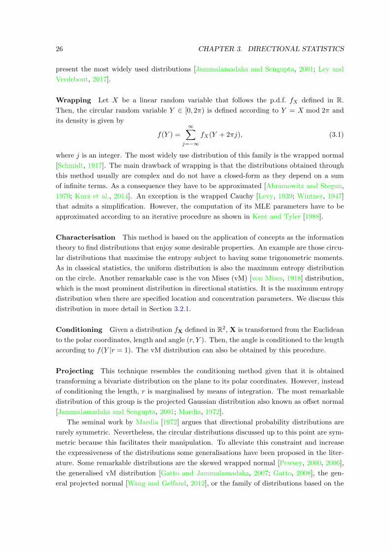
26 CHAPTER 3. DIRECTIONAL STATISTICS
present the most widely used distributions [Jammalamadaka and Sengupta, 2001; Ley and
Verdebout, 2017].
Wrapping Let X be a linear random variable that follows the p.d.f. fX defined in R.
Then, the circular random variable Y ∈ [0, 2π) is defined according to Y = X mod 2π and
its density is given by
f(Y ) =∞∑
j=−∞fX(Y + 2πj), (3.1)
where j is an integer. The most widely use distribution of this family is the wrapped normal
[Schmidt, 1917]. The main drawback of wrapping is that the distributions obtained through
this method usually are complex and do not have a closed-form as they depend on a sum
of infinite terms. As a consequence they have to be approximated [Abramowitz and Stegun,
1970; Kurz et al., 2014]. An exception is the wrapped Cauchy [Levy, 1939; Wintner, 1947]
that admits a simplification. However, the computation of its MLE parameters have to be
approximated according to an iterative procedure as shown in Kent and Tyler [1988].
Characterisation This method is based on the application of concepts as the information
theory to find distributions that enjoy some desirable properties. An example are those circu-
lar distributions that maximise the entropy subject to having some trigonometric moments.
As in classical statistics, the uniform distribution is also the maximum entropy distribution
on the circle. Another remarkable case is the von Mises (vM) [von Mises, 1918] distribution,
which is the most prominent distribution in directional statistics. It is the maximum entropy
distribution when there are specified location and concentration parameters. We discuss this
distribution in more detail in Section 3.2.1.
Conditioning Given a distribution fX defined in R2, X is transformed from the Euclidean
to the polar coordinates, length and angle (r, Y ). Then, the angle is conditioned to the length
according to f(Y |r = 1). The vM distribution can also be obtained by this procedure.
Projecting This technique resembles the conditioning method given that it is obtained
transforming a bivariate distribution on the plane to its polar coordinates. However, instead
of conditioning the length, r is marginalised by means of integration. The most remarkable
distribution of this group is the projected Gaussian distribution also known as offset normal
[Jammalamadaka and Sengupta, 2001; Mardia, 1972].
The seminal work by Mardia [1972] argues that directional probability distributions are
rarely symmetric. Nevertheless, the circular distributions discussed up to this point are sym-
metric because this facilitates their manipulation. To alleviate this constraint and increase
the expressiveness of the distributions some generalisations have been proposed in the liter-
ature. Some remarkable distributions are the skewed wrapped normal [Pewsey, 2000, 2006],
the generalised vM distribution [Gatto and Jammalamadaka, 2007; Gatto, 2008], the gen-
eral projected normal [Wang and Gelfand, 2012], or the family of distributions based on the
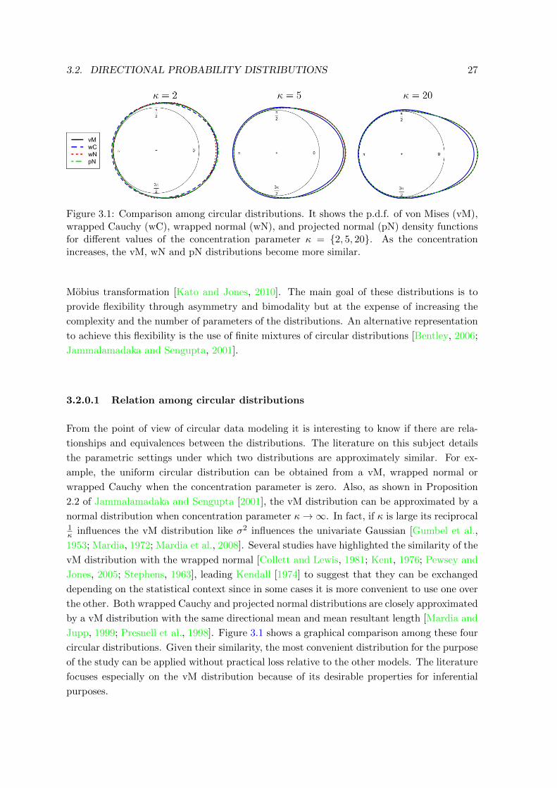
3.2. DIRECTIONAL PROBABILITY DISTRIBUTIONS 27
Figure 3.1: Comparison among circular distributions. It shows the p.d.f. of von Mises (vM),wrapped Cauchy (wC), wrapped normal (wN), and projected normal (pN) density functionsfor different values of the concentration parameter κ = {2, 5, 20}. As the concentrationincreases, the vM, wN and pN distributions become more similar.
Mobius transformation [Kato and Jones, 2010]. The main goal of these distributions is to
provide flexibility through asymmetry and bimodality but at the expense of increasing the
complexity and the number of parameters of the distributions. An alternative representation
to achieve this flexibility is the use of finite mixtures of circular distributions [Bentley, 2006;
Jammalamadaka and Sengupta, 2001].
3.2.0.1 Relation among circular distributions
From the point of view of circular data modeling it is interesting to know if there are rela-
tionships and equivalences between the distributions. The literature on this subject details
the parametric settings under which two distributions are approximately similar. For ex-
ample, the uniform circular distribution can be obtained from a vM, wrapped normal or
wrapped Cauchy when the concentration parameter is zero. Also, as shown in Proposition
2.2 of Jammalamadaka and Sengupta [2001], the vM distribution can be approximated by a
normal distribution when concentration parameter κ→∞. In fact, if κ is large its reciprocal1κ influences the vM distribution like σ2 influences the univariate Gaussian [Gumbel et al.,
1953; Mardia, 1972; Mardia et al., 2008]. Several studies have highlighted the similarity of the
vM distribution with the wrapped normal [Collett and Lewis, 1981; Kent, 1976; Pewsey and
Jones, 2005; Stephens, 1963], leading Kendall [1974] to suggest that they can be exchanged
depending on the statistical context since in some cases it is more convenient to use one over
the other. Both wrapped Cauchy and projected normal distributions are closely approximated
by a vM distribution with the same directional mean and mean resultant length [Mardia and
Jupp, 1999; Presnell et al., 1998]. Figure 3.1 shows a graphical comparison among these four
circular distributions. Given their similarity, the most convenient distribution for the purpose
of the study can be applied without practical loss relative to the other models. The literature
focuses especially on the vM distribution because of its desirable properties for inferential
purposes.
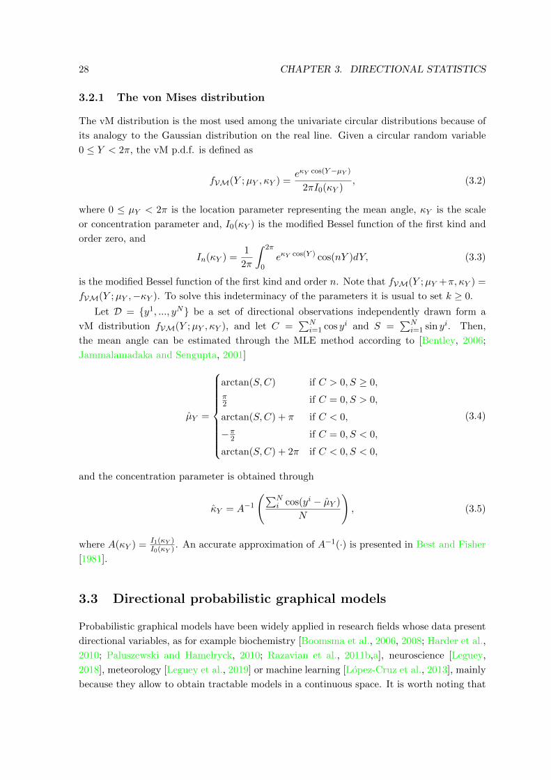
28 CHAPTER 3. DIRECTIONAL STATISTICS
3.2.1 The von Mises distribution
The vM distribution is the most used among the univariate circular distributions because of
its analogy to the Gaussian distribution on the real line. Given a circular random variable
0 ≤ Y < 2π, the vM p.d.f. is defined as
fVM(Y ;µY , κY ) =eκY cos(Y−µY )
2πI0(κY ), (3.2)
where 0 ≤ µY < 2π is the location parameter representing the mean angle, κY is the scale
or concentration parameter and, I0(κY ) is the modified Bessel function of the first kind and
order zero, and
In(κY ) =1
2π
∫ 2π
0eκY cos(Y ) cos(nY )dY, (3.3)
is the modified Bessel function of the first kind and order n. Note that fVM(Y ;µY +π, κY ) =
fVM(Y ;µY ,−κY ). To solve this indeterminacy of the parameters it is usual to set k ≥ 0.
Let D = {y1, ..., yN} be a set of directional observations independently drawn form a
vM distribution fVM(Y ;µY , κY ), and let C =∑N
i=1 cos yi and S =∑N
i=1 sin yi. Then,
the mean angle can be estimated through the MLE method according to [Bentley, 2006;
Jammalamadaka and Sengupta, 2001]
µY =
arctan(S,C) if C > 0, S ≥ 0,
π2 if C = 0, S > 0,
arctan(S,C) + π if C < 0,
−π2 if C = 0, S < 0,
arctan(S,C) + 2π if C < 0, S < 0,
(3.4)
and the concentration parameter is obtained through
κY = A−1
(∑Ni cos(yi − µY )
N
), (3.5)
where A(κY ) = I1(κY )I0(κY ) . An accurate approximation of A−1(·) is presented in Best and Fisher
[1981].
3.3 Directional probabilistic graphical models
Probabilistic graphical models have been widely applied in research fields whose data present
directional variables, as for example biochemistry [Boomsma et al., 2006, 2008; Harder et al.,
2010; Paluszewski and Hamelryck, 2010; Razavian et al., 2011b,a], neuroscience [Leguey,
2018], meteorology [Leguey et al., 2019] or machine learning [Lopez-Cruz et al., 2013], mainly
because they allow to obtain tractable models in a continuous space. It is worth noting that
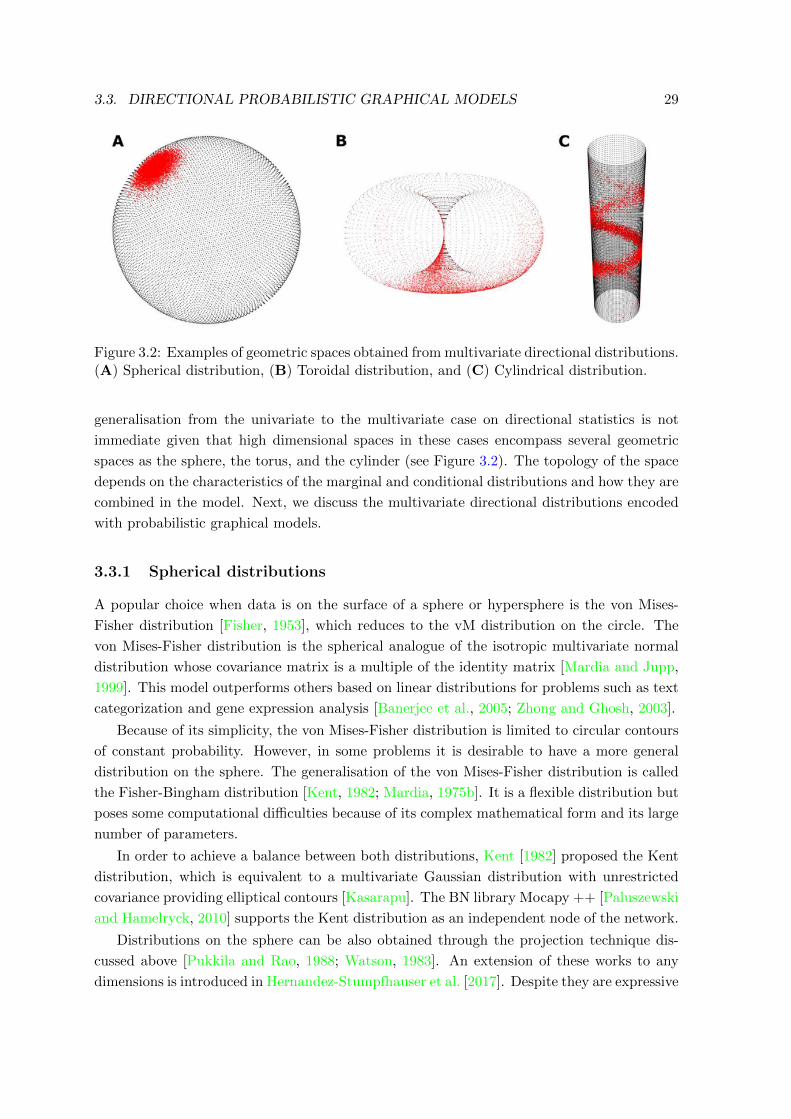
3.3. DIRECTIONAL PROBABILISTIC GRAPHICAL MODELS 29
Figure 3.2: Examples of geometric spaces obtained from multivariate directional distributions.(A) Spherical distribution, (B) Toroidal distribution, and (C) Cylindrical distribution.
generalisation from the univariate to the multivariate case on directional statistics is not
immediate given that high dimensional spaces in these cases encompass several geometric
spaces as the sphere, the torus, and the cylinder (see Figure 3.2). The topology of the space
depends on the characteristics of the marginal and conditional distributions and how they are
combined in the model. Next, we discuss the multivariate directional distributions encoded
with probabilistic graphical models.
3.3.1 Spherical distributions
A popular choice when data is on the surface of a sphere or hypersphere is the von Mises-
Fisher distribution [Fisher, 1953], which reduces to the vM distribution on the circle. The
von Mises-Fisher distribution is the spherical analogue of the isotropic multivariate normal
distribution whose covariance matrix is a multiple of the identity matrix [Mardia and Jupp,
1999]. This model outperforms others based on linear distributions for problems such as text
categorization and gene expression analysis [Banerjee et al., 2005; Zhong and Ghosh, 2003].
Because of its simplicity, the von Mises-Fisher distribution is limited to circular contours
of constant probability. However, in some problems it is desirable to have a more general
distribution on the sphere. The generalisation of the von Mises-Fisher distribution is called
the Fisher-Bingham distribution [Kent, 1982; Mardia, 1975b]. It is a flexible distribution but
poses some computational difficulties because of its complex mathematical form and its large
number of parameters.
In order to achieve a balance between both distributions, Kent [1982] proposed the Kent
distribution, which is equivalent to a multivariate Gaussian distribution with unrestricted
covariance providing elliptical contours [Kasarapu]. The BN library Mocapy ++ [Paluszewski
and Hamelryck, 2010] supports the Kent distribution as an independent node of the network.
Distributions on the sphere can be also obtained through the projection technique dis-
cussed above [Pukkila and Rao, 1988; Watson, 1983]. An extension of these works to any
dimensions is introduced in Hernandez-Stumpfhauser et al. [2017]. Despite they are expressive
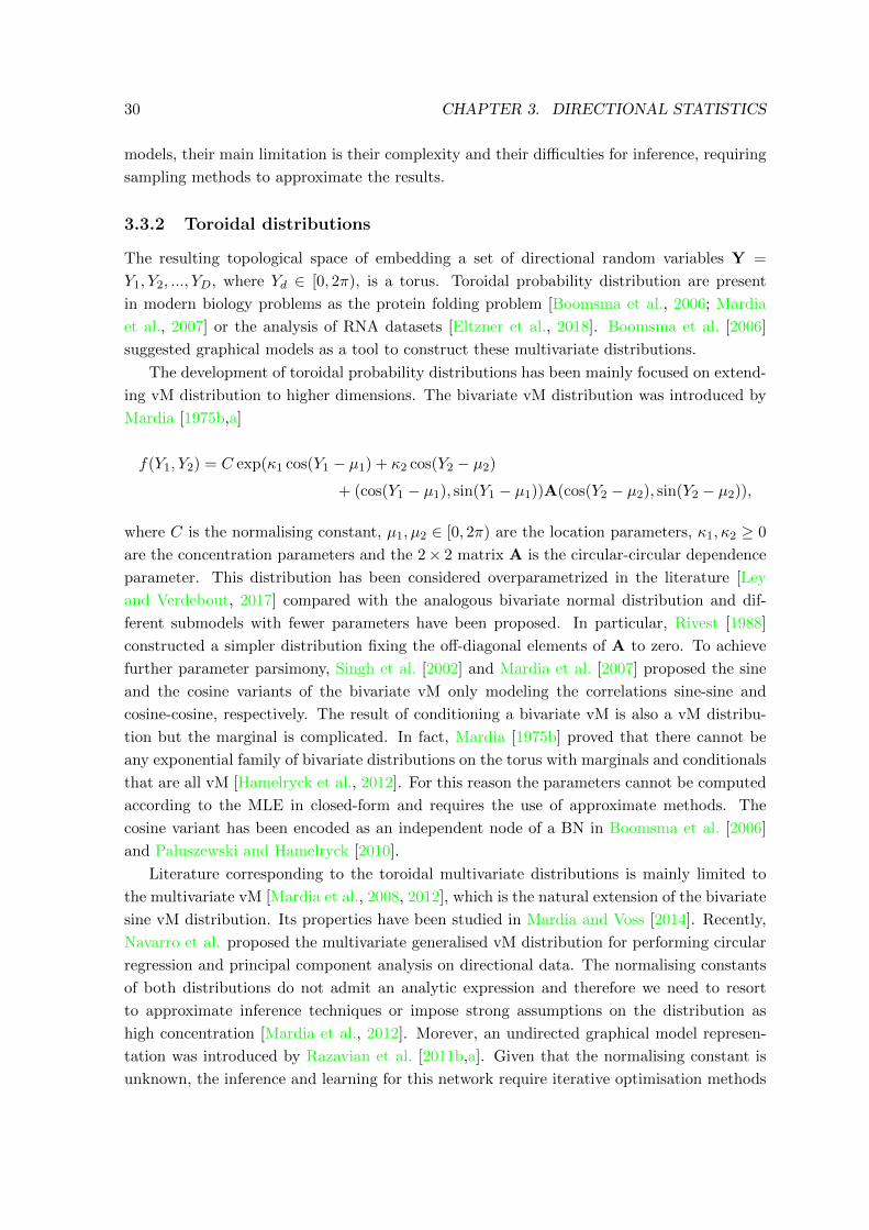
30 CHAPTER 3. DIRECTIONAL STATISTICS
models, their main limitation is their complexity and their difficulties for inference, requiring
sampling methods to approximate the results.
3.3.2 Toroidal distributions
The resulting topological space of embedding a set of directional random variables Y =
Y1, Y2, ..., YD, where Yd ∈ [0, 2π), is a torus. Toroidal probability distribution are present
in modern biology problems as the protein folding problem [Boomsma et al., 2006; Mardia
et al., 2007] or the analysis of RNA datasets [Eltzner et al., 2018]. Boomsma et al. [2006]
suggested graphical models as a tool to construct these multivariate distributions.
The development of toroidal probability distributions has been mainly focused on extend-
ing vM distribution to higher dimensions. The bivariate vM distribution was introduced by
Mardia [1975b,a]
f(Y1, Y2) = C exp(κ1 cos(Y1 − µ1) + κ2 cos(Y2 − µ2)
+ (cos(Y1 − µ1), sin(Y1 − µ1))A(cos(Y2 − µ2), sin(Y2 − µ2)),
where C is the normalising constant, µ1, µ2 ∈ [0, 2π) are the location parameters, κ1, κ2 ≥ 0
are the concentration parameters and the 2× 2 matrix A is the circular-circular dependence
parameter. This distribution has been considered overparametrized in the literature [Ley
and Verdebout, 2017] compared with the analogous bivariate normal distribution and dif-
ferent submodels with fewer parameters have been proposed. In particular, Rivest [1988]
constructed a simpler distribution fixing the off-diagonal elements of A to zero. To achieve
further parameter parsimony, Singh et al. [2002] and Mardia et al. [2007] proposed the sine
and the cosine variants of the bivariate vM only modeling the correlations sine-sine and
cosine-cosine, respectively. The result of conditioning a bivariate vM is also a vM distribu-
tion but the marginal is complicated. In fact, Mardia [1975b] proved that there cannot be
any exponential family of bivariate distributions on the torus with marginals and conditionals
that are all vM [Hamelryck et al., 2012]. For this reason the parameters cannot be computed
according to the MLE in closed-form and requires the use of approximate methods. The
cosine variant has been encoded as an independent node of a BN in Boomsma et al. [2006]
and Paluszewski and Hamelryck [2010].
Literature corresponding to the toroidal multivariate distributions is mainly limited to
the multivariate vM [Mardia et al., 2008, 2012], which is the natural extension of the bivariate
sine vM distribution. Its properties have been studied in Mardia and Voss [2014]. Recently,
Navarro et al. proposed the multivariate generalised vM distribution for performing circular
regression and principal component analysis on directional data. The normalising constants
of both distributions do not admit an analytic expression and therefore we need to resort
to approximate inference techniques or impose strong assumptions on the distribution as
high concentration [Mardia et al., 2012]. Morever, an undirected graphical model represen-
tation was introduced by Razavian et al. [2011b,a]. Given that the normalising constant is
unknown, the inference and learning for this network require iterative optimisation methods

3.3. DIRECTIONAL PROBABILISTIC GRAPHICAL MODELS 31
like Gibbs sampling [Bishop, 2006] and the computation of the pseudo-likelihood. Lopez-Cruz
et al. [2013] exploited the conditional independence assumptions encoded by the naıve Bayes
classifier to factorise the joint p.d.f. in a product of univariate vM enabling efficient model
learning.
Other multivariate toroidal distributions are the bivariate wrapped normal [Johnson and
Wehrly, 1978] and the multivariate wrapped normal [Baba, 1981] which have wrapped normals
as conditional and marginal distributions. However, they do not belong to the exponential
family and the estimation of the parameters even in the simplest cases leads to tough nu-
merical solutions that involve ratios of infinite sums, making the algorithms computationally
inefficient [Fisher and Lee, 1994].
3.3.3 Cylindrical distributions
The construction of a joint bivariate directional and linear p.d.f. is a non-trivial problem
being literature about directional-linear distributions scarce. Johnson and Wehrly [1978]
presented several cylindrical distributions invoking maximum entropy principles and a general
method based on copulas to construct bivariate cylindrical distributions with specified circular
and linear marginals. This method has inspired new cylindrical distributions that provide
tractability and flexibility [Abe and Ley, 2017; Kato and Shimizu, 2008] but suffer from
some drawbacks. Because of the complicated theoretical results, copulas are suitable for the
bivariate case but are difficult to extend to higher dimensions. Additionally, it is also arduous
to give closed-form expressions of the MLE equations for copulas.
Conditional probabilities in the cylinder have been proposed in the context of circular
regression models. Gould [1969] introduced a linear regression over the mean direction for
the case where the independent variable is linear and the response variable is directional.
This model presents identifiability problems because the likelihood has infinitely many dis-
tinct global maxima. Also, Fisher and Lee [1992] extended this work applying a monotone
function to the linear regression, mapping the domain (−∞,∞) to (−π, π). The likelihood
of this model is multimodal with maximum on a very narrow peak which can present severe
problems for numerical optimisation methods. Finally, Presnell et al. [1998] developed the
spherically projected multivariate linear model which uses the projection method to obtain
a directional distribution from a conditional Gaussian. Parameter estimation and inference
require iterative optimisation methods as the Newton-Raphson or the EM algorithm.
A different approach to define a bivariate cylindrical distribution was proposed by Mardia
and Sutton [1978] based on conditioning a trivariate Gaussian distribution with some restric-
tions on the parameters. Given the random variables X ∈ R and Y ∈ [0, 2π) they defined
the joint p.d.f. as
fMS(X,Y ;β, σ, µY , κY ) = fN (X;β0 + β1 cosY + β2 sinY, σ)fVM(Y ;µY , κY ) (3.6)
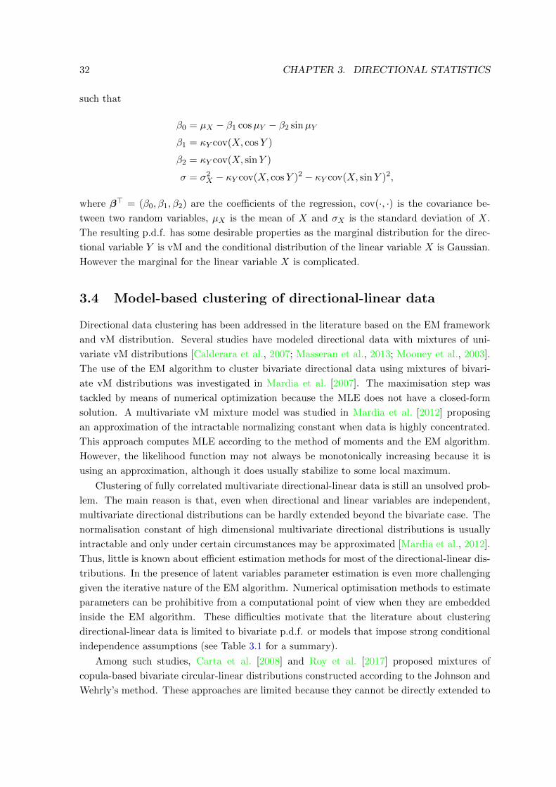
32 CHAPTER 3. DIRECTIONAL STATISTICS
such that
β0 = µX − β1 cosµY − β2 sinµY
β1 = κY cov(X, cosY )
β2 = κY cov(X, sinY )
σ = σ2X − κY cov(X, cosY )2 − κY cov(X, sinY )2,
where β> = (β0, β1, β2) are the coefficients of the regression, cov(·, ·) is the covariance be-
tween two random variables, µX is the mean of X and σX is the standard deviation of X.
The resulting p.d.f. has some desirable properties as the marginal distribution for the direc-
tional variable Y is vM and the conditional distribution of the linear variable X is Gaussian.
However the marginal for the linear variable X is complicated.
3.4 Model-based clustering of directional-linear data
Directional data clustering has been addressed in the literature based on the EM framework
and vM distribution. Several studies have modeled directional data with mixtures of uni-
variate vM distributions [Calderara et al., 2007; Masseran et al., 2013; Mooney et al., 2003].
The use of the EM algorithm to cluster bivariate directional data using mixtures of bivari-
ate vM distributions was investigated in Mardia et al. [2007]. The maximisation step was
tackled by means of numerical optimization because the MLE does not have a closed-form
solution. A multivariate vM mixture model was studied in Mardia et al. [2012] proposing
an approximation of the intractable normalizing constant when data is highly concentrated.
This approach computes MLE according to the method of moments and the EM algorithm.
However, the likelihood function may not always be monotonically increasing because it is
using an approximation, although it does usually stabilize to some local maximum.
Clustering of fully correlated multivariate directional-linear data is still an unsolved prob-
lem. The main reason is that, even when directional and linear variables are independent,
multivariate directional distributions can be hardly extended beyond the bivariate case. The
normalisation constant of high dimensional multivariate directional distributions is usually
intractable and only under certain circumstances may be approximated [Mardia et al., 2012].
Thus, little is known about efficient estimation methods for most of the directional-linear dis-
tributions. In the presence of latent variables parameter estimation is even more challenging
given the iterative nature of the EM algorithm. Numerical optimisation methods to estimate
parameters can be prohibitive from a computational point of view when they are embedded
inside the EM algorithm. These difficulties motivate that the literature about clustering
directional-linear data is limited to bivariate p.d.f. or models that impose strong conditional
independence assumptions (see Table 3.1 for a summary).
Among such studies, Carta et al. [2008] and Roy et al. [2017] proposed mixtures of
copula-based bivariate circular-linear distributions constructed according to the Johnson and
Wehrly’s method. These approaches are limited because they cannot be directly extended to

3.4. MODEL-BASED CLUSTERING OF DIRECTIONAL-LINEAR DATA 33
Reference X dim. Y dim. Limitations
Carta et al. [2008] 1 1 As a copula-based distribution, it cannotbe directly extended to higher dimensions
Roy et al. [2017] 1 1 As a copula-based distribution, it cannotbe directly extended to higher dimensions
Mastrantonio et al. [2015] 1 1 Only considers one circular variableLagona and Picone [2011] 1 1 Assume independence between a linear
and a circular variables given the latentvariable
Lagona et al. [2015] 1 1 Assume independence between a linearand a circular variables given the latentvariable
Lagona and Picone [2012] 2 2 Bivariate directional and bivariate skewednormal distributions are conditionally in-dependent given the latent variable
Bulla et al. [2012] 2 2 Bivariate directional and bivariate lineardistributions are conditionally indepen-dent given the latent variable
Roy et al. [2016] L 1 Full correlation among one circular andseveral linear variables
Table 3.1: Summary of works involving clustering of directional-linear data with their lim-itations. The columns named “X dim.” and “Y dim.” denote the maximum number oflinear and directional variables considered by each distribution, respectively. L refers to anundetermined number of linear variables.

34 CHAPTER 3. DIRECTIONAL STATISTICS
higher dimensions. Also in the bivariate circular-linear framework, Mastrantonio et al. [2015]
introduced a multivariate hidden Markov model to jointly cluster time-series of circular-linear
observations relying on the general projected normal distribution.
When it comes to generalise from cylindrical p.d.f. to higher dimensions, the simplest way
to model the component densities is to proceed on the basis that the directional and the linear
variables are independent of each other. For this setting, MLE can be computed efficiently
according to closed-form equations. Lagona and Picone [2011] and Lagona et al. [2015]
considered mixtures of independent univariate distributions to analyse meteorological data
and sea regimes. The main drawback of this approach is that these models can introduce
an unnecessary number of latent states given the lack of expressiveness of the underlying
mixture components.
Less restrictive models have been proposed in the literature allowing homogeneous cor-
relations (linear-linear or directional-directional) but assuming that directional and linear
variables are conditionally independent given the latent variable. Bulla et al. [2012] and Lag-
ona and Picone [2012] identified sea regimes by defining mixtures in which each component
is the product of a bivariate von Mises and a bivariate skewed normal that are conditionally
independent given the latent variable.
A joint p.d.f. for circular-linear data that incorporates correlations among a circular and
several linear variables was applied by Roy et al. [2016] for image segmentation. They de-
scribed colour images as mixtures of semi-wrapped Gaussians involving one wrapped normal
variable fully correlated with Gaussian variables. An extension of this model to consider
more than one circular variable leads to difficulties in parameter estimation as Roy et al.
have pointed out.

Chapter 4Neuroscience
4.1 Introduction
Unveiling the functioning of the brain is one of the main challenges faced by current science.
Neuroscientists seek to solve the unknowns and mysteries that have accompanied the brain
for centuries.
The study of the brain has its origin in the ancient world, in which doctors thought it
was composed of “phlegm”. Later, Aristotle considered that the brain was a refrigerator
that counterbalance the heat of the heart [Zimmer and Clark, 2014]. The mystery about the
brain continued throughout the Renaissance in which anatomists suggested that perceptions,
emotions, reasoning, and actions were the result of “animal spirits”. It is not until the
seventeenth century that thanks to Willis [1663] a revolution took place because brain tissues
were related to the idea of the mental world. It took a century to discover that the brain
is an electrical organ. Nevertheless, little or nothing was known about the routes followed
by the connections of the nervous system. It was Golgi who introduced the idea of an
uninterrupted network of connections. Ramon y Cajal expanded this work by applying new
staining methods, which allowed him to observe that each neuron is a distinct cell separated
from all the others giving rise to the neuron doctrine [Ramon y Cajal, 1904]. Additionally, he
discovered that the neurons send signals through extensions called axons and that they receive
them through receptor extensions called dendrites (Figure 4.1). Ramon y Cajal, along with
other scientists, continued his work analysing the variety of neuronal patterns and making
hypotheses about the roles played by certain morphologies according to their locations in
the brain. Thus, the study of the form and structure of the nervous system denominated
neuromorphology began to develop.
These findings provided the ground for a series of fundamental discoveries about synaptic
transmission, passive and active electric conductance, neurotrophic factors, etc., that have
shaped the neuroscience as a highly interdisciplinary field [Ascoli, 2002]. They have given
rise to ambitious projects as the Cajal Blue Brain Project, Human Brain Project or the
BRAIN initiative whose goal is to unravel the inner workings of the human mind and, in
this way, be able to deepen in the study of numerous neurological and pathological diseases.
35

36 CHAPTER 4. NEUROSCIENCE
Figure 4.1: Graphical representation of a neuron. It is possible to observe the soma orcellular body where the nucleus of the neuron is located, the axon or neurite through which anervous impulse is transmitted from the soma to another neuron and the dendrites that areramifications that arise from the nucleus and whose main function is the reception of stimuli.Image in the public domain downloaded and adapted from: http://upload.wikimedia.org/
wikipedia/commons/7/72/Neuron-figure-notext.svg. Original image from Nicolas Rougier.
In particular, one area of study that has awakened a great expectation and interest is the
analysis of the cortical structure from the morphological point of view of the mammalian
brain, so that a simulation of the whole brain can be created at molecular level [Markram
et al., 2015]. Computational neuroscience plays a fundamental role at this point since its
purpose is to describe the shape and connectivity of the nervous system through computer
assisted models. At present, two fundamental branches of computational neuroscience have
been imposed. On the one hand, it is intended to represent the brain from its synaptic
activity, understanding synapse as the structure that allows the transduction of signals from
a neuron to a target cell [Dayan and Abbott, 2001; Eyal et al., 2018]. On the other hand,
the objective is to associate the shape of the components to the roles that they play by
analysing the structural characteristics of specific components to perform an individualized
neuron by neuron analysis of their morphological characteristics [Clark et al., 2005; Watson
et al., 2010]. In this dissertation we focus on the second approach to study the neuronal soma
and the dendritic spines of pyramidal neurons in the human cerebral cortex.
Chapter outline
Section 4.2 presents the pyramidal neurons and the description of their main components,
i.e., neuronal soma, dendrites and dendritic spines. Section 4.3 focuses on computational
neuroanatomy and reviews the works related to the simulation of neuronal components and
the application of BNs to modeling the brain.
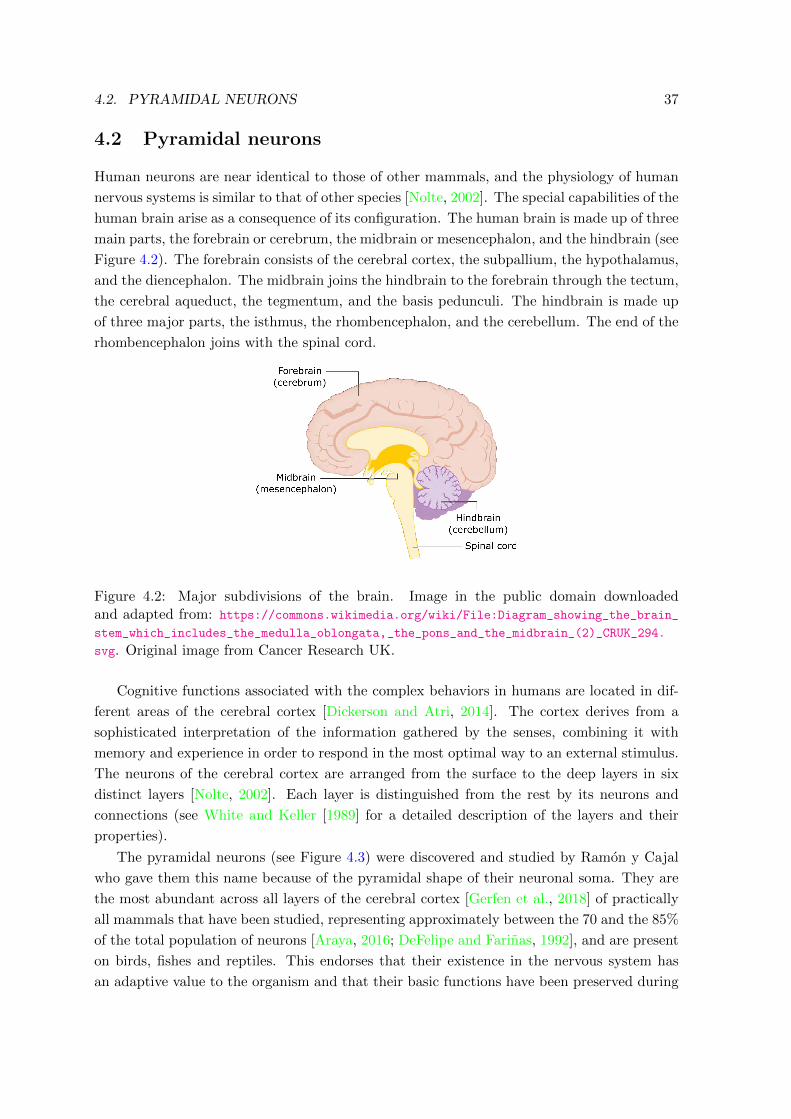
4.2. PYRAMIDAL NEURONS 37
4.2 Pyramidal neurons
Human neurons are near identical to those of other mammals, and the physiology of human
nervous systems is similar to that of other species [Nolte, 2002]. The special capabilities of the
human brain arise as a consequence of its configuration. The human brain is made up of three
main parts, the forebrain or cerebrum, the midbrain or mesencephalon, and the hindbrain (see
Figure 4.2). The forebrain consists of the cerebral cortex, the subpallium, the hypothalamus,
and the diencephalon. The midbrain joins the hindbrain to the forebrain through the tectum,
the cerebral aqueduct, the tegmentum, and the basis pedunculi. The hindbrain is made up
of three major parts, the isthmus, the rhombencephalon, and the cerebellum. The end of the
rhombencephalon joins with the spinal cord.
Figure 4.2: Major subdivisions of the brain. Image in the public domain downloadedand adapted from: https://commons.wikimedia.org/wiki/File:Diagram_showing_the_brain_
stem_which_includes_the_medulla_oblongata,_the_pons_and_the_midbrain_(2)_CRUK_294.
svg. Original image from Cancer Research UK.
Cognitive functions associated with the complex behaviors in humans are located in dif-
ferent areas of the cerebral cortex [Dickerson and Atri, 2014]. The cortex derives from a
sophisticated interpretation of the information gathered by the senses, combining it with
memory and experience in order to respond in the most optimal way to an external stimulus.
The neurons of the cerebral cortex are arranged from the surface to the deep layers in six
distinct layers [Nolte, 2002]. Each layer is distinguished from the rest by its neurons and
connections (see White and Keller [1989] for a detailed description of the layers and their
properties).
The pyramidal neurons (see Figure 4.3) were discovered and studied by Ramon y Cajal
who gave them this name because of the pyramidal shape of their neuronal soma. They are
the most abundant across all layers of the cerebral cortex [Gerfen et al., 2018] of practically
all mammals that have been studied, representing approximately between the 70 and the 85%
of the total population of neurons [Araya, 2016; DeFelipe and Farinas, 1992], and are present
on birds, fishes and reptiles. This endorses that their existence in the nervous system has
an adaptive value to the organism and that their basic functions have been preserved during
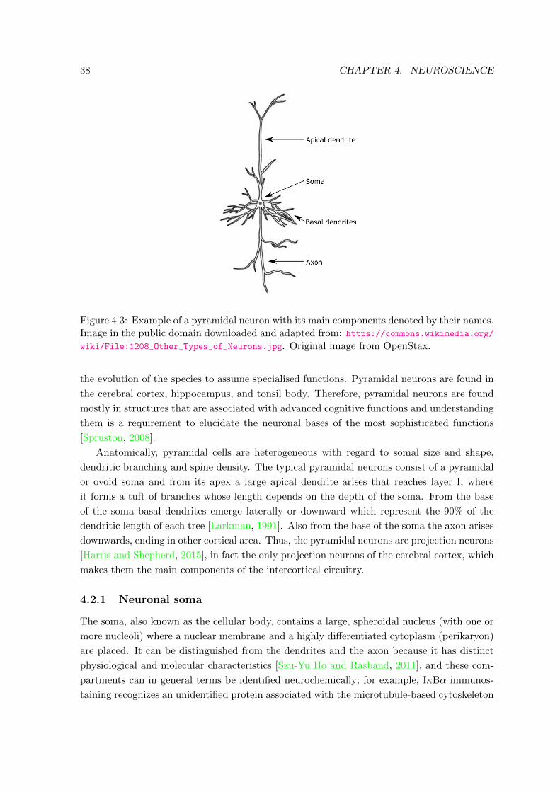
38 CHAPTER 4. NEUROSCIENCE
Figure 4.3: Example of a pyramidal neuron with its main components denoted by their names.Image in the public domain downloaded and adapted from: https://commons.wikimedia.org/
wiki/File:1208_Other_Types_of_Neurons.jpg. Original image from OpenStax.
the evolution of the species to assume specialised functions. Pyramidal neurons are found in
the cerebral cortex, hippocampus, and tonsil body. Therefore, pyramidal neurons are found
mostly in structures that are associated with advanced cognitive functions and understanding
them is a requirement to elucidate the neuronal bases of the most sophisticated functions
[Spruston, 2008].
Anatomically, pyramidal cells are heterogeneous with regard to somal size and shape,
dendritic branching and spine density. The typical pyramidal neurons consist of a pyramidal
or ovoid soma and from its apex a large apical dendrite arises that reaches layer I, where
it forms a tuft of branches whose length depends on the depth of the soma. From the base
of the soma basal dendrites emerge laterally or downward which represent the 90% of the
dendritic length of each tree [Larkman, 1991]. Also from the base of the soma the axon arises
downwards, ending in other cortical area. Thus, the pyramidal neurons are projection neurons
[Harris and Shepherd, 2015], in fact the only projection neurons of the cerebral cortex, which
makes them the main components of the intercortical circuitry.
4.2.1 Neuronal soma
The soma, also known as the cellular body, contains a large, spheroidal nucleus (with one or
more nucleoli) where a nuclear membrane and a highly differentiated cytoplasm (perikaryon)
are placed. It can be distinguished from the dendrites and the axon because it has distinct
physiological and molecular characteristics [Szu-Yu Ho and Rasband, 2011], and these com-
partments can in general terms be identified neurochemically; for example, IκBα immunos-
taining recognizes an unidentified protein associated with the microtubule-based cytoskeleton

4.2. PYRAMIDAL NEURONS 39
at the axon initial segment [Buffington et al., 2012] which can be used to demarcate the axon
initial segment [e.g., Sanchez-Ponce et al., 2012; Schultz et al., 2006]. Since the soma is the
cellular body, it contains the typical organelles of living cells (mitochondria, Golgi appara-
tus, ribosomes, lysosomes, etc.) that perform most of the metabolic activities in the neuron.
These components also support the chemical processing of the neuron that origins the neu-
rotransmitters, which are the basic elements of the synapses and consequently of the brain
activity. Soma also produces proteins for dendrites, axons and synaptic terminals.
The size of a neuronal soma can range from 0.005 mm to 0.1 mm in mammals. Its aspect
is highly variable taking diverse forms, being the most representatives the star, the fusiform,
the conical, the polyhedral, the spherical and the pyramidal. Specifically, the pyramidal
is usually represented as a tetrahedron with the acute angle pointing towards the surface
of the cortex. The morphology of the soma has been identified as one of the fundamental
features for discriminating between different types of neurons [Svoboda, 2011] and a statistical
relationship has been identified between the sizes of the soma and the neuron [Rajkovic et al.,
2016].
4.2.2 Dendrites
Dendrites are extensions of the neuron’s cellular body. Their main function is to receive
and process input synaptic signals. Dendrites show great structural diversity even within
one neuronal class [Ramaswamy et al., 2012] and knowing the shape of the dendritic tree it
is possible to indicate the type of connectivity that exists between certain neurons. Thus,
studying dendritic trees reveals mechanisms of function in a neuron in terms of its connectivity
and computation [Cuntz et al., 2014]. Differences in their morphologies are believed to be
related to functional differences [Krichmar et al., 2002; Vetter et al., 2001] and it is considered
that they play an important role in certain pathologies. For example, large and complex
dendrites in human pyramidal neurons have been associated with high IQ [Goriounova et al.,
2018]. Also neurodegenerative diseases, autism, Parkinson, Alzheimer and others have been
linked to changes in dendritic and axonal morphology [Kaufmann and Moser, 2000; Moolman
et al., 2004; Srivastava et al., 2012].
As mentioned above, the dendritic tree of a pyramidal neuron is divided into two types, the
basal dendrite that emerges from the base of the soma emanating a spherical arborization
and the apical dendrite that makes it from the apex of the soma. All pyramidal neurons
have several basal dendrites that are usually relatively short. Usually, a long apical dendrite
connects the soma to a bunch of dendrites. The characteristics of the dendrites of a pyramidal
neuron can vary considerably between different layers, cortical regions and species.
4.2.3 Dendritic spines
Dendrites are covered with thousands of dendritic spines (for simplicity’s sake, spines), that is,
small membranous protuberances each of which receives an excitatory synapse [Nimchinsky
et al., 2002]. Although their size and shape are quite heterogeneous, they all consist of a
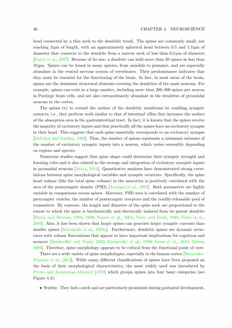
40 CHAPTER 4. NEUROSCIENCE
head connected by a thin neck to the dendritic trunk. The spines are commonly small, not
reaching 3 µm of length, with an approximately spherical head between 0.5 and 1.5 µm of
diameter that connects to the dendrite from a narrow neck of less than 0.5 µm of diameter
[Smith et al., 2007]. Because of its size, a dendrite can hold more than 50 spines in less than
10 µm. Spines can be found in many species, from annelids to primates, and are especially
abundant in the central nervous system of vertebrates. Their predominance indicates that
they must be essential for the functioning of the brain. In fact, in most areas of the brain,
spines are the dominant structural elements covering the dendrites of the main neurons. For
example, spines can exist in a large number, including more than 200, 000 spines per neuron
in Purkinje brain cells, and are also extraordinarily abundant in the dendrites of pyramidal
neurons in the cortex.
The spines try to extend the surface of the dendritic membrane by enabling synaptic
contacts, i.e., they perform work similar to that of intestinal villus that increases the surface
of the absorption area in the gastrointestinal tract. In fact, it is known that the spines receive
the majority of excitatory inputs and that practically all the spines have an excitatory synapse
in their head. This suggests that each spine essentially corresponds to an excitatory synapse
[DeFelipe and Farinas, 1992]. Thus, the number of spines represents a minimum estimate of
the number of excitatory synaptic inputs into a neuron, which varies ostensibly depending
on regions and species.
Numerous studies suggest that spine shape could determine their synaptic strength and
learning rules and is also related to the storage and integration of excitatory synaptic inputs
in pyramidal neurons [Araya, 2014]. Quantitative analyses have demonstrated strong corre-
lations between spine morphological variables and synaptic structure. Specifically, the spine
head volume (like the total spine volume) in the neocortex is positively correlated with the
area of the postsynaptic density (PSD) [Arellano et al., 2007]. Both parameters are highly
variable in comparisons across spines. Moreover, PSD area is correlated with the number of
presynaptic vesicles, the number of postsynaptic receptors and the readily-releasable pool of
transmitter. By contrast, the length and diameter of the spine neck are proportional to the
extent to which the spine is biochemically and electrically isolated from its parent dendrite
[Harris and Stevens, 1988, 1989; Nusser et al., 2001; Yuste and Denk, 1995; Yuste et al.,
2000]. Also, it has been shown that larger spines can generate larger synaptic currents than
smaller spines [Matsuzaki et al., 2004a]. Furthermore, dendritic spines are dynamic struc-
tures with volume fluctuations that appear to have important implications for cognition and
memory [Bonhoeffer and Yuste, 2002; Dunaevsky et al., 1999; Kasai et al., 2010; Matus,
2000]. Therefore, spine morphology appears to be critical from the functional point of view.
There are a wide variety of spine morphologies, especially in the human cortex [Benavides-
Piccione et al., 2013]. While many different classifications of spines have been proposed on
the basis of their morphological characteristics, the most widely used was introduced by
Peters and Kaiserman-Abramof [1970] which groups spines into four basic categories (see
Figure 4.4):
� Stubby: They lack a neck and are particularly prominent during postnatal development,

4.2. PYRAMIDAL NEURONS 41
Figure 4.4: Traditional classification of spines proposed in Peters and Kaiserman-Abramof[1970], adapted from Spruston [2008].
although they are also found among adults.
� Thin: The most common spines. They are composed by a thin and elongated neck and
a small bulbous head.
� Mushroom: Those that present a big head. Commonly they are found on adults.
� Filopodium: They are elongated and usually do not have a clearly distinguishable head.
However, it has also been argued that the large diversity of spine sizes reflects a continuum of
morphologies rather than the existence of discrete groups [Arellano et al., 2007]. Automatic
clustering techniques over 2D spine representations have recently been used [Bokota et al.,
2016; Ghani et al., 2016] to address this argument with the aim of avoiding the subjectivity
and bias involved in manual analyses. Both studies consider that some spines cannot be
clearly assigned to one of Peters and Kaiserman-Abramof’s classes because these spines are
transitions between shapes.
The literature about spines has related their morphology with some brain functionalities.
For example, it has been claimed that thin spines contribute to learning, while the biggest
and steady spines are linked to memory processes. Another objective they are believed to
accomplish is to increase the surface area of the dendritic area in order to group a large
number of synapses. They also play a role in regulating the electrical properties of the
neuron.
In view of the role played by spines in synaptic transmission, it is not surprising that a
large number of human mental illnesses are associated with alterations in their morphology
or density [Basu et al., 2018; Jacobs et al., 1997]. Some of these disorders are schizophrenia,
in which the density of spines in neocortical pyramidal neurons is below average; another is
aging, whose study has focused mainly on neocortical pyramidal neurons and in which it has
been observed that subjects over 50 showed a decrease of between 9% and 10% in the total
length of their dendrites and a reduction of nearly 50% in the number of spines compared to
individuals under 50 years old. Also in mental retardation, which shows a lower density of
spines in the neocortex and hippocampus and in abnormally short and long spines. These are
42 CHAPTER 4. NEUROSCIENCE
some examples to illustrate the importance of these components in brain functioning since
the list of disorders associated with spines is long and growing.
4.3 Computational neuroanatomy
Computational neuroscience [Churchland and Sejnowski, 1992; Dayan and Abbott, 2001]
emerges as a consequence of the incredible complexity of the brain to construct compact
representations of neurobiological processes through computer-assisted models and simulate
the structure of the nervous system to different scales. This research field provides the tools
to address the question of how nervous systems operate on the basis of known anatomy,
physiology and circuitry [Dayan and Abbott, 2001] by developing and testing hypotheses
of the functional mechanisms of the brain. Some brain models covered by computational
neuroscience are neuron and spike production [Dayan and Abbott, 2001; Eyal et al., 2018],
conductance-based models [Prinz et al., 2003], firing-rate models of large-scale circuit oper-
ation [Abbott, 1991; Heiberg et al., 2018], and computational generation and quantitative
morphometric analysis of virtual neurons [Ascoli et al., 2001].
Computational neuroanatomy [Ascoli, 1999, 2002] consists of the study of the shape and
structure of the nervous system. Data acquisition for the morphological analysis of a neuron
usually requires of cell-labeling methods such as those based on biocytin or green fluorescent
protein [Ascoli, 2006]. Then, a reconstruction of the neuron can be achieved using high-
throughput electron microscopy and software tools for 3D neuron tracing as for example
Neurolucida [Glaser and Glaser, 1990], FilamentTracer of Bitplane Imaris software [Worbs
and Forster, 2007] or Neuronstudio [Rodriguez et al., 2008; Wearne et al., 2005] among
others. These tools usually try to prevent or repair some artifacts introduced by noise, low
resolution introduced by the diffraction limitation, or background gradients [Meijering, 2010].
A reconstruction represents all the morphological information allowing for easy computation
and statistical analysis of a plethora of morphometric variables [Ascoli, 2006].
There are several options to quantify the neuronal structure [Meijering, 2010]. A distinc-
tion can be made between topological measures that focus exclusively on the connectivity
pattern and the analysis of physical distances, or between mathematical concepts such as
differential geometry, symmetry axes, and complexity [Costa et al., 2002]. Also different
approaches are followed depending on the neuronal component to be quantified. Soma is
usually evaluated in terms of its size and volume [Uylings and van Pelt, 2002], although
other geometrical measures as its sphericity or ellongation have been considered [Masseroli
et al., 1993]. Some basic morphometrics applied for the characterisation of dendrites are
total height, width, depth, length, volume of the tree and subtrees or the distance to the
soma [Lopez-Cruz et al., 2011]. Also a widely applied method is the Sholl analysis [Sholl,
1953] which uses concentric spheres to measure the spatial distribution of a dendritic arbor.
Dendritic spines are usually characterised by the head to neck ratio, head and neck diameter,
spine length and volume [Rodriguez et al., 2008; Shi et al., 2014]. Very recently, Basu et al.
[2018] have proposed a basic mathematical notation to define different key spine compart-
4.3. COMPUTATIONAL NEUROANATOMY 43
ments (e.g., spine head and spine neck) and have extracted some morphometric features as
the base of the spine, the central base point, the center of the head, and the tip of the spine
to classify the spines in the groups defined by Peters and Kaiserman-Abramof (see Figure
4.4).
4.3.1 Simulation of neuronal components
As discussed in Section 4.1, one of the main objectives of projects such as the Human Brain
Project, the Cajal Blue Brain or the BRAIN initiative is to create a large-scale simulation of
the brain using supercomputers. Computational neuroanatomy provides the tools to build
data-driven models from which to simulate virtual neuronal components. The parameters of
these models are computed from a set of random variables describing the morphology of the
neuronal component which reduces the problem of simulating to sampling from a probability
distribution. Advantages of this approach are that it is not necessary to store large volumes of
data because all the information is summarised in the mathematical model and moreover the
analysis of the model provides insights about the characteristics of the neuronal components.
Literature has mainly focused on the simulation of dendrite arborizations [Mainen and
Sejnowski, 1996; Vetter et al., 2001]. Usually, these algorithms perform a recursive branching
process where the characteristics of the following branches of the dendrite are sampled from
the model. Based on the software L-Neuron [Ascoli and Krichmar, 2000; Donohue et al.,
2002], Donohue and Ascoli [2008] examined dendritic elongation, branching, and taper to
stochastically generate bifurcations and branches. Lopez-Cruz et al. [2011] extended this
work including a more complete set of variables and using a BN to consider the relations
among the variables. Other software is NETMORPH [Koene et al., 2009], that simulates
neuronal morphogenesis from the perspective of an individual growth cone, stochastically
sampling the elongation, branching and turning of the dendritic tree.
Computational neuroscience has been also applied to recover or repair incomplete recon-
structions of cells. For example, dendritic arborisations can be incomplete when they pass
the limit of the microscope during the reconstruction process. A repairing algorithm was
presented in Anwar et al. [2009] based on a probabilistic analysis of branch characteristics
at various distances from the neuron soma. The method reconstructs the missing portion
of the incomplete dendritic arborisations by sampling branches from a pool of completely
reconstructed dendrites and joining them to the incomplete dendrites according to the simi-
larity between the completely reconstructed arborisations and the incomplete dendrites. Note
that this strategy makes strong assumptions about the morphology of the dendrites: (i) the
growth of the new dendritic branches only depends on the dendritic branches closer to the
soma and (ii) the pool of completely reconstructed dendrites is big enough to capture all
the fundamental dendritic morphologies. Also, soma is usually ignored or in the best case
assumed to be a sphere by neuron tracing software. Neuronize [Brito et al., 2013] consists of
a set of methods designed to build a realistic and accurate 3D shape of the soma from the
incomplete information stored in the digitally traced neuron.

44 CHAPTER 4. NEUROSCIENCE
4.3.2 Bayesian networks in neuroanatomy
BNs are a suitable tool for modelling in neuroscience given that they provide the mech-
anisms to learn the relations between variables and perform probabilistic reasoning un-
der uncertainty. They have been succesfully applied in several neuroscientific problems as
neuroanatomy, electrophysiology, genomics, proteomics, transcriptomics, and neuroimaging
[Bielza and Larranaga, 2014].
One of the problems addressed through BNs in neuroanatomy is the classification of
GABAergic interneurons according to axonal arborization patterns [DeFelipe et al., 2013].
Lopez-Cruz et al. [2014] developed a web-based interactive system where 42 experts in the
field described the axonal arborization of 320 cortical interneurons according to six variables.
Then, they developed a consensus model in the form of a Bayesian multinet learning a BN
classifier from the data of each expert to discriminate among the interneuron classes. Based
on the same dataset, Mihaljevic et al. [2015] form different subsets of neurons by increasing
the threshold on label reliability, which they defined as the minimal number of neuroscientist
agreeing on the majority type of neuron. Then, they apply BN classifiers on each data subset
to test if reliability on the type of neuron can help to categorized interneurons accurately.
Also Mihaljevic et al. [2018] trained several classification algorithms to classify a set of 217
rat interneurons.
Bayesian classifiers have been also applied to discriminate between pyramidal cells and
interneurons from mouse neocortex based on their morphological features. Guerra et al. [2011]
used a database of 327 cells and 65 morphological features for learning a naıve Bayes classifer,
among other models, and evaluated the performance against a test dataset to automatically
distinguish between pyramidal cells and interneurons (without using the existence/absence
of the apical dendrite as a predictor feature).
As discussed above, BNs have been used to model and simulate dendritic trees. Lopez-
Cruz et al. [2011] measured a set of morphological variables from layer III pyramidal neurons
from different regions of the mouse neocortex collection information mainly about the sub-
tree and subdendrite, segment length, orientation, and bifurcation. Then, they suggested a
simulation algorithm to generate virtual dendrites by sampling from the BNs.
Part III
CONTRIBUTIONS TO
DIRECTIONAL STATISTICS
AND DATA CLUSTERING
45

Chapter 5Directional-linear Bayesian
networks for clustering
5.1 Introduction
The study of a plethora of phenomena requires the measurement of their magnitude and
direction. Examples are meteorology [Carta et al., 2008], rhythmometry, medicine, demog-
raphy [Batschelet et al., 1973; Batschelet, 1981], earthquake prediction [Love and Thomas,
2013; Thomas et al., 2009a,b, 2012] or neuroscience [Leguey, 2018]. Typically, when this
data is collected, an exploratory analysis is performed to reveal patterns. Cluster analysis
partitions data into groups of homogeneous observations. A probabilistic clustering approach
is model-based clustering [Fraley and Raftery, 2002; McLachlan and Basford, 1988; Melnykov
and Maitra, 2010]. Finite mixtures of Gaussians are the most commonly used distribution
in model-based clustering because they can approximate any non-directional multivariate
density given enough components [Titterington et al., 1985]. However, directional data has
special properties that conventional statistics cannot handle. To address this problem several
distributions have been proposed in the directional statistics literature to cluster directional-
linear data (see Section 3.3.3 and Section 3.4). The main drawbacks of these models are that
it is complex to extend them beyond the bivariate case and they have restrictive assumptions
of conditional independence among the variables that limits their expressiveness.
Here we propose approaches based on exploiting the conditional independence assump-
tions encoded by a BN to enable efficient clustering of multivariate directional-linear data.
We introduce three mixture models, from simpler to more expressive. We start defining a
naıve Bayes mixture model to cluster multivariate directional data to finally introduce the
Extended Mardia-Sutton mixture model, whose mixture components are distributed accord-
ing to a newly proposed multivariate probability density function represented as a BN that
is able to capture the directional-linear correlations. Thus, the latter mixture model extends
the previous models proposed in the literature by relaxing the independence constraints to
include relations between directional and linear variables. Additionally, we use the SEM al-
47
48 CHAPTER 5. DIRECTIONAL-LINEAR
gorithm [Friedman, 1997] to capture the relations among the random variables at the same
time that we discover the clusters. We also derive the Kullback-Leibler divergence [Kullback
and Leibler, 1951] and Bhattacharyya distance [Bhattacharyya, 1946] for these models as
measures of the quality of the clustering outcomes.
Experimental results will empirically demonstrate the advantages of performing cluster-
ing using directional-linear clustering techniques over using Gaussian mixture models which
cannot capture the periodicity of directional data leading to poor approximations. Numerical
evaluation of our clustering methods suggest that the learned models always obtain better
results than a Gaussian mixture model in the presence of directional data and that they
are able to discover the conditional independence relationships between variables during the
clustering process.
The content of this chapter has been published in Luengo-Sanchez et al. [2016] and
Luengo-Sanchez et al. [2019].
Chapter outline
In Section 5.2 we propose a finite mixture model based on the naıve Bayes assumption to
obtain closed-form equations for clustering multivariate directional data. In Section 5.3 we
add linear variables to the above model, learning the conditional dependences between the
linear variables through the SEM algorithm. In Section 5.4 we propose a generalisation
of the previous models based on the new Extended Mardia-Sutton distribution to include
directional-linear relations between variables. For the models proposed in Section 5.2, Section
5.3 and Section 5.4 we derive the Kullback-Leibler divergence and the Bhattacharyya distance
as measures of similarity between the mixture components. We provide experimental results
that numerically evaluate the suitability of the models. Section 5.5 closes the chapter with
the conclusions.
5.2 Naıve Bayes von Mises mixture model
Here, we exploit the conditional independence encoded by BNs to perform efficient clustering
of directional data D = {y1, ...,yN} distributed according to the vector of directional random
variables Y. Our assumptions about the model are that the dataset D has no missing values,
that the directional variables in set Y are conditionally independent given the latent variable
Z and that the directional variables follow the vM distribution. Figure 5.1 shows a graphical
representation of the BN structure for the proposed model which corresponds to the NB
model.
We choose the NB structure because its factorisation can solve the problems related to
parameter estimation for the multivariate vM distribution. To exploit the benefits of NB
factorisation, however, data must be complete. This is not the case in clustering because
latent variable Z is unobserved. Hence, we need to apply the EM algorithm. First, we
compute the expected values of Z for the cluster 1, ...,K, where K is the number of clusters,
according to the E-step (Equation (2.12)). This completes the data so, according to Equation
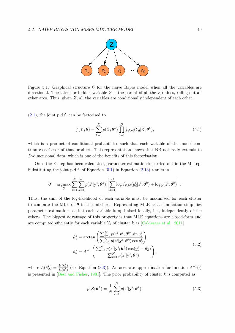
5.2. NAIVE BAYES VON MISES MIXTURE MODEL 49
Figure 5.1: Graphical structure G for the naıve Bayes model when all the variables aredirectional. The latent or hidden variable Z is the parent of all the variables, ruling out allother arcs. Thus, given Z, all the variables are conditionally independent of each other.
(2.1), the joint p.d.f. can be factorised to
f(Y;θ) =
K∑k=1
p(Z;θk)
D∏d=1
fVM(Yd|Z;θk), (5.1)
which is a product of conditional probabilities such that each variable of the model con-
tributes a factor of that product. This representation shows that NB naturally extends to
D-dimensional data, which is one of the benefits of this factorisation.
Once the E-step has been calculated, parameter estimation is carried out in the M-step.
Substituting the joint p.d.f. of Equation (5.1) in Equation (2.13) results in
θ = argmaxθ
N∑i=1
K∑k=1
p(zi|yi;θk)
[D∑d=1
log fVM(yid|zi;θk) + log p(zi;θk)
].
Thus, the sum of the log-likelihood of each variable must be maximised for each cluster
to compute the MLE of θ in the mixture. Representing MLE as a summation simplifies
parameter estimation so that each variable is optimised locally, i.e., independently of the
others. The biggest advantage of this property is that MLE equations are closed-form and
are computed efficiently for each variable Yd of cluster k as [Calderara et al., 2011]
µkd = arctan
(∑Ni=1 p(z
i|yi;θk) sin yid∑Ni=1 p(z
i|yi;θk) cos yid
),
κkd = A−1
(∑Ni=1 p(z
i|yi;θk) cos(yid − µkd)∑Ni=1 p(z
i|yi;θk)
),
(5.2)
where A(κkd) =I1(κkd)
I0(κkd)(see Equation (3.3)). An accurate approximation for function A−1(·)
is presented in [Best and Fisher, 1981]. The prior probability of cluster k is computed as
p(Z;θk) =1
N
N∑i=1
p(zi|yi;θk). (5.3)
50 CHAPTER 5. DIRECTIONAL-LINEAR
This approach based on exploiting independence constraints avoids the numerical optimi-
sation needed for the mixtures of bivariate and multivariate vM distributions [Mardia et al.,
2007, 2012]. It also ensures that the likelihood increases monotonically in each step of the
EM algorithm until convergence to a local maximum even though data is not highly concen-
trated. The main limitation of this model is that it assumes conditional independence among
all the variables within each cluster. Although there are few real-world cases where the NB
assumption holds, usually its accuracy is competitive and it has a small generalisation error.
5.2.1 Kullback-Leibler divergence and Bhattacharyya distance
The performance of the clustering algorithms depends on the separability of the mixture com-
ponents [Sun and Wang, 2011]. In addition, the identification and interpretation of clusters
are easier when groups are homogeneous, i.e., when the instances ascribed to each cluster
belong to their cluster with a high probability. The overlap between probability distributions
provides a quantitative description of these desirable properties, but its computation is often
intractable analytically. For this reason, overlapping is usually replaced by similarity mea-
sures between distributions. Among them, the most widely used are the relative entropy or
Kullback-Leibler divergence (KL) and the Bhattacharyya distance (BD) . The KL divergence
and the BD can be expressed in closed-form for the above model after decomposing the joint
p.d.f. according to the independence assumptions encoded by the BN structure.
5.2.1.1 Kullback-Leibler divergence
The KL divergence is defined as a measure of the difference between two distributions
DKL(P (Y)||Q(Y)) =
∫YP (Y) log
P (Y)
Q(Y)dY,
where P (Y) and Q(Y) denote, respectively, the p.d.f. of distributions P and Q for a set of
random variables. In this case, the KL divergence factorises according to the chain rule of
relative entropy [Cover and Thomas, 1991] as
DKL(P (Y)||Q(Y)) =
D∑d=1
DKL(P (Yd)||Q(Yd)).
Thus, the KL divergence for the joint p.d.f. decomposes as a sum of KL divergences between
univariate vM distributions.
We define the two univariate vM distributions P (Yd) and Q(Yd) (Equation (3.2)) for the
directional variable Yd as
P (Yd) = fVM(Yd;µPd , κ
Pd ) and Q(Yd) = fVM(Yd;µ
Qd , κ
Qd )
respectively. Then, for the sake of simplicity in the calculations, distributions P (Yd) and
Q(Yd) are rotated according to µPd , giving as results the means µpd = µPd − µPd = 0 and

5.2. NAIVE BAYES VON MISES MIXTURE MODEL 51
µqd = µQd − µPd . The concentration parameters of the rotated distributions does not change
after the transformation operation so κpd = κPd and κqd = κQd . Note that the rotation does
not change the concentration of the distributions. The KL divergence for the univariate vM
distribution after the rotation is
DKL(P (Yd)||Q(Yd)) = log I0(κqd)− log I0(κpd) +A(κpd)(κpd − κ
qd cos(µqd)
). (5.4)
A detailed derivation of this KL divergence between two univariate vM distributions can be
found in Appendix B.3.
5.2.1.2 Bhattacharyya distance
The BD is a measure of the separability between two distributions that has been widely used
in classification [Fukunaga, 1972]
DB(P (Y), Q(Y)) = − ln
(∫Y
√P (Y), Q(Y)
)dY.
The computation of the BD also benefits from the conditional NB assumption. More con-
cretely, the BD factorises according to
BD(P (Y), Q(Y)) = − ln
∫Y
√√√√ D∏d=1
fVM(Yd;µPd , κ
Pd ) ·
D∏d=1
fVM(Yd;µQd , κ
Qd )dY
= − ln
D∏d=1
1
2π√I0(κPd )I0(κQd )
∫YeκPd2
cos(Yd−µPd )eκQd2
cos(Yd−µQd )dY
= − lnD∏d=1
BC(P (Yd), Q(Yd)) =D∑d=1
BD(P (Yd), Q(Yd)),
(5.5)
giving as result a closed-form expression that consists of the sum of univariate BD. The BD
between two univariate vM distributions is derived in Appendix B.2 as
BD(P (Yd), Q(Yd)) = − lnBC(P (Yd), Q(Yd)) = − ln(I0(R)) +ln(I0(κPd )) + ln(I0(κPd ))
2,
where
R =√a2 + b2
a =κPd2
cos(µPd ) +κQd2
cos(µQd )
b =κPd2
sin(µPd ) +κQd2
sin(µQd ).
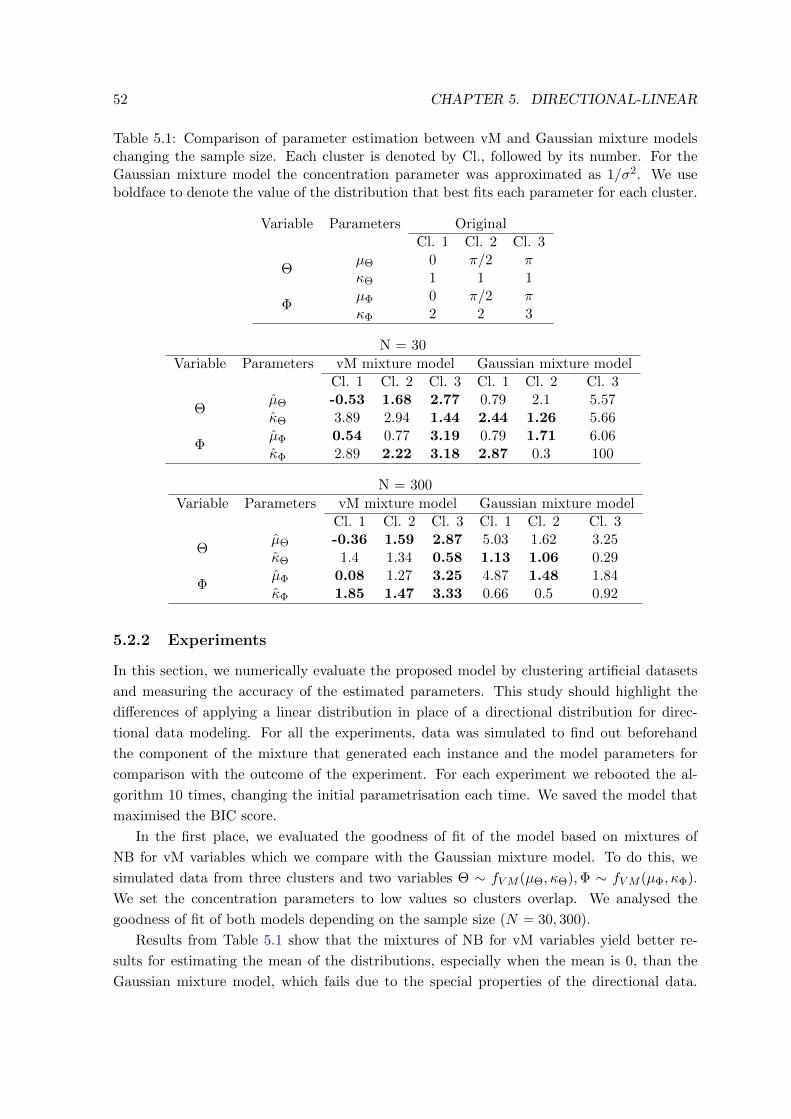
52 CHAPTER 5. DIRECTIONAL-LINEAR
Table 5.1: Comparison of parameter estimation between vM and Gaussian mixture modelschanging the sample size. Each cluster is denoted by Cl., followed by its number. For theGaussian mixture model the concentration parameter was approximated as 1/σ2. We useboldface to denote the value of the distribution that best fits each parameter for each cluster.
Variable Parameters OriginalCl. 1 Cl. 2 Cl. 3
ΘµΘ 0 π/2 πκΘ 1 1 1
ΦµΦ 0 π/2 πκΦ 2 2 3
N = 30
Variable Parameters vM mixture model Gaussian mixture modelCl. 1 Cl. 2 Cl. 3 Cl. 1 Cl. 2 Cl. 3
ΘµΘ -0.53 1.68 2.77 0.79 2.1 5.57κΘ 3.89 2.94 1.44 2.44 1.26 5.66
ΦµΦ 0.54 0.77 3.19 0.79 1.71 6.06κΦ 2.89 2.22 3.18 2.87 0.3 100
N = 300
Variable Parameters vM mixture model Gaussian mixture modelCl. 1 Cl. 2 Cl. 3 Cl. 1 Cl. 2 Cl. 3
ΘµΘ -0.36 1.59 2.87 5.03 1.62 3.25κΘ 1.4 1.34 0.58 1.13 1.06 0.29
ΦµΦ 0.08 1.27 3.25 4.87 1.48 1.84κΦ 1.85 1.47 3.33 0.66 0.5 0.92
5.2.2 Experiments
In this section, we numerically evaluate the proposed model by clustering artificial datasets
and measuring the accuracy of the estimated parameters. This study should highlight the
differences of applying a linear distribution in place of a directional distribution for direc-
tional data modeling. For all the experiments, data was simulated to find out beforehand
the component of the mixture that generated each instance and the model parameters for
comparison with the outcome of the experiment. For each experiment we rebooted the al-
gorithm 10 times, changing the initial parametrisation each time. We saved the model that
maximised the BIC score.
In the first place, we evaluated the goodness of fit of the model based on mixtures of
NB for vM variables which we compare with the Gaussian mixture model. To do this, we
simulated data from three clusters and two variables Θ ∼ fVM (µΘ, κΘ),Φ ∼ fVM (µΦ, κΦ).
We set the concentration parameters to low values so clusters overlap. We analysed the
goodness of fit of both models depending on the sample size (N = 30, 300).
Results from Table 5.1 show that the mixtures of NB for vM variables yield better re-
sults for estimating the mean of the distributions, especially when the mean is 0, than the
Gaussian mixture model, which fails due to the special properties of the directional data.

5.3. HYBRID GAUSSIAN-VON MISES MIXTURE MODEL 53
Table 5.2: Hit rate of vM vs Gaussian mixture models. We simulated 100 instances fromeach cluster. The best results are denoted in boldface.
vM mixture model Gaussian mixture modelN. Cl./N. Var. 10 25 50 10 25 50
3 99% 100% 100% 94.6% 99.6% 68.33%5 97% 100% 100% 47.2% 59.2% 100%10 56.2% 99.1% 100% 38.7% 40.4% 38.3%
When the sample size increases, the proposed model further improves the estimation of the
concentration parameters.
Then, we evaluated the performance of the clustering algorithm by changing the number
of clusters (K = 3, 5, 10) and variables (M = 10, 25, 50). Modifying the number of variables
provides information about the accuracy of the model when data is concentrated or sparse.
Varying the number of clusters in a bounded and fixed space we measure the performance
of the method as more clusters overlap. For the experiment, complete data was available,
i.e., variables and cluster labels were known. We started by hiding the cluster label of all
instances and clustering the data. We crisply assigned each instance to the cluster with
maximum membership probability. As a result, each instance belonged to one group. Then,
we compared the real label with label provided by the clustering algorithm to get its hit rate.
The accuracy of the proposed model was compared against the Gaussian mixture model, see
Table 5.2.
Analysing Table 5.2 we find that mixtures of vM distributions improve their accuracy as
the number of variables increases. This is because clusters are further apart and consequently
easily separated in higher dimensions. The opposite applies when the number of clusters
grows. In this case the clusters overlap. Therefore, the boundaries between them are not
clearly defined, and clustering algorithms are less accurate. However, the Gaussian mixture
model behaves differently. Even though data sparsity increases when the number of variables
is 50, the accuracy of Gaussian variables decays for 3 and 10 clusters with respect to the case
when there are 25 variables. For all cases vM clustering achieves better results than Gaussian
mixture models.
5.3 Hybrid Gaussian-von Mises mixture model
As discussed in Section 3.1, some practical scenarios involve several linear and directional
variables. The clustering models proposed under this data configuration are generally based
on learning multivariate probability distributions whose variables are conditionally indepen-
dent given the latent variable (Section 3.4). The representation of these models as a BN is
equivalent to preset a fixed structure. However, discovering the graph topology provides in-
formation about the relations of dependence between variables and may improve the model’s
accuracy. The SEM algorithm (see Section 2.5 and Algorithm 1) defines a flexible approach to
clustering, automatically learning the structure of the network during the clustering process.
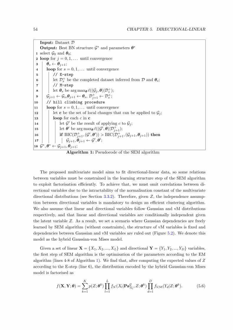
54 CHAPTER 5. DIRECTIONAL-LINEAR
Input: Dataset DOutput: Best BN structure G∗ and parameters θ∗
1 select G0 and θ0;2 loop for j = 0, 1, . . . until convergence3 θs ← θj+1;4 loop for s = 0, 1, . . . until convergence5 // E-step
6 let D+s be the completed dataset inferred from D and θs;
7 // M-step
8 let θs be arg maxθ `((Gj ,θ)|D+s );
9 Gj+1 ← Gs,θj+1 ← θs, D+j+1 ← D+
s ;
10 // hill climbing procedure
11 loop for s = 0, 1, . . . until convergence12 let c be the set of local changes that can be applied to Gj ;13 loop for each c in c14 let G′ be the result of applying c to Gj ;15 let θ′ be arg maxθ `((G′,θ)|D+
j+1);
16 if BIC(D+j+1, (G′,θ′)) > BIC(D+
j+1, (Gj+1,θj+1)) then
17 Gj+1,θj+1 ← G′,θ′;18 G∗,θ∗ ← Gj+1,θj+1;
Algorithm 1: Pseudocode of the SEM algorithm
The proposed multivariate model aims to fit directional-linear data, so some relations
between variables must be constrained in the learning structure step of the SEM algorithm
to exploit factorisation efficiently. To achieve that, we must omit correlations between di-
rectional variables due to the intractability of the normalisation constant of the multivariate
directional distributions (see Section 3.3.2). Therefore, given Z, the independence assump-
tion between directional variables is mandatory to design an efficient clustering algorithm.
We also assume that linear and directional variables follow Gaussian and vM distributions
respectively, and that linear and directional variables are conditionally independent given
the latent variable Z. As a result, we set a scenario where Gaussian dependencies are freely
learned by SEM algorithm (without constraints), the structure of vM variables is fixed and
dependencies between Gaussian and vM variables are ruled out (Figure 5.2). We denote this
model as the hybrid Gaussian-von Mises model.
Given a set of linear X = {X1, X2, ..., XL} and directional Y = {Y1, Y2, ..., YD} variables,
the first step of SEM algorithm is the optimisation of the parameters according to the EM
algorithm (lines 4-8 of Algorithm 1). We find that, after computing the expected values of Z
according to the E-step (line 6), the distribution encoded by the hybrid Gaussian-von Mises
model is factorised as
f(X,Y;θ) =
K∑k=1
p(Z;θk)
L∏l=1
fN (Xl|PaGXl , Z;θk)
D∏d=1
fVM(Yd|Z;θk). (5.6)

5.3. HYBRID GAUSSIAN-VON MISES MIXTURE MODEL 55
Figure 5.2: An example of the graphical structure G for the hybrid Gaussian-von Mises model.The structure of Gaussian variables is learnt during the clustering process. vM variables areindependent given Z which is the parent of all the variables. There is no dependence betweenGaussian and vM variables.
where PaGXl ⊂ {X, Z} and Z ∈ PaGXl . Here, the difference between Equations (5.1) and
(5.6) lies in the product of conditional Gaussian distributions. Given the set of parents
PaGXl = {U1l, ..., UT l, Z} of variable Xl in Equation (5.6), each linear Gaussian (see Section
2.4.3.2) is defined as
fN (Xl|PaGl ;θk) = fN (βk0l + βkl>
X, σ2,kl ) = fN (βk0l +
T∑t=1
βktlUtl, σ2,kl ),
where (βk0l,βkl ) is the vector of regression coefficients and σ2,k
l is the variance of variable Xl
for cluster k, βktl are the non-zero coefficients in βkl , and T are the number of βktl coefficients.
Note that, for those variables X 6∈ PaGXl , their regression coefficients are zero. When the only
parent of a Gaussian variable is Z, then β0k = µkl .
In Section 5.2, NB dependence constraints among variables were exploited to factorise
the joint p.d.f. as a product where each factor corresponded to one variable. When they
were combined using the EM algorithm to estimate the cluster parameters, the parameters of
each variable were maximised independently of the others, resulting in closed-form equations.
The advantages provided by the factorisation of the NB structure on directional data are now
extrapolated to achieve a model for multidimensional hybrid data. Parameter estimation is
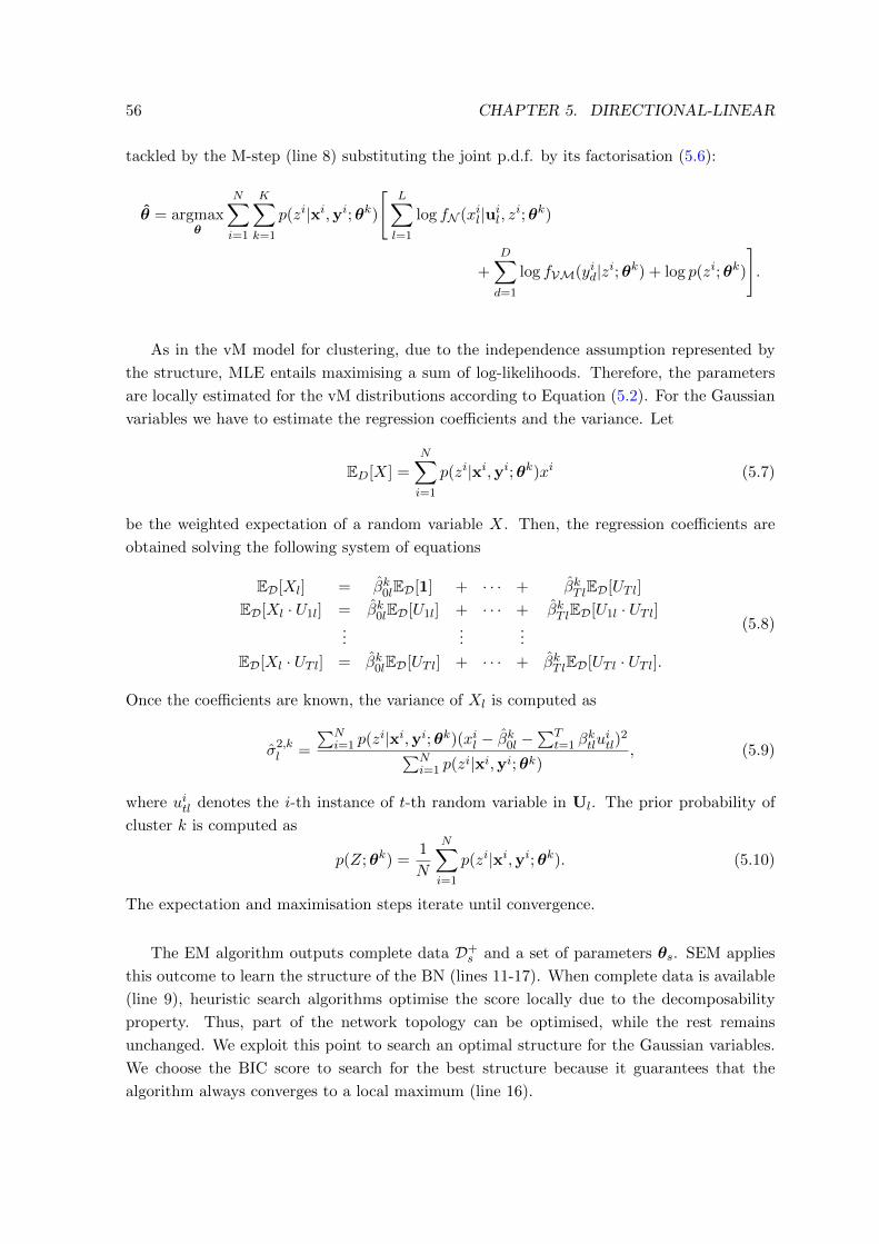
56 CHAPTER 5. DIRECTIONAL-LINEAR
tackled by the M-step (line 8) substituting the joint p.d.f. by its factorisation (5.6):
θ = argmaxθ
N∑i=1
K∑k=1
p(zi|xi,yi;θk)
[L∑l=1
log fN (xil|uil, zi;θk)
+
D∑d=1
log fVM(yid|zi;θk) + log p(zi;θk)
].
As in the vM model for clustering, due to the independence assumption represented by
the structure, MLE entails maximising a sum of log-likelihoods. Therefore, the parameters
are locally estimated for the vM distributions according to Equation (5.2). For the Gaussian
variables we have to estimate the regression coefficients and the variance. Let
ED[X] =
N∑i=1
p(zi|xi,yi;θk)xi (5.7)
be the weighted expectation of a random variable X. Then, the regression coefficients are
obtained solving the following system of equations
ED[Xl] = βk0lED[1] + · · · + βkT lED[UT l]
ED[Xl · U1l] = βk0lED[U1l] + · · · + βkT lED[U1l · UT l]...
......
ED[Xl · UT l] = βk0lED[UT l] + · · · + βkT lED[UT l · UT l].
(5.8)
Once the coefficients are known, the variance of Xl is computed as
σ2,kl =
∑Ni=1 p(z
i|xi,yi;θk)(xil − βk0l −∑T
t=1 βktlu
itl)
2∑Ni=1 p(z
i|xi,yi;θk), (5.9)
where uitl denotes the i-th instance of t-th random variable in Ul. The prior probability of
cluster k is computed as
p(Z;θk) =1
N
N∑i=1
p(zi|xi,yi;θk). (5.10)
The expectation and maximisation steps iterate until convergence.
The EM algorithm outputs complete data D+s and a set of parameters θs. SEM applies
this outcome to learn the structure of the BN (lines 11-17). When complete data is available
(line 9), heuristic search algorithms optimise the score locally due to the decomposability
property. Thus, part of the network topology can be optimised, while the rest remains
unchanged. We exploit this point to search an optimal structure for the Gaussian variables.
We choose the BIC score to search for the best structure because it guarantees that the
algorithm always converges to a local maximum (line 16).
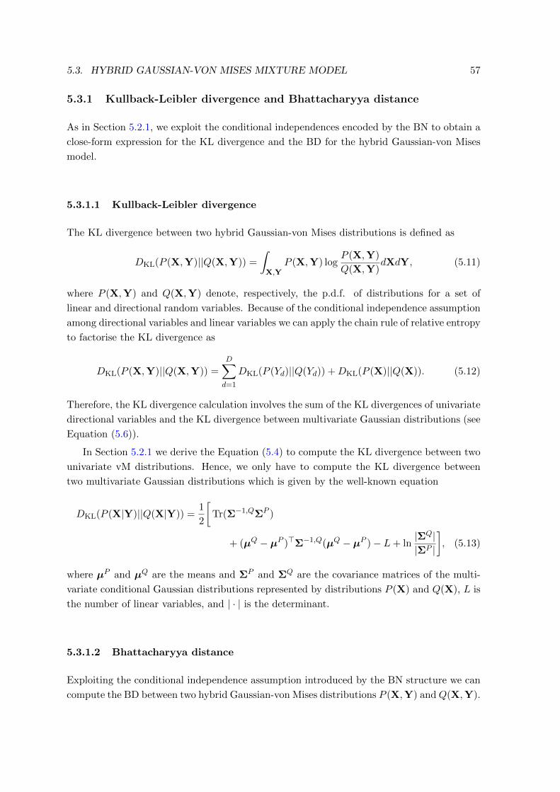
5.3. HYBRID GAUSSIAN-VON MISES MIXTURE MODEL 57
5.3.1 Kullback-Leibler divergence and Bhattacharyya distance
As in Section 5.2.1, we exploit the conditional independences encoded by the BN to obtain a
close-form expression for the KL divergence and the BD for the hybrid Gaussian-von Mises
model.
5.3.1.1 Kullback-Leibler divergence
The KL divergence between two hybrid Gaussian-von Mises distributions is defined as
DKL(P (X,Y)||Q(X,Y)) =
∫X,Y
P (X,Y) logP (X,Y)
Q(X,Y)dXdY, (5.11)
where P (X,Y) and Q(X,Y) denote, respectively, the p.d.f. of distributions for a set of
linear and directional random variables. Because of the conditional independence assumption
among directional variables and linear variables we can apply the chain rule of relative entropy
to factorise the KL divergence as
DKL(P (X,Y)||Q(X,Y)) =D∑d=1
DKL(P (Yd)||Q(Yd)) +DKL(P (X)||Q(X)). (5.12)
Therefore, the KL divergence calculation involves the sum of the KL divergences of univariate
directional variables and the KL divergence between multivariate Gaussian distributions (see
Equation (5.6)).
In Section 5.2.1 we derive the Equation (5.4) to compute the KL divergence between two
univariate vM distributions. Hence, we only have to compute the KL divergence between
two multivariate Gaussian distributions which is given by the well-known equation
DKL(P (X|Y)||Q(X|Y)) =1
2
[Tr(Σ−1,QΣP )
+ (µQ − µP )>Σ−1,Q(µQ − µP )− L+ ln|ΣQ||ΣP |
], (5.13)
where µP and µQ are the means and ΣP and ΣQ are the covariance matrices of the multi-
variate conditional Gaussian distributions represented by distributions P (X) and Q(X), L is
the number of linear variables, and | · | is the determinant.
5.3.1.2 Bhattacharyya distance
Exploiting the conditional independence assumption introduced by the BN structure we can
compute the BD between two hybrid Gaussian-von Mises distributions P (X,Y) andQ(X,Y).

58 CHAPTER 5. DIRECTIONAL-LINEAR
Because the linear variables are assumed to be Gaussian, the BD factorises as
BD(P (X,Y), Q(X,Y)) = − ln
∫X
∫Y
√√√√fN (X;µP ,ΣP )D∏d=1
fVM(Yd|µPd , κPd )
·
√√√√fN (X;µQ,ΣQ)
D∏d=1
fVM(Yd|µQd , κQd ).
Note that bold µ denotes the mean of the multivariate Gaussian while µd refers to the mean
of the directional variable d. Then, as the linear and directional variables are independent,
we can reorder the terms as
BD(P (X,Y), Q(X,Y)) =− ln
∫X
√fN (X;µP ,ΣP )fN (X;µQ,ΣQ)
− ln
∫Y
√fVM(Yd|µPd , κPd )fVM(Yd|µQd , κ
Qd ).
Therefore, the BD is computed locally for linear and directional variables. The the well-known
expression for the BD between two multivariate Gaussian is
BD(fN (X;µP ,ΣP ), fN (X;µQ,ΣQ)) =1
8(µP −µQ)>Σ−1(µP −µQ) +
1
2ln
(|Σ|√|ΣP ||ΣQ|
).
(5.14)
where Σ = ΣP+ΣQ
2 . In Section 5.2.1.2 we introduced the expression for the BD between
two multivariate vM distributions where all its variables are conditionally independent (see
Equation (5.5)). Hence, the BD between two hybrid Gaussian-von Mises distributions can
be computed as
BD(P (X,Y), Q(X,Y)) =1
8(µP − µQ)>Σ−1(µP − µQ) +
1
2ln
(|Σ|√|ΣP ||ΣQ|
)
−D∑d=1
ln(I0(R)) +ln(I0(κPd )) + ln(I0(κPd ))
2
5.3.2 Experiments
To achieve a deeper insight into the suitability of the hybrid Gaussian-von Mises model
for clustering tasks, we evaluate it numerically clustering artificial datasets and measuring
the accuracy of the estimated parameters. More concretely, we adapted the experiments of
Section 5.2.2 to directional-linear data. We started by validating the goodness of fit and the
structure learnt by the model. To do this, we manually defined a BN with five Gaussian
nodes and two vM nodes (Figure 5.3) setting the number of clusters to 3. We simulated 100
instances of this BN for each cluster. Then, we applied the hybrid Gaussian-von Mises model
to learn the model parameters and the structure from Gaussian variables.
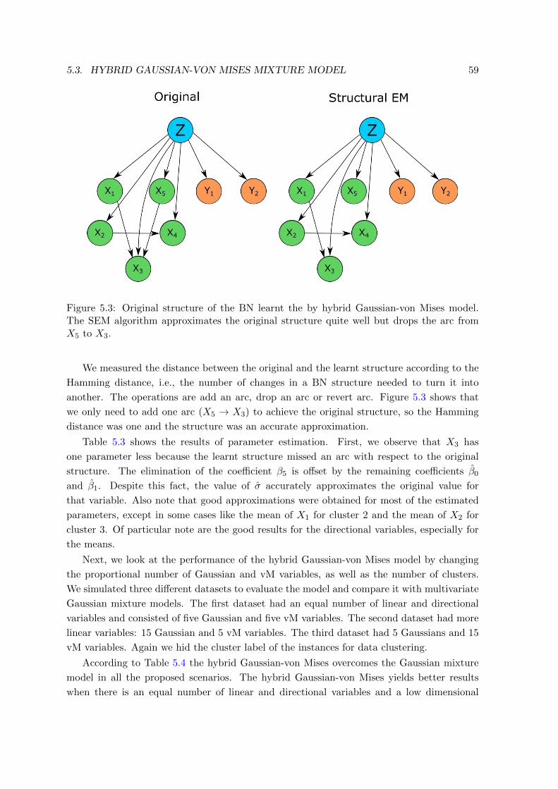
5.3. HYBRID GAUSSIAN-VON MISES MIXTURE MODEL 59
Figure 5.3: Original structure of the BN learnt the by hybrid Gaussian-von Mises model.The SEM algorithm approximates the original structure quite well but drops the arc fromX5 to X3.
We measured the distance between the original and the learnt structure according to the
Hamming distance, i.e., the number of changes in a BN structure needed to turn it into
another. The operations are add an arc, drop an arc or revert arc. Figure 5.3 shows that
we only need to add one arc (X5 → X3) to achieve the original structure, so the Hamming
distance was one and the structure was an accurate approximation.
Table 5.3 shows the results of parameter estimation. First, we observe that X3 has
one parameter less because the learnt structure missed an arc with respect to the original
structure. The elimination of the coefficient β5 is offset by the remaining coefficients β0
and β1. Despite this fact, the value of σ accurately approximates the original value for
that variable. Also note that good approximations were obtained for most of the estimated
parameters, except in some cases like the mean of X1 for cluster 2 and the mean of X2 for
cluster 3. Of particular note are the good results for the directional variables, especially for
the means.
Next, we look at the performance of the hybrid Gaussian-von Mises model by changing
the proportional number of Gaussian and vM variables, as well as the number of clusters.
We simulated three different datasets to evaluate the model and compare it with multivariate
Gaussian mixture models. The first dataset had an equal number of linear and directional
variables and consisted of five Gaussian and five vM variables. The second dataset had more
linear variables: 15 Gaussian and 5 vM variables. The third dataset had 5 Gaussians and 15
vM variables. Again we hid the cluster label of the instances for data clustering.
According to Table 5.4 the hybrid Gaussian-von Mises overcomes the Gaussian mixture
model in all the proposed scenarios. The hybrid Gaussian-von Mises yields better results
when there is an equal number of linear and directional variables and a low dimensional
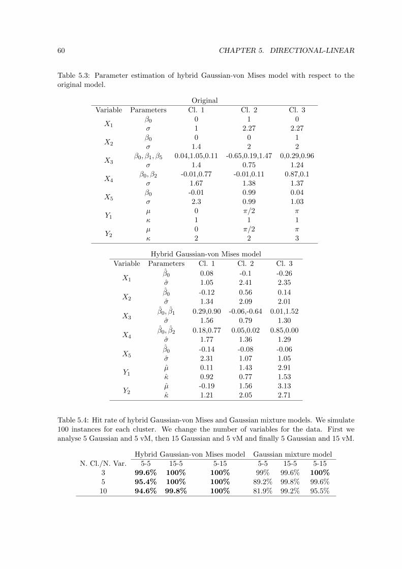
60 CHAPTER 5. DIRECTIONAL-LINEAR
Table 5.3: Parameter estimation of hybrid Gaussian-von Mises model with respect to theoriginal model.
Original
Variable Parameters Cl. 1 Cl. 2 Cl. 3
X1β0 0 1 0σ 1 2.27 2.27
X2β0 0 0 1σ 1.4 2 2
X3β0, β1, β5 0.04,1.05,0.11 -0.65,0.19,1.47 0,0.29,0.96
σ 1.4 0.75 1.24
X4β0, β2 -0.01,0.77 -0.01,0.11 0.87,0.1σ 1.67 1.38 1.37
X5β0 -0.01 0.99 0.04σ 2.3 0.99 1.03
Y1µ 0 π/2 πκ 1 1 1
Y2µ 0 π/2 πκ 2 2 3
Hybrid Gaussian-von Mises model
Variable Parameters Cl. 1 Cl. 2 Cl. 3
X1β0 0.08 -0.1 -0.26σ 1.05 2.41 2.35
X2β0 -0.12 0.56 0.14σ 1.34 2.09 2.01
X3β0, β1 0.29,0.90 -0.06,-0.64 0.01,1.52σ 1.56 0.79 1.30
X4β0, β2 0.18,0.77 0.05,0.02 0.85,0.00σ 1.77 1.36 1.29
X5β0 -0.14 -0.08 -0.06σ 2.31 1.07 1.05
Y1µ 0.11 1.43 2.91κ 0.92 0.77 1.53
Y2µ -0.19 1.56 3.13κ 1.21 2.05 2.71
Table 5.4: Hit rate of hybrid Gaussian-von Mises and Gaussian mixture models. We simulate100 instances for each cluster. We change the number of variables for the data. First weanalyse 5 Gaussian and 5 vM, then 15 Gaussian and 5 vM and finally 5 Gaussian and 15 vM.
Hybrid Gaussian-von Mises model Gaussian mixture modelN. Cl./N. Var. 5-5 15-5 5-15 5-5 15-5 5-15
3 99.6% 100% 100% 99% 99.6% 100%5 95.4% 100% 100% 89.2% 99.8% 99.6%10 94.6% 99.8% 100% 81.9% 99.2% 95.5%
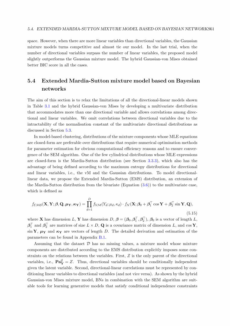
5.4. EXTENDEDMARDIA-SUTTONMIXTUREMODEL BASEDON BAYESIAN NETWORKS61
space. However, when there are more linear variables than directional variables, the Gaussian
mixture models turns competitive and almost tie our model. In the last trial, when the
number of directional variables surpass the number of linear variables, the proposed model
slightly outperforms the Gaussian mixture model. The hybrid Gaussian-von Mises obtained
better BIC score in all the cases.
5.4 Extended Mardia-Sutton mixture model based on Bayesian
networks
The aim of this section is to relax the limitations of all the directional-linear models shown
in Table 3.1 and the hybrid Gaussian-von Mises by developing a multivariate distribution
that accommodates more than one directional variable and allows correlations among direc-
tional and linear variables. We omit correlations between directional variables due to the
intractability of the normalisation constant of the multivariate directional distributions as
discussed in Section 5.3.
In model-based clustering, distributions of the mixture components whose MLE equations
are closed-form are preferable over distributions that require numerical optimisation methods
for parameter estimation for obvious computational efficiency reasons and to ensure conver-
gence of the SEM algorithm. One of the few cylindrical distributions whose MLE expressions
are closed-form is the Mardia-Sutton distribution (see Section 3.3.3), which also has the
advantage of being defined according to the maximum entropy distributions for directional
and linear variables, i.e., the vM and the Gaussian distributions. To model directional-
linear data, we propose the Extended Mardia-Sutton (EMS) distribution, an extension of
the Mardia-Sutton distribution from the bivariate (Equation (3.6)) to the multivariate case,
which is defined as
fEMS(X,Y;β,Q,µY,κY) =D∏d=1
fVM(Yd;µd, κd) · fN (X;β0 + β>1 cos Y + β>2 sin Y,Q),
(5.15)
where X has dimension L, Y has dimension D, β = (β0,β>1 ,β
>2 ), β0 is a vector of length L,
β>1 and β>2 are matrices of size L×D, Q is a covariance matrix of dimension L, and cos Y,
sin Y, µY and κY are vectors of length D. The detailed derivation and estimation of the
parameters can be found in Appendix B.1.
Assuming that the dataset D has no missing values, a mixture model whose mixture
components are distributed according to the EMS distribution explicitly imposes some con-
straints on the relations between the variables. First, Z is the only parent of the directional
variables, i.e., PaGY = Z. Thus, directional variables should be conditionally independent
given the latent variable. Second, directional-linear correlations must be represented by con-
ditioning linear variables to directional variables (and not vice versa). As shown by the hybrid
Gaussian-von Mises mixture model, BNs in combination with the SEM algorithm are suit-
able tools for learning generative models that satisfy conditional independence constraints
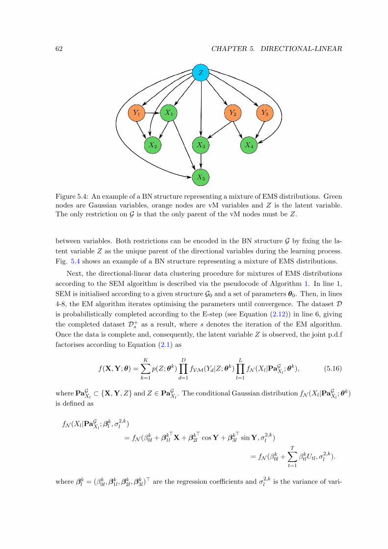
62 CHAPTER 5. DIRECTIONAL-LINEAR
Figure 5.4: An example of a BN structure representing a mixture of EMS distributions. Greennodes are Gaussian variables, orange nodes are vM variables and Z is the latent variable.The only restriction on G is that the only parent of the vM nodes must be Z.
between variables. Both restrictions can be encoded in the BN structure G by fixing the la-
tent variable Z as the unique parent of the directional variables during the learning process.
Fig. 5.4 shows an example of a BN structure representing a mixture of EMS distributions.
Next, the directional-linear data clustering procedure for mixtures of EMS distributions
according to the SEM algorithm is described via the pseudocode of Algorithm 1. In line 1,
SEM is initialised according to a given structure G0 and a set of parameters θ0. Then, in lines
4-8, the EM algorithm iterates optimising the parameters until convergence. The dataset Dis probabilistically completed according to the E-step (see Equation (2.12)) in line 6, giving
the completed dataset D+s as a result, where s denotes the iteration of the EM algorithm.
Once the data is complete and, consequently, the latent variable Z is observed, the joint p.d.f
factorises according to Equation (2.1) as
f(X,Y;θ) =
K∑k=1
p(Z;θk)
D∏d=1
fVM(Yd|Z;θk)
L∏l=1
fN (Xl|PaGXl ;θk), (5.16)
where PaGXl ⊂ {X,Y, Z} and Z ∈ PaGXl . The conditional Gaussian distribution fN (Xl|PaGXl ;θk)
is defined as
fN (Xl|PaGXl ;βkl , σ
2,kl )
= fN (βk0l + βk1l>
X + βk2l>
cos Y + βk3l>
sin Y, σ2,kl )
= fN (βk0l +
T∑t=1
βktlUtl, σ2,kl ).
where βkl = (βk0l,βk1l,β
k2l,β
k3l)> are the regression coefficients and σ2,k
l is the variance of vari-
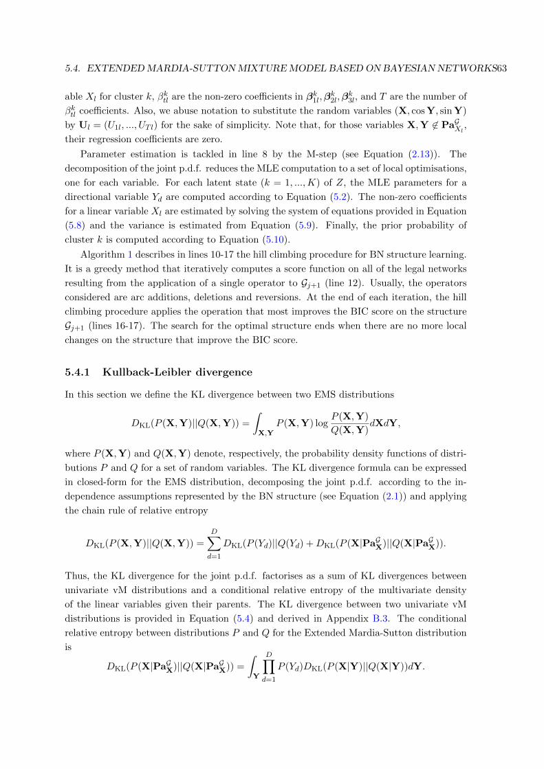
5.4. EXTENDEDMARDIA-SUTTONMIXTUREMODEL BASEDON BAYESIAN NETWORKS63
able Xl for cluster k, βktl are the non-zero coefficients in βk1l,βk2l,β
k3l, and T are the number of
βktl coefficients. Also, we abuse notation to substitute the random variables (X, cos Y, sin Y)
by Ul = (U1l, ..., UT l) for the sake of simplicity. Note that, for those variables X,Y 6∈ PaGXl ,
their regression coefficients are zero.
Parameter estimation is tackled in line 8 by the M-step (see Equation (2.13)). The
decomposition of the joint p.d.f. reduces the MLE computation to a set of local optimisations,
one for each variable. For each latent state (k = 1, ...,K) of Z, the MLE parameters for a
directional variable Yd are computed according to Equation (5.2). The non-zero coefficients
for a linear variable Xl are estimated by solving the system of equations provided in Equation
(5.8) and the variance is estimated from Equation (5.9). Finally, the prior probability of
cluster k is computed according to Equation (5.10).
Algorithm 1 describes in lines 10-17 the hill climbing procedure for BN structure learning.
It is a greedy method that iteratively computes a score function on all of the legal networks
resulting from the application of a single operator to Gj+1 (line 12). Usually, the operators
considered are arc additions, deletions and reversions. At the end of each iteration, the hill
climbing procedure applies the operation that most improves the BIC score on the structure
Gj+1 (lines 16-17). The search for the optimal structure ends when there are no more local
changes on the structure that improve the BIC score.
5.4.1 Kullback-Leibler divergence
In this section we define the KL divergence between two EMS distributions
DKL(P (X,Y)||Q(X,Y)) =
∫X,Y
P (X,Y) logP (X,Y)
Q(X,Y)dXdY,
where P (X,Y) and Q(X,Y) denote, respectively, the probability density functions of distri-
butions P and Q for a set of random variables. The KL divergence formula can be expressed
in closed-form for the EMS distribution, decomposing the joint p.d.f. according to the in-
dependence assumptions represented by the BN structure (see Equation (2.1)) and applying
the chain rule of relative entropy
DKL(P (X,Y)||Q(X,Y)) =D∑d=1
DKL(P (Yd)||Q(Yd) +DKL(P (X|PaGX)||Q(X|PaGX)).
Thus, the KL divergence for the joint p.d.f. factorises as a sum of KL divergences between
univariate vM distributions and a conditional relative entropy of the multivariate density
of the linear variables given their parents. The KL divergence between two univariate vM
distributions is provided in Equation (5.4) and derived in Appendix B.3. The conditional
relative entropy between distributions P and Q for the Extended Mardia-Sutton distribution
is
DKL(P (X|PaGX)||Q(X|PaGX)) =
∫Y
D∏d=1
P (Yd)DKL(P (X|Y)||Q(X|Y))dY.

64 CHAPTER 5. DIRECTIONAL-LINEAR
Given that P (X|Y) and Q(X|Y) are distributed according to a multivariate normal distri-
bution (see Equation (5.15)), the KL divergence is computed according to Equation (5.13).
For the sake of simplicity, we define µR = µQ − µP as
µR = (βQ0 − βP0 ) + (βQ1 − βP1 )>
cos Y + (βQ2 − βP2 )>
sin Y = βR0 + βR1>
cos Y + βR2>
sin Y.
The conditional relative entropy is then computed according to
DKL(P (X|PaGX)||Q(X|PaGX)) =1
2
L∑i,j=1
Σ−1,Qij
[βR0iβ
R0j + 2βR0i
D∑d=1
βR1jdA(κPd )
+D∑d=1
βR1idβR1jd
2
(1 +
I2(κPd )
I0(κPd )
)+
D∑d=1
D∑m6=d
βR1idβR1jmA(κPd )A(κPm) +
D∑d=1
βR2idβR2jd
2
(1−
I2(κPd )
I0(κPd )
)]+
1
2
[Tr(Σ−1,QΣP )− L+ ln
|ΣQ||ΣP |
].
where βR1id and βR2id are the d-th element of vectors βR1i and βR2i of variable Xi; βR0i, β
R1i and
βR2i are the coefficients of the conditional mean corresponding to the linear variable Xi, i.e.,
the i-th elements of vectors βR0 , βR1 and βR2 ; Σ−1,Qij is the element at the i-th row and j-
th column of the matrix Σ−1,Q, and κPd is the concentration parameter of the distribution
P (Yd) = fVM(Yd;µPd , κ
Pd ). A more detailed description of the procedure to obtain the above
expression is provided in Appendix B.4.1. In the case of the EMS distribution we did not
develop the derivation of the BD because it has not close-form equations.
5.4.2 Experiments
The main goal of model-based clustering is to recover the underlying distribution that gener-
ated the dataset used to learn the model. We compared the performance between our model
and the hybrid Gaussian-von Mises model introduced in Section 5.3 in this task measuring
the similarity of the models learnt by both approaches with respect to artificially generated
BNs. We considered the hybrid Gaussian-von Mises model for the evaluation because, to the
best of our knowledge, it is the only model in the state of the art that can cluster several
directional and linear variables.
The artificial BNs were randomly generated according to the procedure presented in
[Kalisch and Buhlmann, 2007]. Concretely, the structure G of the artificial BNs was defined
by an adjacency matrix A full of zeros with a fixed ordering of the variables such that the
directional variables were placed before the linear variables. Then, every entry in the lower
triangle of A involving at least one linear variable was replaced by the result of a Bernoulli
trial with a success probability of 0.4. Each success represented an edge of the structure
G. From matrix A the parameters of each mixture component were generated randomly as
follow:
� Each directional variable Yd ∈ Y was assumed to have a vM distribution with mean
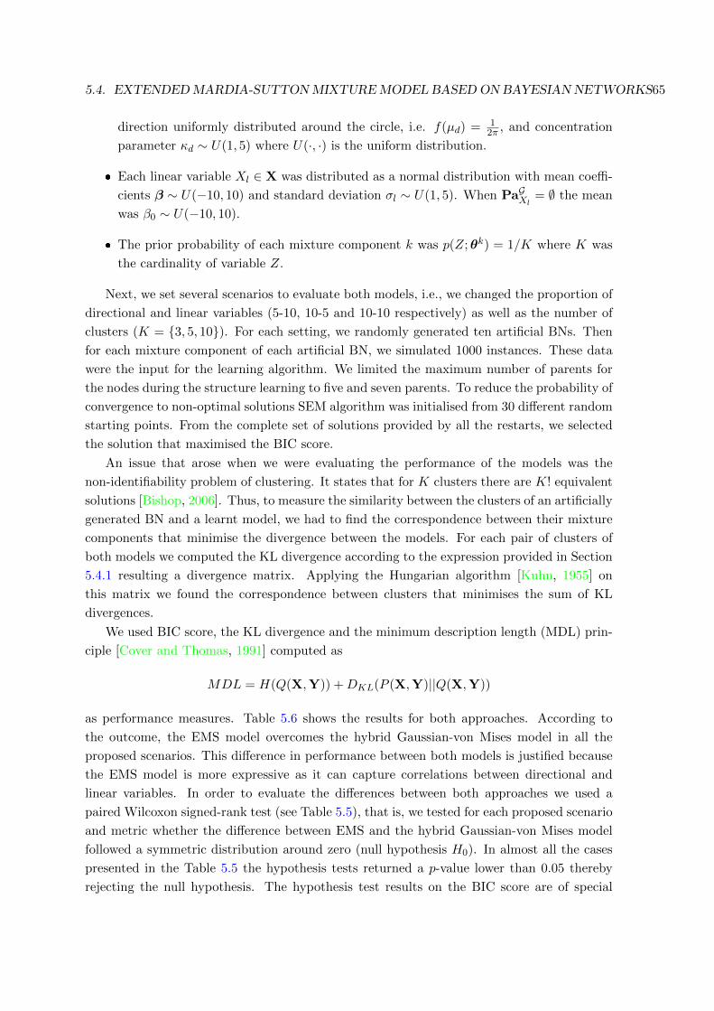
5.4. EXTENDEDMARDIA-SUTTONMIXTUREMODEL BASEDON BAYESIAN NETWORKS65
direction uniformly distributed around the circle, i.e. f(µd) = 12π , and concentration
parameter κd ∼ U(1, 5) where U(·, ·) is the uniform distribution.
� Each linear variable Xl ∈ X was distributed as a normal distribution with mean coeffi-
cients β ∼ U(−10, 10) and standard deviation σl ∼ U(1, 5). When PaGXl = ∅ the mean
was β0 ∼ U(−10, 10).
� The prior probability of each mixture component k was p(Z;θk) = 1/K where K was
the cardinality of variable Z.
Next, we set several scenarios to evaluate both models, i.e., we changed the proportion of
directional and linear variables (5-10, 10-5 and 10-10 respectively) as well as the number of
clusters (K = {3, 5, 10}). For each setting, we randomly generated ten artificial BNs. Then
for each mixture component of each artificial BN, we simulated 1000 instances. These data
were the input for the learning algorithm. We limited the maximum number of parents for
the nodes during the structure learning to five and seven parents. To reduce the probability of
convergence to non-optimal solutions SEM algorithm was initialised from 30 different random
starting points. From the complete set of solutions provided by all the restarts, we selected
the solution that maximised the BIC score.
An issue that arose when we were evaluating the performance of the models was the
non-identifiability problem of clustering. It states that for K clusters there are K! equivalent
solutions [Bishop, 2006]. Thus, to measure the similarity between the clusters of an artificially
generated BN and a learnt model, we had to find the correspondence between their mixture
components that minimise the divergence between the models. For each pair of clusters of
both models we computed the KL divergence according to the expression provided in Section
5.4.1 resulting a divergence matrix. Applying the Hungarian algorithm [Kuhn, 1955] on
this matrix we found the correspondence between clusters that minimises the sum of KL
divergences.
We used BIC score, the KL divergence and the minimum description length (MDL) prin-
ciple [Cover and Thomas, 1991] computed as
MDL = H(Q(X,Y)) +DKL(P (X,Y)||Q(X,Y))
as performance measures. Table 5.6 shows the results for both approaches. According to
the outcome, the EMS model overcomes the hybrid Gaussian-von Mises model in all the
proposed scenarios. This difference in performance between both models is justified because
the EMS model is more expressive as it can capture correlations between directional and
linear variables. In order to evaluate the differences between both approaches we used a
paired Wilcoxon signed-rank test (see Table 5.5), that is, we tested for each proposed scenario
and metric whether the difference between EMS and the hybrid Gaussian-von Mises model
followed a symmetric distribution around zero (null hypothesis H0). In almost all the cases
presented in the Table 5.5 the hypothesis tests returned a p-value lower than 0.05 thereby
rejecting the null hypothesis. The hypothesis test results on the BIC score are of special
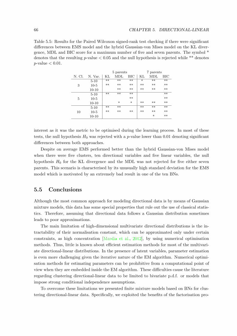
66 CHAPTER 5. DIRECTIONAL-LINEAR
Table 5.5: Results for the Paired Wilcoxon signed-rank test checking if there were significantdifferences between EMS model and the hybrid Gaussian-von Mises model on the KL diver-gence, MDL and BIC score for a maximum number of five and seven parents. The symbol *denotes that the resulting p-value < 0.05 and the null hypothesis is rejected while ** denotesp-value < 0.01.
5 parents 7 parentsN. Cl. N. Var. KL MDL BIC KL MDL BIC
35-10 ** ** ** * ** **10-5 ** ** ** ** ** **10-10 ** ** ** ** **
55-10 ** ** ** **10-5 ** **10-10 * * ** ** **
105-10 ** ** ** ** **10-5 ** ** ** ** ** **10-10 * **
interest as it was the metric to be optimised during the learning process. In most of these
tests, the null hypothesis H0 was rejected with a p-value lower than 0.01 denoting significant
differences between both approaches.
Despite on average EMS performed better than the hybrid Gaussian-von Mises model
when there were five clusters, ten directional variables and five linear variables, the null
hypothesis H0 for the KL divergence and the MDL was not rejected for five either seven
parents. This scenario is characterised by its unusually high standard deviation for the EMS
model which is motivated by an extremely bad result in one of the ten BNs.
5.5 Conclusions
Although the most common approach for modeling directional data is by means of Gaussian
mixture models, this data has some special properties that rule out the use of classical statis-
tics. Therefore, assuming that directional data follows a Gaussian distribution sometimes
leads to poor approximations.
The main limitation of high-dimensional multivariate directional distributions is the in-
tractability of their normalisation constant, which can be approximated only under certain
constraints, as high concentration [Mardia et al., 2012], by using numerical optimisation
methods. Thus, little is known about efficient estimation methods for most of the multivari-
ate directional-linear distributions. In the presence of latent variables, parameter estimation
is even more challenging given the iterative nature of the EM algorithm. Numerical optimi-
sation methods for estimating parameters can be prohibitive from a computational point of
view when they are embedded inside the EM algorithm. These difficulties cause the literature
regarding clustering directional-linear data to be limited to bivariate p.d.f. or models that
impose strong conditional independence assumptions.
To overcome these limitations we presented finite mixture models based on BNs for clus-
tering directional-linear data. Specifically, we exploited the benefits of the factorisation pro-

5.5. CONCLUSIONS 67
vided by the structure of the BNs to get closed-form equations for the maximisation step of
the EM algorithm. Additionally, we also learned the conditional dependence relations among
variables according to the SEM algorithm. This allow us to learn models even when the
data availability is scarce. We also developed a multivariate extension of the Mardia-Sutton
distribution, as well as the closed-form expressions for similarity measures between clusters as
the KL divergence and the BD distance. The proposed multivariate distribution relaxes the
independence constraints among directional and linear variables of previous directional-linear
models applied in clustering, allowing for any number of directional-linear correlations and
avoiding approximate estimation of the parameters.
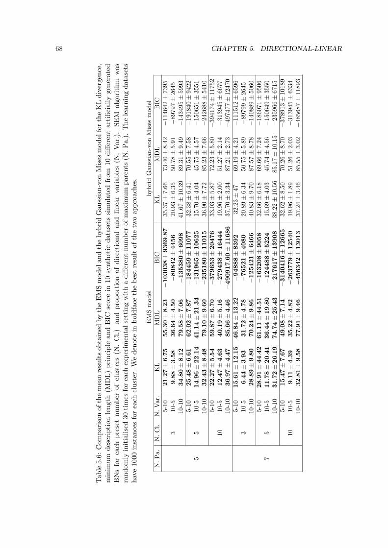
68 CHAPTER 5. DIRECTIONAL-LINEAR
Tab
le5.
6:C
omp
aris
onof
the
mea
nre
sult
sob
tain
edby
the
EM
Sm
od
elan
dth
ehyb
rid
Gauss
ian-v
on
Mis
esm
od
elfo
rth
eK
Ld
iver
gen
ce,
min
imu
md
escr
ipti
onle
ngt
h(M
DL
)p
rin
cip
lean
dB
ICsc
ore
in10
synth
etic
dat
aset
ssi
mu
late
dfr
om
10
diff
eren
tart
ifici
all
ygen
erate
dB
Ns
for
each
pre
set
nu
mb
erof
clu
ster
s(N
.C
l.)
and
pro
por
tion
ofd
irec
tion
alan
dli
nea
rva
riab
les
(N.
Var.
).S
EM
alg
ori
thm
was
ran
dom
lyin
itia
lise
d30
tim
esfo
rea
chex
per
imen
tal
sett
ing
wit
ha
diff
eren
tnu
mb
erof
maxim
um
pare
nts
(N.
Pa.)
.T
he
learn
ing
data
sets
hav
e10
00in
stan
ces
for
each
clu
ster
.W
ed
enot
ein
bol
dfa
ceth
eb
est
resu
ltof
the
two
ap
pro
ach
es.
EM
Sm
od
elhybri
dG
auss
ian
-von
Mis
esm
odel
N.
Pa.
N.
Cl.
N.
Var
.K
LM
DL
BIC
KL
MD
LB
IC
5
35-
10
21.2
7±
6.7
555.3
0±
8.2
3−
103038±
9369.8
735.3
7±
7.66
73.4
0±
8.42
−11
4642±
7395
10-5
9.8
8±
3.5
836.6
4±
4.5
0−
80842±
4456
20.9
3±
6.35
50.7
8±
5.91
−89
797±
2645
10-1
034.8
0±
8.1
279.5
8±
7.0
6−
135380±
6098
41.6
7±
10.3
989.3
1±
9.49
−14
3495±
5993
55-
10
25.4
8±
6.6
162.0
2±
7.8
7−
184459±
11077
32.3
8±
6.41
70.5
5±
7.58
−19
1840±
9422
10-5
14.9
6±
22.1
441.1
4±
21.3
4−
131965±
10625
15.7
0±
4.04
45.7
5±
4.57
−15
0651±
3551
10-1
032.4
3±
8.4
879.1
0±
9.6
0−
235180±
11015
36.9
0±
7.72
85.2
3±
7.66
−24
2688±
5410
105-
1022.2
7±
5.5
459.8
7±
6.7
0−
379653±
20476
33.0
3±
5.87
72.2
3±
5.80
−39
4174±
1175
210
-512.4
7±
4.6
340.1
9±
5.1
6−
279438±
16444
19.9
6±
2.00
51.2
7±
2.14
−31
3945±
6677
10-1
036.9
7±
4.4
785.6
6±
4.4
6−
490917.6
0±
11686
37.7
0±
3.34
87.2
1±
2.73
−49
7477±
1247
0
7
35-
10
15.6
1±
12.1
546.8
4±
13.2
2−
94888±
8392
32.2
3±
4769.1
9±
4.21
−11
1512±
6596
10-5
6.4
4±
3.9
331.7
2±
4.7
8−
76521±
4080
20.8
9±
6.34
50.7
5±
5.89
−89
799±
2645
10-1
028.8
9±
9.8
070.2
4±
9.8
6−
125421±
6466
40.8
3±
9.70
87.5
7±
8.78
−14
0889±
5060
55-
10
28.9
1±
44.4
261.1
1±
44.5
1−
163208±
9058
32.6
6±
6.18
69.6
6±
7.24
−18
6071±
9506
10-5
11.7
8±
20.4
136.4
4±
19.8
0−
124488±
5224
15.6
9±
4.03
45.7
4±
4.56
−15
0649±
3550
10-1
031.7
2±
26.1
974.7
4±
25.4
3−
217617±
13908
38.2
2±
10.5
685.1
7±
10.1
5−
2359
66±
6715
105-
1015.4
7±
7.6
749.0
8±
7.1
4−
3140416±
12665
32.6
2±
8.50
70.2
6±
8.70
−37
8913±
1018
910
-59.1
1±
4.3
935.2
2±
4.8
2−
263779±
12540
19.9
6±
1.89
51.2
6±
2.03
−31
3945±
6334
10-1
032.8
1±
9.5
877.9
1±
9.4
6−
456342±
13013
37.2
4±
3.46
85.5
5±
3.02
−48
5687±
1189
3
Part IV
CONTRIBUTIONS TO
NEUROSCIENCE
69

Chapter 63D morphology-based clustering
and simulation of human pyramidal
cell dendritic spines
6.1 Introduction
Dendritic spines present a large diversity of sizes and morphologies, especially in the human
cortex [Benavides-Piccione et al., 2012]. The most accepted categorisation of the dendritic
spines based on their morphology was proposed by Peters and Kaiserman-Abramof [1970]
that defines three basic classes -thin, mushroom and stubby spines- and an additional group
-filopodium. However, Arellano et al. [2007], Loewenstein et al. [2015] and Tønnesen et al.
[2014] discuss if this variety of shapes is the result of a continuum of morphologies instead
of concrete categories. Recently, both Bokota et al. [2016] and Ghani et al. [2016] applied
automatic clustering techniques over 2D dendritic spine representations to objectively address
this debate. They concluded that some spines clearly belong to Peters and Kaiserman-
Abramof’s classes but the rest cannot be ascribed to any category because their morphology
present transitions between shapes.
Nevertheless, the geometry of spines can be more accurately determined by means of
3D reconstructions, since many morphological features are not taken into account in 2D.
Ideally, 3D reconstruction using electron microscopy serial sections is the gold standard to
obtain accurate estimations of the geometry of spines. However, a relatively low number of
spines (at best in the order of a few hundreds) can be reconstructed in 3D using electron
microscopy in a reasonable time period, and these reconstructions can only be carried out in
small segments of the dendritic arbor of the neurons. Furthermore, the quality of electron
microscopy when using human brain tissue is usually suboptimal due to technical constraints.
On the contrary, fluorescent labeling of neurons and the use of high power reconstruction with
confocal microscopy (or other techniques) allow the visualization of thousands of spines with
high quality along the dendritic arbor (apical and basal dendrites). Thus, in this chapter, we
71
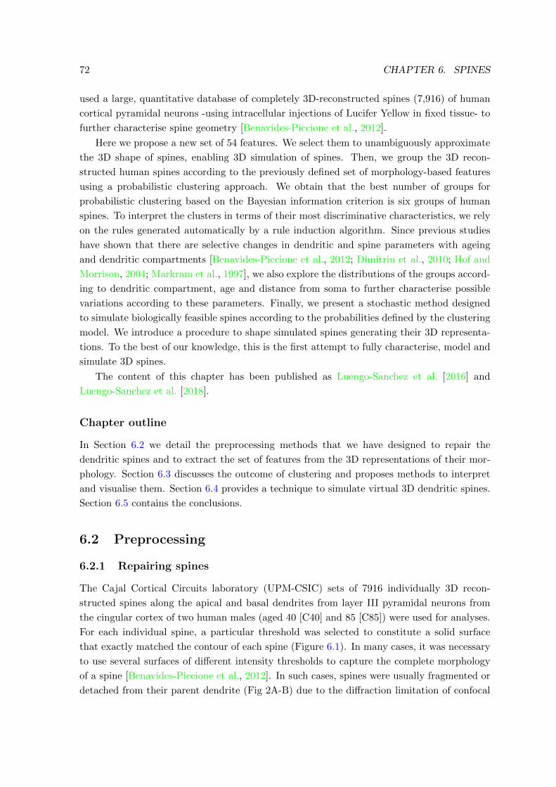
72 CHAPTER 6. SPINES
used a large, quantitative database of completely 3D-reconstructed spines (7,916) of human
cortical pyramidal neurons -using intracellular injections of Lucifer Yellow in fixed tissue- to
further characterise spine geometry [Benavides-Piccione et al., 2012].
Here we propose a new set of 54 features. We select them to unambiguously approximate
the 3D shape of spines, enabling 3D simulation of spines. Then, we group the 3D recon-
structed human spines according to the previously defined set of morphology-based features
using a probabilistic clustering approach. We obtain that the best number of groups for
probabilistic clustering based on the Bayesian information criterion is six groups of human
spines. To interpret the clusters in terms of their most discriminative characteristics, we rely
on the rules generated automatically by a rule induction algorithm. Since previous studies
have shown that there are selective changes in dendritic and spine parameters with ageing
and dendritic compartments [Benavides-Piccione et al., 2012; Dimitriu et al., 2010; Hof and
Morrison, 2004; Markram et al., 1997], we also explore the distributions of the groups accord-
ing to dendritic compartment, age and distance from soma to further characterise possible
variations according to these parameters. Finally, we present a stochastic method designed
to simulate biologically feasible spines according to the probabilities defined by the clustering
model. We introduce a procedure to shape simulated spines generating their 3D representa-
tions. To the best of our knowledge, this is the first attempt to fully characterise, model and
simulate 3D spines.
The content of this chapter has been published as Luengo-Sanchez et al. [2016] and
Luengo-Sanchez et al. [2018].
Chapter outline
In Section 6.2 we detail the preprocessing methods that we have designed to repair the
dendritic spines and to extract the set of features from the 3D representations of their mor-
phology. Section 6.3 discusses the outcome of clustering and proposes methods to interpret
and visualise them. Section 6.4 provides a technique to simulate virtual 3D dendritic spines.
Section 6.5 contains the conclusions.
6.2 Preprocessing
6.2.1 Repairing spines
The Cajal Cortical Circuits laboratory (UPM-CSIC) sets of 7916 individually 3D recon-
structed spines along the apical and basal dendrites from layer III pyramidal neurons from
the cingular cortex of two human males (aged 40 [C40] and 85 [C85]) were used for analyses.
For each individual spine, a particular threshold was selected to constitute a solid surface
that exactly matched the contour of each spine (Figure 6.1). In many cases, it was necessary
to use several surfaces of different intensity thresholds to capture the complete morphology
of a spine [Benavides-Piccione et al., 2012]. In such cases, spines were usually fragmented or
detached from their parent dendrite (Fig 2A-B) due to the diffraction limitation of confocal

6.2. PREPROCESSING 73
Table 6.1: Number and percentage of spines after repair by their dendritic compartment andage.
Prob./Cl. C40 C85 Sum
Apical 1,893 (26%) 1,057 (14%) 2,950 (40%)Basal 2,500 (34%) 1,847 (26%) 4,347 (60%)Sum 4,393 (60%) 2,904 (40%) 7,297 (100%)
microscopy. Therefore, they had to be repaired by means of a novel semi-supervised mesh
processing algorithm which generated a new dataset of corrected spines.
We addressed the task of repairing spines by means of a semi-automatic mesh processing
algorithm (Fig. 6.2A). The procedure started by identifying fragmented spines. A spine
was fragmented if there was no path between every pair of vertices on the surface of the 3D
mesh, and all the vertices belonged to a closed mesh. If this was the case, fragmentation
was repaired by applying a closing morphological operator to each spine individually. This
operator requires a binary image as input, and therefore 3D meshes were voxelized [Patil and
Ravi, 2005]. As a result of applying the closing operator to each voxel of the volumetric spine
using a sphere as a structuring element, fragments were joined to form a single body. The
marching cubes algorithm [Lorensen and Cline, 1987] recovered the mesh representation from
the volumetric image of the repaired spine.
The repair process was continued by connecting spines to dendrites by means of spine
path reconstruction (Figure 6.2B). Several points were created to attach the spine to the
dendrite, using the measurement point tool in Imaris software. These are considered to be
the spine insertion points. In those cases where the created spine surface did not reach the
dendritic shaft, the insertion point was placed directly on the dendritic shaft where the spine
emerged from the shaft, while rotating the image in 3D (Figure 6.1G). Spine reconstruction
was applied to any spines whose insertion point was not on the surface of the mesh. This
step in the repair process consists of filling the gap between the closest vertex of the spine
to the insertion point and the insertion point according to an iterative process that grew
the missing base of the spine. Specifically, each detached spine was oriented so that both
points bounding the gap were aligned with the z-axis. Then, the mesh of each spine was
voxelized. Each voxel slice perpendicular to the z-axis between the spine and the insertion
point was filled with the result of applying a 2D Gaussian filter to the slice immediately above.
The mesh representation of the completely repaired spine was recovered from the volumetric
representation by the marching cubes algorithm. Finally, we smoothed the triangular mesh
with a curvature flow technique [Desbrun et al., 1999]. Those spines that were extremely
fragmented, far removed from the dendrite or significantly deferred from their original shape
were discarded. As a result, the original set of 7,916 spines yielded 7,297 (92.18%) spines.
The number and percentage of spines after repair by their dendritic compartment and age
can be found in Table 6.1.
For the repair process, the insertion point of each spine was manually marked, approxi-
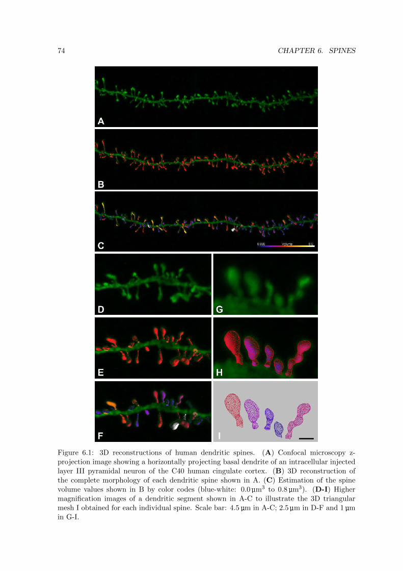
74 CHAPTER 6. SPINES
Figure 6.1: 3D reconstructions of human dendritic spines. (A) Confocal microscopy z-projection image showing a horizontally projecting basal dendrite of an intracellular injectedlayer III pyramidal neuron of the C40 human cingulate cortex. (B) 3D reconstruction ofthe complete morphology of each dendritic spine shown in A. (C) Estimation of the spinevolume values shown in B by color codes (blue-white: 0.0 µm3 to 0.8 µm3). (D-I) Highermagnification images of a dendritic segment shown in A-C to illustrate the 3D triangularmesh I obtained for each individual spine. Scale bar: 4.5 µm in A-C; 2.5 µm in D-F and 1 µmin G-I.

6.2. PREPROCESSING 75
Figure 6.2: Spine repair process and multiresolutional Reeb graph computation. Spines arecolored with a gradient whereby the closest points to the insertion point were colored greenand the furthest points were colored purple. (A) Example of a fragmented spine. Thefragmentation problem is solved by applying the closing morphological operator, and thespine is completely connected. (B) Example of the reconstruction of a spine detached fromits dendritic shaft. The spine was oriented so as to align the insertion point and its closestvertex with the z-axis. The gap between the spine and the dendritic shaft is filled by meansof an iterative process starting from the base of the spine. This resulted in the growth of themissing neck. (C) Geodesic distance computation from the insertion point. The black linedenotes the shortest path from the insertion point to an arbitrary point on the surface ofthe spine. (D) The domain of the geodesic distance on the surface of the spine was dividedinto seven regions. (E) Regions and segments between curves provide enough informationto reconstruct an approximation of the surface. Features extracted from these regions andsegments must conform a complete set of spine topology to provide for a proper computersimulation. (F) Curves were approximated by the best fitting plane resulting in ellipses thatimprove the characterisation and interpretation of the geometry of the spine. Features werecomputed on this final 3D representation.

76 CHAPTER 6. SPINES
mately at the center of the created spine surface side that was in contact with the dendritic
shaft. In those cases where the created spine surface did not reach the dendritic shaft, the
insertion point was placed directly on the dendritic shaft where the spine emerged from the
shaft, while rotating the image in 3D (Figure 6.1G). The insertion point was useful for repair-
ing the detached spines and computing a multiresolutional Reeb graph for feature extraction.
6.2.2 Feature extraction
Given 3D meshes representing the surface of the spines, our goal was to extract a set
of morphological features providing enough information to reconstruct an approximation
of their original shapes. Our work was partially inspired by the concept of multiresolu-
tional Reeb graph (MRG) [Tangelder and Veltkamp, 2008] and its particular implemen-
tation in [Hilaga et al., 2001], a technique that constructs a graph from a 3D geometric
model to describe its topology (Figure 6.2C-F). This approach partitions a triangular mesh
into regions based on the value of a function µ(·). This function should preferably be the
geodesic distance, i.e., the shortest path between two points of the mesh along the surface
because it is invariant to translation and rotation and is robust against mesh simplifica-
tion and subdivision. We computed geodesic distance from the insertion point of the spine
to each vertex of the mesh (Figure 6.2C). The domain of µ(·) was divided into K = 7
equal length intervals, where ri indicates the beginning and the end of each region such that
r0 =[0, 1
Kα], r1 =
(1Kα,
2Kα], . . . , rK−1 =
(K−1K α, α
], where α is maxµ(·). This means that
each of the vertices in the triangular mesh was allocated to a particular region depending
on its evaluation function µ(·) (Figure 6.2D-E). At each region i, the curves defining the top
and bottom bounds were assumed to be ellipses contained in the best fitting plane computed
using principal component analysis. We denote Ti and Bi the top and the bottom ellipses of
each region i respectively. Thus, each region provided a local description of the morphology
while the combination of the information of all regions represented a global characterisation
of the spine. Representing a spine as a set of ellipses allows us to capture its most relevant
morphological aspects while spurious details are avoided.
The proposed set of 54 features must unambiguously describe the placement and orienta-
tion of all the ellipses that characterise the geometry of a spine, i.e., there must be a unique
correspondence between an assignment to the features and a 3D spine. If this condition is
fulfilled, then the features should capture all of the relevant geometrical information of the
spine, and consequently any morphometric measure can be computed from the set of features.
To achieve this, at each region i a set of features was computed according to their ellipses Ti
and Bi. Since the surface was required to be continuous coherence constraints were imposed
on adjacent regions: ∀i, 1 < i < K + 1, BRi = TRi−1, B
ri = T ri−1. Thus, to satisfy the previous
condition the following features were considered to characterise the spine (Figure 6.3)
� Height (|hi|): This variable measures the length of the vector hi between the centroids
of two consecutive ellipses. The higher the value of this variable, the longer the spine
in that region.
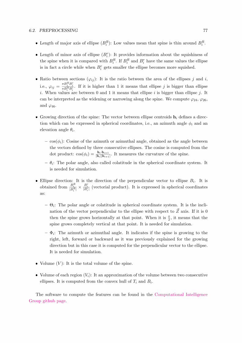
6.2. PREPROCESSING 77
� Length of major axis of ellipse (BRi ): Low values mean that spine is thin around BR
i .
� Length of minor axis of ellipse (Bri ): It provides information about the squishiness of
the spine when it is compared with BRi . If BR
i and Bri have the same values the ellipse
is in fact a circle while when Bri gets smaller the ellipse becomes more squished.
� Ratio between sections (ϕij): It is the ratio between the area of the ellipses j and i,
i.e., ϕij =πBRj B
rj
πBRi Bri. If it is higher than 1 it means that ellipse j is bigger than ellipse
i. When values are between 0 and 1 it means that ellipse i is bigger than ellipse j. It
can be interpreted as the widening or narrowing along the spine. We compute ϕ24, ϕ26,
and ϕ46.
� Growing direction of the spine: The vector between ellipse centroids hi defines a direc-
tion which can be expressed in spherical coordinates, i.e., an azimuth angle φi and an
elevation angle θi.
– cos(φi): Cosine of the azimuth or azimuthal angle, obtained as the angle between
the vectors defined by three consecutive ellipses. The cosine is computed from the
dot product: cos(φi) = hi·hi+1
|hi||hi+1| . It measures the curvature of the spine.
– θi: The polar angle, also called colatitude in the spherical coordinate system. It
is needed for simulation.
� Ellipse direction: It is the direction of the perpendicular vector to ellipse Bi. It is
obtained fromBRi|BRi |× Bri|Bri |
(vectorial product). It is expressed in spherical coordinates
as:
– Θi: The polar angle or colatitude in spherical coordinate system. It is the incli-
nation of the vector perpendicular to the ellipse with respect to ~Z axis. If it is 0
then the spine grows horizontally at that point. When it is π2 , it means that the
spine grows completely vertical at that point. It is needed for simulation.
– Φi: The azimuth or azimuthal angle. It indicates if the spine is growing to the
right, left, forward or backward as it was previously explained for the growing
direction but in this case it is computed for the perpendicular vector to the ellipse.
It is needed for simulation.
� Volume (V ): It is the total volume of the spine.
� Volume of each region (Vi): It an approximation of the volume between two consecutive
ellipses. It is computed from the convex hull of Ti and Bi.
The software to compute the features can be found in the Computational Intelligence
Group github page.
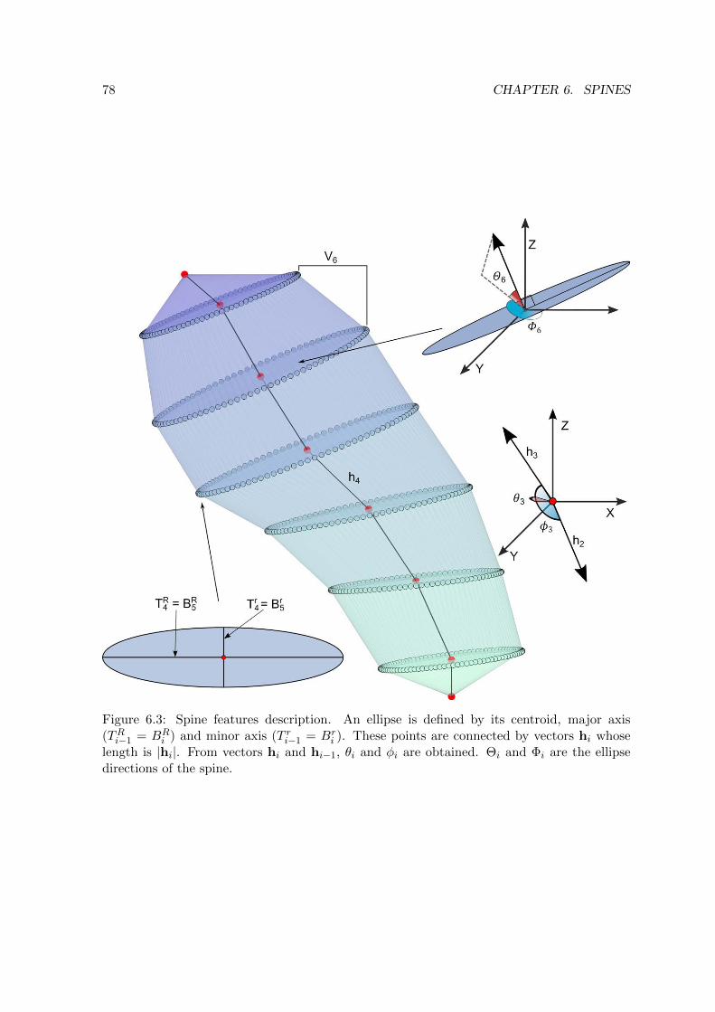
78 CHAPTER 6. SPINES
Figure 6.3: Spine features description. An ellipse is defined by its centroid, major axis(TRi−1 = BR
i ) and minor axis (T ri−1 = Bri ). These points are connected by vectors hi whose
length is |hi|. From vectors hi and hi−1, θi and φi are obtained. Θi and Φi are the ellipsedirections of the spine.

6.3. CLUSTERING 79
Table 6.2: Number of spines whose maximum probability p∗ of belonging to a cluster isgreater than a threshold. The total number of spines for each cluster is specified betweenparentheses. Column 1 establishes a threshold probability. Each cell denotes the numberof spines that belong to its column cluster with a probability greater than is indicated byits row. For example, 953 spines out of the 1,025 grouped in Cluster 1 had a maximumprobability p∗ greater than 0.99.
Prob./Cl.Cluster 1(1,025)
Cluster 2(1,588)
Cluster 3(1,273)
Cluster 4(1,454)
Cluster 5(1,264)
Cluster 6(693)
0.99 72 124 163 165 109 450.9 30 30 44 50 38 140.8 17 13 25 29 20 110.7 12 7 16 13 10 60.6 9 3 5 6 4 30.5 0 0 0 0 0 0
6.3 Clustering
To find groups of spines, we applied a Gaussian mixture model1 approach for model-based
clustering which assigned spines to six clusters according to the Bayesian information criterion
(BIC) (Fig 6.4A and Sections 2.4.3.3 and 2.5). Our approach, based on probabilistic cluster-
ing, assigned a probability distribution (p1, ..., p6) of belonging to each of the six clusters to
each spine, where pi is the probability of belonging to cluster (pi ∈ [0, 1],∑
i pi = 1). Further-
more, we counted the number of spines whose maximum probability, p∗ = max{p1, ..., p6},was lower than a given threshold (Table 6.2). We found that the membership probabil-
ity of most of the spines was greater than 0.99 and clearly belonged to a cluster, whereas
a very small number were more scattered and, consequently, their membership was not so
clear. Therefore, we can conclude that with this set of features most of spines had very high
membership probabilities.
6.3.1 Cluster interpretation and visualization
To gain a deeper insight into the characterisation of each group unveiled by the probabilistic
clustering, we identified the most representative features for each cluster. The process was
based on the generation of classification rules according to the RIPPER algorithm [Cohen,
1995] with the implementation included in the collection of algorithms of Weka, a software for
machine learning tasks [Hall et al., 2009]. The spines were crisply assigned to a unique cluster
by selecting the most probable cluster for each spine. Then, RIPPER generated discriminative
rules for each cluster, turning the problem into a binary supervised classification problem
which pitched each cluster label against the rest. SMOTE [Chawla et al., 2002] was applied
1At this point we want to clarify that we chose the Gaussian mixture model because this study wasperformed before we developed the directional-linear mixture models presented in Chapter 5. Therefore, weconsidered that the Gaussian mixture model was a reasonable option given its computational tractability andits suitability to approximate any multivariate p.d.f. given enough components.
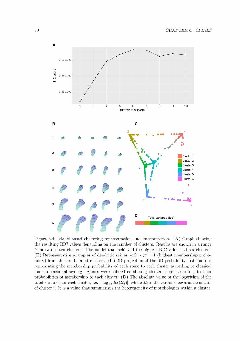
80 CHAPTER 6. SPINES
Figure 6.4: Model-based clustering representation and interpretation. (A) Graph showingthe resulting BIC values depending on the number of clusters. Results are shown in a rangefrom two to ten clusters. The model that achieved the highest BIC value had six clusters.(B) Representative examples of dendritic spines with a p∗ = 1 (highest membership proba-bility) from the six different clusters. (C) 2D projection of the 6D probability distributionsrepresenting the membership probability of each spine to each cluster according to classicalmultidimensional scaling. Spines were colored combining cluster colors according to theirprobabilities of membership to each cluster. (D) The absolute value of the logarithm of thetotal variance for each cluster, i.e., | log10 det(Σi)|, where Σi is the variance-covariance matrixof cluster i. It is a value that summarizes the heterogeneity of morphologies within a cluster.

6.3. CLUSTERING 81
as a pre-processing step before running RIPPER to avoid bias and deal with the unbalanced
distribution of instances arising from data splitting (one cluster versus the rest). SMOTE
is a technique for adjusting the class distribution so that the set of observations of the least
represented class is resampled. We forced RIPPER to classify using a unique rule to improve
the interpretability of each cluster, highlighting its most discriminative features. However,
a single rule cannot be regarded as enough to characterise all the spines within a cluster
because it is unable to capture all the relations between the variables defined by the model-
based clustering. The result was that each cluster was characterised by only one, two or three
observable features (Figure 6.5). The discriminative rules are available in Appendix A. An
example of the representative spines of the six clusters is shown in Figure 6.4B. The rules
generated by RIPPER when it comes to classify the spines according to their cluster label,
with their accuracy between parentheses, may be summarised as:
� Cluster 1: The height of the spines is extremely low in region 2. (92.94%).
� Cluster 2: Spines with a low curvature across regions 4, 5 and 6 and a small volume in
region 7 (80.90%).
� Cluster 3: These spines have a medium-small volume, a low curvature across regions 2
and 3 and the area of their 6-th ellipse area may not be more than double or less than
half of the area of their 4-th ellipse (75.89%).
� Cluster 4: Their volume is high in region 4 and the 6-th ellipse has a smaller area than
the 4-th (82.16%).
� Cluster 5: Groups spines whose height in region 2 is high and whose 6-th ellipse has an
area that is almost equal to or greater than that of the 4-th region (81.95%).
� Cluster 6: Contains the spines with a large volume in region 7 (70.68%).
The diversity of morphologies within a cluster was estimated by computing the total
variance for each cluster. Figure 6.4D shows that Cluster 2 has the lowest total variance,
denoting similarity among its spines, whereas variance in Cluster 6 stands well above that of
the other clusters, suggesting more heterogeneity.
To improve cluster visualization and interpretation, the distances between the member-
ship probabilities (p1, ..., p6) of the spines in a 6D space were projected to 2D according to
multidimensional scaling (see Figure 6.4C). To achieve this goal, distances between each pair
of multivariate Gaussians defined by the clusters were calculated according to the BD [Abou-
Moustafa and Ferrie, 1995] (see Equation (5.14)). Based on this measure, we were then able to
project the above distances, originally in a 6D space, onto a 2D space using multidimensional
scaling [Torgerson, 1958]. Thus, spines were placed and colored in this space in proportion to
the probability of their belonging to each cluster. Accordingly, “intermediate” spines whose
membership probabilities were distributed evenly across several clusters have a mixture of
colors. In this representation, we find that most of the points are clearly assigned to a cluster,

82 CHAPTER 6. SPINES
Figure 6.5: Graphical representations of the main features that characterise each cluster ofspines. Representative examples of the spines of each cluster have been rescaled to improvethe visualization of their characteristics. The actual proportions between spines are shownin 6.4B. (A) The height of the spines that belong to Cluster 1 is extremely low in region2. (B) Cluster 2 includes spines with a low curvature across regions 4, 5 and 6 and a smallvolume in region 7. (C) Spines that were assigned to Cluster 3 have a medium-small volume,a low curvature across regions 2 and 3 and the area of their 6th ellipse area may not be morethan double or less than half of the area of their 4th ellipse. (D) The volume of the spines inCluster 4 is high in region 4 and the 6th ellipse has a smaller area than the 4th. (E) Cluster5 groups spines whose height in region 2 is high and whose 6th ellipse has an area that isalmost equal to or greater than that of the 4th region. (F) Cluster 6 contains the spines witha large volume in region 7.
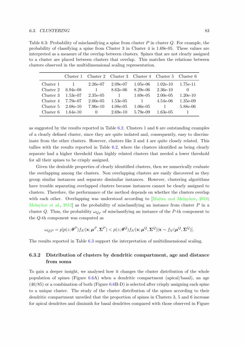
6.3. CLUSTERING 83
Table 6.3: Probability of misclassifying a spine from cluster P in cluster Q. For example, theprobability of classifying a spine from Cluster 3 in Cluster 4 is 1.69e-05. These values areinterpreted as a measure of the overlap between clusters. Spines that are not clearly assignedto a cluster are placed between clusters that overlap. This matches the relations betweenclusters observed in the multidimensional scaling representation.
Cluster 1 Cluster 2 Cluster 3 Cluster 4 Cluster 5 Cluster 6
Cluster 1 1 2.26e-07 2.09e-07 1.05e-06 1.02e-10 1.75e-11Cluster 2 6.94e-08 1 8.62e-06 8.29e-06 2.36e-10 0Cluster 3 1.53e-07 2.35e-05 1 1.69e-05 2.00e-05 1.20e-10Cluster 4 7.79e-07 2.00e-05 1.53e-05 1 4.54e-06 1.35e-09Cluster 5 2.08e-10 7.96e-10 4.08e-05 1.06e-05 1 5.88e-06Cluster 6 1.64e-10 0 2.69e-10 5.79e-09 1.63e-05 1
as suggested by the results reported in Table 6.2. Clusters 1 and 6 are outstanding examples
of a clearly defined cluster, since they are quite isolated and, consequently, easy to discrim-
inate from the other clusters. However, clusters like 3 and 4 are quite closely related. This
tallies with the results reported in Table 6.2, where the clusters identified as being clearly
separate had a higher threshold than highly related clusters that needed a lower threshold
for all their spines to be crisply assigned.
Given the desirable properties of clearly idenitified clusters, then we numerically evaluate
the overlapping among the clusters. Non overlapping clusters are easily discovered as they
group similar instances and separate dissimilar instances. However, clustering algorithms
have trouble separating overlapped clusters because instances cannot be clearly assigned to
clusters. Therefore, the performance of the method depends on whether the clusters overlap
with each other. Overlapping was understood according to [Maitra and Melnykov, 2010;
Melnykov et al., 2012] as the probability of misclassifying an instance from cluster P in a
cluster Q. Thus, the probability ωQP of misclassifying an instance of the P -th component to
the Q-th component was computed as
ωQ|P = p[p(z;θP )fN (x;µP ,ΣP ) < p(z;θQ)fN (x;µQ,ΣQ)|x ∼ fN (µQ,ΣQ)].
The results reported in Table 6.3 support the interpretation of multidimensional scaling.
6.3.2 Distribution of clusters by dendritic compartment, age and distance
from soma
To gain a deeper insight, we analysed how it changes the cluster distribution of the whole
population of spines (Figure 6.6A) when a dendritic compartment (apical/basal), an age
(40/85) or a combination of both (Figure 6.6B-D) is selected after crisply assigning each spine
to a unique cluster. The study of the cluster distribution of the spines according to their
dendritic compartment unveiled that the proportion of spines in Clusters 3, 5 and 6 increase
for apical dendrites and diminish for basal dendrites compared with those observed in Figure
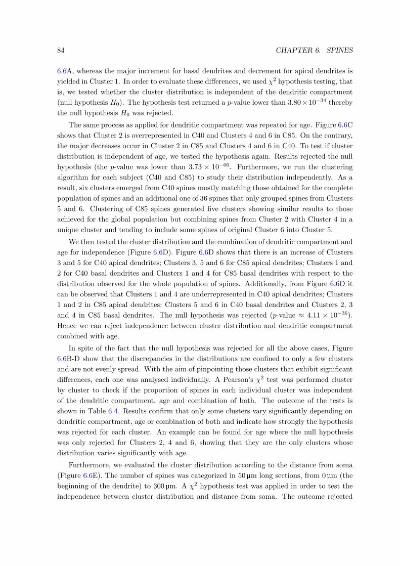
84 CHAPTER 6. SPINES
6.6A, whereas the major increment for basal dendrites and decrement for apical dendrites is
yielded in Cluster 1. In order to evaluate these differences, we used χ2 hypothesis testing, that
is, we tested whether the cluster distribution is independent of the dendritic compartment
(null hypothesis H0). The hypothesis test returned a p-value lower than 3.80×10⁻³⁴ thereby
the null hypothesis H0 was rejected.
The same process as applied for dendritic compartment was repeated for age. Figure 6.6C
shows that Cluster 2 is overrepresented in C40 and Clusters 4 and 6 in C85. On the contrary,
the major decreases occur in Cluster 2 in C85 and Clusters 4 and 6 in C40. To test if cluster
distribution is independent of age, we tested the hypothesis again. Results rejected the null
hypothesis (the p-value was lower than 3.73 × 10−06. Furthermore, we run the clustering
algorithm for each subject (C40 and C85) to study their distribution independently. As a
result, six clusters emerged from C40 spines mostly matching those obtained for the complete
population of spines and an additional one of 36 spines that only grouped spines from Clusters
5 and 6. Clustering of C85 spines generated five clusters showing similar results to those
achieved for the global population but combining spines from Cluster 2 with Cluster 4 in a
unique cluster and tending to include some spines of original Cluster 6 into Cluster 5.
We then tested the cluster distribution and the combination of dendritic compartment and
age for independence (Figure 6.6D). Figure 6.6D shows that there is an increase of Clusters
3 and 5 for C40 apical dendrites; Clusters 3, 5 and 6 for C85 apical dendrites; Clusters 1 and
2 for C40 basal dendrites and Clusters 1 and 4 for C85 basal dendrites with respect to the
distribution observed for the whole population of spines. Additionally, from Figure 6.6D it
can be observed that Clusters 1 and 4 are underrepresented in C40 apical dendrites; Clusters
1 and 2 in C85 apical dendrites; Clusters 5 and 6 in C40 basal dendrites and Clusters 2, 3
and 4 in C85 basal dendrites. The null hypothesis was rejected (p-value ≈ 4.11 × 10−36).
Hence we can reject independence between cluster distribution and dendritic compartment
combined with age.
In spite of the fact that the null hypothesis was rejected for all the above cases, Figure
6.6B-D show that the discrepancies in the distributions are confined to only a few clusters
and are not evenly spread. With the aim of pinpointing those clusters that exhibit significant
differences, each one was analysed individually. A Pearson’s χ2 test was performed cluster
by cluster to check if the proportion of spines in each individual cluster was independent
of the dendritic compartment, age and combination of both. The outcome of the tests is
shown in Table 6.4. Results confirm that only some clusters vary significantly depending on
dendritic compartment, age or combination of both and indicate how strongly the hypothesis
was rejected for each cluster. An example can be found for age where the null hypothesis
was only rejected for Clusters 2, 4 and 6, showing that they are the only clusters whose
distribution varies significantly with age.
Furthermore, we evaluated the cluster distribution according to the distance from soma
(Figure 6.6E). The number of spines was categorized in 50 µm long sections, from 0 µm (the
beginning of the dendrite) to 300 µm. A χ2 hypothesis test was applied in order to test the
independence between cluster distribution and distance from soma. The outcome rejected
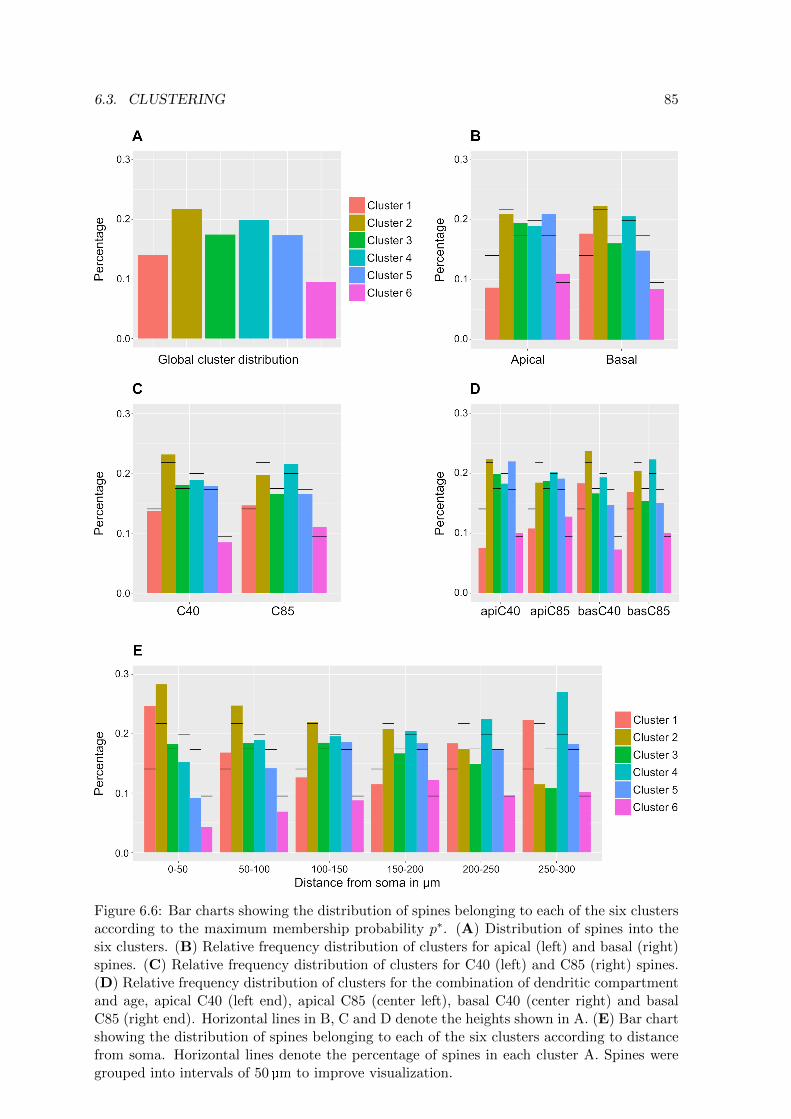
6.3. CLUSTERING 85
Figure 6.6: Bar charts showing the distribution of spines belonging to each of the six clustersaccording to the maximum membership probability p∗. (A) Distribution of spines into thesix clusters. (B) Relative frequency distribution of clusters for apical (left) and basal (right)spines. (C) Relative frequency distribution of clusters for C40 (left) and C85 (right) spines.(D) Relative frequency distribution of clusters for the combination of dendritic compartmentand age, apical C40 (left end), apical C85 (center left), basal C40 (center right) and basalC85 (right end). Horizontal lines in B, C and D denote the heights shown in A. (E) Bar chartshowing the distribution of spines belonging to each of the six clusters according to distancefrom soma. Horizontal lines denote the percentage of spines in each cluster A. Spines weregrouped into intervals of 50 µm to improve visualization.
86 CHAPTER 6. SPINES
Table 6.4: Results for Pearson’s χ2 test checking if the distribution of each cluster is inde-pendent of its dendritic compartment, age and combination of both. The * symbol denotesthat the resulting p-value is lower than 0.05 and the null hypothesis is rejected, ** denotesp-value < 0.001 and *** denotes p-value < 0.0001.
Cluster 1 Cluster 2 Cluster 3 Cluster 4 Cluster 5 Cluster 6
Dendritic compartment *** ** *** **Age * * **
Combination *** * * * *** ***
Table 6.5: Number of dendritic spines as a function of their distance from the soma
0-50 50-100 100-150 150-200 200-250 250-300
Number of spines 310 1107 2727 2407 508 148
the null hypothesis H0 (p-value ≈ 8.00 × 10⁻²³). The number of spines assigned to each
section is specified in Table 6.5. Briefly, Figure 6.6E shows that there is a predominance of
Clusters 1 and 2 at proximal distances (0-50 µm) whereas Clusters 1 and 4 show a higher
percentage than expected at longer distances.
6.3.3 Directional-linear clustering of dendritic spines
As an illustrate example, we present an alternative clustering of 500 dendritic spines randomly
subsampled from the complete dataset of 7916 dendritic spines based on the hybrid Gaussian-
von Mises mixture model. We limit the number of spines because of publishing reasons during
the development of the thesis.
Meshes had to be previously transformed into data characterising the morphology of the
spines. This task was addressed using the multiresolutional Reeb graph (MRG) [Hilaga et al.,
2001; Tangelder and Veltkamp, 2008] which partitions a triangular mesh into seven regions
(see Section 6.2.2). For each region, we measured morphological characteristics, i.e, length,
growth direction, eccentricity, flatness and size of the region (see Figure 6.3).
Since this experiment serves merely to illustrate an application of the proposed model
and does not represent any valid neuroscientific result, we then jittered data with Gaussian
and von Mises noise of zero mean. We ran the general hybrid model several times, modifying
the number of clusters from two to ten. As a result, we managed to maximize the BIC
score and Akaike information criterion score for three clusters and seven clusters respectively.
We analysed exclusively the results provided by BIC score because its number of clusters is
closest to the number of categories in the traditional classification.
To characterise clusters and compare them with the classification in [Peters and Kaiserman-
Abramof, 1970], we performed a Welch t-test [Welch, 1947] for linear variables and a Watson-
Williams test [Watson and Williams, 1956] for directional variables. We observed that almost
all linear variables are significantly different between cluster 2 and the other two clusters.
However, cluster 1 and cluster 3 only differ in so far as cluster 3 has a small neck at the

6.4. SIMULATION 87
base of the spine. We checked which cluster takes the maximum and minimum value for each
measured feature to characterise the spine.
Thus, cluster 1 presents the shortest and flattest regions. Besides, all the regions are of
the same size. This description fits the stubby class. Cluster 2 shows the longest and most
elongated regions. Additionally, the size of the regions increases from the base to the top
and the growth of the regions is less straight. Hence, this cluster groups filopodium and thin
classes. Cluster 3 has short regions and a small base. This cluster grows backwards (in a3π2 direction) while the other two clusters grow to the left (in a π direction). It apparently
matches the mushroom class.
Figure 6.7: Examples of spines for each cluster discovered by the hybrid Gaussian-von Misesmixture model. The spine representing cluster 1 is shaded green, the spine representingcluster 2 is shaded blue and the spine representing cluster 3 is shaded red.
The SEM algorithm also provides some interesting information about the dependencies
represented by the graph topology. For example, we find that the length of the next region
depends on the length of the previous regions. Also the size of the regions is related to the
size of previous regions. We also observe connections between the eccentricity of the region
and its length. These dependencies may be relevant for the electrophysiological behaviour of
the spine.
6.4 Simulation
The simulation process aimed at achieving accurate 3D representations of spines generated
by the computer. This process is divided into two main phases. First, we sampled new
instances from the mixture model. In this case we focus on the Gaussian mixture model that
discovered six groups of dendritic spines although it can be adapted to any mixture model
88 CHAPTER 6. SPINES
based on other probability distribution as the hybrid Gaussian-von Mises. As a result of
sampling, we got a dataset where each instance consisted of a vector with 54 feature values
defined by a multiresolution Reeb graph. This set of features unambiguously specifies the
position and orientation of ellipses that define the skeleton of a simulated spine. Second, we
generated a 3D representation for each instance. From the set of features of a sampled spine,
we built a skeleton composed of the ellipses establishing the beginning and end of regions
(Figure 6.8A). Because all the ellipses had the same number of points, each pair of consecutive
ellipses was easily triangulated to obtain a closed mesh (Figure 6.8B-C). Although this mesh
is a 3D spine, simulated spines have an artificial appearance because the regions delimited
by the ellipses are clearly distinguishable between them (Figure 6.8C). We improved this
result by smoothing the surface with the Loop’s subdivision algorithm [Loop, 1987]. Thus,
we obtained a more accurate 3D representation of the spine (Figure 6.8D). Examples of
simulations of each cluster can be found in Figure 6.8E. R code, model and dataset to perform
clustering and simulation of dendritic spines can be downloaded from https://github.com/
sergioluengosanchez/spineSimulation.
To be useful for future research, simulated spines must be geometrically equivalent to
real spines. Thus, simulated and real must be indistinguishable. To test for equivalence,
we state a supervised classification problem within each cluster, where the possible labels
are “simulated” vs. “real”. Hence, if both groups were indistinguishable, a classifier would
perform badly, having a classification accuracy of around 50%. To objectively validate the
realism of the simulated spines we used the RIPPER algorithm. First, for each cluster,
we sampled from the probability distribution of each cluster the same number of simulated
spines as real spines are. Second, we combined these with real spines to generate a dataset
for each cluster. Third, we applied the RIPPER algorithm with ten-fold cross-validation
[Kohavi, 1995] over the datasets to discriminate between real and simulated spines. This
process yields classifier accuracy, which can be regarded as the degree of realism. As a result
we obtained that both groups of spines are almost indistinguishable (accuracy being around
60%), with the exception of cluster 1 (80%), where the size of simulated spines is usually
somewhat larger than real spines.
6.5 Conclusions
In this chapter we used over 7,000 complete manual 3D reconstructions of dendritic spines of
human cortical pyramidal neurons to perform clustering based on their morphology. Because
the spines present artifacts due to the diffraction limits of the light, we proposed a protocol
to accurately represent the morphology of the spine. Then, model-based clustering methods
used in this study uncovered six different classes of human spines in terms of a particular set
of features according to the BIC value (see Figure 6.4A). Compared to the previous clustering
of spines [Bokota et al., 2016; Ghani et al., 2016], our proposal describes more accurately the
morphology of the spines as we consider 3D reconstructions instead of 2D; and a univocal set
of features that includes measurements of major morphological aspects like length, width or

6.5. CONCLUSIONS 89
Figure 6.8: Simulation of 3D dendritic spines. (A) Skeleton built from the set of featurescomputed according to the multiresolution Reeb graph. (B) Generation of the surface be-tween two ellipses through the triangulation of the region. (C) 3D representation of a spine.Once all the regions of the spine have been triangulated, the spine is a closed mesh used tovisualize an artificial spine. (D) Improved spine representation. Loop’s subdivision algorithmyields a smoother and more realistic version of the artificial spine. (E) Examples of simulatedspines for each cluster.

90 CHAPTER 6. SPINES
size of the spine, but also other aspects such as curvature. Additionally, our model ascribed
most of the spines to a cluster with a high cluster membership probability, but some dendritic
spines could not be clearly assigned to a group showing transition morphologies, which is
consistent with the results reported by both works.
Interestingly, we observed that there are particular clusters of spines that are proportion-
ally highly represented in a particular dendritic compartment/age combination. Specifically,
basal dendrites contained a higher proportion of the small Cluster 1 spines (Figure 6.4B),
whereas apical dendrites contained a higher proportion of the medium/large Clusters 3, 5 and
6 spines. These differences would imply that their functional properties should be expected to
be different in the two dendritic compartments [Araya, 2014]. Regarding individuals, Cluster
2 spines accounted for a higher percentage in the younger individual, whereas Clusters 4 and
6 of bigger spines had higher values than the mean percentage in the older individual. Since
small spines have been reported to be preferential sites for long-term potentiation induction
and large spines might represent physical traces of long-term memory [Kasai et al., 2010;
Matsuzaki et al., 2004b], the results suggest that the younger individual has a higher poten-
tial for plasticity than the aged case. The dendritic compartment/age combination results
also agreed with the previously reported study [Benavides-Piccione et al., 2012] that found
that apical dendrites have longer spines than basal dendrites, and younger basal dendrites are
significantly smaller than aged basal dendrites. For example, small and short spines of aged
basal dendrites and long spines of apical dendrites were lost. Regarding the distance from
soma, there is a higher predominance of the small Clusters 1 and 2 spines than expected at
proximal distances (0-50 µm) and the small Cluster 1 spines at distal distances. Also, distal
distances showed a higher percentage of the medium-sized Cluster 4 spines than expected.
Since variations in spine geometry reflect different functional properties of the spine, this
particular distribution of spines might be related to the morphofunctional compartmental-
ization of the dendrites along the length of the dendritic pyramidal neurons. For example,
it has been reported that different domains of the basal dendritic arbors of pyramidal cells
have different properties with respect to afferent connectivity, plasticity and integration rules
[Benavides-Piccione et al., 2012; Gelfo et al., 2009; Gordon et al., 2006; Hausser and Mel,
2003; Markram et al., 1997; Petreanu et al., 2009]. Thus, these results may be a reflection of
a functional dendritic organization based on spine geometry.
Using the technique of model-based clustering described in this study, we were able to
simulate accurate spines from human pyramidal neurons. This is important for three main
reasons. First, it is not necessary to store large volumes of data because all the information is
summarised in the mathematical model. Second, spines are known to be dynamic structures
(see Berry and Nedivi [2017] for a recent review), and changes in spine morphology have
important functional implications potentially affecting not only the storage and integration of
excitatory inputs in pyramidal neurons but also mediating evoked and experience-dependent
synaptic plasticity. This, in turn, has major repercussions on cognition and memory [Araya
et al., 2014; Kasai et al., 2010; Holtmaat and Svoboda, 2009; Segal, 2017; Tønnesen et al.,
2014; Van Harreveld and Fifkova, 1975]. Thus, it is necessary to link the structural data
6.5. CONCLUSIONS 91
with theoretical studies and physiological data on spines in order to interpret and make the
geometrical data on spines more meaningful. Functional modeling of spines is commonly
carried out according to their values of surface area, spine maximum diameter, spine neck
diameter, spine length, and spine neck length. Since each cluster contains a spine population
with a range of morphological features, it is necessary to model all of these morphological
variations within each cluster in order to compare the possible functional differences between
the clusters found in the present study. Third, one of the major goals in neuroscience is
to simulate human brain neuronal circuitry based on data-driven models because ethical
limitations prevent all of the necessary datasets from being acquired directly from human
brains. Therefore, the implementation of this mathematical model of human pyramidal spines
in current models of pyramidal neurons is a potentially useful tool for translating neuronal
circuitry components from experimental animals to human brain circuits. The simulation
of the spines in this study represents a mathematical model that could be implemented in
pyramidal cell models [Eyal et al., 2016] in order to present the data in a form that can be
used to reason, make predictions and suggest new hypotheses of the functional organization
of the pyramidal neurons.

92 CHAPTER 6. SPINES
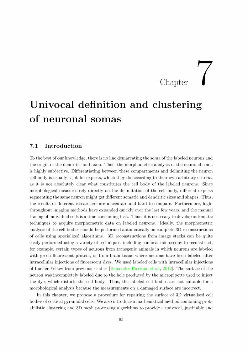
Chapter 7Univocal definition and clustering
of neuronal somas
7.1 Introduction
To the best of our knowledge, there is no line demarcating the soma of the labeled neurons and
the origin of the dendrites and axon. Thus, the morphometric analysis of the neuronal soma
is highly subjective. Differentiating between these compartments and delimiting the neuron
cell body is usually a job for experts, which they do according to their own arbitrary criteria,
as it is not absolutely clear what constitutes the cell body of the labeled neurons. Since
morphological measures rely directly on the delimitation of the cell body, different experts
segmenting the same neuron might get different somatic and dendritic sizes and shapes. Thus,
the results of different researchers are inaccurate and hard to compare. Furthermore, high-
throughput imaging methods have expanded quickly over the last few years, and the manual
tracing of individual cells is a time-consuming task. Thus, it is necessary to develop automatic
techniques to acquire morphometric data on labeled neurons. Ideally, the morphometric
analysis of the cell bodies should be performed automatically on complete 3D reconstructions
of cells using specialized algorithms. 3D reconstructions from image stacks can be quite
easily performed using a variety of techniques, including confocal microscopy to reconstruct,
for example, certain types of neurons from transgenic animals in which neurons are labeled
with green fluorescent protein, or from brain tissue where neurons have been labeled after
intracellular injections of fluorescent dyes. We used labeled cells with intracellular injections
of Lucifer Yellow from previous studies [Benavides-Piccione et al., 2012]. The surface of the
neuron was incompletely labeled due to the hole produced by the micropipette used to inject
the dye, which distorts the cell body. Thus, the labeled cell bodies are not suitable for a
morphological analysis because the measurements on a damaged surface are incorrect.
In this chapter, we propose a procedure for repairing the surface of 3D virtualised cell
bodies of cortical pyramidal cells. We also introduce a mathematical method combining prob-
abilistic clustering and 3D mesh processing algorithms to provide a univocal, justifiable and
93

94 CHAPTER 7. SOMA
objective characterisation of how a soma can be defined. The labeled cells were reconstructed
in 3D and were processed mathematically. Additionally, neural somas were characterised ac-
cording to their multiresolutional Reeb graph representations, which provide a geometrical
description of their morphology based on a combination of both linear and directional vari-
ables. Based on this representation of the soma, we performed model-based clustering using
the EMS mixture model (Section 5.4) and the SEM algorithm (Section 2.5), and analysed
the morphology of the resulting groups and the similarity between them. We describe the
process of simulating 3D virtual somas from the probabilistic model learned by the clustering
algorithm and provide some examples.
The content of this chapter has been partially published as Luengo-Sanchez et al. [2015]
and Luengo-Sanchez et al. [2019].
Chapter outline
In Section 7.2, we propose a procedure for repairing and segmenting the 3D reconstructions
of the cell bodies. We provide empirical results about the accuracy of our method. Addition-
ally, we use the multiresolutional Reeb graph representation to univocally characterise the
morphology of the neural soma. Section 7.3 presents the results of clustering the somas and
highlights the main characteristics of each cluster using the rule-based algorithm RIPPER.
In Section 7.4 we show the procedure for soma simulation and some simulated somas. Section
7.5 includes the conclusions.
7.2 Preprocessing
Neurons were intracellularly injected with Lucifer Yellow (LY) in layer III of the human
cingulate (25 somas), temporal (16 somas) and frontal (18 somas) cortex from a 40-years-
old human male. Somata were reconstructed in 3D using Imaris software 6.4.0 yielding,
by thresholding, a solid surface that matched the contour of the neuron. The generated
surface, called triangular mesh, was composed of two basic elements, vertices which defined
3D Cartesian points and faces that denoted the edges between vertices. Each face was a set
of three edges connecting vertices forming a triangle of the triangular mesh.
7.2.1 Repairing the soma
Soma surfaces frequently showed faults like holes or cavities produced by the intracellular
injection procedure (Figure 7.1A). MeshLab software [Cignoni et al., 2008] was used for the
purposes of both repair and segmentation by means of automatic scripts of MeshLab.
The faults on the surface were regarded as noise which should be removed. An approxi-
mation of the original shape of the soma was then computed to achieve a single closed mesh.
We called this process “repairing the soma” (Figure 7.1B-D). The first step in the repair pro-
cess consisted of distinguishing between the vertices on the surface and the vertices forming
holes, cavities or placed inside the neuron.

7.2. PREPROCESSING 95
Figure 7.1: Repair and segmentation process of neural somas. (A) Initial state of fourrepresentative pyramidal cells. (B) Neuron exposure to ambient lightning. (C) Neuron aftervertices forming holes and cavities or positioned inside the mesh have been discarded. (D)Neuron after mesh closing. (E) Vertices of the mesh colored according to shape diameterfunction to segment soma and dendrites. (F) Neuron after the basal dendrites have beenremoved. (G) Final result.
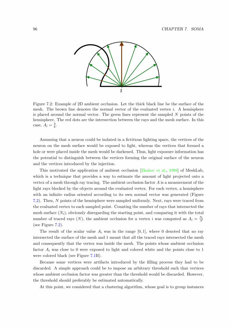
96 CHAPTER 7. SOMA
Figure 7.2: Example of 2D ambient occlusion. Let the thick black line be the surface of themesh. The brown line denotes the normal vector of the evaluated vertex i. A hemisphereis placed around the normal vector. The green lines represent the sampled N points of thehemisphere. The red dots are the intersection between the rays and the mesh surface. In thiscase, Ai = 3
8 .
Assuming that a neuron could be isolated in a fictitious lighting space, the vertices of the
neuron on the mesh surface would be exposed to light, whereas the vertices that formed a
hole or were placed inside the mesh would be darkened. Thus, light exposure information has
the potential to distinguish between the vertices forming the original surface of the neuron
and the vertices introduced by the injection.
This motivated the application of ambient occlusion [Zhukov et al., 1998] of MeshLab,
which is a technique that provides a way to estimate the amount of light projected onto a
vertex of a mesh through ray tracing. The ambient occlusion factor A is a measurement of the
light rays blocked by the objects around the evaluated vertex. For each vertex, a hemisphere
with an infinite radius oriented according to its own normal vector was generated (Figure
7.2). Then, N points of the hemisphere were sampled uniformly. Next, rays were traced from
the evaluated vertex to each sampled point. Counting the number of rays that intersected the
mesh surface (Ni), obviously disregarding the starting point, and comparing it with the total
number of traced rays (N), the ambient occlusion for a vertex i was computed as Ai = NiN
(see Figure 7.2).
The result of the scalar value Ai was in the range [0, 1], where 0 denoted that no ray
intersected the surface of the mesh and 1 meant that all the traced rays intersected the mesh
and consequently that the vertex was inside the mesh. The points whose ambient occlusion
factor Ai was close to 0 were exposed to light and colored white and the points close to 1
were colored black (see Figure 7.1B).
Because some vertices were artifacts introduced by the filling process they had to be
discarded. A simple approach could be to impose an arbitrary threshold such that vertices
whose ambient occlusion factor was greater than the threshold would be discarded. However,
the threshold should preferably be estimated automatically.
At this point, we considered that a clustering algorithm, whose goal is to group instances
7.2. PREPROCESSING 97
Figure 7.3: Mesh reconstruction. (A) The indicator function. (B) Gradient of the indicatorfunction. Since the indicator function is constant outside (0s) and inside (1s) the mesh, thegradient of the space there is 0. Only points on the frontier are not 0. (C) Inward-facingnormals and their vertices. (D) Surface of the mesh. Adapted from [Kazhdan et al., 2006].
of similar data in the same group, fitted the problem specifications exactly. Probabilistic
clustering based on a Gaussian mixture [McLachlan and Basford, 1988] was applied to cluster
vertices into two groups:
1. The vertices on the surface of the neuron.
2. The vertices forming holes and cavities or inside the neuron.
Probabilistic clustering returned the probability of each vertex being a member of either
cluster. The decision boundary between both clusters, i.e., the ambient occlusion factor for
which both groups were equiprobable, was the threshold. Vertices i whose Ai factor was
greater than the threshold were removed, as were their associated faces. As a consequence,
the mesh was opened as shown in Figure 7.1C. An approximation of the original surface of
the soma was computed to achieve a single closed mesh (Figure 7.1D) as explained below.
A simple way to define the closed surface of an object is by means of an indicator function
that denotes the space inside and outside the object as 1 and 0, respectively (Figure 7.3A).
Thus, as a result of computing the gradient of this function, space would be zero almost ev-
erywhere except near the surface of the object (Figure 7.3B). However, the indicator function
was unknown and only the vertices and the inward-facing normals of the mesh were provided
by Imaris and MeshLab software (Figure 7.3C). A relationship between the gradient of the
indicator function and an integral of the surface normal field was derived in [Kazhdan et al.,
2006]. The surface of the mesh was approximated from this integral relation (Figure 7.3D)
so the holes in the surface introduced in the previous step disappeared and the surface of the
soma was also slightly smoothed.
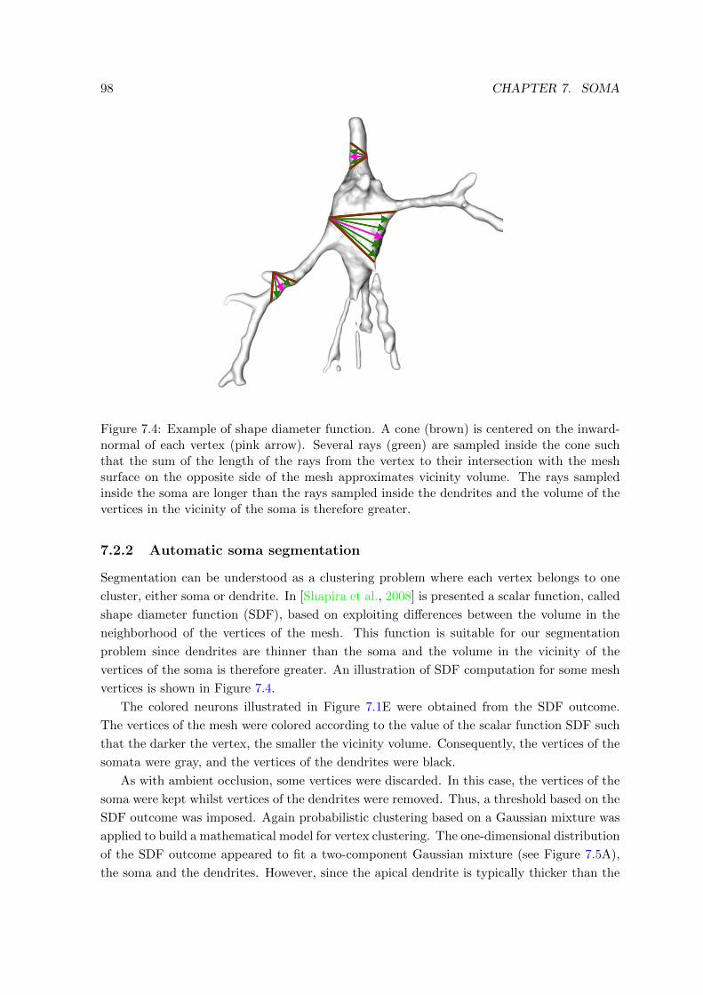
98 CHAPTER 7. SOMA
Figure 7.4: Example of shape diameter function. A cone (brown) is centered on the inward-normal of each vertex (pink arrow). Several rays (green) are sampled inside the cone suchthat the sum of the length of the rays from the vertex to their intersection with the meshsurface on the opposite side of the mesh approximates vicinity volume. The rays sampledinside the soma are longer than the rays sampled inside the dendrites and the volume of thevertices in the vicinity of the soma is therefore greater.
7.2.2 Automatic soma segmentation
Segmentation can be understood as a clustering problem where each vertex belongs to one
cluster, either soma or dendrite. In [Shapira et al., 2008] is presented a scalar function, called
shape diameter function (SDF), based on exploiting differences between the volume in the
neighborhood of the vertices of the mesh. This function is suitable for our segmentation
problem since dendrites are thinner than the soma and the volume in the vicinity of the
vertices of the soma is therefore greater. An illustration of SDF computation for some mesh
vertices is shown in Figure 7.4.
The colored neurons illustrated in Figure 7.1E were obtained from the SDF outcome.
The vertices of the mesh were colored according to the value of the scalar function SDF such
that the darker the vertex, the smaller the vicinity volume. Consequently, the vertices of the
somata were gray, and the vertices of the dendrites were black.
As with ambient occlusion, some vertices were discarded. In this case, the vertices of the
soma were kept whilst vertices of the dendrites were removed. Thus, a threshold based on the
SDF outcome was imposed. Again probabilistic clustering based on a Gaussian mixture was
applied to build a mathematical model for vertex clustering. The one-dimensional distribution
of the SDF outcome appeared to fit a two-component Gaussian mixture (see Figure 7.5A),
the soma and the dendrites. However, since the apical dendrite is typically thicker than the
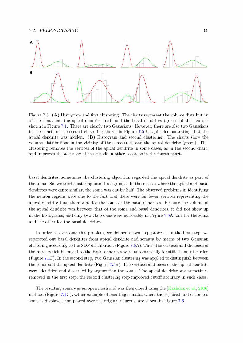
7.2. PREPROCESSING 99
Figure 7.5: (A) Histogram and first clustering. The charts represent the volume distributionof the soma and the apical dendrite (red) and the basal dendrites (green) of the neuronsshown in Figure 7.1. There are clearly two Gaussians. However, there are also two Gaussiansin the charts of the second clustering shown in Figure 7.5B, again demonstrating that theapical dendrite was hidden. (B) Histogram and second clustering. The charts show thevolume distributions in the vicinity of the soma (red) and the apical dendrite (green). Thisclustering removes the vertices of the apical dendrite in some cases, as in the second chart,and improves the accuracy of the cutoffs in other cases, as in the fourth chart.
basal dendrites, sometimes the clustering algorithm regarded the apical dendrite as part of
the soma. So, we tried clustering into three groups. In those cases where the apical and basal
dendrites were quite similar, the soma was cut by half. The observed problems in identifying
the neuron regions were due to the fact that there were far fewer vertices representing the
apical dendrite than there were for the soma or the basal dendrites. Because the volume of
the apical dendrite was between that of the soma and basal dendrites, it did not show up
in the histograms, and only two Gaussians were noticeable in Figure 7.5A, one for the soma
and the other for the basal dendrites.
In order to overcome this problem, we defined a two-step process. In the first step, we
separated out basal dendrites from apical dendrite and somata by means of two Gaussian
clustering according to the SDF distribution (Figure 7.5A). Thus, the vertices and the faces of
the mesh which belonged to the basal dendrites were automatically identified and discarded
(Figure 7.1F). In the second step, two Gaussian clustering was applied to distinguish between
the soma and the apical dendrite (Figure 7.5B). The vertices and faces of the apical dendrite
were identified and discarded by segmenting the soma. The apical dendrite was sometimes
removed in the first step; the second clustering step improved cutoff accuracy in such cases.
The resulting soma was an open mesh and was then closed using the [Kazhdan et al., 2006]
method (Figure 7.1G). Other example of resulting somata, where the repaired and extracted
soma is displayed and placed over the original neurons, are shown in Figure 7.6.

100 CHAPTER 7. SOMA
Figure 7.6: Examples of final soma result. The reconstructed neuron is colored white and itsautomatically extracted soma is denoted in red.
7.2.3 Mesh comparison
The distance between the surfaces of two triangular meshes quantifies the distortion added
by a mesh processing technique. In our case, the distance was computed to validate the
goodness of the proposed method.
The distance between two meshes is defined as the minimum distance from each point on
the surface S1 of a mesh to the surface S2 of a second mesh. As the boundaries of a mesh are
defined by its vertices, we studied the distance from vertices only. The distance ε between a
vertex p ∈ S1 and the surface S2 was computed according to [Cignoni et al., 1998] as
ε(p, S2) = minp′∈S2
d(p, p′),
where d is the Euclidean distance between p and p′ in R3. Then the root mean square error
(RMSE) was computed as follows:
RMSE(S1, S2) =
√∑p∈S1
ε(p, S2)2
|S1|,
where |S1| is the number of vertices of the surface of the mesh. RMSE is an asymmetric
measure as RMSE(S1, S2) 6= RMSE(S2, S1). A symmetric form of the RMSE was obtained
as
RMSES(S1, S2) = max{RMSE(S1, S2), RMSE(S2, S1)}.
Thus, RMSES(S1, S2) = 0 ⇐⇒ S1 = S2.
Also, it is useful to compare different mesh processing techniques. For two techniques,
one approach was based on processing M meshes with each processing method. Then the
volume of each processed mesh was calculated according to [Zhang and Chen, 2001]. Mesh
processing techniques were compared by the mean absolute quotient between volumes (MAQ).
Its outcome was an estimation of the proportional difference in volume when a method is
applied in place of the other:
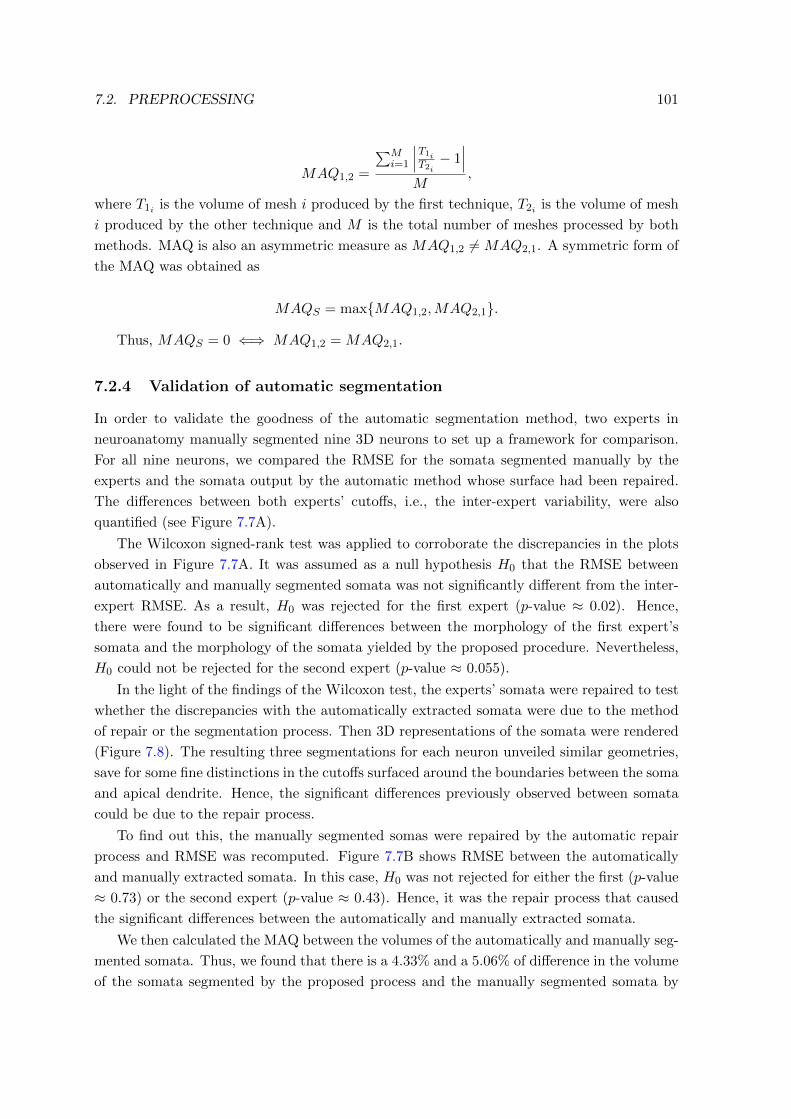
7.2. PREPROCESSING 101
MAQ1,2 =
∑Mi=1
∣∣∣T1iT2i− 1∣∣∣
M,
where T1i is the volume of mesh i produced by the first technique, T2i is the volume of mesh
i produced by the other technique and M is the total number of meshes processed by both
methods. MAQ is also an asymmetric measure as MAQ1,2 6= MAQ2,1. A symmetric form of
the MAQ was obtained as
MAQS = max{MAQ1,2,MAQ2,1}.
Thus, MAQS = 0 ⇐⇒ MAQ1,2 = MAQ2,1.
7.2.4 Validation of automatic segmentation
In order to validate the goodness of the automatic segmentation method, two experts in
neuroanatomy manually segmented nine 3D neurons to set up a framework for comparison.
For all nine neurons, we compared the RMSE for the somata segmented manually by the
experts and the somata output by the automatic method whose surface had been repaired.
The differences between both experts’ cutoffs, i.e., the inter-expert variability, were also
quantified (see Figure 7.7A).
The Wilcoxon signed-rank test was applied to corroborate the discrepancies in the plots
observed in Figure 7.7A. It was assumed as a null hypothesis H0 that the RMSE between
automatically and manually segmented somata was not significantly different from the inter-
expert RMSE. As a result, H0 was rejected for the first expert (p-value ≈ 0.02). Hence,
there were found to be significant differences between the morphology of the first expert’s
somata and the morphology of the somata yielded by the proposed procedure. Nevertheless,
H0 could not be rejected for the second expert (p-value ≈ 0.055).
In the light of the findings of the Wilcoxon test, the experts’ somata were repaired to test
whether the discrepancies with the automatically extracted somata were due to the method
of repair or the segmentation process. Then 3D representations of the somata were rendered
(Figure 7.8). The resulting three segmentations for each neuron unveiled similar geometries,
save for some fine distinctions in the cutoffs surfaced around the boundaries between the soma
and apical dendrite. Hence, the significant differences previously observed between somata
could be due to the repair process.
To find out this, the manually segmented somas were repaired by the automatic repair
process and RMSE was recomputed. Figure 7.7B shows RMSE between the automatically
and manually extracted somata. In this case, H0 was not rejected for either the first (p-value
≈ 0.73) or the second expert (p-value ≈ 0.43). Hence, it was the repair process that caused
the significant differences between the automatically and manually extracted somata.
We then calculated the MAQ between the volumes of the automatically and manually seg-
mented somata. Thus, we found that there is a 4.33% and a 5.06% of difference in the volume
of the somata segmented by the proposed process and the manually segmented somata by
102 CHAPTER 7. SOMA
Figure 7.7: RMSE before and after repairing the experts’ somata. (A) For all neuronsexcept Neuron 6, RMSE was less between experts than between the somata output by ourprocedure and by either of the experts. For several neurons, the difference was actually morethan double. (B) The differences between automatically and manually segmented somatawere not so remarkable after the repair of the experts’ somata. Note that for some neuronsRMSE was less between our procedure and the first expert than between both experts, i.e.,the proposed procedure can produce similar cutoffs to an expert
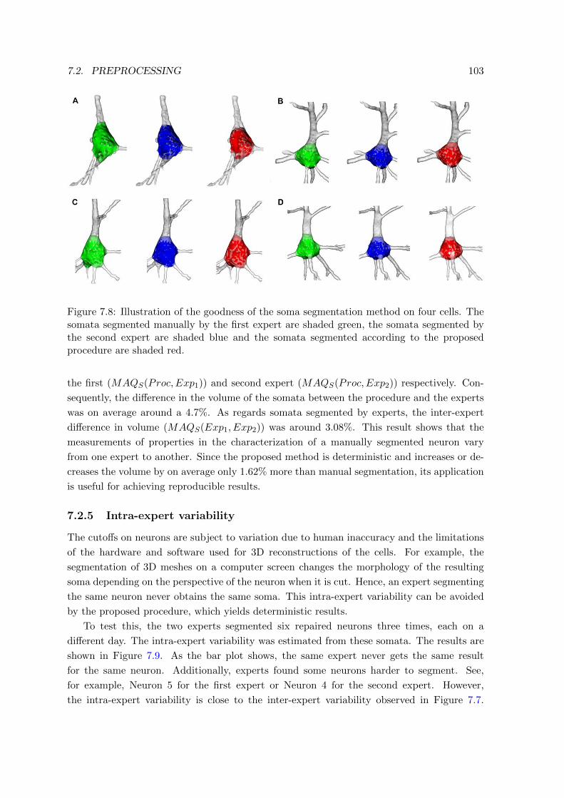
7.2. PREPROCESSING 103
Figure 7.8: Illustration of the goodness of the soma segmentation method on four cells. Thesomata segmented manually by the first expert are shaded green, the somata segmented bythe second expert are shaded blue and the somata segmented according to the proposedprocedure are shaded red.
the first (MAQS(Proc,Exp1)) and second expert (MAQS(Proc,Exp2)) respectively. Con-
sequently, the difference in the volume of the somata between the procedure and the experts
was on average around a 4.7%. As regards somata segmented by experts, the inter-expert
difference in volume (MAQS(Exp1, Exp2)) was around 3.08%. This result shows that the
measurements of properties in the characterization of a manually segmented neuron vary
from one expert to another. Since the proposed method is deterministic and increases or de-
creases the volume by on average only 1.62% more than manual segmentation, its application
is useful for achieving reproducible results.
7.2.5 Intra-expert variability
The cutoffs on neurons are subject to variation due to human inaccuracy and the limitations
of the hardware and software used for 3D reconstructions of the cells. For example, the
segmentation of 3D meshes on a computer screen changes the morphology of the resulting
soma depending on the perspective of the neuron when it is cut. Hence, an expert segmenting
the same neuron never obtains the same soma. This intra-expert variability can be avoided
by the proposed procedure, which yields deterministic results.
To test this, the two experts segmented six repaired neurons three times, each on a
different day. The intra-expert variability was estimated from these somata. The results are
shown in Figure 7.9. As the bar plot shows, the same expert never gets the same result
for the same neuron. Additionally, experts found some neurons harder to segment. See,
for example, Neuron 5 for the first expert or Neuron 4 for the second expert. However,
the intra-expert variability is close to the inter-expert variability observed in Figure 7.7.
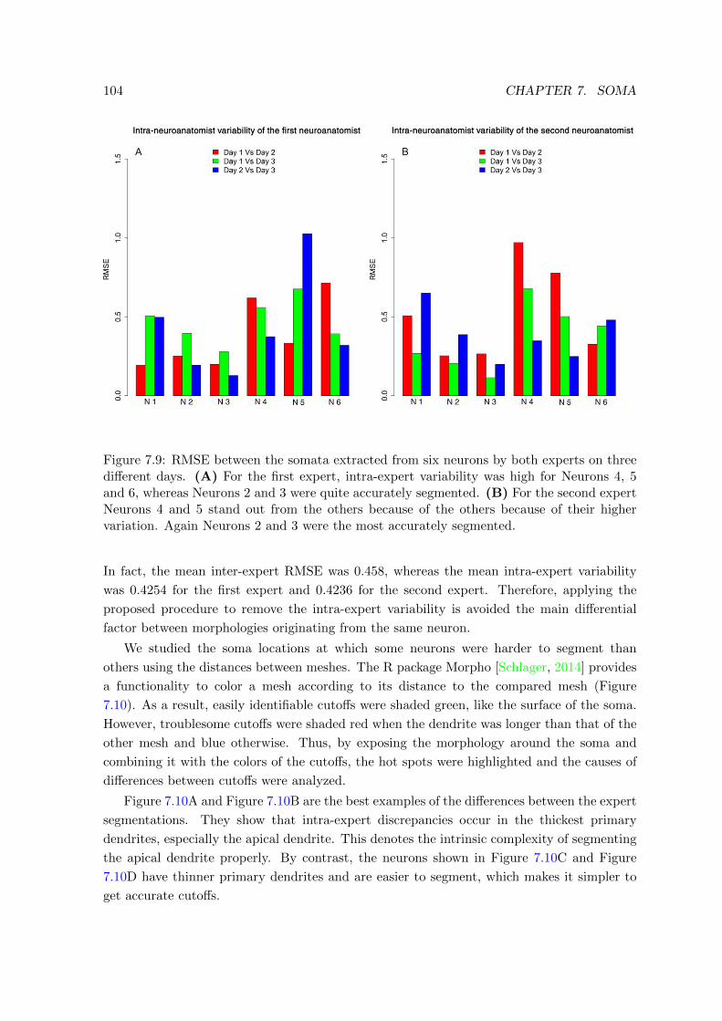
104 CHAPTER 7. SOMA
Figure 7.9: RMSE between the somata extracted from six neurons by both experts on threedifferent days. (A) For the first expert, intra-expert variability was high for Neurons 4, 5and 6, whereas Neurons 2 and 3 were quite accurately segmented. (B) For the second expertNeurons 4 and 5 stand out from the others because of the others because of their highervariation. Again Neurons 2 and 3 were the most accurately segmented.
In fact, the mean inter-expert RMSE was 0.458, whereas the mean intra-expert variability
was 0.4254 for the first expert and 0.4236 for the second expert. Therefore, applying the
proposed procedure to remove the intra-expert variability is avoided the main differential
factor between morphologies originating from the same neuron.
We studied the soma locations at which some neurons were harder to segment than
others using the distances between meshes. The R package Morpho [Schlager, 2014] provides
a functionality to color a mesh according to its distance to the compared mesh (Figure
7.10). As a result, easily identifiable cutoffs were shaded green, like the surface of the soma.
However, troublesome cutoffs were shaded red when the dendrite was longer than that of the
other mesh and blue otherwise. Thus, by exposing the morphology around the soma and
combining it with the colors of the cutoffs, the hot spots were highlighted and the causes of
differences between cutoffs were analyzed.
Figure 7.10A and Figure 7.10B are the best examples of the differences between the expert
segmentations. They show that intra-expert discrepancies occur in the thickest primary
dendrites, especially the apical dendrite. This denotes the intrinsic complexity of segmenting
the apical dendrite properly. By contrast, the neurons shown in Figure 7.10C and Figure
7.10D have thinner primary dendrites and are easier to segment, which makes it simpler to
get accurate cutoffs.
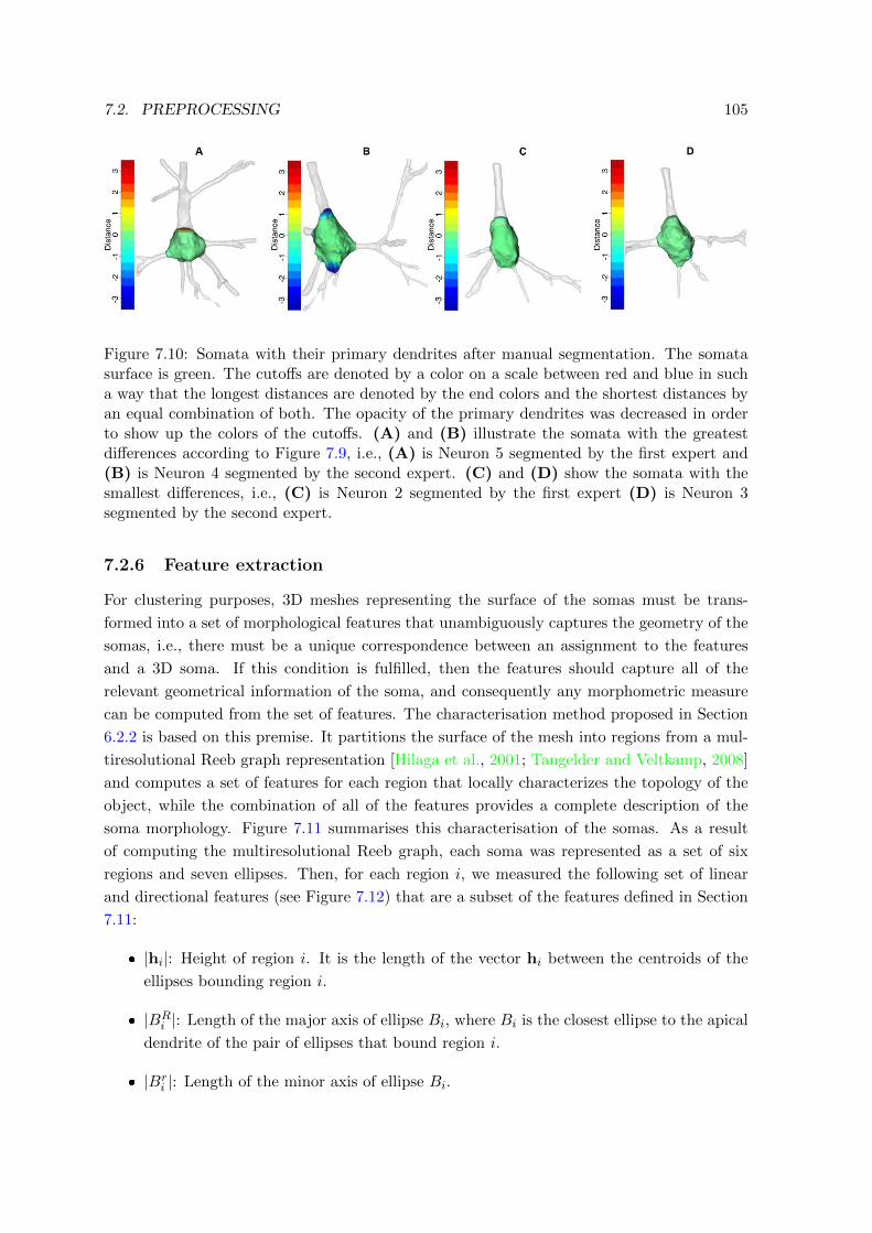
7.2. PREPROCESSING 105
Figure 7.10: Somata with their primary dendrites after manual segmentation. The somatasurface is green. The cutoffs are denoted by a color on a scale between red and blue in sucha way that the longest distances are denoted by the end colors and the shortest distances byan equal combination of both. The opacity of the primary dendrites was decreased in orderto show up the colors of the cutoffs. (A) and (B) illustrate the somata with the greatestdifferences according to Figure 7.9, i.e., (A) is Neuron 5 segmented by the first expert and(B) is Neuron 4 segmented by the second expert. (C) and (D) show the somata with thesmallest differences, i.e., (C) is Neuron 2 segmented by the first expert (D) is Neuron 3segmented by the second expert.
7.2.6 Feature extraction
For clustering purposes, 3D meshes representing the surface of the somas must be trans-
formed into a set of morphological features that unambiguously captures the geometry of the
somas, i.e., there must be a unique correspondence between an assignment to the features
and a 3D soma. If this condition is fulfilled, then the features should capture all of the
relevant geometrical information of the soma, and consequently any morphometric measure
can be computed from the set of features. The characterisation method proposed in Section
6.2.2 is based on this premise. It partitions the surface of the mesh into regions from a mul-
tiresolutional Reeb graph representation [Hilaga et al., 2001; Tangelder and Veltkamp, 2008]
and computes a set of features for each region that locally characterizes the topology of the
object, while the combination of all of the features provides a complete description of the
soma morphology. Figure 7.11 summarises this characterisation of the somas. As a result
of computing the multiresolutional Reeb graph, each soma was represented as a set of six
regions and seven ellipses. Then, for each region i, we measured the following set of linear
and directional features (see Figure 7.12) that are a subset of the features defined in Section
7.11:
� |hi|: Height of region i. It is the length of the vector hi between the centroids of the
ellipses bounding region i.
� |BRi |: Length of the major axis of ellipse Bi, where Bi is the closest ellipse to the apical
dendrite of the pair of ellipses that bound region i.
� |Bri |: Length of the minor axis of ellipse Bi.

106 CHAPTER 7. SOMA
� cos θi: Curvature of the soma at region i. Taking vector hi as the zenith of a spherical
coordinate system, vectors hi and hi+1 define a direction that can be expressed in
spherical coordinates, i.e., the azimuth angle φi and elevation angle θi. The curvature
is computed from the dot product cos θi = hi·hi+1
|hi||hi+1| . Note that, although θi is an angle,
and it is not periodical because its domain is [0, π]. In [Mardia, 1975b], it is discussed
that the suitability of modelling random angles is clearly restricted to an interval smaller
than 2π as circular variates, concluding that these angles should be treated like ordinary
linear variables. Hence, we considered θi as a linear variable.
� φi: Growing direction of region i. It is the azimuth angle computed from vectors hi
and hi+1 that, combined with θi, describes the direction of a vector hi+1 in spherical
coordinates.
� Θi: Direction of ellipse Bi. It is the polar angle or colatitude in the spherical coordinate
system defined by the perpendicular vector to ellipse Bi, assuming the centroid of the
ellipse as the origin. It is obtained from the vectorBRi|BRi |× Bri|Bri |
. It was considered as a
linear variable for the same reason as θi.
� Φi: Direction of ellipse Bi. The azimuth or azimuthal angle in the spherical coordinate
system defined by the perpendicular vector to the ellipse Bi assuming the centroid of
the ellipse as the origin. It is obtained from the vectorBRi|BRi |× Bri|Bri |
. Both Θi and Φi
together describe the direction of the perpendicular vector to Bi.
7.3 Clustering
The morphology of a soma was approximated with 43 variables, where 12 of them are di-
rectional and 31 are linear. According to this characterisation, the number of variables was
larger than the number of repaired somas. When the number of parameters to estimate is
larger than the amount of data available, the model can overfit the data, or the covariance
matrix can even become singular for some clusters. This problem gets worse in model-based
clustering, as the number of parameters of the model increases linearly with the number of
components of the mixture. Hence, we had to constrain the degrees of freedom of the model
by introducing an upper bound to the maximum number of parents for each node, as well
as the number of clusters. Another implementation detail is related to the SEM algorithm,
which guarantees the convergence to a stationary point (local optimum, global optimum or
a saddle point), which can be non-optimal in some cases. Because SEM is a determinis-
tic algorithm, the starting point dictates the convergence point. To reduce the probability
of converging to undesirable stationary points, SEM algorithm was initialised from several
random uniformly distributed starting points. We empirically set the maximum number of
parents to two for the structure learning and executed the SEM algorithm 300 times from
randomly selected starting points for two and three clusters.
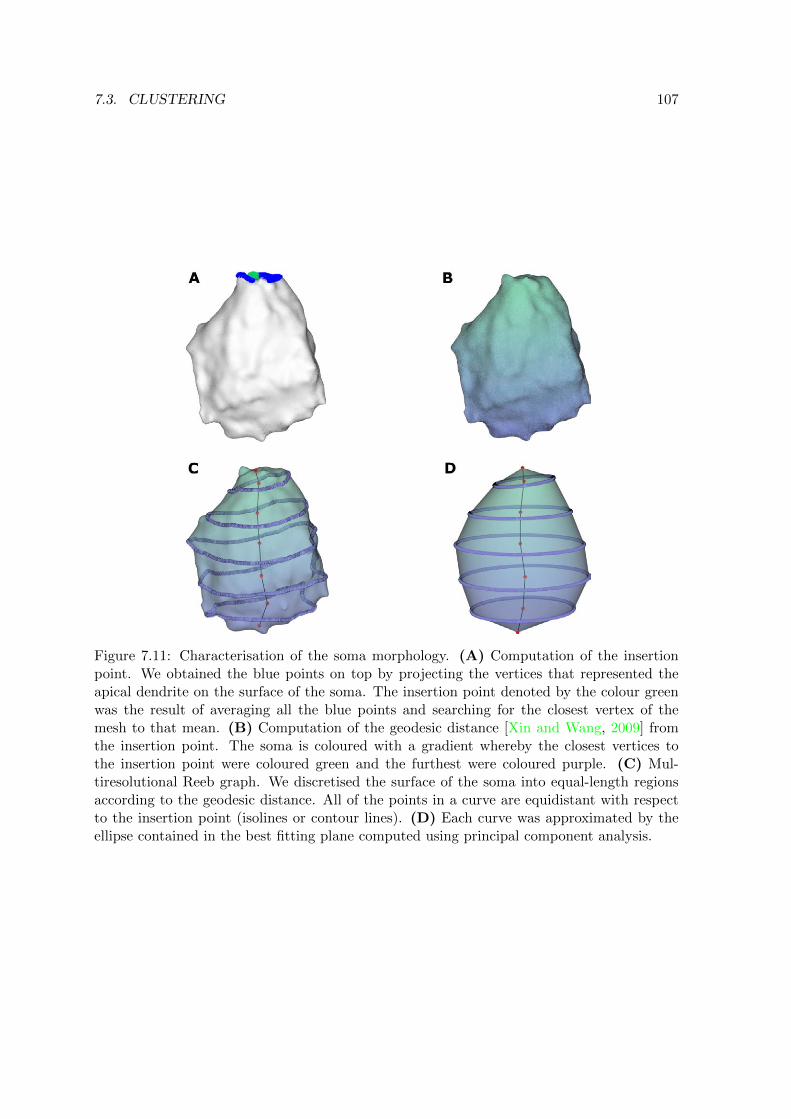
7.3. CLUSTERING 107
Figure 7.11: Characterisation of the soma morphology. (A) Computation of the insertionpoint. We obtained the blue points on top by projecting the vertices that represented theapical dendrite on the surface of the soma. The insertion point denoted by the colour greenwas the result of averaging all the blue points and searching for the closest vertex of themesh to that mean. (B) Computation of the geodesic distance [Xin and Wang, 2009] fromthe insertion point. The soma is coloured with a gradient whereby the closest vertices tothe insertion point were coloured green and the furthest were coloured purple. (C) Mul-tiresolutional Reeb graph. We discretised the surface of the soma into equal-length regionsaccording to the geodesic distance. All of the points in a curve are equidistant with respectto the insertion point (isolines or contour lines). (D) Each curve was approximated by theellipse contained in the best fitting plane computed using principal component analysis.
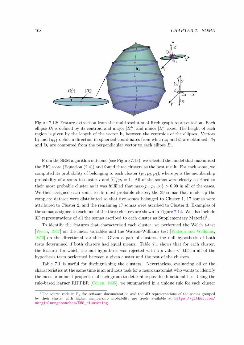
108 CHAPTER 7. SOMA
Figure 7.12: Feature extraction from the multiresolutional Reeb graph representation. Eachellipse Bi is defined by its centroid and major |BR
i | and minor |Bri | axes. The height of each
region is given by the length of the vector hi between the centroids of the ellipses. Vectorshi and hi+1 define a direction in spherical coordinates from which φi and θi are obtained. Φi
and Θi are computed from the perpendicular vector to each ellipse Bi.
From the SEM algorithm outcome (see Figure 7.13), we selected the model that maximised
the BIC score (Equation (2.4)) and found three clusters as the best result. For each soma, we
computed its probability of belonging to each cluster (p1, p2, p3), where pi is the membership
probability of a soma to cluster i and∑3
i pi = 1. All of the somas were clearly ascribed to
their most probable cluster as it was fulfilled that max{p1, p2, p3} > 0.99 in all of the cases.
We then assigned each soma to its most probable cluster; the 39 somas that made up the
complete dataset were distributed so that five somas belonged to Cluster 1, 17 somas were
attributed to Cluster 2, and the remaining 17 somas were ascribed to Cluster 3. Examples of
the somas assigned to each one of the three clusters are shown in Figure 7.14. We also include
3D representations of all the somas ascribed to each cluster as Supplementary Material1.
To identify the features that characterised each cluster, we performed the Welch t-test
[Welch, 1947] on the linear variables and the Watson-Williams test [Watson and Williams,
1956] on the directional variables. Given a pair of clusters, the null hypothesis of both
tests determined if both clusters had equal means. Table 7.1 shows that for each cluster,
the features for which the null hypothesis was rejected with a p-value < 0.05 in all of the
hypothesis tests performed between a given cluster and the rest of the clusters.
Table 7.1 is useful for distinguishing the clusters. Nevertheless, evaluating all of the
characteristics at the same time is an arduous task for a neuroanatomist who wants to identify
the most prominent properties of each group to determine possible functionalities. Using the
rule-based learner RIPPER [Cohen, 1995], we summarised in a unique rule for each cluster
1The source code in R, the software documentation and the 3D representations of the somas groupedby their cluster with higher membership probability are freely available at https://github.com/sergioluengosanchez/EMS_clustering.
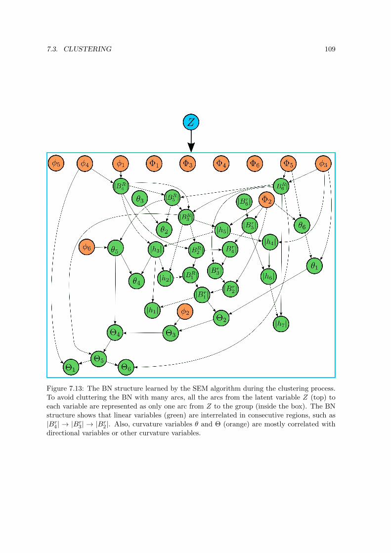
7.3. CLUSTERING 109
Figure 7.13: The BN structure learned by the SEM algorithm during the clustering process.To avoid cluttering the BN with many arcs, all the arcs from the latent variable Z (top) toeach variable are represented as only one arc from Z to the group (inside the box). The BNstructure shows that linear variables (green) are interrelated in consecutive regions, such as|Br
4| → |Br3| → |Br
2|. Also, curvature variables θ and Θ (orange) are mostly correlated withdirectional variables or other curvature variables.
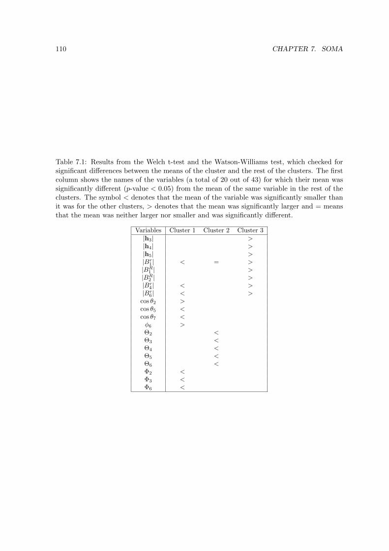
110 CHAPTER 7. SOMA
Table 7.1: Results from the Welch t-test and the Watson-Williams test, which checked forsignificant differences between the means of the cluster and the rest of the clusters. The firstcolumn shows the names of the variables (a total of 20 out of 43) for which their mean wassignificantly different (p-value < 0.05) from the mean of the same variable in the rest of theclusters. The symbol < denotes that the mean of the variable was significantly smaller thanit was for the other clusters, > denotes that the mean was significantly larger and = meansthat the mean was neither larger nor smaller and was significantly different.
Variables Cluster 1 Cluster 2 Cluster 3|h3| >|h4| >|h5| >|Br
1 | < = >|BR
1 | >|BR
2 | >|Br
4 | < >|Br
6 | < >cos θ2 >cos θ5 <cos θ7 <φ6 >Θ2 <Θ3 <Θ4 <Θ5 <Θ6 <Φ2 <Φ3 <Φ6 <
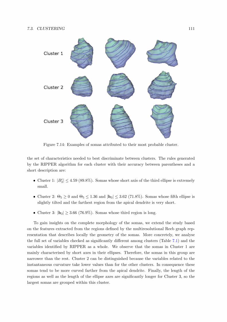
7.3. CLUSTERING 111
Figure 7.14: Examples of somas attributed to their most probable cluster.
the set of characteristics needed to best discriminate between clusters. The rules generated
by the RIPPER algorithm for each cluster with their accuracy between parentheses and a
short description are:
� Cluster 1: |Br3| ≤ 4.59 (89.8%). Somas whose short axis of the third ellipse is extremely
small.
� Cluster 2: Θ5 ≥ 0 and Θ5 ≤ 1.36 and |h3| ≤ 3.62 (71.8%). Somas whose fifth ellipse is
slightly tilted and the farthest region from the apical dendrite is very short.
� Cluster 3: |h3| ≥ 3.66 (76.9%). Somas whose third region is long.
To gain insights on the complete morphology of the somas, we extend the study based
on the features extracted from the regions defined by the multiresolutional Reeb graph rep-
resentation that describes locally the geometry of the somas. More concretely, we analyse
the full set of variables checked as significantly different among clusters (Table 7.1) and the
variables identified by RIPPER as a whole. We observe that the somas in Cluster 1 are
mainly characterised by short axes in their ellipses. Therefore, the somas in this group are
narrower than the rest. Cluster 2 can be distinguished because the variables related to the
instantaneous curvature take lower values than for the other clusters. In consequence these
somas tend to be more curved farther from the apical dendrite. Finally, the length of the
regions as well as the length of the ellipse axes are significantly longer for Cluster 3, so the
largest somas are grouped within this cluster.

112 CHAPTER 7. SOMA
From a neuroanatomical point of view, neurons with similar morphologies perform anal-
ogous brain functions. Therefore, it is interesting to find out which clusters of morphologies
were more similar to each other. For this purpose, we computed the KL divergence between
the three subtypes of pyramidal somas uncovered by our clustering approach. Thus, we ob-
tained that the most similar clusters were Cluster 1 and Cluster 3 with a KL divergence of
869.4. Cluster 2 brought together the most different morphologies, as its KL divergences with
respect to Cluster 1 and Cluster 3 were 2,078.3 and 1,629.0, respectively.
7.4 Simulation
One of the main challenges faced by neuroscience is the simulation of the human brain
circuitry based on mathematical models (see Section 4.1). Given that ethical limitations
prevent acquisition of the data directly from human brains, statistical models present an
opportunity to reason, make predictions and suggest new hypotheses. The generative model
implemented in this study allowed us to simulate virtual somas following the same two-step
process described for dendritic spines in Section 6.4. First, new datasets were sampled from
the joint p.d.f. represented by the learned BN. Then, for each instance of the new dataset, the
3D representation of the soma was generated. Note that the univocal correspondence between
an assignment to the variables and the geometry of the soma enabled the 3D reconstruction.
The procedure to obtain a virtual soma and some examples of virtual somas simulated from
each cluster are shown in Figure 7.15.
7.5 Conclusions
In this study we provide a mathematical definition of the neuronal soma and an automatic
segmentation method to delimit the neuronal soma of pyramidal cells. Since there are no
benchmarks with which to compare the proposed procedure, we validated the goodness of
this automatic segmentation method against the manual segmentation performed by experts
in neuroanatomy in order to set up a framework for comparison.
The results have demonstrated the importance of the repair process. Significant differ-
ences were found between the morphology of the cell bodies with and without a reconstructed
surface. However, after repairing the surface of the somata, there were no significant differ-
ences between automatically and manually segmented somata, i.e., the proposed procedure
segments the neurons more or less as an expert would. It also provides univocal, justifiable
and objective cutoffs. The cutoffs on neurons are subject to variation due to human inaccu-
racy and the limitations of the software used for 3D reconstructions of the cells. Furthermore,
manual tracing of individual cells is a time-consuming task. It is, therefore, important to
develop automated methods for the morphological analysis of large numbers of neurons to
enable high-throughput research.
We think that the mathematical definition of the soma of pyramidal cells is an important
step not only towards establishing and maintaining effective communication and data sharing

7.5. CONCLUSIONS 113
Figure 7.15: Simulation of virtual somas. (A) The skeleton is created. First, the insertionpoint (green) is placed at the origin of the coordinates. For each ellipse, compute the co-ordinates of its centroid from the centroid of the previous ellipse using the height |hi|, thecurvature cos θi and the growing direction φi of region i. (B) An ellipse for each centroid isgenerated. Given the centroid at the bottom of region i, 360 points are sampled from ellipseBi defined by the length of its axes, |BR
i | and |Bri |, and its inclination given by Θi and Φi.
(C) Finally, consecutive ellipses are triangulated to obtain a closed mesh. (D) Examples ofvirtual somas simulated from each cluster.
114 CHAPTER 7. SOMA
between different laboratories, but also for better characterising these cells. For example, it is
well known that these cells are heterogeneous with regard to soma size and shape and different
subpopulations of pyramidal cells have different size [Hendry and Jones, 1983]. However, there
are no accurate morphometric data, and the data variations between different laboratories
may simply reflect the discrepancy regarding the delimitation of the cell body. We thin that
an undertaking by different laboratories to use the same methodology to define the soma
would have a great impact. The reason is that this information is relevant not only for better
characterizing the morphology of these cells in different cortical areas and species but also
for annotating and exchanging relevant information for modeling the activity of these cells.
For example, the method that we propose will help to generate detailed functional models
requiring knowledge of number of density of axo-somatic synapses, or of when quantitative
data about molecules playing a key role in the physiology of these cells are critical, for
example, to the density of different voltage-gated ion channels and receptors on the somatic
membrane surface area.
Previous studies have reported variations in the size of pyramidal neurons, but these
studies are based on arbitrary soma measurements, impeding comparisons between different
laboratories or the performance of other correlational studies, such as the possible relationship
between the size of the soma and the number of branches, nodes, etc., of the dendritic tree.
Thus, this study is an excellent means for further characterizing pyramidal neurons in order
to objectively compare the morphometry of the somata of these neurons in different cortical
areas and species and try to find possible rules governing the geometric design of pyramidal
cells.
We applied our EMS finite mixture model to the neuroscientific problem of clustering neu-
ral somas by their morphology. The characterisation of the somas according to the adapted
multiresolution Reeb graph representation enabled 3D simulation of virtual somas from the
three groups found by the SEM algorithm. We also identified the most prominent charac-
teristics of each cluster by means of hypothesis tests and the RIPPER algorithm which can
provide the neuroanatomist a deeper insight about the relation between morphology and
functionality of the soma.

Part V
CONCLUSIONS AND FUTURE
WORK
115

Chapter 8Conclusions and future work
In this chapter we highlight the most important contributions and describe future research
work. The chapter also includes a list enumerating the publications and submissions product
of this research.
8.1 Summary of contributions
The contributions have been divided into two parts:
� Part III includes our contribution to directional statistics and data clustering. In Chap-
ter 5 we propose a set of finite mixture models for clustering multivariate directional
and directional-linear data according to closed-form expressions, avoiding numerical
optimisation methods that can be extremely computational expensive in combination
with the EM algorithm. Using the SEM algorithm we are able to learn the conditional
dependencies among variables encoded by the structure of the BN while we discover
the clusters. This provides several advantages such as the interpretability of the model,
the control over the complexity of the model and the possibility to manually include
constraints in the relationships between variables. We also present the multivariate
extension of the Mardia-Sutton distribution which allows us to relax the independence
constraints among directional and linear variables of previous directional-linear mod-
els applied in clustering. Additionally we derive the closed-form expressions for the
Kullback-Leibler divergence and Bhattacharyya distance which are similarity measures
between distributions that can be useful to evaluate the quality of the clusters.
� Part IV presents our work on clustering and simulation of 3D dendritic spines and
neuronal somas. Chapter 6 details the geometrical clustering results from over 7,000
complete manual 3D reconstructions of human cortical pyramidal neuron spines. First,
we propose a repairing protocol to accurately represent the morphology of the spines
which presented artifacts due to the diffraction limits of the light. Then, we compute a
set of features that summarise the morphology of the spine. These characterisation un-
ambiguously captures the geometry of the spines, i.e., there is a unique correspondence
117

118 CHAPTER 8. CONCLUSIONS AND FUTURE WORK
between an assignment to the features and a 3D representation of the spine. Thus, the
features capture all the relevant geometrical information and consequently any mor-
phometric measure can be computed from these set of features. From this dataset we
learn a Gaussian mixture model that uncovered six different classes of human spines
according to the BIC score. Additionally, we find that particular clusters were predom-
inant in different dendritic compartments, ages and distances from soma. To gain a
deeper insight into the characteristics of each group we identify the most representative
features for each cluster using the RIPPER algorithm. From the interpretation of these
rules the morphology of clusters can be related to their functionality. Furthermore,
we create 3D virtual representations of spines that match the morphological definitions
of each cluster. This is important because ethical limitations prevent all the neces-
sary datasets from being acquired directly from human brains to simulate human brain
neuronal circuitry, and the proposed model is a potentially useful tool for translating
neuronal circuitry components from experimental animals to human brain circuits. To
the best of our knowledge, this is the first time that such a large dataset of individual
manually 3D reconstructed spines from identified human pyramidal neurons is used to
automatically generate objective morphological clusters with a probabilistic model.
Chapter 7 develops an automatic reparation and segmentation method to delimit the
neuronal soma of 59 human pyramidal cells. The resulting somas did not show sig-
nificant differences with respect to manually segmented somas by neuroanatomists.
Therefore, our proposal provides univocal, justifiable, and objective cutoffs. We think
that this contribution is a relevant step not only toward speeding-up the tracing of
individual cells which can be a very time-consuming task, but also toward establishing
and maintaining effective communication and data sharing between different laborato-
ries. The reason is that if different laboratories use the same methodology to define
the somas, the resulting somas would be better characterised. From the set of seg-
mented somas, we unambiguously describe the geometry of the soma computing a set
of directional-linear features. Applying the EMS mixture model for clustering the so-
mas we discovered three groups according to the BIC score. All the somas are clearly
ascribed to their most probable cluster. To identify the most prominent characteristics
of each cluster we perform the Welch t-test on the linear variables and the Watson-
Williams test on the directional variables that we complement with the rules generated
by the RIPPER algorithm to facilitate the interpretation of the clusters. Finally, we
adapt the simulation method described for generating 3D virtual dendritic spines in
Chapter 6 to simulate virtual neuronal somas from each cluster. The resulting model
can be a useful tool for reasoning and suggesting new hypotheses regarding the function
of the somas from a neuroscientific perspective.
8.2 List of publications
Peer-review JCR journals:
8.3. SOFTWARE 119
� Luengo-Sanchez, S., C. Bielza, R. Benavides-Piccione, I. Fernaud-Espinosa, J. DeFe-
lipe, and P. Larranaga, A univocal definition of the neuronal soma morphology using
Gaussian mixture models, Frontiers in Neuroanatomy, vol. 9, issue 137, 2015. doi:
10.3389/fnana.2015.00137. Impact factor (JCR 2015): 3.260. Ranking: 2/22 (Quartile
1). Category: Anatomy & morphology.
� Luengo-Sanchez, S., I. Fernaud-Espinosa, C. Bielza, R. Benavides-Piccione, P. Larranaga,
and J. DeFelipe, 3D morphology-based clustering and simulation of human pyramidal
cell dendritic spines, PLOS Computational Biology, vol. 14, issue 6, e1006221, 2018.
Impact factor (JCR 2017): 3.955. Ranking: 5/59 (Quartile 1). Category: Mathematical
& computational biology.
� Luengo-Sanchez, S., C. Bielza, and P. Larranaga, A directional-linear Bayesian net-
work and its application for clustering and simulation of neuronal somas, IEEE Access,
in press, 2019. Impact factor (JCR 2017): 3.557 . Ranking: 24/148 (Quartile 1).
Category: Computer science & information systems.
Peer review congress contributions:
� Luengo-Sanchez, S., C. Bielza, and P. Larranaga, Hybrid Gaussian and von Mises
model-based clustering, In European Conference on Artificial Intelligence (ECAI), vol.
285, pp. 855-862, 2016. Ranking: Core A.
Communications:
� Luengo-Sanchez, S., C. Bielza, P. Larranaga. Directional-linear data clustering using
structural expectation-maximization algorithm, In Advances in Directional Statistics
17, ADISTA Workshop, Rome, 2017.
Collaborations:
� Benjumeda, M., S. Luengo-Sanchez, P. Larranaga, and C. Bielza, Tractable learning of
Bayesian networks from partially observed data, Pattern Recognition, vol. 91, pp. 190-
199, 2019. Impact factor (JCR 2017): 3.965 . Ranking: 16/132 (Quartile 1). Category:
Computer science & artificial intelligence.
8.3 Software
We have developed the following software tools to support the research presented in this
dissertation:
� A MATLAB toolbox that given a 3D spine reconstruction computes a set of char-
acteristic morphological measures that univocally determine the spine shape. https:
//github.com/ComputationalIntelligenceGroup/3DSpineMFE
� An R package for simulating dendritic spines. https://github.com/sergioluengosanchez/
spineSimulation
120 CHAPTER 8. CONCLUSIONS AND FUTURE WORK
� An R package to repair, segment and characterise pyramidal neurons. It includes the
code to objectively compare the morphology of the somata of these neurons in different
cortical areas and species. http://cig.fi.upm.es/software/3DSomaMS
� An R and C++ package for performing directional-linear clustering according to the
EMS distribution. It also includes the code for simulating 3D neuronal somas. https:
//github.com/sergioluengosanchez/EMS_clustering
8.4 Future work
In this section we propose some future research lines.
The EMS model could be improved by conditioning the directional variables to linear vari-
ables or to other directional variables using, for example, the projected normal distribution as
in Mastrantonio et al. [2015]. This would increase the expressiveness of the model and would
probably simplify the structures of the BNs learned by the SEM algorithm, but numerical
optimisation would be required to estimate the parameters of the model. Additionally, most
of the regression models in the cylindrical framework are based on bivariate distributions that
assume a linear relation between the directional and the linear variables [Mardia and Jupp,
1999] or on non-parametric regression procedures, which are more flexible but also more dif-
ficult to extend to multivariate data [Di Marzio et al., 2013]. Inspired by Sung [2003], where
a Gaussian mixture regression is proposed, future research would include the development of
an EMS mixture regression model for non-linear regression analysis when the independent
variables are directional and linear, and the response variable is linear. Future research could
include to use the EMS distribution for factor analysis, assuming the vM distribution as the
prior distribution of a multivariate Gaussian, as a method to discover periodical patterns on
linear data. In Benjumeda et al. [2019] we study the advantages of directly computing the
score with respect to the observed data instead of an expectation of the score in the context
of learning with the SEM algorithm, and provide a strategy to efficiently perform these com-
putations. We could adapt the results of this work to perform multidimensional clustering of
directional-linear data and improve the results of the EMS mixture model.
Regarding neuroscience applications, human spine heads and necks are significantly larger
in terms of their area and longer, respectively, than mouse spines [Benavides-Piccione et al.,
2002]. Therefore, it would be interesting to compare human and non-human spines using the
present model-based clustering to ascertain whether the clusters that appear are the same
or different in other species, or whether there are differences between different cortical areas.
Additionally, we intend to perform directional-linear clustering on an available dataset of
16,000 dendritic spines of different cortical areas. From the comparison between the clusters of
the different areas it is expected to better understand how each cluster of spines is distributed
in each region and along the dendrites. As far as the neuronal soma is concerned, the proposed
method could be applied to any cell (e.g., interneurons and glial cells) labeled with fluorescent
dyes or expressing different fluorescent proteins. Future applications of the repairing method
for somas would also include the segmentation and analysis of images from conventional
8.4. FUTURE WORK 121
3D light microscopy. Finally, we plan to gather more data of pyramidal somas from different
cerebral cortex layers and subjects and repeat the clustering while relaxing the constraints on
the model as increase the maximum number of parents per node and the maximum number
of clusters for the SEM algorithm. We also consider to perform neuron classification and
clustering using the set of features proposed in this work given that they could provide a
better description of the soma morphology than the usual characterization of the literature,
which consists of bidimensional measures as the perimeter, the area, the elongation or the
sphericity of the soma.

122 CHAPTER 8. CONCLUSIONS AND FUTURE WORK

Part VI
APPENDICES
123


Appendix ASet of rules for the characterization
of dendritic spine clusters
Next we show the rules generated by RIPPER algorithm with the percentage of spines cor-
rectly classified:
� Cluster 1: (|h2| ≤ 0.09667589) 92.19% spines correctly classified
� Cluster 2: (V7 ≤ 0.01888145) and (cos(φ4) ≤ −0.9492174) and (cos(φ5) ≤ −0.964604)
84.49%
� Cluster 3: (ϕ46 ≥ 0.6491841) and (ϕ46 ≤ 2.028975) and (cos(φ2) ≤ −0.9235236) and
(V ≤ 0.5182492) 75.62%
� Cluster 4: (V4 ≥ 0.1093572) and (ϕ46 ≤ 0.8391926) 84.48%
� Cluster 5: (ϕ46 ≥ 0.8920209) and (|h2| ≥ 0.3030611) 84.18%
� Cluster 6: (V7 ≥ 0.09488738) 89%
A set of tables summarizing the 36 morphological features that represent morphological
aspects of the dendritic spines are shown. It can be used to compare and analyze the rules
of the section “Cluster interpretation and visualization”. Each table represents a concrete
feature along all the spine regions. Note that these are the values before standardization.
|h1| |h2| |h3| |h4| |h5| |h6| |h7|
Min 9 · 10−07 2 · 10−05 5 · 10−04 8 · 10−03 0.02 0.03 0.02Q1 0.03 0.13 0.17 0.19 0.20 0.19 0.13
Median 0.10 0.23 0.26 0.26 0.26 0.26 0.18Mean 0.12 0.24 0.26 0.27 0.27 0.27 0.20
Q3 0.18 0.33 0.34 0.33 0.34 0.34 0.25Max 0.95 1.21 1.13 1.16 1.15 1.13 1
125
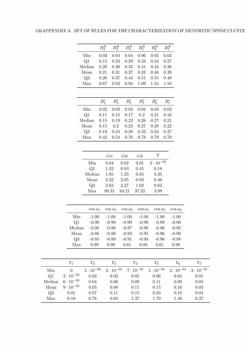
126APPENDIX A. SET OF RULES FOR THE CHARACTERIZATION OF DENDRITIC SPINE CLUSTERS
BR2 BR
3 BR4 BR
5 BR6 BR
7
Min 0.03 0.04 0.04 0.06 0.05 0.03Q1 0.15 0.23 0.29 0.33 0.34 0.27
Median 0.20 0.30 0.35 0.41 0.44 0.36Mean 0.21 0.31 0.37 0.42 0.46 0.39
Q3 0.26 0.37 0.44 0.51 0.55 0.48Max 0.67 0.82 0.94 1.09 1.24 1.16
Br2 Br
3 Br4 Br
5 Br6 Br
7
Min 0.02 0.03 0.03 0.04 0.03 0.03Q1 0.11 0.15 0.17 0.2 0.21 0.16
Median 0.15 0.19 0.22 0.26 0.27 0.21Mean 0.15 0.2 0.23 0.27 0.28 0.22
Q3 0.19 0.24 0.28 0.32 0.34 0.27Max 0.42 0.54 0.76 0.78 0.79 0.70
ϕ24 ϕ26 ϕ46 V
Min 0.04 0.02 0.01 2 · 10−03
Q1 1.32 0.83 0.45 0.18Median 1.85 1.25 0.65 0.35Mean 2.32 2.05 0.93 0.46
Q3 2.62 2.27 1.02 0.62Max 80.31 84.21 37.22 3.98
cosφ1 cosφ2 cosφ3 cosφ4 cosφ5 cosφ6
Min -1.00 -1.00 -1.00 -1.00 -1.00 -1.00Q1 -0.98 -0.99 -0.99 -0.99 -0.99 -0.98
Median -0.95 -0.96 -0.97 -0.98 -0.98 -0.95Mean -0.86 -0.90 -0.93 -0.95 -0.96 -0.90
Q3 -0.85 -0.89 -0.91 -0.94 -0.96 -0.88Max 0.99 0.99 0.61 0.88 0.61 0.98
V1 V2 V3 V4 V5 V6 V7
Min 0 5 · 10−06 3 · 10−04 7 · 10−04 5 · 10−04 2 · 10−04 3 · 10−05
Q1 2 · 10−03 0.02 0.03 0.05 0.06 0.04 0.01Median 6 · 10−03 0.04 0.06 0.09 0.11 0.09 0.02Mean 9 · 10−03 0.05 0.08 0.11 0.15 0.16 0.03
Q3 0.01 0.07 0.11 0.15 0.20 0.18 0.04Max 0.16 0.78 0.94 1.37 1.70 1.48 0.37

Appendix BProofs
B.1 Derivation of the Extended Mardia-Sutton distribution
To obtain a directional-linear distribution, Mardia and Sutton Mardia and Sutton [1978]
decomposed a trivariate normal distribution into a Gaussian distribution conditioned to
a bivariate Gaussian. Then, they transformed the bivariate Gaussian from Cartesian to
polar coordinates and restricted their parameters to construct the von Mises distribution
(see Equation (3.6)). We define the Extended Mardia-Sutton distribution following a similar
procedure.
First, we consider two disjoint sets of linear random variables Xa ∈ RL and Xb ∈ R2D,
where L is the number of linear variables and D is the number of directional variables. We
assume that Xa and Xb are distributed according to the following joint p.d.f.:
f
(Xa
Xb
)∼ N
[(Xa
Xb
);
(µa
µb
),
(Σaa Σab
Σba Σbb
)],
where µa ∈ RL and µb ∈ R2D are the means of Xa and Xb, respectively, Σaa is a matrix of
dimension L × L, Σab is a matrix of dimension L × 2D, Σba = ΣTab, and Σbb is a matrix of
dimension 2D × 2D.
Applying the chain rule of probability to the joint p.d.f. of the multivariate normal
distribution, the well-known expression for the conditional normal distribution is obtained
f
(Xa
Xb
)= f(Xb)f(Xa|Xb) = fN (Xb;µb,Σbb)fN (Xa;β0 + β>Xb,Q), (B.1)
where
β0 = µa −ΣabΣ−1bb µb,
β> = ΣabΣ−1bb ,
Q = Σaa −ΣabΣ−1bb Σba.
127
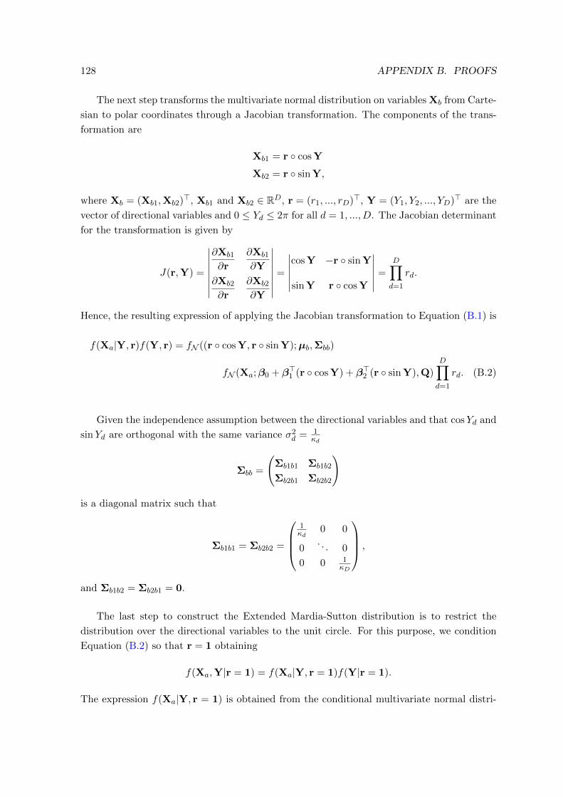
128 APPENDIX B. PROOFS
The next step transforms the multivariate normal distribution on variables Xb from Carte-
sian to polar coordinates through a Jacobian transformation. The components of the trans-
formation are
Xb1 = r ◦ cos Y
Xb2 = r ◦ sin Y,
where Xb = (Xb1,Xb2)>, Xb1 and Xb2 ∈ RD, r = (r1, ..., rD)>, Y = (Y1, Y2, ..., YD)> are the
vector of directional variables and 0 ≤ Yd ≤ 2π for all d = 1, ..., D. The Jacobian determinant
for the transformation is given by
J(r,Y) =
∣∣∣∣∣∣∣∣∂Xb1
∂r
∂Xb1
∂Y
∂Xb2
∂r
∂Xb2
∂Y
∣∣∣∣∣∣∣∣ =
∣∣∣∣∣∣cos Y −r ◦ sin Y
sin Y r ◦ cos Y
∣∣∣∣∣∣ =D∏d=1
rd.
Hence, the resulting expression of applying the Jacobian transformation to Equation (B.1) is
f(Xa|Y, r)f(Y, r) = fN ((r ◦ cos Y, r ◦ sin Y);µb,Σbb)
fN (Xa;β0 + β>1 (r ◦ cos Y) + β>2 (r ◦ sin Y),Q)
D∏d=1
rd. (B.2)
Given the independence assumption between the directional variables and that cosYd and
sinYd are orthogonal with the same variance σ2d = 1
κd
Σbb =
(Σb1b1 Σb1b2
Σb2b1 Σb2b2
)
is a diagonal matrix such that
Σb1b1 = Σb2b2 =
1κd
0 0
0. . . 0
0 0 1κD
,
and Σb1b2 = Σb2b1 = 0.
The last step to construct the Extended Mardia-Sutton distribution is to restrict the
distribution over the directional variables to the unit circle. For this purpose, we condition
Equation (B.2) so that r = 1 obtaining
f(Xa,Y|r = 1) = f(Xa|Y, r = 1)f(Y|r = 1).
The expression f(Xa|Y, r = 1) is obtained from the conditional multivariate normal distri-
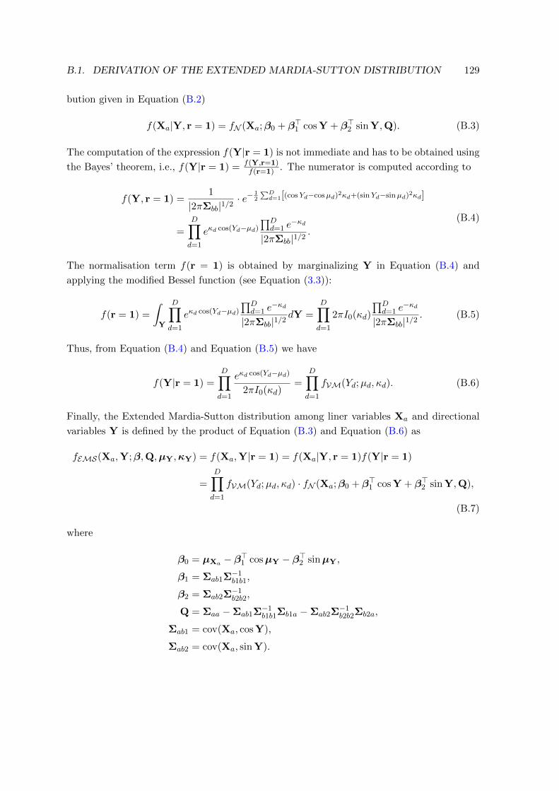
B.1. DERIVATION OF THE EXTENDED MARDIA-SUTTON DISTRIBUTION 129
bution given in Equation (B.2)
f(Xa|Y, r = 1) = fN (Xa;β0 + β>1 cos Y + β>2 sin Y,Q). (B.3)
The computation of the expression f(Y|r = 1) is not immediate and has to be obtained using
the Bayes’ theorem, i.e., f(Y|r = 1) = f(Y,r=1)f(r=1) . The numerator is computed according to
f(Y, r = 1) =1
|2πΣbb|1/2· e−
12
∑Dd=1[(cosYd−cosµd)2κd+(sinYd−sinµd)2κd]
=D∏d=1
eκd cos(Yd−µd)
∏Dd=1 e
−κd
|2πΣbb|1/2.
(B.4)
The normalisation term f(r = 1) is obtained by marginalizing Y in Equation (B.4) and
applying the modified Bessel function (see Equation (3.3)):
f(r = 1) =
∫Y
D∏d=1
eκd cos(Yd−µd)
∏Dd=1 e
−κd
|2πΣbb|1/2dY =
D∏d=1
2πI0(κd)
∏Dd=1 e
−κd
|2πΣbb|1/2. (B.5)
Thus, from Equation (B.4) and Equation (B.5) we have
f(Y|r = 1) =
D∏d=1
eκd cos(Yd−µd)
2πI0(κd)=
D∏d=1
fVM(Yd;µd, κd). (B.6)
Finally, the Extended Mardia-Sutton distribution among liner variables Xa and directional
variables Y is defined by the product of Equation (B.3) and Equation (B.6) as
fEMS(Xa,Y;β,Q,µY,κY) = f(Xa,Y|r = 1) = f(Xa|Y, r = 1)f(Y|r = 1)
=D∏d=1
fVM(Yd;µd, κd) · fN (Xa;β0 + β>1 cos Y + β>2 sin Y,Q),
(B.7)
where
β0 = µXa − β>1 cosµY − β>2 sinµY,
β1 = Σab1Σ−1b1b1,
β2 = Σab2Σ−1b2b2,
Q = Σaa −Σab1Σ−1b1b1Σb1a −Σab2Σ
−1b2b2Σb2a,
Σab1 = cov(Xa, cos Y),
Σab2 = cov(Xa, sin Y).
130 APPENDIX B. PROOFS
B.2 Bhattacharyya distance for the von Mises distribution
In this section we introduce the mathematical background needed to achieve a closed-form
equation for the Bhattacharyya distance between two univariate vM distributions. First,
the Bhattacharyya coefficient between two univariate vM distribution P (Yd) and Q(Yd) for
a directional random variable Yd is defined as
BC(P (Yd), Q(Yd)) =
∫ 2π
0
√P (Yd)Q(Yd)dYd. (B.8)
Then, Bhattacharyya distance is computed as
BD(P (Yd), Q(Yd)) = − lnBC(P (Yd), Q(Yd)).
Let define the following trigonometric identities that will be used during the derivation
of the Bhattacharyya distance
cos(x− y) = cos(x) cos(y) + sin(x) sin(y), (B.9)
and
a cos(x) + b cos(x) = R cos(x− α) (B.10)
where R =√a2 + b2 and tan(α) = b
a .
First of all we have to derive the Bhattacharyya coefficient (B.8) between two univariate
vM distributions as
BC(P (Yd), Q(Yd)) =
∫ 2π
0
√√√√eκPd cos(Yd−µPd )
2πI0(κPd )
eκQd cos(Yd−µQd )
2πI0(κQd )dYd
=1
2π√I0(κPd )I0(κQd )
∫ 2π
0eκPd2
cos(Yd−µPd )eκQd2
cos(Yd−µQd )dYd
where the means of both distributions are µPd and µQd and the concentration parameters are
κPd and κQd . To compute the integral part we apply the first trigonometric identity (B.9) and
rearrange the terms
1
2π√I0(κPd )I0(κQd )
∫ 2π
0eκPd2
(cos(Yd) cos(µPd )+sin(Yd) sin(µPd ))+κQd2
(cos(Yd) cos(µQd )+sin(Yd) sin(µQd ))
=1
2π√I0(κPd )I0(κQd )
∫ 2π
0ecos(Yd)(
κPd2
cos(µPd )+κQd2
cos(µQd ))+sin(Yd)(κPd2
sin(µPd )+κQd2
sin(µQd ))
B.3. KULLBACK-LEIBLER DIVERGENCE FOR THE VON MISES DISTRIBUTION131
Then, replacing according to
a =κPd2
cos(µPd ) +κQd2
cos(µQd )
b =κPd2
sin(µPd ) +κQd2
sin(µQd ),
we obtain1
2π√I0(κPd )I0(κQd )
∫ 2π
0ea cos(Yd)+b sin(Yd).
Applying the trigonometric identity (B.10) results:
1
2π√I0(κPd )I0(κQd )
∫ 2π
0eR cos(Yd−α)
where R =√a2 + b2 and tan(α) = b
a Finally, the closed-form expression for the Bhat-
tacharyya coefficient is obtained replacing the integral by the definition of modified Bessel
function (3.3) of first kind and order 0 so:
BC(P (Yd), Q(Yd)) =1
2π√I0(κPd )I0(κQd )
2πI0(R) =I0(R)√
I0(κPd )I0(κQd )(B.11)
The resulting expression for the Bhattacharyya distance is:
BD(P (Yd), Q(Yd)) = − lnBC(P (Yd), Q(Yd)) = − ln(I0(R)) +ln(I0(κPd )) + ln(I0(κPd ))
2(B.12)
B.3 Kullback-Leibler divergence for the von Mises distribu-
tion
The Kullback-Leibler divergence or relative entropy between two vM distributions P and Q
for a directional random variable Yd is defined as
DKL(P (Yd)||Q(Y )) = EP(
logP (Y )
Q(Y )
). (B.13)
To obtain a closed-form expression for the KL divergence between two univariate vM we start
by introducing the definitions of the modified Bessel function of the first kind and order n
for a directional variable Yd
In(κ) =1
2π
∫ 2π
0eκ cos(Yd) cos(nYd)dYd (B.14)
132 APPENDIX B. PROOFS
and the ratio between modified Bessel functions of order one and order zero
A(κ) =I1(κ)
I0(κ). (B.15)
Assume that we have two univariate von Mises distributions (Equation (3.2)) for the direc-
tional variable Yd, i.e.,
P (Yd) = fVM(Yd;µPd , κ
Pd ) and Q(Yd) = fVM(Yd;µ
Qd , κ
Qd ).
For the sake of simplicity, we rotate the directional variable Yd and the distributions P (Yd) and
Q(Yd) according to µPd . The directional variable after the rotation is defined as Y ∗d = Yd−µPd ,
and the rotated distributions p and q are defined as
p(Y ∗d ) = fVM(Y ∗d ;µpd, κpd) and q(Y ∗d ) = fVM(Y ∗d ;µqd, κ
qd),
where the means of both distributions are µpd = µPd − µPd = 0 and µqd = µQd − µPd and the
concentration parameters are obtained from κpd = κPd and κqd = κQd . Note that the rotation
does not change the concentration of the distributions. Then, the KL divergence between
univariate vM distributions is given by
DKL(p(Y ∗d )||q(Y ∗d )) =
∫ 2π
0p(Y ∗d ) log
p(Y ∗d )
q(Y ∗d )dY ∗d =
∫ 2π
0p(Y ∗d ) log
eκpd cos(Y ∗d )
I0(κpd)
I0(κqd)
eκqd cos(Y ∗d −µ
qd)dY ∗d .
Simplifying and applying the logarithm, we obtain∫ 2π
0p(Y ∗d )
[log I0(κqd)− log I0(κpd) + κpd cos(Y ∗d )− κqd cos(Y ∗d − µ
qd)]dY ∗d .
Thus, we have to compute four integrals. The first integral is:∫ 2π
0p(Y ∗d ) log I0(κqd)dY
∗d = log I0(κqd)
∫ 2π
0p(Y ∗d )dY ∗d = log I0(κqd),
as∫ 2π
0 p(Y ∗d )dY ∗d = 1. The second integral is obtained similarly:∫ 2π
0p(Y ∗d ) log I0(κpd)dY
∗d = log I0(κpd)
∫ 2π
0p(Y ∗d )dY ∗d = log I0(κpd).
To compute the third integral, we use Equations (3.3) and (B.15):∫ 2π
0p(Y ∗d )κp cos(Y ∗d )dY ∗d =
κp
2πI0(κpd)
∫ 2π
0eκ
pd cos(Y ∗d ) cos(Y ∗d )dY ∗d = κpdA(κpd).
B.4. KULLBACK-LEIBLER DIVERGENCE FOR THE EXTENDEDMARDIA-SUTTONDISTRIBUTION133
To compute the last integral, we again apply Equations (3.3) and (B.15):∫ 2π
0p(Y ∗d )κqd cos(Y ∗d − µ
qd)dY
∗d
=κqd
2πI0(κpd)
∫ 2π
0eκ
p cos(Y ∗d ) cos(Y ∗d − µq)dY ∗d
=κqd
2πI0(κpd)
∫ 2π
0eκ
p cos(Y ∗d )(cos(Y ∗d ) cos(µqd) + sin(Y ∗d ) sin(µqd))dY∗d
=κq
2πI0(κpd)
[cos(µqd)
∫ 2π
0eκ
pd cos(Y ∗d ) cos(Y ∗d )dY ∗d + sin(µqd)
∫ 2π
0eκ
pd cos(Y ∗d ) sin(Y ∗d )dY ∗d
]=
κqdI0(κpd)
cos(µqd)I1(κpd) = κqd cos(µqd)A(κpd).
Finally, joining the results of all the integrals, we obtain the closed-form
DKL(p(Y ∗d )||q(Y ∗d )) = log I0(κqd)− log I0(κpd) +A(κpd)(κpd − κ
qd cos(µqd)
). (B.16)
B.4 Kullback-Leibler divergence for the Extended Mardia-
Sutton distribution
The Kullback-Leibler divergence or relative entropy between two Extended Mardia-Sutton
distributions P and Q is defined as
DKL(P (X,Y)||Q(X,Y)) = EP(
logP (X,Y)
Q(X,Y)
), (B.17)
which can be factorised according to Equation (B.7) as
DKL(P (X,Y)||Q(X,Y)) =
D∑d=1
DKL(P (Yd)||Q(Yd)) +DKL(P (X|PaGX)||Q(X|PaGX)). (B.18)
Hence, the KL divergence decomposes as a sum of independent KL divergences between
univariate von Mises distributions B.3 and the KL divergence of the linear variables condi-
tioned to the directional variables. In the next subsections, we derive the two types of KL
terms.
B.4.1 Conditional Kullback-Leibler divergence of the Extended Mardia-
Sutton distribution
The KL divergence of the linear variables conditioned to the directional variables between
the Extended Mardia-Sutton distributions P and Q is defined as
DKL(P (X|PaGX)||Q(X|PaGX)) =
∫Y
D∏d=1
P (Yd)DKL(P (X|Y)||Q(X|Y))dY. (B.19)

134 APPENDIX B. PROOFS
Given that the linear variables are distributed according to a multivariate normal distribu-
tion (see Equation (B.7)), the multivariate normal KL divergence can be computed according
to the well-known equation
DKL(P (X|Y)||Q(X|Y)) =1
2
[Tr(Σ−1,QΣP ) + (µQ − µP )>Σ−1,Q(µQ − µP )− L+ ln
|ΣQ||ΣP |
],
(B.20)
where L is the number of linear variables.
There are four additive terms. The first, the third and the fourth terms are constant with
respect to Y, so
∫Y
D∏d=1
fVM(Yd;µPd , κ
Pd )·1
2
[Tr(Σ−1,QΣP )− L+ ln
|ΣQ||ΣP |
]dY =
1
2
[Tr(Σ−1,QΣP )− L+ ln
|ΣQ||ΣP |
]
Let us define µR = µQ − µP as
µR = (βQ0 − βP0 ) + (βQ1 − βP1 )> cos Y + (βQ2 − βP2 )> sin Y = βR0 + βR1>
cos Y + βR2>
sin Y.
The second term in the multivariate normal KL divergence (see Equation (B.20)) is a quadratic
form that can be written as∫Y
D∏d=1
fVM(Yd;µPd , κ
Pd )
(L∑
i,j=1
Σ−1,Qij µRi µ
Rj
)dY =
∫Y
D∏d=1
fVM(Yd;µPd , κ
Pd )
(L∑
i,j=1
Σ−1,Qij (βR0i + βR1i
>cos Y + βR2i
>sin Y)(β0j + βR1j
>cos Y + βR2j
>sin Y)
)dY.
where Σ−1,Qij is the element at the i-th row and j-th column in Σ−1,Q and µRi and µRj are the
i-th and j-th components of vector µR. Then, we compute the integrals over each additive
term, applying Equation (3.3) and some well-known trigonometric identities to yield
∫Y
D∏d=1
fVM(Yd;µPd , κ
Pd )
L∑i,j=1
Σ−1,Qij βR0iβ
R0j
dY =
L∑i,j=1
Σ−1,Qij βR0iβ
R0j ,
∫Y
D∏d=1
fVM(Yd;µPd , κ
Pd ) ·
L∑i,j=1
Σ−1,Qij βR0i(β
R1j>
cos Y)
dY =L∑
i,j=1
Σ−1,Qij βR0i
D∑d=1
βR1jdA(κPd ),
∫Y
D∏d=1
fVM(Yd;µPd , κ
Pd ) ·
L∑i,j=1
Σ−1,Qij βR0j(β
R1i>
cos Y)
dY =
L∑i,j=1
Σ−1,Qij βR0j
D∑d=1
βR1idA(κPd ),

B.4. KULLBACK-LEIBLER DIVERGENCE FOR THE EXTENDEDMARDIA-SUTTONDISTRIBUTION135
∫Y
D∏d=1
fVM(Yd;µPd , κ
Pd ) ·
L∑i,j=1
Σ−1,Qij (βR1i
>cos Y)(βR1j
>cos Y)
dY
=
L∑i,j=1
Σ−1,Qij
(D∑d=1
βR1idβR1jd
2·(
1 +I2(κPd )
I0(κPd )
)+
D∑d=1
D∑m6=d
βR1idβR1jmA(κPd )A(κPm)
),
and
∫Y
D∏d=1
fVM(Yd;µPd , κ
Pd ) ·
L∑i,j=1
Σ−1,Qij (βR2i
>sin Y)(βR2j
>sin Y)
dY
=L∑
i,j=1
Σ−1,Qij
D∑d=1
βR2idβR2jd
2
(1−
I2(κPd )
I0(κPd )
).
We omit those terms whose result of solving the integral was always zero. Finally, grouping
all of the terms in one equation, we obtain the expression for the conditional KL divergence
DKL(P (X|PaGX)||Q(X|PaGX)) =1
2
L∑i,j=1
Σ−1,Qij
[βR0iβ
R0j + 2βR0i
D∑d=1
βR1jdA(κPd )
+D∑d=1
βR1idβR1jd
2
(1 +
I2(κPd )
I0(κPd )
)+
D∑d=1
D∑m6=d
βR1idβR1jmA(κPd )A(κPm) +
D∑d=1
βR2idβR2jd
2
(1−
I2(κPd )
I0(κPd )
)]+
1
2
[Tr(Σ−1,QΣP )− L+ ln
|ΣQ||ΣP |
].

136 APPENDIX B. PROOFS
Bibliography
L. Abbott. Firing-rate models for neural populations. In Neural Networks: From Biology to
High Energy Physics: Proceedings of the Second Workshop, pages 179–196. World Scientific,
1991.
T. Abe and C. Ley. A tractable, parsimonious and flexible model for cylindrical data, with
applications. Econometrics and Statistics, 4:91–104, 2017.
Abou-Moustafa and F. P. Ferrie. A note on metric properties of some divergence measures:
The Gaussian case. In Proceedings of Machine Learning Research, volume 25, pages 1–12,
1995.
M. Abramowitz and I. A. Stegun. Handbook of Mathematical Functions. Dover, 1970.
H. Akaike. A new look at the statistical model identification. IEEE Transactions on Auto-
matic Control, 19(6):716–723, 1974.
A. Alavi, B. Cavanagh, G. Tuxworth, A. Meedeniya, A. Mackay-Sim, and M. Blumenstein.
Automated classification of dopaminergic neurons in the rodent brain. In Proceedings of
the 2009 International Joint Conference on Neural Networks, pages 81–88. IEEE Press,
2009.
J. I. Alonso-Barba, L. delaOssa, and J. M. Puerta. Structural learning of Bayesian networks
using local algorithms based on the space of orderings. Soft Computing, 15(10):1881–1895,
2011.
H. Anwar, I. Riachi, S. Hill, F. Schurmann, and H. Markram. An approach to capturing
neuron morphological diversity. In Computational Modeling Methods for Neuroscientists,
pages 211–231. The MIT Press, 2009.
R. Araya. Input transformation by dendritic spines of pyramidal neurons. Frontiers in
Neuroanatomy, 8, 2014. doi: 10.3389/fnana.2014.00141.
R. Araya. Dendritic morphology and function. In Neuroscience in the 21st Century: From
Basic to Clinical, pages 297–331. Springer, 2016.
R. Araya, T. P. Vogels, and R. Yuste. Activity-dependent dendritic spine neck changes are
correlated with synaptic strength. Proceedings of the National Academy of Sciences, 111
(28):2895–2094, 2014.
137

138 BIBLIOGRAPHY
J. I. Arellano, R. Benavides-Piccione, J. DeFelipe, and R. Yuste. Ultrastructure of dendritic
spines: Correlation between synaptic and spine morphologies. Frontiers in Neuroscience,
1, 2007. doi: 10.3389/neuro.01.1.1.010.2007.
G. A. Ascoli. Progress and perspectives in computational neuroanatomy. The Anatomical
Record, 257(6):195–207, 1999.
G. A. Ascoli. Computational Neuroanatomy: Principles and Methods. Springer Science &
Business Media, 2002.
G. A. Ascoli. Mobilizing the base of neuroscience data: The case of neuronal morphologies.
Nature Reviews Neuroscience, 7:318–324, 2006.
G. A. Ascoli and J. L. Krichmar. L-Neuron: A modeling tool for the efficient generation and
parsimonious description of dendritic morphology. Neurocomputing, 32:1003–1011, 2000.
G. A. Ascoli, J. L. Krichmar, R. Scorcioni, S. J. Nasuto, S. L. Senft, and G. Krichmar.
Computer generation and quantitative morphometric analysis of virtual neurons. Anatomy
and Embryology, 204(4):283–301, 2001.
Y. Baba. Statistics of angular data: Wrapped normal distribution model. Proceedings of the
Institute of Statistical Mathematics, 28(1):41–54, 1981.
A. Banerjee, I. Dhillon, J. Ghosh, and S. Sra. Clustering on the unit hypersphere using von
Mises-Fisher distributions. Journal of Machine Learning Research, 6:1345–1382, 2005.
S. Basu, P. K. Saha, M. Roszkowska, M. Magnowska, E. Baczynska, N. Das, D. Plewczynski,
and J. Wlodarczyk. Quantitative 3-D morphometric analysis of individual dendritic spines.
Scientific Reports, 8(1):3545, 2018.
E. Batschelet. Circular Statistics in Biology. Academic Press, 1981.
E. Batschelet, D. Hillman, M. Smolensky, and F. Halberg. Angular-linear correlation coeffi-
cient for rhythmometry and circannually changing human birth rates at different geographic
latitudes. International Journal of Chronobiology, 1(55):183–202, 1973.
R. Benavides-Piccione, I. Ballesteros-Yanez, J. DeFelipe, and R. Yuste. Cortical area and
species differences in dendritic spine morphology. Journal of Neurocytology, 31(3-5):337–
346, 2002.
R. Benavides-Piccione, I. Fernaud-Espinosa, V. Robles, R. Yuste, and J. DeFelipe. Age-
based comparison of human dendritic spine structure using complete three-dimensional
reconstructions. Cerebral Cortex, 23(8):1798–1810, 2012.
R. Benavides-Piccione, I. Fernaud-Espinosa, V. Robles, R. Yuste, and J. DeFelipe. Age-
based comparison of human dendritic spine structure using complete three-dimensional
reconstructions. Cerebral Cortex, 23:1798–1810, 2013.
BIBLIOGRAPHY 139
M. Benjumeda, S. Luengo-Sanchez, P. Larranaga, and C. Bielza. Tractable learning of
Bayesian networks from partially observed data. Pattern Recognition, 91:190–199, 2019.
J. Bentley. Modelling Circular Data Using a Mixture of von Mises and Uniform Distributions.
PhD thesis, Department of Statistics and Actuarial Science-Simon Fraser University, 2006.
K. P. Berry and E. Nedivi. Spine dynamics: Are they all the same? Neuron, 96(1):43–55,
2017.
D. Best and N. Fisher. The BIAS of the maximum likelihood estimators of the von Mises-
Fisher concentration parameters. Communications in Statistics-Simulation and Computa-
tion, 10(5):493–502, 1981.
T. Beuzen, L. Marshall, and K. D. Splinter. A comparison of methods for discretizing con-
tinuous variables in Bayesian networks. Environmental Modelling & Software, 108:61–66,
2018.
A. Bhattacharyya. On a measure of divergence between two multinomial populations.
Sankhya: The Indian Journal of Statistics, 7(4):401–406, 1946.
B. Bidyuk and R. Dechter. Cutset sampling for Bayesian networks. Journal of Artificial
Intelligence Research, 28:1–48, 2007.
C. Bielza and P. Larranaga. Bayesian networks in neuroscience: A survey. Frontiers in
Computational Neuroscience, 8:131, 2014. doi: 10.3389/fncom.2014.00131.
C. M. Bishop. Pattern Recognition and Machine Learning. Springer, 2006.
R. Blanco, I. Inza, and P. Larranaga. Learning Bayesian networks in the space of structures
by estimation of distribution algorithms. International Journal of Intelligent Systems, 18
(2):205–220, 2003.
G. Bokota, M. Magnowska, T. Kusmierczyk, M. Lukasik, M. Roszkowska, and P. Dariusz.
Computational approach to dendritic spine taxonomy and shape transition analysis. Fron-
tiers in Computational Neuroscience, 10:140, 2016. doi: 10.3389/fncom.2016.00140.
T. Bonhoeffer and R. Yuste. Spine motility: Phenomenology, mechanisms, and function.
Neuron, 35(6):1019–1027, 2002.
W. Boomsma, J. T. Kent, K. V. Mardia, C. C. Taylor, and T. Hamelryck. Graphical models
and directional statistics capture protein structure. Interdisciplinary Statistics and Bioin-
formatics, 25:91–94, 2006.
W. Boomsma, K. V. Mardia, C. C. Taylor, J. Ferkinghoff-Borg, A. Krogh, and T. Hamelryck.
A generative, probabilistic model of local protein structure. Proceedings of the National
Academy of Sciences, 105(26):8932–8937, 2008.
140 BIBLIOGRAPHY
R. R. Bouckaert. Bayesian Belief Networks: From Construction to Inference. PhD thesis,
Faculteit Wiskunde en Informatica, Universiteit Utrecht, 1995.
J. Brito, S. Mata, S. Bayona, L. Pastor, J. DeFelipe, and R. Benavides Piccione. Neuronize:
A tool for building realistic neuronal cell morphologies. Frontiers in Neuroanatomy, 7:15,
2013. doi: 10.3389/fnana.2013.00015.
F. Bromberg, D. Margaritis, and V. Honavar. Efficient Markov network structure discovery
using independence tests. Journal of Artificial Intelligence Research, 35:449–484, 2009.
S. A. Buffington, J. M. Sobotzik, C. Schultz, and M. N. Rasband. Iκbα is not required for
axon initial segment assembly. Molecular and Cellular Neuroscience, 50(1):1–9, 2012.
P. Buhlmann, M. Kalisch, and M. H. Maathuis. Variable selection in high-dimensional linear
models: Partially faithful distributions and the PC-simple algorithm. Biometrika, 97(2):
261–278, 2010.
J. Bulla, F. Lagona, A. Maruotti, and M. Picone. A multivariate hidden Markov model for
the identification of sea regimes from incomplete skewed and circular time series. Journal
of Agricultural, Biological, and Environmental Statistics, 17(4):544–567, 2012.
S. Calderara, R. Cucchiara, and A. Prati. Detection of abnormal behaviors using a mixture
of von Mises distributions. In IEEE Conference on Advanced Video and Signal Based
Surveillance, 2007, pages 141–146. IEEE Press, 2007.
S. Calderara, A. Prati, and R. Cucchiara. Mixtures of von Mises distributions for people tra-
jectory shape analysis. IEEE Transactions on Circuits and Systems for Video Technology,
21(4):457–471, 2011.
J. A. Carta, P. Ramırez, and C. Bueno. A joint probability density function of wind speed and
direction for wind energy analysis. Energy Conversion and Management, 49(6):1309–1320,
2008.
E. Castillo, J. M. Gutierrez, and A. S. Hadi. Expert Systems and Probabilistic Network
Models. Springer Science & Business Media, 1996.
N. V. Chawla, K. W. Bowyer, L. O. Hall, and W. P. Kegelmeyer. Smote: Synthetic minority
over-sampling technique. Journal of Artificial Intelligence Research, 16(1):321–357, 2002.
S. H. Chen and C. A. Pollino. Good practice in Bayesian network modelling. Environmental
Modelling & Software, 37:134–145, 2012.
D. Chickering, D. Geiger, and D. Heckerman. Learning Bayesian networks: Search methods
and experimental results. In Proceedings of 5th Conference on Artificial Intelligence and
Statistics, pages 112–128, 1996.

BIBLIOGRAPHY 141
A. Choi and A. Darwiche. On the relative expressiveness of Bayesian and neural networks.
In Proceedings of the 9th International Conference on Probabilistic Graphical Models, vol-
ume 72, pages 157–168. Proceedings of Machine Learning Research, 2018.
P. S. Churchland and T. J. Sejnowski. The Computational Brain. The MIT Press, 1992.
P. Cignoni, C. Rocchini, and R. Scopigno. Metro: Measuring error on simplified surfaces.
Computer Graphics Forum, 17(2):167–174, 1998.
P. Cignoni, M. Callieri, M. Corsini, M. Dellepiane, F. Ganovelli, and G. Ranzuglia. MeshLab:
An open-source mesh processing tool. In Eurographics Italian Chapter Conference, pages
129–136. The Eurographics Association, 2008.
D. L. Clark, N. N. Boutros, and M. F. Mendez. The Brain and Behavior: An Introduction
to Behavioral Neuroanatomy. Cambridge University Press, 2005.
B. R. Cobb and P. P. Shenoy. Inference in hybrid Bayesian networks with mixtures of
truncated exponentials. International Journal of Approximate Reasoning, 41(3):257–286,
2006.
W. Cohen. Fast effective rule induction. In Proceedings of the 20th International Conference
on Machine Learning, pages 115–123. Morgan Kaufmann, 1995.
D. Collett and T. Lewis. Discriminating between the von Mises and wrapped normal distri-
butions. Australian Journal of Statistics, 23(1):73–79, 1981.
G. F. Cooper. The computational complexity of probabilistic inference using Bayesian belief
networks. Artificial Intelligence, 42(2):393–405, 1990.
G. F. Cooper and E. Herskovits. A Bayesian method for the induction of probabilistic
networks from data. Machine Learning, 9(4):309–347, 1992.
L. d. F. Costa, E. T. M. Manoel, F. Faucereau, J. Chelly, J. van Pelt, and G. Ramakers.
A shape analysis framework for neuromorphometry. Network: Computation in Neural
Systems, 13(3):283–310, 2002.
T. M. Cover and J. A. Thomas. Elements of Information Theory. John Wiley & Sons, 1991.
N. Cressie and C. K. Wikle. Statistics for Spatio-Temporal Data. John Wiley & Sons, 2015.
H. Cuntz, M. W. Remme, and B. Torben-Nielsen. The Computing Dendrite: From Structure
to Function. Springer Science & Business Media, 2014.
R. Daly, Q. Shen, and S. Aitken. Learning Bayesian networks: Approaches and issues. The
Knowledge Engineering Review, 26(2):99–157, 2011.
A. Darwiche. Recursive conditioning. Artificial Intelligence, 126(1):5–41, 2001.
142 BIBLIOGRAPHY
A. Darwiche. Modeling and Reasoning with Bayesian Networks. Cambridge University Press,
2009.
P. Dayan and L. F. Abbott. Theoretical Neuroscience: Computational and Mathematical
Modeling of Neural Systems. The MIT Press, 2001.
R. Dechter. Reasoning with Probabilistic and Deterministic Graphical Models: Exact Algo-
rithms. Morgan & Claypool Publishers, 2013.
J. DeFelipe and I. Farinas. The pyramidal neuron of the cerebral cortex: Morphological and
chemical characteristics of the synaptic inputs. Progress in Neurobiology, 39(6):563–607,
1992.
J. DeFelipe, P. L. Lopez-Cruz, R. Benavides-Piccione, C. Bielza, P. Larranaga, S. Anderson,
A. Burkhalter, B. Cauli, A. Fairen, D. Feldmeyer, G. Fishell, D. Fitzpatrick, T. F. Freund,
G. Gonzalez-Burgos, S. Hestrin, S. Hill, P. R. Hof, J. Huang, E. G. Jones, Y. Kawaguchi,
Z. Kisvarday, Y. Kubota, D. A. Lewis, O. Marın, H. Markram, C. J. McBain, H. S.
Meyer, H. Monyer, S. B. Nelson, K. Rockland, J. Rossier, J. L. R. Rubenstein, B. Rudy,
M. Scanziani, G. M. Shepherd, C. C. Sherwood, J. F. Staiger, G. Tamas, A. Thomson,
Y. Wang, R. Yuste, and G. A. Ascoli. New insights into the classification and nomenclature
of cortical GABAergic interneurons. Nature Reviews Neuroscience, 14(3):202–216, 2013.
A. Dempster, N. Laird, and D. Rubin. Maximum likelihood from incomplete data via the
EM algorithm. Journal of the Royal Statistical Society. Series B, 1:1–38, 1977.
M. Desbrun, M. Meyer, P. Schroder, and A. H. Barr. Implicit fairing of irregular meshes
using diffusion and curvature flow. In Proceedings of the 26th Annual Conference on Com-
puter Graphics and Interactive Techniques, pages 317–324. ACM Press/Addison-Wesley
Publishing Co., 1999.
M. Di Marzio, A. Panzera, and C. C. Taylor. Non-parametric regression for circular responses.
Scandinavian Journal of Statistics, 40(2):238–255, 2013.
B. Dickerson and A. Atri. Dementia: Comprehensive Principles and Practices. Oxford
University Press, 2014.
D. Dimitriu, J. Hao, Y. Hara, J. Kaufmann, W. G. M. Janssen, W. Lou, P. R. Rapp, and
M. J. H. Selective changes in thin spine density and morphology in monkey prefrontal
cortex correlate with aging-related cognitive impairment. Journal of Neuroscience, 30(20):
7507–7515, 2010.
D. E. Donohue and G. A. Ascoli. A comparative computer simulation of dendritic morphology.
PLOS Computational Biology, 4(6):e1000089, 2008.
D. E. Donohue, R. Scorcioni, and G. A. Ascoli. Generation and description of neuronal
morphology using L-neuron. In Computational Neuroanatomy: Principles and Methods,
pages 49–69. Humana Press, 2002.

BIBLIOGRAPHY 143
A. Doucet, N. d. Freitas, K. P. Murphy, and S. J. Russell. Rao-Blackwellised particle filtering
for dynamic Bayesian networks. In Proceedings of the 16th Conference on Uncertainty in
Artificial Intelligence, pages 176–183. Morgan Kaufmann Publishers Inc., 2000.
J. Dougherty, R. Kohavi, and M. Sahami. Supervised and unsupervised discretization of con-
tinuous features. In Proceedings of the 12th International Conference on Machine Learning,
pages 194–202. Elsevier, 1995.
R. Duda, P. Hart, and D. Stork. Pattern Classification. Wiley Interscience, 2001.
A. Dunaevsky, A. Tashiro, A. Majewska, C. Mason, and R. Yuste. Developmental regulation
of spine motility in the mammalian central nervous system. Proceedings of the National
Academy of Sciences, 96(23):13438–13443, 1999.
G. Elidan, N. Lotner, N. Friedman, and D. Koller. Discovering hidden variables: A structure-
based approach. In Advances in Neural Information Processing Systems, pages 479–485,
2001.
B. Eltzner, S. Huckemann, and K. V. Mardia. Torus principal component analysis with
applications to RNA structure. The Annals of Applied Statistics, 12(2):1332–1359, 2018.
R. Etxeberria, P. Larranaga, and J. M. Picaza. Analysis of the behaviour of genetic algorithms
when learning Bayesian network structure from data. Pattern Recognition Letters, 18(11-
13):1269–1273, 1997.
G. Eyal, M. B. Verhoog, G. Testa-Silva, Y. Deitcher, J. C. Lodder, R. Benavides-Piccione,
J. Morales, J. DeFelipe, C. P. de Kock, H. D. Mansvelder, and I. Segev. Unique membrane
properties and enhanced signal processing in human neocortical neurons. eLife, 5(e16553),
2016.
G. Eyal, M. B. Verhoog, G. Testa-Silva, Y. Deitcher, R. Benavides-Piccione, J. DeFelipe,
C. P. J. de Kock, H. D. Mansvelder, and I. Segev. Human cortical pyramidal neurons:
From spines to spikes via models. Frontiers in Cellular Neuroscience, 12:181, 2018. doi:
10.3389/fncel.2018.00181.
E. Faulkner. K2GA: Heuristically guided evolution of Bayesian network structures from data.
In 2007 IEEE Symposium on Computational Intelligence and Data Mining, pages 18–25.
IEEE Press, 2007.
U. Fayyad and K. Irani. Multi-interval discretization of continuous valued attributes for clas-
sification learning. In Proceedings of the 13th International Joint Conference on Artificial
Intelligence, pages 1022–1027. Morgan Kaufmann Publishers Inc., 1993.
N. Fisher and A. Lee. Time series analysis of circular data. Journal of the Royal Statistical
Society: Series B (Methodological), 56(2):327–339, 1994.
144 BIBLIOGRAPHY
N. I. Fisher and A. J. Lee. Regression models for an angular response. Biometrics, 48(3):
665–677, 1992.
R. Fisher. Dispersion on a sphere. Proceedings of the Royal Society of London. Series A,
Mathematical and Physical Sciences, 217(110):295–305, 1953.
C. Fraley and A. Raftery. Model-based clustering, discriminant analysis, and density estima-
tion. Journal of the American Statistical Association, 97(458):611–631, 2002.
N. Friedman. Learning belief networks in the presence of missing values and hidden variables.
In Proceedings of the 14th International Conference on Machine Learning, volume 97, pages
125–133. Elsevier, 1997.
N. Friedman and M. Goldszmidt. Discretizing continuous attributes while learning Bayesian
networks. In Proceedings of the 13th International Conference on International Conference
on Machine Learning, pages 157–165. Morgan Kaufmann Publishers Inc., 1996.
N. Friedman and I. Nachman. Gaussian process networks. In Proceedings of the 16th Confer-
ence on Uncertainty in Artificial Intelligence, pages 211–219. Morgan Kaufmann Publishers
Inc., 2000.
N. Friedman, I. Nachman, and D. Peer. Learning Bayesian network structure from massive
datasets: The “sparse candidate” algorithm. In Proceedings of the 15th conference on
Uncertainty in Artificial Intelligence, pages 206–215. Morgan Kaufmann Publishers Inc.,
1999.
K. Fukunaga. Introduction to Statistical Pattern Recognition. Elsevier, 1972.
J. A. Gamez, J. L. Mateo, and J. M. Puerta. Learning Bayesian networks by hill climbing:
Efficient methods based on progressive restriction of the neighborhood. Data Mining and
Knowledge Discovery, 22(1-2):106–148, 2011.
R. Gatto. Some computational aspects of the generalized von Mises distribution. Statistics
and Computing, 18(3):321–331, 2008.
R. Gatto and S. R. Jammalamadaka. The generalized von Mises distribution. Statistical
Methodology, 4(3):341–353, 2007.
D. Geiger and D. Heckerman. Learning Gaussian networks. In Proceedings of the 10th
International Conference on Uncertainty in Artificial Intelligence, pages 235–243. Morgan
Kaufmann Publishers Inc., 1994.
F. Gelfo, P. De Bartolo, A. Giovine, L. Petrosini, and M. G. Leggio. Layer and regional effects
of environmental enrichment on the pyramidal neuron morphology of the rat. Neurobiology
of Learning and Memory, 91(4):353–365, 2009.
C. R. Gerfen, M. N. Economo, and J. Chandrashekar. Long distance projections of cortical
pyramidal neurons. Journal of Neuroscience Research, 96(9):1467–1475, 2018.

BIBLIOGRAPHY 145
M. U. Ghani, E. Erdil, S. D. Kanik, A. O. Argunsah, A. F. Hobbiss, I. Israely, D. Unay,
T. Tasdizen, and M. Cetin. Dendritic spine shape analysis: A clustering perspective.
In Proceedings of Computer Vision – ECCV 2016 Workshops, pages 256–273. Springer
International Publishing, 2016.
W. R. Gilks, S. Richardson, and D. Spiegelhalter. Markov Chain Monte Carlo in Practice.
Chapman and Hall/CRC, 1996.
J. R. Glaser and E. M. Glaser. Neuron imaging with Neurolucida - A PC-based system for
image combining microscopy. Computerized Medical Imaging and Graphics, 14(5):307–317,
1990.
F. Glover, M. Laguna, E. Taillard, and D. de Werra. Tabu Search. Springer, 1993.
U. Gordon, A. Polsky, and J. Schiller. Plasticity compartments in basal dendrites of neocor-
tical pyramidal neurons. Journal of Neuroscience, 26(49):12717–12726, 2006.
N. A. Goriounova, D. B. Heyer, R. Wilbers, M. B. Verhoog, M. Giugliano, C. Verbist, J. Ober-
mayer, A. Kerkhofs, H. Smeding, M. Verberne, S. Idema, J. C. Baayen, A. W. Pieneman,
C. P. de Kock, M. Klein, and H. D. Mansvelder. Large and fast human pyramidal neurons
associate with intelligence. eLife, 7, 2018. doi: 10.7554/eLife.41714.
A. L. Gould. A regression technique for angular variates. Biometrics, 25(4):683–700, 1969.
L. Guerra, L. M. McGarry, V. Robles, C. Bielza, P. Larranaga, and R. Yuste. Comparison
between supervised and unsupervised classifications of neuronal cell types: A case study.
Developmental Neurobiology, 71(1):71–82, 2011.
S. Guiasu and A. Shenitzer. The principle of maximum entropy. The Mathematical Intelli-
gencer, 7(1):42–48, 1985.
E. J. Gumbel, J. A. Greenwood, and D. Durand. The circular normal distribution: Theory
and tables. Journal of the American Statistical Association, 48(261):131–152, 1953.
M. Hall, E. Frank, G. Holmes, B. Pfahringer, P. Reutemann, and I. H. Witten. The WEKA
data mining software: An update. SIGKDD Explorations, 11(1):10–18, 2009.
T. Hamelryck, K. Mardia, and J. Ferkinghoff-Borg. Bayesian Methods in Structural Bioin-
formatics. Springer, 2012.
T. Harder, W. Boomsma, M. Paluszewski, J. Frellsen, K. E. Johansson, and T. Hamelryck.
Beyond rotamers: A generative, probabilistic model of side chains in proteins. BMC
Bioinformatics, 11(1):306, 2010. doi: 10.1186/1471-2105-11-306.
K. D. Harris and G. M. Shepherd. The neocortical circuit: Themes and variations. Nature
Neuroscience, 18(2):170–181, 2015.
146 BIBLIOGRAPHY
K. M. Harris and J. K. Stevens. Dendritic spines of rat cerebellar Purkinje cells: Serial electron
microscopy with reference to their biophysical characteristics. Journal of Neuroscience, 8
(12):4455–4469, 1988.
K. M. Harris and J. K. Stevens. Dendritic spines of CA1 pyramidal cells in the rat hippocam-
pus: Serial electron microscopy with reference to their biophysical characteristics. Journal
of Neuroscience, 9(8):2982–2997, 1989.
M. Hausser and B. Mel. Dendrites: Bug or feature? Current Opinion in Neurobiology, 13
(3):372–383, 2003.
D. Heckerman, D. Geiger, and D. Chickering. Learning Bayesian networks: The combination
of knowledge and statistical data. Machine Learning, 20:197–243, 1995.
T. Heiberg, B. Kriener, T. Tetzlaff, G. T. Einevoll, and H. E. Plesser. Firing-rate mod-
els for neurons with a broad repertoire of spiking behaviors. Journal of Computational
Neuroscience, 45(2):103–132, 2018.
S. H. C. Hendry and E. G. Jones. The organization of pyramidal and non-pyramidal cell den-
drites in relation to thalamic afferent terminations in the monkey somatic sensory cortex.
Journal of Neurocytology, 13(1):277–298, 1983.
J. Hernandez-Gonzalez, I. Inza, and J. A. Lozano. Learning Bayesian network classifiers from
label proportions. Pattern Recognition, 46(12):3425–3440, 2013.
D. Hernandez-Stumpfhauser, F. J. Breidt, and M. J. van der Woerd. The general projected
normal distribution of arbitrary dimension: Modeling and Bayesian inference. Bayesian
Analysis, 12(1):113–133, 2017.
M. Hilaga, Y. Shinagawa, T. Kohmura, and T. Kunii. Topology matching for fully automatic
similarity estimation of 3D shapes. In Proceedings of the 28th Annual Conference on
Computer Graphics and Interactive Techniques, pages 203–212. ACM, 2001.
P. R. Hof and J. H. Morrison. The aging brain: Morphomolecular senescence of cortical
circuits. Trends in Neurosciences, 27(10):607–613, 2004.
R. Hofmann and V. Tresp. Discovering structure in continuous variables using Bayesian
networks. In Proceedings of the 9th Conference on Neural Information Processing Systems,
pages 500–506, 1996.
J. H. Holland. Adaptation in Natural and Artificial Systems: An Introductory Analysis with
Applications to Biology, Control, and Artificial Intelligence. The MIT Press, 1992.
A. Holtmaat and K. Svoboda. Experience-dependent structural synaptic plasticity in the
mammalian brain. Nature Reviews Neuroscience, 10(9):647–658, 2009.
BIBLIOGRAPHY 147
W. H. Hsu, H. Guo, B. B. Perry, and J. A. Stilson. A permutation genetic algorithm for
variable ordering in learning Bayesian networks from data. In Proceedings of the 4th Annual
Conference on Genetic and Evolutionary Computation, pages 383–390. Morgan Kaufmann
Publishers Inc., 2002.
T. S. Jaakkola and Y. Qi. Parameter expanded variational Bayesian methods. In Advances
in Neural Information Processing Systems, pages 1097–1104, 2007.
B. Jacobs, L. Driscoll, and M. Schall. Life-span dendritic and spine changes in areas 10 and
18 of human cortex: A quantitative Golgi study. Journal of Comparative Neurology, 386
(4):661–680, 1997.
S. R. Jammalamadaka and A. Sengupta. Topics in Circular Statistics. World Scientific, 2001.
E. Jaynes. Information theory and statistical mechanics. Physical Review, 106:620–630, 1957.
F. Jensen, S. Lauritzen, and K. Olsen. Bayesian updating in recursive graphical models by
local computation. Computational Statistics Quarterly, 4:269–282, 1990.
R. A. Johnson and T. E. Wehrly. Some angular-linear distributions and related regression
models. Journal of the American Statistical Association, 73(363):602–606, 1978.
M. I. Jordan, Z. Ghahramani, T. S. Jaakkola, and L. K. Saul. An introduction to variational
methods for graphical models. Machine Learning, 37(2):183–233, 1999.
M. Kalisch and P. Buhlmann. Estimating high-dimensional directed acyclic graphs with the
PC-algorithm. Journal of Machine Learning Research, 8:613–636, 2007.
M. Kalisch and P. Buhlmann. Robustification of the PC-algorithm for directed acyclic graphs.
Journal of Computational and Graphical Statistics, 17(4):773–789, 2008.
H. Kasai, M. Fukuda, S. Watanabe, A. Hayashi-Takagi, and J. Noguchi. Structural dynamics
of dendritic spines in memory and cognition. Trends in Neurosciences, 33(3):121–129, 2010.
P. Kasarapu. Modelling of directional data using Kent distributions. CoRR, abs/1506.08105.
S. Kato and M. Jones. A family of distributions on the circle with links to, and applications
arising from, Mobius transformation. Journal of the American Statistical Association, 105
(489):249–262, 2010.
S. Kato and K. Shimizu. Dependent models for observations which include angular ones.
Journal of Statistical Planning and Inference, 138(11):3538–3549, 2008.
W. E. Kaufmann and H. W. Moser. Dendritic anomalies in disorders associated with mental
retardation. Cerebral Cortex, 10(10):981–991, 2000.
M. Kazhdan, M. Bolitho, and H. Hoppe. Poisson surface reconstruction. In Proceedings
of the 4th Eurographics Symposium on Geometry Processing, pages 61–70. Eurographics
Association, 2006.
148 BIBLIOGRAPHY
D. G. Kendall. Hunting quanta. Philosophical Transactions of the Royal Society of London.
Series A, Mathematical and Physical Sciences, 276(1257):231–266, 1974.
J. T. Kent. Distributions, Processes and Statistics on “Spheres”. PhD thesis, University of
Cambridge, 1976.
J. T. Kent. The Fisher-Bingham distribution on the sphere. Journal of the Royal Statistical
Society: Series B, 44(1):71–80, 1982.
J. T. Kent and D. E. Tyler. Maximum likelihood estimation for the wrapped Cauchy distri-
bution. Journal of Applied Statistics, 15(2):247–254, 1988.
R. Kindermann and J. L. Snell. Markov Random Fields and Their Applications. American
Mathematical Society, 1980.
S. Kirkpatrick, C. D. Gelatt, and M. P. Vecchi. Optimization by simulated annealing. Science,
220(4598):671–680, 1983.
R. A. Koene, B. Tijms, P. van Hees, F. Postma, A. de Ridder, G. J. Ramakers, J. van Pelt,
and A. van Ooyen. Netmorph: A framework for the stochastic generation of large scale
neuronal networks with realistic neuron morphologies. Neuroinformatics, 7(3):195–210,
2009.
R. Kohavi. A study of cross-validation and bootstrap for accuracy estimation and model se-
lection. In Proceedings of the 14th International Joint Conference on Artificial Intelligence,
volume 2, pages 1137–1143. Morgan Kaufmann Publishers Inc., 1995.
D. Koller and N. Friedman. Probabilistic Graphical Models: Principles and Techniques. The
MIT Press, 2009.
T. Koski and J. Noble. Bayesian Networks: An Introduction. John Wiley & Sons, 2009.
J. R. Koza and J. R. Koza. Genetic Programming: On the Programming of Computers by
Means of Natural Selection. The MIT Press, 1992.
J. L. Krichmar, S. J. Nasuto, R. Scorcioni, S. D. Washington, and G. A. Ascoli. Effects of
dendritic morphology on CA3 pyramidal cell electrophysiology: A simulation study. Brain
Research, 941(1-2):11–28, 2002.
H. W. Kuhn. The Hungarian method for the assignment problem. Naval Research Logistics,
2(1-2):83–97, 1955.
S. Kullback and R. A. Leibler. On information and sufficiency. The Annals of Mathematical
Statistics, 22(1):79–86, 1951.
G. Kurz, I. Gilitschenski, and U. D. Hanebeck. Efficient evaluation of the probability density
function of a wrapped normal distribution. In 2014 Sensor Data Fusion: Trends, Solutions,
Applications, pages 1–5. IEEE, 2014.

BIBLIOGRAPHY 149
F. Lagona and M. Picone. A latent-class model for clustering incomplete linear and circular
data in marine studies. Journal of Data Science, 9:585–605, 2011.
F. Lagona and M. Picone. Model-based clustering of multivariate skew data with circular
components and missing values. Journal of Applied Statistics, 39(5):927–945, 2012.
F. Lagona, M. Picone, A. Maruotti, and S. Cosoli. A hidden Markov approach to the anal-
ysis of space–time environmental data with linear and circular components. Stochastic
Environmental Research and Risk Assessment, 29(2):397–409, 2015.
A. U. Larkman. Dendritic morphology of pyramidal neurones of the visual cortex of the rat:
I. Branching patterns. Journal of Comparative Neurology, 306(2):307–319, 1991.
P. Larranaga, C. M. H. Kuijpers, R. H. Murga, and Y. Yurramendi. Learning Bayesian net-
work structures by searching for the best ordering with genetic algorithms. IEEE Trans-
actions on Systems, Man, and Cybernetics - Part A: Systems and Humans, 26(4):487–493,
1996.
P. Larranaga and J. A. Lozano. Estimation of Distribution Algorithms: A New Tool for
Evolutionary Computation. Springer Science & Business Media, 2001.
P. Larranaga, R. Murga, M. Poza, and C. Kuijpers. Structure learning of Bayesian networks
by hybrid genetic algorithms. In Learning from Data, pages 165–174. Springer, 1996a.
P. Larranaga, M. Poza, Y. Yurramendi, R. H. Murga, and C. M. H. Kuijpers. Structure
learning of Bayesian networks by genetic algorithms: A performance analysis of control
parameters. IEEE Transactions on Pattern Analysis and Machine Intelligence, 18(9):912–
926, 1996b.
P. Larranaga, H. Karshenas, C. Bielza, and R. Santana. A review on evolutionary algorithms
in Bayesian network learning and inference tasks. Information Sciences, 233:109–125, 2013.
S. L. Lauritzen. Propagation of probabilities, means, and variances in mixed graphical asso-
ciation models. Journal of the American Statistical Association, 87(420):1098–1108, 1992.
S. L. Lauritzen and F. Jensen. Stable local computation with conditional Gaussian distribu-
tions. Statistics and Computing, 11(2):191–203, 2001.
I. Leguey. Directional-Linear Bayesian Networks and Applications in Neuroscience. PhD
thesis, Universidad Politecnica de Madrid, 2018.
I. Leguey, C. Bielza, P. Larranaga, A. Kastanauskaite, C. Rojo, R. Benavides-Piccione, and
J. DeFelipe. Dendritic branching angles of pyramidal cells across layers of the juvenile rat
somatosensory cortex. Journal of Comparative Neurology, 524(13):2567–2576, 2016.
I. Leguey, P. Larranaga, C. Bielza, and S. Kato. A circular-linear dependence measure
under Johnson-Wehrly distributions and its application in Bayesian networks. Information
Sciences, 486:240–253, 2019.
150 BIBLIOGRAPHY
U. Lerner, E. Segal, and D. Koller. Exact inference in networks with discrete children of
continuous parents. In Proceedings of the 17th Conference on Uncertainty in Artificial
Intelligence, pages 319–328. Morgan Kaufmann Publishers Inc., 2001.
P. Levy. L’addition des variables aleatoires definies sur une circonference. Bulletin de la
Societe Mathematique de France, 67:1–41, 1939.
C. Ley and T. Verdebout. Modern Directional Statistics. Chapman and Hall/CRC, 2017.
S. Z. Li. Markov Random Field Modeling in Image Analysis. Springer Science & Business
Media, 2009.
Y. Loewenstein, U. Yanover, and S. Rumpel. Predicting the dynamics of network connectivity
in the neocortex. Journal of Neuroscience, 35(36):12535–12544, 2015.
C. Loop. Smooth Subdivision Surfaces Based on Triangles. Master’s thesis, Department of
Mathematics, University of Utah, 1987.
P. Lopez-Cruz, C. Bielza, and P. Larranaga. Directional naive Bayes classifiers. Pattern
Analysis and Applications, 18(2):225–246, 2013.
P. L. Lopez-Cruz, C. Bielza, P. Larranaga, R. Benavides-Piccione, and J. DeFelipe. Models
and simulation of 3D neuronal dendritic trees using Bayesian networks. Neuroinformatics,
9(4):347–369, 2011.
P. L. Lopez-Cruz, P. Larranaga, J. DeFelipe, and C. Bielza. Bayesian network modeling
of the consensus between experts: An application to neuron classification. International
Journal of Approximate Reasoning, 55(1):3–22, 2014.
W. E. Lorensen and H. E. Cline. Marching cubes: A high resolution 3D surface construc-
tion algorithm. In Proceedings of the 14th Annual Conference on Computer Graphics and
Interactive Techniques, pages 163–169. ACM, 1987.
J. Love and J. Thomas. Insignificant solar-terrestrial triggering of earthquakes. Geophysical
Research Letters, 40:1165–1170, 2013.
S. Luengo-Sanchez, C. Bielza, R. Benavides-Piccione, I. Fernaud-Espinosa, J. DeFelipe, and
P. Larranaga. A univocal definition of the neuronal soma morphology using Gaussian
mixture models. Frontiers in Neuroanatomy, 9(137), 2015. doi: 10.3389/fnana.2015.00137.
S. Luengo-Sanchez, C. Bielza, and P. Larranaga. Hybrid Gaussian and von Mises model-based
clustering. In Proceedings of the 22nd European Conference on Artificial Intelligence, pages
855–862. IOS Press, 2016.
S. Luengo-Sanchez, I. Fernaud-Espinosa, C. Bielza, R. Benavides-Piccione, P. Larranaga,
and J. DeFelipe. 3D morphology-based clustering and simulation of human pyramidal cell
dendritic spines. PLOS Computational Biology, 14(6):e1006221, 2018.
BIBLIOGRAPHY 151
S. Luengo-Sanchez, C. Bielza, and P. Larranaga. A directional-linear Bayesian network and
its application for clustering and simulation of neural somas. IEEE Access, accepted, 2019.
D. J. MacKay. Introduction to Monte Carlo methods. In Learning in Graphical Models, pages
175–204. Springer, 1998.
Z. F. Mainen and T. J. Sejnowski. Influence of dendritic structure on firing pattern in model
neocortical neurons. Nature, 382(6589):363–366, 1996.
R. Maitra and V. Melnykov. Simulating data to study performance of finite mixture modeling
and clustering algorithms. Journal of Computational and Graphical Statistics, 19(2):354–
376, 2010.
K. Mardia and P. Jupp. Directional Statistics. John Wiley & Sons, 1999.
K. Mardia and T. Sutton. A model for cylindrical variables with applications. Journal of the
Royal Statistical Society. Series B, 40(2):229–233, 1978.
K. Mardia, C. Taylor, and G. Subramaniam. Protein bioinformatics and mixtures of bivariate
von Mises distributions for angular data. Biometrics, 63:505–512, 2007.
K. Mardia, G. Hughes, C. Taylor, and H. Singh. A multivariate von Mises distribution with
applications to bioinformatics. The Canadian Journal of Statistics, 36(1):99–109, 2008.
K. Mardia, J. Kent, Z. Zhang, C. Taylor, and T. Hamelryck. Mixtures of concentrated
multivariate sine distributions with applications to bioinformatics. Journal of Applied
Statistics, 39(11):2475–2492, 2012.
K. V. Mardia. Statistics of Directional Data. Academic Press, 1972.
K. V. Mardia. Characterizations of directional distributions. In A Modern Course on Statis-
tical Distributions in Scientific Work, pages 365–385. Springer, 1975a.
K. V. Mardia. Statistics of directional data. Journal of the Royal Statistical Society. Series
B, pages 349–393, 1975b.
K. V. Mardia and J. Voss. Some fundamental properties of a multivariate von Mises distri-
bution. Communications in Statistics - Theory and Methods, 43(6):1132–1144, 2014.
D. Margaritis. Learning Bayesian Network Model Structure from Data. PhD thesis, School
of Computer Science, Carnegie-Mellon University, 2003.
H. Markram, J. Lubke, M. Frotscher, A. Roth, and B. Sakmann. Physiology and anatomy
of synaptic connections between thick tufted pyramidal neurones in the developing rat
neocortex. Journal of Physiology, 500(2):409–440, 1997.

152 BIBLIOGRAPHY
H. Markram, E. Muller, S. Ramaswamy, M. Reimann, M. Abdellah, C. Sanchez, A. Ail-
amaki, L. Alonso-Nanclares, N. Antille, S. Arsever, G. Kahou, T. Berger, A. Bilgili,
N. Buncic, A. Chalimourda, G. Chindemi, J.-D. Courcol, F. Delalondre, V. Delattre,
S. Druckmann, R. Dumusc, J. Dynes, S. Eilemann, E. Gal, M. Gevaert, J.-P. Ghobril,
A. Gidon, J. Graham, A. Gupta, V. Haenel, E. Hay, T. Heinis, J. Hernando, M. Hines,
L. Kanari, D. Keller, J. Kenyon, G. Khazen, Y. Kim, J. King, Z. Kisvarday, P. Kumb-
har, S. Lasserre, J.-V. Le Be, B. Magalhaes, A. Merchan-Perez, J. Meystre, B. Morrice,
J. Muller, A. Munoz-Cespedes, S. Muralidhar, K. Muthurasa, D. Nachbaur, T. New-
ton, M. Nolte, A. Ovcharenko, J. Palacios, L. Pastor, R. Perin, R. Ranjan, I. Riachi,
J.-R. Rodrıguez, J. Riquelme, C. Rossert, K. Sfyrakis, Y. Shi, J. Shillcock, G. Silberberg,
R. Silva, F. Tauheed, M. Telefont, M. Toledo-Rodriguez, T. Trankler, W. Van Geit, J. Dıaz,
R. Walker, Y. Wang, S. Zaninetta, J. DeFelipe, S. Hill, I. Segev, and F. Schurmann. Re-
construction and simulation of neocortical microcircuitry. Cell, 163(2):456–492, 2015.
N. Masseran, A. Razali, K. Ibrahim, and M. Latif. Fitting a mixture of von Mises distributions
in order to model data on wind direction in Peninsular Malaysia. Energy Conversion and
Management, 72:94–102, 2013.
M. Masseroli, A. Bollea, and G. Forloni. Quantitative morphology and shape classification of
neurons by computerized image analysis. Computer Methods and Programs in Biomedicine,
41(2):89–99, 1993.
G. Mastrantonio, A. Maruotti, and G. Jona-Lasinio. Bayesian hidden Markov modelling using
circular-linear general projected normal distribution. Environmetrics, 26(2):145–158, 2015.
H. Matsuzaki, H. Loi, S. Dong, Y.-Y. Tsai, J. Fang, J. Law, X. Di, W.-M. Liu, G. Yang,
G. Liu, J. Huang, G. C. Kennedy, T. B. Ryder, G. A. Marcus, P. S. Walsh, M. D. Shriver,
J. M. Puck, K. W. Jones, and R. Mei. Parallel genotyping of over 10,000 SNPs using a
one-primer assay on a high-density oligonucleotide array. Genome Research, 14(3):414–425,
2004a.
M. Matsuzaki, N. Honkura, G. C. Ellis-Davies, and H. Kasai. Structural basis of long-term
potentiation in single dendritic spines. Nature, 429(6993):761–766, 2004b.
A. Matus. Actin-based plasticity in dendritic spines. Science, 290(5492):754–758, 2000.
G. McLachlan and K. Basford. Mixture Models: Inference and Applications to Clustering.
Wiley, 1988.
G. McLachlan and T. Krishnan. The EM Algorithm and Extensions. John Wiley & Sons,
2008.
G. McLachlan and D. Peel. Finite Mixture Models. John Wiley & Sons, 2000.
C. Meek. Casual inference and causal explanation with background knowledge. In Proceedings
of the 11th Conference on Uncertainty in Artificial Intelligence, pages 403–410. Morgan
Kaufmann, 1995.

BIBLIOGRAPHY 153
E. Meijering. Neuron tracing in perspective. Cytometry, Part A, 77(7):693–704, 2010.
V. Melnykov and R. Maitra. Finite mixture models and model-based clustering. Statistics
Surveys, 4:80–116, 2010.
V. Melnykov, W.-C. Chen, and R. Maitra. MixSim: An R package for simulating data to
study performance of clustering algorithms. Journal of Statistical Software, 51(12):1–25,
2012.
I. Miguel and Q. Shen. Solution techniques for constraint satisfaction problems: Advanced
approaches. Artificial Intelligence Review, 15(4):269–293, 2001.
B. Mihaljevic, R. Benavides-Piccione, C. Bielza, J. DeFelipe, and P. Larranaga. Bayesian
network classifiers for categorizing cortical gabaergic interneurons. Neuroinformatics, 13
(2):193–208, 2015.
B. Mihaljevic, P. Larranaga, R. Benavides-Piccione, S. Hill, J. DeFelipe, and C. Bielza.
Towards a supervised classification of neocortical interneuron morphologies. BMC Bioin-
formatics, 19(1):511, 2018.
T. P. Minka. A Family of Algorithms for Approximate Bayesian Inference. PhD thesis,
Massachusetts Institute of Technology, 2001.
S. Monti and G. F. Cooper. Learning Bayesian belief networks with neural network estimators.
In Proceedings of the 11th Conference on Neural Information Processing Systems, pages
578–584, 1997.
D. L. Moolman, O. V. Vitolo, J.-P. G. Vonsattel, and M. L. Shelanski. Dendrite and dendritic
spine alterations in Alzheimer models. Journal of Neurocytology, 33(3):377–387, 2004.
J. Mooney, P. Helms, and I. Jolliffe. Fitting mixtures of von Mises distributions: A case study
involving sudden infant death syndrome. Computational Statistics and Data Analysis, 41
(3-4):505–513, 2003.
K. P. Murphy. A variational approximation for Bayesian networks with discrete and contin-
uous latent variables. In Proceedings of the 15th Conference on Uncertainty in Artificial
Intelligence, pages 457–466. Morgan Kaufmann Publishers Inc., 1999.
K. P. Murphy. Machine Learning: A Probabilistic Perspective. The MIT Press, 2012.
A. K. W. Navarro, J. Frellsen, and R. E. Turner. The multivariate generalised von Mises
distribution: Inference and applications, booktitle = Proceedings of the 31 Conference on
Artificial Intelligence, pages = 2394–2400, year = 2017, publisher= American Association
for Artificial Intelligence.
R. M. Neal. Probabilistic inference using Markov chain Monte Carlo methods. Technical
Report CRG-TR-93-1, Department of Computer Science, University of Toronto, 1993.
154 BIBLIOGRAPHY
R. E. Neapolitan. Learning Bayesian networks. Pearson Prentice Hall, 2004.
E. Nimchinsky, B. Sabatini, and K. Svoboda. Structure and function of dendritic spines.
Annual Review of Physiology, 64:313–353, 2002.
F. Nojavan, S. S. Qian, and C. A. Stow. Comparative analysis of discretization methods in
Bayesian networks. Environmental Modelling & Software, 87:64–71, 2017.
J. Nolte. The Human Brain: An Introduction to its Functional Anatomy. Mosby, 2002.
Z. Nusser, D. Naylor, and I. Mody. Synapse-specific contribution of the variation of trans-
mitter concentration to the decay of inhibitory postsynaptic currents. Biophysical Journal,
80(3):1251–1261, 2001.
M. Paluszewski and T. Hamelryck. Mocapy++ – A toolkit for inference and learning in
dynamic Bayesian networks. BMC Bioinformatics, 11(1):126, 2010.
S. Patil and B. Ravi. Voxel-based representation, display and thickness analysis of intricate
shapes. In Proceedings of the 9th International Conference on Computer Aided Design and
Computer Graphics, pages 415–422. IEEE Computer Society, 2005.
J. Pearl. A constraint propagation approach to probabilistic reasoning. In Proceedings of
the 1st Annual Conference on Uncertainty in Artificial Intelligence, pages 357–369. AUAI
Press, 1985.
J. Pearl. Probabilistic Reasoning in Intelligent Systems: Networks of Plausible Inference.
Morgan Kaufmann Publishers Inc., 1988.
J. Pena, J. Lozano, and P. Larranaga. An improved Bayesian structural EM algorithm
for learning Bayesian networks for clustering. Pattern Recognition Letters, 21(8):779–786,
2000.
J. M. Pena, J. A. Lozano, and P. Larranaga. Learning Bayesian networks for clustering by
means of constructive induction. Pattern Recognition Letters, 20:1219–1230, 1999.
A. Peters and I. Kaiserman-Abramof. The small pyramidal neuron of the rat cerebral cortex.
The perikaryon, dendrites and spines. American Journal of Anatomy, 127(4):321–355,
1970.
L. Petreanu, T. Mao, S. M. Sternson, and K. Svoboda. The subcellular organization of
neocortical excitatory connections. Nature, 457:1142–1145, 2009.
A. Pewsey. The wrapped skew-normal distribution on the circle. Communications in
Statistics-Theory and Methods, 29(11):2459–2472, 2000.
A. Pewsey. Modelling asymmetrically distributed circular data using the wrapped skew-
normal distribution. Environmental and Ecological Statistics, 13(3):257–269, 2006.
BIBLIOGRAPHY 155
A. Pewsey and M. Jones. Discrimination between the von Mises and wrapped normal distri-
butions: Just how big does the sample size have to be? Statistics, 39(2):81–89, 2005.
D. T. Pham and G. A. Ruz. Unsupervised training of Bayesian networks for data clustering.
Proceedings of the Royal Society of London A: Mathematical, Physical and Engineering
Sciences, 465(2109):2927–2948, 2009.
B. Presnell, S. P. Morrison, and R. C. Littell. Projected multivariate linear models for
directional data. Journal of the American Statistical Association, 93(443):1068–1077, 1998.
A. A. Prinz, C. Billimoria, and E. Marder. An alternative to hand-tuning conductance-based
models: Construction and analysis of databases of model neurons. Journal of Neurophysi-
ology, 90(6):3998–4015, 2003.
T. M. Pukkila and C. R. Rao. Pattern recognition based on scale invariant discriminant
functions. Information Sciences, 45(3):379–389, 1988.
K. Rajkovic, D. L. Maric, N. T. Milosevic, S. Jeremic, V. A. Arsenijevic, and N. Rajkovic.
Mathematical modeling of the neuron morphology using two dimensional images. Journal
of Theoretical Biology, 390:80–85, 2016.
S. Ramaswamy, S. L. Hill, J. G. King, F. Schurmann, Y. Wang, and H. Markram. Intrin-
sic morphological diversity of thick-tufted layer 5 pyramidal neurons ensures robust and
invariant properties of in silico synaptic connections. The Journal of Physiology, 590(4):
737–752, 2012.
S. Ramon y Cajal. Textura del Sistema Nervioso del Hombre y de los Vertebrados. Madrid
Nicolas Moya, 1904.
N. Razavian, H. Kamisetty, and C. J. Langmead. The von Mises graphical model: Regular-
ized structure and parameter learning. Technical Report CMU-CS-11-129, Department of
Computer Science, Carnegie Mellon University, 2011a.
N. Razavian, H. Kamisetty, and C. J. Langmead. The von Mises graphical model: Structure
learning. Technical Report CMU-CS-11-108, Department of Computer Science, Carnegie
Mellon University, 2011b.
L.-P. Rivest. A distribution for dependent unit vectors. Communications in Statistics -
Theory and Methods, 17(2):461–483, 1988.
R. W. Robinson. Counting unlabeled acyclic digraphs. In Combinatorial Mathematics V,
pages 28–43. Springer, 1977.
A. Rodriguez, D. B. Ehlenberger, D. L. Dickstein, P. R. Hof, and S. L. Wearne. Automated
three-dimensional detection and shape classification of dendritic spines from fluorescence
microscopy images. PLoS ONE, 3(4):e1997, 2008.
156 BIBLIOGRAPHY
A. Roy, S. K. Parui, and U. Roy. SWGMM: A semi-wrapped Gaussian mixture model for
clustering of circular-linear data. Pattern Analysis and Applications, 19(3):631–645, 2016.
A. Roy, A. Pal, and U. Garain. JCLMM: A finite mixture model for clustering of circular-
linear data and its application to psoriatic plaque segmentation. Pattern Recognition, 66:
160–173, 2017.
M. Rubinov and O. Sporns. Complex network measures of brain connectivity: Uses and
interpretations. Neuroimage, 52(3):1059–1069, 2010.
H. Rue and L. Held. Gaussian Markov Random Fields: Theory and Applications. CRC Press,
2005.
A. Salmeron, R. Rumı, H. Langseth, T. D. Nielsen, and A. L. Madsen. A review of inference
algorithms for hybrid Bayesian networks. Journal of Artificial Intelligence Research, 62:
799–828, 2018.
D. Sanchez-Ponce, L. Blazquez-Llorca, J. DeFelipe, J. J. Garrido, and A. Munoz. Colocal-
ization of α-actinin and synaptopodin in the pyramidal cell axon initial segment. Cerebral
Cortex, 22(7):1648–1661, 2012.
M. Scanagatta, G. Corani, and M. Zaffalon. Improved local search in Bayesian networks
structure learning. volume 73, pages 45–56, 2017.
S. Schlager. Morpho: Calculations and Visualisations related to Geometric Morphometrics,
2014. URL http://CRAN.R-project.org/package=Morpho.
W. Schmidt. Statistische Methoden Beim Gefugestudium Krystalliner Schiefer. Holder, 1917.
C. Schultz, H. G. Konig, D. Del Turco, C. Politi, G. P. Eckert, E. Ghebremedhin, J. H. Prehn,
D. Kogel, and T. Deller. Coincident enrichment of phosphorylated IκBα, activated IKK,
and phosphorylated p65 in the axon initial segment of neurons. Molecular and Cellular
Neuroscience, 33(1):68–80, 2006.
G. Schwarz. Estimating the dimension of a model. The Annals of Statistics, 6:461–464, 1978.
M. Scutari. Bayesian network constraint-based atructure learning algorithms: Parallel and
optimized implementations in the bnlearn R package. Journal of Statistical Software, 77
(2), 2017.
M. Scutari and J.-B. Denis. Bayesian Networks: With Examples in R. Chapman and
Hall/CRC, 2014.
M. Segal. Dendritic spines: Morphological building blocks of memory. Neurobiology of
Learning and Memory, 138:3–9, 2017.
BIBLIOGRAPHY 157
R. D. Shachter. Evidence absorption and propagation through evidence reversals. In Proceed-
ings of the 5th Annual Conference on Uncertainty in Artificial Intelligence, pages 173–190.
North-Holland Publishing Co., 1990.
R. D. Shachter and C. R. Kenley. Gaussian influence diagrams. Management Science, 35(5):
527–550, 1989.
L. Shapira, A. Shamir, and D. Cohen-Or. Consistent mesh partitioning and skeletonisation
using the shape diameter function. The Visual Computer, 24(4):249–259, 2008.
P. P. Shenoy and G. Shafer. Axioms for probability and belief-function propagation. In
Proceedings of the 4th Annual Conference on Uncertainty in Artificial Intelligence, pages
169–198. North-Holland Publishing Co., 1990.
P. Shi, Y. Huang, and J. Hong. Automated three-dimensional reconstruction and morpho-
logical analysis of dendritic spines based on semi-supervised learning. Biomedical Optics
Express, 5(5):1541–1553, 2014.
D. A. Sholl. Dendritic organization in the neurons of the visual and motor cortices of the
cat. Journal of Anatomy, 87(4):387–406, 1953.
H. Singh, V. Hnizdo, and E. Demchuk. Probabilistic model for two dependent circular
variables. Biometrika, 89(3):719–723, 2002.
B. A. Smith, H. Roy, P. De Koninck, P. Grutter, and Y. De Koninck. Dendritic spine vis-
coelasticity and soft-glassy nature: Balancing dynamic remodeling with structural stability.
Biophysical Journal, 92(4):1419–1430, 2007.
P. Spirtes, C. N. Glymour, R. Scheines, D. Heckerman, C. Meek, G. Cooper, and T. Richard-
son. Causation, Prediction, and Search. The MIT Press, 2000.
N. Spruston. Pyramidal neurons: Dendritic structure and synaptic integration. Nature
Reviews Neuroscience, 9(3):206–221, 2008.
D. P. Srivastava, K. M. Woolfrey, K. A. Jones, C. T. Anderson, K. R. Smith, T. A. Russell,
H. Lee, M. V. Yasvoina, D. L. Wokosin, and P. H. Ozdinler. An autism-associated variant
of Epac2 reveals a role for Ras/Epac2 signaling in controlling basal dendrite maintenance
in mice. PLOS Biology, 10(6):e1001350, 2012.
M. Stephens. Random walk on a circle. Biometrika, 50:385–390, 1963.
L. E. Sucar. Probabilistic Graphical Models: Principles and Applications. Springer, 2015.
H. Sun and S. Wang. Measuring the component overlapping in the Gaussian mixture model.
Data Mining and Knowledge Discovery, 23(3):479–502, 2011.
H. G. Sung. Gaussian Mixture Regression and Classification. PhD thesis, Rice University,
2003.
158 BIBLIOGRAPHY
J. Suzuki. Learning Bayesian belief networks based on the MDL principle: An efficient
algorithm using the branch and bound technique. IEICE Transactions on Information and
Systems, 82(2):356–367, 1999.
J. Suzuki. Branch and bound for continuous Bayesian network structure learning. Proceedings
of the 9th International Conference on Probabilistic Graphical Models, pages 49–60, 2018.
K. Svoboda. The past, present, and future of single neuron reconstruction. Neuroinformatics,
9(2-3):97–98, 2011.
T. Szu-Yu Ho and M. N. Rasband. Maintenance of neuronal polarity. Developmental Neuro-
biology, 71(6):474–482, 2011.
J. Tangelder and R. Veltkamp. A survey of content based 3D shape retrieval methods.
Multimedia Tools and Applications, 39(3):441–471, 2008.
M. Teyssier and D. Koller. Ordering-Based Search: A simple and effective algorithm for learn-
ing Bayesian networks. In Proceedings of the 21st Conference on Uncertainty in Artificial
Intelligence, pages 584–590. AUAI Press, 2005.
J. Thomas, J. Love, and M. Johnston. On the reported magnetic precursor of the 1989 Loma
Prieta earthquake. Physics of the Earth and Planetary Interiors, 173(3):207–215, 2009a.
J. Thomas, J. Love, M. Johnston, and K. Yumoto. On the reported magnetic precursor of
the 1993 Guam earthquake. Geophysical Research Letters, 36, 2009b.
J. Thomas, J. Love, A. Komjathy, O. Verkhoglyadova, M. Butala, and N. Rivera. On the
reported ionospheric precursor of the 1999 Hector Mine, California earthquake. Geophysical
Research Letters, 39, 2012.
D. Titterington, A. Smith, and U. Makoy. Statistical Analysis of Finite Mixture Distributions.
Wiley, 1985.
J. Tønnesen, G. Katona, B. J. Rozsa, and V. Nagerl. Spine neck plasticity regulates com-
partmentalization of synapses. Nature Neuroscience, 17:678–685, 2014.
W. S. Torgerson. Theory and Methods of Scaling. John Wiley and Sons, New York, 1958.
I. Tsamardinos, C. Aliferis, A. Statnikov, and E. Statnikov. Algorithms for large scale Markov
blanket discovery. In Proceedings of the 16th International Florida Artificial Intelligence
Research Society Conference, pages 376–381. AAAI Press, 2003.
I. Tsamardinos, L. E. Brown, and C. F. Aliferis. The max-min hill-climbing Bayesian network
structure learning algorithm. Machine Learning, 65(1):31–78, 2006.
H. B. M. Uylings and J. van Pelt. Measures for quantifying dendritic arborizations. Network:
Computation in Neural Systems, 13(3):397–414, 2002.
BIBLIOGRAPHY 159
A. Van Harreveld and E. Fifkova. Swelling of dendritic spines in the fascia dentata after stim-
ulation of the perforant fibers as a mechanism of post-tetanic potentiation. Experimental
Neurology, 49(3):736–749, 1975.
T. Verma and J. Pearl. Equivalence and synthesis of causal models. In Proceedings of the
6th Annual Conference on Uncertainty in Artificial Intelligence, pages 255–270. Elsevier
Science Inc., 1991.
P. Vetter, A. Roth, and M. Hausser. Propagation of action potentials in dendrites depends
on dendritic morphology. Journal of Neurophysiology, 85(2):926–937, 2001.
R. von Mises. Uber die “ganzzahligkeit” der atomgewicht und verwandte fragen. Physikalische
Zeitschrift, 19:490–500, 1918.
M. J. Wainwright and M. I. Jordan. Graphical Models, Exponential Families, and Variational
Inference. Now Publishers Inc., 2008.
F. Wang and A. E. Gelfand. Directional data analysis under the general projected normal
distribution. Statistical Methodology, 10(1):113–127, 2012.
S. Wang, J. Wang, Z. Wang, and Q. Ji. Enhancing multi-label classification by modeling
dependencies among labels. Pattern Recognition, 47(10):3405–3413, 2014.
C. Watson, M. Kirkcaldie, and G. Paxinos. The Brain: An Introduction to Functional Neu-
roanatomy. Academic Press, 2010.
G. S. Watson. Statistics on Spheres. John Wiley & Sons, 1983.
G. S. Watson and E. J. Williams. On the construction of significance tests on the circle and
the sphere. Biometrika, 43(3/4):344–352, 1956.
S. Wearne, A. Rodriguez, D. Ehlenberger, A. Rocher, S. Henderson, and P. Hof. New tech-
niques for imaging, digitization and analysis of three-dimensional neural morphology on
multiple scales. Neuroscience, 136(3):661–680, 2005.
B. L. Welch. The generalization of ‘student’s’ problem when several different population
variances are involved. Biometrika, 34(1/2):28–35, 1947.
M. Welling and Y. W. Teh. Belief optimization for binary networks: A stable alternative to
loopy belief propagation. In Proceedings of the 17th conference on Uncertainty in Artificial
Intelligence, pages 554–561. Morgan Kaufmann Publishers Inc., 2001.
E. L. White and A. Keller. Cortical Circuits: Synaptic Organization of the Cerebral Cortex:
Structure, Function, and Theory. Springer, 1989.
T. Willis. Cerebri Anatome: Cui Accessit. Nervorum Descriptio et Usus. 1663.
160 BIBLIOGRAPHY
A. Wintner. On the shape of the angular case of Cauchy’s distribution curves. The Annals
of Mathematical Statistics, 18(4):589–593, 1947.
M. L. Wong, W. Lam, and K. S. Leung. Using evolutionary programming and minimum
description length principle for data mining of Bayesian networks. IEEE Transactions on
Pattern Analysis and Machine Intelligence, 21(2):174–178, 1999.
T. Worbs and R. Forster. 4D-Tracking with Imaris, 2007.
S.-Q. Xin and G.-J. Wang. Improving Chen and Han’s algorithm on the discrete geodesic
problem. ACM Transactions on Graphics, 28(4):1–8, 2009.
L. Xu and M. I. Jordan. On convergence properties of the EM algorithm for Gaussian
mixtures. Neural Computation, 8(1):129–151, 1996.
S. Yaramakala and D. Margaritis. Speculative Markov blanket discovery for optimal feature
selection. In Proceedings of the 5th IEEE International Conference on Data Mining, pages
809–812. IEEE Computer Society, 2005.
R. Yuste and W. Denk. Dendritic spines as basic functional units of neuronal integration.
Nature, 375:682–684, 1995.
R. Yuste, A. Majewska, and K. Holthoff. From form to function: Calcium compartmental-
ization in dendritic spines. Nature Neuroscience, 3:653–659, 2000.
C. Zhang and T. Chen. Efficient feature extraction for 2D/3D objects in mesh representation.
In International Conference on Image Processing, pages 935–938. IEEE, 2001.
F. Zhang. The Schur Complement and its Applications. Springer, 2005.
N. L. Zhang and D. Poole. A simple approach to Bayesian network computations. In Proceed-
ings of the 10th Canadian Conference on Artificial Intelligence, pages 171–178. Morgan-
Kaufman, 1994.
S. Zhong and J. Ghosh. A comparative study of generative models for document clustering. In
Workshop on Clustering High Dimensional Data: 3rd SIAM Conference on Data Mining,
2003.
S. Zhukov, A. Iones, and G. Kronin. An ambient light illumination model. In Rendering
Techniques ’98, pages 45–55. Springer, 1998.
C. Zimmer and R. Clark. Secrets of the brain. National Geographic, 225(2):28–57, 2014.