Cluster-and-Connect: An Algorithmic Approach to Generating Synthetic Electric

Power Network Graphs

by

Jiale Hu

A Thesis Presented in Partial Fulfillmentof the Requirements for the Degree

Master of Science

Approved July 2015 by theGraduate Supervisory Committee:

Lalitha Sankar, ChairVijay Vittal

Anna Scaglione

ARIZONA STATE UNIVERSITY

August 2015

ABSTRACT

Understanding the graphical structure of the electric power system is important

in assessing reliability, robustness, and the risk of failure of operations of this criti-

cal infrastructure network. Statistical graph models of complex networks yield much

insight into the underlying processes that are supported by the network. Such gen-

erative graph models are also capable of generating synthetic graphs representative

of the real network. This is particularly important since the smaller number of tradi-

tionally available test systems, such as the IEEE systems, have been largely deemed

to be insufficient for supporting large-scale simulation studies and commercial-grade

algorithm development. Thus, there is a need for statistical generative models of

electric power network that capture both topological and electrical properties of the

network and are scalable.

Generating synthetic network graphs that capture key topological and electrical

characteristics of real-world electric power systems is important in aiding widespread

and accurate analysis of these systems. Classical statistical models of graphs, such as

small-world networks or Erdos-Renyi graphs, are unable to generate synthetic graphs

that accurately represent the topology of real electric power networks – networks

characterized by highly dense local connectivity and clustering and sparse long-haul

links.

This thesis presents a parametrized model that captures the above-mentioned

unique topological properties of electric power networks. Specifically, a new Cluster-

and-Connect model is introduced to generate synthetic graphs using these parameters.

Using a uniform set of metrics proposed in the literature, the accuracy of the proposed

model is evaluated by comparing the synthetic models generated for specific real

electric network graphs. In addition to topological properties, the electrical properties

are captured via line impedances that have been shown to be modeled reliably by well-

i

studied heavy tailed distributions. The details of the research, results obtained and

conclusions drawn are presented in this document.

ii

DEDICATION

This work is dedicated to my parents Shengqiang Hu and Qian Lu.

All I have and will accomplish are only possible due to their endless love.

They raise me up to more than I can be.

iii

ACKNOWLEDGEMENTS

I would like to express my sincere appreciation and gratitude to my advisor, Dr.

Lalitha Sankar, for her invaluable guidance and support throughout my graduate

experience. She has always been a great source of encouragement and inspiration,

helping and directing me to finish my research work. I am always impressed by her

patience as well as responsibility towards her students and her dedication to profession

and perfection.

I would also like to gratefully and sincerely thank my collaborating professor, Dr.

Darakhshan Mir from Wellesley College for her expert advice and patience throughout

this research experience. Though she is not able to attend my defense in person, I

am still so grateful for her excellent guidance on my background in data privacy, and

without her, my publishing paper and this thesis would not be completed in such a

wonderful way.

Next, I would like to thank my committee members, Prof. Vijay Vittal and Prof.

Anna Scaglione for their valuable time and suggestions.

I wish to thank Prof. Robert Thomas at Cornell University for providing the

NYISO network data.

I also wish to thank the National Science Foundation and the Power System

Engineering Research Center (PSERC) for funding parts of this work.

I am grateful to my parents and my boyfriend for their endless love through all

these years. Thanks for their confidence in me, which gives me the courage to go

through the tough times in my study and life. A word of thanks also goes to my big

family for their continuous support and encouragement.

Finally, I would like to thank all my excellent friends I met here in Arizona State

University. They have always been there to help me when I have needed.

iv

TABLE OF CONTENTS

Page

LIST OF TABLES . . . . . . . . . . . . . . . . . . . . . . . . . . . . . . . . . . . . . . . . . . . . . . . . . . . . . . . . . vii

LIST OF FIGURES . . . . . . . . . . . . . . . . . . . . . . . . . . . . . . . . . . . . . . . . . . . . . . . . . . . . . . . . viii

LIST OF SYMBOLS . . . . . . . . . . . . . . . . . . . . . . . . . . . . . . . . . . . . . . . . . . . . . . . . . . . . . . . viii

CHAPTER

1 INTRODUCTION . . . . . . . . . . . . . . . . . . . . . . . . . . . . . . . . . . . . . . . . . . . . . . . . . . . 1

1.1 Background . . . . . . . . . . . . . . . . . . . . . . . . . . . . . . . . . . . . . . . . . . . . . . . . . . . 1

1.2 Research Objective . . . . . . . . . . . . . . . . . . . . . . . . . . . . . . . . . . . . . . . . . . . . . 2

1.3 Literature Review . . . . . . . . . . . . . . . . . . . . . . . . . . . . . . . . . . . . . . . . . . . . . . 2

1.4 Our Contributions . . . . . . . . . . . . . . . . . . . . . . . . . . . . . . . . . . . . . . . . . . . . . 5

1.5 Outline of Thesis . . . . . . . . . . . . . . . . . . . . . . . . . . . . . . . . . . . . . . . . . . . . . . . 7

2 SYSTEM MODEL AND CLUSTER-AND-CONNECT MODEL . . . . . . . . 8

2.1 System Model . . . . . . . . . . . . . . . . . . . . . . . . . . . . . . . . . . . . . . . . . . . . . . . . . 8

2.1.1 Graph Model for Electrical Networks . . . . . . . . . . . . . . . . . . . . . 8

2.1.2 Kirk Circle . . . . . . . . . . . . . . . . . . . . . . . . . . . . . . . . . . . . . . . . . . . . . 9

2.2 Cluster-And-Connect Model . . . . . . . . . . . . . . . . . . . . . . . . . . . . . . . . . . . . 11

2.2.1 Cluster Identification . . . . . . . . . . . . . . . . . . . . . . . . . . . . . . . . . . . . 12

2.2.2 Generating Synthetic Graphs . . . . . . . . . . . . . . . . . . . . . . . . . . . . . 16

2.2.3 Line Impedance Assignment . . . . . . . . . . . . . . . . . . . . . . . . . . . . . 19

3 EVALUATION METRICS AND SIMULATION RESULTS . . . . . . . . . . . . . 22

3.1 Topological Evaluation Metrics . . . . . . . . . . . . . . . . . . . . . . . . . . . . . . . . . . 22

3.2 Simulation Results . . . . . . . . . . . . . . . . . . . . . . . . . . . . . . . . . . . . . . . . . . . . . 24

4 DIFFERENTIAL PRIVACY . . . . . . . . . . . . . . . . . . . . . . . . . . . . . . . . . . . . . . . . . 35

4.1 Model for Nodal Degree Distribution and Impedance Distribution . 35

4.1.1 Nodal Degree Distribution . . . . . . . . . . . . . . . . . . . . . . . . . . . . . . . . 35

v

CHAPTER Page

4.1.2 Line Impedance Distribution . . . . . . . . . . . . . . . . . . . . . . . . . . . . . . 37

4.2 Differential Privacy for Graphs . . . . . . . . . . . . . . . . . . . . . . . . . . . . . . . . . . 38

4.2.1 Differentially Private Synthetic Degrees . . . . . . . . . . . . . . . . . . . 40

4.2.2 Differentially Private Synthetic Impedances . . . . . . . . . . . . . . . 41

4.3 Illustration of Results . . . . . . . . . . . . . . . . . . . . . . . . . . . . . . . . . . . . . . . . . . 43

4.3.1 Nodal Degree Distribution . . . . . . . . . . . . . . . . . . . . . . . . . . . . . . . . 43

4.3.2 Line Impedance Distribution . . . . . . . . . . . . . . . . . . . . . . . . . . . . 44

5 CONCLUSIONS AND FUTURE WORK . . . . . . . . . . . . . . . . . . . . . . . . . . . . . 49

REFERENCES . . . . . . . . . . . . . . . . . . . . . . . . . . . . . . . . . . . . . . . . . . . . . . . . . . . . . . . . . . . . 50

vi

LIST OF TABLES

Table Page

3.1 Metrics for Different Graphs Based on the NYISO System . . . . . . . . . . . . 27

3.2 Parameters of Log-normal-clip Distribution Fitting for Probability Dis-

tribution Functions of Line Impedance . . . . . . . . . . . . . . . . . . . . . . . . . . . . . . . 31

3.3 Parameters of DPLN-clip Distribution Fitting for Probability Distri-

bution Functions of Line Impedance . . . . . . . . . . . . . . . . . . . . . . . . . . . . . . . . . 31

vii

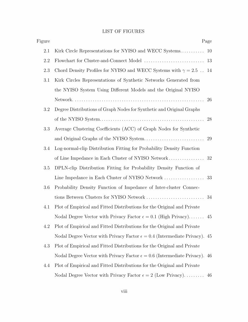
LIST OF FIGURES

Figure Page

2.1 Kirk Circle Representations for NYISO and WECC Systems. . . . . . . . . . . 10

2.2 Flowchart for Cluster-and-Connect Model . . . . . . . . . . . . . . . . . . . . . . . . . . . 13

2.3 Chord Density Profiles for NYISO and WECC Systems with γ = 2.5 . . 14

3.1 Kirk Circles Representations of Synthetic Networks Generated from

the NYISO System Using Different Models and the Original NYISO

Network. . . . . . . . . . . . . . . . . . . . . . . . . . . . . . . . . . . . . . . . . . . . . . . . . . . . . . . . . . . 26

3.2 Degree Distributions of Graph Nodes for Synthetic and Original Graphs

of the NYISO System. . . . . . . . . . . . . . . . . . . . . . . . . . . . . . . . . . . . . . . . . . . . . . . 28

3.3 Average Clustering Coefficients (ACC) of Graph Nodes for Synthetic

and Original Graphs of the NYISO System. . . . . . . . . . . . . . . . . . . . . . . . . . . 29

3.4 Log-normal-clip Distribution Fitting for Probability Density Function

of Line Impedance in Each Cluster of NYISO Network . . . . . . . . . . . . . . . . 32

3.5 DPLN-clip Distribution Fitting for Probability Density Function of

Line Impedance in Each Cluster of NYISO Network . . . . . . . . . . . . . . . . . . 33

3.6 Probability Density Function of Impedance of Inter-cluster Connec-

tions Between Clusters for NYISO Network . . . . . . . . . . . . . . . . . . . . . . . . . . 34

4.1 Plot of Empirical and Fitted Distributions for the Original and Private

Nodal Degree Vector with Privacy Factor ε = 0.1 (High Privacy). . . . . . . 45

4.2 Plot of Empirical and Fitted Distributions for the Original and Private

Nodal Degree Vector with Privacy Factor ε = 0.4 (Intermediate Privacy). 45

4.3 Plot of Empirical and Fitted Distributions for the Original and Private

Nodal Degree Vector with Privacy Factor ε = 0.6 (Intermediate Privacy). 46

4.4 Plot of Empirical and Fitted Distributions for the Original and Private

Nodal Degree Vector with Privacy Factor ε = 2 (Low Privacy). . . . . . . . . 46

viii

Figure Page

4.5 Plot of Empirical and Fitted Distributions for the Original and Private

Line Impedance Vector with Privacy Factor ε = 0.1 (High Privacy). . . . . 47

4.6 Plot of Empirical and Fitted Distributions for the Original and Private

Line Impedance Vector with Privacy Factor ε = 0.4 (Medium Privacy). 47

4.7 Plot of Empirical and Fitted Distributions for the Original and Private

Line Impedance Vector with Privacy Factor ε = 0.6 (Medium Privacy). 48

4.8 Plot of Empirical and Fitted Distributions for the Original and Private

Line Impedance Vector with Privacy Factor ε = 2 (Low Privacy). . . . . . . 48

ix

LIST OF SYMBOLS

ACC Average Clustering Coefficient of nodes in a graph

BN Boundary nodes of clusters in a graph

C Clustering coefficient

CDF Cumulative distribution function

D N -by-N distance matrix of a graph

D Truncated geometric random variable

dmax Diameter

dij The shortest path length from node i to node j

DPLN Double Pareto log-normal distribution

DPLNclip Double Pareto log-normal distribution with clipping impedance

E Edge set of a graph

E(·) Expectation of a function

Emax Local maxima of chord density profile

Emin Local minima of chord density profile

FS Sampling flag

G An undirected graph

GS A synthetic graph of G

G Non-uniform discrete random variable

GSf Global Sensitivity of function f

kavg Average degree

kmax Maximum degree

ki Nodal degree of any node i

L N -by-N Laplacian matrix of a graph

Lchar Characteristic path length

logn Log-normal distribution

lognclip Log-normal distribution with clipping impedance

x

M N -by-N adjacency matrix of a graph

m Number of edges in the graph

Mij Entry of the adjacency matrix M for node i and node j

MS Adjacency matrix of a synthetic graph

MX PGF of a random variable X

N Number of nodes in the graph

nc Number of clusters

ND Sum of random variables G and D

Ni Number of nodes in cluster i

NX Size of a random variable X

NYISO New York Independent System Operator

pi Intra-cluster degree distribution of cluster i

PDF Probability Distribution Function

PGF Probability Generating Function

PMF Probability Mass Function

qij Inter-cluster degree distribution between cluster i and j

R Radius of the Kirk circle

Rin Radius of inner circle in the Kirk circle

r Assortativity

Schord Number of chords intersecting the sweeping radius

Sfit Fitting curve for Schord

u Parameter of generalized Pareto distribution

V Node set of a graph

WECC Western Electricity Coordinating Council

zclip Impedance cutoff threshold

α Parameter of DPLN distribution

β Parameter of DPLN distribution

xi

δ Parameter of generalized Pareto distribution

ε Differential privacy parameter

η Chord angle

γ Chord density profile threshold

λ2(L) Algebraic connectivity

µ Mean value

Φ(·) Cumulative distribution function

Φc(·) Complementary cumulative distribution function

σ Standard deviation

θ Parameter of generalized Pareto distribution

xii

Chapter 1

INTRODUCTION

1.1 Background

Understanding the graphical structure of the electric power system is important

in assessing reliability, robustness, and the risk of failure of operations of this criti-

cal infrastructure network. Statistical graph models of complex networks yield much

insight into the underlying processes that are supported by the network. Such genera-

tive graph models are also capable of generating synthetic graphs representative of the

real network. This is particularly important since the smaller number of traditionally

available test systems, such as the IEEE systems, have been largely deemed to be

insufficient for supporting large simulation studies and commercial-grade algorithm

development. Thus, there is a need for statistical generative models of electric power

network that capture both topological and electrical properties of the network and

are scalable.

Electric power networks involving a collection of buses (nodes) connected by

branches (edges) naturally lend themselves to be modeled as graphs. In fact, we note

that a large-scale power network is naturally partitioned into smaller sub-networks

(clusters) because of geographical distribution, administrative, and/or political fac-

tors (such as states in the United States). However, energy sources are not uniformly

distributed geographically; this in turn translates to the presence of specific long-

haul energy transport connections between clusters. Taken together, electric power

networks are seen to exhibit topologies where local connections are highly dense and

long-range connections are relatively sparser.

In general, such local connectivity and clustering is due to the fact that a small

number of generator nodes supply power to a large number of load nodes. On the

other hand, the sparse long-range connections enable power transmission from one

1

area (cluster) to another; it has been observed that these connections are not random

in connectivity but occur between small groups of nodes in both clusters. This fact

has an intuitive explanation according to previous research [1]: long hauls require

having a right of way to deploy a long connection and it is highly likely that the long

wires will reuse part of this space. These physical and economic constraints inevitably

affect the structure of the topology.

Therefore, a good generative model for electric network graphs should capture

both topological and electrical properties of the original graph.

1.2 Research Objective

The goal of this work is to propose a model to generate synthetic graphs that

accurately captures topological and electrical properties. We seek a principled way

of generating meaningful statistically accurate synthetic graphs. The first step to-

wards this goal is to algorithmically identify and define clusters according to the

fact that local connections are highly dense and long-range connections are relatively

sparser. The cluster identification algorithm is followed by an algorithm that assigns

both intra- and inter-cluster links using empirical models obtained from the data.

Finally, impedances are assigned to the links using either the empirical distribution

of impedance or using sound statistical models.

One can make the data from the original network even more private by adding

noise to the node degree and line impedance data from the original graph using the

well-studied framework of differential privacy [2]. Following our method to generate

a synthetic graph, we also propose algorithms to differentially generate private degree

and impedance data.

1.3 Literature Review

Graph theory literature is rich with formal models for network graphs. Two

commonly used models are introduced here:

2

• Erdos-Renyi random graph model [3] in which edges are randomly chosen be-

tween nodes such that the resulting graph exhibits: (a) a small average shortest

path length; and (b) small clustering coefficient.

• Small-world model introduced by Watts and Strogatz [4] in which most nodes

are not neighbors of one another, but most nodes can be reached by a small

number of hops. These networks are characterized by: (a) small average path

length; and (b) a large clustering coefficient.

It has been noted by Wang et al. [1, 5, 6] as well as Hines et al. [7] that neither

the Erdos-Renyi random graph model [3] nor the small-world model [4] is suitable

for modeling power network graphs. This is because unlike these two models, the

average nodal degree of a power network is almost invariant to the size of the network

[1, 5]. That is, in practice large power network graphs are much sparser than what

is possible with the Erdos-Renyi random graph model [3] or the small-world model

[4]. Having placed in context the need for better graph models for electric power

networks, we now review current literature on generating synthetic power network

graphs.

Recently, Wang et al. in [1] present a stochastic generative model for electric power

networks. They introduce a Randomized Topology (RT)-nested-smallworld model [1]

which models the network as a locally dense small-world network with random long-

haul connections. Visualizing the network nodes on a ring lattice, their model (i)

creates equal-sized sub-networks (clusters) along the ring by connecting nodes within

a threshold distance of each other and rewires a small number of intra-cluster links

randomly; and (ii) determines the number of inter-cluster links between every two

neighboring sub-networks (clusters) and connects the corresponding number of nodes

in the two neighboring sub-networks (clusters) at random as inter-cluster links. This

3

model has two limitations: (a) in practice, clusters in electric power networks are not

uniform in size and connectivity density; and (b) inter-cluster connectivity cannot be

accurately modeled by random connections since these represent long-haul connec-

tions which, as mentioned before, occur between groups of nodes in both clusters.

Hines et al. in [7, 8] provide a set of metrics to evaluate graph structures and

compare the evaluation results of real electric power networks with those of net-

works generated from the Erdos-Renyi random graph model [3] and the small-world

model[4]. They claim that models developed with only topological properties are not

sufficient to generate a synthetic network for power grids, and to address this, they

quantify an electrical distance between any two nodes. The authors create a matrix

based on the proposed electrical distance and represent such electrical distances as an

unweighted graph. However, their model suffers from the limitation that the resulting

synthetic graph has a large number of isolated nodes, i.e. nodes do not connect to

any other node in the network.

Rikvold et al. in [9, 10, 11] present another generative model for electric network

graphs based on randomly connecting N nodes located in a square with a guarantee

that there is no isolated node in the network. This model is limited because it only

focuses on the averages of degree and impedance distributions, as a result of which,

the model does not capture the clustering coefficient and the locally dense clustering

behavior.

In general, large-scale electric power networks are naturally partitioned into smaller

clusters, and hence many Independent System Operators (ISOs) in the U.S. manage

their networks by partitioning them into zones. Related work on partitioning electric

power networks are briefly reviewed below.

Hines et al. develop a partitioning model [12] modeled as an optimization problem

with a multi-attribute objective function based on electrical distances, cluster sizes

4

and cluster connectedness. This model combines the K-means algorithm (i.e. a

conventional method that partitions a network into clusters and adjusts clusters until

no node is required to move between clusters) and an evolutionary algorithm to

partition an electric power network. The limitation of this model is that the number

of clusters needs to be determined in advance. If given a network without zone data,

it is hard to tell how many zones are exactly reasonable.

In [13], Ezhilarasi et al. model the network partitioning problem as an optimiza-

tion problem with the objective to minimize the maximum number of nodes within

a cluster and the connecting lines between clusters. Peiravi et al. in [14] partition

networks by calculating the eigenvector matrix of the Laplacian matrix for a given

power system and determining clusters based on the signs of components in the Feidler

vector, i.e. the second column of the eigenvector matrix.

However, these methods focus on partitioning the electric network graph for a

specific application and not to generate a synthetic graph which can be useful for

multiple applications. It is this latter that we focus on in this thesis.

1.4 Our Contributions

This thesis focuses on capturing the topological properties of electric power net-

work graph. In particular, the two limitations described above in the RT-nested-

smallworld model [1] in Section 1.3 are addressed in the model proposed in this

thesis by determining clusters (and, consequently, non-uniform cluster sizes) from the

original electric power network, and by explicitly incorporating empirical intra- and

inter-cluster degree distributions in our model. We also have observed that electrical

properties such as line impedance also exhibit differences among local and long-haul

connections and will improve our model by assigning proper line impedance.

Our contributions are two-fold:

5

• To quantify the unique topological properties of the electric graph, a new model

named Cluster-and-Connect model is proposed that identifies clusters using a

novel clustering algorithm in a graph and parametrizes the generative model

via number of clusters, number of nodes per cluster, as well as inter- and intra-

cluster degree distributions. The final synthetic graph is obtained using a graph-

creation algorithm developed at MIT [15] to generate inter- and intra-cluster

linkages between nodes using the degree distribution parameters. The steps of

generating synthetic graphs using the Cluster-and-Connect model are shown as

follows:

1. Identify and define clusters for a given network.

2. Create connections between nodes within each cluster based on the intra-

cluster degree distribution.

3. Create inter-cluster connections via the inter-cluster degree distribution

between every two clusters.

4. Find and connect isolated nodes to obtain a complete synthetic network.

• A set of metrics proposed in the literature [7, 8] is used to evaluate the synthetic

graph that our model generates; the same metrics are also used to evaluate the

graphs generated from Wang et al.’s RT-nested-smallworld model [1]. The met-

rics evaluated for the original graph will serve as a benchmark to compare our

algorithm with the existing algorithm in [1]. We advocate wide use of such stan-

dardized metrics to consistently evaluate and compare models of electric power

networks. We demonstrate that our model captures topological characteristics

of the power network such as highly dense local connectivity and clustering of

nodes that connect (sparsely) to distant nodes. The New York Independent

6

System Operator (NYISO) system is selected as the test system for generating

synthetic networks.

1.5 Outline of Thesis

The principal content of this thesis is partitioned into four chapters.

Chapter 1 presents an overview of the background, research objective, literature

review and our contributions on modeling power grids and network partitioning. In

Chapter 2, the system model and our Cluster-and-Connect model for generating syn-

thetic network graphs composed of four algorithms are described. In Chapter 3, a

set of metrics used to evaluate graphical properties is introduced. The results of

using such metrics for both the original graph and the synthetic graph generated

from the proposed approach are also presented. Chapter 4 examines how degree and

impedance distributions can be released in a private manner that satisfies differential

privacy. Chapter 5 concludes the thesis and enumerates the contributions of this

research. Possible future work in related topics is also discussed.

7

Chapter 2

SYSTEM MODEL AND CLUSTER-AND-CONNECT MODEL

This chapter introduces a novel model for generating synthetic electric power

networks, namely the Cluster-and-Connect model, to capture topological properties.

The discussion starts with the introduction of the system model and proceeds to the

Cluster-and-Connect model described as a sequence of four algorithms. The model

also concludes with a brief description of modeling the impedance distribution for the

network as an effort to model an electrical characteristic feature of the network.

2.1 System Model

Subsection 2.1.1 presents a graph representation of electric power networks. Anal-

ogous to Wang et al. [1], throughout this thesis, we use a circular graph layout, also

referred to as the Kirk circle [16], to visualize the connectivity and topology of the

electric power network graph. The description of Kirk circle is detailed in Subsection

2.1.2.

2.1.1 Graph Model for Electrical Networks

An electric power network can be represented by an undirected graph G(V ,E)

where V , the node set of the graph, consists of N nodes and E , the edge set of m

edges or links. Formally, an electric network graph consists of buses (the set V of

nodes of G) that are connected by (transmission or distribution) lines (the set E of

edges of G). A bus is either an injection or a non-injection bus, where injection implies

the existence of either a generator (power source) and/or a load (power sink) at the

bus.

For an electric power network with N nodes and m links, the number of edges

connected to any node i, i = 1, . . . , N, is defined as the nodal degree ki of that node.

The distance matrix D and the Laplacian matrix L are two other graph properties

that will be used in this paper to define features of an electric power network graph.

8

For a graph G , let dij denote the shortest path-length from node i to node j,

i.e., dij is the minimum number of edges connecting node i to node j. The distance

matrix D is then defined as

D = [dij]i=1,...,N, j=1,...,N , dii = 0, for all i. (2.1)

If there exists no path from node i to node j, then dij =∞.

The Laplacian matrix L records edge connectivity in its off-diagonal elements and

nodal degrees in its diagonal elements. The definition of the Laplacian matrix L is

L(i, j) =

−1, if dij = 1,

ki, for i = j,

0, otherwise.

(2.2)

Finally, the connectivity of nodes in a graph is captured by an N ×N adjacency

matrix M with non-zero unit entries Mij if and only if node i is connected to node j.

2.1.2 Kirk Circle

The Kirk circle [16] is a tool to visualize graph topologies used in [1] to compare

different graph models for electric power networks and is similar to the circular layout

graph drawing algorithm [17]. In general, nodes (buses) in an electric power network

are numbered with neighboring nodes assigned consecutive or closely proximal num-

bers. This allows one to sequentially map these nodes in increasing order of their

numerical labels to evenly spread points on a circle. The edge connections (branches)

between nodes are indicated by straight lines (chords) between the appropriate points

on the circle. In electric power networks, proximal and closely connected nodes indi-

cate either geographical proximity or dependence on specific subsets of generators.

Figs. 2.1a-2.1b show two representative network topologies, using Kirk circle

graphs, of the NYISO and the Western Electricity Coordinating Council (WECC)

9

systems respectively. Irrespective of size, both networks reveal a pattern of multiple

clusters (identified with the algorithms detailed in Chapter 2) with dense intra-cluster

connections and relatively sparser inter-cluster connections between clusters. Note

that colors of intra-cluster connections within clusters 1-6 for both NYISO and WECC

systems are cyan, red, green, yellow, pink and blue, respectively. Colors of inter-

cluster links are gray. Boundary points for clusters are labeled A, B, C, D, E, F.

Cl. 1

Cl. 2Cl. 3

Cl. 4

Cl. 5Cl. 6

A

B

C

D

E

F

(a) NYISO System

Cl. 1Cl. 2

Cl. 3

Cl. 4

Cl. 5

Cl. 6

A

B

C

D

EF

(b) WECC System

Figure 2.1: Kirk Circle Representations for NYISO and WECC Systems.

10

2.2 Cluster-And-Connect Model

The Cluster-and-Connect model is described as a sequence of four algorithms. As

the first step to describing our algorithms, we formally define two quantities used in

clustering and list all parameters of the network that we identify. Recall that the

number of nodes in the graph is N and the edges are represented by chords in the

Kirk circles.

Definition The chord density profile is obtained by sweeping the Kirk circle of an

arbitrary radius, R, in angular steps of (360/N) degree, such that at (360/N) degree,

the chord density is the ratio of the number of chords intersecting the radius to the

total number of chords.

Definition A cluster is a slice (arc) of the Kirk circle whose boundary points are

those at which the chord density profile has local minima satisfying a certain threshold

γ.

We identify the following four parameters to generate synthetic electric network

graphs.

1. Number of clusters (nc)

2. Number of nodes in each cluster (Ni, i = 1 . . . nc)

3. Intra-cluster degree distribution (pi, i = 1 . . . nc)

4. Pairwise inter-cluster degree distribution (qij, i, j = 1, 2, . . . , nc, i 6= j)

Figure 2.2 presents a flowchart of our algorithmic approach to generate a synthetic

graph from a given graph. The two broad steps are: (i) determine clusters; and (ii)

generate the synthetic graph. Once the clusters are identified, the synthetic graph

11

is generated in three steps: (i) generating intra-cluster connections; (ii) generating

inter-cluster connections; and (iii) eliminating isolated nodes.

We use inter- and intra-cluster degree distributions, pi and qij, respectively, to

generate a synthetic graph. Degree distributions can be generated using either sta-

tistical models (e.g., [1]) or by determining the empirical distribution from the real

graphs and then sampling from them. In this paper, we use the latter approach. For

evaluation purposes, we also use the original graph’s parameters directly. To this end,

we introduce a sampling flag FS to indicate whether the original or sampled degree

sequences will be used in the generating algorithms. Finally, we note that the inputs

nc and the Ni’s to Algorithms 2-4 are obtained from Algorithm 1. We now briefly

describe Algorithms 1-4.

2.2.1 Cluster Identification

Our clustering algorithm captures the graphical observation that there appears to

be boundary points on the Kirk circle (e.g., see points A, B, C, D, E and F in Figs. 2.1a

and 2.1b) such that nodes within these boundary points are more densely connected

amongst themselves than to those outside. We seek to detect these boundary points,

and thereby, identify clusters. While some nodes on the Kirk Circle may be well

connected to relatively distant (on the circle) nodes (e.g. nodes in clusters 5 and 6 in

Fig. 2.1a), we use the fact that consecutively numbered nodes are physically adjacent

to determine the clusters they belong to.

As the first step to determining cluster boundaries, we eliminate the inter-cluster

connections in Algorithm 1. To this end, we introduce an inner circle of radius

Rin = ηR where η is defined as a fraction of the Kirk circle radius, such that all

chords that cross the inner circle do not contribute to the chord density count. The

chord angle η determines the maximal angle that a chord subtends at the center of

the circle, and a smaller η allows us to include larger angles and vice versa. The

12

Identify Clusters

(Algo. 1)

Create Intra-cluster Node Links

(Algo. 2)

Create Inter-cluster Node Links

(Algo. 3)

Reconnect Isolated Nodes

(Algo. 4)Genera

te S

yn

theti

c G

raph

s

Original Graph G,

Sampling Flag FS

Synthetic Graph GS

FS = 1?Original Degree

Sequence

Sampled Degree

Sequence

NY

Relocate isolated nodes within clusters

Figure 2.2: Flowchart for Cluster-and-Connect Model

subplots 2.3a and 2.3b in Fig. 2.3 show the corresponding smoothed chord density

profiles for the NYISO and WECC data, respectively.

Note that there are a number of local minima and maxima in subplots 2.3a and

2.3b in Fig. 2.3. To identify clusters of sufficient size (and acknowledge the fact that

within a cluster a subset of nodes may be more connected than others), we use a

threshold parameter γ to determine the cluster boundaries, and therefore, the total

number of clusters. Without loss of generality, we assume we begin at a minimum.

13

0 5 0 1 0 0 1 5 0 2 0 0 2 5 0 3 0 0 3 5 00 . 0 0

0 . 0 2

0 . 0 4

Coun

t

A n g l e ( D e g r e e )

F i t t i n g L o c a l M i n i m a L o c a l M a x i m a D i v i d i n g N o d e s

A B C D EF

(a) NYISO with Boundary Nodes {A,B,C,D,E,F}={1,112,739,1295,1652,2331}

0 5 0 1 0 0 1 5 0 2 0 0 2 5 0 3 0 0 3 5 00 . 0 0

0 . 0 4

0 . 0 8 F i t t i n g L o c a l M i n i m a L o c a l M a x i m a B o u n d a r y N o d e s

Coun

t

A n g l e ( D e g r e e )

A B C D E F

(b) WECC with Boundary Nodes {A,B,C,D,E,F}={1,1031,2203,2410,3278,3756}

Figure 2.3: Chord Density Profiles for NYISO and WECC Systems with γ = 2.5

Then, at the kth local minimum, we compute two ratios: one using the immediate

maximum to the left of this minimum Emax[k − 1]/Emin[k] and the other using the

immediate maximum to its right Emax[k]/Emin[k]. If any of the two ratios is larger

than γ, the local minimum is determined to be a boundary point. Thus, the choice of

γ determines the number of clusters nc and the corresponding cluster sizes Ni. Finally,

we check the nodal degrees of nodes within each cluster for intra-cluster connections.

If any isolated node does not connect to any other neighboring node within the same

cluster that means its nodal degree is zero, it will move to the immediately connecting

14

node in another cluster. If more than one node is connected to the isolated node, we

will choose the connecting node where the line impedance between these two nodes

is smaller.

Algorithm 1 Identifying Clusters

Inputs: η, γ, and the Laplacian matrix L for a given graph G.

Outputs: nc, Ni for all i = 1, ..., nc.

1. Draw a Kirk circle with an arbitrary radius R based on L for a given graph G.

2. Draw an inner circle with a radius Rin = ηR. Ignore links that pass through

the inner circle.

3. Obtain the number of nodes N as the number of rows (or columns) of L. Sweep

the Kirk circle in steps of (360/N)◦ from the first node in a counter-clock fashion.

Keep count of the number of chords that intersect the sweeping radius as a vector

Schord.

4. Fit a curve Sfit for the points in Schord.

5. Find local maxima Emax[1 : K−1] and local minima Emin[1 : K] for fitted curve

Sfit.

6. For k = 2, ..., K − 1, calculate ratios Rprev[k − 1] = Emax[k − 1]/Emin[k] and

Rnext[k − 1] = Emax[k]/Emin[k] with its two adjacent maxima.

7. Set first boundary node BN [1] = Emin[1] = 1. For k = 2, ..., K − 1, if eithor

Rprev[k − 1] or Rnext[k − 1] > γ, record Emin[k] as a boundary node.

8. Obtain the set of boundary nodes BN [1 : nc].

15

2.2.2 Generating Synthetic Graphs

Using the clusters identified above, Algorithms 2 and 3 generate inter- and intra-

cluster linkages, respectively. To do so, we use the software package MIT Matlab tools

for network analysis offered by the Strategic Engineering Research Group of MIT

[15]. In particular, we use the program graph from degree sequence.m which does the

following: it orders the input degree sequence in descending order and connects nodes

with the highest adjacent degrees iteratively until all degrees are assigned. It is worth

noting that the graph obtained using the deterministic MIT algorithm [15] will in

general be different from the original graph.

At the outset, Algorithm 2 creates a degree sequence realization DSi[1 : Ni] which

is obtained by sampling pi for cluster i if FS = 1 or is set to the degree sequence of

the original graph if FS = 0. This is then used to generate intra-cluster connections

using the MIT toolbox [15].

Following Algorithm 2, we create inter-cluster connections using Algorithm 3.

This algorithm requires two degree sequences as inputs: DOij of outgoing edges from

cluster i to cluster j obtained from qij and DOji of outgoing edges from cluster j to

cluster i obtained from qji. If FS = 1, DOij and DOji are sampled from qij and qji,

respectively; otherwise, they are computed from the original graph. Since two degree

sequences are involved, we tailor the graph from degree sequence.m program to create

connections using degree sequences from two clusters; we do so in a similar fashion

to the original algorithm by ordering both sequences in descending order of degrees.

The detailed steps of Algorithms 2 and 3 are listed below.

16

Algorithm 2 Intra-cluster Node Linkage

Inputs: nc, Ni, pi for all i = 1, ..., nc, and FS.

Output: Adjacency matrix MS for synthetic graph GS.

1. Start from cluster i = 1. If FS = 1, generate a sample degree sequence DSi[1 :

Ni] from pi, otherwise make DSi[1 : Ni] = pi.

2. If∑

kDSi[k] is odd, add one degree to DSi[1].

3. Reorder DSi[1 : Ni] in descending order as DSi[1 : Ni] with reordered node

indices Indi[1 : Ni].

4. If DSi[1] = 0, exit loop. Else, start with DSi[1].

5. Create links from Indi[1] to Indi[2], Indi[3], ..., Indi[DSi[1] + 1] by updating

corresponding entries of MS.

6. Subtract 1 from DSi[2 : DSi[1] + 1] and set DSi[1] = 0.

7. Repeat Steps 3-6 until DSi[1] = 0 in Step 4.

8. Repeat Steps 1-7 for i = 2, ...nc.

17

Algorithm 3 Inter-cluster Node Linkage

Inputs: nc, Ni, qij for all i, j = 1, ..., nc, i 6= j and FS.

Output: Updated adjacency matrix MS for synthetic graph GS.

1. Start from cluster i = 1, j = i + 1. First, if FS = 1, generate an out-going

degree sequence DOij[1 : Nj] by sampling qij. Then generate out-going degree

sequence DOji[1 : Ni] from qji, stopping when∑DOij[1 : Ni] =

∑DOji[1 : Nj].

If FS = 0, DOij[1 : Nj] = qij and DOji[1 : Ni] = qji.

2. Reorder DOij[1 : Ni] and DOji[1 : Nj] in descending order as DOij[1 : Ni]

and DOji[1 : Nj] with reordered node indices Indij[1 : Ni] and Indji[1 : Nj],

respectively.

3. Start with DOij[k = 1].

4. Create links from Indij[k] to Indji[1], Indji[2], ..., Indji[DOij[k]] by updating

MS.

5. Subtract 1 from DOji[1 : DOij[k]].

6. Reorder DOji[1 : Nj] in descending order as DOji[1 : Nj] with reordered node

index Indji[1 : Nj].

7. Repeat Step 3-6 for k = 2, ..., Ni.

8. Repeat Steps 1-7 for j = i+ 2, ...., nc, j 6= i.

9. Repeat Steps 1-8 for i = 2, ..., nc.

18

Finally, unlike an actual electric network graph, a synthetic graph generated from

degree distributions may have islands (i.e., the nodes whose distance matrix entries

relative to each other are non-infinite but no node in the island has finite distance

relative to any node outside this island). After generating intra- and inter-cluster

connections, Algorithm 4 checks for islands using the distance matrix D and resolves

them by rewiring or adding links.

Algorithm 4 Reconnecting Islands

Input: Adjacency matrix MS of synthetic graph GS.

Output: Final adjacency matrix of GS.

1. Identify the islands using the distance matrix D (those elements with dij =∞).

2. Determine the vector of degrees of the nodes in the islands Degc[:] and sort it

in descending order as Degc[:] and the sorted node index as IndDeg[:].

3. Identify a link outside the island with end nodes ol and ok.

4. If Degc[1] is connected to some node j within the island with degree > 2,

then replace this link with two links from IndDeg[1] and IndDeg[j] to ol and ok,

respectively. Update MS. Go to Step 6.

5. Else, introduce a new link from Degc[1] to node o` and update MS.

6. End.

2.2.3 Line Impedance Assignment

A complete model of generating synthetic networks should not only limit to

the properties of topology but should also focus on the electrical properties. Line

impedance is considered to be one of the most important properties that represents

19

the weight of each line as well as the geographical distance between every two nodes

(in general, the line impedance is proportional to the physical distance for each line).

From the observations obtained by Wang et al. [5], they conclude that the dis-

tribution of line impedance of power grids is heavily tailed according to the empiri-

cal histogram Probability Distribution Function (PDF). Two candidate distribution

functions, the log-normal distribution and the double Pareto log-normal (DPLN) dis-

tribution, can be used for fitting the NYISO data. These two distributions are defined

below.

Given the original data x,

Log-normal:

logn(x|µ, σ) =1

xσ√

2πexp(−(lnx− µ)2

2σ2) (2.3)

where µ and σ are the mean and standard deviation;

Double Pareto log-normal:

DPLN(x|α, β, µ, σ) =αβ

α + β[A(α, µ, σ)x−α−1Φ(

lnx− µ− ασ2

σ)

+A(−β, µ, σ)xβ−1Φc(lnx− µ+ βσ2

σ)]

(2.4)

where A(θ, µ, σ) = exp(θµ+ θ2σ2/2). Φ and Φc are cumulative distribution function

and complementary cumulative distribution function, respectively. α and −β (α > 0,

β > 0) are the two roots of the quadratic equationσ2

2z2 + (µ− σ2

2)z − λ = 0, where

λ is a constant rate.

Wang et al. in [1] observes that the original impedance data may have an inter-

rupted tail which can be captured by the clipping. To do so, the impedance data

are clipped with exponential cutoff. The log-normal and double Pareto log-normal

(DPLN) are modified to the log-normal-clip and DPLN-clip distributions.

Given the original data x, the clipped impedance data is [1]:

zclip(1− exp(− x

zclip

)) (2.5)

20

where zclip is the impedance cutoff threshold.

The log-normal-clip and DPLN-clip distributions are formally defined as follows.

Log-normal-clip:

lognclip(x|µ, σ, zclip) =zclip

zclip − x× logn(−zclip × ln(1− x

zclip

)|µ, σ) (2.6)

DPLN-clip:

DPLNclip(x|α, β, µ, σ, zclip) =zclip

zclip − x×DPLN(−zclip × ln(1− x

zclip

)|α, β, µ, σ) (2.7)

Note that the fitting parameters of both log-normal-clip and DPLN-clip distribu-

tions are estimated from the original impedance distribution following the maximum

likelihood criterion mentioned in [1], and are guaranteed for the best fitting distribu-

tion by an appropriately modified Kolmogorov-Smirnov test (K-S test).

21

Chapter 3

EVALUATION METRICS AND SIMULATION RESULTS

In this chapter, we first introduce a set of metrics to evaluate graphs. These met-

rics mainly focus on topological properties and are applied to evaluate the synthetic

graphs generated from the Cluster-and-Connect model. As shown by Wang et al. in

[1], line impedance can be statistically modeled by specific well-studied heavy-tailed

distributions, e.g., log-normal-clip and double Pareto log-normal-clip (DPLN-clip) as

verified by us earlier in Section 2.2.3. We use these distributions, as appropriate,

to model the distribution of intra-cluster line impedances; for the inter-cluster case,

due to the sparse connections, we sample directly from the empirical distribution as

detailed in this chapter.

3.1 Topological Evaluation Metrics

The topological properties of a graph can be quantified by a set of measures that

capture connectivity and distance properties between nodes formally. These mea-

sures, including maximum degree, average degree, clustering coefficient, and related

quantities, are presented in the context of electric power network graphs by Cotilla-

Sanchez et al. in [7]. Analogous to [7], we define and identify the following measures

that will be applied to evaluate graph generation models below. Recall that N is the

number of nodes and m is the number of edges in the graph G.

• Maximum degree kmax: the maximal nodal degree among all the nodes,

kmax = maxiki, i = 1, ..., N. (3.1)

• Average degree kavg: the mean of the nodal degrees for all the nodes,

kavg =

∑Ni=1 kiN

. (3.2)

22

• Diameter dmax: the maximal shortest path length in the network, i.e., for dij in

(2.1), dmax is given by

dmax = maxij

dij, i, j = 1, ..., N, i 6= j. (3.3)

• The characteristic path length Lchar: the mean of all shortest path lengths

traversing from one node to the other,

Lchar =

∑∀i,j i6=j dij

N(N − 1). (3.4)

• The clustering coefficient C of a graph G is the average value of the node clus-

tering coefficient ci over all nodes i = 1, 2, ..., N , that quantifies the extent to

which nodes in a graph tend to locate nearby and connect to each other given

by

C =

∑Ni=1 ciN

, (3.5)

where ci denotes the fraction of the actual existing links ϕ(i) among the nodes

connected to node i over all the possible links (complete graph) that can exist

among these nodes as,

ci =2ϕ(i)

ki(ki − 1). (3.6)

• Assortativity r: quantifies the extent to which nodes connect to nodes with

similar degrees. Formally, it is the correlation in degree for the nodes on opposite

ends of each link

r =m−1

∑mi=1 aibi − [m−1

∑mi=1

12(ai + bi)]

2

m−1∑m

i=112(a2i + b2

i )− [m−1∑m

i=112(ai + bi)]2

, (3.7)

where ai and bi are the degrees of the endpoints of link i.

• Algebraic connectivity λ2(L)[18]: is the second smallest eigenvalue of the Lapla-

cian matrix L reflecting how well a network is connected. If the λ2(L) is close

23

to 0, the network is close to being disconnected; if λ2(L)/N is close to 1, the

network is close to being fully connected.

3.2 Simulation Results

In this section, we use the metrics introduced in Section 3.1 to evaluate the ac-

curacy of the synthetic graphs generated from our Cluster-and-Connect model for

the NYISO system; we also use the same metrics to evaluate the synthetic graph

generated using the RT-nested-smallworld model proposed in [1] and compare it with

those for our model. The metrics for the original graph are used as a benchmark to

evaluate both algorithms.

The test system is the NYISO system, which has 2935 nodes and 7028 edges. We

use the Cluster-and-Connect algorithm to generate two synthetic graphs: (i) synthetic

graph SG1 generated using sampled degree sequences; and (ii) synthetic graph SG2

generated using original degree sequences. Observe that if the sampling flag Fs = 1,

it means the graph SG1 is generated with the sampled degree sequences from pi and

qij respectively for intra- and inter-cluster connections; if setting FS = 0, the intra-

and inter-cluster degree sequences are obtained directly from the original graph and

SG2 is generated. We remark that SG2 shares the same degree distribution as the

original graph. However, as mentioned earlier, the intra- and inter- connections of

SG2 are different from the original graph as a result of using the MIT Toolbox [15]

in Algorithms 2 and 3 (see Fig. 2.2). Wang et al.’s algorithm [1] is also utilized to

generate a RT-nested-smallworld graph SGRTSW with 3000 nodes.

We now compare the original NYISO graph with SG1 and SG2, both visually

using the Kirk circle and the metrics introduced in Section 3.1. In Fig. 3.1, subplots

3.1a-3.1d correspond to the Kirk circle representations of SG1, SG2, SGRTSW , and

the original NYISO system, respectively.

24

(a) Cluster-and-Connect: SG1, Sampled Degree Sequence

(b) Cluster-and-Connect: SG2, Original Degree Sequence

25

(c) RT-nested-smallworld: SGRTSW

(d) the NYISO System

Figure 3.1: Kirk Circles Representations of Synthetic Networks Generated from theNYISO System Using Different Models and the Original NYISO Network.

26

Table 3.1: Metrics for Different Graphs Based on the NYISO System

Metrics NYISO

Cluster-and-

Connect (i):

SG1, sampled

Cluster-and-

Connect (ii):

SG2, original

RT-nested-

smallworld:

SGRTSW

Nodes 2935 2935 2935 3000

Links 7028 7066 7177 7082.66

kmax 38 38 38 20.63

kavg 4.7891 4.8150 4.8497 4.7218

dmax 54 33 39 40.83

Lchar 18.4209 11.6786 11.9361 18.5481

C 0.2096 0.2648 0.2626 0.1791

r 0.4487 0.7372 0.7452 -0.1027

λ2(L) 0.0015 0.0026 0.0024 0.0012

As seen from the Kirk circles in Figs. 3.1a-3.1d, our synthetic graphs SG1 and

SG2 generated from Cluster-and-Connect model appears to capture the inter-node

connections more accurately than the synthetic graph generated from RT-nested-

smallworld model for the NYISO system. We quantify our evaluation metrics for all

four graphs in Table 3.1. Note that, since the process for generating SG1 is stochastic,

we generate a hundred synthetic graphs and report the average of various graph

statistics. For SG2, there is only one synthetic graph because the degree sequence is

deterministic.

We briefly discuss the results in Table 3.1.

27

• Nodes : Our model keeps the same number of nodes as in the NYISO system.

Wang et al.’s model [1] approximates this number because of the uniform size

of clusters.

• Links : The number of links in synthetic graphs SG1 and SG2 are often larger

than those in the original NYISO graph. The additional links are added in

Algorithm 4 because of isolated nodes generated in Algorithm 2.

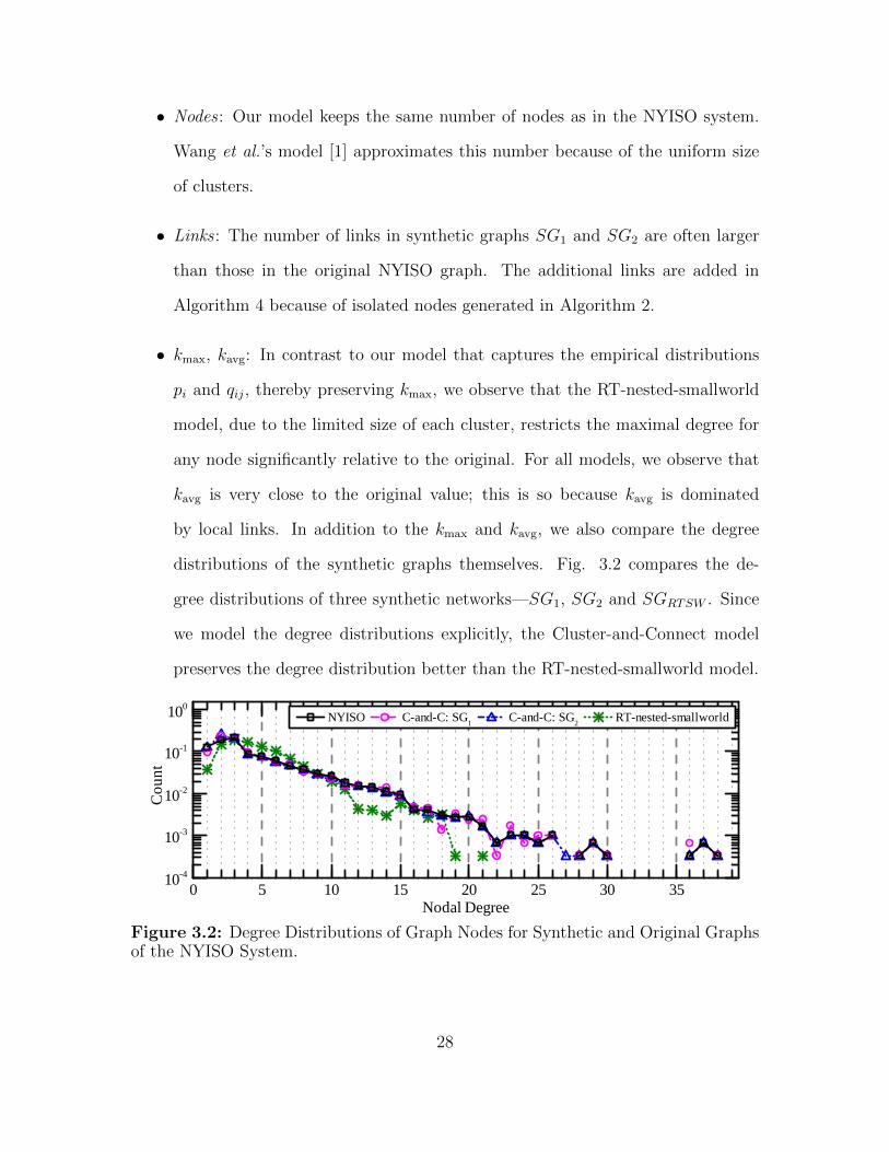
• kmax, kavg: In contrast to our model that captures the empirical distributions

pi and qij, thereby preserving kmax, we observe that the RT-nested-smallworld

model, due to the limited size of each cluster, restricts the maximal degree for

any node significantly relative to the original. For all models, we observe that

kavg is very close to the original value; this is so because kavg is dominated

by local links. In addition to the kmax and kavg, we also compare the degree

distributions of the synthetic graphs themselves. Fig. 3.2 compares the de-

gree distributions of three synthetic networks—SG1, SG2 and SGRTSW . Since

we model the degree distributions explicitly, the Cluster-and-Connect model

preserves the degree distribution better than the RT-nested-smallworld model.

0 5 1 0 1 5 2 0 2 5 3 0 3 51 0 - 4

1 0 - 3

1 0 - 2

1 0 - 1

1 0 0

Coun

t

N o d a l D e g r e e

N Y I S O C - a n d - C : S G 1 C - a n d - C : S G 2 R T - n e s t e d - s m a l l w o r l d

Figure 3.2: Degree Distributions of Graph Nodes for Synthetic and Original Graphsof the NYISO System.

28

• dmax, Lchar: We observe that dmax and Lchar of synthetic graphs SG1 and SG2

generated from our Cluster-and-Connect algorithm are lower compared to the

original graph. This is due in part to the limitation of Algorithm 2 in modeling

the intra-cluster links; it appears these links are locally dense within clusters

which our model does not capture accurately. The restricted neighborhood

model of RT-nested-smallworld appears to capture this, however, at the cost of

other metrics kmax, C and r.

• C: Since we reconnect isolated nodes in Algorithm 4 by adding extra links,

the resulting clustering coefficients C of our synthetic graphs SG1 and SG2 are

higher than that of the original NYISO graph. Nevertheless, from Fig. 3.3—

which compares the average clustering coefficients (ACC) of graph nodes of

a particular degree (rather than the clustering coefficient of the entire graph)

of the three synthetic networks—we see that our model preserves the average

clustering coefficient of graph nodes far better than the RT-nested-smallworld

model.

0 5 1 0 1 5 2 0 2 5 3 0 3 51 0 - 1

1 0 0 N Y I S O C - a n d - C : S G 1 C - a n d - C : S G 2 R T - n e s t e d - s m a l l w o r l d

ACC

N o d a l D e g r e eFigure 3.3: Average Clustering Coefficients (ACC) of Graph Nodes for Syntheticand Original Graphs of the NYISO System.

• r and λ2(L): The assortativity r captures the extent to which nodes of similar

degrees are connected to each other; the restricted neighborhood model of RT-

29

nested-smallworld leads to a very small, in fact, negative, r which indicates that

connected nodes have largely different degrees. On the other hand, our model

captures but overcompensates due to the preferential connectivity of similar

degree nodes in Algorithm 2. One observes a similar behavior with λ2(L).

Recall that in Subsection 2.2.3, Wang et al. in [1] conclude that both the log-

normal-clip and double Pareto log-normal-clip (DPLN-clip) distributions fit for the

impedance data of the NYISO system. In addition to the results of fitting impedance

data for the entire network shown in [1], we apply the two distributions on the

impedance data of each cluster respectively to get impedance data estimated for the

intra-cluster connections. The impedance of inter-clusters connections between two

clusters are assigned directly by sampling from the original impedance data because

the inter-cluster connections are so sparse.

The fitting parameters of the log-normal-clip and DPLN-clip distributions for each

cluster of the NYISO system are listed in Table 3.2 and Table 3.3, respectively. The

probability density function of the log-normal-clip and DPLN-clip distributions are

shown in Fig. 3.4 and Fig. 3.5 respectively, including the original impedance distri-

bution and the fitting distribution. Note that, each subplot shows the distributions

for one cluster.

We briefly discuss the results in Fig. 3.4 and Fig. 3.5. It is clear that both log-

normal-clip distribution and DPLN-clip distribution fit well on the line impedance

data for intra-cluster connections. However, in some clusters, e.g. cluster 2 in Figs.

3.4 and 3.5, there shows a peak in the middle of the fitting curves which represents

the deviation from the original impedance data for the small impedances. The im-

provement of the fitting distributions for the impedance data, in particular for the

small impedances, can be our future work.

30

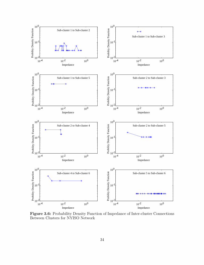
Fig. 3.6 shows the probability density function of the impedance of inter-cluster

connections between clusters. From the distribution, one can observe that the inter-

cluster connections are very sparse. In our model, we sample impedance of inter-

cluster connections directly from the empirical impedance distribution.

Table 3.2: Parameters of Log-normal-clip Distribution Fitting for Probability Dis-tribution Functions of Line Impedance

Cluster Number µ σ zclip

1 -3.9598 2.2580 1.9773

2 -2.9299 1.4930 1.9008

3 -2.8271 1.8279 2.4633

4 -3.2525 1.9771 2.4595

5 -2.9910 1.7404 2.6024

6 -1.1771 1.9197 3.6503

Table 3.3: Parameters of DPLN-clip Distribution Fitting for Probability Distribu-tion Functions of Line Impedance

Cluster Number α β µ σ zclip

1 44.0000 44.0000 -3.9598 2.2578 1.9773

2 45.0000 44.0000 -2.9294 1.4926 1.9008

3 44.0000 45.0000 -2.8276 1.8276 2.4633

4 45.0000 45.0000 -3.2525 1.9769 2.4595

5 44.0000 45.0000 -2.9915 1.7401 2.6024

6 45.0000 44.0000 -1.1766 1.9194 3.6503

31

10-4

10-2

100

102

10-5

100

Impedance

Pro

babi

lity

Den

sity

Fun

ctio

n

Cluster 1

OriginalLog-normal Fitted

10-4

10-2

100

102

10-5

100

Impedance

Pro

babi

lity

Den

sity

Fun

ctio

n

Cluster 2

OriginalLog-normal Fitted

10-4

10-2

100

102

10-5

100

Impedance

Pro

babi

lity

Den

sity

Fun

ctio

n

Cluster 3

OriginalLog-normal Fitted

10-4

10-2

100

102

10-5

100

Impedance

Pro

babi

lity

Den

sity

Fun

ctio

n

Cluster 4

OriginalLog-normal Fitted

10-4

10-2

100

102

10-5

100

Impedance

Pro

babi

lity

Den

sity

Fun

ctio

n

Cluster 5

OriginalLog-normal Fitted

10-4

10-2

100

102

10-5

100

Impedance

Pro

babi

lity

Den

sity

Fun

ctio

n

Cluster 6

OriginalLog-normal Fitted

Figure 3.4: Log-normal-clip Distribution Fitting for Probability Density Functionof Line Impedance in Each Cluster of NYISO Network

32

10-4

10-2

100

102

10-8

10-6

10-4

10-2

100

Impedance

Pro

babi

lity

Den

sity

Fun

ctio

n

Cluster 1

OriginalDPLN Fitted

10-4

10-2

100

102

10-8

10-6

10-4

10-2

100

Impedance

Pro

babi

lity

Den

sity

Fun

ctio

n

Cluster 2

OriginalDPLN Fitted

10-4

10-2

100

102

10-8

10-6

10-4

10-2

100

Impedance

Pro

babi

lity

Den

sity

Fun

ctio

n

Cluster 3

OriginalDPLN Fitted

10-4

10-2

100

102

10-8

10-6

10-4

10-2

100

Impedance

Pro

babi

lity

Den

sity

Fun

ctio

n

Cluster 4

OriginalDPLN Fitted

10-4

10-2

100

102

10-8

10-6

10-4

10-2

100

Impedance

Pro

babi

lity

Den

sity

Fun

ctio

n

Cluster 5

OriginalDPLN Fitted

10-4

10-2

100

102

10-8

10-6

10-4

10-2

100

Impedance

Pro

babi

lity

Den

sity

Fun

ctio

n

Cluster 6

OriginalDPLN Fitted

Figure 3.5: DPLN-clip Distribution Fitting for Probability Density Function of LineImpedance in Each Cluster of NYISO Network

33

10-4 10-2 10010-2

10-1

100

Impedance

Prob

ility

Den

sity

Fun

ctio

n Sub-cluster 1 to Sub-cluster 2

10-4 10-2 10010-2

10-1

100

Impedance

Sub-cluster 1 to Sub-cluster 3

10-4 10-2 10010-2

10-1

100

Impedance

Sub-cluster 1 to Sub-cluster 5

10-4 10-2 10010-2

10-1

100

Impedance

Sub-cluster 2 to Sub-cluster 3

10-4 10-2 10010-2

10-1

100

Impedance

Sub-cluster 2 to Sub-cluster 4

10-4 10-2 10010-2

10-1

100

Impedance

Sub-cluster 2 to Sub-cluster 5

10-4 10-2 10010-2

10-1

100

Impedance

Sub-cluster 4 to Sub-cluster 6

10-4 10-2 10010-2

10-1

100

Impedance

Sub-cluster 5 to Sub-cluster 6

Prob

ility

Den

sity

Fun

ctio

n

Prob

ility

Den

sity

Fun

ctio

n

Prob

ility

Den

sity

Fun

ctio

n

Prob

ility

Den

sity

Fun

ctio

n

Prob

ility

Den

sity

Fun

ctio

n

Prob

ility

Den

sity

Fun

ctio

n

Prob

ility

Den

sity

Fun

ctio

n

Figure 3.6: Probability Density Function of Impedance of Inter-cluster ConnectionsBetween Clusters for NYISO Network

34

Chapter 4

DIFFERENTIAL PRIVACY

In this chapter, we consider the problem of generating privacy-assured degree and

impedance distributions. This involves adding noise in a judicious manner to degree

and impedance sequences obtained from the original graph. Iteratively, one could

also generate realizations of degree and impedance sequences from their empirical

distributions and add noise intelligently to preserve a desired measure of privacy. To

this end, we first consider statistical models for degree and impedance data of an

electric power network graph. In [1], Wang et al. introduce statistical models for the

two distributions and we first overview their model in Section 4.1.

4.1 Model for Nodal Degree Distribution and Impedance Distribution

We use statistical models, introduced by Wang et al. in [1], that are designed to

fit the degree and impedance data. Comparing the empirical and fitted distribution

with and without differential privacy provides a meaningful method to compare the

effect of privacy on the distribution of nodal degree and line impedance.

4.1.1 Nodal Degree Distribution

It has been observed that the nodal degree distribution of electric networks dis-

plays an exponential tail, i.e., a simple model for the nodal degree could be p(ki) =

exp(−ki/kavg)/kavg where p (ki) is the probability mass function (PMF) of node i

having a degree ki. However, in [1], using real-world power grid data, the authors

show that while a geometric distribution fits well for the tail distribution (of nodal

degrees), for the range of small node degrees, that is ki ≤ 3, the empirical PMF

deviates from such a model and in fact requires modeling the degree distribution as

resulting from a random variable ND that is the sum of two random variables G and

D, where G and D are non-uniform discrete and truncated (due to the finite degree

bound) geometric random variables, respectively. Thus, we have

35

ND = G+D (4.1)

where G is a truncated geometric with parameter p and truncation length of kmax

such that

Pr (G = k) =(1− p)k p∑kmax

k=0 (1− p)k p(4.2)

=(1− p)k p

1− (1− p)kmax+1, k = 0, 1, 2, ..., kmax, (4.3)

and D is a discrete random variable with probabilities {p1, p2, ..., pkt} such that

Pr (D = k) = pk, k = 1, 2, ..., kt. (4.4)

The nodal degree then has a distribution given by the convolution of G and D, i.e.,

Pr (ND = k) = Pr (G = k) ⊗ Pr (D = k) , k = 0, 1, 2..., kt + kmax − 1. To estimate

the parameters of the two component distributions of ND, and therefore, that of ND

itself, one can use the probability generating function (PGF) where the PGF of a

random variable X is defined as MX (z) =∑

k Pr (X = k) zk. Furthermore for sum of

independent random variables, the PGF of ND is given as MND(z) = MG (z)MD (z) .

One can estimate the PGF of a random variables X from an observed (sample

set) data set of size NX using the fact that the expected value of the function zX ,

where the expectation is over X, can be obtained by taking the average of zX over

all feasible values of X [1]. Thus, for a given sample data set X of size NX , the PGF

of X can be estimated from the mean of zX as

E(zX)

=∑k

n(X=k)

NX

zk (4.5)

≈∑k

Pr (X = k) zk, (4.6)

36

where n(X=k) denotes the total number of data items that take the value k. For very

large N , the ‘type count’ n(X=k)/N approaches Pr (X = k) allowing the approxima-

tion in (4.6). For the distributions modeled in (4.3) and (4.4), one can show that the

PGF of ND is

MND(z) =

p(

1− ((1− p) z)kmax+1)∑kt

i=1 pizi(

1− (1− p)kmax+1)

(1− (1− p) z). (4.7)

Thus, MNDhas kmax zeros evenly distributed on a circle of radius 1/ (1− p) from

the truncated geometric and kt zeros from the discrete distribution. The approxi-

mation in (4.6) is then used to obtain contour plots of the PGF to determine the

zeros of MND(z) and therefore effectively the parameters p, kt, and kmax as well as

the starting values for the discrete distribution probabilities {pi}ktt=1 . We illustrate

the use of such contour plots to obtain these parameters and compute a distribution

fitting the empirical nodal degree distribution in the following section.

4.1.2 Line Impedance Distribution

Wang et al. propose a variety of heavy-tailed distributions in [1] such as Gamma,

Generalized Pareto, log-normal, and double Pareto log-normal as statistical models

for impedance distributions of several electric power networks, e.g., IEEE bus systems

and the NYISO system. We use the IEEE 300 bus system for line impedance data

in our simulation. The fitting model proposed for this in [1] is a generalized Pareto

distribution with parameters u, δ, and θ given by

GP (x|u, δ, θ) =

(1

δ

)(1 + u

(x− θ)δ

)−1−(1/u)

. (4.8)

The data from the 300 bus system will be used to estimate these parameters for

both the cases with and without the application of a differentially private mechanism.

In the following section we detail the privacy mechanism we use for both node

and edge privacy in graphs.

37

4.2 Differential Privacy for Graphs

In this section, we introduce the notion of differential privacy. Next, we outline our

algorithms for generating differentially private synthetic degree and line impedance

vectors for a power grid network in Subsections 4.2.1 and 4.2.2.

Assume that a database consists of data from k different entities. Differential

privacy rests on the guarantee that an entity’s contribution to any outcome of a data

analysis that includes its data should almost be the same whether or not the entity

is in or out of the database, even for entities with unique or outlier behaviors. This

implies that an entity’s risk of being identified is almost the same whether or not the

entity is in the database or not. Hence such an entity is the “unit of protection”.

Differential privacy relies on the notion of neighboring databases [19]—in our

context, two neighboring graphs. Intuitively, two databases are neighbors if they

differ only in one entity’s data. Formally:

Definition ([19]) A randomized algorithm A provides ε-differential privacy if for all

neighboring input data sets DB, DB′, and for all S ⊆ Range(A), Pr[A(DB) ∈ S] ≤

exp(ε) · Pr[A(DB′) ∈ S].

That is, the probability distribution induced by a database DB on the range of

outputs of the randomized algorithm A is close to the probabality distribution induced

by its neighbor DB′ (again on Range(A)) . As a result, an individual entity’s presence

or absence in the database does not (significantly) change the risk of inferring anything

sensitive about them, providing the entity with protection. The smaller the value of

ε, the closer these two probabilities are, and hence, the higher the privacy.

In the case of graphs, the “entity” (the “unit of protection”) could either be an

edge or a node. This is captured by the notions of “edge privacy” and “node privacy”

38

respectively. Two graphs are edge-neighbors if they differ in the presence or absence

of exactly one edge. Formally:

Definition (Edge neighborhood) Given a graph G(V , E), the (edge) neighborhood

of a graph is the set

Γ(G) = {G ′(V , E ′) s.t |E ⊕ E ′| = 1}

Hay et al. [20] also define node differential privacy, by analogously defining the

notion of node neighborhood of a graph. Two graphs are node neighbors if they differ

by at most one node and all the incident edges. Node-privacy covers the case when

buses (and all incident connection lines) are kept private and edge-privacy covers the

case when only a connection link is kept private.

Assuming that we are interested in computing a differentially private approxima-

tion to a function f of a database DB, f : DB → R`, one way of achieving differential

privacy is by adding (properly calibrated) noise to each element of the (vector) out-

come of f . This calls for an introduction to the concept of global sensitivity. The

global sensitivity of a function of a database [19] is the maximum change in the value

of the function over all neighboring databases. Formally:

Definition ([19]) The global sensitivity of a function f of a database DB, f : DB →

R` is

GSf := maxDB,DB′

|f(DB)− f(DB′)|

where DB and DB′ are neighbors.

One way of computing a differentially private approximation to the vector outcome

of f is to add noise to each element of the vector that is sampled from an appropriate

Laplace distribution. In more detail, let Lap(λ) denote a Laplace distribution with

mean 0 and standard deviation√

2λ and let 〈Lap(λ)〉` denote a length-` vector of

independent random samples from this distribution.

39

Theorem 1 ([19]) For any f : DB → R`, and ε > 0, the following mechanism A is

ε-differentially private:

Af (DB) = f(DB) + 〈Lap(GSf /ε)〉`.

We call this the Laplace mechanism, and make extensive use of it in this thesis.

Often, we refer to ε as the “privacy spent” on computing an approximation to f in a

differentially private manner. Another tool that we will make use of is the so-called

composition theorem which helps us reason about the total privacy expenditure of a

series of algorithms that take as input the same database DB.

Theorem 2 (Serial Composition [19]) For i ∈ [q], let Ai(DB) be an εi-differentially

private mechanism executed on database DB. Then, any mechanism A that is a com-

position of A1,A2, . . . , Aq, is∑

i εi-differentially private.

4.2.1 Differentially Private Synthetic Degrees

Let deg = [k1, k2 . . . kN ], be the degree vector of the original network G. where

element ki is the degree of the i-th node. We assume that the number of nodes in a

graph is public knowledge.

First, we compute a differentially private approximation to the emprical CDF of

nodal degrees. For this purpose, we need to determine the bins of the CDF. The bins

in the non-private case range from the minimum degree to the maximum degree of

the graph; however, to compute a differentially private histogram and subsequently a

CDF we will need to estimate the minimum and maximum degree in a private manner.

Function DPmaxminDeg in Line 2 of Algorithm 6 computes an ε1-differentially

private estimate of the minimum and maximum degree of the graph. This serves as a

range for the bins of the differentially private CDF dpbins. On Line 4, the function

DPCDF in Algorithm 5 is called with two arguments: the degree vector deg of the

40

graph and the differentially private estimate of the bins vector dpbins. In DPCDF,

a histogram (counts) from deg is computed by using dpbins as the bins. However,

to get a ε2-differentially private estimate of all the counts, we add a Laplace noise

vector to the counts vector (Line 4); each element of this vector of length |bins| is

drawn from Lap( 2ε2

). The 2 in the numerator of the scale factor of the Laplace is

owing to the global sensitivity of a histogram which is 2. The noisy counts are now

stored in the vector dpcounts.

In Line 5, we compute the cumulative noisy counts for each bin i, such that for

each i cumcountsi =∑i

j=1 dpcountsj. At this stage, we know that cumcounts

should be a non-decreasing sequence of counts; however, because of adding noise in

Line 4, this is no longer the case. In Line 6 we, therefore, “clean up” some of this

noise by using post-processing techniques of Hay et al. [20] that transform the noisy

sequence of cumulative counts cumcounts into a non-decreasing sequence without

“dipping back” into the data. PostProcCDF in Line 6 returns a ”cleaned up” and

properly normalized CDF, dpcdf .

At the end of Line 4 in Algorithm 6 we have a differentially private estimate

of the CDF (with the bins). Invoking Theorems 2 and 1, we observe that this is

ε = (ε1 + ε2)-differentially private. To generate a synthetic vector of degrees using

dpcdf , we sample from this differentially private empricial CDF (Lines 5-6) to get a

synthetic degree vector synthdeg of length |deg|. Notice that steps 5 and onwards

are conducted in a manner that is entirely oblivious of the underlying private data

and only needs access to the differentially private CDF. Hence the entire Algorithm 6

is ε = (ε1 + ε2)-differentially private.

4.2.2 Differentially Private Synthetic Impedances

Algorithm 7 computes a vector of differentially private impedances. In Line 2

we compute a differentially private approximation to the length of the impedance

41

Algorithm 5 Differentially Private CDF

1: function DPCDF(d,bins, ε2)

2: counts← Histogram(d,bins)

3: `← |bins|

4: dpcounts← counts +〈Lap(2/ε2)〉`

5: cumcounts← CumSum(dpcounts)

6: dpcdf ← PostProcCDF(cumcounts)

7: return dpcdf

8: end function

Algorithm 6 Differentially Private Synthetic Degrees

1: function DPSynthDegree(deg, ε1, ε2)

2: [dpmin, dpmax]← DPmaxminDeg(ε1,deg)

3: dpbins← {dpmin, dpmin +1, . . . , dpmax}

4: dpcdf= DPCDF(deg,dpbins, ε2)

5: for i← 1 : |deg| do

6: synthdegi ← SampleFrom(dpcdf ,dpbins)

7: end for

8: return synthdeg

9: end function

vector Zprvector (which is also number of edges in the graph); this incurs a privacy

expenditure of ε1. Just as in the case of degrees, we use Algorithm 5 to compute a

differentially private CDF of the line impedances. The bins in this case are from the

range of 0 to 2.5 with an increment of 0.1. Function DPCDF is invoked to compute

an ε2-differentially private CDF of the line impedances. Now, we can sample this

empirical CDF dplength times to get an (ε1+ε2)-differentially private synthetic vector

of line impedances.

42

Algorithm 7 Differentially Private Synthetic Impedances

1: function DPSynthImp(Zprvector, ε1, ε2)

2: numedges = |Zprvector|

3: dplength← numedges + Lap(1/ε1)

4: bins← 0 : 0.1 : 2.5

5: dpcdf= DPCDF(Zprvector,bins, ε2)

6: for i← 1 : dplength do

7: synthZpri ← SampleFrom(dpcdf ,bins)

8: end for

9: return synthZpr

10: end function

4.3 Illustration of Results

We now illustrate the model and privacy mechanism for the WECC nodal degree

data and the IEEE 300 bus system impedance data. For our analysis, we use the

publicly available software provided by the authors of [1] to estimate the parameters

of the statistical model detailed in Section 4.1 to fit the data for each case. For both

nodal degree and line impedance distribution, we choose four values of the privacy

parameter ε: to remind the reader of how these values compare in privacy levels, we

use the following nomenclature: “high” (ε = 0.1), “medium” (ε = 0.4 and ε = 0.6),

and “low” (ε = 2) privacy.

4.3.1 Nodal Degree Distribution

Focusing first on the nodal degree distribution, we use the publicly available

WECC data and obtain the vector of node degrees and the resulting empirical degree

distribution for this data. The node degree vector is then input to the Algorithm 5

that outputs a private nodal degree distribution. This distribution is used in Al-

gorithm 6 to create a synthetic vector of node degrees. For both the original and

43

the synthetic node degree vectors, the parameters for the fitted distribution (i.e.,

the truncated geometric parameters p and kmax and the discrete parameters p1, p2,

..., pkt) are obtained using the z-transform computation method and identification of

the locations of zeros as detailed in Section 4.1. For the four chosen values for the

privacy parameter ε, as one would expect, the fitted distributions for the private data

approaches that of the raw (non-private) data as ε increases. For smaller values of

ε, obfuscation is achieved by increased noise in the private nodal degree distribution.

Figs. 4.1-4.4 compare the empirical and fitted distributions for the raw (non-private)

and private node degree data for ε = 0.1, 0.4, 0.6, and 2, respectively.

4.3.2 Line Impedance Distribution

To illustrate the effect of the proposed privacy mechanism on graph edges, we

focused on the line impedance values for the IEEE 300 bus system. These impedance

values are also subject to the differential privacy algorithm for edges and the resulting

distribution of the private impedance values is used to obtain a sample vector of

private impedance values as illustrated in Algorithm 7. The empirical and fitted

(general Pareto) distributions for both the raw and private data are plotted for ε = 0.1,

0.4, 0.6, and 2, in Figs. 4.5-4.8, respectively.

Note the heavy tailed distribution characteristic of the raw line impedance data.

As with the nodal degree case, we observe here too that the empirical and fitted

distributions for the private and non-private (raw) data approach each other as ε

increases.

44

Nodal Degree0 5 10 15 20 25

Pro

babi

lity

Den

sity

Fun

ctio

n

10-5

10-4

10-3

10-2

10-1

100

Original EmpiricalFittedPrivate EmpiricalPrivate Fitted

ǫ = 0.1

Figure 4.1: Plot of Empirical and Fitted Distributions for the Original and PrivateNodal Degree Vector with Privacy Factor ε = 0.1 (High Privacy).

Nodal Degree0 5 10 15 20 25

Pro

babi

lity

Den

sity

Fun

ctio

n

10-5

10-4

10-3

10-2

10-1

100

Original EmpiricalFittedPrivate EmpiricalPrivate Fitted

ǫ = 0.4

Figure 4.2: Plot of Empirical and Fitted Distributions for the Original and PrivateNodal Degree Vector with Privacy Factor ε = 0.4 (Intermediate Privacy).

45

Nodal Degree0 2 4 6 8 10 12 14 16 18 20

Pro

babi

lity

Den

sity

Fun

ctio

n

10-5

10-4

10-3

10-2

10-1

100

Original EmpiricalFittedPrivate EmpiricalPrivate Fitted

ǫ = 0.6

Figure 4.3: Plot of Empirical and Fitted Distributions for the Original and PrivateNodal Degree Vector with Privacy Factor ε = 0.6 (Intermediate Privacy).

Nodal Degree0 2 4 6 8 10 12 14 16 18 20

Pro

babi

lity

Den

sity

Fun

ctio

n

10-5

10-4

10-3

10-2

10-1

100

Original EmpiricalFittedPrivate EmpiricalPrivate Fitted

ǫ = 2

Figure 4.4: Plot of Empirical and Fitted Distributions for the Original and PrivateNodal Degree Vector with Privacy Factor ε = 2 (Low Privacy).

46

Impedance10-4 10-3 10-2 10-1 100 101

Den

sity

10-3

10-2

10-1

100

101

102

103

Original EmpiricalFittedPrivate EmpiricalPrivate fitted

ǫ = 0.1

Figure 4.5: Plot of Empirical and Fitted Distributions for the Original and PrivateLine Impedance Vector with Privacy Factor ε = 0.1 (High Privacy).

Impedance10-4 10-3 10-2 10-1 100 101

Den

sity

10-3

10-2

10-1

100

101

102

Original EmpiricalFittedPrivate EmpiricalPrivate fitted

ǫ = 0.4

Figure 4.6: Plot of Empirical and Fitted Distributions for the Original and PrivateLine Impedance Vector with Privacy Factor ε = 0.4 (Medium Privacy).

47

Impedance10-4 10-3 10-2 10-1 100 101

Den

sity

10-3

10-2

10-1

100

101

102

Original EmpiricalFittedPrivate EmpiricalPrivate fitted

ǫ = 0.6

Figure 4.7: Plot of Empirical and Fitted Distributions for the Original and PrivateLine Impedance Vector with Privacy Factor ε = 0.6 (Medium Privacy).

Impedance10-4 10-3 10-2 10-1 100 101

Den

sity

10-3

10-2

10-1

100

101

102

Original EmpiricalFittedPrivate EmpiricalPrivate fitted

ǫ = 2

Figure 4.8: Plot of Empirical and Fitted Distributions for the Original and PrivateLine Impedance Vector with Privacy Factor ε = 2 (Low Privacy).

48

Chapter 5

CONCLUSIONS AND FUTURE WORK

In this thesis, we have proposed Cluster-and-Connect model as a novel method

for determining clusters and generating synthetic graphs for a given electric power

network graph. We have modeled line impedance statistically using well-studied

heavy-tailed distributions. The topological properties of a graph have been quanti-

fied by a set of topological metrics. These metrics have been used to evaluate our

Cluster-and-Connect method and compare with evaluation results of the RT-nested-

smallworld method introduced by Wang et al. in [1]; the metrics for original graph

have been used as a benchmark to evaluate both approaches.

Our results suggest that the Cluster-and-Connect model captures the topological

properties of the graph better than existing approaches and is a good candidate for

generating synthetic power network graphs. More work is needed to understand the

impact of such synthetic graphs on algorithm development and testing. Furthermore,

the method itself can be refined to better distinguish the different types of nodes

in an electric power system such as generator, load and connecting buses. This can

allow better placement of generators for a more accurate representation of the system.

Finally, it is also of interest to develop privacy-guaranteed synthetic graphs and more

work on generating differentially private graphs is a step in that direction.

49

REFERENCES

[1] Z. Wang, A. Scaglione, and R. Thomas, “Generating statistically correct randomtopologies for testing smart grid communication and control networks,” SmartGrid, IEEE Transactions on, vol. 1, pp. 28–39, June 2010. 1.1, 1.3, 1.4, 1.4, 2.1,2.1.2, 2.2, 2.2.3, 2.2.3, 3, 3.2, 3.2, 3.2, 4, 4.1, 4.1.1, 4.1.1, 4.1.2, 4.3, 5

[2] C. Dwork, “Differential privacy,” in ICALP ’06: Proceedings of the 33rd Inter-national Colloquium on Automata, Languages and Programming (2), pp. 1–12,2006. 1.2

[3] P. Erdos and A. Renyi, “On random graphs. I,” Publ. Math., vol. 6, no. 290-297,1959. 1.3

[4] D. J. Watts and S. H. Strogatz, “Collective dynamics of ’small-world’ networks,”Nature, vol. 393, no. 6684, pp. 440–442, 1998. 1.3

[5] Z. Wang, A. Scaglione, and R. J. Thomas, “On modeling random topology powergrids for testing decentralized network control strategies,” in 1st IFAC WorkshopEstimation and Control Netw. Syst.(NecSys 09), Venice, Italy, 2009. 1.3, 2.2.3

[6] Z. Wang, R. J. Thomas, and A. Scaglione, “Generating random topology powergrids,” in Hawaii International Conference on System Sciences, Proceedings ofthe 41st Annual, pp. 183–183, IEEE, 2008. 1.3

[7] E. Cotilla-Sanchez, P. Hines, C. Barrows, and S. Blumsack, “Comparing thetopological and electrical structure of the North American electric power infras-tructure,” Systems Journal, IEEE, vol. 6, pp. 616–626, Dec 2012. 1.3, 1.4, 3.1

[8] P. Hines, S. Blumsack, E. C. Sanchez, and C. Barrows, “The topological and elec-trical structure of power grids,” in System Sciences (HICSS), 2010 43rd HawaiiInternational Conference on, pp. 1–10, IEEE, 2010. 1.3, 1.4

[9] P. A. Rikvold, I. A. Hamad, B. Israels, and S. V. Poroseva, “Modeling powergrids,” Physics Procedia, vol. 34, pp. 119–123, 2012. 1.3

[10] I. A. Hamad, P. A. Rikvold, and S. V. Poroseva, “Floridian high-voltage power-grid network partitioning and cluster optimization using simulated annealing,”Physics Procedia, vol. 15, pp. 2–6, 2011. 1.3

[11] I. A. Hamad, B. Israels, P. A. Rikvold, and S. V. Poroseva, “Spectral matrixmethods for partitioning power grids: Applications to the italian and floridianhigh-voltage networks,” Physics Procedia, vol. 4, pp. 125–129, 2010. 1.3

[12] E. Cotilla-Sanchez, P. Hines, C. Barrows, S. Blumsack, and M. Patel, “Multi-attribute partitioning of power networks based on electrical distance,” PowerSystems, IEEE Transactions on, vol. 28, pp. 4979–4987, Nov 2013. 1.3

50

[13] G. A. Ezhilarasi and K. S. Swarup, “Network decomposition using evolutionaryalgorithms in power systems,” International Journal of Machine Learning andComputing, vol. 1, no. 1, pp. 93–99, 2011. 1.3

[14] A. Peiravi and R. Ildarabadi, “Complexities of using graph partitioning in mod-ern scientific problems and application to power system islanding,” Journal ofAmerican Science, vol. 5, pp. 1–12, September 2009. 1.3

[15] Strategic Engineering Research Group of MIT, “Matlab tools for network anal-ysis,” 2006-2011. 1.4, 2.2.2, 3.2

[16] J. Kirk, “Count loops in a graph,” 2007. 2.1, 2.1.2

[17] R. Tamassia, Handbook of Graph Drawing and Visualization (Discrete Mathe-matics and Its Applications). Chapman & Hall/CRC, 2007. 2.1.2

[18] M. Fiedler, Laplacian of graph and algebraic connectivity, vol. 25. Warsaw,Poland: Bamacj Cemter Publ., 1989. 3.1

[19] C. Dwork, F. McSherry, K. Nissim, and A. Smith, “Calibrating noise to sensi-tivity in private data analysis,” in TCC ’06: In Proceedings of the 3rd Theory ofCryptography Conference, pp. 265–284, 2006. 4.2, 1, 2

[20] M. Hay, C. Li, G. Miklau, and D. Jensen, “Accurate estimation of the degreedistribution of private networks,” in Proceedings of the 2009 Ninth IEEE In-ternational Conference on Data Mining, ICDM ’09, (Washington, DC, USA),pp. 169–178, IEEE Computer Society, 2009. 4.2, 4.2.1

51