Closing the Learning-Planning Loop withPredictive State Representations

Byron BootsMachine Learning Department

Carnegie Mellon UniversityPittsburgh, PA 15213beb@cs.cmu.edu

Sajid M. SiddiqiRobotics Institute

Carnegie Mellon UniversityPittsburgh, PA 15213

siddiqi@cs.cmu.edu

Geoffrey J. GordonMachine Learning Department

Carnegie Mellon UniversityPittsburgh, PA 15213

ggordon@cs.cmu.edu

ABSTRACTA central problem in artificial intelligence is that of plan-ning to maximize future reward under uncertainty in a par-tially observable environment. In this paper we propose anddemonstrate a novel algorithm which accurately learns amodel of such an environment directly from sequences ofaction-observation pairs. We then close the loop from ob-servations to actions by planning in the learned model andrecovering a policy which is near-optimal in the originalenvironment. Specifically, we present an efficient and sta-tistically consistent spectral algorithm for learning the pa-rameters of a Predictive State Representation (PSR). Wedemonstrate the algorithm by learning a model of a simu-lated high-dimensional, vision-based mobile robot planningtask, and then perform approximate point-based planningin the learned PSR. Analysis of our results shows that thealgorithm learns a state space which efficiently captures theessential features of the environment. This representationallows accurate prediction with a small number of parame-ters, and enables successful and efficient planning.

1. INTRODUCTIONPlanning a sequence of actions or a policy to maximize fu-

ture reward has long been considered a fundamental problemfor autonomous agents. For many years, Partially Observ-able Markov Decision Processes (POMDPs) [1, 27, 4] havebeen considered the most general framework for single agentplanning. POMDPs model the state of the world as a latentvariable and explicitly reason about uncertainty in both ac-tion effects and state observability. Plans in POMDPs areexpressed as policies, which specify the action to take givenany possible probability distribution over state. Unfortu-nately, exact planning algorithms such as value iteration [27]are computationally intractable for most realistic POMDPplanning problems. There are arguably two primary reasonsfor this [18]. The first is the “curse of dimensionality”: fora POMDP with n states, the optimal policy is a function ofan n−1 dimensional distribution over latent state. The sec-ond is the “curse of history”: the number of distinct policiesincreases exponentially in the planning horizon. We hope tomitigate the curse of dimensionality by seeking a dynamicalsystem model with compact dimensionality, and to mitigatethe curse of history by looking for a model that is susceptibleto approximate planning.

Predictive State Representations (PSRs) [13] and the closelyrelated Observable Operator Models (OOMs) [9] are gen-eralizations of POMDPs that have attracted interest be-cause they both have greater representational capacity than

POMDPs and yield representations that are at least as com-pact [24, 5]. In contrast to the latent-variable representa-tions of POMDPs, PSRs and OOMs represent the state of adynamical system by tracking occurrence probabilities of aset of future events (called tests or characteristic events)conditioned on past events (called histories or indicativeevents). Because tests and histories are observable quan-tities, it has been suggested that learning PSRs and OOMsshould be easier than learning POMDPs. A final benefitof PSRs and OOMs is that many successful approximateplanning techniques for POMDPs can be used to plan inthese observable models with minimal adjustment. Accord-ingly, PSR and OOM models of dynamical systems have po-tential to overcome both the “curse of dimensionality” (bycompactly modeling state), and the “curse of history” (byapplying approximate planning techniques).

The quality of an optimized policy for a POMDP, PSR, orOOM depends strongly on the accuracy of the model: inac-curate models typically lead to useless plans. We can specifya model manually or learn one from data, but due to the diffi-culty of learning, it is far more common to see planning algo-rithms applied to manually-specified models. Unfortunately,it is usually only possible to hand-specify accurate models forsmall systems where there is extensive and goal-relevant do-main knowledge. For example, recent extensions of approx-imate planning techniques for PSRs have only been appliedto models constructed by hand [11, 8]. For the most part,learning models for planning in partially observable environ-ments has been hampered by the inaccuracy of learning al-gorithms. For example, Expectation-Maximization (EM) [2]does not avoid local minima or scale to large state spaces;and, although many learning algorithms have been proposedfor PSRs [25, 10, 34, 16, 30, 3] and OOMs [9, 6, 14] thatattempt to take advantage of the observability of the staterepresentation, none have been shown to learn models thatare accurate enough for planning. As a result, there havebeen few successful attempts at learning a model directlyfrom data and then closing the loop by planning in thatmodel.

Several researchers have, however, made progress in theproblem of planning using a learned model. In one in-stance [21], researchers obtained a POMDP heuristicallyfrom the output of a model-free algorithm [15] and demon-strated planning on a small toy maze. In another instance [20],researchers used Markov Chain Monte Carlo (MCMC) in-ference both to learn a factored Dynamic Bayesian Network(DBN) representation of a POMDP in a small synthetic net-work administration domain, as well as to perform online

arX

iv:0

912.

2385

v1 [

cs.L

G]

12

Dec

200

9

planning. Due to the cost of the MCMC sampler used, thisapproach is still impractical for larger models. In a final ex-ample, researchers learned Linear-Linear Exponential Fam-ily PSRs from an agent traversing a simulated environment,and found a policy using a policy gradient technique witha parameterized function of the learned PSR staten as in-put [33, 31]. In this case both the learning and the planningalgorithm were subject to local optima. In addition, the au-thors determined that the learned model was too inaccurateto support value-function-based planning methods [31].

The current paper differs from these and other previousexamples of planning in learned models: it both uses a prin-cipled and provably statistically consistent model-learningalgorithm, and demonstrates positive results on a challeng-ing high-dimensional problem with continuous observations.In particular, we propose a novel, consistent spectral algo-rithm for learning a variant of PSRs called TransformedPSRs [19] directly from execution traces. The algorithmis closely related to subspace identification for learning lin-ear dynamical systems (LDSs) [26, 29] and spectral algo-rithms for learning Hidden Markov Models (HMMs) [7] andreduced-rank Hidden Markov Models [22]. We then demon-strate that this algorithm is able to learn compact modelsof a difficult, realistic dynamical system without any priordomain knowledge built into the model or algorithm. Fi-nally, we perform point-based approximate value iterationin the learned compact models, and demonstrate that thegreedy policy for the resulting value function works well inthe original (not the learned) system. To our knowledge thisis the first research that combines all of these achievements,closing the loop from observations to actions in an unknowndomain with no human intervention beyond collecting theraw transition data.

2. PREDICTIVE STATE REPRESENTATIONSA predictive state representation (PSR) [13] is a compact

and complete description of a dynamical system that repre-sents state as a set of predictions of observable experimentsor tests that one could perform in the system. Specifically, atest of length k is an ordered sequence of action-observationpairs τ = a1o1 . . . akok that can be executed and observedat a given time. Likewise, a history is an ordered sequenceof action-observation pairs h = ah1o

h1 . . . a

ht oht that has been

executed and observed prior to a given time. The predictionfor a test τ is the probability of the sequence of observationso1, . . . , ok being generated, given that we intervene to takethe sequence of actions a1, . . . , ak. If the observations pro-duced by the dynamical system match those specified by thetest, then the test is said to have succeeded. The key ideabehind a PSR is that, if the expected outcomes of execut-ing all possible tests are known, then everything there is toknow about the state of a dynamical system is also known.

In PSRs, actions in tests are interventions, not observa-tions. Thus it is notationally convenient to separate a testτ into the observation component τO and the action com-ponent τA. In equations that contain probabilities, a singlevertical bar | indicates conditioning and a double verticalbar || indicates intervening. For example, p(τOi |h||τAi ) is theprobability of the observations in test τi, conditioned on his-tory h, and given that we intervene to execute the actionsin τi.

Formally a PSR consists of five elements {A,O,Q,m1, F}.A is the set of actions that can be executed at each time-

step, O is the set of possible observations, and Q is a set ofcore tests. A set of core tests Q has the property that for anytest τ , there exists some function fτ such that p(τO|h||τA) =fτ (p(QO|h||QA)) for all histories h. Here, the predictionvector

p(QO|h||QA) = [p(qO1 |h||qA1 ), ..., p(qO|Q||h||qA|Q|)]T (1)

contains the probabilities of success of the tests in Q. Theexistence of fτ means that knowing the probabilities for thetests in Q is sufficient for computing the probabilities for allother tests, so the prediction vector is a sufficient statisticfor the system. The vector m1 is the initial prediction forthe outcomes of the tests in Q given some initial distributionover histories ω. We will allow the initial distribution to begeneral; in practice ω might correspond to the steady statedistribution for a heuristic exploration policy, or the distri-bution over histories when we first encounter the system, orthe empty history with probability 1.

In order to maintain predictions in the tests in Q we needto compute p(QO|ho||a,QA), the distribution over test out-comes given a new extended history, from the current distri-bution p(QO|h||QA) (here p(QO|ho||a,QA) is the probabilityover test outcomes conditioned on history h and observationo given the intervention of choosing the immediate next ac-tion a and the appropriate actions for the test). Let faoq bethe function needed to update our prediction of test q ∈ Qgiven an action a and an observation o. (This function isguaranteed to exist since we can set τ = aoq in fτ above.)Finally, F is the set of functions faoq for all a ∈ A, o ∈ O,and q ∈ Q.

In this work we will restrict ourselves to linear PSRs, asubset of PSRs where the functions faoq are required to belinear in the prediction vector p(QO|h||QA), so thatfaoq(p(Q

O|h||QA)) = mTaoqp(Q

O|h||QA) for some vector

maoq ∈ R|Q|.1 We write Mao to be the matrix with rowsmTaoq. By Bayes’ Rule, the update from history h, after

taking action a and seeing observation o, is:

p(QO|ho||a,QA) =p(o,QO|h||a,QA)

p(o|h||a)

=Maop(Q

O|h||QA)

mT∞Maop(QO|h||QA)

(2)

where m∞ is a normalizing vector. Specifying a PSR in-volves first finding a set of core tests Q, called the discoveryproblem, and then finding the parameters Mao and m∞ forthose tests as well as an initial state m1, called the learn-ing problem. The discovery problem is usually solved bysearching for linearly independent tests by repeatedly per-forming Singular Value Decompositions (SVDs) on collec-tions of tests [10, 34]. The learning problem is then solvedby regression.

1Linear PSRs have been shown to be a highly expressiveclass of models [9, 24]: if the set of core tests is minimal,then the set of PSRs with n = |Q| core tests is provablyequivalent to the set of dynamical systems with linear di-mension n. The linear dimension of a dynamical system isa measure of its intrinsic complexity; specifically, it is therank of the system-dynamics matrix [24] of the dynamicalsystem. Since there exist dynamical systems of finite lineardimension which cannot be modeled by any POMDP (orHMM) with a finite number of states (see [9] for an exam-ple), POMDPs and HMMs are a proper subset of PSRs [24].

2.1 Transformed PSRsTransformed PSRs (TPSRs) [19] are a generalization of

PSRs that maintain a small number of linear combinationsof test probabilities as sufficient statistics of the dynamicalsystem. As we will see, transformed PSRs can be thoughtof as linear transformations of regular PSRs. Accordingly,TPSRs include PSRs as a special case since this transfor-mation can be the identity matrix. The main benefit ofTPSRs is that given a set of core tests, the parameter learn-ing problem can be solved and a large step toward solvingthe discovery problem can be achieved in closed form. Inthis respect, TPSRs are closely related to the transformedrepresentations of LDSs and HMMs found by subspace iden-tification [29, 26, 7].

For some dynamical system, let Q be the minimal set ofcore tests with cardinality n = |Q| equal to the dimension-ality of the linear system. Then, let T be a set of core tests(not necessarily minimal) and let H be a sufficient set ofindicative events. A set of indicative events is a mutuallyexclusive and exhaustive partition of the set of all possiblehistories. We will define a sufficient set of indicative eventsbelow. For TPSRs, |T | and |H| may be arbitrarily largerthan n; in practice we might choose T and H by selectingsets that we believe to be large enough and varied enoughto exhibit the types of behavior that we wish to model.

We define several matrices in terms of T and H. In eachof these matrices we assume that histories H are sampledaccording to ω; further actions and observations are specifiedin the individual probability expressions. PH ∈ R|H| is avector containing the probabilities of every h ∈ H.

[PH]i ≡ Pr[H ∈ hi]= ω(H ∈ hi)≡ πhi

⇒ PH = π (3a)

Here we have defined two notations, PH and π, for the samevector. Below we will generalize PH, but keep the samemeaning for π.

Next we define PT ,H ∈ R|T |×|H|, a matrix with entriesthat contain the joint probability of every test τi ∈ T (1 ≤i ≤ |T |) and every indicative event hj ∈ H (1 ≤ j ≤ |H|)(assuming we execute test actions τAi ):

[PT ,H]i,j ≡ Pr[τOi , H ∈ hj ||τAi ]

= Pr[τOi |H ∈ hj ||τAi ] Pr[H ∈ hj ]

≡ rTτi

Pr[QO|H ∈ hj ||QA] Pr[H ∈ hj ]

≡ rTτishj Pr[H ∈ hj ]

= rTτishjπ

⇒ PT ,H = RSdiag(π) (3b)

The vector rτi is the linear function that specifies the prob-ability of the test τi given the probabilities of core tests Q.The vector shj contains the probabilities of all core tests Qgiven that the history belongs to the indicative event hj . Be-cause of our assumptions about the linear dimension of thesystem, the matrix PT ,H factors according to R ∈ R|T |×n(a matrix with rows rT

τifor all 1 ≤ i ≤ |T |) and S ∈ Rn×|H|

(a matrix with columns shj for all 1 ≤ j ≤ |H|). Therefore,the rank of PT ,H is no more than the linear dimension ofthe system. At this point we can define a sufficient set of

indicative events as promised: it is a set of indicative eventswhich ensures that the rank of PT ,H is equal to the lineardimension of the system. Finally, m1, which we have de-fined as the initial prediction for the outcomes of tests in Qgiven some initial distribution over histories h, is given bym1 = Sπ (here we are taking the expectation of the columnsof S according to the correct distribution over histories ω).

We define PT ,ao,H ∈ R|T |×|H|, a set of matrices, one foreach action-observation pair, that represent the probabilitiesof a triple of an indicative event hj , the immediate followingobservation O, and a subsequent test τj , given the appropri-ate actions:

[PT ,ao,H]i,j ≡ Pr[τOi , O = o,H ∈ hj ||A = a, τAi ]

= Pr[τOi , O = o|H ∈ hj ||A = a, τAi ] Pr[H ∈ hj ]

= Pr[τOi |H ∈ hj , O = o||A = a, τAi ]

Pr[O = o|H ∈ hj ||A = a] Pr[H ∈ hj ]

= rTτi

Pr[QO|H ∈ hj , O = o||A = a,QA]

Pr[O = o|H ∈ hj ||A = a] Pr[H ∈ hj ]

= rTτiMao Pr[QO|H ∈ hj ||QA] Pr[H ∈ hj ]

= rTτiMaoshj Pr[H ∈ hj ]

= rTτiMaoshjπhj

⇒ PT ,ao,H = RMaoSdiag(π) (3c)

The matrices PT ,ao,H factor according to R and S (definedabove) and the PSR transition matrix Mao ∈ Rn×n. Notethat R spans the column space of both PT ,H and the matri-ces PT ,ao,H; we make use of this fact below.

Finally, we will use the fact that m∞ is a normalizing vec-tor to derive the equations below (by repeatedly multiplyingby S and S†, and using the facts SS† = I and mT

∞S = 1T,since each column of S is a vector of core-test predictions).Here, k = |H| and 1k denotes the ones-vector of length k:

mT∞S = 1T

k

mT∞SS

† = 1TkS†

mT∞ = 1T

kS† (4a)

mT∞S = 1T

kS†S

1Tk = 1T

kS†S (4b)

We now define a TPSR in terms of the matrices PH, PT ,H,PT ,ao,H and an additional matrix U that obeys the conditionthat UTR is invertible. In other words, the columns of Udefine an n-dimensional subspace that is not orthogonal tothe column space of PT ,H. A natural choice for U is givenby the left singular vectors of PT ,H.

With these definitions, we define the parameters of a TPSRin terms of observable matrices and simplify the expressionsusing Equations 3(a–c), as follows (here, Bao is a similaritytransform of the low-dimensional linear transition matrixMao and b1and b∞ are the corresponding linear transforma-tions of the minimal PSR initial state M1 and the normal-izing vector):

b1 ≡ UTPT ,H1k

= UTRSdiag(π)1k

= UTRSπ

= (UTR)m1 (5a)

bT∞ ≡ PTH(UTPT ,H)†

= 1TnS†Sdiag(π)(UTPT ,H)†

= 1TnS†(UTR)−1(UTR)Sdiag(π)(UTPT ,H)†

= 1TnS†(UTR)−1UTPT ,H(UTPT ,H)†

= 1TnS†(UTR)−1

= mT∞(UTR)−1 (5b)

Bao ≡ UTPT ,ao,H(UTPT ,H)†

= UTRMaoSdiag(π)(UTPT ,H)†

= UTRMao(UTR)−1(UTR)Sdiag(π)(UTPT ,H)†

= (UTR)Mao(UTR)−1UTPT ,H(UTPT ,H)†

= (UTR)Mao(UTR)−1 (5c)

The derivation of Equation 5b makes use of Equations 4aand 4b. Given these parameters we can calculate the prob-ability of observations o1:t at any time t given that we inter-vened with actions a1:t, from the initial state m1. Here wewrite the product of each Mao (one for each action observa-tion pair) Ma1o1Ma2o2 . . .Matot as Mao1:t .

Pr[o1:t||a1:t] = mT∞Mao1:tm1

= mT∞(UTR)−1(UTR)Mao1:t(UTR)−1(UTR)m1

= bT∞Bao1:tb1 (6)

In addition to the initial TPSR state b1, we define normal-ized conditional ‘internal states’ bt. We define the TPSRstate at time t+ 1 as:

bt+1 ≡Bao1:tb1bT∞Bao1:tb1

(7)

We can define a recursive state update for t > 1 as follows(using Equation 7 as the base case for t = 1):

bt+1 ≡Bao1:tb1bT∞Bao1:tb1

=BaotBao1:t−1b1

bT∞BaotBao1:t−1b1

=BaotbtbT∞Baotbt

(8)

The prediction of tests p(T O|h||T A) at time t is given byUbt = UUTRst = Rst, and the rotation from a TPSR to aPSR is given by st = (UTR)−1bt where st is the predictionvector for the PSR. Note that in general, the elements of thelinear combinations bt cannot be interpreted as probabilitiessince they may lie outside the range [0, 1].

3. LEARNING TPSRSOur learning algorithm works by building empirical esti-

mates bPH, bPT ,H, and bPT ,ao,H of the matrices PH, PT ,H, andPT ,ao,H defined above. To build these estimates, we repeat-edly sample a history h from the distribution ω, execute asequence of actions, and record the resulting observations.This data gathering strategy implies that we must be ableto arrange for the system to be in a state corresponding toh ∼ ω; for example, if our system has a reset, we can takeω to be the distribution resulting from executing a fixedexploration policy for a few steps after reset.

In practice, reset is often not available. In this case we

can estimate bPH, bPT ,H, and bPT ,ao,H by dividing a singlelong sequence of action-observation pairs into subsequencesand pretending that each subsequence started with a reset.We are forced to use an initial distribution over histories,ω, equal to the steady state distribution of the policy whichgenerated the data. This approach is called the suffix-historyalgorithm [34]. With this method, the estimated matriceswill be only approximately correct, since interventions thatwe take at one time will affect the distribution over historiesat future times; however, the approximation is often a goodone in practice.

Once we have computed bPH, bPT ,H, and bPT ,ao,H, we can

generate bU by singular value decomposition of bPT ,H. We can

then learn the TPSR parameters by plugging bU , bPH, bPT ,H,

and bPT ,ao,H into Equation 5. For reference, we summarizethe above steps here2:

1. Compute empirical estimates bPH, bPT ,H, bPT ,ao,H.

2. Use SVD on bPT ,H to compute bU , the matrix of leftsingular vectors corresponding to the n largest singularvalues.

3. Compute model parameter estimates:

(a) bb1 = bUT bPH,

(b) bb∞ = ( bPTT ,H bU)† bPH,

(c) bBao = bUT bPT ,ao,H(bUT bPT ,H)†

As we include more data in our averages, the law of large

numbers guarantees that our estimates bPH, bPT ,H, and bPT ,ao,Hconverge to the true matrices PH, PT ,H, and PT ,ao,H (de-fined in Equation 3). So by continuity of the formulas insteps 3(a–c) above, if our system is truly a TPSR of finite

rank, our estimates bb1, bb∞, and bBao converge to the trueparameters up to a linear transform. Although parametersestimated with finite data can sometimes lead to negativeprobability estimates when filtering or predicting, this canbe avoided in practice by thresholding the prediction vectorsby some small positive probability.

Note that the learning algorithm presented here is distinctfrom the TPSR learning algorithm presented in Rosencrantzet al. [19]. The principal difference between the two algo-rithms is that here we estimate the joint probability of apast event, a current observation, and a future event in the

matrix bPT ,ao,H whereas in [19], the authors instead estimatethe probability of a future event, conditioned on a past eventand a current observation. To compensate, Rosencrantz etal. later multiply this estimate by an approximation of theprobability of the current observation, conditioned on thepast event, but not until after the SVD is applied. Rosen-crantz et al. also derive the approximate probability of thecurrent observation differently: as the result of a regressioninstead of directly from empirical counts. Finally, Rosen-crantz et al. do not make any attempt to multiply by themarginal probability of the past event, although this term

2The learning strategy employed here may be seen as a gen-eralization of Hsu et al.’s spectral algorithm for learningHMMs [7] to PSRs. Note that since HMMs and POMDPsare a proper subset of PSRs, we can use the algorithm inthis paper to learn back both HMMs and POMDPs in PSRform.

cancels in the current work so it is possible that, in theabsence of estimation errors, both algorithms arrive at thesame answer.

Below we present two extensions to our learning algo-rithm that preserve consistency while relaxing the require-ment that we find a discrete set of indicative events andtests. These extensions make learning substantially easierfor many difficult domains (e.g. for continuous observations)in practice.

3.1 Learning TPSRs with Indicative and Char-acteristic Features

In data gathered from complex real-world dynamical sys-tems, it may not be possible to find a reasonably-sized setof discrete core tests T or indicative events H. When thisis the case, we can generalize the TPSR learning algorithmand work with features of tests and histories, which we callcharacteristic features and indicative features respectively.In particular let T and H be large sets of tests and indica-tive events (possibly too large to work with directly) andlet φT and φH be shorter vectors of characteristic and in-dicative features. The matrices PH, PT ,H, and PT ,ao,H willno longer contain probabilities but rather expected valuesof features or products of features. For the special case offeatures that are indicator functions of tests and histories,we recover the TPSR matrices from Section 2.1 where PH,PT ,H, and PT ,ao,H consist of probabilities.

Here we prove the consistency of our estimation algorithmusing these more general matrices as inputs. In the follow-ing equations ΦT and ΦH are matrices of characteristic andindicative features respectively, with first dimension equalto the number of characteristic or indicative features andsecond dimension equal to |T | and |H| respectively.

An entry of ΦH is the expectation of one of the indicativefeatures given the occurrence of one of the indicative events.An entry of ΦT is the weight of one of our tests in calculatingone of our characteristic features. With these features wegeneralize the matrices PH, PT ,H, and PT ,ao,H:

[PH]i ≡ E(φHi (h)) =Xh∈H

Pr[H ∈ h]ΦHih

⇒ PH = ΦHπ (9a)

[PT ,H]i,j ≡ E(φTi (τO) · φHj (h)||τA)

=Xτ∈T

Xh∈H

Pr[τO, H ∈ h||τA]ΦTiτΦHjh

=Xτ∈T

Xh∈H

rTτ shπhΦTiτΦHjh (by Eq. (3b))

=Xτ∈T

rTτΦTiτ

Xh∈H

shπhΦHjh

⇒ PT ,H = ΦT RSdiag(π)ΦHT

(9b)

[PT ,ao,H]i,j ≡ E(φTi (τO) · φHj (h) · δ(O = o)||τAA = a)

=Xτ∈T

Xh∈H

Pr[τO, O=o,H∈h||A=a, τA]ΦTiτΦHjh

=Xτ∈T

Xh∈H

rTτMaoshπhΦTiτΦHjh (by Eq. (3c))

=

Xτ∈T

rTτΦTiτ

!Mao

Xh∈H

shπhΦHjh

!⇒ PT ,ao,H = ΦT RMaoSdiag(π)ΦH

T(9c)

where δ(O = o) is an indicator function for a particularobservation. The parameters of the TPSR are defined interms of a matrix U that obeys the condition that UTΦT Ris invertible (we can take U to be the left singular values ofPT ,H), and in terms of the matrices PH, PT ,H, and PT ,ao,H.

We also define a new vector e s.t. ΦHTeT = 1k; this means

that the ones vector 1Tk must be in the row space of ΦH.

Since ΦH is a matrix of features, we can always ensure thatthis is the case by requiring one of our features to be aconstant. Then, one row of ΦH is 1T

k , and we can set eT =[ 1 0 . . . 0 ]T. Finally we define the generalized TPSRparameters b1, b∞, and Bao as follows:

b1 ≡ UTPT ,HeT

= UTΦT RSdiag(π)ΦHTeT

= UTΦT RSdiag(π)1k

= (UTΦT R)Sπ

= (UTΦT R)m1 (10a)

bT∞ ≡ PTH(UTPT ,H)†

= 1Tndiag(π)ΦH

T(UTPT ,H)†

= 1TnS†Sdiag(π)ΦH

T(UTPT ,H)†

= 1TnS†(UTΦT R)−1(UTΦT R)Sdiag(π)ΦH

T(UTPT ,H)†

= 1TnS†(UTΦT R)−1UTPT ,H(UTPT ,H)†

= 1TnS†(UTΦT R)−1

= mT∞(UTΦT R)−1 (10b)

Bao ≡ UTPT ,ao,H(UTPT ,H)†

= UTΦT RMaoSdiag(π)ΦHT(UTPT ,H)†

=UTΦTRMao(UTΦTR)−1(UTΦTR)Sdiag(π)ΦH

T(UTPT ,H)†

= (UTΦT R)Mao(UTΦT R)−1UTPT ,H(UTPT ,H)†

= (UTΦT R)Mao(UTΦT R)−1 (10c)

Just as in the beginning of Section 3, we can estimate bPH,bPT ,H, and bPT ,ao,H, and then plug the matrices into Equa-tions 10(a–c). Thus we see that if we work with characteris-tic and indicative features, and if our system is truly a TPSR

of finite rank, our estimates bb1, bb∞, and bBao again convergeto the true PSR parameters up to a linear transform.

3.2 Kernel Density Estimation for ContinuousObservations

For continuous observations, we use Kernel Density Esti-mation (KDE) [23] to model the observation probability den-sity function (PDF). We use a fraction of the training datapoints as kernel centers, placing one multivariate Gaussiankernel at each point.3 The KDE estimator of the observa-tion PDF is a convex combination of these kernels; sinceeach kernel integrates to 1, this estimator also integrates to1. KDE theory [23] tells us that, with the correct kernelweights, as the number of kernel centers and the numberof samples go to infinity and the kernel bandwidth goes to

3We use a general elliptical covariance matrix, chosen byPCA: that is, we use a spherical covariance after projectingonto the eigenvectors of the covariance matrix of the obser-vations, and scaling by the square roots of the eigenvalues.

zero (at appropriate rates), the KDE estimator converges tothe observation PDF in L1 norm. The kernel density esti-mator is completely determined by the normalized vector ofkernel weights; therefore, if we can estimate this vector ac-curately, our estimate of the observation PDF will convergeto the observation PDF as well. Hence our goal is to predictthe correct expected value of this normalized kernel vectorgiven all past observations. In the continuous-observationcase, we can still write our latent-state update in the sameform, using a matrix Bao; however, rather than learningeach of the uncountably-many Bao matrices separately, welearn one base operator per kernel center, and use convexcombinations of these base operators to compute observableoperators as needed. For more details on practical aspectsof the learning procedure with continuous observations, seeSection 5.2.

4. PLANNING IN TPSRSThe primary motivation for modeling a controlled dynam-

ical system is for reasoning about the effects of taking a se-quence of actions in the system. The TPSR model can beaugmented for this purpose by specifying a reward functionfor taking an action a in state b:

R(b, a) = ηTab (11)

where ηTa ∈ Rn is the linear reward function for taking action

a. Given this function and a discount factor γ, the planningproblem for TPSRs is to find a policy that maximizes the ex-pected discounted sum of rewards E

ˆPt γ

tR(bt, at)˜. The

optimal policy can be compactly represented using the op-timal value function V ∗, which is defined recursively as:

V ∗(b) = maxa∈A

"R(b, a) + γ

Xo∈O

p(o|b, a)V ∗(bao)

#(12)

where bao is the state obtained from b after executing actiona and observing o. When optimized exactly, this value func-tion is always piecewise linear and convex (PWLC) in thestate and has finitely many pieces in finite-horizon planningproblems.4 The optimal action is then obtained by takingthe arg max instead of the max in Equation 12.

Exact value iteration in POMDPs or TPSRs optimizesthe value function over all possible belief or state vectors.Computing the exact value function is problematic becausethe number of sequences of actions that must be consid-ered grows exponentially with the planning horizon, calledthe “curse of history.” Approximate point-based planningtechniques (see below) attempt only to calculate the best se-quence of actions at some finite set of belief points. Unfortu-nately, in high dimensions, approximate planning techniqueshave difficulty adequately sampling the space of possible be-liefs. This is due to the “curse of dimensionality.” BecauseTPSRs often admit a compact low-dimensional representa-tion, approximate point-based planning techniques can workwell in these models.

Point-Based Value Iteration (PBVI) [17] is an efficientapproximation of exact value iteration that performs value

4This observation follows from that fact that a TPSR is alinear transformation of a PSR, and PSRs like POMDPshave PWLC value functions [11].

backup steps on a finite set of heuristically-chosen beliefpoints rather than over the entire belief simplex. PBVI ex-ploits the fact that the value function is PWLC. A linearlower bound on the value function at one point b can beused as a lower bound at nearby points; this insight allowsthe value function to be approximated with a finite set ofhyperplanes (often called α-vectors), one for each point. Al-though PBVI was designed for POMDPs, the approach hasbeen generalized to PSRs [8]. Formally, given some set ofpoints B = {b0, . . . , bk} in the TPSR state space, we recur-sively compute the value function and linear lower boundsat only these points. The approximation of the value func-tion can be represented by a set Γ = {α0, . . . , αk} suchthat each αi corresponds to the optimal value function atat least one prediction vector bi. To obtain the approximatevalue function Vt+1(b) from the previous value function Vt(b)we apply the recursive backup operator on points in B: ifVt(b) = maxα∈Γt α

Tb, then

Vt+1(b) = maxa∈A

"R(b, a) + γ

Xo∈O

maxα∈Γt

αTBaob

#(13)

In addition to being tractable on much larger-scale plan-ning problems than exact value iteration, PBVI comes withtheoretical guarantees in the form of error bounds that arelow-order polynomials in the degree of approximation, rangeof reward values, and discount factor γ [17, 8]. Perseus [28,11] is a variant of PBVI that updates the value function overa small randomized subset of a large set of reachable beliefpoints at each time step. By only updating a subset of beliefpoints, Perseus can achieve a computational advantage overplain PBVI in some domains. We use Perseus in this paperdue to its speed and simplicity of implementation.

5. EXPERIMENTAL RESULTSWe have introduced a novel algorithm for learning TPSRs

directly from data, as well as a kernel-based extension formodeling continuous observations, and discussed how to planin the learned model. First we demonstrate the viability ofthis approach to planning in a challenging non-linear, par-tially observable, controlled domain by learning a model di-rectly from sensor inputs and then“closing the loop”by plan-ning in the learned model. Second, unlike previous attemptsto learn PSRs, which either lack planning results [19, 32], orwhich compare policies within the learned system [33], wecompare our resulting policy to a bound on the best possi-ble solution in the original system and demonstrate that thepolicy is close to optimal.

5.1 The Autonomous Robot DomainThe simulated autonomous robot domain consists of a

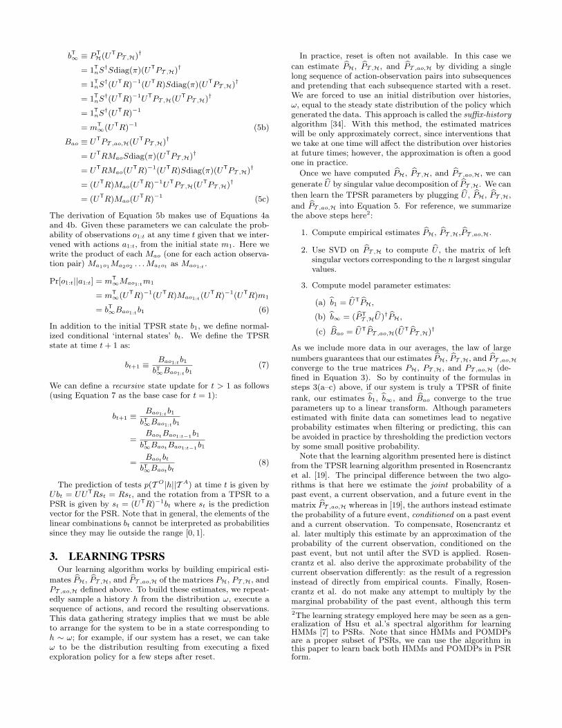
simple 45 × 45 unit square arena with a central obstacleand brightly colored walls (Figure 1(A-B)). We modeled therobot as a sphere of radius 2 units. The robot can movearound the floor of the arena, and rotate to face in any direc-tion. The robot has a simulated 16× 16 pixel color camera,whose focal plane is located one unit in front of the robot’scenter of rotation. The robot’s visual field was 45◦ in bothazimuth and elevation, thus providing the robot with an an-gular resolution of ∼ 2.8◦ per pixel. Images on the sensormatrix at any moment were simulated by a non-linear per-spective transformation of the projected values arising fromthe robot’s position and orientation in the environment at

−8 −4 0 4 8x 10

−3

−4

0

4

x 10−3B.Outer Walls

Inner Walls

A. C.

Simulated Environment Simulated Ebvironment3-d View (to scale)

D.

Learned SubspaceLearned Representation

Mapped to Geometric Space

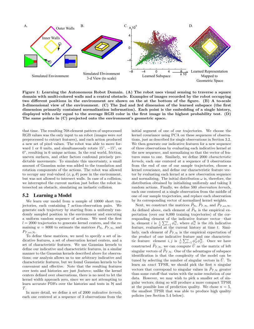
Figure 1: Learning the Autonomous Robot Domain. (A) The robot uses visual sensing to traverse a squaredomain with multi-colored walls and a central obstacle. Examples of images recorded by the robot occupyingtwo different positions in the environment are shown on the at the bottom of the figure. (B) A to-scale3-dimensional view of the environment. (C) The 2nd and 3rd dimension of the learned subspace (the firstdimension primarily contained normalization information). Each point is the embedding of a single history,displayed with color equal to the average RGB color in the first image in the highest probability test. (D)The same points in (C) projected onto the environment’s geometric space.

that time. The resulting 768-element pattern of unprocessedRGB values was the only input to an robot (images were notpreprocessed to extract features), and each action produceda new set of pixel values. The robot was able to move for-ward 1 or 0 units, and simultaneously rotate 15◦, −15◦, or0◦, resulting in 6 unique actions. In the real world, friction,uneven surfaces, and other factors confound precisely pre-dictable movements. To simulate this uncertainty, a smallamount of Gaussian noise was added to the translation androtation components of the actions. The robot was allowedto occupy any real-valued (x, y, θ) pose in the environment,but was not allowed to intersect walls. In case of a collision,we interrupted the current motion just before the robot in-tersected an obstacle, simulating an inelastic collision.

5.2 Learning a ModelWe learn our model from a sample of 10000 short tra-

jectories, each containing 7 action-observation pairs. Wegenerate each trajectory by starting from a uniformly ran-domly sampled position in the environment and executinga uniform random sequence of actions. We used the firstl = 2000 trajectories to generate kernel centers, and the re-maining w = 8000 to estimate the matrices PH, PT ,H, andPT ,ao,H.

To define these matrices, we need to specify a set of in-dicative features, a set of observation kernel centers, and aset of characteristic features. We use Gaussian kernels todefine our indicative and characteristic features, in a similarmanner to the Gaussian kernels described above for observa-tions; our analysis allows us to use arbitrary indicative andcharacteristic features, but we found Gaussian kernels to beconvenient and effective. Note that the resulting featuresover tests and histories are just features; unlike the kernelcenters defined over observations, there is no need to let thekernel width approach zero, since we are not attempting tolearn accurate PDFs over the histories and tests in H andT .

In more detail, we define a set of 2000 indicative kernels,each one centered at a sequence of 3 observations from the

initial segment of one of our trajectories. We choose thekernel covariance using PCA on these sequences of observa-tions, just as described for single observations in Section 3.2.We then generate our indicative features for a new sequenceof three observations by evaluating each indicative kernel atthe new sequence, and normalizing so that the vector of fea-tures sums to one. Similarly, we define 2000 characteristickernels, each one centered at a sequence of 3 observationsfrom the end of one of our sample trajectories, choose akernel covariance, and define our characteristic feature vec-tor by evaluating each kernel at a new observation sequenceand normalizing. The initial distribution ω is, therefore, thedistribution obtained by initializing uniformly and taking 3random actions. Finally, we define 500 observation kernels,each one centered at a single observation from the middle ofone of our sample trajectories, and replace each observationby its corresponding vector of normalized kernel weights.

Next, we construct the matrices bPH, bPT ,H, and bPT ,ao,H.

As defined above, each element of bPH is the empirical ex-pectation (over our 8,000 training trajectories) of the cor-responding element of the indicative feature vector—thatis, element i is 1

w

Pwt=1 φ

Hit , where φHit is the ith indicative

feature, evaluated at the current history at time t. Simi-

larly, each element of bPT ,H is the empirical expectation ofthe product of one indicative feature and one characteris-tic feature: element i, j is 1

w

Pwt=1 φ

TitφHjt. Once we have

constructed bPT ,H, we can compute bU as the matrix of left

singular vectors of bPT ,H. One of the advantages of subspaceidentification is that the complexity of the model can be

tuned by selecting the number of singular vectors in bU . Tolearn an exact TPSR, we should pick the first n singular

vectors that correspond to singular values in bPT ,H greaterthan some cutoff that varies with the noise resolution of ourdata. However, we may wish to pick a smaller set of sin-gular vectors; doing so will produce a more compact TPSRat the possible loss of prediction quality. We chose n = 5,the smallest TPSR that was able to produce high qualitypolicies (see Section 5.4 below).

Estimated Value Function Policies Executed inLearned Subspace

Paths Taken in Geometric Space

−8 −4 0 4 8x 10

−3

−4

0

4

−3

−8 −4 0 4 8x 10

−3

−4

0

4

x 10−3

200

400

600

13.9 18.2

507.8

Num

ber o

f Act

ions

OptimalGreedy Perseus

RandomWalk

0

B.A. D.C.

*

x 10

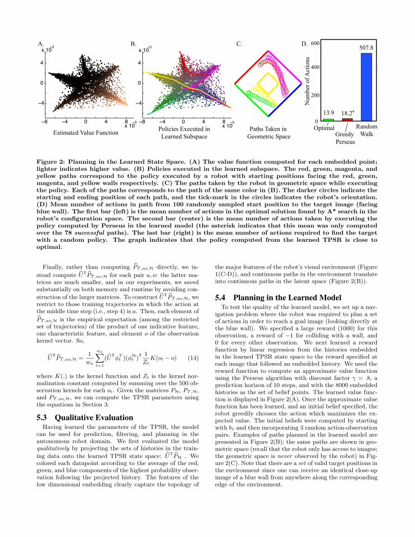
Figure 2: Planning in the Learned State Space. (A) The value function computed for each embedded point;lighter indicates higher value. (B) Policies executed in the learned subspace. The red, green, magenta, andyellow paths correspond to the policy executed by a robot with starting positions facing the red, green,magenta, and yellow walls respectively. (C) The paths taken by the robot in geometric space while executingthe policy. Each of the paths corresponds to the path of the same color in (B). The darker circles indicate thestarting and ending position of each path, and the tick-mark in the circles indicates the robot’s orientation.(D) Mean number of actions in path from 100 randomly sampled start position to the target image (facingblue wall). The first bar (left) is the mean number of actions in the optimal solution found by A* search in therobot’s configuration space. The second bar (center) is the mean number of actions taken by executing thepolicy computed by Perseus in the learned model (the asterisk indicates that this mean was only computedover the 78 successful paths). The last bar (right) is the mean number of actions required to find the targetwith a random policy. The graph indicates that the policy computed from the learned TPSR is close tooptimal.

Finally, rather than computing bPT ,ao,H directly, we in-

stead compute bUT bPT ,ao,H for each pair a, o: the latter ma-trices are much smaller, and in our experiments, we savedsubstantially on both memory and runtime by avoiding con-

struction of the larger matrices. To construct bUT bPT ,ao,H, werestrict to those training trajectories in which the action atthe middle time step (i.e., step 4) is a. Then, each element ofbPT ,ao,H is the empirical expectation (among the restrictedset of trajectories) of the product of one indicative feature,one characteristic feature, and element o of the observationkernel vector. So,

bUT bPT ,ao,H =1

wa

waXt=1

(bUTφTt )(φHt )T 1

ZtK(ot − o) (14)

where K(.) is the kernel function and Zt is the kernel nor-malization constant computed by summing over the 500 ob-servation kernels for each ot. Given the matrices PH, PT ,H,and PT ,ao,H, we can compute the TPSR parameters usingthe equations in Section 3.

5.3 Qualitative EvaluationHaving learned the parameters of the TPSR, the model

can be used for prediction, filtering, and planning in theautonomous robot domain. We first evaluated the modelqualitatively by projecting the sets of histories in the train-

ing data onto the learned TPSR state space: bUT bPH . Wecolored each datapoint according to the average of the red,green, and blue components of the highest probability obser-vation following the projected history. The features of thelow dimensional embedding clearly capture the topology of

the major features of the robot’s visual environment (Figure1(C-D)), and continuous paths in the environment translateinto continuous paths in the latent space (Figure 2(B)).

5.4 Planning in the Learned ModelTo test the quality of the learned model, we set up a nav-

igation problem where the robot was required to plan a setof actions in order to reach a goal image (looking directly atthe blue wall). We specified a large reward (1000) for thisobservation, a reward of −1 for colliding with a wall, and0 for every other observation. We next learned a rewardfunction by linear regression from the histories embeddedin the learned TPSR state space to the reward specified ateach image that followed an embedded history. We used thereward function to compute an approximate value functionusing the Perseus algorithm with discount factor γ = .8, aprediction horizon of 10 steps, and with the 8000 embeddedhistories as the set of belief points. The learned value func-tion is displayed in Figure 2(A). Once the approximate valuefunction has been learned, and an initial belief specified, therobot greedily chooses the action which maximizes the ex-pected value. The initial beliefs were computed by startingwith b1 and then incorporating 3 random action-observationpairs. Examples of paths planned in the learned model arepresented in Figure 2(B); the same paths are shown in geo-metric space (recall that the robot only has access to images;the geometric space is never observed by the robot) in Fig-ure 2(C). Note that there are a set of valid target positions inthe environment since one can receive an identical close-upimage of a blue wall from anywhere along the correspondingedge of the environment.

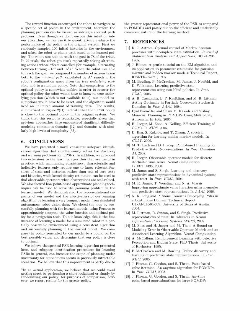
The reward function encouraged the robot to navigate toa specific set of points in the environment, therefore theplanning problem can be viewed as solving a shortest pathproblem. Even though we don’t encode this intuition intoour algorithm, we can use it to quantitatively evaluate theperformance of the policy in the original system. First werandomly sampled 100 initial histories in the environmentand asked the robot to plan a path based on its learned pol-icy. The robot was able to reach the goal in 78 of the trials.In 22 trials, the robot got stuck repeatedly taking alternat-ing actions whose effects cancelled (for example, alternatingbetween turning −15◦ and 15◦).5 When the robot was ableto reach the goal, we compared the number of actions takenboth to the minimal path, calculated by A* search in therobot’s configuration space given the true underlying posi-tion, and to a random policy. Note that comparison to theoptimal policy is somewhat unfair: in order to recover theoptimal policy the robot would have to know its true under-lying position (which is not available to it), our model as-sumptions would have to be exact, and the algorithm wouldneed an unlimited amount of training data. The results,summarized in Figure 2(D), indicate that the TPSR policyis close to the optimal policy in the original system. Wethink that this result is remarkable, especially given thatprevious approaches have encountered significant difficultymodeling continuous domains [12] and domains with simi-larly high levels of complexity [33].

6. CONCLUSIONSWe have presented a novel consistent subspace identifi-

cation algorithm that simultaneously solves the discoveryand learning problems for TPSRs. In addition, we providedtwo extensions to the learning algorithm that are useful inpractice, while maintaining consistency: characteristic andindicative features only require one to know relevant fea-tures of tests and histories, rather than sets of core testsand histories, while kernel density estimation can be used tofind observable operators when observations are real-valued.We also showed how point-based approximate planning tech-niques can be used to solve the planning problem in thelearned model. We demonstrated the representational ca-pacity of our model and the effectiveness of our learningalgorithm by learning a very compact model from simulatedautonomous robot vision data. We closed the loop by suc-cessfully planning with the learned models, using Perseus toapproximately compute the value function and optimal pol-icy for a navigation task. To our knowledge this is the firstinstance of learning a model for a simulated robot in a par-tially observable environment using a consistent algorithmand successfully planning in the learned model. We com-pare the policy generated by our model to a bound on thebest possible value, and determine that our policy is closeto optimal.

We believe the spectral PSR learning algorithm presentedhere, and subspace identification procedures for learningPSRs in general, can increase the scope of planning underuncertainty for autonomous agents in previously intractablescenarios. We believe that this improvement is partly due to

5In an actual application, we believe that we could avoidgetting stuck by performing a short lookahead or simply byrandomizing our policy; for purposes of comparison, how-ever, we report results for the greedy policy.

the greater representational power of the PSR as comparedto POMDPs and partly due to the efficient and statisticallyconsistent nature of the learning method.

7. REFERENCES[1] K. J. Astrom. Optimal control of Markov decision

processes with incomplete state estimation. Journal ofMathematical Analysis and Applications, 10:174–205,1965.

[2] J. Bilmes. A gentle tutorial on the EM algorithm andits application to parameter estimation for gaussianmixture and hidden markov models. Technical Report,ICSI-TR-97-021, 1997.

[3] M. Bowling, P. McCracken, M. James, J. Neufeld, andD. Wilkinson. Learning predictive staterepresentations using non-blind policies. In Proc.ICML, 2006.

[4] A. R. Cassandra, L. P. Kaelbling, and M. R. Littman.Acting Optimally in Partially Observable StochasticDomains. In Proc. AAAI, 1994.

[5] Eyal Even-Dar and Sham M. Kakade and YishayMansour. Planning in POMDPs Using MultiplicityAutomata. In UAI, 2005.

[6] H. Jaeger, M. Zhao, A. Kolling. Efficient Training ofOOMs. In NIPS, 2005.

[7] D. Hsu, S. Kakade, and T. Zhang. A spectralalgorithm for learning hidden markov models. InCOLT, 2009.

[8] M. T. Izadi and D. Precup. Point-based Planning forPredictive State Representations. In Proc. CanadianAI, 2008.

[9] H. Jaeger. Observable operator models for discretestochastic time series. Neural Computation,12:1371–1398, 2000.

[10] M. James and S. Singh. Learning and discoverypredictive state representations in dynamical systemswith reset. In Proc. ICML, 2004.

[11] M. R. James, T. Wessling, and N. A. Vlassis.Improving approximate value iteration using memoriesand predictive state representations. In AAAI, 2006.

[12] N. K. Jong and P. Stone. Towards Employing PSRs ina Continuous Domain. Technical ReportUT-AI-TR-04-309, University of Texas at Austin,2004.

[13] M. Littman, R. Sutton, and S. Singh. Predictiverepresentations of state. In Advances in NeuralInformation Processing Systems (NIPS), 2002.

[14] M. Zhao and H. Jaeger and M. Thon. A Bound onModeling Error in Observable Operator Models and anAssociated Learning Algorithm. Neural Computation.

[15] A. McCallum. Reinforcement Learning with SelectivePerception and Hidden State. PhD Thesis, Universityof Rochester, 1995.

[16] P. McCracken and M. Bowling. Online discovery andlearning of predictive state representations. In Proc.NIPS, 2005.

[17] J. Pineau, G. Gordon, and S. Thrun. Point-basedvalue iteration: An anytime algorithm for POMDPs.In Proc. IJCAI, 2003.

[18] J. Pineau, G. Gordon, and S. Thrun. Anytimepoint-based approximations for large POMDPs.

Journal of Artificial Intelligence Research (JAIR),27:335–380, 2006.

[19] M. Rosencrantz, G. J. Gordon, and S. Thrun.Learning low dimensional predictive representations.In Proc. ICML, 2004.

[20] S. Ross and J. Pineau. Model-Based BayesianReinforcement Learning in Large Structured Domains.In Proc. UAI, 2008.

[21] G. Shani, R. I. Brafman, and S. E. Shimony.Model-based online learning of POMDPs. In Proc.ECML, 2005.

[22] S. M. Siddiqi, B. Boots, and G. J. Gordon.Reduced-Rank Hidden Markov Models.http://arxiv.org/abs/0910.0902, 2009.

[23] B. W. Silverman. Density Estimation for Statisticsand Data Analysis. Chapman & Hall, 1986.

[24] S. Singh, M. James, and M. Rudary. Predictive staterepresentations: A new theory for modeling dynamicalsystems. In Proc. UAI, 2004.

[25] S. Singh, M. L. Littman, N. K. Jong, D. Pardoe, andP. Stone. Learning predictive state representations. InProc. ICML, 2003.

[26] S. Soatto and A. Chiuso. Dynamic data factorization.Technical report, UCLA, 2001.

[27] E. J. Sondik. The Optimal Control of PartiallyObservable Markov Processes. PhD. Thesis, StanfordUniversity, 1971.

[28] M. T. J. Spaan and N. Vlassis. Perseus: Randomizedpoint-based value iteration for POMDPs. Journal ofArtificial Intelligence Research, 24:195–220, 2005.

[29] P. Van Overschee and B. De Moor. SubspaceIdentification for Linear Systems: Theory,Implementation, Applications. Kluwer, 1996.

[30] E. Wiewiora. Learning predictive representations froma history. In Proc. ICML, 2005.

[31] D. Wingate. Exponential Family PredictiveRepresentations of State. PhD Thesis, University ofMichigan, 2008.

[32] D. Wingate and S. Singh. On discovery and learningof models with predictive representations of state foragents with continuous actions and observations. InProc. AAMAS, 2007.

[33] D. Wingate and S. Singh. Efficiently learninglinear-linear exponential family predictiverepresentations of state. In Proc. ICML, 2008.

[34] B. Wolfe, M. James, and S. Singh. Learning predictivestate representations in dynamical systems withoutreset. In Proc. ICML, 2005.