Embed Size (px)
Citation preview
CHAPTER 14
Closed population capture-recapture models
Paul Lukacs, University of Montana
A fair argument could be made that the marking of individuals in a wild population was originally
motivated by the desire to estimate a fundamental parameter: abundance (i.e., population size). By
comparing the relative proportions of marked and unmarked animals in successive samples, various
estimators of animal abundance could be derived. In this chapter, we consider the theory and mechanics
of estimation of abundance from closed population capture-recapture data, using program MARK.∗
Here, the population of interest is assumed to be closed geographically – no movement on or off the
study area – and demographically – no births or deaths.
14.1. The basic idea
How many individuals are there in the sampled population? Well, if the population is (or assumed
to be) closed, then the number of individuals in the population being sampled is a constant over time.
Meaning, the population size does not change at each sampling event. With a little thought, you quickly
realize that the canonical estimate of population size is a function of (i) how many unique individuals
are encountered over all sampling events, and (ii) what the probability is of encountering an individual
at least once. For a single sampling event, we can express this more formally as
N �n
p,
where the numerator (n) is the number of unique individuals encountered, and the denominator (p) is
the probability that any individual will be encountered.
This expression makes good intuitive sense. For example, suppose that you capture 50 individuals
(n � 50), and the encounter probability is p � 0.5, then clearly, since there is a 50:50 chance that you
will miss an individual instead of encountering it, then
N �n
p�
50
0.5� 100.
∗ Prior to MARK, program CAPTURE was a widely used application for closed population abundance estimation. All of thelikelihood-based models from CAPTURE can be built in MARK, plus numerous models that have been developed since then.Further, there are some important differences between MARK and CAPTURE: (i) for likelihood-based models, CAPTUREreturns the estimate from the integer, and not the floating point value that maximizes the likelihood; (ii) all of the heterogeneitymodels in CAPTURE (except Mbh) are not likelihood based, so will give quite different estimates than those from MARK.
© Cooch & White (2018) 04.23.2018
14.1.1. The Lincoln-Petersen estimator – a quick review 14 - 2
14.1.1. The Lincoln-Petersen estimator – a quick review
The most general approach to estimating abundance, and p, in closed populations is based on what is
known as the Lincoln-Petersen estimator (hereafter, the ‘LP’ estimator). The LP estimator is appropriate
when there are just two sampling occasions, and the population is closed between the two occasions.
Imagine you go out on the first occasion, capture a sample of individuals, mark and release them
back into the population. On the second occasion, you re-sample from (what you hope is) the same
population. In this second sample, there will be two types of individuals: those that are unmarked (not
previously captured) and those with marks (individuals captured and marked on the first occasion).
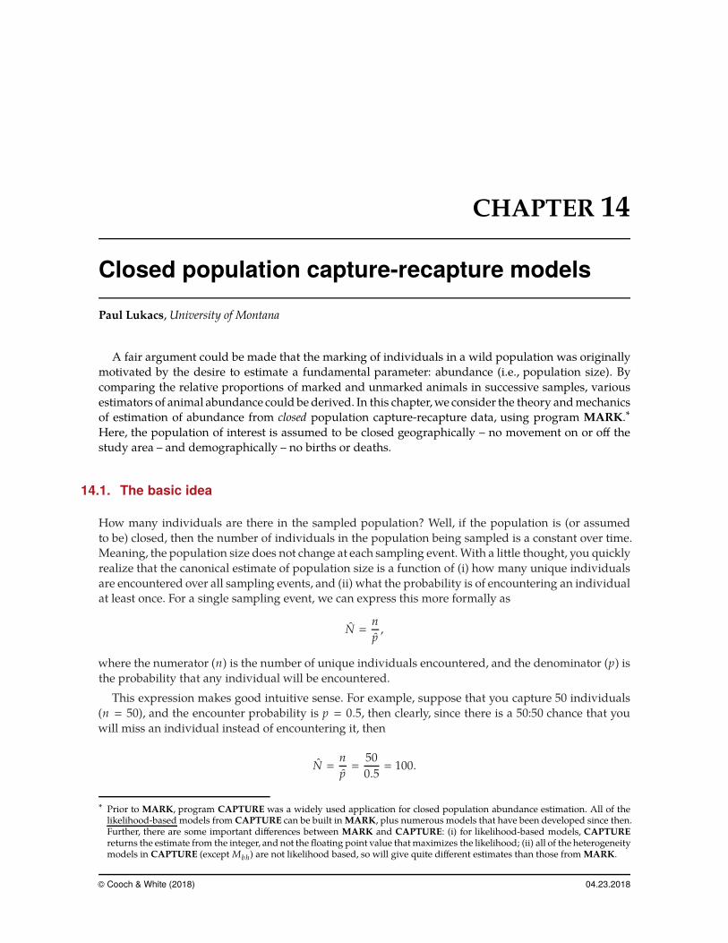
The basic sampling structure is shown in Fig. (14.1).
marked ( )n1
previouslymarked ( )m2
firstsample marked ( )n1
secondsample
totalpopulation
samplingoccasion 1
samplingoccasion 2
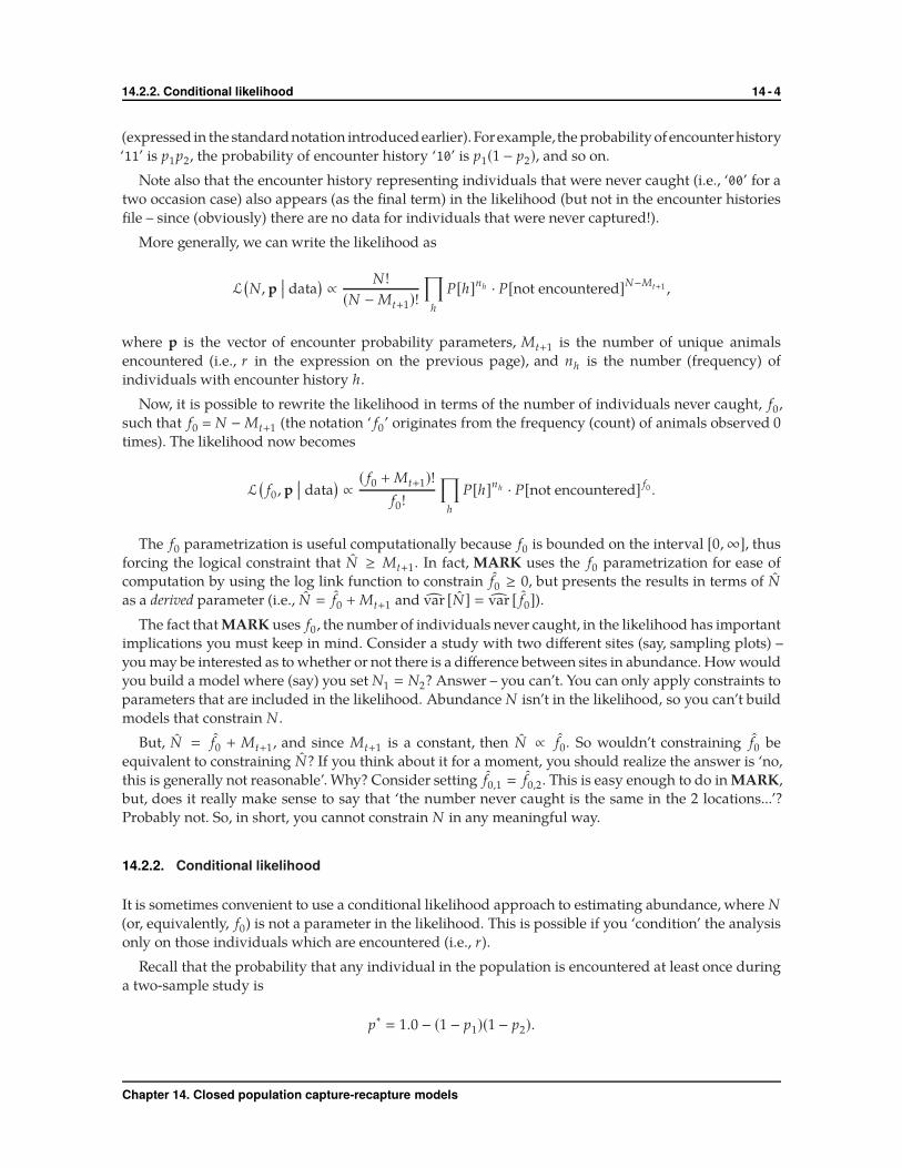
Figure 14.1: Schematic representation of the LP sampling scheme. The entire left-most vertical bar (the sum oflight- and dark-grey areas) represents the total population, N. The light-grey represents the proportion of thetotal population that is sampled on the first sampling occasion. The number encountered, and marked, duringthis first sample, is n1. The middle bar is the same population at the time of the second sample, with the same totalabundance,N,which we assume is constant between sampling occasions. During the second sample, indicated asthe proportion of the total population bounded by the dashed-line box, some of the n2 total sampled individualsare newly encountered – dark-grey – while some (m2, the light-grey portion) were previously encountered.Adapted from Powell & Gale 2015.
We develop the LP estimator by noting that the proportion of marked animals in the population
after the first sample is simply n1/N , where N is the size of the population (and which, of course, is
what we’re trying to estimate). Note that the numerator of this expression (n1) is known, whereas the
denominator (N) is not. In the second sample (Fig. 14.1), the ratio of the previously marked to the total
number of individuals sampled is, simply, m2/n2.
Now, the key step, based on the following assumption – we assume that all individuals (marked or
not) are equally catchable (meaning, we assume random mixing of marked and unmarked after the first
sample). Under this assumption, then this proportion of previously marked individuals in the second
sample should be equivalent to the proportion of newly marked individuals in the first sample:
m2
n2
�
n1
N.
Chapter 14. Closed population capture-recapture models
14.2. Likelihood 14 - 3
Next, a little algebraic rearrangement of this equation, and we come up with the familiar LP estimator
for abundance, as
N �
n1n2
m2
.
We might also use the canonical form noted earlier, where abundance is estimated as the count
statistic divided by the encounter probability:
N �n
p.
If n1 is the number of animals caught and marked at the first sampling occasion, and if m2 is the
number of the animals caught in both occasions, then assuming that (i) all n1 individuals are alive and
in the sample at occasion 2, and (ii) that marked and unmarked individuals have the same probability
of detection, then the probability of encountering any of those n1 marked individuals is
p �
m2
n2
.
Thus, the ratio of the count statistic to the detection probability is the Lincoln-Petersen estimator:
N �
n1
p�
n1n2
m2
.
14.2. Likelihood
While the ‘algebraic’ (LP) estimator for N developed in the preceding section is simple, reasonably
intuitive and undoubtedly quite familiar, here we consider a more formal approach, based upon
maximum likelihood estimation.
14.2.1. Full likelihood approach
We start by re-visiting the simple two sample study we used to motivate the LP estimator introduced
in the previous section. For such a study, there are only 4 possible encounter histories: ‘11’, ‘10’, ‘01’,
and ‘00’. The number of individuals with encounter history ‘00’ is not known directly, but must be
estimated. So, the estimation of abundance proceeds by using the number of individuals observed who
were encountered at least once.
We can express the probability distribution for n1, n2 , and m2, given the r (total) observed frequencies
of the 3 observable encounter histories ( ‘11’, ‘10’ and ‘01’), as
P(n1 , n2 ,m2
�� N, p1, p2
)�
N!
m2!(n1 − m1
)!(n2 − m2
)!(N − r)!
×(p1p2
)m2[p1
(1 − p2
) ] (n1−m2)[ (
1 − p1
)p2
] (n2−m2)[ (
1 − p1
) (1 − p2
) ] (N−r).
Two important things to note in this expression. First, N appears in the multinomial coefficient of the
likelihood function. Second, the probability expression is written including a term for each encounter
history, and with the exponent representing the number of individuals with a given encounter history
Chapter 14. Closed population capture-recapture models
14.2.2. Conditional likelihood 14 - 4
(expressed in the standardnotation introducedearlier). Forexample, the probability of encounterhistory
‘11’ is p1p2, the probability of encounter history ‘10’ is p1(1 − p2), and so on.
Note also that the encounter history representing individuals that were never caught (i.e., ‘00’ for a
two occasion case) also appears (as the final term) in the likelihood (but not in the encounter histories
file – since (obviously) there are no data for individuals that were never captured!).
More generally, we can write the likelihood as
L(N, p
�� data)∝
N!
(N − Mt+1)!
∏
h
P[h]nh · P[not encountered]N−Mt+1 ,
where p is the vector of encounter probability parameters, Mt+1 is the number of unique animals
encountered (i.e., r in the expression on the previous page), and nh is the number (frequency) of
individuals with encounter history h.
Now, it is possible to rewrite the likelihood in terms of the number of individuals never caught, f0,
such that f0 = N − Mt+1 (the notation ‘ f0’ originates from the frequency (count) of animals observed 0
times). The likelihood now becomes
L(
f0 , p�� data
)∝
( f0 + Mt+1)!
f0!
∏
h
P[h]nh · P[not encountered] f0 .
The f0 parametrization is useful computationally because f0 is bounded on the interval [0,∞], thus
forcing the logical constraint that N ≥ Mt+1. In fact, MARK uses the f0 parametrization for ease of
computation by using the log link function to constrain f0 ≥ 0, but presents the results in terms of N
as a derived parameter (i.e., N � f0 + Mt+1 and var [N] � var [ f0]).
The fact that MARK uses f0, the number of individuals never caught, in the likelihood has important
implications you must keep in mind. Consider a study with two different sites (say, sampling plots) –
you may be interested as to whether or not there is a difference between sites in abundance. How would
you build a model where (say) you set N1 � N2? Answer – you can’t. You can only apply constraints to
parameters that are included in the likelihood. Abundance N isn’t in the likelihood, so you can’t build
models that constrain N .
But, N � f0 + Mt+1, and since Mt+1 is a constant, then N ∝ f0. So wouldn’t constraining f0 be
equivalent to constraining N? If you think about it for a moment, you should realize the answer is ‘no,
this is generally not reasonable’. Why? Consider setting f0,1 � f0,2. This is easy enough to do in MARK,
but, does it really make sense to say that ‘the number never caught is the same in the 2 locations...’?
Probably not. So, in short, you cannot constrain N in any meaningful way.
14.2.2. Conditional likelihood
It is sometimes convenient to use a conditional likelihood approach to estimating abundance, where N
(or, equivalently, f0) is not a parameter in the likelihood. This is possible if you ‘condition’ the analysis
only on those individuals which are encountered (i.e., r).
Recall that the probability that any individual in the population is encountered at least once during
a two-sample study is
p∗� 1.0 − (1 − p1)(1 − p2).
Chapter 14. Closed population capture-recapture models
14.2.2. Conditional likelihood 14 - 5
Thus, we can re-write the conditional probability expression for the capture histories as
P({xi j}
�� r, p1 , p2
)�
r!
x11!x10!x01!×
(p1p2
p∗
)x11(
p1
(1 − p2
)
p∗
)x10( (
1 − p1
)p2
p∗
)x01
.
The ML estimates for this model are again fairly easy to derive (see Williams, Nichols & Conroy 2002
for the details).
The primary advantage of using this conditional likelihood approach is that individual covariates can
be used to model the encounter process. Individual covariates cannot be used with the full likelihood
approach introduced in the preceding section, because the term (1 − p1)(1 − p2) . . . (1 − pt) is included
in the likelihood, and no covariate value is available for animals that were never captured.
In contrast, the unconditional likelihood approach conditions this multinomial term out of the
likelihood, and so an individual covariate can be measured for each of the animals included in the
likelihood. When individual covariates are used, a Horvitz-Thompson estimator is used to estimate N :
N �
Mt+1∑
i�1
1
1 −[1 − p1(xi)
] [1 − p2(xi)
]...
[1 − pt(xi)
] .
An example is perhaps the best way to illustrate the difference between the full and conditional
likelihood approaches. Consider the 4 possible encounter histories for 2 sampling occasions:
encounter history probability
11 p1p2
10 p1
(1 − p2
)
01(1 − p1
)p2
00(1 − p1
) (1 − p2
)
For each of the encounter histories except the last, the number of animals with the specific encounter
history is known. For the last encounter history, the number of animals is f0 � (N − Mt+1), i.e., the
population size (N) minus the number of animals known to have been in the population (Mt+1).
The approach (first described by Huggins 1989, 1991) was to condition this last encounter history out
of the likelihood by dividing the quantity ‘1 minus this last history’ into each of the others. The result
is a new multinomial distribution that still sums to one. The derived parameter N is then estimated as
N �
Mt+1[1 −
(1 − p
) (1 − p
) (1 − p
) ] ,
for data with no individual covariates. A more complex estimator is required for models that include
individual covariates to model the p parameters.
Here’s a simple example of how this works, given 2 occasions. Let p1 � 0.4, p2 � 0.3. At the top of
the next page, we tabulate both the unconditional probability of a given encounter history (i.e., where N
is in the likelihood), and the conditional probability of the encounter history, where the individuals not
seen are not included (i.e., are ‘conditioned out’). Note that if p1 � 0.4 and p2 � 0.3, then the probability
of not being captured at all is (1− p1)(1− p2) � 0.42, such that the probability of being captured at least
once is p∗� (1 − 0.42) � 0.58.
Chapter 14. Closed population capture-recapture models
14.2.2. Conditional likelihood 14 - 6
history unconditional Pr(history) Pr(history | captured)
11 p1p2 (0.4 × 0.3) � 0.12(p1p2
)/p∗ 0.12/0.58 � 0.207
10 p1
(1 − p2
)0.4 (1 − 0.3) � 0.28
[p1
(1 − p2
) ]/p∗ 0.28/0.58 � 0.483
01 (1 − p1)p2 (1 − 0.4) 0.3 � 0.18[ (
1 − p1
)p2
]/p∗ 0.18/0.58 � 0.310
00(1 − p1
) (1 − p2
)(1 − 0.4)(1 − 0.3) � 0.42 (not included because not captured)
In either case, the probabilities for all 4 histories sum to 1.0 (i.e., (0.12+ 0.28+ 0.18+ 0.42) � 1.0, and
(0.207 + 0.48 + 0.310) � 1.0). Each forms a multinomial likelihood that can be solved for p1 and p2, by
maximizing the likelihood expression.
As noted earlier, the derived parameter N is then estimated as
N �
Mt+1[1 −
(1 − p
) (1 − p
) (1 − p
) ] ,
for data with no individual covariates.
Regardless of whether or not you include individuals not encountered in the likelihood, the key to
understanding the fitting of closed capture models is in realizing that the event histories are governed
entirely by the encounter probability.
In fact, the process of estimating abundance for closed models is in effect the process of estimating
detection probabilities – the probability that an animal will be caught for the first time (if at all), and the
probability that if caught at least once, that it will be caught again. The different closed population
models differ conceptually on how variation in the encounter probability (e.g., over time, among
individuals) is handled. The mechanics of fitting these models in MARK is the subject of the rest
of this chapter.
begin sidebar
What does ‘closure’ really mean?
The ‘closed captures’ data types all assume the population of interest is closed during the sampling
period (White et al. 1982). Meaning, the models assume that no births or deaths occur and no
immigration or emigration occurs. Typically, we refer to a closed population as one that is free of
unknown changes in abundance, as we can usually account for known changes.
A few methods have been developed to test for closure violations. Program CloseTest (Stanley &
Burnham 1999) can test the assumption of closure in some cases, although it is no longer in widespread
use. The Pradel model with ‘survival and recruitment’ parameterization has also been used to
explore closure violations (Boulanger et al. 2002; see chapter 13 for details of the Pradel model),
and offers some flexibility. By analyzing closed population capture-recapture data with the Pradel
‘survival and recruitment’ parameterization, one could test for closure and violations of closure.
For example, a model with ϕ fixed to 1 (no losses), and f fixed to 0 (no entries) would represent a
model with ‘full closure’, and could be compared to a model where both ϕ and f are unconstrained.
To test violations of closure due to emigration, you could construct a model with ϕ fixed to 1, with f
unconstrained. Alternatively, to test for violation of closure due to immigration, you could construct
a model with f fixed to 0, with ϕ unconstrained.
Heterogeneity in capture probability can cloud our ability to detect closure violations. In situations
where the population is truly closed, heterogeneity in capture probability can cause both the tests of
immigration and emigration to reject the null hypothesis of closure.
end sidebar
Chapter 14. Closed population capture-recapture models
14.3. Model types 14 - 7
14.3. Model types
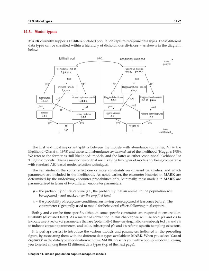
MARK currently supports 12 different closed population capture-recapture data types. These different
data types can be classified within a hierarchy of dichotomous divisions – as shown in the diagram,
below:
full likelihood conditional likelihood
full mixtures + mis-ID
f0, , , ,p c a p
mixtures + mis-ID
f p0, , ,a p
p cº
closed captures + mis-ID
f ,0, ,p c a
full mixtures
f ,0, ,p c p
mixtures
f p0, ,pclosed captures
f0, ,p c
Mo
f p0,
p=1c=1
pºc
a=1
p=1a=1
p cºp=1
Huggins full mixtures+ mis-ID p c, , ,a p
Huggins mixtures + mis-ID
p, ,a p
p cº
Huggins closed captures+ mis-ID p c, ,a
Huggins full mixturesp c, ,p
Huggins mixturesp,p
Huggins closed captures
p c,
Huggins Mo
p
p=1c=1
p cº
a=1
p=1a=1
p cºp=1
p M| t+1
moregeneral
moreconstrained
The first and most important split is between the models with abundance (or, rather, f0) in the
likelihood (Otis et al. 1978) and those with abundance conditioned out of the likelihood (Huggins 1989).
We refer to the former as ‘full likelihood’ models, and the latter as either ‘conditional likelihood’ or
‘Huggins’ models. This is a major division that results in the two types of models not being comparable
with standard AIC-based model selection techniques.
The remainder of the splits reflect one or more constraints on different parameters, and which
parameters are included in the likelihoods. As noted earlier, the encounter histories in MARK are
determined by the underlying encounter probabilities only. Minimally, most models in MARK are
parameterized in terms of two different encounter parameters:
p – the probability of first capture (i.e., the probability that an animal in the population will
be captured – and marked - for the very first time)
c – the probability of recapture (conditional on having been captured at least once before). The
c parameter is generally used to model for behavioral effects following inial capture.
Both p and c can be time specific, although some specific constraints are required to ensure iden-
tifiability (discussed later). As a matter of convention in this chapter, we will use bold p’s and c’s to
indicate a set (vector) of parameters that are (potentially) time varying, italic, un-subscripted p’s and c’s
to indicate constant parameters, and italic, subscripted p’s and c’s refer to specific sampling occasions.
It is perhaps easiest to introduce the various models and parameters indicated in the preceding
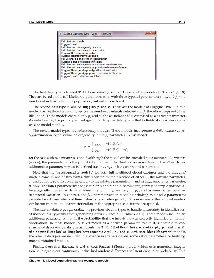
figure, by associating them with the different data types available in MARK. When you select ’closed
captures’ in the data type specification window, MARK presents you with a popup window allowing
you to select among these 12 different data types (top of the next page).
Chapter 14. Closed population capture-recapture models
14.3. Model types 14 - 8
The first data type is labeled ‘Full Likelihood p and c’. These are the models of Otis et al. (1978).
They are based on the full likelihood parametrization with three types of parameters; pi , ci , and f0 (the
number of individuals in the population, but not encountered).
The second data type is labeled ‘Huggins p and c’. These are the models of Huggins (1989). In this
model, the likelihood is conditioned on the number of animals detected and f0 therefore drops out of the
likelihood. These models contain only pi and ci ; the abundance N is estimated as a derived parameter.
As noted earlier, the primary advantage of the Huggins data type is that individual covariates can be
used to model p and c.
The next 4 model types are heterogeneity models. These models incorporate a finite mixture as an
approximation to individual heterogeneity in the pi parameter. In this model,
pi �
{pi ,A with Pr(π)
pi ,B with Pr(1 − π),
for the case with two mixtures A and B, although the model can be extended to >2 mixtures. As written
(above), the parameter π is the probability that the individual occurs in mixture A. For >2 mixtures,
additional π parameters must be defined (i.e., πA , πB ,...), but constrained to sum to 1.
Note that the ‘heterogeneity models’ for both full likelihood closed captures and the Huggins’
models come in one of two forms, differentiated by the presence of either (i) the mixture parameter,
π, and both the pi and ci parameters, or (ii) the mixture parameter,π, and a single encounter parameter,
p, only. The latter parameterizations (with only the π and p parameters) represent simple individual
heterogeneity models, with parameters π, pi ,A � pA, and pi ,B � pB , and assume no temporal or
behavioral variation. In contrast, the full parametrization models (including π, p and c parameters)
provide for all three effects of time, behavior, and heterogeneity. Of course, any of the reduced models
can be run from the full parameterizations if the appropriate constraints are applied.
The next six data types generalize the previous six data types to handle uncertainty in identification
of individuals, typically from genotyping error (Lukacs & Burnham 2005). These models include an
additional parameter, α, that is the probability that the individual was correctly identified on its first
observation. In these models, N is estimated as a derived parameter. While it is possible to con-
struct models for every data type using only the ‘Full Likelihood heterogeneity pi, p, and c with
mis-identification’ or ‘Huggins heterogeneity pi, p, and c with mis-identification’ models,
the other data types are included to allow the user a less cumbersome set of parameters for building
more constrained models.
Finally, there is a ‘Huggins p and c with Random Effects’ model, which uses numerical integra-
tion to integrate out continuous, individual random differences in latent encounter probability. This
Chapter 14. Closed population capture-recapture models
14.3.1. Constraining the final p 14 - 9
approach is conceptually somewhat ‘outside’ the simple ‘full likelihood’ versus ‘conditional likelihood’
models split introduced earlier.
The heterogeneity, misidentification and random effects models will be treated in more detail later
in this chapter.
14.3.1. Constraining the final p
A subtlety of the closed population models is that the last p parameter is not identifiable unless a
constraint is imposed. When no constraint is imposed on the last pi , the likelihood is maximized with
the last p � 1, giving the estimate N � Mt+1. Why?
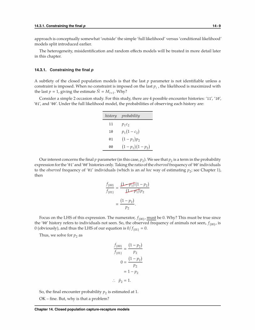
Consider a simple 2 occasion study. For this study, there are 4 possible encounter histories: ‘11’, ‘10’,
‘01’, and ‘00’. Under the full likelihood model, the probabilities of observing each history are:
history probability
11 p1c2
10 p1
(1 − c2
)
01(1 − p1
)p2
00(1 − p1
) (1 − p2
)
Our interest concerns the final p parameter (in this case, p2). We see that p2 is a term in the probability
expression for the ‘01’ and ‘00’ histories only. Taking the ratio of the observed frequency of ‘00‘ individuals
to the observed frequency of ‘01’ individuals (which is an ad hoc way of estimating p2; see Chapter 1),
then
f{00}
f{01}
�✘✘✘✘(1 − p1
) (1 − p2
)
✘✘✘✘(1 − p1
)p2
�
(1 − p2
)
p2
.
Focus on the LHS of this expression. The numerator, f{00}, must be 0. Why? This must be true since
the ‘00’ history refers to individuals not seen. So, the observed frequency of animals not seen, f{00}, is
0 (obviously), and thus the LHS of our equation is 0/ f{01} � 0.
Thus, we solve for p2 as
f{00}
f{01}
�
(1 − p2
)
p2
0 �
(1 − p2
)
p2
� 1 − p2
∴ p2 � 1.
So, the final encounter probability p2 is estimated at 1.
OK – fine. But, why is that a problem?
Chapter 14. Closed population capture-recapture models
14.4. Encounter histories format 14 - 10
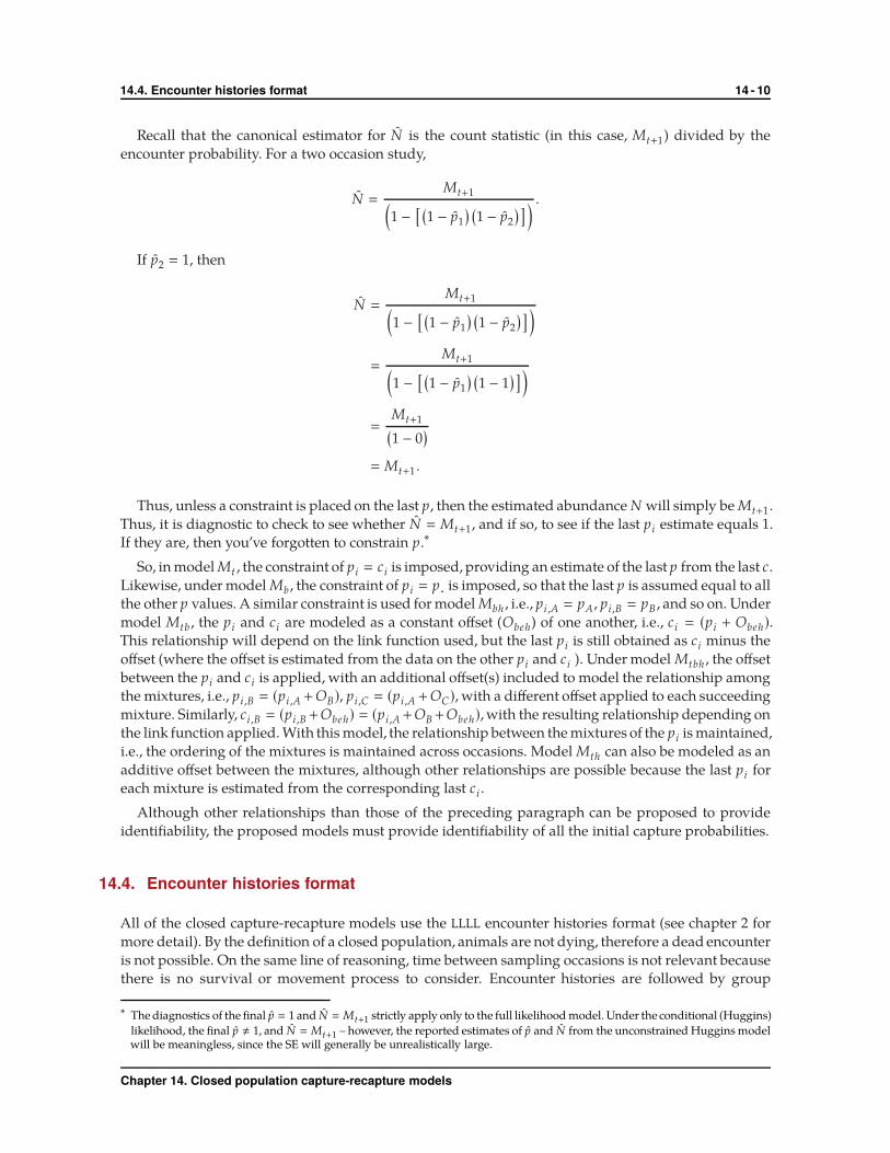
Recall that the canonical estimator for N is the count statistic (in this case, Mt+1) divided by the
encounter probability. For a two occasion study,
N �
Mt+1(1 −
[ (1 − p1
) (1 − p2
) ] ) .
If p2 � 1, then
N �
Mt+1(1 −
[ (1 − p1
) (1 − p2
) ] )
�
Mt+1(1 −
[ (1 − p1
) (1 − 1
) ] )
�
Mt+1(1 − 0
)
� Mt+1 .
Thus, unless a constraint is placed on the last p, then the estimated abundance N will simply be Mt+1.
Thus, it is diagnostic to check to see whether N � Mt+1, and if so, to see if the last pi estimate equals 1.
If they are, then you’ve forgotten to constrain p.∗
So, in model Mt , the constraint of pi � ci is imposed, providing an estimate of the last p from the last c.
Likewise, under model Mb , the constraint of pi � p· is imposed, so that the last p is assumed equal to all
the other p values. A similar constraint is used for model Mbh , i.e., pi ,A � pA, pi ,B � pB , and so on. Under
model Mtb , the pi and ci are modeled as a constant offset (Obeh) of one another, i.e., ci � (pi + Obeh).
This relationship will depend on the link function used, but the last pi is still obtained as ci minus the
offset (where the offset is estimated from the data on the other pi and ci ). Under model Mtbh , the offset
between the pi and ci is applied, with an additional offset(s) included to model the relationship among
the mixtures, i.e., pi ,B � (pi ,A +OB), pi ,C � (pi ,A +OC), with a different offset applied to each succeeding
mixture. Similarly, ci ,B � (pi ,B +Obeh) � (pi ,A +OB+Obeh), with the resulting relationship depending on
the link function applied. With this model, the relationship between the mixtures of the pi is maintained,
i.e., the ordering of the mixtures is maintained across occasions. Model Mth can also be modeled as an
additive offset between the mixtures, although other relationships are possible because the last pi for
each mixture is estimated from the corresponding last ci .
Although other relationships than those of the preceding paragraph can be proposed to provide
identifiability, the proposed models must provide identifiability of all the initial capture probabilities.
14.4. Encounter histories format
All of the closed capture-recapture models use the LLLL encounter histories format (see chapter 2 for
more detail). By the definition of a closed population, animals are not dying, therefore a dead encounter
is not possible. On the same line of reasoning, time between sampling occasions is not relevant because
there is no survival or movement process to consider. Encounter histories are followed by group
∗ The diagnostics of the final p � 1 and N � Mt+1 strictly apply only to the full likelihood model. Under the conditional (Huggins)
likelihood, the final p , 1, and N � Mt+1 – however, the reported estimates of p and N from the unconstrained Huggins modelwill be meaningless, since the SE will generally be unrealistically large.
Chapter 14. Closed population capture-recapture models

14.5. Building models 14 - 11
frequencies. For the Huggins models, group frequencies can be followed with individual covariates.
All encounter histories end with the standard semicolon.
/* Closed capture-recapture data for a Huggins model.
tag #, encounter history, males, females, length */
/* 001 */ 1001 1 0 22.3;
/* 002 */ 0111 1 0 18.9;
/* 003 */ 0100 0 1 20.6;
If you wish to analyze a data set that contains covariates in the input with both full and conditional
likelihoods, you must initially import that data set by selecting a ‘Huggins’ data type. The ‘Closed
Captures’ data type will not allow individual covariates to be specified. In this case, it is likely best to
create two separate MARK files for the analysis because the AICc values are not comparable between
the ‘Closed Captures’ and ‘Huggins’ data types.
14.5. Building models
Now it is time to move on to the actual mechanics of closed population abundance estimation in MARK.
We will analyze some simulated data contained in (simple_closed1.inp). In this simulated data set
(which consists of 6 encounter occasions), true N � 350. The total number of individuals encountered
was Mt+1 � 339 (so, 11 individuals were never seen). Open MARK and create a new database using
the ‘File | New’ option. Select the ‘Closed Captures’ radio-button. When you click on the ‘Closed
Captures’ radio-button, a window will open that allows you to select a model type, shown earlier in
this chapter. To start, select ‘Full Likelihood p and c’.
Enter a title, select the input file, and set the number of encounter occasions to 6.
To start, we’ll construct some of the ‘standard’ closed capture models, as originally described in Otis
et al. (1978). Model notation for the closed capture-recapture models in the literature often still follows
that of Otis et al. (1978). Now that more complex models can be built, it seems appropriate to use a
notation that is similar to the notation used for other models in MARK. Thus, our notation in this
chapter will be based on a description of the parameters in the models.
Below,we present a table contrasting model notation based on Otis et al. (1978) and expanded notation
based on a description of the parameters. Combinations of the models described are possible.
Otis notation Expanded notation Description
M0 { f0 , p(·) � c(·)} Constant p
Mt { f0 , p(t) � c(t)} Time varying p
Mb { f0 , p(·), c(·)} Behavioral response
Mh or Mh2 { f0 , pa(·) � ca(·), pb(·) � cb(·), π} Heterogeneous p
If you look closely at the ‘expanded notation’, you’ll see that models are differentiated based on
Chapter 14. Closed population capture-recapture models

14.5. Building models 14 - 12
relationships between the p and c parameters. This is important – the closed capture-recapture models
are one of the model types in MARK where different types of parameters are modeled as functions of
each other. In this case p and c are commonly modeled as functions of one another. This makes intuitive
sense because both p and c relate to catching animals.
With that said, let’s begin building a few models to learn the mechanics of using MARK to estimate
abundance. We’ll start with models { f0 , p(·) � c(·)}, { f0 , p(t) � c(t)}, and { f0 , p(·), c(·)} (i.e., models
M0 ,Mt and Mb).
Let’s first examine the default PIM chart for the ‘Full Likelihood p and c’ models:
MARK defaults to a time-varying parameter structure where there is a different p and c for each
occasion. Recall from section 14.3.1 that abundance is not estimable with this model structure because
no constraint is imposed to estimate p10. If this default, fully time-dependent model is fit to the data,
N � Mt+1 and p10 � 1.0 regardless of the data. Therefore, in every model we build we must put some
constraint on pi for the last encounter occasion so that this parameter is estimated.
If we open the PIM windows, we’ll notice that the p’s and c’s have only a single row of text boxes.
For example, for p:
Chapter 14. Closed population capture-recapture models

14.5. Building models 14 - 13
In the closed capture models, every individual is assumed to be in the population and at risk of
capture on every occasion. Therefore, there is no need for cohorts (expressed as multiple rows in the
PIM window) as there is for many of the open-population models.
We’ll start with { f0 , p(·) � c(·)} – for this model, there is no temporal variation in either p or c, and
the two parameters are set equal to each other. This model is easily constructed using the PIM chart:
Go ahead and run this model, and add the results to the browser. Couple of important things to
note. First, it is common for AICc values to be negative for the full likelihood closed captures models.
Negative AICc values are legitimate and interpreted in the same way as positive AICc values. The
negative AIC arises due to the portion of the multinomial coefficient that is computed. Recall that for
the full likelihood for the 2-sample situation, the multinomial coefficient was written as
N!
m2!(n1 − m1
)!(n2 − m2
)!(N − r)!
≡
(f0 + Mt+1
)!
m2!(n1 − m1
)!(n2 − m2
)! f0!,
which, after dropping terms that did not include N (or f0), simplifies to
(f0 + Mt+1
)!
✚✚m2!✘✘✘✘✘(
n1 − m1
)!✘✘✘✘✘(
n2 − m2
)! f0!
∝( f0 + Mt+1)!
f0!,
which is frequently negative (which results in a negative AICc). In contrast, AICc values from the
conditional likelihood models are typically positive. Regardless, the model with the ‘most negative’
AICc , i.e., the one furthest from zero, is the most parsimonious model.
Also, note that MARK defaults to a sin link, just as it does with all other data types when an identity
design matrix is specified. In the case of the closed models, the sin link is used for the p’s and c’s, but
a log link is used for f0. The log link is used because f0 must be allowed to be in the range of [0 → ∞].
Therefore, no matter what link function you select, a log link will be used on f0. If you choose the
‘Parm-Specific’ option to set different link functions for each parameter, be sure you choose a link that
does not constrain f0 to the [0, 1] interval. Choose either a log or identity link (log is preferable).
Chapter 14. Closed population capture-recapture models
14.5. Building models 14 - 14
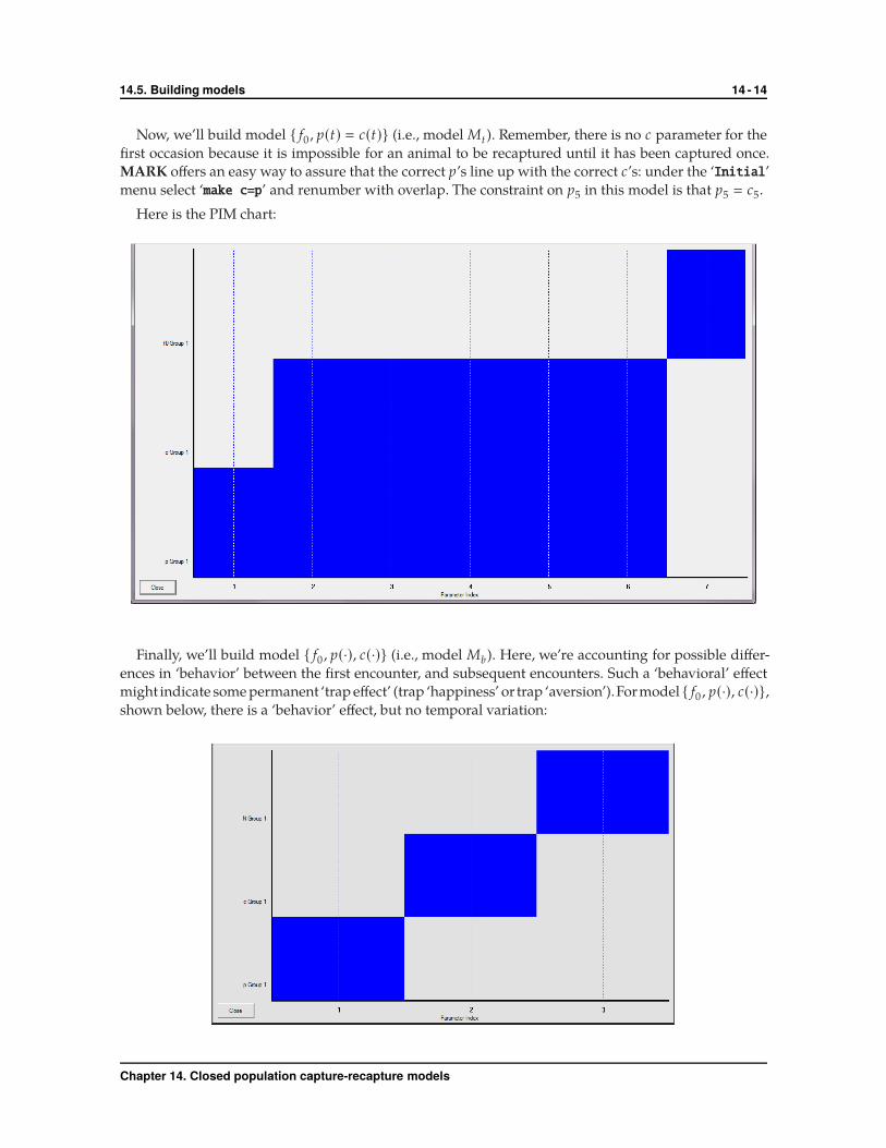
Now, we’ll build model { f0 , p(t) � c(t)} (i.e., model Mt ). Remember, there is no c parameter for the
first occasion because it is impossible for an animal to be recaptured until it has been captured once.
MARK offers an easy way to assure that the correct p’s line up with the correct c’s: under the ‘Initial’
menu select ‘make c=p’ and renumber with overlap. The constraint on p5 in this model is that p5 � c5.
Here is the PIM chart:
Finally, we’ll build model { f0 , p(·), c(·)} (i.e., model Mb). Here, we’re accounting for possible differ-
ences in ‘behavior’ between the first encounter, and subsequent encounters. Such a ‘behavioral’ effect
might indicate some permanent ‘trap effect’ (trap ‘happiness’ or trap ‘aversion’).Formodel { f0 , p(·), c(·)},
shown below, there is a ‘behavior’ effect, but no temporal variation:
Chapter 14. Closed population capture-recapture models
14.6. Closed population models and the design matrix 14 - 15
Note that there is no ‘overlap’ (i.e., no function relating p and c) for this model – this is analogous to
the default model { f0 , p(t), c(t)}, shown earlier. However, in this instance, all parameters are estimable
because of the constraint that p and c are constant over time – the lack of estimability for the final p occurs
if p is time dependent. As such, model { f0 , p(·), c(t)} would be estimable, while model { f0 , p(t), c(·)}
would not (for this model N � Mt+1). You might want to confirm this for yourself.
begin sidebar
simple extension – removal models
Now let’s consider a removal model. These are commonly used in fisheries work where the researcher
does not want to subject a fish to multiple passes of electricity. Therefore, the fish that are encountered
are held aside until all sampling has occurred.
To accomplish this in MARK, build an { f0 , p(t), c(·)} or { f0 , p(·), c(·)} model. Then click ‘Run’ to
open the run window. Click the ‘fix parameters’ button. A window will open listing all of the real
parameters in the model. Simply fix c � 0, and run the model.
Note, however, that a special requirement of removal data is that there has to be a general downward
trend in the number of animals removed on each occasions, i.e., there has to be some depletion of the
population. Seber & Whale (1970) showed that N and p can be estimated from data when the following
“failure criterion” is satisfied:
t∑
j�1
(t + 1 − 2 j)u j > 0,
where t is the number of sampling (removal) occasions, and u j is the number of animals captured and
removed on occasion j.
end sidebar
14.6. Closed population models and the design matrix
In the preceding, we constructed 3 simple models using the PIM chart. While using the PIM chart was
very straightforward for those models, through the design matrix MARK allows models to be fit that
were not possible with the PIM chart. For example, it is possible to build an { f0 , p(t) � c(t) + b} model
where capture probability and recapture probability are allowed to vary through time, but constrained
to be different by an additive constant on the logit scale. It is also worth noting that these extended
models are not available in program CAPTURE (one of several reasons that CAPTURE is no longer
preferred for fitting closed population abundance models).
As introduced in Chapter 6, one approach to doing this is to first build a general model using PIMs,
and then construct the design matrix corresponding to this general model. Then, once you have the
generalmodel constructedusing the design matrix,all othermodels of interest can be constructedsimply
by modifying the design matrix. In this case, the most general model we can build is { f0 , p(t), c(t)}. As
noted earlier, we know before the fact that this particular model is not a useful model, but it is convenient
to build the design matrix for this model as a starting point.
To do this we need the PIMs in the full time varying setup (as shown earlier). Go ahead and run this
model, and add the results to the browser. Look at the real and derived parameter estimates – note that
(i) p5 � 1.0, and (ii) N � Mt+1 � 339. Note as well that the reported SEs for both p5 and N are impossibly
small – a general diagnostic that there is ‘something wrong’ with this model. As discussed earlier, this
is not a useful model without imposing some constraints since the estimate of N � Mt+1.
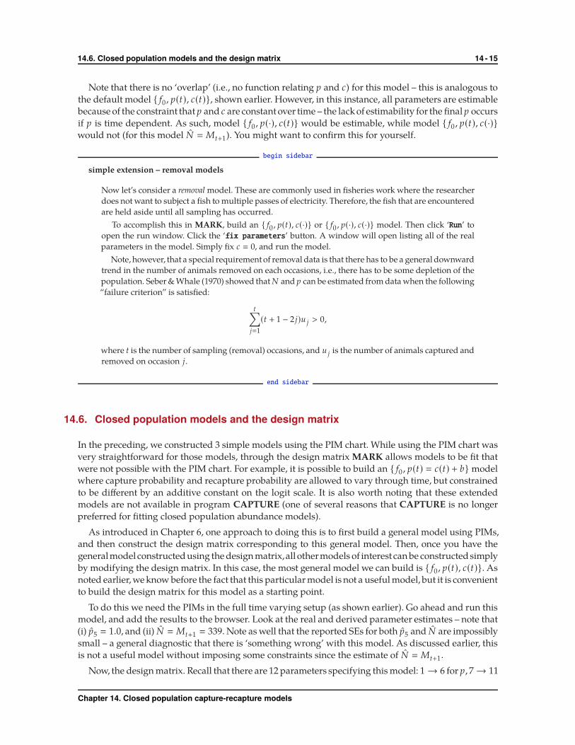
Now, the design matrix. Recall that there are 12 parameters specifying this model: 1 → 6 for p, 7 → 11
Chapter 14. Closed population capture-recapture models
14.6. Closed population models and the design matrix 14 - 16
for c, and parameter 12 for abundance, N . Thus, our design matrix will have 12 columns. Now, if you
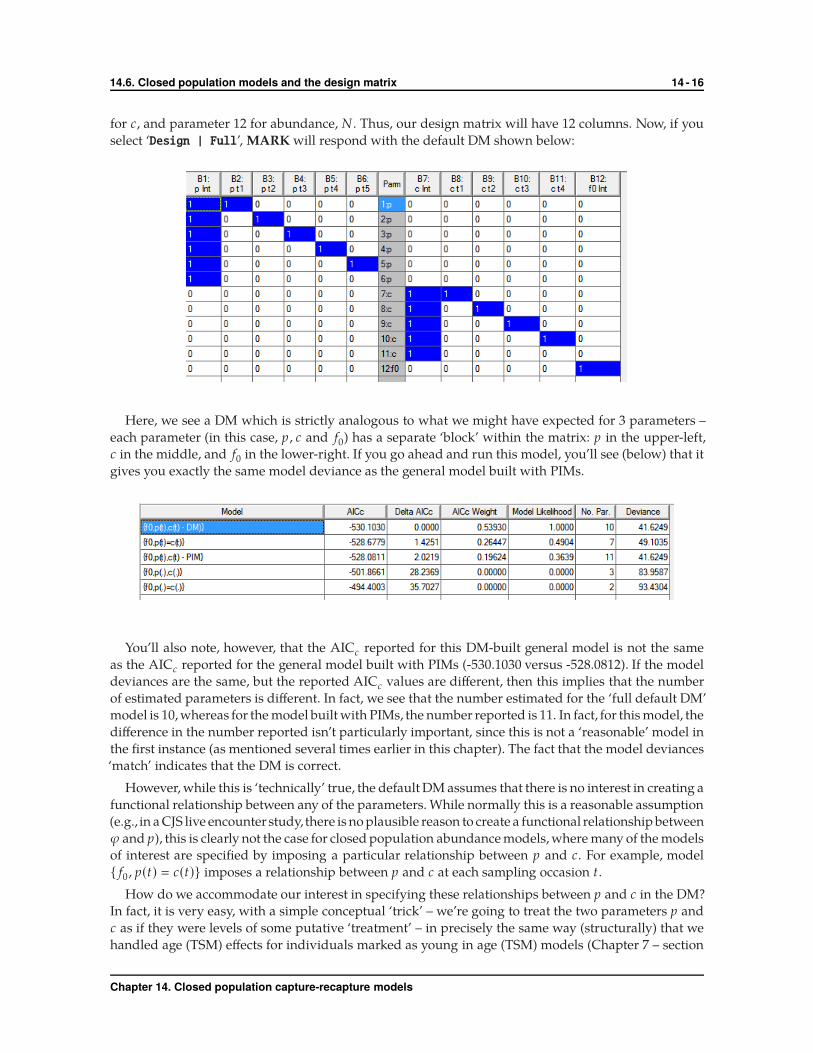
select ‘Design | Full’, MARK will respond with the default DM shown below:
Here, we see a DM which is strictly analogous to what we might have expected for 3 parameters –
each parameter (in this case, p , c and f0) has a separate ‘block’ within the matrix: p in the upper-left,
c in the middle, and f0 in the lower-right. If you go ahead and run this model, you’ll see (below) that it
gives you exactly the same model deviance as the general model built with PIMs.
You’ll also note, however, that the AICc reported for this DM-built general model is not the same
as the AICc reported for the general model built with PIMs (-530.1030 versus -528.0812). If the model
deviances are the same, but the reported AICc values are different, then this implies that the number
of estimated parameters is different. In fact, we see that the number estimated for the ‘full default DM’
model is 10, whereas for the model built with PIMs, the number reported is 11. In fact, for this model, the
difference in the number reported isn’t particularly important, since this is not a ‘reasonable’ model in
the first instance (as mentioned several times earlier in this chapter). The fact that the model deviances
‘match’ indicates that the DM is correct.
However, while this is ‘technically’ true, the default DM assumes that there is no interest in creating a
functional relationship between any of the parameters. While normally this is a reasonable assumption
(e.g., in a CJS live encounter study, there is no plausible reason to create a functional relationship between
ϕ and p), this is clearly not the case for closed population abundance models, where many of the models
of interest are specified by imposing a particular relationship between p and c. For example, model
{ f0 , p(t) � c(t)} imposes a relationship between p and c at each sampling occasion t.
How do we accommodate our interest in specifying these relationships between p and c in the DM?
In fact, it is very easy, with a simple conceptual ‘trick’ – we’re going to treat the two parameters p and
c as if they were levels of some putative ‘treatment’ – in precisely the same way (structurally) that we
handled age (TSM) effects for individuals marked as young in age (TSM) models (Chapter 7 – section
Chapter 14. Closed population capture-recapture models

14.6. Closed population models and the design matrix 14 - 17
7.2). As a reminder, recall how we would construct the design matrix to correspond to the PIM for
survival for a simple age model, with 2 age classes, and time-dependence in each age class. Assume
that we have 7 occasions.
Recall that the PIM for this model looks like:
1 7 8 9 10 11
2 8 9 10 11
3 9 10 11
4 10 11
5 11
6
So, based on the number of indexed parameters in the PIM, we know already that our design matrix
for survival would need to have 11 rows and 11 columns.
What does the linear model look like? Again, writing out the linear model is often the easiest place to
start. In this case we see that over a given time interval, we have, in effect, 2 kinds of individuals: juveniles
(individuals in their first year after marking), and adults (individuals at least 2 years after marking). Thus,
for a given TIME interval, there are 2 groups: juvenile and adult. If we call this group effect AGE, then we
can write out our linear model as
‘survival’ � AGE + TIME + AGE.TIME
� β1
+ β2(AGE)
+ β3(T1) + β4(T2) + β5(T3) + β6(T4) + β7(T5)
+ β8(AGE.T2) + β9(AGE.T3) + β10(AGE.T4) + β11(AGE.T5).
Again, recall from Chapter 7 that there is no (AGE.T1) interaction term. Also remember, we’re treating
the two age classes as different groups – this will be the key ‘conceptual step’ in seeing how we apply
the same idea to closed population abundance models.
The design matrix corresponding to this linear model is:
So, column B2 in this design matrix indicates a putative ‘age group’ – for a given cohort, and a given
time step, is the individual young (indicated with the dummy ‘1’) or adult (indicated with the dummy
Chapter 14. Closed population capture-recapture models
14.6. Closed population models and the design matrix 14 - 18
‘0’). If you don’t recall this connection, go back and re-read section 7.2.
Now, what does this have to do with building design matrices for closed abundance estimation
models? The connection relates to the idea of creating a ‘logical group’. For age models, we used the
age of an individual for a given cohort and time step as a grouping variable. For closed population
abundance models, we do the same thing – except that instead of age, we’re going to ‘group’ as a
function of whether or not the individual has been captured at least once or not. In other words, we’re
going to treat the parameters p (caught for the first time) and c (caught subsequently) as levels of a
putative ‘encounter’ group (analogous to young and adult, respectively).
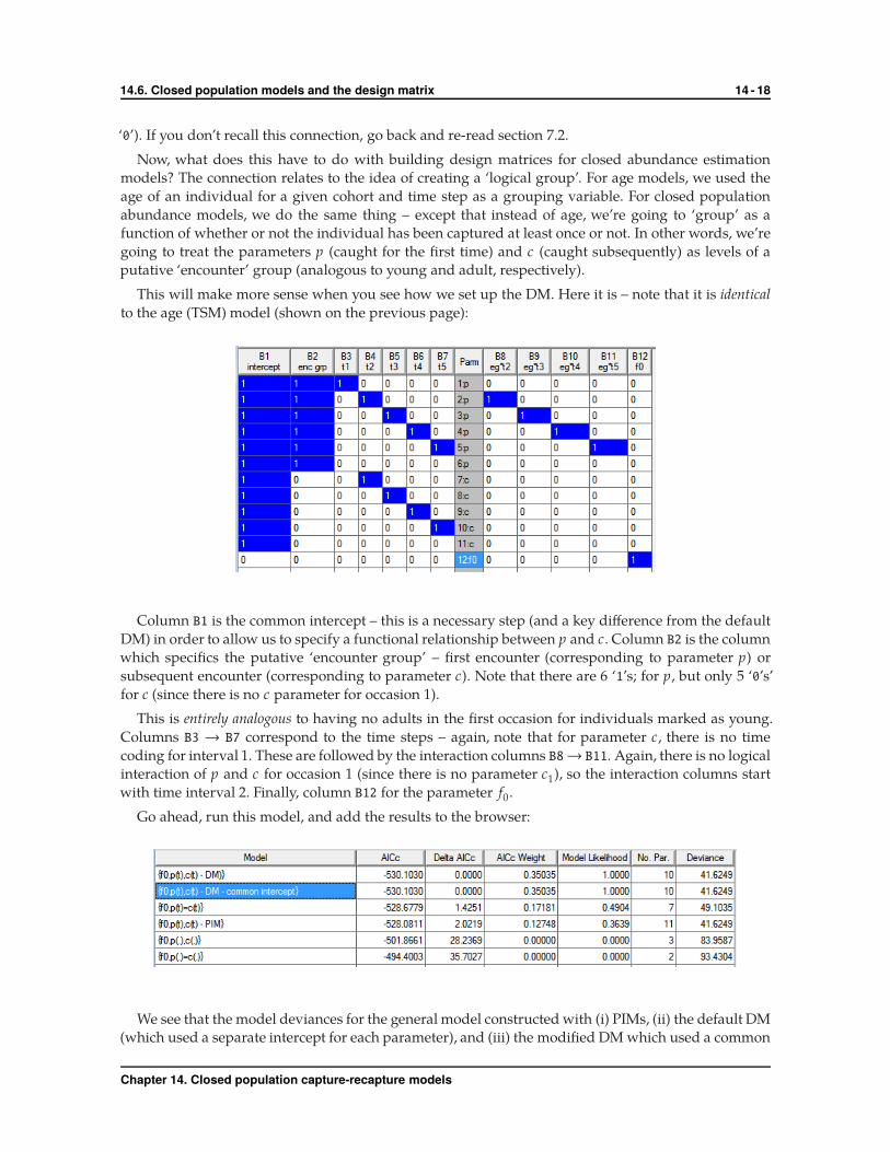
This will make more sense when you see how we set up the DM. Here it is – note that it is identical
to the age (TSM) model (shown on the previous page):
Column B1 is the common intercept – this is a necessary step (and a key difference from the default
DM) in order to allow us to specify a functional relationship between p and c. Column B2 is the column
which specifics the putative ‘encounter group’ – first encounter (corresponding to parameter p) or
subsequent encounter (corresponding to parameter c). Note that there are 6 ‘1’s; for p, but only 5 ‘0’s’
for c (since there is no c parameter for occasion 1).
This is entirely analogous to having no adults in the first occasion for individuals marked as young.
Columns B3 → B7 correspond to the time steps – again, note that for parameter c, there is no time
coding for interval 1. These are followed by the interaction columns B8→ B11. Again, there is no logical
interaction of p and c for occasion 1 (since there is no parameter c1), so the interaction columns start
with time interval 2. Finally, column B12 for the parameter f0.
Go ahead, run this model, and add the results to the browser:
We see that the model deviances for the general model constructed with (i) PIMs, (ii) the default DM
(which used a separate intercept for each parameter), and (iii) the modified DM which used a common
Chapter 14. Closed population capture-recapture models

14.6. Closed population models and the design matrix 14 - 19
intercept, are all identical.
Now, let’s use the DM to build the 3 models we constructed previously using PIMs. First, model
{ f0 , p(·) � c(·)}. We see that (i) there is no temporal variation (meaning, we simply delete the columns
corresponding to time and interactions with time from the DM – columns B3 → B11), and (ii) p � c
(meaning, we delete the column specifying difference between the ‘encounter groups’ – column B2):
Run this model and add the results to the browser:
We see the model results match those of the same model constructed using PIMs.
What about model { f0 , p(·), c(·)}? Here, we again delete all of the time and interaction columns, but
retain the column coding for the ‘encounter group’ term in the model:
Chapter 14. Closed population capture-recapture models

14.6. Closed population models and the design matrix 14 - 20
Again, we see that the results of fitting this model constructed using the DM approach exactly match
those from the same model constructed using PIMs (as indicated on the next page):
Finally, model { f0 , p(t) � c(t)}. Here, we have no ‘encounter group’ effect, but simple temporal
variation in p and c. We simply delete the interaction and ‘encounter group’ columns:
We see (below) that the model deviances are identical, regardless of whether or not the PIM or DM
approach was used.
Now, let’s consider a model which we couldn’t build using the PIM-only approach (or, as noted, if
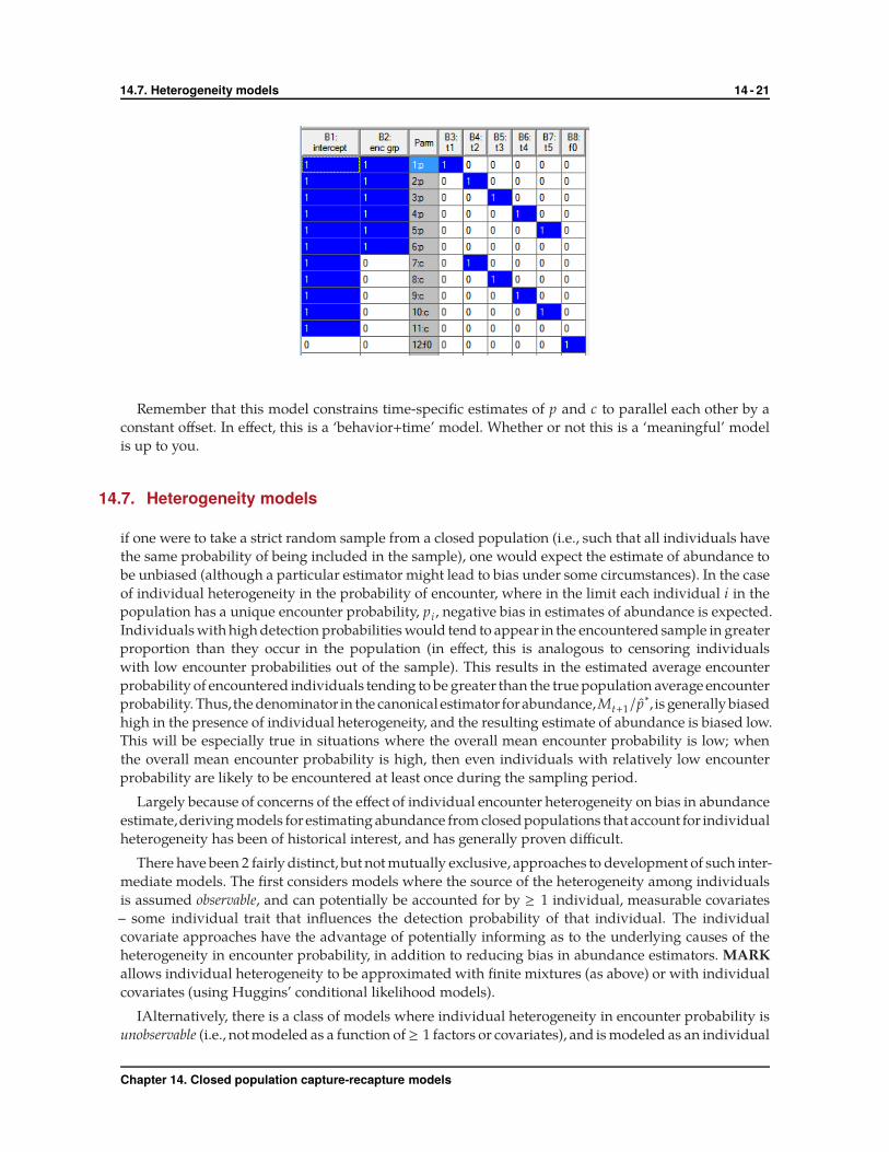
we’d relied on the default DM) – a model with an additive ‘offset’ between p and c. As we introduced
in Chapter 6, to build such additive models, all you need to do is delete the interaction columns from
the DM – this ‘additive’ model is shown at the top of the next page.
Chapter 14. Closed population capture-recapture models
14.7. Heterogeneity models 14 - 21
Remember that this model constrains time-specific estimates of p and c to parallel each other by a
constant offset. In effect, this is a ‘behavior+time’ model. Whether or not this is a ‘meaningful’ model
is up to you.
14.7. Heterogeneity models
if one were to take a strict random sample from a closed population (i.e., such that all individuals have
the same probability of being included in the sample), one would expect the estimate of abundance to
be unbiased (although a particular estimator might lead to bias under some circumstances). In the case
of individual heterogeneity in the probability of encounter, where in the limit each individual i in the
population has a unique encounter probability, pi , negative bias in estimates of abundance is expected.
Individuals with high detection probabilities would tend to appear in the encountered sample in greater
proportion than they occur in the population (in effect, this is analogous to censoring individuals
with low encounter probabilities out of the sample). This results in the estimated average encounter
probability of encountered individuals tending to be greater than the true population average encounter
probability. Thus,the denominator in the canonical estimator forabundance,Mt+1/p∗, is generally biased
high in the presence of individual heterogeneity, and the resulting estimate of abundance is biased low.
This will be especially true in situations where the overall mean encounter probability is low; when
the overall mean encounter probability is high, then even individuals with relatively low encounter
probability are likely to be encountered at least once during the sampling period.
Largely because of concerns of the effect of individual encounter heterogeneity on bias in abundance
estimate,deriving models forestimating abundance from closed populations that account for individual
heterogeneity has been of historical interest, and has generally proven difficult.
There have been 2 fairly distinct, but not mutually exclusive, approaches to development of such inter-
mediate models. The first considers models where the source of the heterogeneity among individuals
is assumed observable, and can potentially be accounted for by ≥ 1 individual, measurable covariates
– some individual trait that influences the detection probability of that individual. The individual
covariate approaches have the advantage of potentially informing as to the underlying causes of the
heterogeneity in encounter probability, in addition to reducing bias in abundance estimators. MARK
allows individual heterogeneity to be approximated with finite mixtures (as above) or with individual
covariates (using Huggins’ conditional likelihood models).
IAlternatively, there is a class of models where individual heterogeneity in encounter probability is
unobservable (i.e., not modeled as a function of ≥ 1 factors or covariates), and is modeled as an individual
Chapter 14. Closed population capture-recapture models
14.7. Heterogeneity models 14 - 22
random effect. Such models are very general because they do not require specification of the possible
source(s) of the heterogeneity. Instead, they posit a parametric probability distribution for {pi} (i.e., the
set {pi} is a random sample of size N drawn from some probability distribution), and use appropriate
methods of parametric inference.
Such unobservable heterogeneity models can be broadly classified in terms of whether the distri-
bution of individuals is modeled as either a discrete- or continuous-mixture, where the population is
implicitly a mixture of individuals with different probabilities of encounter. Norris & Pollock (1996)
and Pledger (2000, 2005) proposed discrete-mixture models where each individual pi may belong to
one of a discrete set of classes (reviewed by Pledger & Phillpot 2008); because the discrete set of classes is
finite, these models are often referred to as finite-mixture models. Alternatively, the mixture distribution
can be continuous infinite (Dorazio & Royle 2003). A commonly used distribution is the logit-normal,
where individuals pi are drawn from a normal distribution (on the logit scale) with specified mean µ
and variance σ2, that is, logit(pi) ∼ N(µ, σ2).
MARK allows you to fit a class of models which are parameterized based on what are known as
‘finite mixtures’. In these models,
pi �
{pi ,A with Pr(π)
pi ,B with Pr(1 − π),
for the case with two mixtures A and B, although the model can be extended to >2 mixtures. As written
(above), the parameter π is the probability that the individual occurs in mixture A. For >2 mixtures,
additional π parameters must be defined (i.e., πA , πB ,...), but constrained to sum to 1.∗ In practice,
most data sets generally support no more than 2 mixtures. Note that the π parameter is assumed to be
constant over time (i.e., an individual in a given mixture is always in that particular mixture over the
sampling period). This has important implications for constructing the DM, which we discuss later.
Alternatively, MARK also allows the fitting of a continuous mixture, based on the logit-normal,
using numerical integration of individual heterogeneity (modeled as a random effect), using Gaussian-
Hermite quadrature. As discussed by Gimenez & Choquet (2010), integration by Gaussian-Hermite
quadrature is very robust under the assumption that the random effect is Gaussian (or nearly so),
and computationally is much more efficient than approaches based on Monte Carlo (MCMC) sam-
pling. Further, because Gaussian-Hermite integration can be embedded in a classical likelihood-based
modeling framework, we can use established methods for goodness-of- fit testing and model selection
to evaluate the relative performance of different heterogeneity models in estimating abundance from
closed population encounter data (White & Cooch 2017).
Here, we introduce both the discrete- and continuous-mixture approaches, as applied to closed
population abundance estimation.† Althoughit remains to be determinedhow well this approachwould
work if the distribution of encounter rates was strongly asymmetric, the underlying model of normally
distributed individual random effects on the logit scale for p provides a more realistic biological model
of heterogeneity than discrete-mixture models when individual heterogeneity is thought to occur over a
continuous scale rather than a discrete set of mixtures. There are clearly cases, however, where the main
source of individual heterogeneity might be better modeled assuming discrete classes (say, in cases
where the main source of difference in encounter probability is an underlying discrete attribute, which
may not be observable; e.g., sex, in cases where the sex of the organism is not observable given the data).
Our purpose here isn’t to fully compare and contrast the two approaches in terms of relative bias and
∗ In practice, this means that you should use the multinomial logit link function, MLogit, to ensure that the estimates do sum to1. The MLogit link was introduced in Chapter 10.
† In fact, ‘finite mixture models’ and ‘individual random effects’ models (based on Gaussian-Hermite quadrature) are availablefor a number of additional data types in MARK – see the Addendum to this chapter.
Chapter 14. Closed population capture-recapture models

14.7.1. Finite, discrete mixture models 14 - 23
precision – it is more than likely that the performance of the two models will differ depending on the
underlying distribution of the heterogeneity (which, of course, is not known). Instead, we focus on the
mechanics of the two approaches in MARK.
14.7.1. Finite, discrete mixture models
Before we demonstrate the ‘mechanics’ of fitting finite mixture models to the data, let’s first consider
the encounter histories (there are 2k possible encounter histories for a k-occasion study), and their
probabilities, for a 4-occasion case for the ‘Full likelihood p and c’ data type:
history cell probability
1000 p1(1 − c2)(1 − c3)(1 − c4)
0100 (1 − p1)p2(1 − c3)(1 − c4)
0010 (1 − p1)(1 − p2)p3(1 − c4)
0001 (1 − p1)(1 − p2)(1 − p3)p4
1100 p1c2(1 − c3)(1 − c4)
1010 p1(1 − c2)c3(1 − c4)
1001 p1(1 − c2)(1 − c3)c4
1110 p1c2c3(1 − c4)
history cell probability
1101 p1c2(1 − c3)c4
1011 p1(1 − c2)c3c4
0110 (1 − p1)p2c3(1 − c4)
0101 (1 − p1)p2(1 − c3)c4
0011 (1 − p1)(1 − p2)p3c4
0111 (1 − p1)p2c3c4
1111 p1c2c3c4
0000 (1 − p1)(1 − p2)(1 − p3)(1 − p4)
If we want to add a finite mixture to the cell probability (i.e., for ‘Full Likelihood Heterogeneity
with pi, p, and c’ data type, with two mixtures), we modify the probability expressions as follows:
history cell probability
1000∑2
a�1
(πa pa1(1 − ca2)(1 − ca3)(1 − ca4)
)
0100∑2
a�1
(πa(1 − pa1)pa2(1 − ca3)(1 − ca4)
)
0010∑2
a�1
(πa(1 − pa1)(1 − pa2)pa3(1 − ca4)
)
0001∑2
a�1
(πa(1 − pa1)(1 − pa2)(1 − pa3)pa4
)
1100∑2
a�1
(πa pa1ca2(1 − ca3)(1 − ca4)
)
1010∑2
a�1
(πa pa1(1 − ca2)ca3(1 − ca4)
)
......
Note: the finite mixture models have a separate set of p’s and c’s for each mixture.
We will demonstrate the fitting of finite mixture (‘heterogeneity’) models to a new sample data set
(mixed_closed1.inp). These data were simulated assuming a finite mixture (i.e., heterogeneity) using
the generating model { f0 , π, p(·) � c(·) � constant} – 9 occasions, 2 mixtures, N � 2,000, π � 0.40, and
pπA� 0.25, pπB
� 0.75. In other words, two mixtures, one with an encounter probability of p � 0.25,
the other with an encounter probability of p � 0.75, with the probability of being in the first mixture
π � 0.40.
Start a new project, select the input data file, set the number of occasions to 9, and specify the ‘Full
Likelihood Heterogeneity with pi, p, and c’ data type. Once we’ve selected a closed data type
Chapter 14. Closed population capture-recapture models

14.7.1. Finite, discrete mixture models 14 - 24
with heterogeneity, you’ll see that an option to specify the number of mixtures is now available in the
‘specification window’ (lower-right side). We’ll use 2 mixtures for this example.
Once you have specified the number of mixtures, open the PIM chart for this data type (when you
switch data types, the underlying model will default to a general time-specific model):
Notice that there are twice as many p’s and c’s as you might have expected given there are 9 occasions
represented in the data. This increase represents the parameters for each of the two mixture groups.
The PIM for the p’s now has two rows defaulting to parameters 2 → 10 and 11 → 19.
Parameters 2 → 10 represent the p’s for the first mixture, and 11 → 19 the p’s for the second mixture.
It becomes more important with the mixture models to keep track of which occasion each c corresponds
to because now both parameter 2 and 11 relate to occasion 1 which has no corresponding c parameter.
We’ll follow the approach used in the preceding section, by first fitting a general model based on
PIMs to the data. You might consider model { f0 , π, p(t), c(t)} as a reasonable starting model. However,
there are two problems with using this as a general, starting model. First, you’ll recall that there are
estimation problems (in general) for a closed abundance model where both p and c are fully time-
dependent. Normally, we need to impose some sort of constraint to achieve identifiability. However,
even if we do so, there is an additional, more subtle problem here – recall we are fitting a heterogeneity
‘mixture’ model, where the parameter π is assumed to be constant over time. As such, there is no
interaction among mixture groups possible over time. Such an interaction would imply time-varying
π. Thus, the most general meaningful model we could fit would be an additive model, with additivity
between the mixture groups, and interaction of p and c within a given mixture group. Recall that we
can’t construct this model using PIMs – building an additive model requires use of the design matrix.
We see from the PIM chart (shown at the top of this page) that the default model structure has 36
Chapter 14. Closed population capture-recapture models
14.7.1. Finite, discrete mixture models 14 - 25
columns. Note: if you select ’Design | Full’, MARK will respond with an error message, telling you it
can’t build a default fully time-dependent DM. Basically, for heterogeneity models, you’ll need to build
the DM by hand – meaning, starting with a reduced DM. So, we select ‘Design | Reduced’, and keep
the default 36 columns.
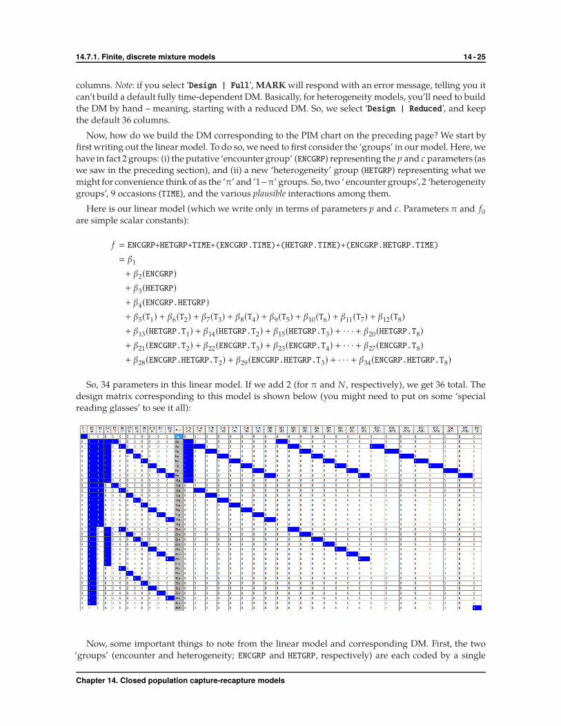
Now, how do we build the DM corresponding to the PIM chart on the preceding page? We start by
first writing out the linear model. To do so, we need to first consider the ‘groups’ in our model. Here, we
have in fact 2 groups: (i) the putative ‘encounter group’ (ENCGRP) representing the p and c parameters (as
we saw in the preceding section), and (ii) a new ‘heterogeneity’ group (HETGRP) representing what we
might for convenience think of as the ‘π’ and ‘1−π’ groups. So, two ‘ encounter groups’, 2 ‘heterogeneity
groups’, 9 occasions (TIME), and the various plausible interactions among them.
Here is our linear model (which we write only in terms of parameters p and c. Parameters π and f0are simple scalar constants):
f � ENCGRP+HETGRP+TIME+(ENCGRP.TIME)+(HETGRP.TIME)+(ENCGRP.HETGRP.TIME)
� β1
+ β2(ENCGRP)
+ β3(HETGRP)
+ β4(ENCGRP.HETGRP)
+ β5(T1) + β6(T2) + β7(T3) + β8(T4) + β9(T5) + β10(T6) + β11(T7) + β12(T8)
+ β13(HETGRP.T1) + β14(HETGRP.T2) + β15(HETGRP.T3) + · · · + β20(HETGRP.T8)
+ β21(ENCGRP.T2) + β22(ENCGRP.T3) + β23(ENCGRP.T4) + · · · + β27(ENCGRP.T8)
+ β28(ENCGRP.HETGRP.T2) + β29(ENCGRP.HETGRP.T3) + · · · + β34(ENCGRP.HETGRP.T8)
So, 34 parameters in this linear model. If we add 2 (for π and N , respectively), we get 36 total. The
design matrix corresponding to this model is shown below (you might need to put on some ‘special
reading glasses’ to see it all):
Now, some important things to note from the linear model and corresponding DM. First, the two
‘groups’ (encounter and heterogeneity; ENCGRP and HETGRP, respectively) are each coded by a single
Chapter 14. Closed population capture-recapture models
14.7.1. Finite, discrete mixture models 14 - 26
column (single β) – columns B3 for ENCGRP and B4 for HETGRP. 9 sampling occasions, so 8 columns for
time (B5→ B12). The remaining columns code for the two-way interactions between ENCGRP (E),HETGRP
(H) and time (T), and the three-way interaction (H.E.Tx).
Now, if you run this model constructed using the DM, , you’ll se that the model deviance is identical
to the model constructed using PIMs (indicating that our DM is correct). However, if you look at
the parameter estimates, you’ll quickly notice that, as expected, quite a few of the parameters aren’t
identifiable. In particular, the final p estimates for the two mixture groups have problems, and the
derived estimate of N is simply Mt+1 (the SE of the abundance estimate is clearly wrong).
Why the problems? Simple – despite the fact we have 2 mixture groups, this is still model {p(t), c(t)},
which we know is not identifiable – and thus, is not a useful model to fit to the data – without constraints.
One possible constraint is to model p and c as additive functions of each other. How can we modify the
DM to apply this constraint?
Simple – by eliminating the interactions between ENCGRP and TIME. In other words, deleting columns
B14→ B20 (coding for the interaction of ENCGRP and TIME), and columns B29→ B35 (coding for the 3-way
interaction of HETGRP, ENCGRP, and TIME) from the DM shown on the previous page. This model allows
time variation, behavioral variation and individual heterogeneity in capture probability, yet does so in
an efficient and parsimonious (and estimable) manner.
We can use this DM to create additional, reduced parameter models. For example, we could build
model { f0 , pa(t) � ca(t) � pb(t) + z � cb(t) + z } representing capture probability varying through time
and additive difference between mixture groups, but with no interaction between p and c over time (no
behavior effect). We do this simply by deleting the ENCGRP column from the DM.
As a final test – how do we modify the DM to match the true generating model, which for these data
was model { f0 , π, pA � cA , pB � cB}? To build this model from our DM, we simply delete (i) all the
time columns, (ii) any interactions with time, and (iii) the encounter group column (ENCGRP). We delete
the encounter group column because we’re setting p � c. We retain the heterogeneity (mixture) group
column (HETGRP) since we want to allow for the possibility that encounter probability differs between
mixtures (which of course is logically necessary for a mixture model!).
Both the real and derived parameter estimates (π � 0.607, pπA� 0.250, pπB
� 0.754, N � 1,995.494)
are quite close to the true parameter values used in the generating model. [But, what about π? The true
value we used in the simulation wasπ � 0.40. The estimated value π � 0.607 is simply the complement.]
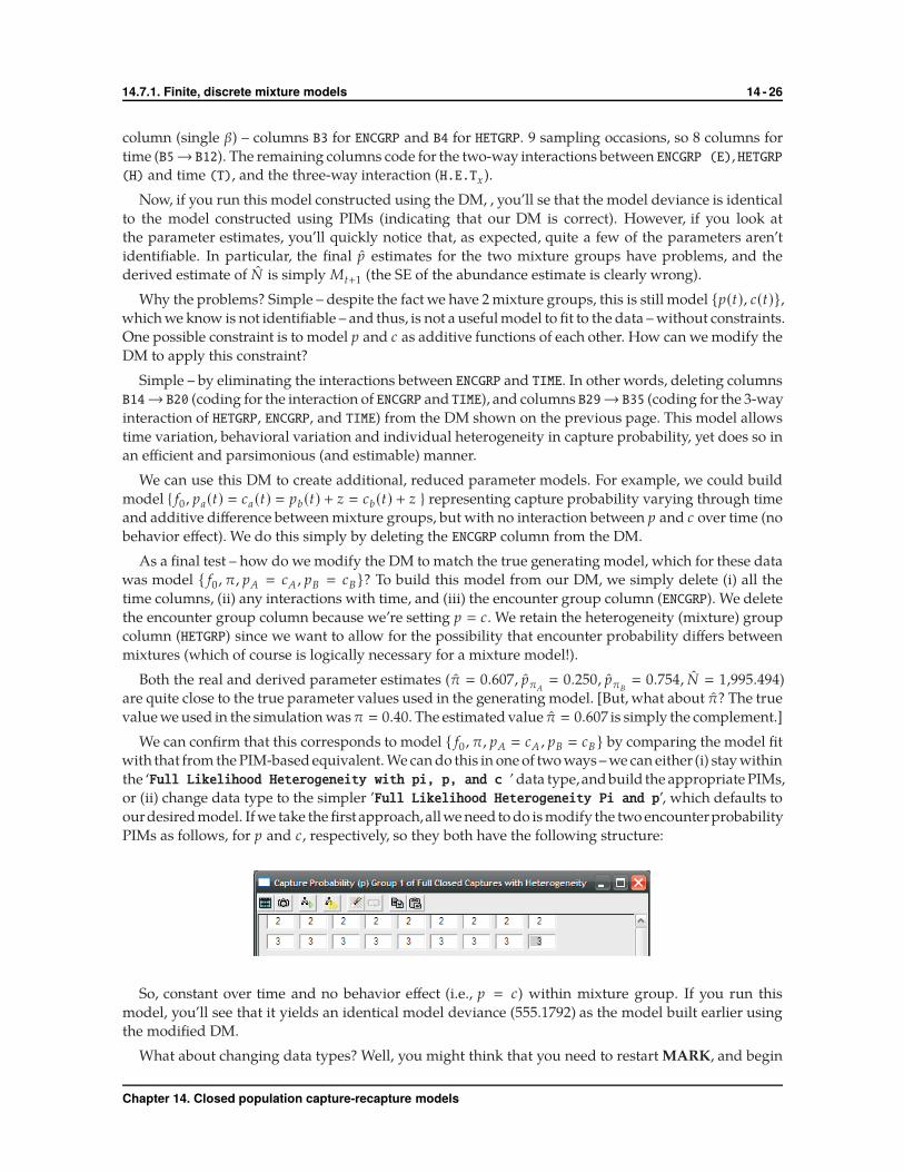
We can confirm that this corresponds to model { f0 , π, pA � cA , pB � cB} by comparing the model fit
with that from the PIM-based equivalent. We can do this in one of two ways – we can either (i) stay within
the ‘Full Likelihood Heterogeneity with pi, p, and c ’ data type,andbuild the appropriate PIMs,
or (ii) change data type to the simpler ’Full Likelihood Heterogeneity Pi and p’, which defaults to
ourdesiredmodel. Ifwe take the firstapproach,allwe need to do is modify the two encounterprobability
PIMs as follows, for p and c, respectively, so they both have the following structure:
So, constant over time and no behavior effect (i.e., p � c) within mixture group. If you run this
model, you’ll see that it yields an identical model deviance (555.1792) as the model built earlier using
the modified DM.
What about changing data types? Well, you might think that you need to restart MARK, and begin
Chapter 14. Closed population capture-recapture models
14.7.2. Continuous mixture models using numerical integration 14 - 27
a new project after first specifying the new data type. In fact, you don’t need to – you can simply ‘tell’
MARK that you want to switch data types (something MARK lets you do within certain types of models
– in this instance, closed population abundance estimators). All you need to do is select ‘PIM | change
data type’ on the main menu bar, and then select ‘Full Likelihood Heterogeneity Pi and p’ from
the resulting popup window. As noted earlier, the default model for this data type is the model we’re
after – it is simply a reduced parameter version of the full model.
Interpreting π from finite mixture models
So, you do an analysis using a closed population heterogeneity abundance model, based on finite
mixtures, and derive an estimate of π. Perhaps you’ve built several such models, and have a model
averaged estimate of ¯π. So, what do you ‘say’ about this estimate of π?
Easy answer – generally nothing. The estimate of π is based on fitting a finite mixture model, with a
(typically small) number of discrete states. When we simulated such data (above), we used a discrete
simulation approach – we simply imagined a population where 40% of the individuals had one
particular detection probability, and 60% had a different encounter probability. In that case, because
the distribution of individuals in the simulated population was in fact discrete, then the real estimate
of π reflected the true generating parameter.
However, if in fact the variation in detection probability was (say) continuous, then in fact the estimate
of π reflects a ‘best estimate’ as to where a discrete ‘breakpoint’ might be (breaking the data into a set
of discrete, finite mixtures). Such an estimate is not interpretable, by and large. Our general advice is
to avoid post hoc story-telling with respect to π, no matter how tempting (or satisfying) the story might
seem.
14.7.2. Continuous mixture models using numerical integration
Now, we’ll consider models where we assume that the individual heterogeneity is continuous logit-
normal. The basic ideas underlying continuous mixture models are relatively simple. First, we assume
a population where individual encounter probabilities were randomly drawn from a logit-normal
distribution, specified by a known µp and σ2p . The continuous mixture model is implemented in MARK
for using the Huggins estimator, extended by including an individual random effect for the encounter
probability (pik) of each individual i constant across occasions k � 1, . . . , t on the logit scale following
McClintock et al. (2009) (see also Chapter 18), Gimenez & Choquet (2010), and White & Cooch (2017):
logit(pik) � βk + ǫi ,
with βk a fixed effect modeling time, and ǫi a normally distributed random effect with mean zero and
unknown variance σ2p . Hence
pik �1
1 + exp(−(βk + σpZi)),
where Zi ∼ N(0., 1). Therefore, individual i on occasion k has the probability of being encountered
pik �
∫+∞
−∞
1
1 + exp(−(βk + σp Zi)
) ϕ(Zi)dZi ,
where ϕ(Zi) is the probability density function of the standard normal distribution. The estimate of
Chapter 14. Closed population capture-recapture models
14.7.2. Continuous mixture models using numerical integration 14 - 28
population abundance, N , is obtained following Huggins (1989) as the summation across animals
encountered ≥ 1 time,
N �
Mt+1∑
i�1
(1
p∗i
),
where
p∗i � 1 −
∫+∞
−∞
k∏
i�1
(1 −
1
1 + exp(−(βk + σpZi)
))ϕ(Zi)dZi .
Because this integral does not have a closed form, the likelihood must be integrated numerically
– in program MARK, this is accomplished using Gaussian-Hermite quadrature (McClintock et al. 2009,
Gimenez & Choquet 2010, White & Cooch 2017).
To demonstrate the mechanics, we’ll start with the same simulated data set we used in the preceding
section where we introduced discrete-mixtures (mixed_closed1.inp). Recall that these encounter data
were simulated using the generating model { f0 , π, p(·) � c(·)} – 9 occasions, 2 mixtures, N � 2,000,
π � 0.40, and pπA� 0.25, pπB
� 0.75. In other words, the data do in fact consist of two discrete classes
of individuals, one with an encounter probability of p � 0.25, the other with an encounter probability
of p � 0.75, with the probability of being in the first mixture π � 0.40. With a bit of thought, you should
realize that this data set is not symmetrical around some ‘mean’ encounter probability.
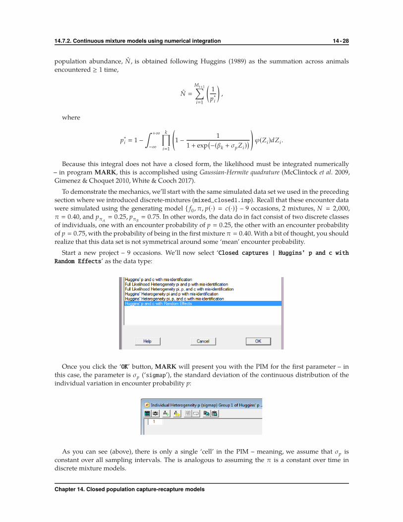
Start a new project – 9 occasions. We’ll now select ‘Closed captures | Huggins’ p and c with
Random Effects’ as the data type:
Once you click the ‘OK’ button, MARK will present you with the PIM for the first parameter – in
this case, the parameter is σp (‘sigmap’), the standard deviation of the continuous distribution of the
individual variation in encounter probability p:
As you can see (above), there is only a single ‘cell’ in the PIM – meaning, we assume that σp is
constant over all sampling intervals. The is analogous to assuming the π is a constant over time in
discrete mixture models.
Chapter 14. Closed population capture-recapture models
14.7.2. Continuous mixture models using numerical integration 14 - 29
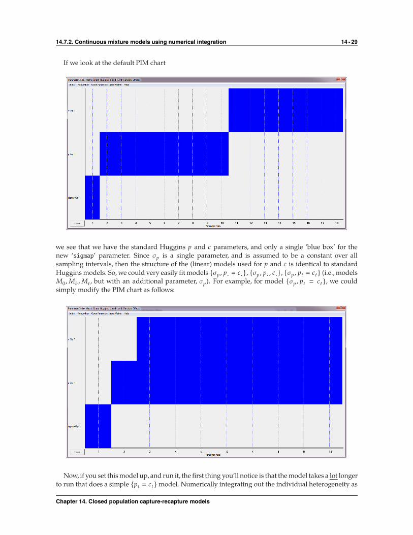
If we look at the default PIM chart
we see that we have the standard Huggins p and c parameters, and only a single ‘blue box’ for the
new ‘sigmap’ parameter. Since σp is a single parameter, and is assumed to be a constant over all
sampling intervals, then the structure of the (linear) models used for p and c is identical to standard
Huggins models. So, we could very easily fit models {σp , p· � c·}, {σp , p· , c·}, {σp , pt � ct} (i.e., models
M0 ,Mb ,Mt , but with an additional parameter, σp). For example, for model {σp , pt � ct }, we could
simply modify the PIM chart as follows:
Now, if you set this model up, and run it, the first thing you’ll notice is that the model takes a lot longer
to run that does a simple {pt � ct } model. Numerically integrating out the individual heterogeneity as
Chapter 14. Closed population capture-recapture models
14.7.2. Continuous mixture models using numerical integration 14 - 30
an individual random effect takes some computation time.
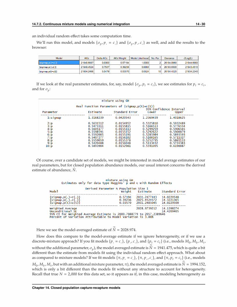
We’ll run this model, and models {σp , p· � c·} and {σp , p· , c·} as well, and add the results to the
browser:
If we look at the real parameter estimates, for, say, model {σp , pt � ct}, we see estimates for pt � ct ,
and for σp :
Of course, over a candidate set of models, we might be interested in model average estimates of our
real parameters, but for closed population abundance models, our usual interest concerns the derived
estimate of abundance, N .
Here we see the model-averaged estimate of N � 2028.974.
How does this compare to the model-average estimate if we ignore heterogeneity, or if we use a
discrete-mixture approach? If you fit models {p· � c·}, {p· , c·}, and {pt � ct } (i.e., models M0 ,Mb ,Mt ,
without the additional parameter, σp), the model averaged estimate is N � 1941.475,which is quite a bit
different than the estimate from models fit using the individual random effect approach. What about
as compared to mixture models? If we fit models {π, p· � c·}, {π, p· , c·}, and {π, pt � ct} (i.e., models
M0 ,Mb ,Mt , but with an additional mixture parameter,π), the model averaged estimate is N � 1994.152,
which is only a bit different than the models fit without any structure to account for heterogeneity.
Recall that true N � 2,000 for this data set, so it appears as if, in this case, modeling heterogeneity as
Chapter 14. Closed population capture-recapture models
14.7.2. Continuous mixture models using numerical integration 14 - 31
an individual random effect has performed a bit less well than either using finite mixtures, or ignoring
the heterogeneity altogether (although, clearly, we haven’t done an exhaustive analysis of these data).
To emphasize the fact that results of using different approaches to heterogeneity can be ‘twitchy’
(from the Latin), here are some summary results from a large series of simulations (1,000) with true
N � 100, σp � 1.0, preal � 0.35, k � 5 occasions, where the encounter data were generated under true
model M0,RE (i.e., p· � c·, with logit-normal variation in pi for each individual i). To these simulated
data, we fit 3 models to the data: {p· � c·}, {σp , p· � c·}, and {π, p· � c·}.
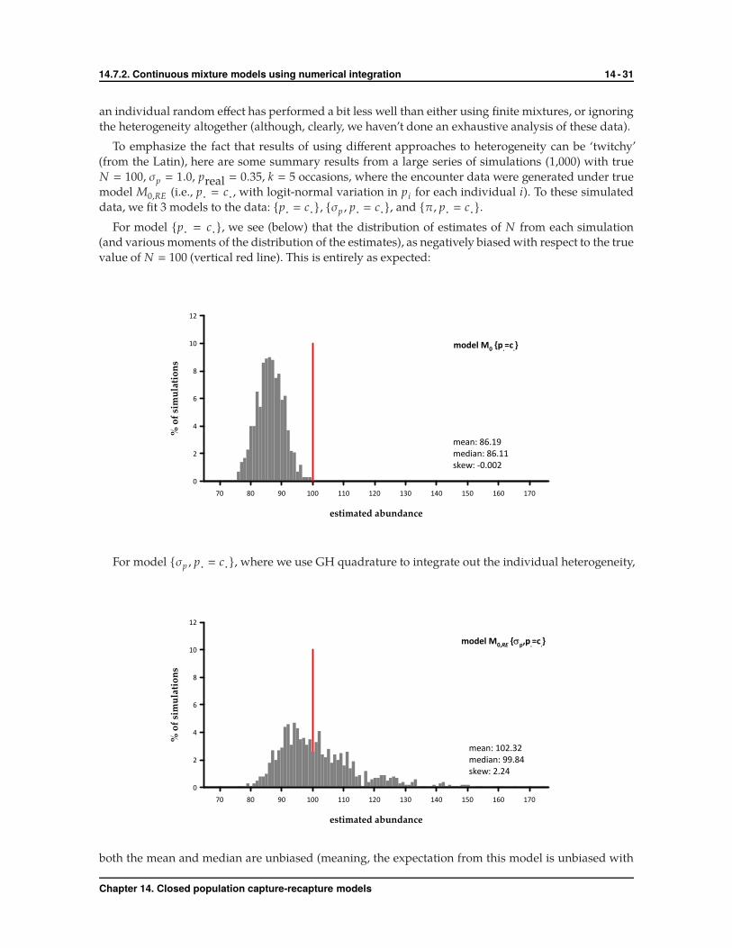
For model {p· � c·}, we see (below) that the distribution of estimates of N from each simulation
(and various moments of the distribution of the estimates), as negatively biased with respect to the true
value of N � 100 (vertical red line). This is entirely as expected:
�����������������
�� �� �� ��� ��� ��� �� �� ��� ��� ���
��������������
�
�
�
�
��
��
�����������
�������������
������������
���������
��
��
For model {σp , p· � c·}, where we use GH quadrature to integrate out the individual heterogeneity,
�����������������
�� �� �� ��� ��� ��� �� �� ��� ��� ���
��������������
�
�
�
�
��
��
�����������
������������
���������
����������
����
� �
��
both the mean and median are unbiased (meaning, the expectation from this model is unbiased with
Chapter 14. Closed population capture-recapture models
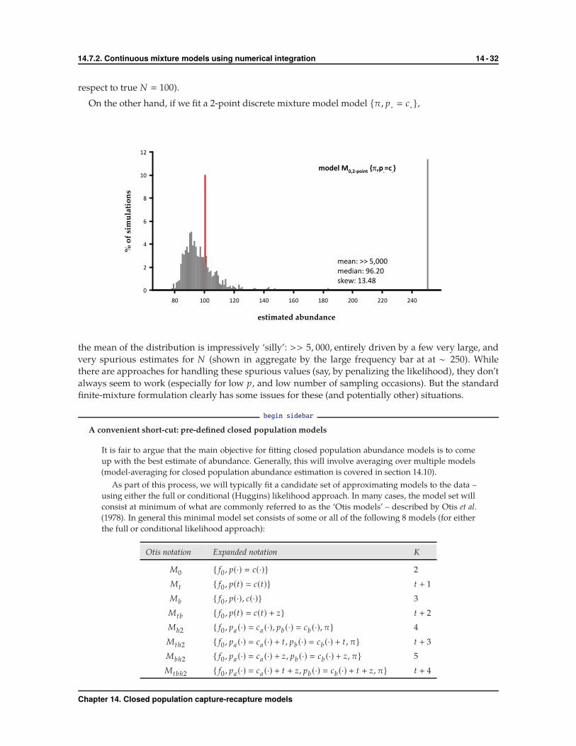
14.7.2. Continuous mixture models using numerical integration 14 - 32
respect to true N � 100).
On the other hand, if we fit a 2-point discrete mixture model model {π, p· � c·},
�����������������
�� ��� ��� ��� ��� ��� ��� ��� ���
��������������
�
�
�
�
�
��
��
�� ����������
���� �������
�����������
����������� ��
�������
��
the mean of the distribution is impressively ‘silly’: >> 5, 000, entirely driven by a few very large, and
very spurious estimates for N (shown in aggregate by the large frequency bar at at ∼ 250). While
there are approaches for handling these spurious values (say, by penalizing the likelihood), they don’t
always seem to work (especially for low p, and low number of sampling occasions). But the standard
finite-mixture formulation clearly has some issues for these (and potentially other) situations.
begin sidebar
A convenient short-cut: pre-defined closed population models
It is fair to argue that the main objective for fitting closed population abundance models is to come
up with the best estimate of abundance. Generally, this will involve averaging over multiple models
(model-averaging for closed population abundance estimation is covered in section 14.10).
As part of this process, we will typically fit a candidate set of approximating models to the data –
using either the full or conditional (Huggins) likelihood approach. In many cases, the model set will
consist at minimum of what are commonly referred to as the ‘Otis models’ – described by Otis et al.
(1978). In general this minimal model set consists of some or all of the following 8 models (for either
the full or conditional likelihood approach):
Otis notation Expanded notation K
M0 { f0 , p(·) � c(·)} 2
Mt { f0 , p(t) � c(t)} t + 1
Mb { f0 , p(·), c(·)} 3
Mtb { f0 , p(t) � c(t) + z} t + 2
Mh2 { f0 , pa (·) � ca (·), pb (·) � cb (·), π} 4
Mth2 { f0 , pa (·) � ca (·) + t , pb (·) � cb (·) + t , π} t + 3
Mbh2 { f0 , pa (·) � ca (·) + z, pb (·) � cb (·) + z, π} 5
Mtbh2 { f0 , pa (·) � ca (·) + t + z, pb (·) � cb (·) + t + z, π} t + 4
Chapter 14. Closed population capture-recapture models
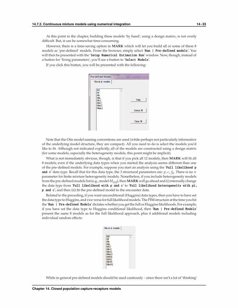
14.7.2. Continuous mixture models using numerical integration 14 - 33
At this point in the chapter, building these models ‘by hand’, using a design matrix, is not overly
difficult. But, it can be somewhat time-consuming.
However, there is a time-saving option in MARK which will let you build all or some of these 8
models as ‘pre-defined’ models. From the browser, simply select ‘Run | Pre-defined models’. You
will then be presented with the ‘Setup Numerical Estimation Run’ window. Now, though, instead of
a button for ‘fixing parameters’, you’ll see a button to ‘Select Models’.
If you click this button, you will be presented with the following:
Note that the Otis model naming conventions are used (while perhaps not particularly informative
of the underlying model structure, they are compact). All you need to do is select the models you’d
like to fit. Although not indicated explicitly, all of the models are constructed using a design matrix
(for some models, especially the heterogeneity models, this point might be implicit).
What is not immediately obvious, though, is that if you pick all 12 models, then MARK will fit all
8 models, even if the underlying data types when you started the analysis seems different than one
of the pre-defined models. For example, suppose you start an analysis using the ‘Full likelihood p
and c’ data type. Recall that for this data type, the 3 structural parameters are: p, c, f0. There is no π
parameter for finite mixture heterogeneity models. Nonetheless, if you include heterogeneity models
from the pre-defined models list (e.g.,model Mth2), then MARK will go ahead and (i) internally change
the data type from ‘Full likelihood with p and c’ to ‘Full likelihood heterogeneity with pi,
p and c’, and then (ii) fit the pre-defined model to the encounter data.
Related to the preceding, if you want unconditional (Huggins) data types, then you have to have set
the data type to Huggins,andvice versa for full likelihoodmodels.The PIM structure at the time you hit
the ‘Run | Pre-defined Models’ dictates whetheryou get the full orHuggins likelihoods.Forexample,
if you have set the data type to Huggins conditional likelihood, then ‘Run | Pre-defined Models’
present the same 8 models as for the full likelihood approach, plus 4 additional models including
individual random effects:
While in general pre-defined models should be used cautiously – since there isn’t a lot of ‘thinking’
Chapter 14. Closed population capture-recapture models

14.8. Misidentification models 14 - 34
involved with fitting them to the data – being able to build some of the canonical closed population
abundance models with only a few clicks can be a real time-saver.
end sidebar
Closing comment: individual heterogeneity – the bane of abundance estimation
It is perhaps reasonable to speculate that in preceding example, where the underlying heterogeneity
simulated in the data was truly continuous logit-normal, that GH integration will perform particularly
well, better than a finite-mixture approach which models heterogeneity as if there were in fact discrete
‘groups’ of individuals. However, in the absence of strong prior information (or, ‘expectation’) about the
form of the heterogeneity (at the least, continuous versus discrete), it is probably somewhat misleading
to imply that one approach or the the other will be the most robust in modeling heterogeneity.
While the approaches discussed in the preceding can be effective, the single best way to minimize
the bias caused by individual heterogeneity is to get p as high as possible – the ‘big law’ of capture-
recapture design. When p is high there is little room for variation and little chance that an individual
is not detected.
Bill Link (2003, 2004) demonstrated that different models of the form of individual heterogeneity
can lead to very different estimates of abundance and fit the data equally well. The magnitude of the
differences in abundance estimates is related to p; when p is small the differences can be large. Therefore,
to have much hope of estimating abundance with little bias, capture probability must be relatively high.
In addition, the primary issue with using the individual random effects estimator (and likely discrete-
mixture approaches as well) in adequately fitting complex models is obtaining an adequate number of
occasions to be able to estimate σp (or π) with any precision. A lower level of > 5 occasions is likely
necessary to achieve reasonable performance for either the continuous- or discrete-mixture approaches
(White & Cooch 2017).
Individual heterogeneity is a common source of bias, typically causing capture-mark-reencounter
estimates of population abundance to be biased low. Continuous- and finite-mixture models may be an
effective approach to eliminate this bias when an adequate number of capture occasions are available
and detection probabilities are relatively high. To have much hope of estimating abundance with little
bias, we reiterate the ‘big law’ – encounter probability must be relatively high.
In sampling situations with low encounter probabilities (p ≤ 0.2), and a low number of samples
(K ≤ 5), the investigator will need to be aware of the potential for biased estimates, and evaluate
whether not the direction of bias (which reflects the estimator – generally negative for models that
do not account for heterogeneity, and potentially positive for models that do account for heterogeneity)
is important in the applied context. For example, for management of small, threatened populations, the
potential ramifications of under-estimating (negative bias) or over-estimating (positive bias) abundance
are clearly of some importance.
14.8. Misidentification models
The likelihoods and cell probabilities get more complicated when we want to include the possibility
of misidentification into the cell probabilities. In order to do this we must assume that (i) an individual
encountered more than once is correctly identified (i.e., individuals captured on multiple occasions
are correctly identified – owing to the greater amount of information gathered on which to base the
identification), and (ii) individuals encountered only once may or may not be correctly identified.
First, we consider the closed capture cell probabilities without finite mixtures. We will add the
possibility of misidentification (where α is the probability of correctly identifying the individual) to
Chapter 14. Closed population capture-recapture models
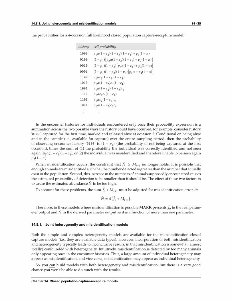
14.8.1. Joint heterogeneity and misidentification models 14 - 35
the probabilities for a 4-occasion full likelihood closed population capture-recapture model:
history cell probability
1000 p1α(1 − c2)(1 − c3)(1 − c4) + p1(1 − α)
0100 (1 − p1)[p2α(1 − c3)(1 − c4) + p2(1 − α)
]
0010 (1 − p1)(1 − p2)[p3α(1 − c4) + p3(1 − α)
]
0001 (1 − p1)(1 − p2)(1 − p3)[p4α + p4(1 − α)
]
1100 p1αc2(1 − c3)(1 − c4)
1010 p1α(1 − c2)c3(1 − c4)
1001 p1α(1 − c2)(1 − c3)c4
1110 p1αc2c3(1 − c4)
1101 p1αc2(1 − c3)c4
1011 p1α(1 − c2)c3c4
......
In the encounter histories for individuals encountered only once their probability expression is a
summation across the two possible ways the history could have occurred; for example, consider history
‘0100’; captured for the first time, marked and released alive at occasion 2. Conditional on being alive
and in the sample (i.e., available for capture) over the entire sampling period, then the probability
of observing encounter history ‘0100’ is(1 − p1
)(the probability of not being captured at the first
occasion), times the sum of (1) the probability the individual was correctly identified and not seen
again (p2α(1 − c3)(1− c4), or (2) the individual was misidentified and therefore unable to be seen again
p2(1 − α).
When misidentification occurs, the constraint that N ≥ Mt+1 no longer holds. It is possible that
enough animals are misidentified such that the number detected is greater than the number that actually
exist in the population. Second, this increase in the numbers of animals supposedly encountered causes
the estimated probability of detection to be smaller than it should be. The effect of these two factors is
to cause the estimated abundance N to be too high.
To account for these problems, the sum f0 + Mt+1 must be adjusted for mis-identification error, α:
N � α(
f0 + Mt+1
).
Therefore, in these models where misidentification is possible MARK presents f0 in the real param-
eter output and N in the derived parameter output as it is a function of more than one parameter.
14.8.1. Joint heterogeneity and misidentification models
Both the simple and complex heterogeneity models are available for the misidentification closed
capture models (i.e., they are available data types). However, incorporation of both misidentification
and heterogeneity typically leads to inconclusive results, in that misidentification is somewhat (almost
totally) confounded with heterogeneity. Intuitively, misidentification is detected by too many animals
only appearing once in the encounter histories. Thus, a large amount of individual heterogeneity may
appear as misidentification, and vice versa, misidentification may appear as individual heterogeneity.
So, you can build models with both heterogeneity and misidentification, but there is a very good
chance you won’t be able to do much with the results.
Chapter 14. Closed population capture-recapture models
14.9. Goodness-of-fit 14 - 36
14.9. Goodness-of-fit
In general, testing model fit in the closed-population capture-recapture models remains an unresolved
issue, even more so than in other capture-recapture model types. A central component of the problem
stems from the fact that there often is no unique way to compute a saturated model. If one was only
concerned about time variation in capture probability, then goodness-of-fit is fairly straightforward.
When individual heterogeneity is added into the problem there is an infinite set of possible models for
heterogeneity. Thus, no unique goodness-of-fit exists.
In past, several tests of model assumptions have been developed for the closed-population capture-
recapture models (Otis et al. 1978: 50-67, White et al. 1982: 77-79). The seven tests examine the fit of
specific model forms relative to other specific models or vague alternatives (i.e., the model fails to
fit for unspecified reasons). These tests are available in MARK through CAPTURE by selecting the
‘Appropriate’ check box in the CAPTURE window. The tests were developed largely as a means of
model selection in the absence of another method. Now that MARK employs AICc as a selection
criterion and that it has been shown the model averaged estimates of N have better properties than
single-model estimates (Stanley and Burnham 1998), the tests of Otis et al. (1978) have fallen out of use.
Recently, David Fletcher has proposed (Fletcher 2012) a new approach which appears to work very
well, at least for models (with or without heterogeneity), based on the Huggins conditional likelihood.
Typically, estimating over- dispersion (c) from the observed number of individuals associated with
each possible encounter history is complicated by the large number of encounter histories with very
low expected frequencies, especially when the average encounter probability is low. Commonly, an
estimate of overdispersion is based on Pearson’s χ2 lack-of-fit statistic. Fletcher (2012) proposed a new
estimator with smaller variance,
c �
cx
r,where r �
1
H
H∑
i�1
yi
ηi
.
Here, cx is the estimator of overdispersion based on the Pearson χ2 statistic (i.e., the Pearson χ2
statistic divided by the degrees of freedom, where σp is included in the parameter count for the random
effects models because it is an estimated parameter – D. J. Fletcher, University of Otago, personal
communication), yi and ηi are the observed and expected number of individuals with encounter history
i, and H � 2t −1 is the number of observable histories over t occasions. One of the problems with using
Pearson’s statistic for sparse data is that the ith term involves dividing by ηi , which will often be very
small. The new estimator makes an allowance for this because the ith term in the denominator also
involves dividing by ηi . Simulations suggest that this new estimator also performs better than those
based on the deviance.
White & Cooch (2017) showed that the Fletcher c showed very good potential to detect individual
heterogeneity, which would generally be of some importance in the context of abundance estimation.
There are a couple of issues which you need to take into account in applying this approach. First, losses
on capture or dots in the encounter history will create encounter histories that are not considered in the
total number of possible encounter histories. That is, the total number of possible encounter histories
is based on no missing data. Second, parameter values that cause a reduction in the total number of
encounter histories will bias the c estimate. Examples of such reductions are an occasion with p � 0, or
transition probabilities fixed to 0 or 1 in the multi-state data types.
For application of the Fletcher c to other data types (e.g., open Cormack-Jolly-Seber models, multi-
state models...), see Chapter 5.
Chapter 14. Closed population capture-recapture models

14.10. Model averaging and closed models 14 - 37
14.10. Model averaging and closed models
Model averaging is particularly important in the closed models because selecting a single model tends
to be especially problematic when a parameter, in this case N , is in the multinomial coefficient. Typically,
abundance would be the only parameter for which we’re interested in a model averaged estimate. The
basic concepts and mechanics of model averaging were introduced in earlier chapters.
To compute a model averaged estimate forabundance, select ‘Output | Model Averaging’ then either
‘Real’ or ‘Derived’ from the menu. Select the appropriate parameter by checking the box from the PIM
window that opens. Here, it will be especially important to note the check box in the lower left-hand
corner of the model averaging window (highlighted in the red oval, below).
The highlighted ‘check box’ selects whether model averaging is performed across multiple data types.
It is legitimate to model average across data types that are based on the same likelihood, but not across
those based on different likelihoods.
What do we mean by ‘different likelihoods’? Well, if you look back at the figure at the top of p. 4 in
this chapter, you’ll see that closed population abundance models are broadly dichotomized based on
whether ‘ f0, is included in the likelihood’ (referred to as ‘full likelihood’ models), or not (referred to
as ‘conditional likelihood’ or ‘Huggins’ models). Also recall that within either the full or conditional
likelihood models, there are 2 discrete classes of models, depending on whether or not heterogeneity
in encounter probability is being modeled using a finite mixture approach. In a moment, we’ll discuss
why this is important.
First, why is it not legitimate to average over models with different likelihoods? Recall that model
averaging is based on an average of parameters over a candidate model set, where the conditional
estimates from each individual model are weighted by normalized AIC weights. Also recall that the
AIC is calculated as the sum of −2 ln(L) + 2K parameters. If the underlying models have different
likelihoods, then it would clearly not be correct to model average parameters based on AIC weights
normalized over those models.
However, while it is not possible to model average between different models based on conditional
or unconditional likelihoods, there are two fairly simply approaches which allow you to accommodate
the additional the problem of averaging over models with and without finite mixtures. The approach is
based on the simple observation that all models are in fact mixture models – but, simply, some of those
models have only a single mixture group. These models are, in fact, entirely equivalent conceptually to
standard models without mixtures.
We demonstrate model averaging by considering analysis of some simulated data (contained in
N_avg.inp): true N � 2,000, 9 sampling occasions. We’ll begin by assuming no heterogeneity in p
or c, and will use the ‘Full likelihood p and c’ data type (i.e., f0 is included in the likelihood) for
our analysis of these data.
To start, we’ll fit 2 simple models: { f0 , pt � ct } and { f0 , pt � ct + z}, where the latter model allows for
an additive constant z between the two encounter types (recall that this model is equivalent to M(bt),
Chapter 14. Closed population capture-recapture models
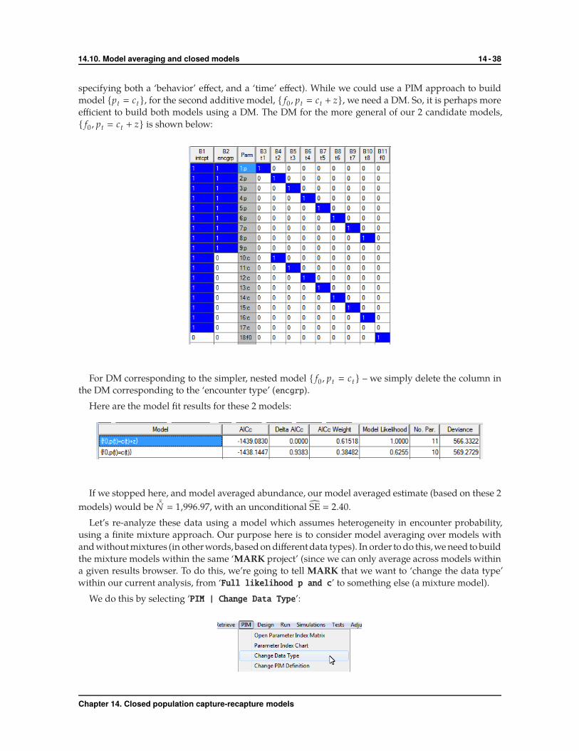
14.10. Model averaging and closed models 14 - 38
specifying both a ‘behavior’ effect, and a ‘time’ effect). While we could use a PIM approach to build
model {pt � ct }, for the second additive model, { f0 , pt � ct + z}, we need a DM. So, it is perhaps more
efficient to build both models using a DM. The DM for the more general of our 2 candidate models,
{ f0 , pt � ct + z} is shown below:
For DM corresponding to the simpler, nested model { f0 , pt � ct } – we simply delete the column in
the DM corresponding to the ‘encounter type’ (encgrp).
Here are the model fit results for these 2 models:
If we stopped here, and model averaged abundance, our model averaged estimate (based on these 2
models) would be ¯N � 1,996.97, with an unconditional SE � 2.40.
Let’s re-analyze these data using a model which assumes heterogeneity in encounter probability,
using a finite mixture approach. Our purpose here is to consider model averaging over models with
and without mixtures (in otherwords,based on different data types). In order to do this,we need to build
the mixture models within the same ‘MARK project’ (since we can only average across models within
a given results browser. To do this, we’re going to tell MARK that we want to ‘change the data type’
within our current analysis, from ‘Full likelihood p and c’ to something else (a mixture model).
We do this by selecting ‘PIM | Change Data Type’:
Chapter 14. Closed population capture-recapture models

14.10. Model averaging and closed models 14 - 39
MARK will then present all the available data types which are consistent with your data, letting you
select the one you want to change to. Here, we select ‘Full likelihood heterogeneity pi, p and c’:
Once we’ve selected the new data type, MARK will ask you how many finite mixtures you want to
model. We’ll accept the default of 2 mixture groups. MARK will then drop you back into the browser –
the only indication that the underlying data type has been changed is that the title of the results browser
now says ‘Full likelihood heterogeneity pi, p, and c’.
The PIM chart (below) is another indication that the underlying data type has changed.
We see (above) that the default model now has the mixture parameter, π, with full time dependence
for both encounter parameters, p and c.
Here, we’ll fit model { f0 , π, pA,t � cA,t + zA , pB ,t � cB ,t + zB} to the data (i.e., {pt � ct + z}, but
separately within each of the 2 mixture groups). The DM for this model is shown at the top of the next
page.
Chapter 14. Closed population capture-recapture models

14.10. Model averaging and closed models 14 - 40
If we fit this model to the data, and add the results to the browser (below), we see that this new
‘heterogeneity model’ gets roughly 84% of the support in the data among our 3 candidate models:
But, our interest here concerns model averaging. If at this point, having just fit the heterogeneity
model, { f0 , π, pA,t � cA,t + zA , pB ,t � cB ,t + zB}, we run through the (by now) familiar mechanics of
model averaging for N , we would see only one model reported in the model averaging output (shown
at the top of the next page).
Chapter 14. Closed population capture-recapture models
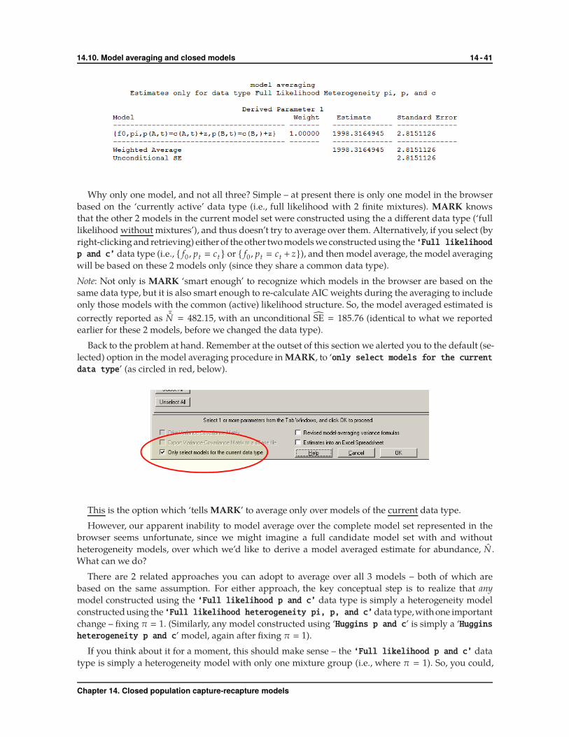
14.10. Model averaging and closed models 14 - 41
Why only one model, and not all three? Simple – at present there is only one model in the browser
based on the ‘currently active’ data type (i.e., full likelihood with 2 finite mixtures). MARK knows
that the other 2 models in the current model set were constructed using the a different data type (‘full
likelihood without mixtures’), and thus doesn’t try to average over them. Alternatively, if you select (by
right-clicking and retrieving) eitherof the other two models we constructed using the ‘Full likelihood
p and c’ data type (i.e., { f0 , pt � ct } or { f0 , pt � ct + z}), and then model average, the model averaging
will be based on these 2 models only (since they share a common data type).
Note: Not only is MARK ‘smart enough’ to recognize which models in the browser are based on the
same data type, but it is also smart enough to re-calculate AIC weights during the averaging to include
only those models with the common (active) likelihood structure. So, the model averaged estimated is
correctly reported as ¯N � 482.15, with an unconditional SE � 185.76 (identical to what we reported
earlier for these 2 models, before we changed the data type).
Back to the problem at hand. Remember at the outset of this section we alerted you to the default (se-
lected) option in the model averaging procedure in MARK, to ‘only select models for the current
data type’ (as circled in red, below).
This is the option which ‘tells MARK’ to average only over models of the current data type.
However, our apparent inability to model average over the complete model set represented in the
browser seems unfortunate, since we might imagine a full candidate model set with and without
heterogeneity models, over which we’d like to derive a model averaged estimate for abundance, N .
What can we do?
There are 2 related approaches you can adopt to average over all 3 models – both of which are
based on the same assumption. For either approach, the key conceptual step is to realize that any
model constructed using the ‘Full likelihood p and c’ data type is simply a heterogeneity model
constructedusing the ‘Full likelihood heterogeneity pi, p, and c’data type,withone important
change – fixing π � 1. (Similarly, any model constructed using ‘Huggins p and c’ is simply a ‘Huggins
heterogeneity p and c’ model, again after fixing π � 1).
If you think about it for a moment, this should make sense – the ‘Full likelihood p and c’ data
type is simply a heterogeneity model with only one mixture group (i.e., where π � 1). So, you could,
Chapter 14. Closed population capture-recapture models

14.10. Model averaging and closed models 14 - 42
if you wanted to, force the ‘Full likelihood heterogeneity pi, p, and c’ data type to fit models
for the ‘Full likelihood p and c’ data type, simply by fixing the mixture parameter π to 1. We’ll
consider this approach in a moment.
The quickest approach to handling model averaging in this case is to ‘tell MARK’ to ignore the fact
that, structurally, there are two different data types in the browser. We can do this here because, in fact,
the ‘Full likelihood p and c’ data type is simply a full likelihood heterogeneity model where π is
fixed to 1. In other words, although the models represent two different data types, they have the same
underlying likelihood structure. In fact, one data type is equivalent to the other, subject to a particular
constraint on one of the parameters (i.e., fixing π � 1).
So, we run through the mechanics of model averaging, except that this time, we ‘turn off’ the option
to restrict averaging to only models of the current data type, by unchecking the appropriate check-box,
as shown below:
Now,when you uncheck this option,MARK will respond with the following rather ominous warning
message when you try to average over models:
Here, ‘use at your own risk’ means ‘make sure you know what you’re doing...’. In this instance, we’ll
assume our underlying logic is correct, and so we can proceed with the final steps of model averaging
abundance N .
Here are the estimates:
We see that now, MARK averages over all 3 of the models in the browser – the model averaged
estimate for abundance is ¯N � 1,998.10, with an unconditional SE � 2.80
Chapter 14. Closed population capture-recapture models

14.10. Model averaging and closed models 14 - 43
However, are these estimates correct? Did we in fact ‘know what we were doing’ when we overrode
MARK’s warning about averaging over data types? Was our underlying logic that in fact these models
have the same underlying likelihood structure correct? We can prove to ourselves that ‘we got things
right’ (and confirm that MARK has given us the correct estimates using the preceding approach) by
(i) reconstructing the model set using the same data type for all three models, and (ii) manually fixing
π � 1 for two of them. While this is easy enough in principle, in practice this approach will require some
thought, since you’re going to need to think through carefully which columns in the ‘Full likelihood
heterogeneity pi, p, and c’ data type DM you need to keep, or modify, when you are reducing the
number of heterogeneity groups to 1 (i.e., single mixture group).
To start, have another look at the DM for model { f0 , π, pA,t � cA,t + zA , pB ,t � cB ,t + zB}, shown on
p. 31. Notice that there is a column for ‘hetgrp’, to account for the 2 mixture groups in this model. If
we want to force this model to be equivalent to a model without heterogeneity, without switching the
underlying data type, we need to do 2 things: (1) delete the ‘hetgrp’ column from the DM, and (2) fix
π � 1 before starting the numerical estimation run.
Go ahead and delete the ‘hetgrp’ column from the DM. What is the model represented by this DM?
If you look closely, and think about it a bit, you’ll realize that without the ‘hetgrp’ column, you’re left
with model {pt � ct + z}. Go ahead and run this model – call it ‘f0,pi=1,p(t)=c(t)+z’ (we’ll use ‘pi=1’
in the model name to indicate we built this model using only a single mixture group). Remember to fix
π � 1 before starting the numerical estimation.
When finished, add the results to the browser:
The deviances for model ‘f0,pi=1,p(t)=c(t)+z’ and model ‘f0,p(t)=c(t)+z’ are identical (meaning,
they are the same model!).
Next, how would we build model {pt � ct}, using the heterogeneity model approach? Simple – in
addition to deleting the ‘hetgrp’ column, we now also delete the ‘encgrp’ column (leaving only ’pi’,
’incpt’, the time columns (’t1’ → ’t9’), and N. Go ahead and delete the ‘encgrp’ column, fix π � 1, and
add the results to the browser (call this model ‘pi=1,p(t)=c(t)’).
Again, we see that fits for model ‘f0,pi=1,p(t)=c(t)’ and model ‘f0,p(t)=c(t)’ are identical
(meaning, once again, that they are the same model!).
OK, now for the big moment. We’ve proven to ourselves that we can build models for the ‘Full
likelihood p and c’data type using the‘Full likelihood heterogeneity pi, p, and c’data type,
simply by fixing π � 1, and making appropriate modifications to the DM (paying particular attention
Chapter 14. Closed population capture-recapture models

14.10.1. Estimating CI for model averaged abundance estimates 14 - 44
to terms involving the ‘heterogeneity group’ column). So, in fact, we could have built all 3 candidate
models ({pt � ct }, {pt � ct + z} and {π, pA,t � cA,t + zA , pB ,t � cB ,t + zB}), using the ‘Full likelihood
heterogeneity pi, p, and c’ data type – meaning, a single common data type. Meaning, we can
model average overall 3models without overriding the default option in MARK that prevents averaging
over models built using different data types.
Go ahead and delete models ‘p(t)=c(t)+z’ and ‘p(t)=c(t)’ from the browser, leaving only those
models built using the ‘Full likelihood heterogeneity pi, p, and c’ data type (i.e., all 3 models
in the browser are based on the same underlying data type).
Now, the big moment – go ahead and derivea model averaged estimate for ¯N , based on these 3 models
– without unchecking the ‘Only select models for the current data type’ (since these models are
all of the same data type):
Using this approach, the model averaged estimate for abundance is ¯N � 1,998.10, with an uncondi-
tional SE � 2.80, which are identical to the estimates we derived earlier.
Given the preceding, there is a fair argument to be made that you should only use the ‘heterogeneity
pi, p, and c’ data types (for either the full or conditional likelihoods), since it allows you to model
average over all the candidate models. However, keeping track of ‘encounter groups’ and ‘heterogeneity
groups’ does require more work to get things right. As long as you understandwhatyou’re doing,simply
forcing MARK to average over both data types is decidedly quicker. But, remember – you can only
average over models with a common likelihood structure: full likelihood (with and without mixtures),
or Huggins conditional likelihood (with and without mixtures).
14.10.1. Estimating CI for model averaged abundance estimates
The usual (simplest) approach to estimating the confidence interval for a given parameter makes use of
asymptotic variances, covariances – typically, these can be generated from the information matrix for
models with maximum likelihood estimates (this is discussed elsewhere).
However, there is a basic problem with applying this ‘classical’ approach to estimates of abundance
– specifically, the classical approach requires asymptotic normality of point estimates N , and this
assumption is frequently not met for any number of reasons.
Chapter 14. Closed population capture-recapture models
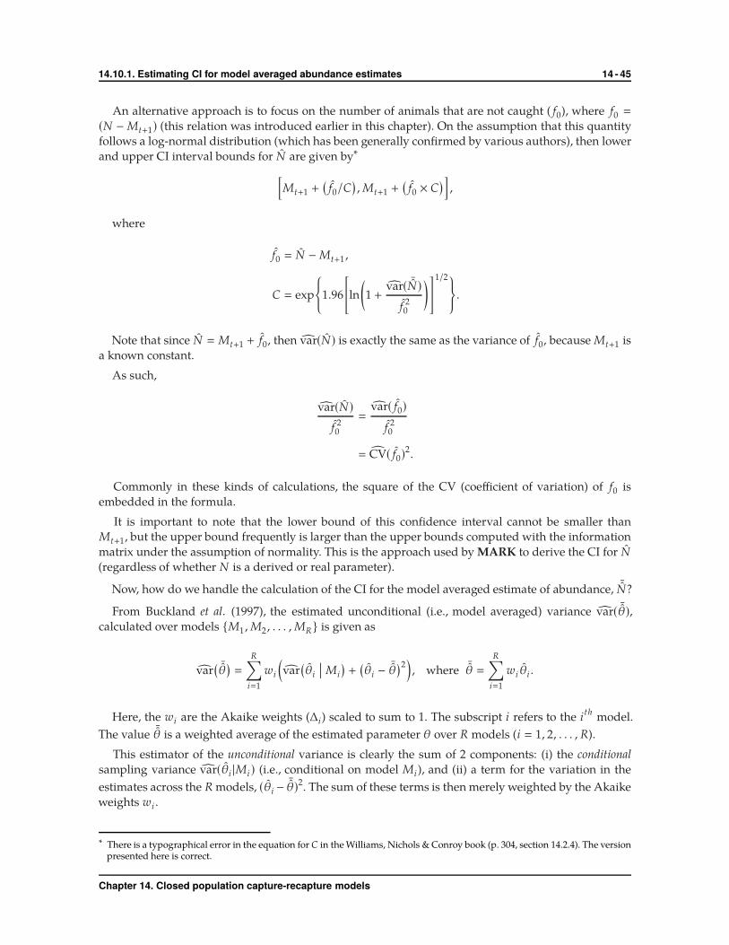
14.10.1. Estimating CI for model averaged abundance estimates 14 - 45
An alternative approach is to focus on the number of animals that are not caught ( f0), where f0 �
(N − Mt+1) (this relation was introduced earlier in this chapter). On the assumption that this quantity
follows a log-normal distribution (which has been generally confirmed by various authors), then lower
and upper CI interval bounds for N are given by∗
[Mt+1 +
(f0/C
),Mt+1 +
(f0 × C
) ],
where
f0 � N − Mt+1 ,
C � exp
{1.96
[ln
(1 +
var( ¯N)
f 20
)]1/2}.
Note that since N � Mt+1 + f0, then var(N) is exactly the same as the variance of f0, because Mt+1 is
a known constant.
As such,
var(N)
f 20
�
var( f0)
f 20
� CV( f0)2.
Commonly in these kinds of calculations, the square of the CV (coefficient of variation) of f0 is
embedded in the formula.
It is important to note that the lower bound of this confidence interval cannot be smaller than
Mt+1, but the upper bound frequently is larger than the upper bounds computed with the information
matrix under the assumption of normality. This is the approach used by MARK to derive the CI for N
(regardless of whether N is a derived or real parameter).
Now, how do we handle the calculation of the CI for the model averaged estimate of abundance, ¯N?
From Buckland et al. (1997), the estimated unconditional (i.e., model averaged) variance var( ¯θ),
calculated over models {M1 ,M2 , . . . ,MR} is given as
var( ¯θ
)�
R∑
i�1
wi
(var
(θi
�� Mi
)+
(θi −
¯θ)2
), where ¯θ �
R∑
i�1
wi θi .
Here, the wi are the Akaike weights (∆i) scaled to sum to 1. The subscript i refers to the ith model.
The value ¯θ is a weighted average of the estimated parameter θ over R models (i � 1, 2, . . . , R).
This estimator of the unconditional variance is clearly the sum of 2 components: (i) the conditional
sampling variance var(θi |Mi ) (i.e., conditional on model Mi), and (ii) a term for the variation in the
estimates across the R models, (θi −¯θ)2. The sum of these terms is then merely weighted by the Akaike
weights wi .
∗ There is a typographical error in the equation for C in the Williams, Nichols & Conroy book (p. 304, section 14.2.4). The versionpresented here is correct.
Chapter 14. Closed population capture-recapture models
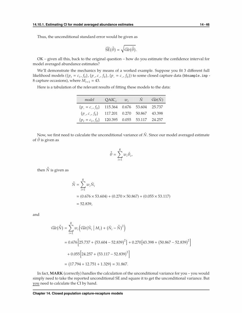
14.10.1. Estimating CI for model averaged abundance estimates 14 - 46
Thus, the unconditional standard error would be given as
SE( ¯θ
)�
√var
( ¯θ).
OK – given all this, back to the original question – how do you estimate the confidence interval for
model averaged abundance estimates?
We’ll demonstrate the mechanics by means of a worked example. Suppose you fit 3 different full
likelihood models ({pt � ct , f0}, {p· , c· , f0}, {p· � c· , f0}) to some closed capture data (bbsample.inp -
8 capture occasions), where Mt+1 � 43.
Here is a tabulation of the relevant results of fitting these models to the data:
model QAICc wi N var(N)
{p· � c· , f0} 115.364 0.676 53.604 25.737
{p· , c· , f0} 117.201 0.270 50.867 43.398
{pt � ct , f0} 120.395 0.055 53.117 24.257
Now, we first need to calculate the unconditional variance of N . Since our model averaged estimate
of θ is given as
¯θ �
R∑
i�1
wi θi ,
then ¯N is given as
¯N �
R∑
i�1
wi Ni
� (0.676 × 53.604) + (0.270 × 50.867) + (0.055 × 53.117)
� 52.839,
and
var( ¯N
)�
R∑
i�1
wi
(var
(Ni
�� Mi
)+
(Ni −
¯N)2
)
� 0.676[25.737 +
(53.604 − 52.839
)2]+ 0.270
[43.398 +
(50.867 − 52.839
)2]
+ 0.055[24.257 +
(53.117 − 52.839
)2]
�
(17.794 + 12.751 + 1.329
)� 31.867.
In fact, MARK (correctly) handles the calculation of the unconditional variance for you – you would
simply need to take the reported unconditional SE and square it to get the unconditional variance. But
you need to calculate the CI by hand.
Chapter 14. Closed population capture-recapture models

14.10.1. Estimating CI for model averaged abundance estimates 14 - 47
To do so, we first calculate
C � exp
{1.96
[ln
(1 +
var( ¯N
)
f 20
)]1/2}.
Since Mt+1 � 43 for this data set, and since ¯N � 52.839, then
¯f0 �
¯N − Mt+1
� (52.839 − 43)
� 9.839,
and thus
C � exp
{1.96
[ln
(1 +
var( ¯N
)
f 20
)]1/2}
� exp
{1.96
[ln
(1 +
31.867
(9.839)2
)]1/2}
� 2.845.
Last step. Now that we have a value for C, we can derive the 95% CI as
[43 +
(9.839/2.845
), 43 +
(9.839 × 2.845
)]� [46.458, 70.992].
OK, this seems like a lot of work,but in this particular example, it was necessary. If we had simply used
the ‘automatic’ model averaging in MARK, the CI reported by MARK for ¯N is [41.775, 63.905]. There
is clearly a fundamental problem with this CI, since the lower bound is less than Mt+1 (41.775 < 43).
Clearly, this makes no sense whatsoever. In contrast, the CI we derived ‘by hand’ does not bound Mt+1.
Not only was the reported lower-limit of the CI too low, but the upper limit was as well.
Now, in the preceding example, there was an obvious ‘problem’ with the simple model-averaged CI
for ¯N reported by MARK. However, even if the lower bound of the reported CI is ≥ Mt+1, don’t take
this as evidence that the reported CI is correct.
For example, consider fitting models { f0 , p(·) � c(·)} and { f0 , p(·), c(·)} to the ‘Carothers A’ data set
(found in the \examples subdirectory created when you installed MARK).
Here is a tabulation of the relevant results of fitting these models to the data:
model QAICc wi N var(N)
{ f0 , p(·) � c(·)} −99.7370 0.63460 368.128 212.944
{ f0 , p(·), c(·)} −98.6330 0.36540 392.480 1234.986
If we had used the model averaging option in MARK, the model averaged estimate is ¯N � 377.027,
and the reported 95% CI is [324.292, 429.761]. For this data set, Mt+1 � 283, so, in one sense at least,
the reported CI for the model average abundance estimate seems reasonable, since the lower limit of the
CI is greater than Mt+1 (i.e., 324.292 > 283). How does the reported CI compare with the one derived
using the calculations presented above?
Chapter 14. Closed population capture-recapture models
14.10.1. Estimating CI for model averaged abundance estimates 14 - 48
Again, we start by first deriving an estimate of the variance of the model averaged abundance:
var( ¯N
)�
R∑
i�1
wi
(var
(Ni
�� Mi
)+
(Ni −
¯N)2
)
� 0.63460(212.944 +
(368.128 − 377.027
)2)
+ 0.36540(1234.986+
(392.480 − 377.027
)2)
� 723.910.
Note that if we were to fit these models in MARK, the unconditional SE for the model averaged
abundance would be reported as 26.9045. If we square this value, we get (26.9045)2 � 723.901.
Again, the unconditional SE – and thus the variance – reported by MARK is correct (i.e., you do
not need to calculate the SE – or variance – by hand. We are simply demonstrating the underlying
calculations).
However, the CI as reported by MARK is not correct – this, you need to do by hand.
As in the first example, we first calculate
C � exp
{1.96
[ln
(1 +
var( ¯N
)
f 20
)]1/2}.
Since Mt+1 � 283 for this data set, and since ¯N � 377.027, then
f0 �¯N − Mt+1
� (377.027 − 283)
� 94.027.
Thus,
C � exp
{1.96
[ln
(1 +
723.910
(94.027)2
)]1/2}
� 1.733.
Final step. Now that we have a value for C, we can construct the 95% CI around the model averaged
estimate ¯N � 377.027 as
[283 +
(94.027/1.733
), 283 +
(94.027 × 1.744
)]�⇒
[337.26, 445.94
].
Recall that if we had used the model averaging option in MARK, the reported model averaged 95%
CI was [324.292, 429.758]. Again, these reported lower- and upper-limits of the CI are both different
than the ones we just calculated ‘by hand’.
The general recommendation, then, is to calculate the 95% CI for the model averaged abundance ‘by
hand’, using the procedure outlined above.
Chapter 14. Closed population capture-recapture models
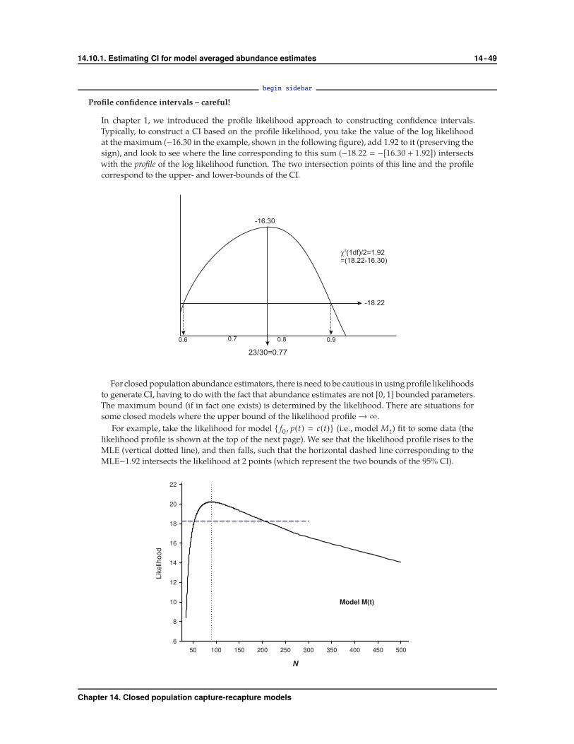
14.10.1. Estimating CI for model averaged abundance estimates 14 - 49
begin sidebar
Profile confidence intervals – careful!
In chapter 1, we introduced the profile likelihood approach to constructing confidence intervals.
Typically, to construct a CI based on the profile likelihood, you take the value of the log likelihood
at the maximum (−16.30 in the example, shown in the following figure), add 1.92 to it (preserving the
sign), and look to see where the line corresponding to this sum (−18.22 � −[16.30 + 1.92]) intersects
with the profile of the log likelihood function. The two intersection points of this line and the profile
correspond to the upper- and lower-bounds of the CI.
For closed population abundance estimators, there is need to be cautious in using profile likelihoods
to generate CI, having to do with the fact that abundance estimates are not [0, 1] bounded parameters.
The maximum bound (if in fact one exists) is determined by the likelihood. There are situations for
some closed models where the upper bound of the likelihood profile → ∞.
For example, take the likelihood for model { f0 , p(t) � c(t)} (i.e., model Mt ) fit to some data (the
likelihood profile is shown at the top of the next page). We see that the likelihood profile rises to the
MLE (vertical dotted line), and then falls, such that the horizontal dashed line corresponding to the
MLE−1.92 intersects the likelihood at 2 points (which represent the two bounds of the 95% CI).
N
50 100 150 200 250 300 350 400 450 500
Lik
elih
oo
d
6
8
10
12
14
16
18
20
22
Model M(t)
Chapter 14. Closed population capture-recapture models
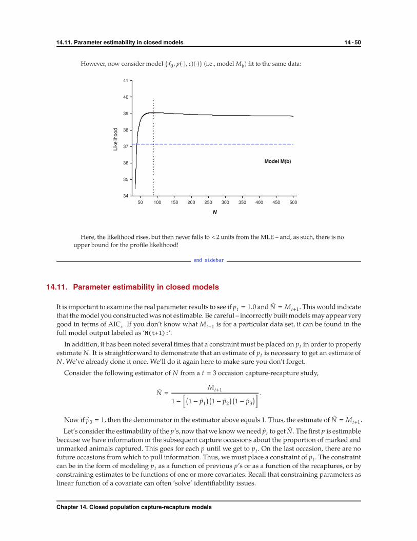
14.11. Parameter estimability in closed models 14 - 50
However, now consider model { f0 , p(·), c)(·)} (i.e., model Mb) fit to the same data:
N
50 100 150 200 250 300 350 400 450 500
Lik
elih
oo
d
34
35
36
37
38
39
40
41
Model M(b)
Here, the likelihood rises, but then never falls to <2 units from the MLE – and, as such, there is no
upper bound for the profile likelihood!
end sidebar
14.11. Parameter estimability in closed models
It is important to examine the real parameter results to see if pt � 1.0 and N � Mt+1. This would indicate
that the model you constructed was not estimable. Be careful – incorrectly built models may appear very
good in terms of AICc . If you don’t know what Mt+1 is for a particular data set, it can be found in the
full model output labeled as ‘M(t+1):’.
In addition, it has been noted several times that a constraint must be placed on pt in order to properly
estimate N . It is straightforward to demonstrate that an estimate of pt is necessary to get an estimate of
N . We’ve already done it once. We’ll do it again here to make sure you don’t forget.
Consider the following estimator of N from a t � 3 occasion capture-recapture study,
N �
Mt+1
1 −[(
1 − p1
) (1 − p2
) (1 − p3
) ] .
Now if p3 � 1, then the denominator in the estimator above equals 1. Thus, the estimate of N � Mt+1.
Let’s consider the estimability of the p’s, now that we know we need pt to get N . The first p is estimable
because we have information in the subsequent capture occasions about the proportion of marked and
unmarked animals captured. This goes for each p until we get to pt . On the last occasion, there are no
future occasions from which to pull information. Thus, we must place a constraint of pt . The constraint
can be in the form of modeling pt as a function of previous p’s or as a function of the recaptures, or by
constraining estimates to be functions of one or more covariates. Recall that constraining parameters as
linear function of a covariate can often ‘solve’ identifiability issues.
Chapter 14. Closed population capture-recapture models
14.12. Other applications 14 - 51
14.12. Other applications
Closed population capture-recapture models have been used for other applications beyond estimating
the number of individuals in a population. There is a natural extension to estimating the number of
species in an area. In this case,encounterhistories representdetections of species rather than individuals.
Heterogeneity in detection probability among species is virtually guaranteed.
Closed capture-recapture models and modifications thereof are widely used in human demography.
There they are typically referred to as multiple list sampling. Several lists containing people from a
population of interest, for example drug users in a city, act as sampling occasions. Individuals are
matched across lists to estimate abundance.
The closed population capture-recapture models underpin the secondary sampling periods in a
robust design (Kendall et al. 1997; see Chapter 15). It is therefore essential to understand the closed
captures models in order to fully understand the robust design
14.13. Summary
Despite a seemingly simple goal, estimating abundance can be quite difficult. The closed capture-
recapture models contain numerous, subtle complications. MARK offers a framework for a variety
of models addressing different assumptions, compares models and most importantly model averages
estimated abundance.
An additional advantage of MARK is the ability to combine data from multiple study sites. It is too
often argued in the ecological literature that capture-recapture is not useful because the sample size at
any one trapping grid is too small. Through the use of groups, MARK allows data from multiple grids
to be used to jointly estimate detection probability. While this may bias the estimate of N somewhat
for each individual grid, it remains a better solution than using minimum number known alive as an
index. Moreover, MARK handles all of the covariances among the N’s estimated from common data.
14.14. References
Boulanger, J., White, G. C., McLellan, B.N., Woods, J., Proctor, M., and Himmer, S. (2002) A meta-analysis
of grizzly bear DNA mark-recapture projects in British Columbia, Canada. Ursus, 13, 137-152.
Carothers, A. D. (1973) Capture-recapture methods applied to a population with known parameters.
Journal of Animal Ecology, 42, 125-146.
Dorazio, R. M., and Royle, J. A. (2003) Mixture models for estimating the size of a closed population
when capture rates vary among individuals. Biometrics, 59, 351-364.
Fletcher, D. (2012) Estimating overdispersion when fitting a generalized linear model to sparse data.
Biometrika, 99, 230-237.
Gimenez, O., and Choquet, R. (2010) Individual heterogeneity in studies on marked animals using
numerical integration: capture-recapture mixed models. Ecology, 91, 951-957.
Huggins, R. M. (1989) On the statistical analysis of capture experiments. Biometrika, 76, 133-140.
Kendall, W. L., Nichols, J. D., and Hines, J. E. (1997) Estimating temporary emigration using capture-
recapture data with Pollock’s robust design. Ecology, 78, 563-578.
Link, W. A. (2003) Non-identifiability of population size from capture-recapture data with heteroge-
neous detection probabilities. Biometrics, 59, 1125-1132.
Chapter 14. Closed population capture-recapture models

14.14. References 14 - 52
Link, W. A. (2004) Individual heterogeneity and identifiability in capture-recapture models. Animal
Biodiversity and Conservation, 27, 441-449.
Liu, Q., and Pierce, D. (1994) A note on Gauss-Hermite quadrature. Biometrika, 81, 624-629.
Lukacs, P. M., and Burnham, K. P. (2005) Estimating population size from DNA-based closed capture-
recapture data incorporating genotyping error. Journal of Wildlife Management, 69, 396-403.
McClintock, B. T., White, G. C., Burnham, K. P., and Pryde, M. A. (2009) A generalized mixed effects
model of abundance for mark-resight data when sampling is without replacement. Pages 271-289
in D. L. Thomson, E. G. Cooch, and M. J. Conroy, editors. Modeling Demographic Processes in Marked
Populations – Environmental and Ecological statistics 3. Springer, New York, New York, USA.
Norris, J. L., and Pollock, K. H. (1996) Nonparametric MLE under two closed capture-recapture models
with heterogeneity. Biometrics, 52, 639-649.
Otis, D. L., Burnham, K. P., White, G. C., and Anderson, D. R. (1978) Statistical inference from capture
data on closed animal populations. Wildlife Monographs, 62.
Pledger, S. (2000) Unified maximum likelihood estimates for closed capture-recapture models using
mixtures. Biometrics, 56, 434-442.
Pledger, S. (2005) The performance of mixture models in heterogeneous closed population capture-
recapture. Biometrics, 61, 868-873
Pledger,S., and Phillpot,P. (2008) Using mixtures to model heterogeneity in ecological capture-recapture
studies. Biometrical Journal, 50, 1022-1034
Powell, L. A., and Gale, G. A. (2015) Estimation of Parameters for Animal Populations. Caught Napping
Publications, Lincoln, NE. 256 pp.
Seber, G. A. F., and Whale, J. F. (1970) The removal method for two and three samples. Biometrics, 26,
393-400.
Stanley, T. R., and Burnham, K. P.. (1999) A closure test for time-specific capture-recapture data. Envi-
ronmental and Ecological Statistics, 6, 197-209.
Stanley, T. R., and K. P. Burnham. 1998. Information-theoretic model selection and model averaging for
closed-population capture-recapture studies. Biometrical Journal, 40, 475-494.
White, G. C., Anderson, D. R., Burnham, K. P., and Otis, D. L. (1982) Capture-recapture and removal
methods for sampling closed populations. Los Alamos National Laboratory Publication LA-8787-
NERP. Los Alamos, NM.
White, G. C., and Cooch, E. G. (2017) Population abundance estimation with heterogeneous encounter
probabilities using numerical integration. Journal of Wildlife Management, 81, 322-336.
Chapter 14. Closed population capture-recapture models

Addendum – heterogeneity modeling 14 - 53
Addendum – heterogeneity modeling for other data types
Heterogeneity is a common, verging on ubiquitous issue, regrdless of the data type, or type of analysis
you’re working with. When individual animals do not behave identically with the same exact detection
or survival probability, extra-binomial variation or overdispersion occurs. Each animal has its own
parameter value, leading to parameter heterogeneity. The extra-binomial variation causes standard
errors of parameter estimates to be too small, i.e., too precise, because this extra variation is not
recognized in the model.
Two approaches are available in MARK for some data types to model individual heterogeneity. While
there are no perfect solutions to handling heterogeneity in general, use of discrete- and continuous-
mixture models has proven to be a robustapproach in many cases. In bothcases,more than≥ 5 occasions
are required to be able to detect and account for individual heterogeneity in any reasonable. That is, the
animal (or plot for occupancy) must be observed multiple times to be able to detect and estimate the
heterogeneity.
Finite-mixture models
Pledger (2000) and Pledger et al. (2003) proposed using finite-mixture models to model heterogeneity.
This approach has been implemented for the ‘encounter probability’ parameter in MARK for a variety
of data types, and for both ‘encounter’ and ‘survival’, or ‘survival’ only for others:
data type parameter(s) with mixture option chapter(s)
closed captures p , c Chapter 14
robust design p , c Chapter 15
Cormack-Jolly-Seber ϕ, p Chapter 3 → 8
Pradel p Chapter 13
robust-design Pradel p –
Link-Barker p Chapter 12
Seber dead recovery S Chapter 8
occupancy (single season) p Chapter 21
occupancy (multi-season) p Chapter 21
Continuous-mixture models
The second method of modeling individual heterogeneity is to add a normally-distributed random
error with standard deviation σ to the logit value of the parameter, then numerically integrate out this
random error. The first data type in MARK that did this was the logit-normal mark-resight estimator
(McClintock & White 2009, McClintock et al. 2009, Chapter 18). Gimenez & Choquet (2010) proposed
the same approach for Cormack-Jolly-Seber models. Because of the relative simplicity of the approach,
and seemingly more biologically realistic, the approach has been incorporated with a number of MARK
data types.
Because the random effect is numerically integrated out of the model using Gaussian-Hermite
quadrature (this chapter,Gimenez & Choquet 2010,White & Cooch 2017), the computer time to run these
Chapter 14. Closed population capture-recapture models

Addendum – heterogeneity modeling 14 - 54
models is significantly greater than the corresponding model without the random effect. The default
in MARK is to integrate over 101 nodes, so roughly 101 times the computing time is needed compared
to the data type that does not include the random effect. Further, for data types that have multiple
random effects, such as the Cormack-Jolly-Seber or Link-Barker, the integration loops are nested. So for
the Cormack-Jolly-Seber data type with random effects being estimated for both ϕ and p, the CPU time
will be approximately (101 × 101) � 10,201 times longer than a normal Cormack-Jolly-Seber model. Be
advised!
The number of nodes for Gaussian-Hermite quadrature canbe set in the ‘File | Preferences’ dialog
window. The minimum value allowed is 15, and the max 505. For 505 nodes, the weights are zero for
at least 15 nodes in each tail, so more nodes doesn’t actually improve precision in the tails. The default
(101) tends to work very well for most purposes.
A nice feature of this approach is that the estimate of the σ parameter modeling the individual
heterogeneity is available. Thus, you can get some idea of how much individual heterogeneity is
provided around the mean value on the logit scale. Further, the σ parameter can be set to zero to
evaluate the impact of individual heterogeneity. In all cases, fixing the σ parameter to zero will give
exactly the same likelihood value as the model not including the random effect(s).
Data types in MARK where the individual random effects methodology has been implemented are
shown in the following:
data type parameter(s) with mixture option chapter(s)
mark-resight logit p Chapter 18
closed abundance, Huggins p , c Chapter 15
robust design, Huggins ϕ, p Chapter 3 → 8
Cormack-Jolly-Seber ϕ, p Chapter 3 → 8
robust-design Pradel p –
Link-Barker ϕ, p , f Chapter 12
Burnham live-dead S, F, p , r∗ Chapter 10
Seber dead recovery S, r∗ Chapter 9
occupancy p Chapter 21
known-fate S† Chapter 16
(∗) Parameters marked with a (∗) can have a random effect specified mainly for simulationpurposes. Because these parameters are only observed once in the probability of an encounterhistory, the random effect σ is not identifiable.
(†) S in the ‘known fate’ data type can be modeled with the saturated model in MARK. That is,you can create the saturated model and hence not be able to estimate the σS parameter becauseyou have made it not identifiable.
Chapter 14. Closed population capture-recapture models