Closed Loop Speed Control of a BLDC Motor Drive Using ... - 6/O04110693104.pdf · Closed Loop Speed Control of a BLDC Motor Drive Using Adaptive Fuzzy Tuned PI Controller Sri

Sri Latha Eti Int. Journal of Engineering Research and Applications www.ijera.com

ISSN : 2248-9622, Vol. 4, Issue 11(Version - 6), November 2014, pp.93-104

www.ijera.com 93 | P a g e

Closed Loop Speed Control of a BLDC Motor Drive Using

Adaptive Fuzzy Tuned PI Controller

Sri Latha Eti1 , Dr. N. Prema Kumar

2

1PG Scholar, Dept. of Electrical Engineering, A.U College of Engineering (A), Andhra University,

Visakhapatnam, A.P, India 2

Associate Professor, Dept. of Electrical Engineering, A.U College of Engineering (A), Andhra University,

Visakhapatnam, A.P, India

ABSTRACT Brushless DC Motors are widely used for many industrial applications because of their high efficiency, high

torque and low volume. This paper proposed an improved Adaptive Fuzzy PI controller to control the speed of

BLDC motor. This paper provides an overview of different tuning methods of PID Controller applied to control

the speed of the transfer function model of the BLDC motor drive and then to the mathematical model of the

BLDC motor drive. It is difficult to tune the parameters and get satisfied control characteristics by using normal

conventional PI controller. The experimental results verify that Adaptive Fuzzy PI controller has better control

performance than the conventional PI controller. The modeling, control and simulation of the BLDC motor have

been done using the MATLAB/SIMULINK software. Also, the dynamic characteristics of the BLDC motor (i.e.

speed and torque) as well as currents and voltages of the inverter components are observed by using the

developed model.

Keywords - BLDC motor, Motor drive, Conventional P, PI, PID Controllers, Different PID Tuning methods,

Adaptive fuzzy PI Controller

I. INTRODUCTION Permanent magnet brushless DC motors

(PMBLDC) find wide applications in industries due to

their high power density and ease of control. These

motors are generally controlled using a three phase

power semiconductor bridge. For starting and the

providing proper commutation sequence to turn on the

power devices in the inverter bridge the rotor position

sensors are required. Based on the rotor position, the

power devices are commutated sequentially every 60

degrees. To achieve desired level of performance the

motor requires suitable speed controllers. In case of

permanent magnet motors, usually speed control is

achieved by using proportional-integral (PI)

controller. Although conventional PI controllers are

widely used in the industry due to their simple control

structure and ease of implementation, these controllers

pose difficulties where there are some control

complexity such as nonlinearity, load disturbances and

parametric variations. Moreover PI controllers require

precise linear mathematical models. Fuzzy Logic

Controller (FLC) for speed control of a BLDC leads to

an improved dynamic behavior of the motor drive

system and immune to load perturbations and

parameter variations.

II. BLDC MOTOR MODELLING 2.1Simulation of BLDC motor

Brushless Direct Current (BLDC) motors are one of

the motor types rapidly gaining popularity. BLDC

motors are used in industries such as Appliances,

Automotive, Aerospace, Consumer, Medical,

Industrial Automation Equipment and

Instrumentation. As the name implies, BLDC motors

do not use brushes for commutation; instead, they are

electronically commutated. BLDC motors have many

advantages over brushed DC motors and induction

motors as in [1]. A few of these are better speed vs

torque characteristics, high dynamic response, high

efficiency, long operating life and noiseless

operation.

In addition, the ratio of torque delivered to the

size of the motor is higher, making it useful in

applications where space and weight are critical

factors. The BLDC motor is supplied from battery

through the inverter. The dynamic model of this

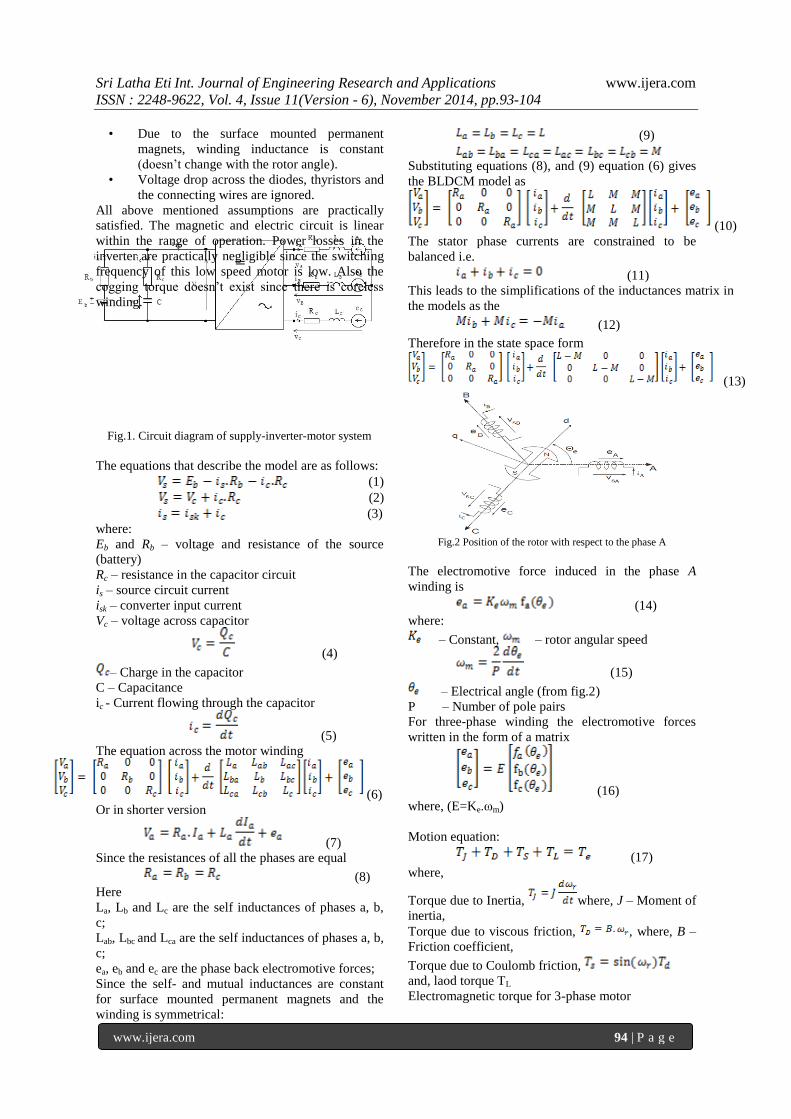
system is shown in Fig.1. It is derived under the

following assumptions[2]:

• All the elements of the motor are linear and

core losses are neglected.

• Induced currents in the rotor due to stator

harmonic fields are neglected.

• The electromotive force ea varies sinusoidal

with the rotational electric angle θe.

• The cogging torque of the motor is negligible.

RESEARCH ARTICLE OPEN ACCESS




• Due to the surface mounted permanent

magnets, winding inductance is constant

(doesn’t change with the rotor angle).

• Voltage drop across the diodes, thyristors and

the connecting wires are ignored.

All above mentioned assumptions are practically

satisfied. The magnetic and electric circuit is linear

within the range of operation. Power losses in the

inverter are practically negligible since the switching

frequency of this low speed motor is low. Also the

cogging torque doesn’t exist since there is coreless

winding.

Fig.1. Circuit diagram of supply-inverter-motor system

The equations that describe the model are as follows:

(1)

(2)

(3)

where:

Eb and Rb – voltage and resistance of the source

(battery)

Rc – resistance in the capacitor circuit

is – source circuit current

isk – converter input current

Vc – voltage across capacitor

(4)

– Charge in the capacitor

C – Capacitance

ic - Current flowing through the capacitor

(5)

The equation across the motor winding

(6)

Or in shorter version

(7)

Since the resistances of all the phases are equal

(8)

Here

La, Lb and Lc are the self inductances of phases a, b,

c;

Lab, Lbc and Lca are the self inductances of phases a, b,

c;

ea, eb and ec are the phase back electromotive forces;

Since the self- and mutual inductances are constant

for surface mounted permanent magnets and the

winding is symmetrical:

(9)

Substituting equations (8), and (9) equation (6) gives

the BLDCM model as

(10)

The stator phase currents are constrained to be

balanced i.e.

(11)

This leads to the simplifications of the inductances matrix in

the models as the

(12)

Therefore in the state space form

(13)

Fig.2 Position of the rotor with respect to the phase A

The electromotive force induced in the phase A

winding is

(14)

where:

– Constant, – rotor angular speed

(15)

– Electrical angle (from fig.2)

P – Number of pole pairs

For three-phase winding the electromotive forces

written in the form of a matrix

(16)

where, (E=Ke.ωm)

Motion equation:

(17)

where,

Torque due to Inertia, where, J – Moment of

inertia,

Torque due to viscous friction, , where, B –

Friction coefficient,

Torque due to Coulomb friction,

and, laod torque TL

Electromagnetic torque for 3-phase motor




(18)

(19)

2.2 Modelling of Trapezoidal Back emf equations

The trapezoidal back emf waveforms are

modeled as a function of rotor position so that the

rotor position can be actively calculated according to

the operation speed[3]. The back emfs are expressed

as a function of rotor position ( ), which can be

written as:

(20)

where,

(21)

The trapezoidal back emf waveforms of a BLDC

motor are realized using trapezoidal shape function of

rotor position with limit values between +1 and -1

using Embedded matlab function.

2.3 Three phase Voltage source Inverter

Fig.3 Configuration of BLDC motor and Three Phase VSI system

Three phase bridge inverters are widely used for ac

motor drives and general purpose ac supplies. The

input dc supply is usually obtained from a battery or

from a single phase or three phase utility power

supply through diode bridge rectifier and LC or C

filter as shown in Fig.3. The capacitor tends to make

the input dc voltage constant. This also suppresses the

harmonics fed back to the dc source.

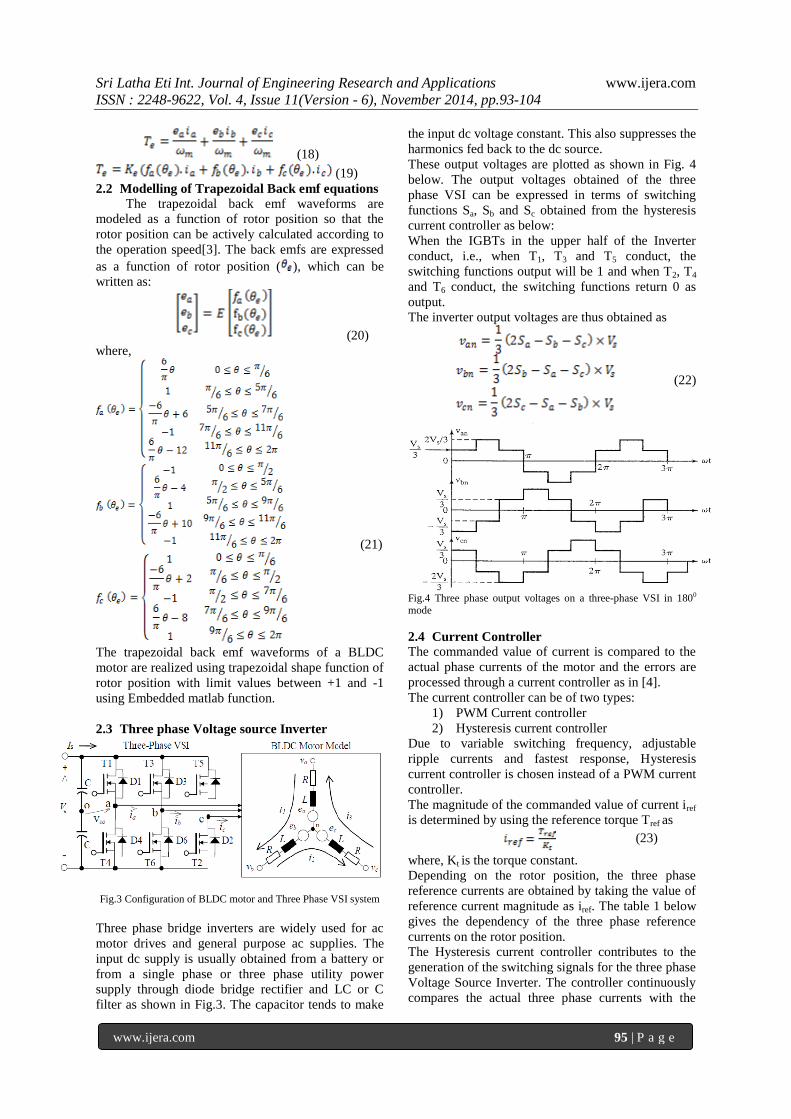
These output voltages are plotted as shown in Fig. 4

below. The output voltages obtained of the three

phase VSI can be expressed in terms of switching

functions Sa, Sb and Sc obtained from the hysteresis

current controller as below:

When the IGBTs in the upper half of the Inverter

conduct, i.e., when T1, T3 and T5 conduct, the

switching functions output will be 1 and when T2, T4

and T6 conduct, the switching functions return 0 as

output.

The inverter output voltages are thus obtained as

(22)

Fig.4 Three phase output voltages on a three-phase VSI in 1800 mode

2.4 Current Controller

The commanded value of current is compared to the

actual phase currents of the motor and the errors are

processed through a current controller as in [4].

The current controller can be of two types:

1) PWM Current controller

2) Hysteresis current controller

Due to variable switching frequency, adjustable

ripple currents and fastest response, Hysteresis

current controller is chosen instead of a PWM current

controller.

The magnitude of the commanded value of current iref

is determined by using the reference torque Tref as

(23)

where, Kt is the torque constant.

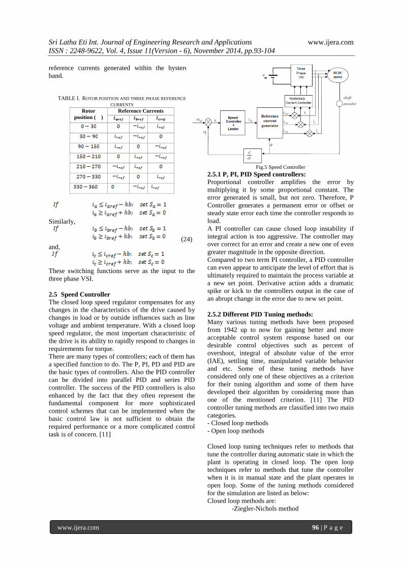
Depending on the rotor position, the three phase

reference currents are obtained by taking the value of

reference current magnitude as iref. The table 1 below

gives the dependency of the three phase reference

currents on the rotor position.

The Hysteresis current controller contributes to the

generation of the switching signals for the three phase

Voltage Source Inverter. The controller continuously

compares the actual three phase currents with the




reference currents generated within the hysteresis

band.

TABLE I. ROTOR POSITION AND THREE PHASE REFERENCE

CURRENTS

Rotor

position ( )

Reference Currents

Similarly,

(24)

and,

These switching functions serve as the input to the

three phase VSI.

2.5 Speed Controller

The closed loop speed regulator compensates for any

changes in the characteristics of the drive caused by

changes in load or by outside influences such as line

voltage and ambient temperature. With a closed loop

speed regulator, the most important characteristic of

the drive is its ability to rapidly respond to changes in

requirements for torque.

There are many types of controllers; each of them has

a specified function to do. The P, PI, PD and PID are

the basic types of controllers. Also the PID controller

can be divided into parallel PID and series PID

controller. The success of the PID controllers is also

enhanced by the fact that they often represent the

fundamental component for more sophisticated

control schemes that can be implemented when the

basic control law is not sufficient to obtain the

required performance or a more complicated control

task is of concern. [11]

Fig.5 Speed Controller

2.5.1 P, PI, PID Speed controllers: Proportional controller amplifies the error by

multiplying it by some proportional constant. The

error generated is small, but not zero. Therefore, P

Controller generates a permanent error or offset or

steady state error each time the controller responds to

load.

A PI controller can cause closed loop instability if

integral action is too aggressive. The controller may

over correct for an error and create a new one of even

greater magnitude in the opposite direction.

Compared to two term PI controller, a PID controller

can even appear to anticipate the level of effort that is

ultimately required to maintain the process variable at

a new set point. Derivative action adds a dramatic

spike or kick to the controllers output in the case of

an abrupt change in the error due to new set point.

2.5.2 Different PID Tuning methods:

Many various tuning methods have been proposed

from 1942 up to now for gaining better and more

acceptable control system response based on our

desirable control objectives such as percent of

overshoot, integral of absolute value of the error

(IAE), settling time, manipulated variable behavior

and etc. Some of these tuning methods have

considered only one of these objectives as a criterion

for their tuning algorithm and some of them have

developed their algorithm by considering more than

one of the mentioned criterion. [11] The PID

controller tuning methods are classified into two main

categories.

- Closed loop methods

- Open loop methods

Closed loop tuning techniques refer to methods that

tune the controller during automatic state in which the

plant is operating in closed loop. The open loop

techniques refer to methods that tune the controller

when it is in manual state and the plant operates in

open loop. Some of the tuning methods considered

for the simulation are listed as below:

Closed loop methods are:

-Ziegler-Nichols method




-Tyreus-Luyben method

Open loop methods are:

-Open loop Ziegler-Nichols method

-C-H-R method

-Cohen and Coon method

Let the transfer function of the PID controller be

(25)

where, kc- Proportional gain

τi- Integral time

τd- Derivative time

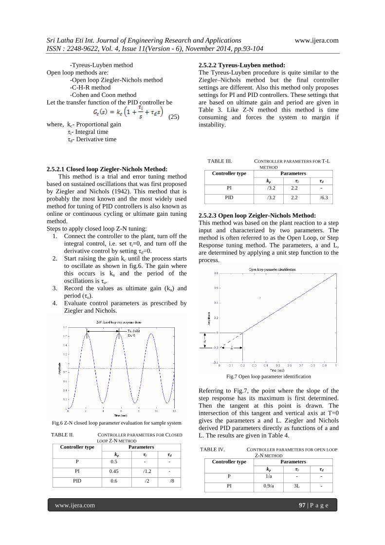
2.5.2.1 Closed loop Ziegler-Nichols Method:

This method is a trial and error tuning method

based on sustained oscillations that was first proposed

by Ziegler and Nichols (1942). This method that is

probably the most known and the most widely used

method for tuning of PID controllers is also known as

online or continuous cycling or ultimate gain tuning

method.

Steps to apply closed loop Z-N tuning:

1. Connect the controller to the plant, turn off the

integral control, i.e. set τi=0, and turn off the

derivative control by setting τd=0.

2. Start raising the gain kc until the process starts

to oscillate as shown in fig.6. The gain where

this occurs is ku and the period of the

oscillations is τu.

3. Record the values as ultimate gain (ku) and

period (τu).

4. Evaluate control parameters as prescribed by

Ziegler and Nichols.

Fig.6 Z-N closed loop parameter evaluation for sample system

TABLE II. CONTROLLER PARAMETERS FOR CLOSED

LOOP Z-N METHOD

Controller type Parameters

kp τi τd

P 0.5 - -

PI 0.45 /1.2 -

PID 0.6 /2 /8

2.5.2.2 Tyreus-Luyben method:

The Tyreus-Luyben procedure is quite similar to the

Ziegler–Nichols method but the final controller

settings are different. Also this method only proposes

settings for PI and PID controllers. These settings that

are based on ultimate gain and period are given in

Table 3. Like Z-N method this method is time

consuming and forces the system to margin if

instability.

TABLE III. CONTROLLER PARAMETERS FOR T-L

METHOD


kp τi τd

PI /3.2 2.2 -

PID /3.2 2.2 /6.3

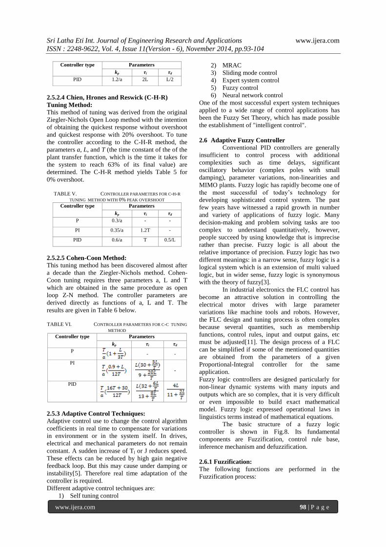
2.5.2.3 Open loop Zeigler-Nichols Method:

This method was based on the plant reaction to a step

input and characterized by two parameters. The

method is often referred to as the Open Loop, or Step

Response tuning method. The parameters, a and L,

are determined by applying a unit step function to the

process.

Fig.7 Open loop parameter identification

Referring to Fig.7, the point where the slope of the

step response has its maximum is first determined.

Then the tangent at this point is drawn. The

intersection of this tangent and vertical axis at T=0

gives the parameters a and L. Ziegler and Nichols

derived PID parameters directly as functions of a and

L. The results are given in Table 4.

TABLE IV. CONTROLLER PARAMETERS FOR OPEN LOOP

Z-N METHOD


kp τi τd

P 1/a - -

PI 0.9/a 3L -





kp τi τd

PID 1.2/a 2L L/2

2.5.2.4 Chien, Hrones and Reswick (C-H-R)

Tuning Method:

This method of tuning was derived from the original

Ziegler-Nichols Open Loop method with the intention

of obtaining the quickest response without overshoot

and quickest response with 20% overshoot. To tune

the controller according to the C-H-R method, the

parameters a, L, and T (the time constant of the of the

plant transfer function, which is the time it takes for

the system to reach 63% of its final value) are

determined. The C-H-R method yields Table 5 for

0% overshoot.

TABLE V. CONTROLLER PARAMETERS FOR C-H-R

TUNING METHOD WITH 0% PEAK OVERSHOOT


kp τi τd

P 0.3/a - -

PI 0.35/a 1.2T -

PID 0.6/a T 0.5/L

2.5.2.5 Cohen-Coon Method:

This tuning method has been discovered almost after

a decade than the Ziegler-Nichols method. Cohen-

Coon tuning requires three parameters a, L and T

which are obtained in the same procedure as open

loop Z-N method. The controller parameters are

derived directly as functions of a, L and T. The

results are given in Table 6 below.

TABLE VI. CONTROLLER PARAMETERS FOR C-C TUNING

METHOD


kp τi τd

P

- -

PI

-

PID

2.5.3 Adaptive Control Techniques:

Adaptive control use to change the control algorithm

coefficients in real time to compensate for variations

in environment or in the system itself. In drives,

electrical and mechanical parameters do not remain

constant. A sudden increase of Tl or J reduces speed.

These effects can be reduced by high gain negative

feedback loop. But this may cause under damping or

instability[5]. Therefore real time adaptation of the

controller is required.

Different adaptive control techniques are:

1) Self tuning control

2) MRAC

3) Sliding mode control

4) Expert system control

5) Fuzzy control

6) Neural network control

One of the most successful expert system techniques

applied to a wide range of control applications has

been the Fuzzy Set Theory, which has made possible

the establishment of "intelligent control".

2.6 Adaptive Fuzzy Controller

Conventional PID controllers are generally

insufficient to control process with additional

complexities such as time delays, significant

oscillatory behavior (complex poles with small

damping), parameter variations, non-linearities and

MIMO plants. Fuzzy logic has rapidly become one of

the most successful of today’s technology for

developing sophisticated control system. The past

few years have witnessed a rapid growth in number

and variety of applications of fuzzy logic. Many

decision-making and problem solving tasks are too

complex to understand quantitatively, however,

people succeed by using knowledge that is imprecise

rather than precise. Fuzzy logic is all about the

relative importance of precision. Fuzzy logic has two

different meanings: in a narrow sense, fuzzy logic is a

logical system which is an extension of multi valued

logic, but in wider sense, fuzzy logic is synonymous

with the theory of fuzzy[3].

In industrial electronics the FLC control has

become an attractive solution in controlling the

electrical motor drives with large parameter

variations like machine tools and robots. However,

the FLC design and tuning process is often complex

because several quantities, such as membership

functions, control rules, input and output gains, etc

must be adjusted[11]. The design process of a FLC

can be simplified if some of the mentioned quantities

are obtained from the parameters of a given

Proportional-Integral controller for the same

application.

Fuzzy logic controllers are designed particularly for

non-linear dynamic systems with many inputs and

outputs which are so complex, that it is very difficult

or even impossible to build exact mathematical

model. Fuzzy logic expressed operational laws in

linguistics terms instead of mathematical equations.

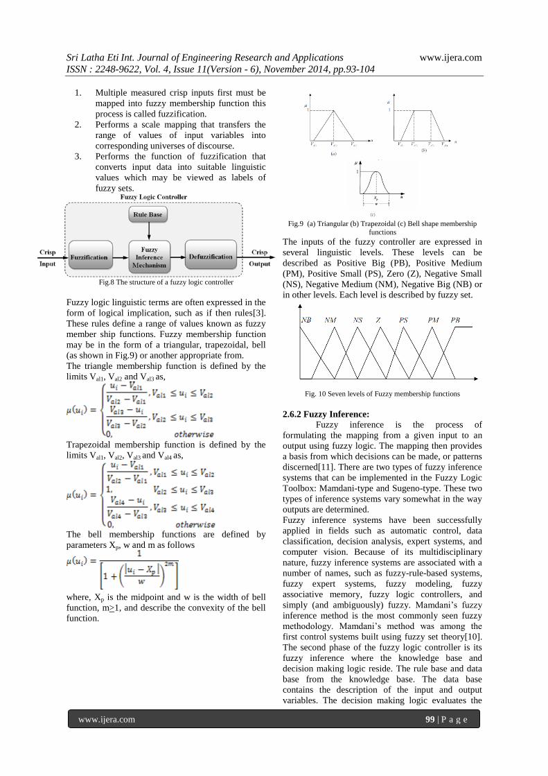
The basic structure of a fuzzy logic

controller is shown in Fig.8. Its fundamental

components are Fuzzification, control rule base,

inference mechanism and defuzzification.

2.6.1 Fuzzification:

The following functions are performed in the

Fuzzification process:




1. Multiple measured crisp inputs first must be

mapped into fuzzy membership function this

process is called fuzzification.

2. Performs a scale mapping that transfers the

range of values of input variables into

corresponding universes of discourse.

3. Performs the function of fuzzification that

converts input data into suitable linguistic

values which may be viewed as labels of

fuzzy sets.

Fig.8 The structure of a fuzzy logic controller

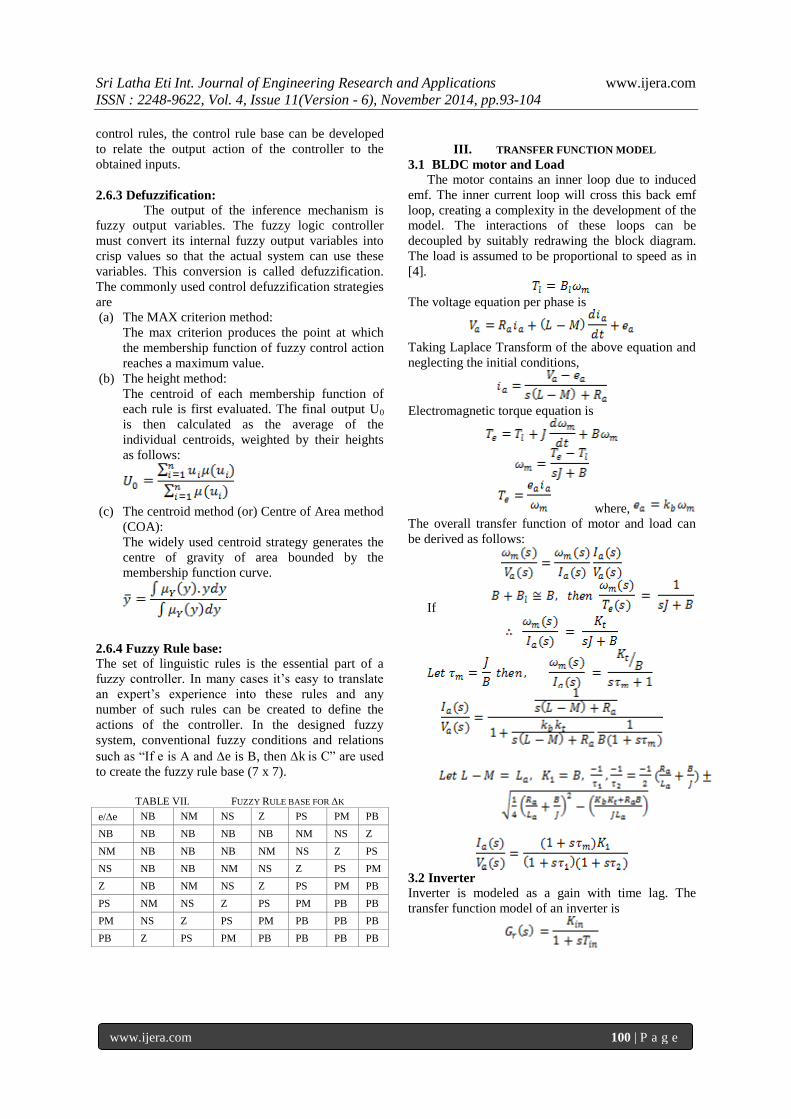
Fuzzy logic linguistic terms are often expressed in the

form of logical implication, such as if then rules[3].

These rules define a range of values known as fuzzy

member ship functions. Fuzzy membership function

may be in the form of a triangular, trapezoidal, bell

(as shown in Fig.9) or another appropriate from.

The triangle membership function is defined by the

limits Val1, Val2 and Val3 as,

Trapezoidal membership function is defined by the

limits Val1, Val2, Val3 and Val4 as,

The bell membership functions are defined by

parameters Xp, w and m as follows

where, Xp is the midpoint and w is the width of bell

function, m>1, and describe the convexity of the bell

function.

Fig.9 (a) Triangular (b) Trapezoidal (c) Bell shape membership

functions

The inputs of the fuzzy controller are expressed in

several linguistic levels. These levels can be

described as Positive Big (PB), Positive Medium

(PM), Positive Small (PS), Zero (Z), Negative Small

(NS), Negative Medium (NM), Negative Big (NB) or

in other levels. Each level is described by fuzzy set.

Fig. 10 Seven levels of Fuzzy membership functions

2.6.2 Fuzzy Inference:

Fuzzy inference is the process of

formulating the mapping from a given input to an

output using fuzzy logic. The mapping then provides

a basis from which decisions can be made, or patterns

discerned[11]. There are two types of fuzzy inference

systems that can be implemented in the Fuzzy Logic

Toolbox: Mamdani-type and Sugeno-type. These two

types of inference systems vary somewhat in the way

outputs are determined.

Fuzzy inference systems have been successfully

applied in fields such as automatic control, data

classification, decision analysis, expert systems, and

computer vision. Because of its multidisciplinary

nature, fuzzy inference systems are associated with a

number of names, such as fuzzy-rule-based systems,

fuzzy expert systems, fuzzy modeling, fuzzy

associative memory, fuzzy logic controllers, and

simply (and ambiguously) fuzzy. Mamdani’s fuzzy

inference method is the most commonly seen fuzzy

methodology. Mamdani’s method was among the

first control systems built using fuzzy set theory[10].

The second phase of the fuzzy logic controller is its

fuzzy inference where the knowledge base and

decision making logic reside. The rule base and data

base from the knowledge base. The data base

contains the description of the input and output

variables. The decision making logic evaluates the




control rules, the control rule base can be developed

to relate the output action of the controller to the

obtained inputs.

2.6.3 Defuzzification:

The output of the inference mechanism is

fuzzy output variables. The fuzzy logic controller

must convert its internal fuzzy output variables into

crisp values so that the actual system can use these

variables. This conversion is called defuzzification.

The commonly used control defuzzification strategies

are

(a) The MAX criterion method:

The max criterion produces the point at which

the membership function of fuzzy control action

reaches a maximum value.

(b) The height method:

The centroid of each membership function of

each rule is first evaluated. The final output U0

is then calculated as the average of the

individual centroids, weighted by their heights

as follows:

(c) The centroid method (or) Centre of Area method

(COA):

The widely used centroid strategy generates the

centre of gravity of area bounded by the

membership function curve.

2.6.4 Fuzzy Rule base:

The set of linguistic rules is the essential part of a

fuzzy controller. In many cases it’s easy to translate

an expert’s experience into these rules and any

number of such rules can be created to define the

actions of the controller. In the designed fuzzy

system, conventional fuzzy conditions and relations

such as “If e is A and e is B, then k is C” are used

to create the fuzzy rule base (7 x 7).

TABLE VII. FUZZY RULE BASE FOR K

e/e NB NM NS Z PS PM PB

NB NB NB NB NB NM NS Z

NM NB NB NB NM NS Z PS

NS NB NB NM NS Z PS PM

Z NB NM NS Z PS PM PB

PS NM NS Z PS PM PB PB

PM NS Z PS PM PB PB PB

PB Z PS PM PB PB PB PB

III. TRANSFER FUNCTION MODEL

3.1 BLDC motor and Load

The motor contains an inner loop due to induced

emf. The inner current loop will cross this back emf

loop, creating a complexity in the development of the

model. The interactions of these loops can be

decoupled by suitably redrawing the block diagram.

The load is assumed to be proportional to speed as in

[4].

The voltage equation per phase is

Taking Laplace Transform of the above equation and

neglecting the initial conditions,

Electromagnetic torque equation is

where,

The overall transfer function of motor and load can

be derived as follows:

If

3.2 Inverter

Inverter is modeled as a gain with time lag. The

transfer function model of an inverter is




where, and

Vdc- DC link voltage input to inverter

Vcm- Maximum control voltage

fc– Switching or carrier frequency

3.3 Current loop

Hc is the current feedback gain

Using Block diagram reduction rules, the transfer

function is obtained as follows:

In order to approximate the transfer function to

second order for simple control, the following

approximations are made near the vicinity of the

crossover frequency:

Also,

Let,

Where,

On further approximations,

The overall speed control loop is then derived from

the above transfer functions using a PID speed

controller and limiter.

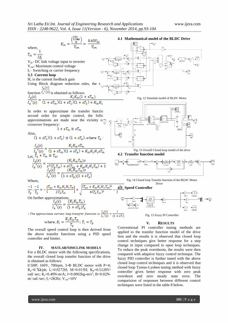
IV. MATLAB/SIMULINK MODELS For a BLDC motor with the following specifications,

the overall closed loop transfer function of the drive

is obtained as follows:

0.5HP, 160V, 700rpm, 3-Ф BLDC motor with P=4;

Ra=0.7Ω/ph; L=0.0272H; M=0.015H; Kb=0.5128V/

rad/ sec; Kt=0.49N-m/A; J=0.0002kg-m/s2; B=0.02N-

m/ rad /sec; fc=2KHz; Vcm=10V

4.1 Mathematical model of the BLDC Drive

Fig. 12 Simulink model of BLDC Motor

Fig. 13 Overall Closed loop model of the drive

4.2 Transfer function model

Fig. 14 Closed loop Transfer function of the BLDC Motor

Drive

4.3 Speed Controller

Fig. 15 Fuzzy PI Controller

V. RESULTS Conventional PI controller tuning methods are

applied to the transfer function model of the drive

first and the results it is observed that closed loop

control techniques give better response for a step

change in input compared to open loop techniques.

To reduce the peak overshoots, the results were then

compared with adaptive fuzzy control technique. The

fuzzy PID controller is further tuned with the above

closed loop control techniques and it is observed that

closed loop Tyreus-Lyuben tuning method with fuzzy

controller gives better response with zero peak

overshoot and zero steady state error. The

comparision of responses between different control

techniques were listed in the table 8 below.




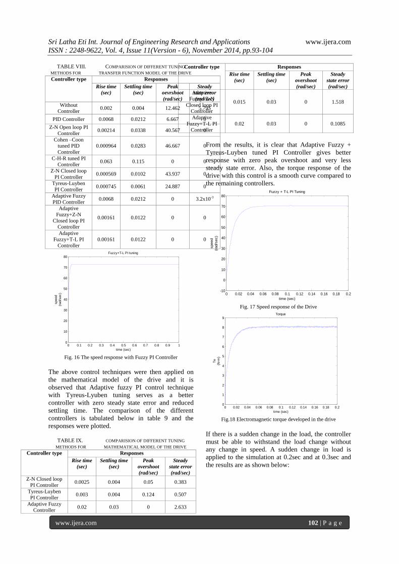
TABLE VIII. COMPARISION OF DIFFERENT TUNING

METHODS FOR TRANSFER FUNCTION MODEL OF THE DRIVE

Controller type Responses

Rise time

(sec)

Settling time

(sec)

Peak

oevrshoot

(rad/sec)

Steady

state error

(rad/sec)

Without Controller

0.002 0.004 12.462 5.795

PID Controller 0.0068 0.0212 6.667 0

Z-N Open loop PI

Controller 0.00214 0.0338 40.567 0

Cohen –Coon tuned PID

Controller

0.000964 0.0283 46.667 0

C-H-R tuned PI Controller

0.063 0.115 0 0

Z-N Closed loop

PI Controller 0.000569 0.0102 43.937 0

Tyreus-Luyben

PI Controller 0.000745 0.0061 24.887 0

Adaptive Fuzzy

PID Controller 0.0068 0.0212 0 3.2x10-3

Adaptive

Fuzzy+Z-N

Closed loop PI Controller

0.00161 0.0122 0 0

Adaptive

Fuzzy+T-L PI Controller

0.00161 0.0122 0 0

0 0.1 0.2 0.3 0.4 0.5 0.6 0.7 0.8 0.9 10

10

20

30

40

50

60

70

80

time (sec)

speed

(rad/s

ec)

Fuzzy+T-L PI tuning

Fig. 16 The speed response with Fuzzy PI Controller

The above control techniques were then applied on

the mathematical model of the drive and it is

observed that Adaptive fuzzy PI control technique

with Tyreus-Lyuben tuning serves as a better

controller with zero steady state error and reduced

settling time. The comparison of the different

controllers is tabulated below in table 9 and the

responses were plotted.

TABLE IX. COMPARISION OF DIFFERENT TUNING

METHODS FOR MATHEMATICAL MODEL OF THE DRIVE


Rise time

(sec)

Settling time

(sec)

Peak

overshoot

(rad/sec)

Steady

state error

(rad/sec)

Z-N Closed loop PI Controller

0.0025 0.004 0.05 0.383

Tyreus-Luyben

PI Controller 0.003 0.004 0.124 0.507

Adaptive Fuzzy Controller

0.02 0.03 0 2.633


Rise time

(sec)

Settling time

(sec)

Peak

overshoot

(rad/sec)

Steady

state error

(rad/sec)

Adaptive

Fuzzy+Z-N

Closed loop PI Controller

0.015 0.03 0 1.518

Adaptive

Fuzzy+T-L PI

Controller

0.02 0.03 0 0.1085

From the results, it is clear that Adaptive Fuzzy +

Tyreus-Luyben tuned PI Controller gives better

response with zero peak overshoot and very less

steady state error. Also, the torque response of the

drive with this control is a smooth curve compared to

the remaining controllers.

0 0.02 0.04 0.06 0.08 0.1 0.12 0.14 0.16 0.18 0.2-10

0

10

20

30

40

50

60

70

80

time (sec)

speed

(rad/s

ec)

Fuzzy + T-L PI Tuning

Fig. 17 Speed response of the Drive

0 0.02 0.04 0.06 0.08 0.1 0.12 0.14 0.16 0.18 0.20

1

2

3

4

5

6

7

8

9

time (sec)

Te

(N-m

)

Torque

Fig.18 Electromagnetic torque developed in the drive

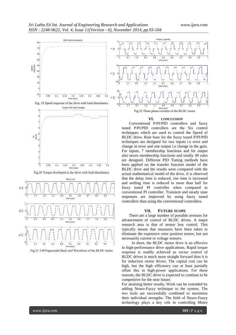
If there is a sudden change in the load, the controller

must be able to withstand the load change without

any change in speed. A sudden change in load is

applied to the simulation at 0.2sec and at 0.3sec and

the results are as shown below:




0 0.05 0.1 0.15 0.2 0.25 0.3 0.35 0.4-10

0

10

20

30

40

50

60

70

80

time (sec)

speed

(rad/s

ec)

With load disturbance

Fig. 19 Speed resposne of the drive with load disturbance

0 0.05 0.1 0.15 0.2 0.25 0.3 0.35 0.40

1

2

3

4

5

6

7

8

9

time (sec)

Te

(N-m

)

Torque with load changes

Fig.20 Torque developed in the drive with load disturbance

Fig.21 3-ФTrapezoidal Back emf Waveform of the BLDC motor

Fig.22 Three phase currents of the BLDC motor

VI. CONCLUSION

Conventional P/PI/PID controllers and fuzzy

tuned P/PI/PID controllers are the Six control

techniques which are used to control the Speed of

BLDC drive. Rule base for the fuzzy tuned P/PI/PID

techniques are designed for two inputs i.e error and

change in error and one output i.e change in the gain.

For inputs, 7 membership functions and for output

also seven membership functions and totally 49 rules

are designed. Different PID Tuning methods have

been applied on the transfer function model of the

BLDC drive and the results were compared with the

actual mathematical model of the drive. It is observed

that the delay time is reduced, rise time is increased

and settling time is reduced to more than half for

fuzzy tuned PI controller when compared to

conventional PI controller. Transient and steady state

responses are improved by using fuzzy tuned

controllers than using the conventional controllers.

VII. FUTURE SCOPE There are a large number of possible avenues for

advancement of control of BLDC drives. A major

research area is that of sensor less control. This

typically means that measures have been taken to

eliminate the expensive rotor position sensor, but not

necessarily current or voltage sensors.

In short, the BLDC motor drive is an effective

in high-performance drive applications. Rapid torque

response is readily achieved as vector control of

BLDC drives is much more straight forward than it is

for induction motor drives. The capital cost can be

high, but the high efficiency can at least partially

offset this in high-power applications. For these

reasons, the BLDC drive is expected to continue to be

competitive for the near future.

For attaining better results, Work can be extended by

adding Neuro-Fuzzy technique to the system. The

two tools are successfully combined to maximize

their individual strengths. The field of Neuro-Fuzzy

technology plays a key role in controlling Motor




drives. The present work is concluded with

sophisticated applications of BLDC drive control.

REFERENCES [1.] Padmaraja Yedamale, “Brushless DC

(BLDC) Motor Fundamentals”, Microchip

Technology Inc.

[2.] Mehmet Cunkas and Omer Aydogdu,

“Realization of fuzzy logic controlled

brushless dc motor drives using Matlab /

Simulink”, Mathematical and Computational

Applications, Vol. 15, No. 2, pp. 218-229,

2010. Association for Scientific Research.

[3.] S.Rambabu and Dr. B. D. Subudhi,

“Modeling And Control Of A Brushless DC

Motor”, National Institute of Technology,

Rourkela.

[4.] R. Krishnan, “Electric motor drives, modeling

analysis and control”, Prentice Hall

publications.

[5.] B.K. Bose, “Modern Power Electronics and

A.C Drives”, Prentice Hall PTR publications.

[6.] Dennis Fewson, “Introduction to Power

Electronics”, Essential Electronics Series.

[7.] Module 5, DC to AC Converters Version 2

EE IIT, Kharagpur

[8.] BLDC Motor Modelling and Control – A

Matlab/Simulink Implementation” by Stefan

Baldursson, International masters program in

Electric Power Engineering, Chalmers

University.

[9.] Madhusudan Singh and Archna Garg,

“Performance Evaluation of BLDC Motor

with Conventional PI and Fuzzy Speed

Controller”, Electrical Engineering

Department, Delhi Technological University.

[10.] Chuen Chien Lee, “Fuzzy Logic in Control

Systems-Fuzzy Logic Controllers”, Student

Member, IEEE, IEEE Transcations on

systems, Man, and Cybernetics, Vol.20, No.2,

March/April 1990.

[11.] Pooja Agarwal and Arpita Bose, “Brushless

Dc Motor Speed Control Using Proportional-

Integral And Fuzzy Controller”, IOSR Journal

of Electrical and Electronics Engineering

(IOSR-JEEE) e-ISSN: 2278-1676,p-ISSN:

2320-3331, Volume 5, Issue 5 (May. - Jun.

2013), PP 68-78

[12.] Jan Jantzen, “Tuning Of Fuzzy PID

Controllers”, Technical University of

Denmark, Department of Automation, Bldg

326, DK-2800 Lyngby, DENMARK. Tech.

report no 98-H 871 (fpid), April 16, 1999.

[13.] “High Performance Drives -- speed and

torque regulation” Technical Guide No.100,

ABB Industrial Systems Inc., New Berlin,

USA

Documents

Closed Loop Speed Control of a BLDC Motor Drive Using ... - 6/O04110693104.pdf · Closed Loop Speed Control of a BLDC Motor Drive Using Adaptive Fuzzy Tuned PI Controller Sri