Closed Form Solutions of Unsteady Two Fluid Flow in a Tube

Applications and Applied Mathematics: An International Applications and Applied Mathematics: An International

Journal (AAM) Journal (AAM)

Volume 14 Issue 1 Article 41

6-2019

Closed Form Solutions of Unsteady Two Fluid Flow in a Tube Closed Form Solutions of Unsteady Two Fluid Flow in a Tube

J. Liu Michigan State University

C. Y. Wang Michigan State University

Follow this and additional works at: https://digitalcommons.pvamu.edu/aam

Part of the Biology Commons, Fluid Dynamics Commons, and the Other Physical Sciences and

Mathematics Commons

Recommended Citation Recommended Citation Liu, J. and Wang, C. Y. (2019). Closed Form Solutions of Unsteady Two Fluid Flow in a Tube, Applications and Applied Mathematics: An International Journal (AAM), Vol. 14, Iss. 1, Article 41. Available at: https://digitalcommons.pvamu.edu/aam/vol14/iss1/41

This Article is brought to you for free and open access by Digital Commons @PVAMU. It has been accepted for inclusion in Applications and Applied Mathematics: An International Journal (AAM) by an authorized editor of Digital Commons @PVAMU. For more information, please contact [email protected].

https://digitalcommons.pvamu.edu/aam

https://digitalcommons.pvamu.edu/aam

https://digitalcommons.pvamu.edu/aam/vol14

https://digitalcommons.pvamu.edu/aam/vol14/iss1

https://digitalcommons.pvamu.edu/aam/vol14/iss1/41

https://digitalcommons.pvamu.edu/aam?utm_source=digitalcommons.pvamu.edu%2Faam%2Fvol14%2Fiss1%2F41&utm_medium=PDF&utm_campaign=PDFCoverPages

http://network.bepress.com/hgg/discipline/41?utm_source=digitalcommons.pvamu.edu%2Faam%2Fvol14%2Fiss1%2F41&utm_medium=PDF&utm_campaign=PDFCoverPages




https://digitalcommons.pvamu.edu/aam/vol14/iss1/41?utm_source=digitalcommons.pvamu.edu%2Faam%2Fvol14%2Fiss1%2F41&utm_medium=PDF&utm_campaign=PDFCoverPages

mailto:[email protected]

586

Closed-Form Solutions of Unsteady Two-Fluid Flow in a Tube

J. Liu and C.Y. Wang

Department of Mathematics

Michigan State University

East Lansing, MI 48824

E-mail: [email protected]

Received: July 5, 2018; Accepted: September 27, 2018

Abstract

Exact closed-form solutions for the mathematical model of unsteady two-fluid flow in a

circular tube are presented. The pressure gradient is assumed to be oscillatory or

exponentially increasing or decreasing in time. The instantaneous velocity profiles and

flow rates depend on the size of the core fluid, the density ratio, the viscosity ratio, and a

parameter (e.g. the Womersley number) quantifying time changes. Applications include

blood flow in small vessels.

Keywords: Exact solution; Viscous flow; Two-fluid; Unsteady; Blood flow

MSC 2010 No.: 76Z05, 76D50, 92C35

1. Introduction

Viscous flow in a tube is fundamental in fluid mechanics. In some cases the fluid is not

homogeneous but can be well-modeled by two different immiscible homogeneous fluids,

i.e., a core fluid and a boundary fluid. Practical examples include lubricated walls in food

processing, micro-fluidic super-hydrophobic liquid flow due to a layer of trapped gas, and

fluids with particulate suspensions, especially blood flow in small vessels.

The steady, two fluid layer channel flow, important in transport processes in chemical

engineering, was solved by Bird et al. (2007). It was extended to starting flow by Wang

(2017), exponentially increasing unsteady flow by Kapur and Shukla (1964), and

oscillatory flow by Bhattacharyya (1968). The last two references considered the special

case where the two fluid layers were of exactly the same thickness.

Available at

http://pvamu.edu/aam

Appl. Appl. Math.

ISSN: 1932-9466

Vol. 14, Issue 1 (June 2019), pp. 586 - 601

Applications and Applied

Mathematics:

An International Journal

(AAM)

1

Liu and Wang: Closed Form Solutions of Unstea dy Two Fluid Flow in a Tube

Published by Digital Commons @PVAMU, 2019

mailto:[email protected]

http://pvamu.edu/aam

AAM: Intern. J., Vol. 14, Issue 1 (June 2019) 587

The steady concentric two-fluid tube flow was first proposed by Vand (1948) for the flow

of ink suspension in tubes. Hayes (1960) and Sharan and Popel (2001) successfully

applied the two-fluid model to blood flow in small vessels. Notable extensions include

the application to stenotic vessels (Shukla et al. 1980), non-Newtonian core fluid

(Srivastava and Saxena 1994), and curved vessels (Wang and Bassingthwaighte 2003).

The model also describes the laminar transport of oil with a lubricating envelope of water

(Martinez-Palou et al. 2011). There seems to be very few unsteady two-fluid flow

solutions. Bugliarello and Sevilla (1970) formulated the pulsatile (oscillatory) flow

problem but did not give the solution or any results. The purpose of the present paper is to

present the (only two) unsteady closed-form solutions of two-fluid tube flow. These exact

solutions also serve as benchmarks for approximate methods, such as numerical, series,

or perturbation results. The properties of these solutions are important not only to the

afore-mentioned engineering applications but also to blood flow in small vessels.

Modeling blood flow in the circulation primarily depends on the diameter of the blood

vessel (relative to the size of the suspended red blood cells). It is generally accepted that

for large blood vessels blood can be considered as a homogeneous fluid with a viscosity

about 3-4 times that of water. If the vessel diameter is between 1-2 mm, blood could be

modeled by a two-phase fluid where blood and plasma have separate dynamics (e.g.,

Chow 1975, Srivastava and Srivastava 1983). If the size of the blood vessel is less than

1000 microns (1 mm) and down to 40 microns, the apparent viscosity decreases. This

phenomenon, or Fahraeus-Lindqvist effect, can be explained by the steric hindrance of

the red blood cells near the wall, where a less viscous, relatively cell-free plasma layer

exists (Pries et al. 1996). For this range of vessel diameters, it is natural to use the

two-fluid model to describe blood flow. Wang and Bassingthwaighte (2003) successfully

curve-fitted the the two-fluid theory with the experimental data of Pries (1996) and

Secomb (1995) for various hematocrit contents. It is found that nonlinear effects such as

shear dependence, rouleaux formation, wall deformation, cell deformation etc are

contained in the curve fit. For vessel diameters less than 10 microns, the apparent

viscosity increases due to the resistance of individual (now comparable in size) red blood

cells. Thus the present work shall be applicable to blood flow in vessels of 40-1000

microns in diameter.

2. Formulation

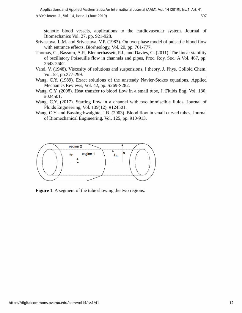
First we formulate the generic unsteady axisymmetric two-fluid problem. Figure 1 shows

a section of the long tube where region 1 is the core fluid and region 2 is the annular

boundary fluid. The Navier-Stokes equation for parallel flow degenerates to

'

''

'''

'1

'

' 11

1

1

r

ur

rrz

p

t

u

, (1)

'

''

'''

'1

'

' 22

2

2

r

ur

rrz

p

t

u

. (2)

2

Applications and Applied Mathematics: An International Journal (AAM), Vol. 14 [2019], Iss. 1, Art. 41


588 J. Liu and C.Y. Wang

Here u' is axial velocity in the axial z' direction, t' is the time, p is the pressure, is the

density, is the kinematic viscosity, and r' is the radial coordinate. The primes mean

dimensional quantities and the subscripts indicate the region. An unsteady pressure

gradient of magnitude 0G is applied.

)'('

'0 tgG

dz

dp . (3)

Normalizing all lengths by the tube radius a, the time by 1

2 /a , the velocity by

)/( 110

2 Ga and dropping primes, equations (1) and (2) reduce to

rrugu rrt /)( 11 , r0 , (4)

rrugu rrt /)( 2

2

2

, 1 r . (5)

Here, (<1) is the normalized core radius,

21

2

21 /,/ , (6)

are density and kinematic viscosity ratios. The boundary conditions are that the velocity

is bounded on the axis, no slip on the wall and velocities and shear stresses match on the

interface at r :

21 uu , (7)

rr uu 21

2 . (8)

We shall consider the two cases which yield closed-form solutions, that when the pressure

gradient is oscillatory, and when the pressure gradient is exponential in time.

3. Oscillatory flow For oscillatory flow, let

tisti eeg

2' , (9)

1

2 / as , (10)

where is the dimensional frequency, 1i , s is the Womersley number, and only

the real part of any physical term has significance. Let

)(),( 2211

22

rfeurfeu tistis . (11)

Equations (4) and (5) reduce to

3




1'1

'' 1

2

11 fisfr

f , (12)

2

2

22

22 '1

'' fisfr

f . (13)

The solutions satisfying boundedness on the axis and zero on the wall is

)(1 0121 ksrJCs

if

, (14)

)(

)(

)(

)()1(1

0

02

0

0222

ksY

rksYC

ksJ

rksJC

s

if . (15)

Here, 2/)1( ik , 0J and 0Y are Bessel functions of the first and second kind, and

21, CC are constants to be determined by equations (7,8). We find

1 1 0 0

1 0 0 1

2 0 1 0 1

0 1 0 1

1 1 0 0 0 0

0

{ ( )[( 1) ( ) ( )]

( )[( 1) ( ) ( )]} / ,

{[ ( 1) ( ) ( ) ( ) ( )

( ) ( )] ( )} / ,

( )[ ( ) ( ) ( ) ( )]

( )[

C J ks Y ks Y ks

Y ks J ks J ks

C J ks J ks J ks J ks

J ks J ks Y ks

J ks J ks Y ks Y ks J ks

J ks

0 1 0 1( ) ( ) ( ) ( )].Y ks J ks J ks Y ks

(16)

For a single fluid, one can set 1 or 1 . The solution degenerates to

)(

)(1

0

0

2

2

ksJ

ksrJ

is

eu

tis

. (17)

This is the solution of the oscillatory single-fluid flow in a circular tube found by Sexl

(1930).

The steady-state solution of the two-fluid flow can be obtained by letting s = 0 and

solving equations (12) and (13). We find the velocity profile is composed of two different

paraboloids,

])1([4

1 2222

10 ru , (18)

)1(4

22

20 ru

. (19)

This steady-state solution agrees with all previous reports. Although our equations (14)

and (15) do not directly accept s = 0, the steady-state solution can be recovered by taking

the analytic limit 0s , or evaluating numerically by letting s to be a small number,

4




such as 0001.0s . The steady-state flow rate is

)]1([8

22 424

1

20

0

100

rdrurdruQ . (20)

Note that for 1 , or for 2 =1, the two-fluid steady-state solution reduces to the

well-known single-fluid Poiseuille solution.

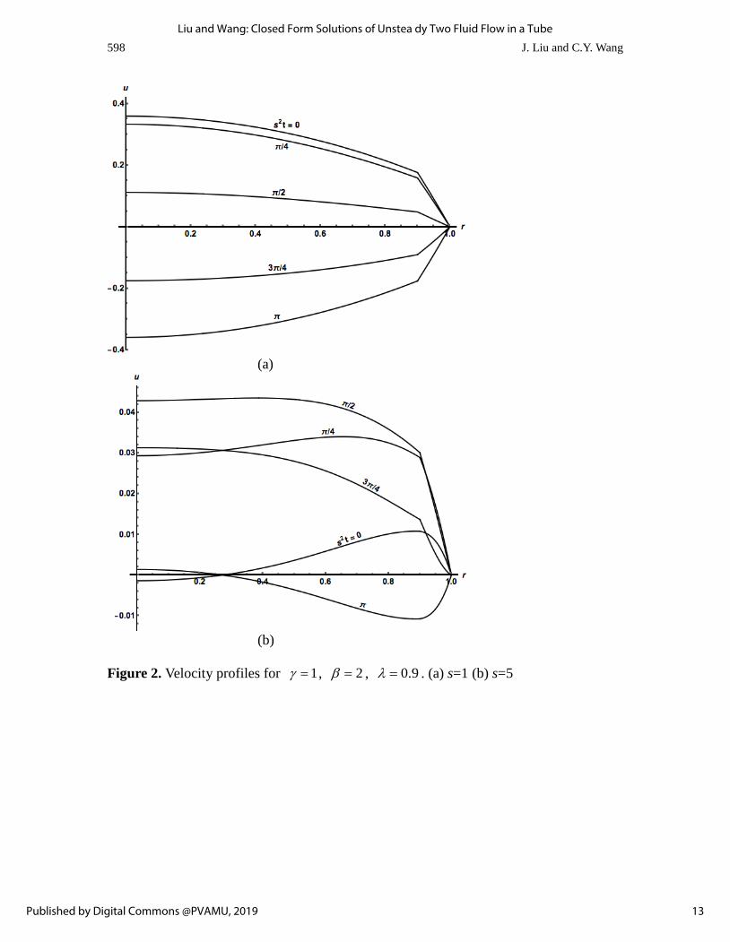
Figure 2 shows some typical oscillatory velocity profiles. The velocity is composed of

two parts, discontinuous in slope at the interface, and its magnitude is oscillatory. It is

seen that at low Womersley number s, the velocity profile is similar to the steady-state

case, with maximum on the axis of the tube. However, for s large, the maximum velocity

moved closer to the walls. This phenomenon, called the "annular effect", also exists for

single-fluid oscillatory flows (see e.g., Schlichting and Gersten 2000).

The instantaneous flow rate is

)sin()cos(22 2

2

2

1

1

2

0

1 tsEtsErdrurdruQ

. (21)

The amplitude A and the phase lag P of the flow rate are

2

2

2

1 EEA and )/(tan 12

1 EEP . (22)

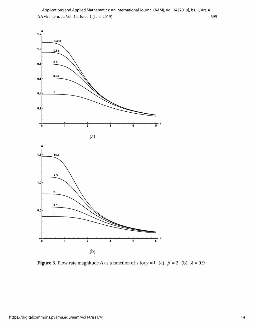
Figure 3 shows the amplitude decays from the steady state value to zero as frequency is

increased. The effect of increased core diameter is to decrease the amplitude, while

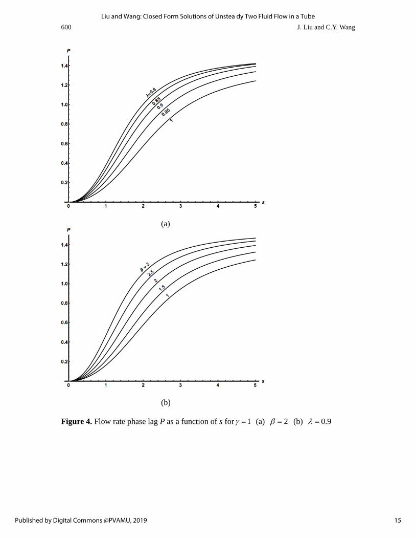
increased viscosity ratio increases the amplitude. Figure 4 shows the phase of the

oscillatory flow rate lags behind the oscillatory pressure. The phase lag is small for low

frequencies, but increases to 2/ for large frequencies. Also shown are the effects of

and .

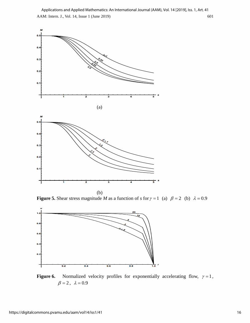
Also of interest is the shear stress on the wall. The shear stress, normalized by 0aG , is

),1(1 2

2t

r

u

. (23)

The magnitude of the shear stress

2

2 )1('

fM , (24)

is plotted in Figure 5. We see that an increase in or a decrease in increases the

5




shear stress. Increased shear stress retards accumulation of deposits, such as

atherosclerosis in vascular vessels.

4. Exponential Acceleration or Deceleration

Another closed-form solution is possible when the unsteady pressure gradient is

exponentially growing or decaying in time. Let b > 0 be a measure of the rate of increase

or decrease

tbt eeg

2' , 1

2 / ba . (25)

Here, the top sign is for increasing pressure gradient and the bottom sign is for decreasing

pressure gradient. Let

)(),( 2211

22

rheurheu tt . (26)

Equations (4) and (5) reduce to

1'1

'' 1

2

11 hhr

h , (27)

2

2

22

22 '1

'' hhr

h . (28)

The solution for the case of increasing pressure gradient is

)(11

0121 rIBh

, (29)

)(

)(

)(

)()1(1

0

02

0

0222

K

rKB

I

rIBh . (30)

Here, 0I and 0K are modified Bessel functions. The matching conditions, then,

determine the constants, i.e.,

1 1 0 0

1 0 0 2

2 0 0 1

0 1 0 1 2

2 1 0 0 0 0

0 0 1 0

{ ( )[( 1) ( ) ( )]

( )[( 1) ( ) ( )]} / ,

( )[( 1) ( ) ( )

( ) ( ) ( ) ( )] / ,

( )[ ( ) ( ) ( ) ( )]

( )[ ( ) ( ) ( )

B I K K

K I I

B K I I

I I I I

I I K K I

I I K K I

1( )].

(31)

Figure 6 shows the velocity profiles, here normalized by the maximum velocity which

occurs on the axis. When the acceleration parameter is zero, the velocity profile is

6




that of the steady-state solution. As increases, the velocity profile becomes more

blunted. For different times, the velocity profiles are similar, i.e., as time increases the

magnitudes increase exponentially. The instantaneous flow rate is

2

2 0 1 1

2 0 1 1

2 2

0 0

3

1 1 0 0

2 {2( 1) ( )[ ( ) ( )]

2 ( )[ ( ) ( )]

( ) ( )[ ( )

2 ( )]} / [2 ( ) ( )].

tQ e B K I I

B I K K

I K

B I I K

(32)

In the case of a single fluid with exponentially increasing pressure gradient, our solution

reduces to

)(

)(1

0

0

2

2

I

rIeu

t

. (33)

This exact solution agrees with that of Sanyal (1956).

For the exponentially decreasing pressure gradient, we find

)(11

0121 rJDh

, (34)

)(

)(

)(

)()1(1

0

02

0

0222

Y

rYD

J

rJDh , (35)

1 1 0 0

1 0 0 3

2 0 1 0 0

0 1 3

3 1 0 0 0 0

0 0 1 0 1

{ ( )[( 1) ( ) ( )]

( )[( 1) ( ) ( )]} / ,

( ){ ( )[( 1) ( ) ( )]

( ) ( )} / ,

( )[ ( ) ( ) ( ) ( )]

( )[ ( ) ( ) ( ) (

D J Y Y

Y J J

D Y J J J

J J

J J Y Y J

J Y J J Y

)].

(36)

In the case of a single fluid, put 1 or 1 , and the solution becomes

)(2

rheu t ,

)(

)(1

1

0

0

2

J

rJh . (37)

Equation (37) reduces to the paraboloidal Poiseuille velocity when =0. However, it

fails when is increased to 2.4048, or the first zero of 0J . This is because the velocity

can no longer be described by the same exponential decay as the pressure gradient. The

solution should be replaced by

7




)()1()()()1(

0102

2

rJcGrGrtJG

eu

t

, (38)

)()()()()(4

)( 10011

2

rYrJrYrJrJr

rG

. (39)

Note that there is a homogeneous solution with arbitrary constant 1c which depends on

the initial conditions, and the existence of a slower decay tte2 term. We shall limit

equation (37) to 0 < < 2.4048, since for large values the pressure decrease is too

precipitous to be practical. For example, experimental measurements after the occlusion

of 100 micron microvessels show the pressure decreased with two slowly decaying

exponentials of = 0.028 and 0.079, (Maarek et al. 1990).

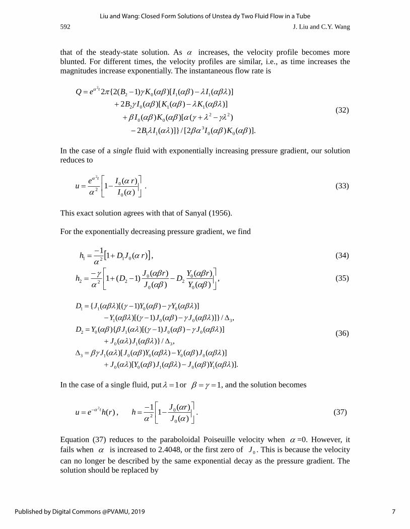
For two-fluid flow, the exact solution equations (26), (34) and (35) is also limited in the

deceleration rate. The upper limit range for the exponent is found from the zero of the

denominator of the coefficient 1D given in Table 1.

Table 1. Upper limit for deceleration exponent for the case 1

\ 1 1.5 2 2.5 3

0.8 2.4048 1.9305 1.5615 1.2953 1.1011

0.85 2.4048 2.0108 1.6802 1.4159 1.2148

0.9 2.4048 2.1287 1.8450 1.5966 1.3930

0.95 2.4048 2.2586 2.0800 1.8923 1.7133

1 2.4048 2.4048 2.4048 2.4048 2.4048

The decelerating velocity profiles for the admissible ranges are similar to the

steady-state profiles and are not presented here. The instantaneous flow rate is

2

2 0 1 1

2 0 1 1

2 2

0 0

3

1 1 0 0

2 {2(1 ) ( )[ ( ) ( )]

2 ( )[ ( ) ( )]

( ) ( )[ ( )

2 ( )]} / [2 ( ) ( )].

tQ e D Y J J

D J Y Y

J Y

D J J Y

(40)

5. Discussion

Axisymmetric two-fluid flow in a tube is also called core-annular flow, important in the

transport of viscous liquids such as oil. The steady core-annular flow has been studied by

many authors, both theoretically (for stability) and experimentally. The existence of a

stable core-annular flow depends on the inner diameter of the tube, the diameter of the

core fluid, the densities, viscosities and velocities of the two fluids, the material and

smoothness of the wall, the orientation with respect to gravity, and whether surfactants

are added. See the review of Ghosh et al. (2009) for the details.

8




We are interested in the two-fluid tube flow and its applications to blood flow. As

mentioned before, experimental blood flow properties such as velocity and resistance

(including the Fahraeus-Lindqvist effect) in the microvasculature can be predicted by the

two-fluid model. The parameter ranges for which the two-fluid model is applicable are as

follows: the (inner) vessel diameter between 40-1000 microns, the hematocrit between

15% to 60%, the ratio of the core diameter to the vessel diameter between 0.82 to 1, and

the ratio of core viscosity to plasma viscosity between 1.5 to 5. See Wang and

Bassingthwaighte (2003) and Wang (2008) for the justification of using the two-fluid

model in explaining the experimental results.

The pressure gradient of our analysis is assumed to be either sinusoidal or exponential in

time. In practice the pressure gradient may be pulsatile, which can be decomposed into a

steady part and an oscillatory part. The oscillatory part may be further Fourier

decomposed to a sum of single harmonics. For example, we found a typical pressure

measurement in a venule (e.g., Gaehtgens 1970) can be very accurately represented by a

constant and several sinusoidal harmonics, each with its own amplitude and phase.

Aside from geometric factors, oscillatory flow is governed by the Womersley number s in

equation (10). For normal blood flow in arterioles of 100 micron diameter, and a resting

frequency of 60 beats per minute, we find the (dominant harmonic) s is about 0.1. The

value of s is about 1 for birds with a heart beat of 900 beats per minute. The s value for

the higher harmonics may be several times larger.

The exponentially growing or exponentially decaying solutions model increased or

decreased pressure gradient as in opening or closing a valve or a sphincter. These results

are quite different from those of the oscillatory flow. These exponential solutions can also

be superposed. For example, it was found that micro-vascular pressure measurements

decays after an arterial occlusion. This pressure decay can be described by the sum of two

exponentials (Pellett et al. 1999). Then using our analysis, the velocity, flow and stress

properties (which are difficult to measure) can be predicted.

In order to maintain the interface between the two fluids, gravity effects must not be

important, or the density ratio is close to one. This is indeed true for suspensions such

as ink or blood. To illustrate, it takes much effort by ultracentrifuge to separate plasma

from whole blood. Thus in normal circumstances the interface is maintained.

Our exact solutions may be limited by stability. Using a perturbation on the exact

solutions found in this paper, the resulting Orr-Sommerfeld equation can be analyzed

using Floquet theory (for oscillatory flow) and/or numerical integration. This has not

been done due to the limited aims of the present paper. However, some conclusions about

stability can be made from existing reports as follows.

Oscillatory tube flow is governed by an oscillatory Reynolds number defined as

9




2Re

U , (41)

where U is the maximum oscillatory velocity. Typical experimental observations in a

cat venule of 78 micron diameter yield a maximum velocity about 10.67 0.33 cm/sec at

a frequency of 2.5 beats/sec (Intaglietta et al. 1971). Using these values we find Re=0.37

from Equation (41). The steady through-flow Reynolds number is also small, about 3.34.

Thomas et al. (2011) used linear stability theory on single-fluid oscillatory tube flow.

They found the critical oscillatory Reynolds number to be 600-700, which is two or three

times the experimentally measured values. The addition of a steady through flow

increased stability. For two-fluid tube flow, there are added stability concerns at the

interface due to differences in density, velocity and shear, aside from surface tension.

Using linear analysis, Preziosi et al. (1989) predicted the two-fluid steady tube flow is

stable for Reynolds numbers below about 100. At small Reynolds numbers the flow may

be unstable to long waves due to surface tension. However, surface tension is absent for

our two-fluid blood flow model, since the interface is due to steric hindrance instead of a

true immiscible interface. Since both oscillatory and through-flow Reynolds numbers are

of order unity (even for larger micro-vessels), we can safely conclude oscillatory (and

pulsatile) two-fluid blood flow in micro-vessels are stable.

6. Conclusions

Exact closed-form solutions of the Navier-Stokes equations are found for the unsteady

two-fluid motion in a tube.

An important parameter governing oscillatory flow is the Womersley number s. At small

s the velocity profile is composed of two paraboloids, with a kink at the interface. At

large s the velocity profile exhibits "annular effect", or its maximum moves toward the

wall. For a given oscillatory pressure, the flow rate decreases with larger s, larger core

radius fraction, and smaller viscosity ratio.

The velocity profile for exponentially accelerating flow is composed of two paraboloids

at low acceleration, but becomes flattened when the acceleration is high. On the other

hand, non-uniqueness occurs for exponentially decelerating flow, when the deceleration

exponent has the same value as the zero of the Bessel function.

Two-fluid flow in a tube is an important model for blood flow in micro-vessels of

40-1000 microns, as illustrated by the many examples. Our exact solutions may serve as a

base for future more-refined models.

REFERENCES

Bhattacharyya, R.N. (1968). Note on the unsteady flow of two incompressible

immiscible fluids between two plates, Bull. Calcutta Math. Soc. Vol.1, pp.129-136.

Bird, R.B., Stewart, W.E., and Lightfoot, E.N. (2007). Transport Phenomena, 2nd Ed.,

10




Wiley, New York.

Bugliarello, G. and Sevilla, J. (1970). Velocity distribution and other characteristics of

steady and pulsatile blood flow in fine glass tubes, Biorheology, Vol. 7, pp.85-107.

Chow, J.C.F. (1975). Blood flow: Theory, effective viscosity and effects of particle

distribution, Bulletin of Mathematical Biology, Vol. 37, pp. 471-488.

Gaehtgens, P.A.L. (1970). Pulsatile pressure and flow in the mesenteric vascular bed of

the cat. Pflugers Archiv Vol. 316, pp. 140-151.

Ghosh, S., Mandal, T.K., Das, G., and Das, P.K. (2009). Review of oil water core annular

flow, Ren. Sust. Energy Rev. Vol. 13, pp. 1957-1965.

Hayes, R.H. (1960). Physical basis of the dependence of blood viscosity on tube radius,

Am. J. Physiol. Vol. 198, pp.1193-1200.

Intaglietta, M., Richardson, D.A., and Tompkins, W.R. (1971). Blood pressure, flow, and

elastic properties in microvessels of cat omentum, Am. J. Physiol. Vol. 221, pp.

922-928.

Kapur, J.N. and Shukla, J.B. (1964). On the unsteady flow of two incompressible

immiscible fluids between two plates, Z. Angew. Math. Mech. Vol. 44(6),

pp.268-269.

Maarek, J.M.I., Hakim, T.S., and Chang, H.K. (1990). Analysis of pulmonary arterial

pressure profile after occlusion of pulsatile blood flow, J. Appl. Physiol. Vol. 68, pp.

761-769.

Martinez-Palou, R., Mosqueira, M.L., Zapata-Rendon, B., Mar-Juarez, E.,

Bernal-Huicochea, C., Clavel-Lopez, J.C. and Aburto, J. (2011). Transportation of

heavy and extra-heavy crude oil by pipeline: A review, Journal of Petroleum Science

and Engineering, Vol. 75, pp.274-282.

Pellett, A.A., Johnson, R.W., Morrison, G.G., Champagne, M.S., deBoisblanc, B.P. and

Levitzky, M.G. (1999). A comparison of pulmonary arterial occlusion algorithms for

estimation of pulmonary capillary pressure. American Journal of Respiratory and

Critical Care Medicine Vol. 160, pp. 162-168.

Preziosi, L., Chen, K., and Joseph, D.D. (1989). Lubricated pipelining: stability of

core-annular flow, J. Fluid Mech. Vol. 201, pp. 323-356.

Pries, A.R., Secomb, T.W. and Gaehtgens, P. (1996). Biophysics aspects of blood flow in

the microvasculature, Cardiovascular Research, Vol. 32, pp. 654-667.

Sanyal, L. (1956). The flow of a viscous liquid in a circular tube under pressure gradients

varying exponentially with time, Indian J. Phys. Vol. 30, pp. 57-61.

Secomb, T.W. (1995). Mechanics of blood flow in the microcirculation, in Biological

Fluid Dynamics, Eds. C.P. Ellington and T.J. Pedley, Society of Experimental

Biology, Cambridge, MA pp. 305-321.

Sexl, T. (1930). Uber den von E.G. Richardson entdeckten 'Annulareffekt', Zeit. Phys. Vol.

61, pp. 349-362.

Schlichting, H. and Gersten, K. (2000). Boundary Layer Theory, 8th Ed., Springer, Berlin.

Sharan, M. and Popel, A.S. (2001). A two-phase model for flow of blood in narrow tubes

with increased effective viscosity near the wall, Biorheology Vol.38, pp.415-428.

Shukla, J.B., Parihar, R.S. and Gupta, S.P. (1980). Effects of peripheral layer viscosity on

blood flow through the artery with mild stenosis. Bulletin of Mathematical Biology

Vol. 42, pp. 707-805.

Srivastava, V.P. and Saxena, M. (1994). Two-layered model of Casson fluid flow through

11




stenotic blood vessels, applications to the cardiovascular system. Journal of

Biomechanics Vol. 27, pp. 921-928.

Srivastava, L.M. and Srivastava, V.P. (1983). On two-phase model of pulsatile blood flow

with entrance effects. Biorheology, Vol. 20, pp. 761-777.

Thomas, C., Bassom, A.P., Blennerhassett, P.J., and Davies, C. (2011). The linear stability

of oscillatory Poiseuille flow in channels and pipes, Proc. Roy. Soc. A Vol. 467, pp.

2643-2662.

Vand, V. (1948). Viscosity of solutions and suspensions, I theory, J. Phys. Colloid Chem.

Vol. 52, pp.277-299.

Wang, C.Y. (1989). Exact solutions of the unsteady Navier-Stokes equations, Applied

Mechanics Reviews, Vol. 42, pp. S269-S282.

Wang, C.Y. (2008). Heat transfer to blood flow in a small tube, J. Fluids Eng. Vol. 130,

#024501.

Wang, C.Y. (2017). Starting flow in a channel with two immiscible fluids, Journal of

Fluids Engineering, Vol. 139(12), #124501.

Wang, C.Y. and Bassingthwaighte, J.B. (2003). Blood flow in small curved tubes, Journal

of Biomechanical Engineering, Vol. 125, pp. 910-913.

Figure 1. A segment of the tube showing the two regions.

12




(a)

(b)

Figure 2. Velocity profiles for 1 , 2 , 9.0 . (a) s=1 (b) s=5

13




(a)

(b)

Figure 3. Flow rate magnitude A as a function of s for 1 (a) 2 (b) 9.0

14




(a)

(b)

Figure 4. Flow rate phase lag P as a function of s for 1 (a) 2 (b) 9.0

15




(a)

(b)

Figure 5. Shear stress magnitude M as a function of s for 1 (a) 2 (b) 9.0

Figure 6. Normalized velocity profiles for exponentially accelerating flow, 1 ,

2 , 9.0

16



Documents

Closed Form Solutions of Unsteady Two Fluid Flow in a Tube