Closed Form Solutions

Mark van Hoeij1

Florida State University

ISSAC 2017

1Supported by NSF 16186571 / 26

What is a closed form solution?

Example: Solve this equation for y = y(x).

y ′ =4− x3

(1− x)2ex

Definition

A closed form solution is an expression for an exact solutiongiven with a finite amount of data.

This is not a closed form solution:

y = 4x + 6x2 +22

3x3 +

95

12x4 + · · ·

because making it exact requires infinitely many terms.

The Risch algorithm finds a closed form solution:

y =2 + x2

1− xex

2 / 26

Risch algorithm (1969)

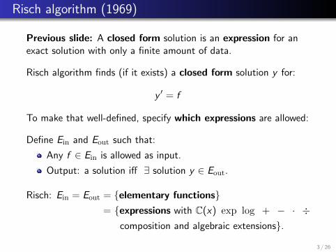
Previous slide: A closed form solution is an expression for anexact solution with only a finite amount of data.

Risch algorithm finds (if it exists) a closed form solution y for:

y ′ = f

To make that well-defined, specify which expressions are allowed:

Define Ein and Eout such that:

Any f ∈ Ein is allowed as input.

Output: a solution iff ∃ solution y ∈ Eout.

Risch: Ein = Eout = {elementary functions}= {expressions with C(x) exp log + − · ÷

composition and algebraic extensions}.

3 / 26

Liouvillian solutions

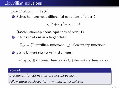
Kovacic’ algorithm (1986)

1 Solves homogeneous differential equations of order 2

a2y′′ + a1y

′ + a0y = 0

(Risch: inhomogeneous equations of order 1)

2 It finds solutions in a larger class:

Eout = {Liouvillian functions} ) {elementary functions}

3 but it is more restrictive in the input:

a0, a1, a2 ∈ {rational functions} ( {elementary functions}

Remark

∃ common functions that are not Liouvillian.

Allow those as closed form need other solvers.

4 / 26

A non-Liouvillian example

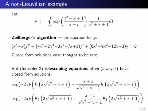
Let

y :=

∮γexp

(t2 + x + 1

x − t

)t

x2 + x + 1dt

Zeilberger’s algorithm an equation for y :

(x4−x)y ′′ + (4x4+2x3−3x2−7x+1)y ′ + (6x3−9x2−12x+3)y = 0

Closed form solutions were thought to be rare.

But (for order 2) telescoping equations often (always?) haveclosed form solutions:

exp(−2x)·(I0(

2√x2 + x + 1

)− x + 1√

x2 + x + 1I1(

2√x2 + x + 1

))exp(−2x)·

(K0

(2√x2 + x + 1

)+

x + 1√x2 + x + 1

K1

(2√x2 + x + 1

))5 / 26

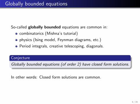
Globally bounded equations

So-called globally bounded equations are common in:

combinatorics (Mishna’s tutorial)

physics (Ising model, Feynman diagrams, etc.)

Period integrals, creative telescoping, diagonals.

Conjecture

Globally bounded equations (of order 2) have closed form solutions.

In other words: Closed form solutions are common.

6 / 26

Local to global strategy

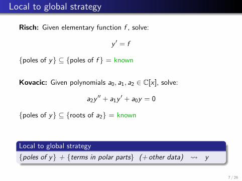
Risch: Given elementary function f , solve:

y ′ = f

{poles of y} ⊆ {poles of f } = known

Kovacic: Given polynomials a0, a1, a2 ∈ C[x ], solve:

a2y′′ + a1y

′ + a0y = 0

{poles of y} ⊆ {roots of a2} = known

Local to global strategy

{poles of y} + {terms in polar parts} (+ other data) y

7 / 26

Local data: Classifying singularities

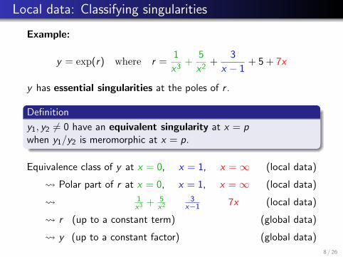
Example:

y = exp(r) where r =1

x3+

5

x2+

3

x − 1+ 5 + 7x

y has essential singularities at the poles of r .

Definition

y1, y2 6= 0 have an equivalent singularity at x = pwhen y1/y2 is meromorphic at x = p.

Equivalence class of y at x = 0, x = 1, x =∞ (local data)

Polar part of r at x = 0, x = 1, x =∞ (local data)

1x3

+ 5x2

3x−1 7x (local data)

r (up to a constant term) (global data)

y (up to a constant factor) (global data)

8 / 26

Reconstructing solutions from local data

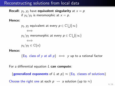
Recall: y1, y2 have equivalent singularity at x = pif y1/y2 is meromorphic at x = p.

Hence:

y1, y2 equivalent at every p ∈ C⋃{∞}

⇐⇒y1/y2 meromorphic at every p ∈ C

⋃{∞}

⇐⇒y1/y2 ∈ C(x)

Hence:

{Eq. class of y at all p} ⇐⇒ y up to a rational factor

For a differential equation L can compute:

{generalized exponents of L at p} ≈ {Eq. classes of solutions}

Choose the right one at each p a solution (up to ≈)9 / 26

Example: generalized exponents

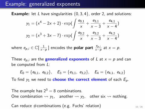
Example: let L have singularities {0, 3, 4}, order 2, and solutions:

y1 = (x4 − 2x + 2) · exp(

∫e0,1x

+e3,1x − 3

+e4,1x − 4

)

y2 = (x3 + 3x − 7) · exp(

∫e0,2x

+e3,2x − 3

+e4,2x − 4

)

where ep,i ∈ C[ 1x−p ] encodes the polar part

ep,ix−p at x = p.

These ep,i are the generalized exponents of L at x = p and canbe computed from L:

E0 = {e0,1, e0,2}, E3 = {e3,1, e3,2}, E4 = {e4,1, e4,2}To find y1 we need to choose the correct element of each Ep.

The example has 23 = 8 combinations.One combination y1, another y2, other six nothing.

Can reduce #combinations (e.g. Fuchs’ relation) 10 / 26

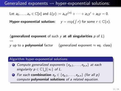
Generalized exponents hyper-exponential solutions:

Let a0, . . . , an ∈ C[x ] and L(y) := any(n) + · · ·+ a1y

′ + a0y = 0.

Hyper-exponential solution: y = exp(∫r) for some r ∈ C(x).

{generalized exponent of such y at all singularities p of L} y up to a polynomial factor (generalized exponent ≈ eq. class)

Algorithm hyper-exponential solutions:

1 Compute generalized exponents {ep,1, . . . , ep,n} at eachsingularity p ∈ C

⋃{∞} of L.

2 For each combination ep ∈ {ep,1, . . . , ep,n} (for all p)compute polynomial solutions of a related equation.

11 / 26

Same strategy for difference equation

Combine generalized exponents hyper-exponential solutions.

To do the same for difference equations we need the differenceanalogue of generalized exponents:

Difference case: p =∞ is similar to the differential case.

But a finite singularity is not an element p ∈ C.

Instead it is an element of C/Z because

y(x) singular at p ⇐⇒ y(x + 1) singular at p

is only true for p =∞.

(1997): Generalized exponents

(1999): Difference case analogue:

generalized exponents at p =∞ and

valuation growths at p ∈ C/Z Algorithm for hypergeometric solutions.

12 / 26

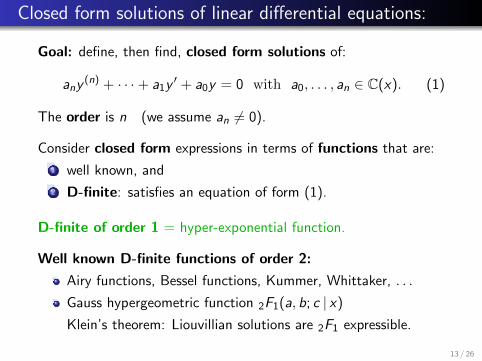
Closed form solutions of linear differential equations:

Goal: define, then find, closed form solutions of:

any(n) + · · ·+ a1y

′ + a0y = 0 with a0, . . . , an ∈ C(x). (1)

The order is n (we assume an 6= 0).

Consider closed form expressions in terms of functions that are:

1 well known, and

2 D-finite: satisfies an equation of form (1).

D-finite of order 1 = hyper-exponential function.

Well known D-finite functions of order 2:

Airy functions, Bessel functions, Kummer, Whittaker, . . .

Gauss hypergeometric function 2F1(a, b; c | x)

Klein’s theorem: Liouvillian solutions are 2F1 expressible.

13 / 26

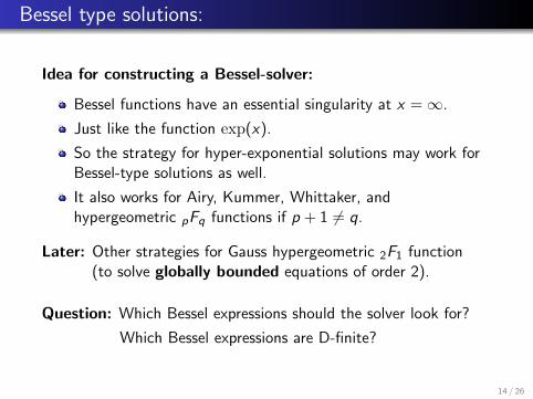
Bessel type solutions:

Idea for constructing a Bessel-solver:

Bessel functions have an essential singularity at x =∞.

Just like the function exp(x).

So the strategy for hyper-exponential solutions may work forBessel-type solutions as well.

It also works for Airy, Kummer, Whittaker, andhypergeometric pFq functions if p + 1 6= q.

Later: Other strategies for Gauss hypergeometric 2F1 function(to solve globally bounded equations of order 2).

Question: Which Bessel expressions should the solver look for?

Which Bessel expressions are D-finite?

14 / 26

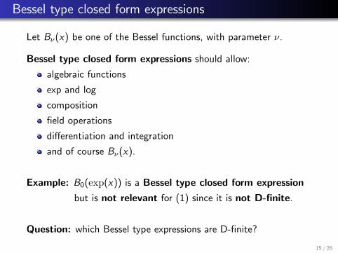
Bessel type closed form expressions

Let Bν(x) be one of the Bessel functions, with parameter ν.

Bessel type closed form expressions should allow:

algebraic functions

exp and log

composition

field operations

differentiation and integration

and of course Bν(x).

Example: B0(exp(x)) is a Bessel type closed form expression

but is not relevant for (1) since it is not D-finite.

Question: which Bessel type expressions are D-finite?

15 / 26

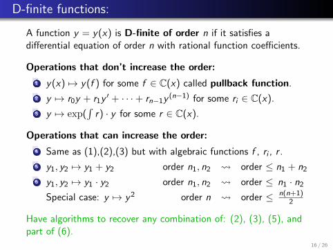
D-finite functions:

A function y = y(x) is D-finite of order n if it satisfies adifferential equation of order n with rational function coefficients.

Operations that don’t increase the order:

1 y(x) 7→ y(f ) for some f ∈ C(x) called pullback function.

2 y 7→ r0y + r1y′ + · · ·+ rn−1y

(n−1) for some ri ∈ C(x).

3 y 7→ exp(∫r) · y for some r ∈ C(x).

Operations that can increase the order:

4 Same as (1),(2),(3) but with algebraic functions f , ri , r .

5 y1, y2 7→ y1 + y2 order n1, n2 order ≤ n1 + n26 y1, y2 7→ y1 · y2 order n1, n2 order ≤ n1 · n2

Special case: y 7→ y2 order n order ≤ n(n+1)2

Have algorithms to recover any combination of: (2), (3), (5), andpart of (6).

16 / 26

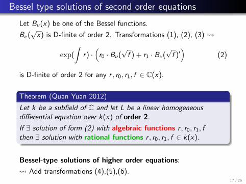
Bessel type solutions of second order equations

Let Bν(x) be one of the Bessel functions.

Bν(√x) is D-finite of order 2. Transformations (1), (2), (3)

exp(

∫r) ·(r0 · Bν(

√f ) + r1 · Bν(

√f )′)

(2)

is D-finite of order 2 for any r , r0, r1, f ∈ C(x).

Theorem (Quan Yuan 2012)

Let k be a subfield of C and let L be a linear homogeneousdifferential equation over k(x) of order 2.

If ∃ solution of form (2) with algebraic functions r , r0, r1, fthen ∃ solution with rational functions r , r0, r1, f ∈ k(x).

Bessel-type solutions of higher order equations:

Add transformations (4),(5),(6).17 / 26

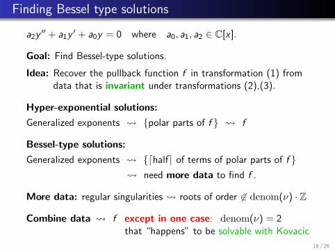
Finding Bessel type solutions

a2y′′ + a1y

′ + a0y = 0 where a0, a1, a2 ∈ C[x ].

Goal: Find Bessel-type solutions.

Idea: Recover the pullback function f in transformation (1) fromdata that is invariant under transformations (2),(3).

Hyper-exponential solutions:

Generalized exponents {polar parts of f } f

Bessel-type solutions:

Generalized exponents {dhalfe of terms of polar parts of f } need more data to find f .

More data: regular singularities roots of order 6∈ denom(ν) · Z

Combine data f except in one case: denom(ν) = 2that “happens” to be solvable with Kovacic

18 / 26

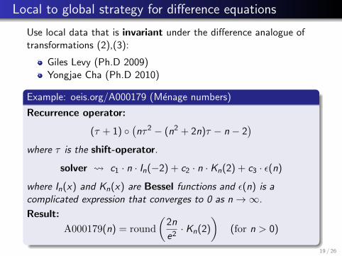
Local to global strategy for difference equations

Use local data that is invariant under the difference analogue oftransformations (2),(3):

Giles Levy (Ph.D 2009)Yongjae Cha (Ph.D 2010)

Example: oeis.org/A000179 (Menage numbers)

Recurrence operator:

(τ + 1) ◦(nτ2 − (n2 + 2n)τ − n − 2

)where τ is the shift-operator.

solver c1 · n · In(−2) + c2 · n · Kn(2) + c3 · ε(n)

where In(x) and Kn(x) are Bessel functions and ε(n) is acomplicated expression that converges to 0 as n→∞.

Result:

A000179(n) = round

(2n

e2· Kn(2)

)(for n > 0)

19 / 26

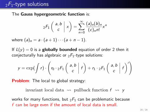
2F1-type solutions

The Gauss hypergeometric function is:

2F1

(a, bc

∣∣∣∣ x) =∞∑n=0

(a)n(b)n(c)nn!

xn

where (a)n = a · (a + 1) · · · (a + n − 1).

If L(y) = 0 is a globally bounded equation of order 2 then itconjecturally has algebraic or 2F1-type solutions:

y = exp(

∫r) ·

(r0 · 2F1

(a, bc

∣∣∣∣ f)+ r1 · 2F1(

a, bc

∣∣∣∣ f)′)

Problem: The local to global strategy:

invariant local data pullback function f y

works for many functions, but 2F1 can be problematic becausef can be large even if the amount of local data is small.

20 / 26

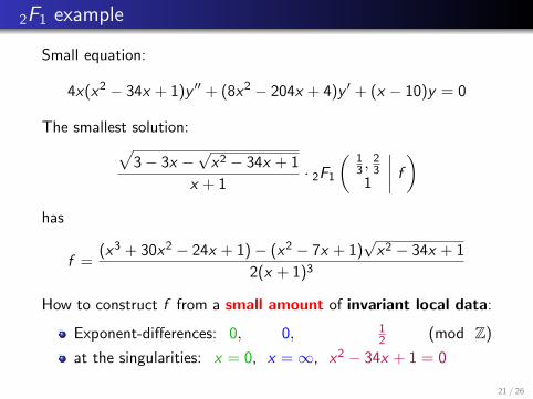
2F1 example

Small equation:

4x(x2 − 34x + 1)y ′′ + (8x2 − 204x + 4)y ′ + (x − 10)y = 0

The smallest solution:√3− 3x −

√x2 − 34x + 1

x + 1· 2F1

(13 ,

23

1

∣∣∣∣ f)has

f =(x3 + 30x2 − 24x + 1)− (x2 − 7x + 1)

√x2 − 34x + 1

2(x + 1)3

How to construct f from a small amount of invariant local data:

Exponent-differences: 0, 0, 12 (mod Z)

at the singularities: x = 0, x =∞, x2 − 34x + 1 = 0

21 / 26

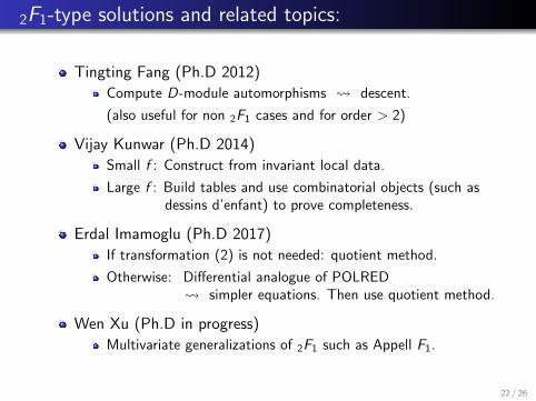
2F1-type solutions and related topics:

Tingting Fang (Ph.D 2012)

Compute D-module automorphisms descent.

(also useful for non 2F1 cases and for order > 2)

Vijay Kunwar (Ph.D 2014)

Small f : Construct from invariant local data.

Large f : Build tables and use combinatorial objects (such asdessins d’enfant) to prove completeness.

Erdal Imamoglu (Ph.D 2017)

If transformation (2) is not needed: quotient method.

Otherwise: Differential analogue of POLRED simpler equations. Then use quotient method.

Wen Xu (Ph.D in progress)

Multivariate generalizations of 2F1 such as Appell F1.

22 / 26

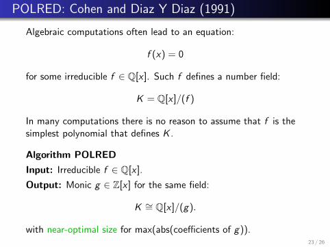
POLRED: Cohen and Diaz Y Diaz (1991)

Algebraic computations often lead to an equation:

f (x) = 0

for some irreducible f ∈ Q[x ]. Such f defines a number field:

K = Q[x ]/(f )

In many computations there is no reason to assume that f is thesimplest polynomial that defines K .

Algorithm POLRED

Input: Irreducible f ∈ Q[x ].

Output: Monic g ∈ Z[x ] for the same field:

K ∼= Q[x ]/(g).

with near-optimal size for max(abs(coefficients of g)).23 / 26

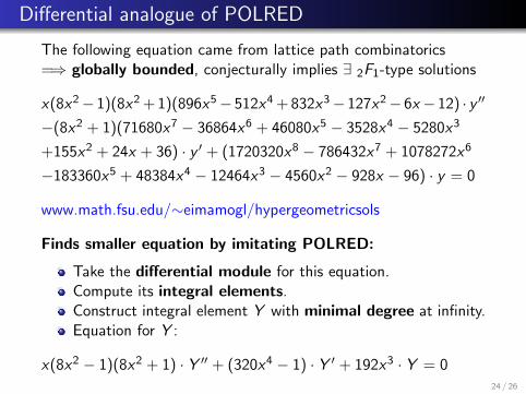
Differential analogue of POLRED

The following equation came from lattice path combinatorics=⇒ globally bounded, conjecturally implies ∃ 2F1-type solutions

x(8x2− 1)(8x2 + 1)(896x5− 512x4 + 832x3− 127x2− 6x − 12) · y ′′

−(8x2 + 1)(71680x7 − 36864x6 + 46080x5 − 3528x4 − 5280x3

+155x2 + 24x + 36) · y ′ + (1720320x8 − 786432x7 + 1078272x6

−183360x5 + 48384x4 − 12464x3 − 4560x2 − 928x − 96) · y = 0

www.math.fsu.edu/∼eimamogl/hypergeometricsols

Finds smaller equation by imitating POLRED:

Take the differential module for this equation.Compute its integral elements.Construct integral element Y with minimal degree at infinity.Equation for Y :

x(8x2 − 1)(8x2 + 1) · Y ′′ + (320x4 − 1) · Y ′ + 192x3 · Y = 024 / 26

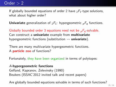
Order > 2

If globally bounded equations of order 2 have 2F1-type solutions,what about higher order?

Univariate generalization of 2F1: hypergeometric pFq functions.

Globally bounded order 3 equations need not be pFq-solvable.Can construct a univariate example from multivariatehypergeometric functions (substitution univariate).

There are many multivariate hypergeometric functions.A particle zoo of functions?

Fortunately, they have been organized in terms of polytopes:

A-hypergeometric functionsGelfand, Kapranov, Zelevinsky (1990)Beukers (ISSAC’2012 invited talk and recent papers)

Are globally bounded equations solvable in terms of such functions?25 / 26

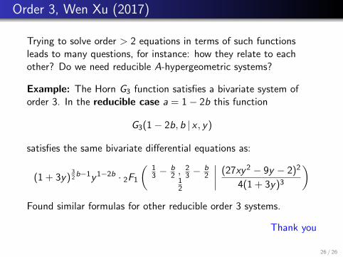
Order 3, Wen Xu (2017)

Trying to solve order > 2 equations in terms of such functionsleads to many questions, for instance: how they relate to eachother? Do we need reducible A-hypergeometric systems?

Example: The Horn G3 function satisfies a bivariate system oforder 3. In the reducible case a = 1− 2b this function

G3(1− 2b, b | x , y)

satisfies the same bivariate differential equations as:

(1 + 3y)32b−1y1−2b · 2F1

(13 −

b2 ,

23 −

b2

12

∣∣∣∣ (27xy2 − 9y − 2)2

4(1 + 3y)3

)Found similar formulas for other reducible order 3 systems.

Thank you

26 / 26