Closed-form approximations of the peak-to-average power

HAL Id: hal-01056153https://hal.inria.fr/hal-01056153

Submitted on 16 Aug 2014

HAL is a multi-disciplinary open accessarchive for the deposit and dissemination of sci-entific research documents, whether they are pub-lished or not. The documents may come fromteaching and research institutions in France orabroad, or from public or private research centers.

L’archive ouverte pluridisciplinaire HAL, estdestinée au dépôt et à la diffusion de documentsscientifiques de niveau recherche, publiés ou non,émanant des établissements d’enseignement et derecherche français ou étrangers, des laboratoirespublics ou privés.

Closed-form approximations of the peak-to-averagepower ratio distribution for multi-carrier modulation

and their applicationsMarwa Chafii, Jacques Palicot, Rémi Gribonval

To cite this version:Marwa Chafii, Jacques Palicot, Rémi Gribonval. Closed-form approximations of the peak-to-averagepower ratio distribution for multi-carrier modulation and their applications. EURASIP Journal onAdvances in Signal Processing, SpringerOpen, 2014, 2014 (1), pp.121. �10.1186/1687-6180-2014-121�.�hal-01056153�

https://hal.inria.fr/hal-01056153

https://hal.archives-ouvertes.fr

Chafii et al. EURASIP Journal on Advances in Signal Processing 2014, 2014:121

http://asp.eurasipjournals.com/content/2014/1/121

RESEARCH Open Access

Closed-form approximations of thepeak-to-average power ratio distribution formulti-carrier modulation and their applicationsMarwa Chafii1*, Jacques Palicot1 and Rémi Gribonval2

Abstract

The theoretical analysis of the peak-to-average power ratio (PAPR) distribution for an orthogonal frequency division

multiplexing (OFDM) system, depends on the particular waveform considered in the modulation system. In this paper,

we generalize this analysis by considering the generalized waveforms for multi-carrier (GWMC) modulation system

based on any family of modulation functions, and we derive a general approximate expression for the cumulative

distribution function (CDF) of its PAPR, for both finite and infinite integration time. These equations allow us to directly

find the expressions of the PAPR distribution for any particular functions and characterize the behaviour of the PAPR

distribution associated with different transmission and observation scenarios. In addition to that, a new approach to

formulating the PAPR reduction problem as an optimization problem, is presented in this study.

Keywords: Distribution; Peak-to-average power ratio (PAPR); Generalized waveforms for multi-carrier (GWMC);

Orthogonal frequency division multiplexing (OFDM); Multi-carrier modulation (MCM); Optimization

1 IntroductionOrthogonal frequency division multiplexing (OFDM)

[1-3] is a technique used to send information over sev-

eral orthogonal carriers in a parallel manner. Compared

to the single-carrier modulation, this system shows a bet-

ter behaviour with respect to frequency-selective channels

and gives a better interference reduction. It allows an

optimal use of the bandwidth, thanks to the orthogonal-

ity of its carriers (compared to FDMA systems). These

are among the reasons why this technique has been

adopted in many standards such as the asymmetric digital

subscriber line (ADSL) [4], the Digital Audio Broadcast-

ing (DAB) [5], the Digital Video Broadcasting-Terrestrial

(DVB-T2) [6], HiperLAN/2 [7], Long Term Evolution

(LTE) and WiMAX.

However, the OFDM signal features large amplitude

variations compared to that of the single carrier’s signal,

because it is the sum of many narrowband signals in the

time domain, with different amplitudes. Based on this

fact, in-band and out-of-band distortions occur during the

*Correspondence: [email protected]/IETR, Cesson-Sévigné Cedex 35576, France

Full list of author information is available at the end of the article

introduction of the signal into a non-linear device, such as

the high-power amplifier (HPA). In order to study these

high amplitude fluctuations, the peak-to-average power

ratio (PAPR) has been defined. The PAPR is a random

variable, as the symbols arrive randomly at the modula-

tion input. To study this measure, several researchers have

analysed the distribution law for different particular mod-

ulation bases: the Fourier basis [8], the wavelet basis [9],

the wavelet packet basis [10] and the discrete cosine trans-

form (DCT) [11]. Others have studied the PAPR based

on the Fourier modulation basis, using different wave-

forms, such as the square root raised cosine (SRRC) [12],

the isotropic orthogonal transform algorithm (IOTA) [13],

the extended Gaussian functions (EGF) and other pro-

totype filters in the PHYDYAS project [14] for the filter

bank multi-carrier (FBMC). For the wavelet modulation

basis, we can also study the PAPR by using several types

of wavelets, such as the Daubechies wavelets, the Haar

wavelet and the biorthogonal wavelet [15]. To the best

of our knowledge, this is the first work that generalizes

the previously done studies, by considering any family of

modulation functions, so as to derive an approximation of

the PAPR distribution. The equations are applied to check

the expressions of the PAPR distribution, which have been

© 2014 Chafii et al.; licensee Springer. This is an Open Access article distributed under the terms of the Creative CommonsAttribution License (http://creativecommons.org/licenses/by/2.0), which permits unrestricted use, distribution, and reproductionin any medium, provided the original work is properly credited.

mailto: [email protected]

http://creativecommons.org/licenses/by/2.0

Chafii et al. EURASIP Journal on Advances in Signal Processing 2014, 2014:121 Page 2 of 13


derived by other authors for the conventional OFDM and

FBMC. In addition, the PAPR distribution, which is based

on the general expression, is validated by means of a simu-

lation for the non-orthogonal FDM (NOFDM) [16,17] and

for the Walsh-Hadamard multi-carrier (WH-MC) [18].

This work also shows how the PAPR reduction problem

can be formulated as a constrained optimization problem,

which opens new research perspectives for the scientific

community.

We first describe the generalized waveforms for multi-

carrier (GWMC) system considered in our derivations in

Section 2 and derive its PAPR distribution in Section 3. In

Section 4, some applications of the PAPR approximation

are explained. Finally, Section 5 concludes the paper.

2 System descriptionWe consider in this section the most general theoretical

case: transmitting infinite data in a continuous way over

time. We first model the GWMC signal at the modulation

output in Section 2.1. In Section 2.2, we define the condi-

tions that our system must satisfy for the analysis of the

PAPR distribution in Section 3.

2.1 GWMC system

Information-bearing symbols, resulting from modulation

performed by any type of constellation, are decomposed

into several blocks. Each block of symbols is inserted in

parallel into a modulation system as shown in Figure 1.

At the output of the modulator, the GWMC signal can be

expressed as [19]:

Definition 1. (GWMC signal)

X(t) =∑

n∈Z

M−1∑

m=0

Cm,n gm(t − nT)︸︷︷︸

gm,n(t)

. (1)

• T , duration of a block of input symbols• M, number of carriers that we assume greater than 8.

(This is an assumption made for the validity of

central limit theorem (CLT); for more details, pleaserefer to Berry-Essen’s theorem in Appendix 1

• Cm,n = CRm,n + jCI

m,n, input symbols from a mappingtechnique that take complex values

• (gm)m∈[[0,M−1]], ∈ L2(R) (the space of squareintegrable functions), family of functionsrepresenting the modulation system withgm,n(t) = gRm,n(t) + jgIm,n(t)

• X(t) = XR(t) + jXI(t)

2.2 Assumptions

In order to apply the generalized central limit theorem

(G-CLT) in Section 3, our system must satisfy the follow-

ing two assumptions:

Assumption 1. (Independence of input symbols)

•(

CRm,n

)

(m∈[[0,M−1]], n∈Z)are pairwise independent,

each with zero mean and a variance ofσ 2c2 .

•(

CIm,n

)

(m∈[[0,M−1]], n∈Z)are also pairwise independent,

each with zero mean and a variance ofσ 2c2 .

• (∀m, p ∈ [[ 0,M − 1]] ) , (∀n, q ∈ Z) CRm,n and CI

p,q areindependent.

As a consequence,

E(

CRm,nC

Rp,q

)

=σ 2c

2δm,pδn,q, (2)

E(

CIm,nC

Ip,q

)

=σ 2c

2δm,pδn,q, (3)

E(

CRm,n

)

= E(

CIm,n

)

= 0, (4)

E(

CRm,nC

Ip,q

)

= E(

CRm,n

)

E(

CIp,q

)

= 0. (5)

The symbols from constellation diagrams of the usual

digital modulation schemes (quadrature amplitude modu-

lation (QAM), quadrature phase shift keying (QPSK), etc.)

satisfy these conditions.

Figure 1 GWMC system.



Assumption 2.

maxm,t

∑

n∈Z

|gm(t − nT)| = B1 < +∞ (6)

and minm,t

∑

n∈Z

|gm(t − nT)|2 = A2 > 0. (7)

As discussed in Appendix 2B, Assumption 2 is suffi-

cient to ensure Lyapunov’s conditions, which ensures the

validity of a variant of the CLT that considers independent

random variables which are not necessarily identically dis-

tributed [20]. The reader can refer to Appendices 1 and

2A for more details.

3 An analysis of the PAPR3.1 General definition of the continuous-time PAPR

For a finite observation duration of NT, we can define the

PAPR for the GWMC signal expressed in Equation 1 as

follows:

PAPRNc =

maxt∈[0,NT] |X(t)|2

Pc,mean. (8)

The index c corresponds to the continuous-time context

and the exponent N is the number of GWMC’s symbols

considered in our observation.

Lemma 1. (Mean power of GWMC signal)

Pc,mean = limt0→+∞

1

2t0

∫ t0

−t0

E(

|X(t)|2)

dt

=σ 2c

T

M−1∑

m=0

‖gm‖2.

(9)

The mean power Pc,mean is defined over an infinite inte-

gration time, because our scenario assumes an infinite

transmission time. The details of its derivation, in order to

obtain Equation 9, are explained in Appendix 3.

For the discrete-time context, the PAPR can be defined

as follows:

Definition 2. (Discrete-time PAPR of GWMC signal

for a finite observation duration)

PAPRNd =

maxk∈[[0,NP−1]] |X(k)|2

Pd,mean(10)

Pd,mean =σ 2c

P

M−1∑

m=0

‖gm‖2, (11)

such that ‖gm‖2 =

+∞∑

k=−∞

|gm(k)|2.

The subscript d corresponds to the discrete-time con-

text, and P is the number of samples in period T .

In fact, the discrete mean power is defined as

Pd,mean = limK→+∞

1

2K + 1

K∑

k=−K

E(

|X(k)|2)

. (12)

Siclet has derived in his thesis [21] the mean

power of a discrete BFDM/QAM (biorthogonal fre-

quency division multiplexing) signal that is expressed as

X[k]=∑M−1

m=0

∑+∞n=−∞ fm[k − nP], such that fm[k] is an

analysis filter. His derivation does not use the exponen-

tial property of fm[k]. Then, in our case, we can follow the

same method to get Equation 11.

To simplify the derivation of an approximation of the

PAPR distribution, we will consider the discrete-time def-

inition of the PAPR.

3.2 Approximation of the CDF of the PAPR

The CDF or its complementary function is usually used in

the literature as a performance criterion of the PAPR. The

CDF is the probability that a real-valued random variable

(the PAPR here) featuring a given probability distribution

will be found at a value less than or equal to γ , which can

be expressed in our case as

Pr(

PAPRNd ≤ γ

)

= Pr

[maxk∈[[0,NP−1]] |X(k)|2

Pd,mean≤ γ

]

.

(13)

Lemma 2. (Upper bound of the PAPR)

For a finite number of carriers M, and a family of

functions (gm)m∈ [[0,M−1]] that satisfies A2 = minm,t∑

n∈Z |gm(t − nT)|2 > 0 and B1 = maxm,t∑

n∈Z |gm(t − nT)| < +∞, we have for any observation

duration I, and any input symbols,

PAPRc(I) ≤ CM := PAPRc,bound, (14)

with C =maxm,n |Cm,n|

2B21

σ 2CA2

. (15)

Note that PAPRc,sup = supIPAPRc(I) ≤ PAPRc,bound. For

proof and a full demonstration, please refer to Appendix 4.

Based on Lemma 2, there is a finite PAPRc,sup such that,

for any γ > PAPRc,sup and any observation duration I,

Pr(PAPRc(I) ≤ γ ) = 1, the CCDF is then equal to zero

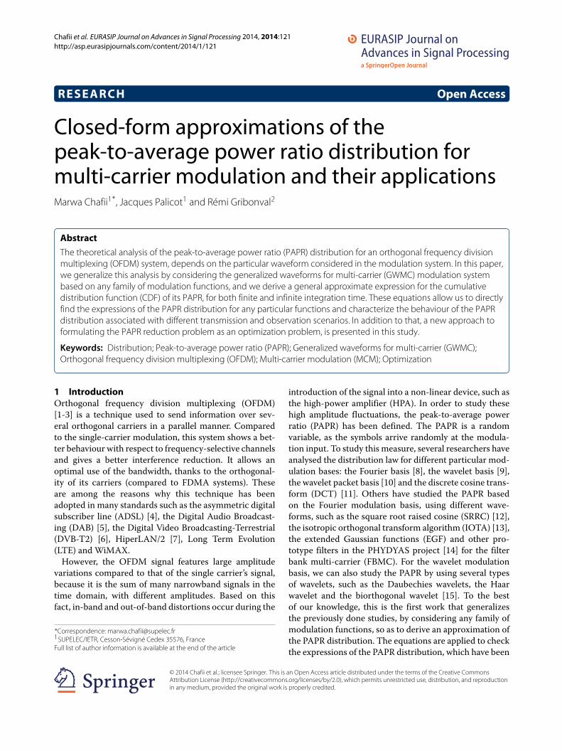
beyond the PAPRc,sup (see Figure 2). We can also mention

that the bound goes to infinity when the number of carri-

ersM goes to infinity, the CCDF is then equal to 1 for any

sufficiently small γ (see Figure 2).

In what follows, we give an approximation of the CDF

of the PAPR for γ sufficiently small compared with

PAPRc,sup. We leave to further work a mathematical quan-

tification of how small γ should be. For finite N , the

experiments show a good fit with our prediction.



Figure 2 PAPR distribution beyond its supremum.

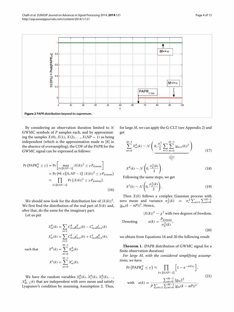
By considering an observation duration limited to N

GWMC symbols of P samples each, and by approximat-

ing the samples X(0), X(1), X(2), . . ., X(NP − 1) as being

independent (which is the approximation made in [8] in

the absence of oversampling), the CDF of the PAPR for the

GWMC signal can be expressed as follows:

Pr(

PAPRNd ≤ γ

)

= Pr

[

maxk∈[[0,NP−1]]

|X(k)|2 ≤ γPd,mean

]

= Pr(

∀k ∈[[ 0,NP − 1]] |X(k)|2 ≤ γPd,mean

)

≈∏

k∈[[0,NP−1]]

Pr(

|X(k)|2 ≤ γPd,mean

)

.

(16)

We should now look for the distribution law of |X(k)|2.

We first find the distribution of the real part of X(k) and,

after that, do the same for the imaginary part.

Let us put

XRm(k) =

∑

n∈Z

CRm,ng

Rm,n(k) − CI

m,ngIm,n(k)

XIm(k) =

∑

n∈Z

CRm,ng

Im,n(k) + CI

m,ngRm,n(k),

such that XR(k) =

M−1∑

m=0

XRm(k)

XI(k) =

M−1∑

m=0

XIm(k).

We have the random variables XR0 (k), XR

1 (k), XR2 (k), . . .,

XRM−1(k) that are independent with zero mean and satisfy

Lyapunov’s condition by assuming Assumption 2. Thus,

for largeM, we can apply the G-CLT (see Appendix 2) and

get

M−1∑

m=0

XRm(k) ∼ N

(

0,σ 2c

2

∑

n∈Z

M−1∑

m=0

|gm,n(k)|2

︸︷︷︸

σ2X (k)

2

)

(17)

XR(k) ∼ N

(

0,σ 2X(k)

2

)

. (18)

Following the same steps, we get

XI(k) ∼ N

(

0,σ 2X(k)

2

)

. (19)

Then X(k) follows a complex Gaussian process with

zero mean and variance σ 2X(k) = σ 2

c

∑

n∈Z

∑M−1m=0

|gm(k − nP)|2. Hence,

|X(k)|2 ∼ χ2 with two degrees of freedom.

Denoting x(k) =Pd,mean

σ 2X(k)

,

(20)

we obtain from Equations 16 and 20 the following result:

Theorem 1. (PAPR distribution of GWMC signal for a

finite observation duration)

For large M, with the considered simplifying assump-

tions, we have

Pr(

PAPRNd ≤ γ

)

≈∏

k∈ [[0,NP−1]]

[

1 − e−x(k)γ]

,

with x(k) =

∑M−1m=0 ‖gm‖2

P∑

n∈Z

∑M−1m=0 |gm(k − nP)|2

.

(21)



Note that the approximate distribution of the PAPR

depends not only on the family of modulation functions

(gm)m∈ [[0,M−1]] but also on the number of carriersM used.

In addition, it depends on the parameter N , the num-

ber of GWMC symbols observed. Taking into account the

simplifying assumption of our derivations, we can easily

study the PAPR performance of any multi-carrier mod-

ulation (MCM) system. The approximate expression of

the CDF of the PAPR will be compared to the empirical

CDF featured in Section 4.1. In Section 3.3, we deduce

the behaviour of the PAPR distribution for an infinite

observation period.

3.3 PAPR distribution for an infinite observation period

By considering an infinite number of GWMC symbols

observed, we can define the PAPR as being

Pr(

PAPR∞d ≤ γ

)

= Pr

[maxk∈N |X(k)|2

Pd,mean≤ γ

]

. (22)

To get the PAPR distribution in this case, we can let N

go to infinity in Equation 21; then, we obtain the following

formula:

Corollary 1. (PAPR distribution of GWMC signal for

an infinite observation duration)

For large M, with the considered simplifying assumptions,

we have

Pr(PAPR∞d ≤ γ ) = 0. (23)

In fact, we have

Pr(PAPR∞d ≤ γ ) =

∏

k∈N

[

1 − e−x(k)γ]

,

with x(k) =

∑M−1m=0 ‖gm‖2

P∑

n∈Z

∑M−1m=0 |gm(k − nP)|2

.

(24)

And we have

M−1∑

m=0

‖gm‖2 =

M−1∑

m=0

∑

n∈Z

P−1∑

k=0

|gm(k − nP)|2,

then A2MP <

M−1∑

m=0

‖gm‖2 < B2MP,

(25)

and1

B2MP<

1

M∑

n∈Z

∑M−1m=0 |gm,n(k)|2

<1

A2MP.

(26)

From Equations 25 and 26, we get

A2

B2< x(k) <

B2

A2, (27)

hence

(

1 − e−x(k)γ)

< 1 − e−

B2A2

γ< 1. (28)

Thus, for an infinite observation duration, and for γ

sufficiently small compared with PAPRc,sup, we have

Pr(PAPR∞d ≤ γ ) = 0. (29)

The CCDF is then equal to 1 for any γ (see Figure 3).

Equation 29 can be interpreted by the fact that we can-

not control the PAPR for an infinite number of GWMC

symbols, because we will inevitably have some GWMC

symbols with large peaks. Thus, for M ≥ 8 and γ suf-

ficiently small compared with PAPRc,sup and an infinite

observation duration, there is no family of modulation

functions (gm)m∈ [[0,M−1]] that can avoid the large peaks.

Based on this fact, we expect to optimize the PAPR

within a finite number of GWMC symbols. As the num-

ber of GWMC symbols decreases, PAPR optimization

gets better.

4 ApplicationsThe approximation of the PAPR distribution law for any

modulation system provides a valuable contribution to the

study of the PAPR problem in the case of MCM systems.

In particular, it allows us a fast computation of the PAPR

distribution for any family of modulation functions that

satisfies our conditions. Based on developed equations,

we are able to characterize the behaviour of the PAPR

distribution for different transmission and observation

scenarios and for any interval of γ . In addition to that, we

show how the PAPR reduction problem can be formulated

as an optimization problem. We give more details in the

following sections.

4.1 Simple computation of the PAPR for any family of

modulation functions

We know that the PAPR is a random variable, that is why

the derivation of its distribution law may be complex.

Especially if you have to repeat the derivation each time

the family of modulation functions changes. Equation 21

is a closed form approximation, so it allows us to directly

find an approximate CDF of the PAPR without complex

operations. To illustrate this, we consider the following

examples.

4.1.1 Conventional OFDM

Wewant to check the expression derived by VanNee in [8]

for the conventional OFDM for the discrete case. Then, let

us consider the following:



Figure 3 CCDF of the PAPR for an infinite observation duration.

• The Fourier basis is used for the modulation, with a

rectangular waveform:

gm(k) = ej2πmk

P �[0,P](k)

with �[0,P](k) =

{

1 if 0 ≤ k ≤ P

0 else.

• The observation is limited to one OFDM symbol, and

the number of samples considered isM then P = M.

The expression of the GWMC signal in Equation 1

becomes X(k) =∑

n∈Z

∑M−1m=0 Cm,ne

j2πm(k−nP)P �[0,P](k − nP).

We apply Equation 21 of the PAPR distribution with

N = 1. We then get

x(k) =MP

P∑

n∈Z

∑M−1m=0 |e

j2πm(k−nP)P �[0,P](k − nP)|2

= 1,

and then

Pr(

PAPR1d ≤ γ

)

=[

1 − e−γ]M

. (30)

It is similar to the expression derived by Van Nee for the

discrete case.

4.1.2 FBMC systems

We consider the OFDM/OQAM as being an example of

the FBMC system, and we check the expression derived by

Skrzypczak [22]. Then, let us consider the following:

• The modulation functions are

gm(k − nP) = hOQAM(k − nP)

ej2πmM (k − D/2)ejθm,n ,

then |gm(k − nP)|2 = h2OQAM(k − nP),

where hOQAM is the prototype filter (IOTA, SRRC,

PHYDYAS...).• The observation is limited to one block of symbols,

and the number of samples considered in this block is

M, then P = M.

• ‖gm‖2 = 1.

The expression of the GWMC signal in

Equation 1 becomes X(k) =∑

n∈Z

∑M−1m=0 Cm,nhOQAM

(k − nP)ej2πmM (k − D/2)ejθm,n .

We apply Eq. (21) of the discrete-time PAPR for a finite

observation duration with N = 1. Then, we get

x(k) =1

M∑

n∈Z h2OQAM(k − nP)

and then

Pr(PAPR1d ≤ γ ) =

M−1∏

k=0

[

1 − e

−γ

M∑

n∈Z h2OQAM

(k−nP)

]

.

(31)

This result is similar to the one obtained by Skrzypczak.

4.1.3 NOFDM systems

The family of modulation functions used in NOFDM sys-

tems is not orthogonal, but it forms an incomplete Riesz

basis. The choice of the non-orthogonal pulses is flexi-

ble and can be adapted to the knowledge of the channel;

therefore, NOFDM systems have a better bandwidth effi-

ciency than OFDM systems and tends to be more robust

against frequency-selective fading [16]. To provide an

example of an NOFDM system, we consider Hamming

window w(t), which is a non-orthogonal pulse. Thus, the

waveform of the modulation is expressed as

gm(t) = ej2πmtT w(t),

w(t) =

⎧

⎪⎨

⎪⎩

0.54 − 0.46 cos

(

2πt

T

)

if 0 ≤ t ≤ T

0 else

Figure 4 shows the theoretical CCDF of the PAPR

based on Equation 1 with P = M and N = 1 and



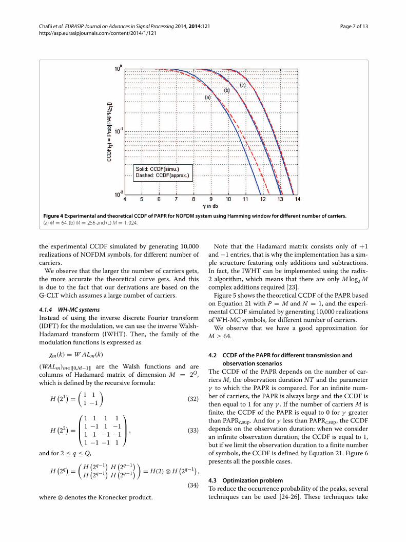
Figure 4 Experimental and theoretical CCDF of PAPR for NOFDM system using Hamming window for different number of carriers.

(a)M = 64, (b)M = 256 and (c)M = 1, 024.

the experimental CCDF simulated by generating 10,000

realizations of NOFDM symbols, for different number of

carriers.

We observe that the larger the number of carriers gets,

the more accurate the theoretical curve gets. And this

is due to the fact that our derivations are based on the

G-CLT which assumes a large number of carriers.

4.1.4 WH-MC systems

Instead of using the inverse discrete Fourier transform

(IDFT) for the modulation, we can use the inverse Walsh-

Hadamard transform (IWHT). Then, the family of the

modulation functions is expressed as

gm(k) = W ALm(k)

(WALm)m∈ [[0,M−1]] are the Walsh functions and are

columns of Hadamard matrix of dimension M = 2Q,

which is defined by the recursive formula:

H(

21)

=

(

1 1

1 −1

)

(32)

H(

22)

=

⎛

⎜⎜⎝

1 1 1 1

1 −1 1 −1

1 1 −1 −1

1 −1 −1 1

⎞

⎟⎟⎠, (33)

and for 2 ≤ q ≤ Q,

H(

2q)

=

(

H(

2q−1)

H(

2q−1)

H(

2q−1)

H(

2q−1)

)

= H(2) ⊗ H(

2q−1)

,

(34)

where ⊗ denotes the Kronecker product.

Note that the Hadamard matrix consists only of +1

and −1 entries, that is why the implementation has a sim-

ple structure featuring only additions and subtractions.

In fact, the IWHT can be implemented using the radix-

2 algorithm, which means that there are only M log2M

complex additions required [23].

Figure 5 shows the theoretical CCDF of the PAPR based

on Equation 21 with P = M and N = 1, and the experi-

mental CCDF simulated by generating 10,000 realizations

of WH-MC symbols, for different number of carriers.

We observe that we have a good approximation for

M ≥ 64.

4.2 CCDF of the PAPR for different transmission and

observation scenarios

The CCDF of the PAPR depends on the number of car-

riers M, the observation duration NT and the parameter

γ to which the PAPR is compared. For an infinite num-

ber of carriers, the PAPR is always large and the CCDF is

then equal to 1 for any γ . If the number of carriers M is

finite, the CCDF of the PAPR is equal to 0 for γ greater

than PAPRc,sup. And for γ less than PAPRc,sup, the CCDF

depends on the observation duration: when we consider

an infinite observation duration, the CCDF is equal to 1,

but if we limit the observation duration to a finite number

of symbols, the CCDF is defined by Equation 21. Figure 6

presents all the possible cases.

4.3 Optimization problem

To reduce the occurrence probability of the peaks, several

techniques can be used [24-26]. These techniques take



Figure 5 Experimental and theoretical CCDF values of PAPR for a WH-MC system for different number of carriers. (a)M = 64, (b)M = 256

and (c)M = 1, 024.

place before and after the modulation. But as we can see

in Equation 21, the distribution of the PAPR depends on

the family of modulation functions used in the system.

Thus, we can act also on the modulation system to reduce

the PAPR. In fact, to confirm this idea, we can com-

pare the PAPR performance of the OFDM/OQAM [13]

to that of the wavelet OFDM [27]. The first variant uses

the same modulation basis as the conventional OFDM

(Fourier basis) and does not show any improvement on

the PAPR’s performance [22], unlike the second that uses

the wavelet basis and shows an improvement of up to

2 dB [28].

Let us model the PAPR’s optimization problem. It con-

sists in finding the optimal functions gm that maximize the

CDF of the PAPR in Equation 21. By trying to do that, we

notice that we should do the optimization at some par-

ticular points of the functions gm (the sampling points),

while these points are not chosen in a particular way.

Figure 6 PAPR distribution for different transmission and observation scenarios.



To adjust the optimization problem, we approximate the

denominator of x(k). Let us put

Sp = ln(

Pr(

PAPRNd ≤ γ

))

=

NP−1∑

k=0

ln

⎛

⎝1 − e−

∑M−1m=0 ‖gm‖2

P∑

n∈Z∑M−1

m=0 |gm,n(k TP )|2γ

⎞

⎠ ,

and we put

h(x) = ln

⎛

⎝1 − e−

∑M−1m=0 ‖gm‖2

P∑

n∈Z∑M−1

m=0 |gm,n(x)|2γ

⎞

⎠ ,

We have h : [0,NT]→ R is piecewise continuous over

[0,NT], and we have

NT

NPSp =

NT

NP

NP−1∑

k=0

h

(

kNT

NP

)

is a Riemann sum, then

T

PSp ≈

∫ NT

0h(x) dx

⇒1

PSp ≈

1

T

∫ NT

0h(x) dx

⇒ Sp =P

T

∫ NT

0h(x) dx + o(P)

⇒ Pr(

PAPRNd ≤ γ

)

= ePT

∫ NT0 h(x) dx + o(P).

Maximizing Pr(

PAPRNd ≤ γ

)

is equivalent to maxi-

mizing∫ NT0 h(x) dx, and it is equivalent to maximizing

∫ T0 h(x) dx since h is a periodic function of T . Then,

the quantity that we should maximize over the functions

(gm)m∈ [[0,M−1]] is

∫ T

0ln

⎛

⎝1 − e−

∑M−1m=0 ‖gm‖2

P∑

n∈Z∑M−1

m=0 |gm,n(t)|2γ

⎞

⎠ dt. (35)

To express the optimization problem that can lead to

a new modulation system featuring an optimally reduced

PAPR, we have to express the constraints on the functions

(gm)m∈ [[0,M−1]]. Let us define the following constraints:

• C0 = {(gm)m∈ [[0,M−1]]/forM large

3

√∑M−1

m=0 E|∑

n∈Z CRm,ng

Rm,n(t) − CI

m,ngIm,n(t)|

3

√

σ 2c2

∑M−1m=0

∑

n∈Z |gm(t − nT)|2< ǫM ≪ 1,

3

√∑M−1

m=0 E|∑

n∈Z CRm,ng

Im,n(t) + CI

m,ngRm,n(t)|

3

√

σ 2c2

∑M−1m=0

∑

n∈Z |gm(t − nT)|2< ǫ

′

M ≪ 1}

C0 is the condition that we need to apply CLT. We

considered Assumption 2 because the expression of

C0 is not intuitive.• C1 =

{

(gm)m∈ [[0,M−1]]/for largeM maxm,t∑

n∈Z |gm(t − nT)| = B1 < +∞ andminm,t∑

n∈Z

|gm(t − nT)|2 = A2 > 0}

. C1 is the set of functions

that satisfy Assumption 2. C1 is stronger than C0.• C2 =

{

(gm)m∈ [[0,M−1]]/∀m ∈ [[ 0,M − 1]]∑

n∈Z

|gm,n(t)|2 =

∑

n∈Z |g0,n(t)|2}

. C2 is stronger than C0

and C1 but easy to manipulate.

These conditions define the choice of the functions

(gm)m∈ [[0,M−1]]. Figure 7 shows the inclusion relationship

between the different conditions.

Thus, the optimization problem can be expressed as

follows:

Optimization problem (i)

maximize(gm)m∈ [[0,M−1]]

∫ T0 ln

⎛

⎝1 − e−

∑M−1m=0 ‖gm‖2

P∑

n∈Z∑M−1

m=0 |gm,n(t)|2γ

⎞

⎠ dt,

subject to(

gm)

m∈ [[0,M−1]]∈ Ci.

The present study proposes to act on the modulation

system to reduce the PAPR. Looking for the optimal fam-

ily of modulation functions is a new approach to deal

with the PAPR problem. Its advantage is that we can use,

at the same time, one of the previous PAPR reduction

techniques to get an even smaller PAPR.

5 ConclusionsIn this paper, we make several derivations to achieve the

more general CDF approximation of the PAPR in the

sense that transmitted symbols can be carried by any

family of functions. First, we define the GWMC system

and derive a general approximation of its PAPR distri-

bution for both finite and infinite integration time. We

conclude that the PAPR distribution depends on the fam-

ily of functions used in the modulation, but for an infinite

observation duration, large peaks cannot be avoided, even

if we change the family of modulation functions. To show

the importance of developed expressions, we illustrate

their applications: the simple computation of the PAPR

distribution of any modulation system, the characteriza-

tion of the CCDF of the PAPR for different transmission

and observation scenarios, as well as the modelling of the

PAPR reduction problem as a constrained optimization

problem.

The remaining difficulty is to solve the optimization

problem. This needs to be addressed by future stud-

ies. Other constraints should be added, which take into

account the required performance of the system, such as

the bit error rate (BER) and the implementation complex-

ity. The solution of this constrained optimization problem



Figure 7 Relationship between the optimization problem’s constraints.

can lead to a new system of multi-carrier modulation

featuring an optimal performance.

Appendix 1Berry-Esseen theorem

In probability theory, the CLT states that, under cer-

tain circumstances, the probability distribution of the

scaled mean of a random sample converges to a nor-

mal distribution as the sample size increases to infinity.

Under stronger assumptions, the Berry-Esseen theorem,

or Berry-Esseen inequality, specifies the rate at which this

convergence takes place by giving a bound on themaximal

error of approximation between the normal distribution

and the true distribution of the scaled sample mean. In the

case of independent samples, the convergence rate is√

1M .

In general, we have a good approximation for the Gaussian

curve forM > 8.

In our case, we perform simulations by considering the

number of carriers to be equal toM = 64 > 8. Under this

assumption, the following Lyapunov’s condition:

limM→+∞

3

√∑M−1

m=0 E|∑

n∈ZCRm,ng

Rm,n(t)−CI

m,ngIm,n(t)|

3

√

σ 2c2

∑M−1m=0

∑

n∈Z |gm(t − nT)|2= 0

and limM→+∞

3

√∑M−1

m=0 E|∑

n∈ZCRm,ng

Im,n(t)+CI

m,ngRm,n(t)|

3

√

σ 2c2

∑M−1m=0

∑

n∈Z |gm(t − nT)|2= 0

becomes

3

√∑M−1

m=0 E|∑

n∈Z CRm,ng

Rm,n(t) − CI

m,ngIm,n(t)|

3

√

σ 2c2

∑M−1m=0

∑

n∈Z |gm(t − nT)|2< ǫM ≪ 1

and

3

√∑M−1

m=0 E|∑

n∈Z CRm,ng

Im,n(t) + CI

m,ngRm,n(t)|

3

√

σ 2c2

∑M−1m=0

∑


′

M ≪ 1.

Appendix 2Distribution of XR(t)

A. Lyapunov CLT

Let us suppose that X1,X2, . . . is a sequence of indepen-dent random variables, each with finite expected valueμm

and a variance σ 2m. Let us define

s2M =

M∑

m=1

σ 2m,

and the third-order centred moments

r3M =

M∑

m=1

E(

|Xm − μm|3)

.

Lyapunov’s condition is

limM→+∞

rM

sM= 0.

Let us put SM = X1 + X2 + · · · + XM. The expectation

of SM ismM =∑M

m=1 μm and its standard deviation is sM.

If Lyapunov’s condition is satisfied, then SM−mMsM

converges

in distribution to a standard normal random variable, asM goes to infinity:

SM − mM

sM∼ N (0, 1).

B. Lyapunov’s condition for GWMC

Property 1. (Lyapunov’s condition)

When Assumption 2 holds, there are constants Ai > 0 and

B2 < +∞ such that for all m, t

0 < A1 ≤∑

n∈Z

|gm(t − nT)| ≤ B1 < +∞ (36)

and 0 < A2 ≤∑

n∈Z

|gm(t − nT)|2 ≤ B2 < +∞. (37)

Moreover,

3

√∑M−1

m=0 E|∑

n∈ZCRm,ng

Rm,n(t)−CI

m,ngIm,n(t)|

3

√

σ 2c2

∑M−1m=0

∑

n∈Z |gm(t − nT)|2<ǫM ≪1, (38)



and

3

√∑M−1

m=0 E|∑

n∈Z CRm,ng

Im,n(t) + CI

m,ngRm,n(t)|

3

√

σ 2c2

∑M−1m=0

∑


′

M ≪ 1.

(39)

Proof. Let maxm,t∑

n∈Z |gm(t − nT)| = B1 < +∞ and

minm,t∑

n∈Z |gm(t − nT)|2 = A2 > 0. We have

∑

n∈Z

|gm(t − nT)| ≤ B1 < +∞ (40)

⇒∑

n∈Z

|gm(t − nT)|2 ≤ B21 < +∞

⇒ maxm,t

∑

n∈Z

|gm(t − nT)|2 = B2 ≤ B21 < +∞, (41)

and we have

∑

n∈Z

|gm(t − nT)|2 ≥ A2 > 0 (42)

⇒∑

n∈Z

|gm(t − nT)| ≥

√∑

n∈Z

|gm(t − nT)|2 ≥√

A2

⇒ minm,t

∑

n∈Z

|gm(t − nT)| = A1 ≥√

A2 > 0. (43)

We want to prove the validity of Lyapunov’condition.

We have

1√

B2Mσ 2c2

≤1

√

σ 2c2

∑M−1m=0

∑

n∈Z |gm(t − nT)|2≤

1√

A2Mσ 2c2

,

(44)

and we have

|CRm,ng

Rm,n(t)| ≤ max

m,nCRm,n

︸︷︷︸

CR

|gRm,n(t)| and

|CIm,ng

Im,n(t)| ≤ max

m,nCIm,n

︸︷︷︸

CI

|gIm,n(t)|

∑

n∈Z

|CRm,ng

Rm,n(t)| ≤ CRB1 and

∑

n∈Z

|CIm,ng

Im,n(t)| ≤ CIB1

then |∑

n∈Z

CRm,ng

Rm,n(t) − CI

m,ngIm,n(t)|

≤ |∑

n∈Z

CRm,ng

Rm,n(t)| − |

∑

n∈Z

CIm,ng

Im,n(t)|

≤∑

n∈Z

|CRm,ng

Rm,n(t)| −

∑

n∈Z

|CIm,ng

Im,n(t)|

≤ CRB1 + CIB1

and so

|∑

n∈Z

CRm,ng

Rm,n(t) − CI

m,ngIm,n(t)|

3 ≤ (CRB1 + CIB1)3

thus E

(

|∑

n∈Z

CRm,ng

Rm,n(t) − CI

m,ngIm,n(t)|

3

)

≤ (CRB1 + CIB1)3 .

(45)

From Equations 44 and 45, we have

3

√∑M−1

m=0 E|∑

n∈Z CRm,ng

Rm,n(t) − CI

m,ngIm,n(t)|

3

√

σ 2c2

∑M−1m=0

∑

n∈Z |gm(t − nT)|2

≤

3√

M(CRB1 + CIB1)3√

A2Mσ 2c2

. (46)

For largeM, we have

3

√∑M−1

m=0 E|∑

n∈Z CRm,ng

Rm,n(t) − CI

m,ngIm,n(t)|

3

√

σ 2c2

∑M−1m=0

∑

n∈Z |gm(t − nT)|2

< ǫM = O(

M−1/6)

≪ 1.

We can prove the second part of Lyapunov’s condition

by proceeding similarly. Assumption 2 is then a sufficient

condition of Lyapunov’s condition.

C. Application of Lyapunov CLT

Let us put XRm(t) =

∑

n∈Z CRm,ng

Rm,n(t) − CI

m,ngIm,n(t) such

that XR(t) =∑M−1

m=0 XRm(t). In our case, we have XR

0 (t),

XR1 (t), XR

2 (t), . . ., XRM−1(t) is a sequence of independent

random variables (Assumption 1). And we have

• From Equation 4, ∀m ∈[[ 0,M − 1]] E(XRm(t)) = 0.

• Var(XRm(t)) =

∑

n∈Z

σ 2c2 |gm,n(t)|

2.



In fact,

Var(

XRm(t)

)

= E(

XRm(t)2

)

= E

⎛

⎝

∑

n,p∈Z

[

CRm,ng

Rm,n(t) − CI

m,ngIm,n(t)

]

×

[

CRm,pg

Rm,p(t) − CI

m,pgIm,p(t)

]

⎞

⎠

= E

⎛

⎝

∑

n,p∈Z

[

CRm,nC

Rm,pg

Rm,n(t)g

Rm,p(t)

− CRm,nC

Im,pg

Rm,n(t)g

Im,p(t)

− CIm,nC

Rm,pg

Im,n(t)g

Rm,p(t)

+ CIm,nC

Im,pg

Im,n(t)g

Im,p(t)

]

⎞

⎠

=∑

n∈Z

σ 2c

2

[(

gRm,n(t))2

+(

gIm,n(t))2]

(Eq. 2, 3, 4, 5)

=∑

n∈Z

σ 2c

2|gm,n(t)|

2.

• rM =3

√∑M−1

m=0 E|∑

n∈Z CRm,ng

Rm,n(t) − CI

m,ngIm,n(t)|

3.

• sM =

√∑M−1

m=0 Var(

XRm

)

=

√

σ 2c2

∑M−1m=0

∑

n∈Z |gm,n(t)|2.

From Assumption 2, we have limM→+∞rMsM

= 0.

Lyapunov’s condition is then satisfied. By means of

Lyapunov’s CLT, we get for largeM

∑M−1m=0 X

Rm(t)

σ 2c2

∑

n∈Z

∑M−1m=0 |gm,n(t)|2

∼ N (0, 1)

M−1∑

m=0

XRm(t) ∼ N

(

0,σ 2c

2

∑

n∈Z

M−1∑

m=0

|gm,n(t)|2

)

.

Appendix 3Average power’s expression

The average power is calculated as follows:

Pc,mean = limt0→+∞

1

2t0

∫ t0

−t0

E(

|X(t)|2)

dt

= limt0→+∞

1

2t0

∫ t0

−t0

E

⎛

⎝

M−1∑

m,m′=0

∑

n,n′∈Z

Cm,nC∗m′ ,n′gm,n(t)g

∗m′ ,n′(t)

⎞

⎠dt

Assumption 1= lim

t0→+∞

1

2t0

∫ t0

−t0

M−1∑

m=0

∑

n∈Z

σ 2c |gm,n(t)|

2 dt

= σ 2c limt0→+∞

1

2t0

M−1∑

m=0

∫ t0

−t0

∑

n∈Z

|gm,n(t)|2 dt.

Let us put t0 = KT2 ,K ∈ N

Pc,mean =σ 2c

Tlim

K→+∞

1

K

M−1∑

m=0

∫ KT2

− KT2

∑

n∈Z

|gm,n(t)|2 dt.

We notice that t �→∑

n∈Z

∑M−1m=0 |gm(t − nT)|2 is

periodic with a period T , so

Pc,mean =σ 2c

T

M−1∑

m=0

∫ T2

− T2

∑

n∈Z

|gm(t − nT)|2 dt

(by periodicity)=

σ 2c

T

M−1∑

m=0

∑

n∈Z

∫ nT+ T2

nT− T2

|gm(t − nT)|2 dt

=σ 2c

T

M−1∑

m=0

∫ +∞

−∞

|gm(t)|2 dt

Pc,mean =σ 2c

T

M−1∑

m=0

‖gm‖2.

Appendix 4Upper bound of the PAPR [29]

Let M be a finite number of carriers and (gm)m∈[[0,M−1]]

a family of modulation functions that satisfies

Ai = minm,t∑

n∈Z |gm(t − nT)|i > 0 and Bi = maxm,t∑

n∈Z |gm(t − nT)|i < +∞ for i ∈ {1, 2}. For any obser-

vation duration I and any input symbols, we have

PAPRc(I) =maxt∈I |X(t)|2

Pc,mean. (47)

We have

maxt∈I

|X(t)| = maxt∈I

|∑

n∈Z

M−1∑

m=0

Cm,ngm(t − nT)|

≤ maxt∈I

M−1∑

m=0

|∑

n∈Z

Cm,ngm(t − nT)|

≤ maxm,n

M−1∑

m=0

|Cm,n|∑

n∈Z

|gm(t − nT)|

≤ Mmaxm,n

|Cm,n|B1,

(48)

and we have

Pc,mean =σ 2c

T

M−1∑

m=0

∫ T2

− T2

∑

n∈Z

|gm(t − nT)|2 dt, (49)

hence MA2σ2C ≤ Pc,mean ≤ MB2σ

2C . (50)

Thus,

PAPRc(I) ≤maxm,n |Cm,n|

2B21

σ 2CA2

M. (51)



Abbreviations

ADSL: asymmetric digital subscriber line; BER: bit error rate; BFDM:

biorthogonal frequency division multiplexing; CDF: cumulative distribution

function; CCDF: complementary cumulative distribution function; CLT: central

limit theorem; DAB: Digital Audio Broadcasting; DCT: discrete cosine

transform; DVB-H: Digital Video Broadcasting-Handheld; DVB-T: Digital Video

Broadcasting-Terrestrial; EGF: extended Gaussien function; FSK: frequency Shift

Keying; GWMC: generalized waveforms for multi-carrier; GCLT: generalized

central limit theorem; HiperLAN/2: high performance radio LAN; HPA: high-

power amplifier; IOTA: isotropic orthogonal transform algorithm; LTE: Long

Term Evolution; NOFDM: non-orthogonal frequency division multiplexing;

OFDM: orthogonal frequency division multiplexing; OQAM: offset quadrature

amplitude modulation; PAPR: peak-to-average power ratio; PSK: phase shift

keying; QAM: quadrature amplitude modulation; QPSK: quadrature phase shift

keying; SRRC: square root raised cosine; WH-HT: Walsh-Hadamard multi-carrier.

Competing interests

The authors declare that they have no competing interests.

Acknowledgements

This work has received a French state support granted to the CominLabs

excellence laboratory and managed by the National Research Agency in the

‘Investing for the Future’ program under reference no. ANR-10-LABX-07-01.

The authors would also like to thank the ‘Région Bretagne’, France for

supporting this work.

Author details1SUPELEC/IETR, Cesson-Sévigné Cedex 35576, France. 2 Inria, Bretagne

Atlantique, Campus de Beaulieu, Rennes Cedex 35042, France.

Received: 1 December 2013 Accepted: 17 July 2014

Published: 30 July 2014

References

1. RW Chang, Synthesis of band-limited orthogonal signals for multichannel

data transmission. Bell Sys. Tech. J. 45, 1775–1796 (1966)

2. S Weinstein, P Ebert, Data transmission by frequency-division

multiplexing using the discrete Fourier transform. Commun. Technol. IEEE

Trans. 19(5), 628–634 (1971)

3. R Lassalle, M Alard, Principles of modulation and channel coding for digital

broadcasting for mobile receivers. EBU Tech. Rev. 224, 168–190 (1987)

4. ETSI TS 101 388 V1. 3.1 (2002–05), Asymmetric Digital Subscriber Line

(ADSL)-European specific requirements (2002)

5. Digital Audio Broadcasting (DAB); DAB to mobile, portable and fixed

Receivers, Tech. Rep. ETSI ETS 300 401 (1995)

6. ETSI EN 302 755 v1. 2.1 (2010-10) Digital Video Broadcasting (DVB), Frame

structure channel coding and modulation for a second generation digital

terrestrial television broadcasting system (DVB-T2)

7. ETSI TS 101 475 V1. 3.1 (2001-12), Broadband radio access networks

(BRAN); HIPERLAN type 2; physical (PHY) layer (2001)

8. R Van Nee, R Prasad, OFDM for Wireless Multimedia Communications.

(Artech House Inc., Norwood, 2000)

9. M Hoch, S Heinrichs, JB Huber, Peak-to-average power ratio and its

reduction in wavelet-OFDM, in International OFDMWorkshop (Hamburg,

Germany, 2011), pp. 56–60

10. M Gautier, C Lereau, M Arndt, J Lienard, PAPR analysis in wavelet packet

modulation, in 3rd International SymposiumOn Communications, Control

and Signal Processing, 2008. ISCCSP 2008 (IEEE St Julians, 2008), pp. 799–803

11. L Patidar, A Parikh, BER Comparison of DCT-based OFDM and FFT-based

OFDM using BPSK modulation over AWGN and multipath Rayleigh fading

channel. Int. J. Comput. Appl. 31(10), 38–41 (2011). New York, USA

12. P Chevillat, G UngerBoeck, Optimum FIR transmitter and receiver filters

for data transmission over band-limited channels. Commun. IEEE Trans.

30(8), 1909–1915 (1982)

13. B Le Floch, M Alard, C Berrou, Coded orthogonal frequency division

multiplex. Proc. IEEE. 83(6), 24–182 (1995)

14. A Viholainen, M Bellanger, M Huchard, Prototype filter and structure

optimization. PHYDYAS project, January 2009

15. H Zhang, D Yuan, M Pätzold, Novel study on PAPRs reduction in

wavelet-based multicarrier modulation systems. Digital Signal Process.

17(1), 272–279 (2007)

16. W Kozek, AF Molisch, Nonorthogonal pulseshapes for multicarrier

communications in doubly dispersive channels. Selected Areas Commun.

IEEE J. 16(8), 1579–1589 (1998)

17. H Bogucka, AM Wyglinski, S Pagadarai, A Kliks, Spectrally agile multicarrier

waveforms for opportunistic wireless access. Commun. Mag. IEEE.

49(6), 108–115 (2011)

18. A Aboltins, Comparison of orthogonal transforms for OFDM

communication system. Electronics and Electrical Engineering.

111(5), 77–80 (2011)

19. M Chafii, J Palicot, R Gribonval, Closed-Form Approximations of the PAPR

Distribution for Multi-Carrier Modulation Systems. (Lisbon, Eusipco, 2014)

20. B Knaeble, Variations on the projective central limit theorem. PhD thesis,

University of Utah, 2010

21. C Siclet, Application de la théorie des bancs de filtres à l’analyse et à la

conception de modulations multiporteuses orthogonales et

biorthogonales. PhD thesis, Rennes 1 University, France, 2002

22. A Skrzypczak, Contribution à l’étude des modulations multiporteuses

OFDM/OQAM et OFDM suréchantillonnées. PhD thesis, Rennes 1

University, France, 2007

23. BG Evans, G Bi, Hardware structure for Walsh-Hadamard transforms.

Electron. Lett. 34(21), 2005–2006 (1998)

24. L Wang, J Liu, PAPR reduction of OFDM signals by PTS with grouping and

recursive phase weighting methods. Broadcast. IEEE Trans. 57(2), 299–306

(2011)

25. C-P Li, S-H Wang, C-L Wang, Novel low-complexity SLM schemes for PAPR

reduction in ofdm systems. Signal Process. IEEE Trans. 58(5), 2916–2921

(2010)

26. D Guel, J Palicot, Transformation des techniques “ajout de signal” en

techniques “tone reservation” pour la réduction du PAPR des signaux OFDM.

(GRETSI, Dijon, 2009)

27. Rishabh K, K Nachiket, N Piyush. EE678 Wavelet Application Assignment,

Wavelet OFDM

28. MHM Nerma, NS Kamel, V Jeoti, NA Baykara, NE Mastorakis, BER

performance analysis of OFDM system based on dual-tree complex wavelet

transform in AWGN channel. (Istanbul, Turkey, 2009)

29. M Chafii, J Palicot, R Gribonval, A PAPR upper bound of Generalized

Waveforms for Multi-Carrier modulation systems, in ISCCSP, 6th

International Symposium on Communications, Control and Signal

Processing (Athens, 2014)

doi:10.1186/1687-6180-2014-121Cite this article as: Chafii et al.: Closed-form approximations of the peak-to-average power ratio distribution for multi-carrier modulation and theirapplications. EURASIP Journal on Advances in Signal Processing 2014 2014:121.

Submit your manuscript to a journal and benefi t from:

7 Convenient online submission

7 Rigorous peer review

7 Immediate publication on acceptance

7 Open access: articles freely available online

7 High visibility within the fi eld

7 Retaining the copyright to your article

Submit your next manuscript at 7 springeropen.com

Documents

Closed-form approximations of the peak-to-average power