Close Range Photogrammetry - tutissolutions.com · Society for Photogrammetry, Remote Sensing and Geoinformation) DGZfP Deutsche Gesellschaft für Zerstörungsfreie Prüfung (German

Close Range Photogrammetry

Close RangePhotogrammetry

Principles, techniques and applications

T Luhmann, S Robson, S Kyle and I Harley

Whittles Publishing

Published byWhittles Publishing,

Dunbeath Mains Cottages,Dunbeath,

Caithness KW6 6EY,Scotland, UK

www.whittlespublishing.com

© 2006 T Luhmann, S Robson, S Kyle and I Harley

ISBN 1-870325-50-8

All rights reserved.No part of this publication may be reproduced,

stored in a retrieval system, or transmitted,in any form or by any means, electronic,

mechanical, recording or otherwisewithout prior permission of the publishers.

Typeset by Compuscript Ltd, Shannon, Ireland

Printed by (information to be supplied)

Contents

Abbreviations .........................................................................................................................x

Image sources ......................................................................................................................xii

1 Introduction......................................................................................................................1

1.1 Overview ......................................................................................................................11.2 Fundamental methods...................................................................................................2

1.2.1 The photogrammetric process ..........................................................................21.2.2 Aspects of photogrammetry .............................................................................31.2.3 Image forming model .......................................................................................61.2.4 Photogrammetric systems.................................................................................81.2.5 Photogrammetric products..............................................................................11

1.3 Applications................................................................................................................131.4 Historical development...............................................................................................15References and further reading ............................................................................................25

2 Mathematical fundamentals ....................................................................................31

2.1 Coordinate systems.....................................................................................................312.1.1 Image and camera coordinate systems ...........................................................312.1.2 Comparator coordinate system.......................................................................322.1.3 Model coordinate system................................................................................322.1.4 Object coordinate system ...............................................................................332.1.5 3D instrument coordinate system...................................................................33

2.2 Coordinate transformations ........................................................................................342.2.1 Plane transformations .....................................................................................342.2.2 Spatial transformations...................................................................................39

2.3 Adjustment techniques ...............................................................................................522.3.1 The problem....................................................................................................522.3.2 Least-squares method (Gauss-Markov linear model).....................................552.3.3 Measures of quality ........................................................................................592.3.4 Error detection in practice ..............................................................................672.3.5 Computational aspects....................................................................................70

2.4 Geometric elements ....................................................................................................722.4.1 Analytical geometry in the plane ...................................................................732.4.2 Analytical geometry in 3D space ...................................................................822.4.3 Surfaces ..........................................................................................................902.4.4 Compliance with design .................................................................................93

References ...........................................................................................................................94

3 Imaging technology .....................................................................................................97

3.1 Imaging concepts........................................................................................................973.1.1 Methods of image acquisition ........................................................................973.1.2 Imaging configurations...................................................................................98

3.2 Geometric fundamentals...........................................................................................1003.2.1 Image scale and accuracy .............................................................................1003.2.2 Optical imaging ............................................................................................1043.2.3 Interior orientation of a camera....................................................................1143.2.4 Resolution .....................................................................................................1293.2.5 Fundamentals of sampling theory ................................................................132

3.3 Imaging systems .......................................................................................................1353.3.1 Analogue imaging systems...........................................................................1353.3.2 Digital imaging systems ...............................................................................1473.3.3 Laser-based measuring systems....................................................................1763.3.4 Other imaging systems .................................................................................181

3.4 Targeting and illumination .......................................................................................1833.4.1 Object targeting ............................................................................................1833.4.2 Illumination techniques ................................................................................190

References .........................................................................................................................195

4 Analytical methods ....................................................................................................201

4.1 Overview ..................................................................................................................2014.2 Orientation methods .................................................................................................202

4.2.1 Exterior orientation.......................................................................................2024.2.2 Collinearity equations...................................................................................2044.2.3 Orientation of single images.........................................................................2064.2.4 Object position and orientation by inverse resection ...................................2144.2.5 Orientation of stereo image pairs .................................................................215

4.3 Bundle triangulation .................................................................................................2294.3.1 General remarks............................................................................................2294.3.2 Mathematical model .....................................................................................2344.3.3 Object coordinate system (definition of datum) ..........................................2444.3.4 Generation of approximate values................................................................2514.3.5 Quality measures and analysis of results......................................................2604.3.6 Strategies for bundle adjustment ..................................................................264

4.4 Object reconstruction ...............................................................................................2664.4.1 Single image processing ...............................................................................2664.4.2 Stereoscopic processing................................................................................2744.4.3 Multi-image processing ................................................................................283

4.5 Line photogrammetry ...............................................................................................2934.5.1 Space resection using parallel object lines...................................................2934.5.2 Collinearity equations for straight lines .......................................................2964.5.3 Relative orientation with straight lines.........................................................297

Contents

vi

4.5.4 3D similarity transformation with straight lines ..........................................2994.5.5 Bundle adjustment with straight lines ..........................................................3004.5.6 Bundle adjustment with geometric elements ...............................................301

4.6 Multi-media photogrammetry ..................................................................................3024.6.1 Light refraction at media interfaces .............................................................3024.6.2 Extended model of bundle triangulation ......................................................307

4.7 Panoramic photogrammetry .....................................................................................3094.7.1 Cylindrical panoramic imaging model .........................................................3094.7.2 Orientation of panoramic imagery ...............................................................3114.7.3 Epipolar geometry ........................................................................................3134.7.4 Spatial intersection .......................................................................................315

References ..........................................................................................................................315

5 Digital image processing..........................................................................................319

5.1 Fundamentals............................................................................................................3195.1.1 Image processing procedure .........................................................................3195.1.2 Pixel coordinate system................................................................................3205.1.3 Handling image data.....................................................................................322

5.2 Image preprocessing.................................................................................................3275.2.1 Point operations ............................................................................................3275.2.2 Filter operations ............................................................................................3335.2.3 Edge extraction .............................................................................................339

5.3 Geometric image transformation..............................................................................3505.3.1 Fundamentals of rectification.......................................................................3515.3.2 Grey value interpolation ...............................................................................3525.3.3 3D visualisation ............................................................................................354

5.4 Digital processing of single images .........................................................................3615.4.1 Approximate values ......................................................................................3615.4.2 Measurement of single point features ..........................................................3645.4.3 Contour following.........................................................................................376

5.5 Image matching and 3D object reconstruction ........................................................3785.5.1 Overview.......................................................................................................3785.5.2 Feature-based matching procedures .............................................................3805.5.3 Correspondence analysis based on epipolar geometry ................................3855.5.4 Area-based multi-image matching ...............................................................3885.5.5 Matching methods with object models.........................................................392

References .........................................................................................................................397

6 Photogrammetric measuring systems................................................................401

6.1 Comparators..............................................................................................................4016.1.1 Design principles ..........................................................................................4016.1.2 Analogue image comparators .......................................................................4026.1.3 Digital image comparators ...........................................................................402

Contents

vii

6.2 Single camera systems..............................................................................................4046.2.1 Camera with hand-held probing device........................................................4046.2.2 Probing system with integrated camera .......................................................4056.2.3 Camera system for robot calibration ............................................................4066.2.4 High-speed 6 DOF system ...........................................................................407

6.3 Stereoscopic processing systems..............................................................................4076.3.1 Analytical stereo-instruments .......................................................................4076.3.2 Digital stereoprocessing systems..................................................................4106.3.3 Stereovision systems.....................................................................................412

6.4 Multi-image measuring systems...............................................................................4136.4.1 Interactive processing systems .....................................................................4136.4.2 Mobile industrial point measuring systems..................................................4156.4.3 Stationary industrial on-line measuring systems..........................................420

6.5 Systems for surface measurement ............................................................................4246.5.1 Active pattern projection ..............................................................................4256.5.2 Passive pattern projection.............................................................................431

6.6 Acceptance and re-verification of measuring systems.............................................4336.6.1 Definition of terms .......................................................................................4336.6.2 Differentiation from coordinate measuring machines..................................4356.6.3 Uncertainty of length measurement .............................................................436

References ..........................................................................................................................438

7 Measurement concepts and solutions in practice .........................................441

7.1 Project planning........................................................................................................4417.1.1 Planning criteria............................................................................................4417.1.2 Accuracy issues ............................................................................................4427.1.3 Restrictions on imaging configuration .........................................................4437.1.4 Computer-aided design of the imaging network ..........................................445

7.2 Camera calibration....................................................................................................4487.2.1 Calibration methods......................................................................................4487.2.2 Imaging configurations.................................................................................453

7.3 Dynamic photogrammetry........................................................................................4587.3.1 Relative movements between object and imaging system ...........................4587.3.2 Recording cinematic sequences....................................................................461

7.4 Close-range aerial imagery.......................................................................................465References ..........................................................................................................................467

8 Example applications................................................................................................469

8.1 Architecture and cultural heritage ............................................................................4698.1.1 Photogrammetric building records ...............................................................4698.1.2 3D models.....................................................................................................4728.1.3 Free-form surfaces........................................................................................475

8.2 Engineering surveying and civil engineering...........................................................478

Contents

viii

8.2.1 Measurement of deformations......................................................................4788.2.2 Tunnel profile measurement.........................................................................4818.2.3 Deformation of concrete tanks .....................................................................482

8.3 Industrial applications ..............................................................................................4848.3.1 Power stations and industrial plant ...............................................................4848.3.2 Aircraft and space industries ........................................................................4858.3.3 Car industry ..................................................................................................4878.3.4 Ship building industry ..................................................................................488

8.4 Forensic applications ................................................................................................4898.5 Medicine ...................................................................................................................491

8.5.1 Surface measurement....................................................................................4918.5.2 On-line measuring systems...........................................................................492

References ..........................................................................................................................494

Index ......................................................................................................................................497

Contents

ix

Abbreviations

ADC analogue-to-digital converterAGC automatic gain control ASCII American Standard Code for Information InterchangeASPRS American Society for Photogrammetry and Remote SensingBRDF bidirectional reflection distribution functionCAAD computer aided architectural designCAD computer aided designCAM computer aided manufacturingCCD charge coupled deviceCCIR Comité consultatif international pour la radio (International Radio Consultative Committee)CD-ROM compact disk – read-only memoryCID charge injection deviceCIE Commission Internationale de l’Éclairage (International Commission on Illumination)CIPA Comité International de Photogrammétrie Architecturale (International Committee for

Architectural Photogrammetry)CMM coordinate measurement machineCMOS complementary metal oxide semi-conductorCT computer tomogram, tomographyCTF contrast transfer functionDAGM Deutsche Arbeitsgemeinschaft für Mustererkennung (German Association for Pattern

Recognition)DCT discrete cosine transformDGPF Deutsche Gesellschaft für Photogrammetrie, Fernerkundung und Geoinformation (German

Society for Photogrammetry, Remote Sensing and Geoinformation)DGZfP Deutsche Gesellschaft für Zerstörungsfreie Prüfung (German Society for Non-Destructive

Testing)DIN Deutsches Institut für Normung (German institute for standardization)DLT direct linear transformationDMD digital mirror deviceDOF degree(s) of freedomDRAM dynamic random access memoryDSM digital surface modelDTP desktop publishingDVD digital versatile (video) diskDXF autocad data exchange formatEP entrance pupilE’P exit pupilEPS encapsulated postscriptFFT full frame transfer or fast Fourier transformFMC forward motion compensationFOV field of viewFPGA field-programmable gate arrayFT frame transferGIF graphic interchange formatGIS geo(graphic) information systemGMA Gesellschaft für Meß- und Automatisierungstechnik (Society for Metrology and Automation

Technology)GPS global positioning systemHDTV high definition television

Abbreviations

x

IEEE Institute of Electrical and Electronic EngineersIFOV instantaneous field of viewIHS intensity, hue, saturationIL interline transferINS inertial navigation systemISO International Organisation for StandardizationISPRS International Society for Photogrammetry and Remote SensingJPEG Joint Photographic Expert GroupLAN local area networkLCD liquid crystal displayLED light emitting diodeLoG Laplacian of GaussianLSM least squares matchingLUT lookup tableLW/PH line widths per picture heightLZW Lempel-Ziv-Welch (compression)MOS metal oxide semiconductorMPEG Motion Picture Expert GroupMR magnetic resonanceMTF modulation transfer functionPCMCIA Personal Computer Memory Card International AssociationPLL phase-locked loop or pixel-locked loopPNG portable network graphicsPSF point spread function REM raster electron microscopeRGB red, green, blueRMS root mean square RMSE root mean square errorRPV remotely piloted vehicleRV resolution powerSCSI small computer systems interfaceSLR single lens reflex (camera)SNR signal-to-noise ratioSPIE The International Society for Optical EngineeringTIFF tagged image file formatTTL through the lensTV televisionUSB universal serial busVDI Verband Deutscher Ingenieure (German Association of Engineers)VLL vertical line locusVR virtual realityVRML virtual reality modelling language

Abbreviations

xi

Image sources

ABW Automatisierung + Bildverarbeitung Dr. Wolf GmbH, Frickenhausen, Germany: 3.129cdAICON 3D Systems GmbH, Braunschweig, Germany: 3.76c, 3.109, 3.111, 3.117c, 6.8, 6.10, 6.21, 6.25,

6.26, 6.27, 6.46a, 8.27AXIOS 3D Services GmbH, Oldenburg, Germany: 8.37aBrainLAB AG, Heimstetten, Germany: 8.38Breuckmann GmbH, Meersburg, Germany: 6.34Carl Zeiss (ZI Imaging, Intergraph), Oberkochen, Jena, Germany: 1.25, 1.26, 1.27, 1.28, 3.12, 3.48, 3.96,

3.129ab, 6.2, 6.42, 6.43, 6.44, 8.11DaimlerChrysler, Forschungszentrum Ulm, Germany: 5.68Dalsa Inc., Waterloo, Ontario, Canada: 3.63a, 5.35aDMT Deutsche MontanTechnologie, German Mining Museum, Bochum, Germany: 7.22Dresden Universitity of Technology, Forschungsgruppe 3D Display, Germany: 6.13bESTEC, Noordwijk, Netherlands: 8.28Fachhochschule Bielefeld, Abt. Minden, Fachbereich Architektur und Bauingenieurwesen, Germany: 4.59Fachhochschule Osnabrück, Internet Site “Einführung in Multimedia” , Germany: 3.60, 3.62Fokus GmbH Leipzig, Germany: 4.58Frank Data International NV, Netherlands: 8.8aFraunhofer Institute for Applied Optics and Precision Engineering (IOF), Jena: 6.38, 6.39, GermanyFraunhofer Institute for Factory Operation and Automation (IFF), Magdeburg, Germany: 6.16GOM Gesellschaft mbH, Braunschweig, Germany: 6.36GSI Geodetic Services Inc., Melbourne, Florida, USA: 1.15, 1.32, 3.54, 3.55, 3.83, 3.84, 3.117b, 3.124b,

6.3, 8.24Hasselblad Svenska AB, Göteborg, Sweden: 3.52HDW Howaldtswerke Deutsche Werft, Kiel, Germany: 8.31Imetric SA, Porrentruy, Switzerland: 1.14, 1.19, 3.85, 6.20, 6.28, 7.10Institute of Applied Photogrammetry and Geoinformatics (IAPG), FH Oldenburg, Germany: 1.1, 1.12,

1.13, 1.17, 3.28, 3.29, 3.32, 3.68, 3.71, 3.73, 3.78, 3.87,3.88, 3.89, 3. 99, 3.117a, 3.119, 3.120, 4.10,4.52, 4.56, 4.61, 5.2b, 5.11, 5.41, 5.53, 5.66, 6.14, 6.15, 7.6b, 7.20, 7.21, 8.4, 8.7, 8.12, 8.13, 8.20,8.21

Institute of Geodesy and Geoinformatics, Applied Photogrammetry and Cartography, TU Berlin,Germany: 1.23, 3.108

Institute of Geodesy and Photogrammetry (IGP), ETH Zürich, Switzerland: 1.21, 4.75, 7.17, 8.5, 8.6Institute of Photogrammetry, University of Bundeswehr, Neubiberg, Germany: 7.18, 7.19Institute of Photogrammetry (IfP), Universitity of Stuttgart, Germany: 8.9Institute of Photogrammetry and Geoinformatics (IPI), University of Hannover, Germany: 8.10, 8.14,

8.15, 8.16, 8.17Institute of Photogrammetry and Image Processing, TU Braunschweig, Germany: 1.18, 7.6a, 8.31, 8.32INVERS, Essen, Germany: 8.19, 8.22, 8.23Jenoptik Laser-Optik-Systeme GmbH, Jena, Germany: 3.86, 3.90, 3.91Kamera Werk Dresden, Germany: 3. 98Kodak AG, Stuttgart, Germany: 1.31Konica Corporation, Tokyo, Japan: 3.116aLeica Geosystems (Wild, Kern, LH Systems, Cyra), Heerbrugg, Switzerland: 3.49, 3.50, 3.105, 3.110,

3.112, 3.113, 4.68, 4.70, 4.73, 6.12, 6.14, 6.31Landeskriminalamt Nordrhein-Westfalen, Düsseldorf, Germany: 8.34Mapvision Ltd, Espoo, Finland: 1.30, 6.40Messbildstelle GmbH, Dresden, Germany: 8.3Metronor GmbH, Saarbrücken, Germany, Norway: 6.6, 6.24NASA, Jet Propulsion Laboratory, Pasadena, Ca., USA: 6.17Phocad Ingenieurgesellschaft mbH, Aachen, Germany: 1.33, 6.19

Image sources

xii

Physikalisch-Technische Bundesanstalt, Braunschweig, Germany: 6.46bPlus Orthopedics (Precision Instruments), Aarau, Switzerland: 8.37bc, 8.39Ricoh Corporation, San Bernardino, Ca., USA: 3.118bRollei Fototechnic GmbH, Braunschweig, Germany: 1.16, 1.29, 3.13, 3.53, 3.56, 3.63b, 3.81, 3.82, 3.93,

3.95, 3.128, 4.44, 6.5, 6.9, 6.18, 7.8, 8.33Sine Patterns LLC, Rochester, NY, USA: 3.34aSony Deutschland GmbH, Köln, Germany: 3.76bStadtpolizei Zürich, Switzerland: 8.34Transmap Corporation, Columbus, Ohio, USA: 8.8bUniversity of Aalborg, Department of Development and Planning, Denmark: 4.59University of Melbourne, Department of Geomatics, Parkville, Australia: 4.42, 5.2, 8.25Volkwagen AG, Wolfsburg, Germany: 2.4, 6.45, 8.30Weinberger Deutschland GmbH, Erlangen, Germany: 3.103, 7.15Zoller and Fröhlich GmbH, Wangen im Allgäu, Germany: 3.105

Image sources

xiii

1 Introduction1.1 Overview

Chapter 1 provides an overview of the fundamentals of photogrammetry, with particularreference to close range measurement. After a brief discussion of the principal methods andsystems, typical applications are presented. The chapter ends with a short historical review ofclose range photogrammetry.

Chapter 2 deals with mathematical basics. These include the definition of some importantcoordinate systems and the derivation of geometric transformations which are needed for adeeper understanding of topics presented later. In addition, the major aspects of least squaresadjustment and statistics are summarised. Finally, a number of important geometrical elementsused for object representation are discussed.

Chapter 3 is concerned with photogrammetric image acquisition for close rangeapplications. Because of the wide variety of applications and instrumentation this chapter isextensive and wide-ranging. After an introduction to geometric basics and the principles ofimage acquisition, there follow discussions of analogue and digital imaging equipment as wellas specialist areas of image recording. The chapter ends with a summary of targeting andillumination techniques.

Analytical methods of image orientation and object reconstruction are presented in Chapter 4.The emphasis here is on bundle triangulation. The chapter also presents methods for dealingwith single, stereo and multiple image configurations based on measured image coordinates.

Chapter 5 brings together many of the relevant methods of digital photogrammetric imageprocessing. In particular, those which are most useful to dimensional analysis and threedimensional object reconstruction are presented.

Photogrammetric measurement systems developed for close range are discussed in Chapter 6.They are classified into systems designed for single image, stereo image and multiple imageprocessing. Interactive and automatic, mobile and stationary systems are considered, along withsurface measurement systems utilising projected light patterns.

Chapter 7 discusses imaging configurations for, and solutions to, some critical close rangetasks. After an introduction to network planning and optimisation the chapter concentrates ontechniques for camera calibration, dynamic applications and aerial imaging from low flying heights.

Finally, Chapter 8 uses case studies and examples to demonstrate the potential for closerange photogrammetry in fields such as architecture and heritage conservation, the constructionindustry, manufacturing industry and medicine.

1

Close range photogrammetry

21.2 Fundamental methods

1.2.1 The photogrammetric process

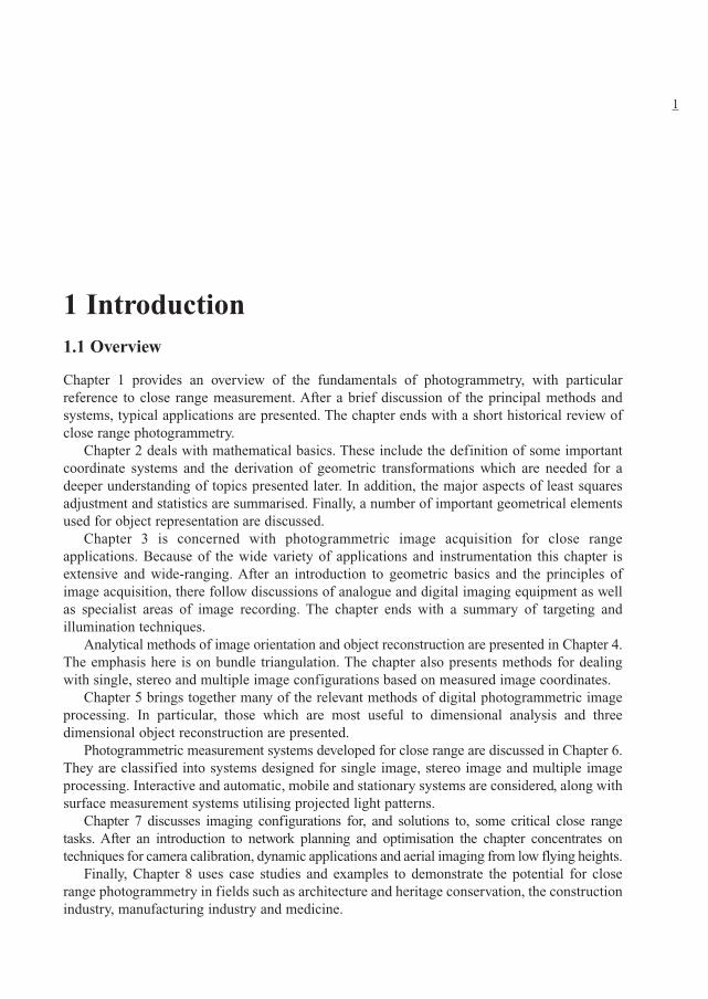
Photogrammetry encompasses methods of image measurement and interpretation in order toderive the shape and location of an object from one or more photographs of that object. Inprinciple, photogrammetric methods can be applied in any situation where the object to bemeasured can be photographically recorded. The primary purpose of a photogrammetricmeasurement is the three dimensional reconstruction of an object in digital form (coordinatesand derived geometric elements) or graphical form (images, drawings, maps). The photographor image represents a store of information which can be re-accessed at any time.

Fig. 1.1 shows examples of photogrammetric images. The reduction of a three-dimensional object to a two-dimensional image implies a loss of information. Object areaswhich are not visible in the image cannot be reconstructed from it. This not only includeshidden parts of an object such as the rear of a building but also regions which can not berecognised due to lack of contrast or limiting size, for example individual bricks in a buildingfaçade. Whereas the position in space of each point on the object may be defined by threecoordinates, there are only two coordinates available to define the position of its image. Thereare geometric changes caused by the shape of the object, the relative positioning of cameraand object, perspective imaging and optical lens defects. Finally there are also radiometric(colour) changes since the reflected electromagnetic radiation recorded in the image isaffected by the transmission media (air, glass) and the light-sensitive recording medium (film,electronic sensor).

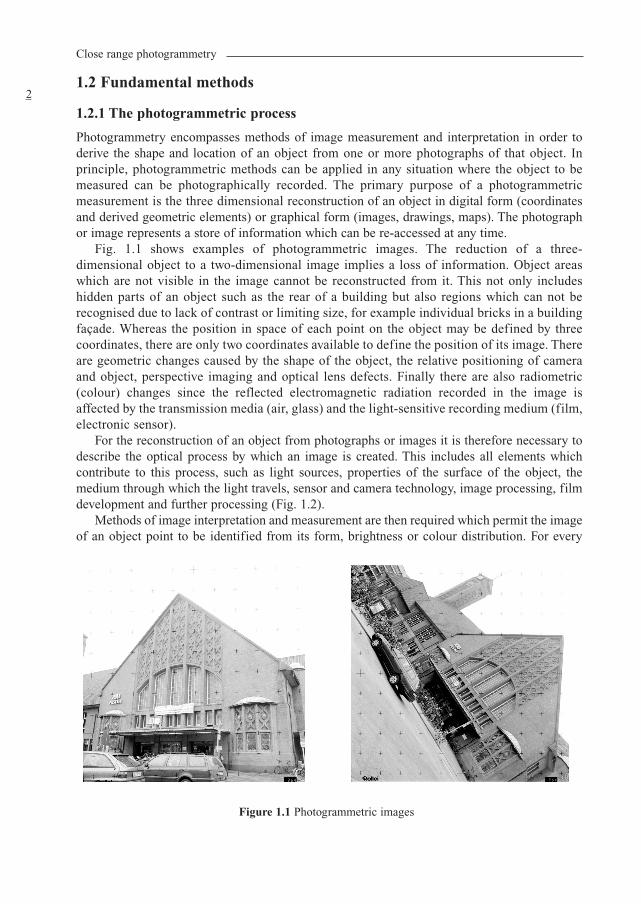
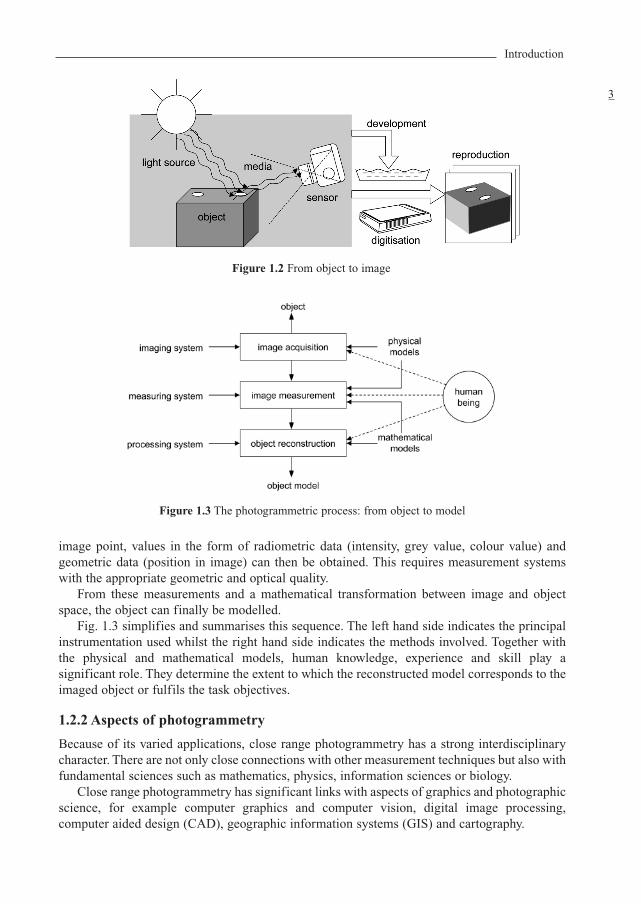
For the reconstruction of an object from photographs or images it is therefore necessary todescribe the optical process by which an image is created. This includes all elements whichcontribute to this process, such as light sources, properties of the surface of the object, themedium through which the light travels, sensor and camera technology, image processing, filmdevelopment and further processing (Fig. 1.2).

Methods of image interpretation and measurement are then required which permit the imageof an object point to be identified from its form, brightness or colour distribution. For every

Figure 1.1 Photogrammetric images

Introduction

3

Figure 1.2 From object to image

image point, values in the form of radiometric data (intensity, grey value, colour value) andgeometric data (position in image) can then be obtained. This requires measurement systemswith the appropriate geometric and optical quality.

From these measurements and a mathematical transformation between image and objectspace, the object can finally be modelled.

Fig. 1.3 simplifies and summarises this sequence. The left hand side indicates the principalinstrumentation used whilst the right hand side indicates the methods involved. Together withthe physical and mathematical models, human knowledge, experience and skill play asignificant role. They determine the extent to which the reconstructed model corresponds to theimaged object or fulfils the task objectives.

1.2.2 Aspects of photogrammetry

Because of its varied applications, close range photogrammetry has a strong interdisciplinarycharacter. There are not only close connections with other measurement techniques but also withfundamental sciences such as mathematics, physics, information sciences or biology.

Close range photogrammetry has significant links with aspects of graphics and photographicscience, for example computer graphics and computer vision, digital image processing,computer aided design (CAD), geographic information systems (GIS) and cartography.

Figure 1.3 The photogrammetric process: from object to model


4

Traditionally, there are also strong associations of close range photogrammetry with thetechniques of surveying, particularly in the areas of adjustment methods and engineeringsurveying. With the increasing application of photogrammetry to industrial metrology andquality control, links have been created in other directions.

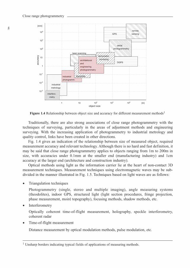
Fig. 1.4 gives an indication of the relationship between size of measured object, requiredmeasurement accuracy and relevant technology. Although there is no hard and fast definition, itmay be said that close range photogrammetry applies to objects ranging from 1m to 200m insize, with accuracies under 0.1mm at the smaller end (manufacturing industry) and 1cmaccuracy at the larger end (architecture and construction industry).

Optical methods using light as the information carrier lie at the heart of non-contact 3Dmeasurement techniques. Measurement techniques using electromagnetic waves may be sub-divided in the manner illustrated in Fig. 1.5. Techniques based on light waves are as follows:

• Triangulation techniques

Photogrammetry (single, stereo and multiple imaging), angle measuring systems(theodolites), indoor GPS, structured light (light section procedures, fringe projection,phase measurement, moiré topography), focusing methods, shadow methods, etc.

• Interferometry

Optically coherent time-of-flight measurement, holography, speckle interferometry,coherent radar

• Time-of-flight measurement

Distance measurement by optical modulation methods, pulse modulation, etc.

1 10 102 103 104

[mm]

[m]

10-2

10-3

10-1

1

10

102

103

104

accu

racy

object size

industrial

metrology

industrial

photogramm.

theodolite

aerial

photogrammetry

DGPS

tachymetric

surveying

GPS

remote

sensing

interfero-

metry

architektural

and

engineering

photogrammetry

laser scanning

Figure 1.4 Relationship between object size and accuracy for different measurement methods1

1 Unsharp borders indicating typical fields of applications of measuring methods.

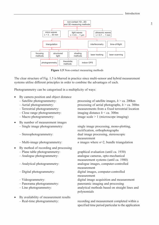
The clear structure of Fig. 1.5 is blurred in practice since multi-sensor and hybrid measurementsystems utilise different principles in order to combine the advantages of each.

Photogrammetry can be categorised in a multiplicity of ways:

• By camera position and object distance– Satellite photogrammetry: processing of satellite images, h > ca. 200km– Aerial photogrammetry: processing of aerial photographs, h > ca. 300m– Terrestrial photogrammetry: measurements from a fixed terrestrial location – Close range photogrammetry: imaging distance h < ca. 300m– Macro photogrammetry: image scale > 1 (microscope imaging)

• By number of measurement images– Single image photogrammetry: single image processing, mono-plotting,

rectification, orthophotographs– Stereophotogrammetry: dual image processing, stereoscopic

measurement– Multi-image photogrammetry: n images where n>2, bundle triangulation

• By method of recording and processing– Plane table photogrammetry: graphical evaluation (until ca. 1930)– Analogue photogrammetry: analogue cameras, opto-mechanical

measurement systems (until ca. 1980)– Analytical photogrammetry: analogue images, computer-controlled

measurement– Digital photogrammetry: digital images, computer-controlled

measurement– Videogrammetry: digital image acquisition and measurement– Panorama photogrammetry: panoramic imaging and processing– Line photogrammetry: analytical methods based on straight lines and

polynomials

• By availability of measurement results– Real-time photogrammetry: recording and measurement completed within a

specified time period particular to the application

Introduction

5non-contact 1D-, 2D-

and 3D measuring methods

light waves

λ = 0.5 ... 1 µm

micro waves

λ = 3 ... 30 mmultrasonic waves

λ = 0.1 ... 1 mm

interferometrytriangulation time-of-flight

photogrammetry

structured

light

focusing

methods

theodolite

methods

shading

methodslaser scanninglaser tracking

indoor GPS

Figure 1.5 Non-contact measuring methods

– Off-line photogrammetry: sequential, digital image recording, separatedin time or location from measurement

– On-line photogrammetry: simultaneous, multiple, digital image recording, immediate measurement

• By application or specialist area– Architectural photogrammetry: architecture, heritage conservation, archaeology– Engineering photogrammetry: general engineering (construction) applications– Industrial photogrammetry: industrial (manufacturing) applications– Forensic photogrammetry: applications to diverse legal problems– Biostereometrics: medical applications– Motography: recording moving target tracks– Multi-media photogrammetry: recording through media of different refractive

indices– Shape from stereo: stereo image processing (computer vision)

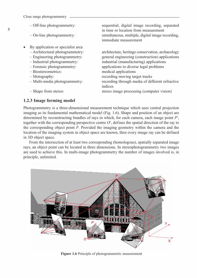
1.2.3 Image forming model

Photogrammetry is a three-dimensional measurement technique which uses central projectionimaging as its fundamental mathematical model (Fig. 1.6). Shape and position of an object aredetermined by reconstructing bundles of rays in which, for each camera, each image point P′,together with the corresponding perspective centre O′, defines the spatial direction of the ray tothe corresponding object point P. Provided the imaging geometry within the camera and thelocation of the imaging system in object space are known, then every image ray can be definedin 3D object space.

From the intersection of at least two corresponding (homologous), spatially separated imagerays, an object point can be located in three dimensions. In stereophotogrammetry two imagesare used to achieve this. In multi-image photogrammetry the number of images involved is, inprinciple, unlimited.


6

PP

P'P'

O'O'

ZZ

YY

XX

Figure 1.6 Principle of photogrammetric measurement

Introduction

7

1 In normal English, the orientation of an object implies direction or angular attitude. Photogrammetricusage, deriving from German, applies the word to groups of camera parameters. Exterior orientationparameters incorporate this angular meaning but extend it to include position. Interior orientationparameters, which include a distance, two coordinates and a number of polynomial coefficients, involveno angular values; the use of the terminology here underlines the connection between two very important,basic groups of parameters.

c

h

P

P'

O

x'

X

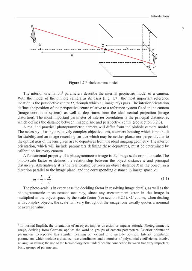
The interior orientation1 parameters describe the internal geometric model of a camera.With the model of the pinhole camera as its basis (Fig. 1.7), the most important referencelocation is the perspective centre O, through which all image rays pass. The interior orientationdefines the position of the perspective centre relative to a reference system fixed in the camera(image coordinate system), as well as departures from the ideal central projection (imagedistortion). The most important parameter of interior orientation is the principal distance, c,which defines the distance between image plane and perspective centre (see section 3.2.3).

A real and practical photogrammetric camera will differ from the pinhole camera model.The necessity of using a relatively complex objective lens, a camera housing which is not builtfor stability and an image recording surface which may be neither planar nor perpendicular tothe optical axis of the lens gives rise to departures from the ideal imaging geometry. The interiororientation, which will include parameters defining these departures, must be determined bycalibration for every camera.

A fundamental property of a photogrammetric image is the image scale or photo-scale. Thephoto-scale factor m defines the relationship between the object distance h and principaldistance c. Alternatively it is the relationship between an object distance X in the object, in adirection parallel to the image plane, and the corresponding distance in image space x′:

(1.1)

The photo-scale is in every case the deciding factor in resolving image details, as well as thephotogrammetric measurement accuracy, since any measurement error in the image ismultiplied in the object space by the scale factor (see section 3.2.1). Of course, when dealingwith complex objects, the scale will vary throughout the image; one usually quotes a nominalor average value.

mh

c

X

x= =

′

Figure 1.7 Pinhole camera model

The exterior orientation parameters specify the spatial position and orientation of the camerain a global coordinate system. The exterior orientation is described by the coordinates of theperspective centre in the global system and three suitably defined angles expressing the rotationof the image coordinate system with respect to the global system (see section 4.2.1). Theexterior orientation parameters are calculated indirectly, after measuring image coordinates ofwell identified object points with fixed and known global coordinates.

Every measured image point corresponds to a spatial direction from projection centre toobject point. The length of the direction vector is initially unknown i.e. every object point lyingon the line of this vector generates the same image point. In other words, although every threedimensional object point transforms to a unique image point for given orientation parameters,a unique reversal of the projection is not possible. The object point can be located on the imageray, and thereby absolutely determined in object space, only by intersecting the ray with anadditional known geometric element such as a second spatial direction or an object plane.

Every image generates a spatial bundle of rays, defined by the imaged points and theperspective centre, in which the rays were all recorded at the same point in time. If all thebundles of rays from multiple images are intersected as described above, a dense network iscreated; for an appropriate imaging configuration, such a network has the potential for highgeometric strength. Using the method of bundle triangulation any number of images (raybundles) can be simultaneously oriented, together with the calculation of the associated threedimensional object point locations (Fig. 1.6, see section 4.3).

1.2.4 Photogrammetric systems

1.2.4.1 Analogue systems

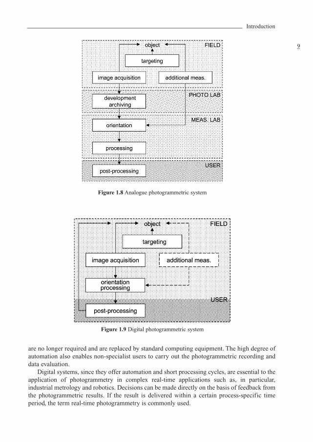
Analogue photogrammetry (Fig. 1.8) is distinguished by different instrumentation componentsfor data recording and for data processing as well as by a separation in location, time andpersonnel between the on-site recording of the object and the data evaluation in the laboratoryor office. Preparatory work and targeting, additional (surveying) measurement and imagerecording with expensive analogue (film or plate) cameras take place on site. Photographicdevelopment takes place in a laboratory, so that direct, on-site control of image quality isnot possible. Subsequently the photographs are measured using specialised instruments. Theprocedure involves firstly a determination of photo orientation followed by the actualprocessing of the photographic data.

The data obtained photogrammetrically are often further processed by users who do not wishto be involved in the actual measurement process since it requires complex photogrammetricknowledge, instrumentation and skills. The entire procedure, involving recording, measurementand further processing, is very time consuming using analogue systems, and many essentialstages cannot be completed on site. Direct integration of analogue systems in procedures suchas manufacturing processes is not possible.

1.2.4.2 Digital systems

The photogrammetric procedure has changed fundamentally with the development of digitalimaging systems and processing (Fig. 1.9). By utilising appropriately targeted object pointsand digital on-line image recording, complex photogrammetric tasks can be executed withinminutes on-site. A fully automatic analysis of the targeted points replaces the manualprocedures for orientation and measurement. Special photogrammetric measuring instruments


8

Introduction

9

Figure 1.8 Analogue photogrammetric system

Figure 1.9 Digital photogrammetric system

are no longer required and are replaced by standard computing equipment. The high degree ofautomation also enables non-specialist users to carry out the photogrammetric recording anddata evaluation.

Digital systems, since they offer automation and short processing cycles, are essential to theapplication of photogrammetry in complex real-time applications such as, in particular,industrial metrology and robotics. Decisions can be made directly on the basis of feedback fromthe photogrammetric results. If the result is delivered within a certain process-specific timeperiod, the term real-time photogrammetry is commonly used.


10

targeting

image recording

Recording

control points /

scaling lengths

development

and printing

image numbering

and archiving computation

digitising

image point

measurement

approximation

bundle

adjustment

removal of

outliers

coordinates of

object points

single point

measurement

exterior

orientations

graphical

plotting

interior

orientations

rectification /

orthophoto

Pre-processing

Orientation

Measurement &

analysis

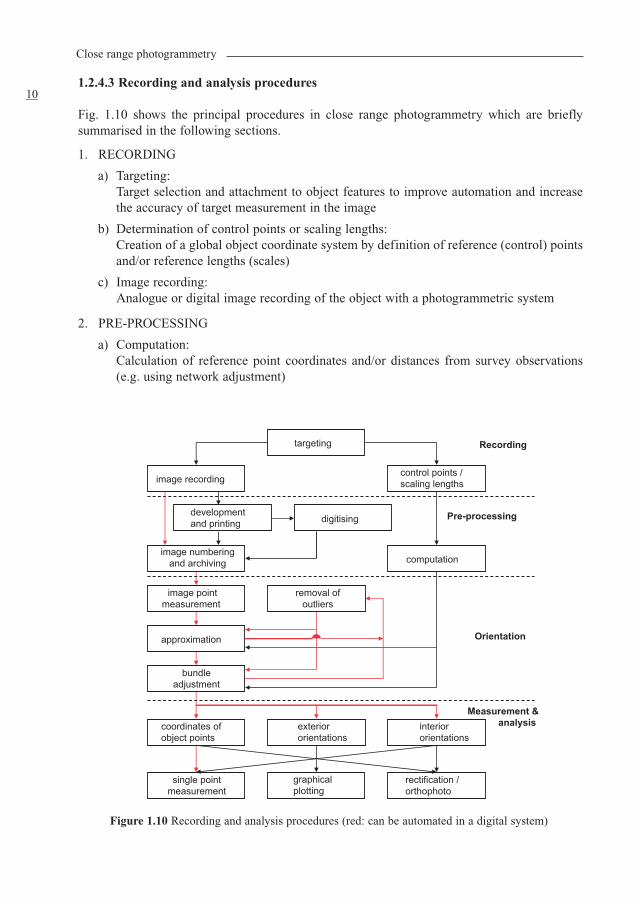
1.2.4.3 Recording and analysis procedures

Fig. 1.10 shows the principal procedures in close range photogrammetry which are brieflysummarised in the following sections.

1. RECORDING

a) Targeting:Target selection and attachment to object features to improve automation and increasethe accuracy of target measurement in the image

b) Determination of control points or scaling lengths:Creation of a global object coordinate system by definition of reference (control) pointsand/or reference lengths (scales)

c) Image recording:Analogue or digital image recording of the object with a photogrammetric system

2. PRE-PROCESSING

a) Computation:Calculation of reference point coordinates and/or distances from survey observations(e.g. using network adjustment)

Figure 1.10 Recording and analysis procedures (red: can be automated in a digital system)

b) Development and printing:Photographic laboratory work (developing film, making photographic prints)

c) Digitising:Conversion of analogue photographs into digital images (scanning)

d) Numbering and archiving:Assigning photo numbers to identify individual images and archiving or storing thephotographs

3. ORIENTATION

a) Measurement of image points:Identification and measurement of reference and scale pointsIdentification and measurement of tie points (points observed in two or more imagessimply to strengthen the network)

b) Approximation:Calculation of approximate (starting) values for unknown quantities to be calculated bythe bundle adjustment

c) Bundle adjustment:Adjustment program which simultaneously calculates parameters of both interior andexterior orientation as well as the object point coordinates which are required forsubsequent analysis

d) Removal of outliers:Detection and removal of gross errors which mainly arise during (manual) measurementof image points

4. MEASUREMENT AND ANALYSIS

a) Single point measurement:Creation of three dimensional object point coordinates for further numerical processing

b) Graphical plotting:Production of scaled maps or plans in analogue or digital form (e.g. hard copies for mapsand electronic files for CAD models or GIS)

c) Rectification/Orthophoto:Generation of transformed images or image mosaics which remove the effects of tiltrelative to a reference plane (rectification) and/or remove the effects of perspective(orthophoto)

This sequence can, to a large extent, be automated (connections in red in Fig. 1.10). Providedthat the object features are suitably marked and identified using coded targets, initial values canbe calculated and measurement outliers (gross errors) removed by robust estimation methods.

Digital image recording and processing can provide a self-contained and fast data flow fromcapture to presentation of results, so that object dimensions are available directly on site. Onedistinguishes between off-line photogrammetry systems (one camera, measuring resultavailable after processing of all acquired images), and on-line photogrammetry systems(minimum of two cameras simultaneously, measuring result immediately).

1.2.5 Photogrammetric products

In general, photogrammetric systems supply three dimensional object coordinates derived fromimage measurements. From these, further elements and dimensions can be derived, for example

Introduction

11

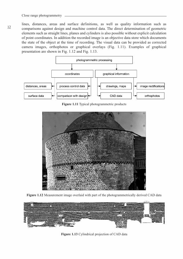
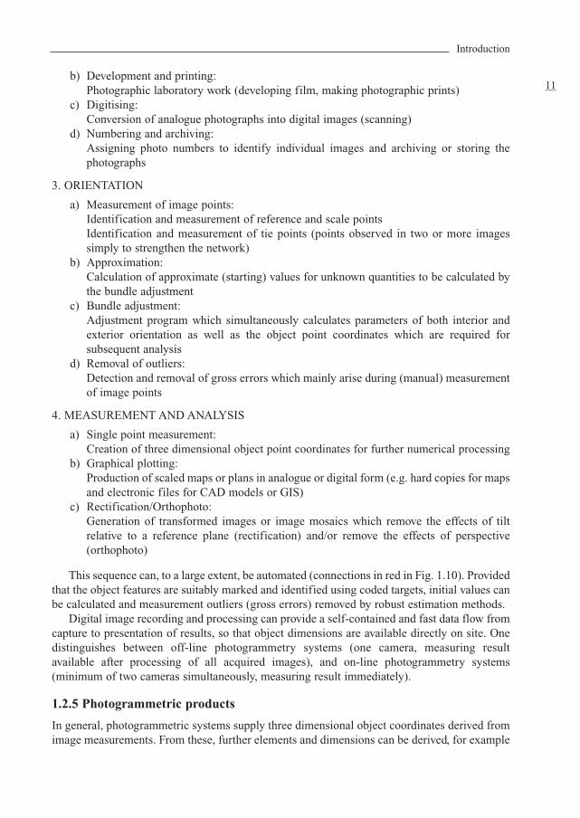
lines, distances, areas and surface definitions, as well as quality information such ascomparisons against design and machine control data. The direct determination of geometricelements such as straight lines, planes and cylinders is also possible without explicit calculationof point coordinates. In addition the recorded image is an objective data store which documentsthe state of the object at the time of recording. The visual data can be provided as correctedcamera images, orthophotos or graphical overlays (Fig. 1.11). Examples of graphicalpresentation are shown in Fig. 1.12 and Fig. 1.13.


12

Figure 1.13 Cylindrical projection of CAD data

Figure 1.12 Measurement image overlaid with part of the photogrammetrically derived CAD data

Figure 1.11 Typical photogrammetric products

1.3 Applications

Much shorter imaging ranges and alternative recording techniques differentiate close rangephotogrammetry from its aerial and satellite equivalents.

Writing in 1962 E. H. Thompson summarised the conditions under which photogrammetricmethods of measurement would be useful:

“... first, when the object to be measured is inaccessible or difficult of access; second, whenthe object is not rigid and its instantaneous dimensions are required; third, when it is not certainthat the measures will be required at all; fourth, when it is not certain, at the time ofmeasurement, what measures are required; and fifth, when the object is very small ...”.

To these may be added three more: when the use of direct measurement would influence themeasured object or would disturb a procedure going on around the object; when real-timeresults are required; and when the simultaneous recording and the measurement of a very largenumber of points is required.

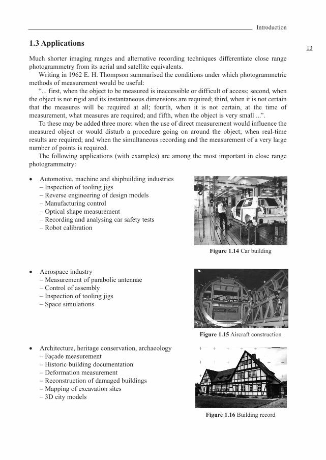
The following applications (with examples) are among the most important in close rangephotogrammetry:

• Automotive, machine and shipbuilding industries– Inspection of tooling jigs– Reverse engineering of design models– Manufacturing control– Optical shape measurement– Recording and analysing car safety tests– Robot calibration

• Aerospace industry– Measurement of parabolic antennae– Control of assembly– Inspection of tooling jigs– Space simulations

• Architecture, heritage conservation, archaeology– Façade measurement– Historic building documentation– Deformation measurement– Reconstruction of damaged buildings– Mapping of excavation sites– 3D city models

Introduction

13

Figure 1.14 Car building

Figure 1.15 Aircraft construction

Figure 1.16 Building record

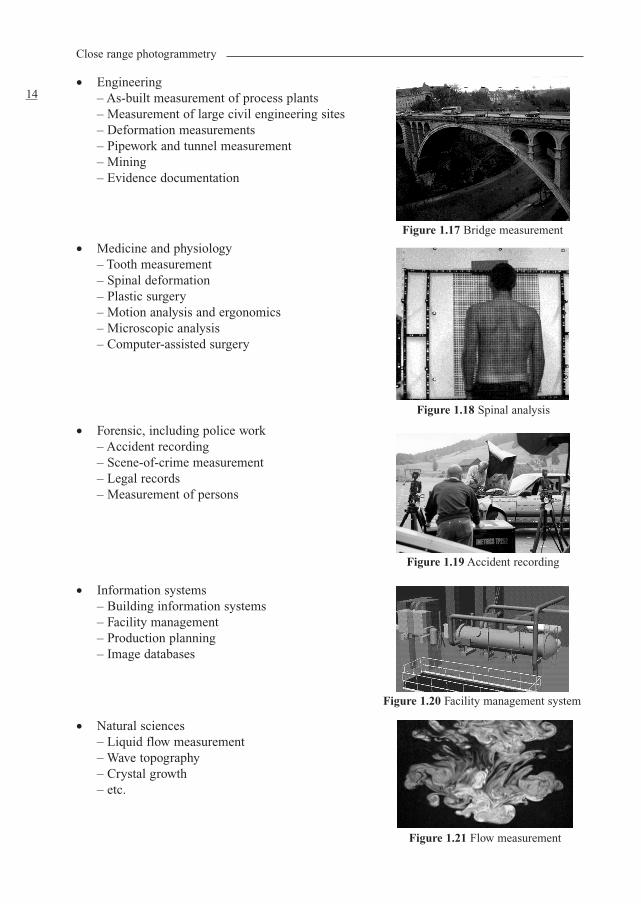
• Engineering– As-built measurement of process plants– Measurement of large civil engineering sites– Deformation measurements– Pipework and tunnel measurement– Mining– Evidence documentation

• Medicine and physiology– Tooth measurement– Spinal deformation– Plastic surgery– Motion analysis and ergonomics– Microscopic analysis– Computer-assisted surgery

• Forensic, including police work– Accident recording– Scene-of-crime measurement– Legal records – Measurement of persons

• Information systems– Building information systems– Facility management– Production planning– Image databases

• Natural sciences– Liquid flow measurement– Wave topography– Crystal growth– etc.


14

Figure 1.17 Bridge measurement

Figure 1.18 Spinal analysis

Figure 1.19 Accident recording

Figure 1.20 Facility management system

Figure 1.21 Flow measurement

In general, similar methods of recording and analysis are used for all applications of close rangephotogrammetry.

• powerful analogue or digital recording systems

• freely chosen imaging configuration with almost unlimited numbers of photographs

• photo orientation based on the technique of bundle triangulation

• visual and digital analysis of the images

• presentation of results in the form of 3D coordinate files, CAD data, photographs or drawings

Industrial and engineering applications make special demands of the photogrammetrictechnique:

• limited recording time on site (no significant interruption of industrial processes)

• delivery of results for analysis after only a brief time

• high accuracy requirements

• proof of accuracy attained

1.4 Historical development

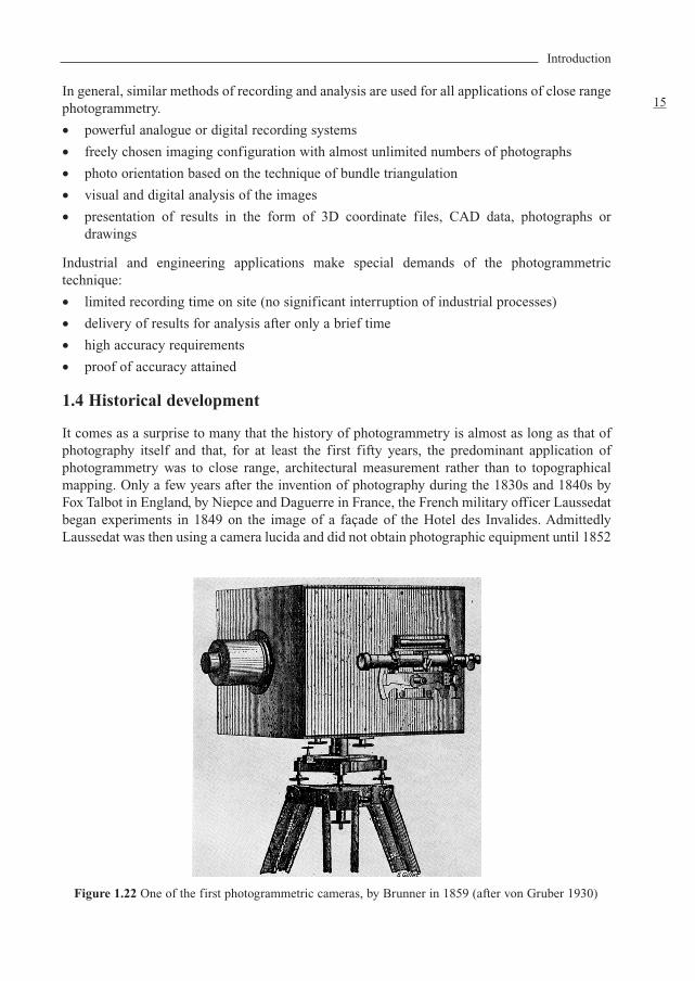
It comes as a surprise to many that the history of photogrammetry is almost as long as that ofphotography itself and that, for at least the first fifty years, the predominant application ofphotogrammetry was to close range, architectural measurement rather than to topographicalmapping. Only a few years after the invention of photography during the 1830s and 1840s byFox Talbot in England, by Niepce and Daguerre in France, the French military officer Laussedatbegan experiments in 1849 on the image of a façade of the Hotel des Invalides. AdmittedlyLaussedat was then using a camera lucida and did not obtain photographic equipment until 1852

Introduction

15

Figure 1.22 One of the first photogrammetric cameras, by Brunner in 1859 (after von Gruber 1930)

(Poivilliers 1961); he is usually described as the first photogrammetrist. In fact it was not asurveyor but an architect, the German Meydenbauer, who coined the word “photogrammetry”.As early as 1858 Meydenbauer used photographs to draw plans of the cathedral of Wetzlar andby 1865 he had constructed his “great photogrammeter” (Meydenbauer 1912), a forerunner ofthe phototheodolite.

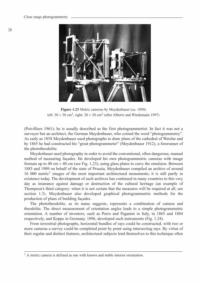
Meydenbauer used photography in order to avoid the conventional, often dangerous, manualmethod of measuring façades. He developed his own photogrammetric cameras with imageformats up to 40 cm × 40 cm (see Fig. 1.23), using glass plates to carry the emulsion. Between1885 and 1909 on behalf of the state of Prussia, Meydenbauer compiled an archive of around16 000 metric1 images of the most important architectural monuments; it is still partly inexistence today. The development of such archives has continued in many countries to this veryday as insurance against damage or destruction of the cultural heritage (an example ofThompson’s third category: when it is not certain that the measures will be required at all, seesection 1.3). Meydenbauer also developed graphical photogrammetric methods for theproduction of plans of building façades.

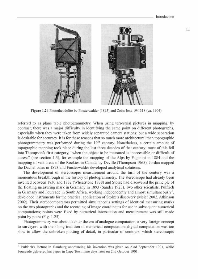
The phototheodolite, as its name suggests, represents a combination of camera andtheodolite. The direct measurement of orientation angles leads to a simple photogrammetricorientation. A number of inventors, such as Porro and Paganini in Italy, in 1865 and 1884respectively, and Koppe in Germany, 1896, developed such instruments (Fig. 1.24).

From terrestrial photographs, horizontal bundles of rays could be constructed; with two ormore cameras a survey could be completed point by point using intersecting rays. By virtue oftheir regular and distinct features, architectural subjects lend themselves to this technique often


16

Figure 1.23 Metric cameras by Meydenbauer (ca. 1890)

left: 30 × 30 cm2, right: 20 × 20 cm2 (after Albertz and Wiedemann 1997)

1 A metric camera is defined as one with known and stable interior orientation.

referred to as plane table photogrammetry. When using terrestrial pictures in mapping, bycontrast, there was a major difficulty in identifying the same point on different photographs,especially when they were taken from widely separated camera stations; but a wide separationis desirable for accuracy. It is for these reasons that so much more architectural than topographicphotogrammetry was performed during the 19th century. Nonetheless, a certain amount oftopographic mapping took place during the last three decades of that century; most of this fellinto Thompson’s first category, “when the object to be measured is inaccessible or difficult ofaccess” (see section 1.3), for example the mapping of the Alps by Paganini in 1884 and themapping of vast areas of the Rockies in Canada by Deville (Thompson 1965). Jordan mappedthe Dachel oasis in 1873 and Finsterwalder developed analytical solutions.

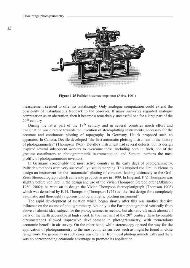
The development of stereoscopic measurement around the turn of the century was amomentous breakthrough in the history of photogrammetry. The stereoscope had already beeninvented between 1830 and 1832 (Wheatstone 1838) and Stolze had discovered the principle ofthe floating measuring mark in Germany in 1893 (Sander 1923). Two other scientists, Pulfrichin Germany and Fourcade in South Africa, working independently and almost simultaneously1,developed instruments for the practical application of Stolze’s discovery (Meier 2002, Atkinson2002). Their stereocomparators permitted simultaneous settings of identical measuring markson the two photographs and the recording of image coordinates for use in subsequent numericalcomputations; points were fixed by numerical intersection and measurement was still madepoint by point (Fig. 1.25).

Photogrammetry was about to enter the era of analogue computation, a very foreign conceptto surveyors with their long tradition of numerical computation: digital computation was tooslow to allow the unbroken plotting of detail, in particular of contours, which stereoscopic

Introduction

17

Figure 1.24 Phototheodolite by Finsterwalder (1895) and Zeiss Jena 19/1318 (ca. 1904)

1 Pulfrich’s lecture in Hamburg announcing his invention was given on 23rd September 1901, whileFourcade delivered his paper in Cape Town nine days later on 2nd October 1901.

measurement seemed to offer so tantalisingly. Only analogue computation could extend thepossibility of instantaneous feedback to the observer. If many surveyors regarded analoguecomputation as an aberration, then it became a remarkably successful one for a large part of the20th century.

During the latter part of the 19th century and in several countries much effort andimagination was directed towards the invention of stereoplotting instruments, necessary for theaccurate and continuous plotting of topography. In Germany, Hauck proposed such anapparatus. In Canada, Deville developed “the first automatic plotting instrument in the historyof photogrammetry” (Thompson 1965). Deville’s instrument had several defects, but its designinspired several subsequent workers to overcome these, including both Pulfrich, one of thegreatest contributors to photogrammetric instrumentation, and Santoni, perhaps the mostprolific of photogrammetric inventors.

In Germany, conceivably the most active country in the early days of photogrammetry,Pulfrich’s methods were very successfully used in mapping. This inspired von Orel in Vienna todesign an instrument for the “automatic” plotting of contours, leading ultimately to the Orel-Zeiss Stereoautograph which came into productive use in 1909. In England, F. V. Thompson wasslightly before von Orel in the design and use of the Vivian Thompson Stereoplotter (Atkinson1980, 2002); he went on to design the Vivian Thompson Stereoplanigraph (Thomson 1908)which was described by E. H. Thompson (Thompson 1974) as “the first design for a completelyautomatic and thoroughly rigorous photogrammetric plotting instrument”.

The rapid development of aviation which began shortly after this was another decisiveinfluence on the course of photogrammetry. Not only is the Earth photographed vertically fromabove an almost ideal subject for the photogrammetric method, but also aircraft made almost allparts of the Earth accessible at high speed. In the first half of the 20th century these favourablecircumstances allowed impressive development in photogrammetry, with tremendouseconomic benefit in air survey. On the other hand, while stereoscopy opened the way for theapplication of photogrammetry to the most complex surfaces such as might be found in closerange work, the geometry in such cases was often far from ideal photogrammetrically and therewas no corresponding economic advantage to promote its application.


18

Figure 1.25 Pulfrich’s stereocomparator (Zeiss, 1901)

Although there was considerable opposition from surveyors to the use of photographs andanalogue instruments for mapping, the development of stereoscopic measuring instrumentsforged ahead remarkably in many countries during the period between the First World War andthe early 1930s. Meanwhile, non-topographic use was sporadic as there were few suitablecameras and analogue plotters imposed severe restrictions on principal distance, imageformat and disposition and tilts of cameras. Instrumentally complex systems were beingdeveloped using optical projection (for example Multiplex), opto-mechanical principles (ZeissStereoplanigraph) and mechanical projection using space rods (for example Wild A5, SantoniStereocartograph), designed for use with aerial photography. By 1930 the Stereoplanigraph C5was in production, a sophisticated instrument able to use oblique and convergent photography—even if makeshift cameras had to be used at close range, experimenters at least had freedom in theorientation and placement of the cameras; this considerable advantage led to some noteworthywork.

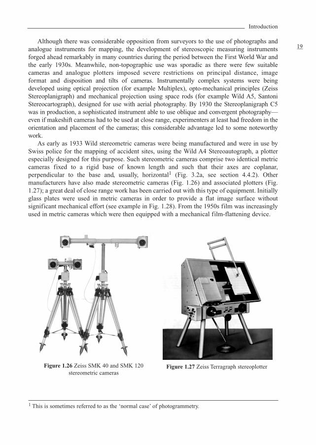
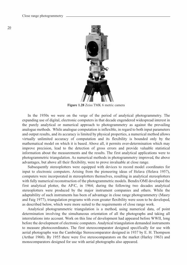
As early as 1933 Wild stereometric cameras were being manufactured and were in use bySwiss police for the mapping of accident sites, using the Wild A4 Stereoautograph, a plotterespecially designed for this purpose. Such stereometric cameras comprise two identical metriccameras fixed to a rigid base of known length and such that their axes are coplanar,perpendicular to the base and, usually, horizontal1 (Fig. 3.2a, see section 4.4.2). Othermanufacturers have also made stereometric cameras (Fig. 1.26) and associated plotters (Fig.1.27); a great deal of close range work has been carried out with this type of equipment. Initiallyglass plates were used in metric cameras in order to provide a flat image surface withoutsignificant mechanical effort (see example in Fig. 1.28). From the 1950s film was increasinglyused in metric cameras which were then equipped with a mechanical film-flattening device.

Introduction

19

Figure 1.26 Zeiss SMK 40 and SMK 120 stereometric cameras

Figure 1.27 Zeiss Terragraph stereoplotter

1 This is sometimes referred to as the ‘normal case’ of photogrammetry.

In the 1950s we were on the verge of the period of analytical photogrammetry. Theexpanding use of digital, electronic computers in that decade engendered widespread interest inthe purely analytical or numerical approach to photogrammetry as against the prevailinganalogue methods. While analogue computation is inflexible, in regard to both input parametersand output results, and its accuracy is limited by physical properties, a numerical method allowsvirtually unlimited accuracy of computation and its flexibility is bounded only by themathematical model on which it is based. Above all, it permits over-determination which mayimprove precision, lead to the detection of gross errors and provide valuable statisticalinformation about the measurements and the results. The first analytical applications were tophotogrammetric triangulation. As numerical methods in photogrammetry improved, the aboveadvantages, but above all their flexibility, were to prove invaluable at close range.

Subsequently stereoplotters were equipped with devices to record model coordinates forinput to electronic computers. Arising from the pioneering ideas of Helava (Helava 1957),computers were incorporated in stereoplotters themselves, resulting in analytical stereoplotterswith fully numerical reconstruction of the photogrammetric models. Bendix/OMI developed thefirst analytical plotter, the AP/C, in 1964; during the following two decades analyticalstereoplotters were produced by the major instrument companies and others. While theadaptability of such instruments has been of advantage in close range photogrammetry (Masryand Faig 1977), triangulation programs with even greater flexibility were soon to be developed,as described below, which were more suited to the requirements of close range work.

Analytical photogrammetric triangulation is a method, using numerical data, of pointdetermination involving the simultaneous orientation of all the photographs and taking allinterrelations into account. Work on this line of development had appeared before WWII, longbefore the development of electronic computers. Analytical triangulation demanded instrumentsto measure photocoordinates. The first stereocomparator designed specifically for use withaerial photographs was the Cambridge Stereocomparator designed in 1937 by E. H. Thompson(Arthur 1960). By 1955 there were five stereocomparators on the market (Harley 1963) andmonocomparators designed for use with aerial photographs also appeared.


20

Figure 1.28 Zeiss TMK 6 metric camera

The bundle method of photogrammetric triangulation, more usually known as bundleadjustment, is of vital importance to close range photogrammetry. Seminal papers by Schmid(1956-57, 1958) and Brown (1958) laid the foundations for theoretically rigorous blockadjustment. A number of bundle adjustment programs for air survey were developed andbecame commercially available, such as those by Ackermann et al. (1970) and Brown (1976).Programs designed specifically for close range work have appeared since the 1980s, such asSTARS (Fraser and Brown 1986), BINGO (Kruck 1983), MOR (Wester-Ebbinghaus 1981) andCAP (Hinsken 1989).

The importance of bundle adjustment in close range photogrammetry can hardly be overstated.The method imposes no restrictions on the positions or the orientations of the cameras; nor is thereany necessity to limit the imaging system to central projection. Of equal or greater importance, theparameters of interior orientation of all the cameras may be included as unknowns in the solution.Until the 1960s many experimenters appear to have given little attention to the calibration1 of theircameras; this may well have been because the direct calibration of cameras focused for nearobjects is usually much more difficult than that of cameras focused for distant objects. At the sametime, the inner orientation must usually be known more accurately than is necessary for verticalaerial photographs because the geometry of non-topographical work is frequently far from ideal.In applying the standard methods of calibration in the past, difficulties arose because of the finitedistance of the targets, whether real objects or virtual images. While indirect, numerical methodsto overcome this difficulty were suggested by Torlegård (1967) and others, bundle adjustment nowfrees us from this concern. For high precision work it is no longer necessary to use metric cameraswhich, while having the advantage of known and constant interior orientation, are usuallycumbersome and expensive. Virtually any camera can now be used. Calibration via bundleadjustment is usually known as self-calibration (see section 4.3.2.4).

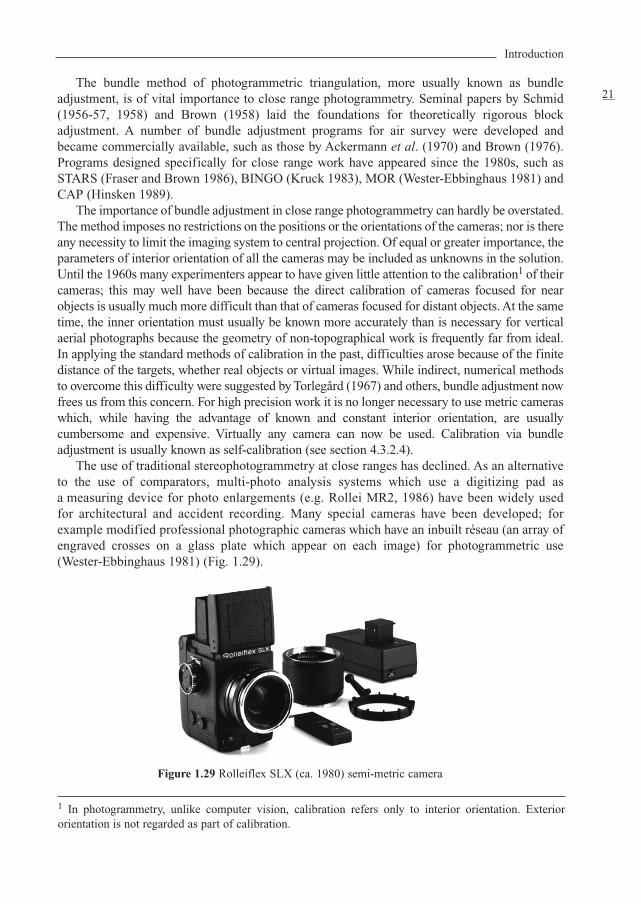
The use of traditional stereophotogrammetry at close ranges has declined. As an alternativeto the use of comparators, multi-photo analysis systems which use a digitizing pad asa measuring device for photo enlargements (e.g. Rollei MR2, 1986) have been widely usedfor architectural and accident recording. Many special cameras have been developed; forexample modified professional photographic cameras which have an inbuilt réseau (an array ofengraved crosses on a glass plate which appear on each image) for photogrammetric use(Wester-Ebbinghaus 1981) (Fig. 1.29).

Introduction

21

Figure 1.29 Rolleiflex SLX (ca. 1980) semi-metric camera

1 In photogrammetry, unlike computer vision, calibration refers only to interior orientation. Exteriororientation is not regarded as part of calibration.

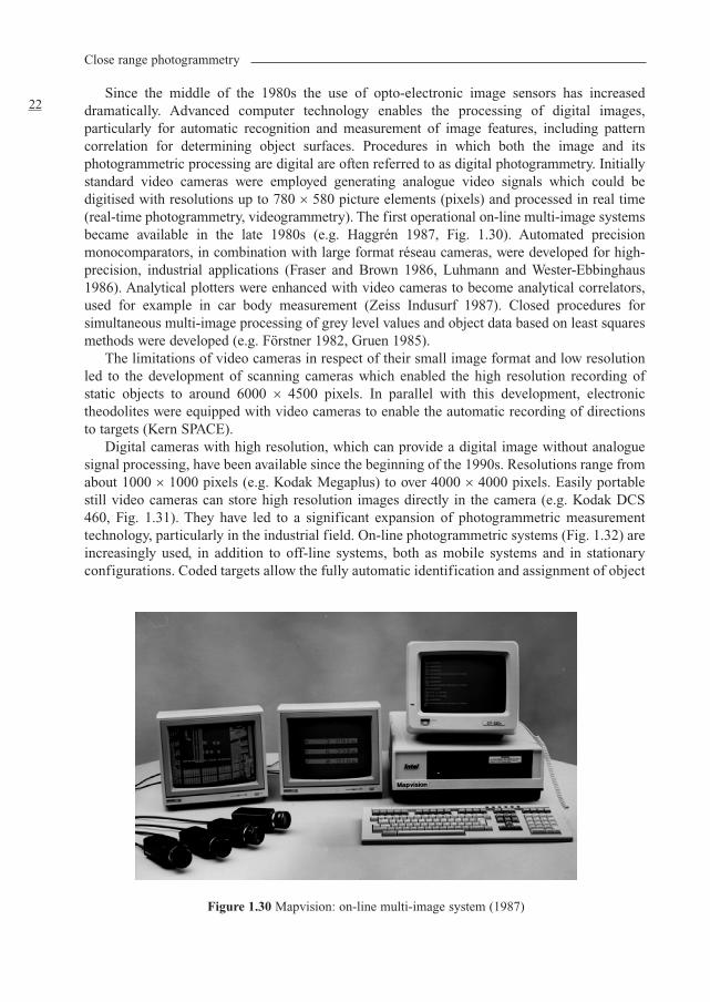
Since the middle of the 1980s the use of opto-electronic image sensors has increaseddramatically. Advanced computer technology enables the processing of digital images,particularly for automatic recognition and measurement of image features, including patterncorrelation for determining object surfaces. Procedures in which both the image and itsphotogrammetric processing are digital are often referred to as digital photogrammetry. Initiallystandard video cameras were employed generating analogue video signals which could bedigitised with resolutions up to 780 × 580 picture elements (pixels) and processed in real time(real-time photogrammetry, videogrammetry). The first operational on-line multi-image systemsbecame available in the late 1980s (e.g. Haggrén 1987, Fig. 1.30). Automated precisionmonocomparators, in combination with large format réseau cameras, were developed for high-precision, industrial applications (Fraser and Brown 1986, Luhmann and Wester-Ebbinghaus1986). Analytical plotters were enhanced with video cameras to become analytical correlators,used for example in car body measurement (Zeiss Indusurf 1987). Closed procedures forsimultaneous multi-image processing of grey level values and object data based on least squaresmethods were developed (e.g. Förstner 1982, Gruen 1985).

The limitations of video cameras in respect of their small image format and low resolutionled to the development of scanning cameras which enabled the high resolution recording ofstatic objects to around 6000 × 4500 pixels. In parallel with this development, electronictheodolites were equipped with video cameras to enable the automatic recording of directionsto targets (Kern SPACE).

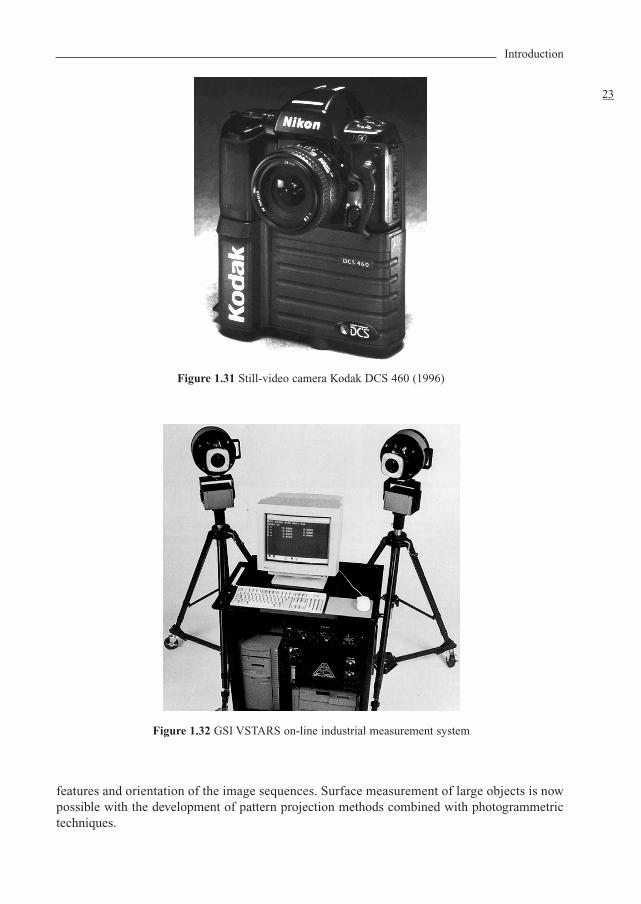
Digital cameras with high resolution, which can provide a digital image without analoguesignal processing, have been available since the beginning of the 1990s. Resolutions range fromabout 1000 × 1000 pixels (e.g. Kodak Megaplus) to over 4000 × 4000 pixels. Easily portablestill video cameras can store high resolution images directly in the camera (e.g. Kodak DCS460, Fig. 1.31). They have led to a significant expansion of photogrammetric measurementtechnology, particularly in the industrial field. On-line photogrammetric systems (Fig. 1.32) areincreasingly used, in addition to off-line systems, both as mobile systems and in stationaryconfigurations. Coded targets allow the fully automatic identification and assignment of object


22

Figure 1.30 Mapvision: on-line multi-image system (1987)

features and orientation of the image sequences. Surface measurement of large objects is nowpossible with the development of pattern projection methods combined with photogrammetrictechniques.

Introduction

23

Figure 1.31 Still-video camera Kodak DCS 460 (1996)

Figure 1.32 GSI VSTARS on-line industrial measurement system

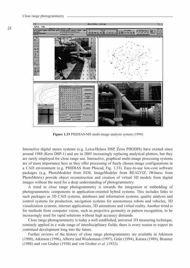
Interactive digital stereo systems (e.g. Leica/Helava DSP, Zeiss PHODIS) have existed sincearound 1988 (Kern DSP-1) and are in 2005 increasingly replacing analytical plotters, but theyare rarely employed for close range use. Interactive, graphical multi-image processing systemsare of more importance here as they offer processing of freely chosen image configurations ina CAD environment (e.g. PHIDIAS from Phocad, Fig. 1.33). Easy-to-use low-cost softwarepackages (e.g. PhotoModeler from EOS, ImageModeler from REALVIZ, iWitness fromPhotoMetrix) provide object reconstruction and creation of virtual 3D models from digitalimages without the need for a deep understanding of photogrammetry.

A trend in close range photogrammetry is towards the integration or embedding ofphotogrammetric components in application-oriented hybrid systems. This includes links tosuch packages as 3D CAD systems, databases and information systems, quality analysis andcontrol systems for production, navigation systems for autonomous robots and vehicles, 3Dvisualization systems, internet applications, 3D animations and virtual reality. Another trend isfor methods from computer vision, such as projective geometry or pattern recognition, to beincreasingly used for rapid solutions without high accuracy demands.

Close range photogrammetry is today a well established, universal 3D measuring technique,routinely applied in a wide range of interdisciplinary fields; there is every reason to expect itscontinued development long into the future.

Further reviews of the history of close range photogrammetry are available in Atkinson(1980), Atkinson (1996), Albertz and Wiedemann (1997), Grün (1994), Karara (1989), Brunner(1988) and von Gruber (1930) and von Gruber et al. (1932).


24

Figure 1.33 PHIDIAS-MS multi-image analysis system (1998)

References

Ackermann, F., Ebner, H. and Klein, H. (1970) Ein Rechenprogramm für die Streifentriangulationmit unabhängigen Modellen. Bildmessung und Luftbildwesen, Heft 4/1970, pp. 206–217.

Albertz, J. and Wiedemann, A. (ed.) (1997) Architekturphotogrammetrie gestern-heute-morgen.Technische Universität Berlin.

Arthur, D. W. G. (1960) An automatic recording stereocomparator. Photogrammetric Record3(16), 298–319.

Atkinson, K. B. (1980) Vivian Thompson (1880–1917) not only an officer in the RoyalEngineers. Photogrammetric Record, 10(55), 5–38.

Atkinson, K. B. (ed.) (1996) Close range photogrammetry and machine vision. WhittlesPublishing, Caithness, UK.

Atkinson, K. B. (2002) Fourcade: The Centenary – Response to Professor H.-K. Meier. Cor-respondence, Photogrammetric Record, 17(99), 555–556.

Brown, D. C. (1958) A solution to the general problem of multiple station analyticalstereotriangulation. RCA Data Reduction Technical Report No. 43, Aberdeen 1958.

Brown, D. C. (1976) The bundle adjustment – progress and prospects. International Archives ofPhotogrammetry, 21(3), ISP Congress, Helsinki, pp. 1–33.

Brunner, K. (1988) Die Meßtischphotogrammetrie als Methode der topographischenGeländeaufnahme des ausgehenden 19. Jahrhunderts. Zeitschrift für Photogrammetrie undFernerkundung, Heft 3/88, pp. 98–108.

Förstner, W. (1982) On the geometric precision of digital correlation. International Archives forPhotogrammetry and Remote Sensing, 26(3), 176–189.

Fraser, C. S. and Brown, D. C. (1986) Industrial photogrammetry – new developments andrecent applications. Photogrammetric Record, 12(68).

von Gruber, O. (ed.) (1930) Ferienkurs in Photogrammetrie. Verlag Konrad Wittwer, Stuttgart.von Gruber, O. (ed.), McCaw, G. T. and Cazalet, F. A., (trans) (1932) Photogrammetry, Collected

Lectures and Essays. Chapman & Hall, London.Gruen, A. (1985) Adaptive least squares correlation – a powerful image matching technique.

South African Journal of Photogrammetry, Remote Sensing and Cartography, 14(3), pp.175–187.

Grün, A. (1994) Von Meydenbauer zur Megaplus – Die Architekturphotogrammetrie im Spiegelder technischen Entwicklung. Zeitschrift für Photogrammetrie und Fernerkundung, Heft2/1994, pp. 41–56.

Haggrén, H. (1987) Real-time photogrammetry as used for machine vision applications.Canadian Surveyor, 41(2), pp. 210–208.

Harley, I. A. (1963) Some notes on stereocomparators. Photogrammetric Record, IV(21),194–209.

Helava, U. V. (1957) New principle for analytical plotters. Photogrammetria, 14, 89–96.Hinsken, L. (1989) CAP: Ein Programm zur kombinierten Bündelausgleichung auf

Personalcomputern. Zeitschrift für Photogrammetrie und Fernerkundung, Heft 3/1989, pp.92–95.

Karara, H. M. (ed.) (1989) Non-topographic photogrammetry. 2nd ed., American Society forPhotogrammetry and Remote Sensing.

Kruck, E. (1983) Lösung großer Gleichungssysteme für photogrammetrische Blockausg-leichungen mit erweitertem funktionalem Modell. Dissertation, Wiss. Arbeiten derFachrichtung Vermessungswesen der Universität Hannover, Nr. 128.

Luhmann, T. and Wester-Ebbinghaus, W. (1986) Rolleimetric RS – A New System for DigitalImage Processing. Symposium ISPRS Commission II, Baltimore.

Masry, S. E. and Faig, W. (1977) The Analytical Plotter in Close-Range Applications.Photogrammetric Engineering and Remote Sensing, January 1977.

Introduction

25

Meier, H.-K. (2002) Fourcade: The Centenary – Paper by L. P. Adams. Correspondence,Photogrammetric Record, 17(99), 554–555.

Meydenbauer, A. (1912) Handbuch der Messbildkunst. Knapp, Halle, 245p.Poivilliers, G. (1961) Address delivered at the opening of the Historical Exhibition, Ninth Inter-

national Congress of Photogrammetry, London, 1960. International Archives of Photo-grammetry, XIII, 1, 1961.

Sander, W. (1923) Die stereoskopischen Messverfahren. Zentralzeitung für Optik undMechanik, 44: 81–85, 96–100 and 110–114, Berlin.

Schmid, H. (1956–57) An analytical treatment of the problem of triangulation bystereophotogrammetry. Photogrammetria, XIII, Nr. 2 and 3.

Schmid, H. (1958) Eine allgemeine analytische Lösung für die Aufgabe der Photogrammetrie.Bildmessung and Luftbildwesen. 1958 Nr. 4 (103–113) and 1959 Nr. 1 (1–12).

Thompson, E. H. (1962) Photogrammetry. The Royal Engineers Journal, 76(4) 432–444.Reprinted in Photogrammetry and surveying, a selection of papers by E. H. Thompson,1910–1976. Photogrammetric Society, London, 1977.

Thompson, E. H. (1965) The Deville Memorial Lecture. The Canadian Surveyor, 19(3)262–272. Reprinted in Photogrammetry and surveying, a selection of papers by E. H.Thompson, 1910–1976. Photogrammetric Society, London, 1977.

Thompson, E. H. (1974) The Vivian Thompson Stereo-Planigraph. Photogrammetric Record,8(43) 81–86.

Thompson, V. F. (1908) Stereo-photo-surveying. The Geographical Journal, 31: p. 534.Torlegård, K. (1967) On the determination of interior orientation of close-up cameras under

operational conditions using three-dimensional test objects. Doctoral Thesis, Kungl.Tekniska Höskolan.

Wester-Ebbinghaus, W. (1981) Zur Verfahrensentwicklung in der Nahbereichsphoto-grammetrie.Dissertation, Bonn University.

Wheatstone, C. (1838) Contribution to the physiology of vision – Part the first. On someremarkable, and hitherto unobserved, phenomena of binocular vision. PhilosophicalTransactions of the Royal Society of London for the year MDCCCXXXVIII, Part II,371–94.

Further reading

Photogrammetry

Adams, L. P. (2001) Fourcade: The centenary of a stereoscopic method of photogrammetricsurveying. Photogrammetric Record, 17(99), 225–242.

Albertz, J. and Kreiling, W. (1989) Photogrammetric guide. 4th edition, Wichmann Verlag,Karlsruhe, Germany.

Atkinson, K. B. (ed.) (1980) Developments in close range photogrammetry-1. Applied SciencePublishers, London, UK.

Deville, E. (1895) Photographic Surveying. Government Printing Bureau, Ottawa. p. 232.Deville, E. (1902) On the use of the Wheatstone Stereoscope in Photographic Surveying.

Transactions of the Royal Society of Canada, Ottawa. 8: 63–69.Fourcade, H. G. (1903) On a stereoscopic method of photographic surveying. Transactions of

the South African Philosophical Society, 14(1) 28–35. (Also published in 1902. Nature, 66(1701) 139–141.)

Kraus, K. (1997) Photogrammetry, Volume 2, Advanced Methods and Applications. Withcontributions by J. Jansa and H. Kager. Dümmler, Bonn.

Kraus, K. (2000) Photogrammetry, Volume 1, Fundamentals and Standard Processes. Withcontributions by Peter Waldhäusl, translated by Peter Stewardson, Verlag H. Stam GmbH,Köln.


26

Kraus, K. (2004) Photogrammetrie, Band 1, Geometrische Informationen aus Photographienund Laserscanneraufnahmen. Walter de Gruyter, Berlin, 516 p.

Laussedat, A. (1898, 1901, 1903) Recherches sur les instruments, les méthodes et le dessintopographiques. Gauthier-Villars, Paris. (Vol. 1, 1898; Vol. 2 part 1, 1901: part 2 1903)

McGlone, J. C. (ed.) (2004) Manual of photogrammetry. 5th edition, American Society forPhotogrammetry and Remote Sensing.

Mikhail, E. M., Bethel, J. S. and McGlone, J. C. (2001) Introduction to Modern Photo-grammetry. John Wiley & Sons, New York.

Pulfrich, C. (1902) Über neuere Anwendungen der Stereoskopie und über einen hierfürbestimmten Stereo-Komparator. Zeitschrift für Instrumentenkunde, 22(3):65–81.

Schenk, T. (1999) Digital Photogrammetry, Vol. 1, TerraScience, Laurelville, USA. Thompson, M. M. (ed.) (1980) Manual of Photogrammetry. 4th edition, American Society for

Photogrammetry and Remote Sensing.

Optics, camera and image acquisition

Born, M., Wolf, E. and Bhatia, A. B. (1999) Principles of Optics. Cambridge University Press,p. 986.

Hecht, E. (2003) Optics. Addison Wesley.Holst, G. C. (1996) CCD arrays, cameras and displays. SPIE Press, JCD Publishing, USA.Inglis, A. F. and Luther, A. C. (1996) Video engineering. 2nd ed., McGraw-Hill, New York.Schwarte, R. (1997) Überblick und Vergleich aktueller Verfahren der optischen Formerfassung.

GMA-Bericht 30, Optische Formerfassung, Langen, pp. 1-12.

Digital image processing, computer vision and pattern recognition

Demant, C., Streicher-Abel, B. and Waszkewitz, (1999) Industrial image processing – Visualquality control in manufacturing. Springer, p. 353.

Gonzales, R. C. and Wintz, P. (1987) Digital Image Processing. 2nd edition, Addison Wesley,p. 503.

Gonzales, R.C. and Woods, R.E. (2003) Digital Image Processing. Prentice Hall, p. 813.Graham, R. (1998) Digital Imaging. Whittles Publishing, Caithness, Scotland, UK.Haralick, R. M. and Shapiro, L. G. (1992) Computer and robot vision. Vol. I+II, Addison-

Wesley, Reading, Ma., USA.Hartley, R. and Zisserman, A. (2000) Multiple View Geometry. Cambridge University Press,

Cambridge, UK.Jähne, B., Haußecker, H. and Geißler, P. (1999) Handbook of computer vision and applications;

Vol. 1 Sensors and imaging; Vol. 2 Signal processing and pattern recognition; Vol. 3Systems and applications. Academic Press.

Marr, D. (1982) Vision. Freeman, San Francisco.Parker, J. R. (1996) Algorithms for Image Processing and Computer Vision. John Wiley & Sons

Inc, p. 432.Rosenfeld, A. and Kak, A. C. (1982) Digital Picture Processing, 2nd edition, Academic Press.Russ, J. C. (2002) The Image Processing Handbook. CRC Press, p. 752.

3D computer graphics

Foley, J. D., VanDam, A. and Feiner, S. K. (1995) Computer Graphics. Addison-WesleyProfessional, p.1200.

Laszlo, M. J. (1996) Computational Geometry and Computer Graphics in C++, Prentice-Hall,Upper Saddle River, NJ, p. 266.

Introduction

27

Shirley, P. (2002) Fundamentals of Computer Graphics. A K Peters, pp. 500.Watt, A. (1999) 3D Computer Graphics. Addison Wesley Publishing, pp. 592.

Least squares adjustment and statistics

Cross, P. A. (1990) Working Paper No. 6, Advanced least squares applied to position-fixing.Department of Land Surveying, Polytechnic (now University) of East London p. 205.

Mikhail, E. M. (1976) Observations and least squares. IEP, New York, p. 497.Mikhail, E. M. and Gracie, G. (1981) Analysis & Adjustment of Survey Measurements. Van

Nostrand Reinhold Company, p. 368. Wolf, P. R. and Ghilani, C.D. (1997) Adjustment Computations: Statistics and Least Squares in

Surveying and GIS (Surveying & Boundary Control), John Wiley & Sons.

Applications

Fryer, J. G., Mitchell, H. L. and Chandler, J. H. (2006) Applications of 3D measurement fromimages. Whittles Publishing, Caithness, Scotland, UK.

Harley, I. A. (1967) The non-topographical uses of photogrammetry. The Australian Surveyor,21(7) 237–263.

Luhmann, T. (ed.) (2002) Nahbereichsphotogrammetrie in der Praxis. Wichmann, Heidelberg,318 p.

Santoni, E. (1966) Instruments and photogrammetric devices for survey of close-up subject withparticular stress to that of car bodies and their components photographed at variousdistances. Inedito. Reprinted in Selected Works, Ermenegildo Santoni, Scritti Scelti1925–1968. Società Italiana di Fotogrammetria e Topographia, Firenze, 1971.

Standards and guidelines

DIN 1319: Fundamentals of metrology. Beuth, Berlin.DIN 18716: Photogrammetry and remote sensing. Beuth, Berlin.DIN 18709: Concepts, abbreviations and symbols in surveying. Beuth, Berlin.GUM (1993) ISO guide to the expression of uncertainty in measurement (GUM).ISO 10360: Geometrical Product Specifications (GPS) - Acceptance and reverification tests for

coordinate measuring machines (CMM). Beuth, Berlin.VDI/VDE 2617: Accuracy of coordinate measuring machines; characteristics and their

checking. VDI/VDE guide line, Part 1–6, Beuth, Berlin.VDI/VDE 2634: Optical 3D measuring systems. VDI/VDE guide line, Beuth, Berlin.

Organisations, conferences and working groups

ISPRS (International Society for Photogrammetry and Remote Sensing):Commission III: Theory and AlgorithmsCommission V: Close range Techniques and Machine VisionPublications: International Archives of Photogrammetry and Remote Sensing; ISPRSJournal of Photogrammetry and Remote Sensingwww.isprs.org

ASPRS (The American Society for Photogrammetry and Remote Sensing): Publication: Photogrammetric Engineering and Remote Sensing www.asprs.org


28

The Remote Sensing and Photogrammetry Society: Publication: The Photogrammetric Recordwww.rspsoc.org

DGPF (Deutsche Gesellschaft für Photogrammetrie und Fernerkundung): Publications:Bildmessung und Luftbildwesen (to 1989), Zeitschrift für Photo-grammetrie undFernerkundung (to 1997), Photogrammetrie-Fernerkundung-Geoinformation (since1997); Publikationen der DGPF (proceedings of the annual symposia) www.dgpf.de

CIPA (Comité International de Photogrammétrie Architecturale): Publications and conference proceedings.http://cipa.icomos.org/

CMCS (Coordinate Metrology Systems Conference)Publications and conference proceedings.www.cmsc.org

SPIE (The International Society for Optical Engineering):Publications and conference proceedings.www.spie.org

VDI/VDE-GMA (VDI/VDE-Gesellschaft für Mess- und Automatisierungstechnik):Publications: technical guide lines, conference proceedings.www.vdi.de

Introduction

29

2½ D surface 903-2-1 method 247, 24935 mm camera 143, 165360° scanner 1763-chip method 1723D

circle 86, 88, 89digitiser 408Helmert transformation 45surface 90

4-parameter transformation 346-parameter transformation 356 DOF 214

Abbe’s comparator principle 401absolute orientation 227–29

datum definition 228–29model 227–28spatial point distribution 245

absorption 155acceptance

test 433–34, 442tolerance 434

accident record 489accuracy

contour method 290–91image measurement 442inner 250instruments 442length measurement 434, 436object point 99on-line systems 417normal stereo case 104self-calibration 263–64stereo image processing 275

acquisitionmulti-image 98, 99–100single image 98, 102

adapter 417, 489, 492additional

parameter functions 242parameters 120

adjustmentconditional least squares 58–59Gauss-Markov method 55least squares 34, 46, 55, 79of direct observations 55–56procedure 38reliability 64–66systems 43techniques 52–72

aerial image 465–66, 475, 489photogrammetry 5, 202triangulation 230

aerospace industry 13, 485affine transformations

matrix notation 36plane 35–36spatial similarity 44

affinity 114, 119, 120, 162, 243, 264airborne laser scanning 475aliasing 133, 154, 159all-round measurements 430altimeter 466amateur camera 127, 163, 165anaglyph 281, 410analogue photogrammetry 5, 8analogue-to-digital converter 161analysis procedures 10–11

Index

analytical photogrammetry 5, 20plotter 20, 407–09

angle of convergence 98angular resolution 310antenna measurement 447anti-aliasing filter 133aperture

depth of field 110–12lens 106, 107linear 106relative 112–13size 134, 153telecentric lenses 114

approximate values 46–483D transformation 46–48bundle adjustment 230, 234, 251–60functional model 54panorama orientation 311–12relative orientation 221, 226rotation parameters 211space resection 209

approximation 11, 83B-spline 80–81Bezier 81–82point 79surface 92

archaeology 6, 13, 466architectural photogrammetry 6, 469–77archiving 11artificial cooling 156as-built documentation 414, 484autobar 255auto-focus 165auto-stereoscopic display 410auxiliary coordinate system 241–42

B-spline 292approximation 80–81surface 81, 93

background intensity 426noise 156

balancedobservations 447 radial distortion 117

ball plate 435, 436band

absorption technique 464interleaved 323

band-pass filter 133barcode 188basal plane 217base see stereobasebase components 219, 220, 229basic configuration 447Bayer pattern 173beamer 192Bernstein polynomial 81best-fit element 285Bezier

approximation 81–82surface 93

bilinear transformation 37–39, 126biostereometrics 6, 491black-and-white film 130, 135blooming 153, 156blunder 217

robust detection 259BMP 324Brown’s parameters 116bucket brigade device 150building

planning 473records 469–70

bundle adjustment 11, 21additional observations 242approximate values 251–52collinearity equations 234data flow 202, 232–33datum defect 244–45development 230divergence 265error-free reference points 245–46extended model 239–40, 307–08geometric elements 301–02initial values, other methods 258method 229 model 234–35multi-image 229number of unknowns 70packages 231panorama orientation 311–13process 232–33quality measure 260–64report 260strategies 264–66with straight lines 300–01

bundle of rays 226, 229, 258limitation of 114

bundle triangulation see bundle adjustment

Index

498

C-mount 160CAAD 473CAD

data 252, 258model 251, 264, 274, 472, 479, 484system 48, 72, 408, 448

calibration 118, 119, 448–58correction values 118image variant camera 127laboratory 126, 128, 449matrix 121on-the-job 452plumb-line 302, 451–52quality 263–64robot 464 self- 122, 128, 141, 144, 145, 165, 188, 238,

242–43, 263–64, 453simultaneous 100single station self- 456system 453test field 128, 144, 236, 238, 449–51with plane point field 454with variable test field orientation 243

camera35 mm 143, 165amateur 127, 163, 165colour 151, 163, 172–74 consumer 174digital 143, 147, 163–67, 180GPS 182high speed 174–75, 465integrated in probing device 404–05interior orientation 128–29, 144inverse 424, 428large format 122, 140, 145, 146line scanning 169medium format 138, 143, 144, 145, 166 metric 124, 126–27, 128, 140–41micro-head 159non-metric 127, 146panorama 171réseau 143, 144réseau-scanning 169, 170robot 170scanning 147, 168–71, 176semi-metric 127, 129single lens reflex 138–39, 165stereometric 19, 99, 142still-video 163, 165, 166studio 139

video 147, 157–63, 178view finder 138, 139, 144

CameraLink 163camera-view scanner 176car

industry 487–88safety testing 462, 487

CCDCMOS, comparison to 152–53digital camera 164geometric accuracy 154–55line sensor 169–71parallel method 172resolving power 153–54sensor principals 148–52signal-to-noise ratio 157spectral sensitivity 156still-video 163, 165, 166technology 147–48video camera 157–63

CCIR 157, 158, 162central

perspective 107–09, 115projection 37, 45, 48, 50, 204, 267, 293

centroid 48, 75, 84optical 111, 193

charge 148Cholesky factorisation 70cinematography 462circle of confusion 109, 110circuit noise 157circumscribed element 290city model 474–75closed loop image configuration 236CMOS 125, 152–53, 164, 173, 174coded light approach 427–28coefficient matrix see Jacobian matrix 53cofactor matrix 54, 60, 64collimator 449collinearity equations 45, 204–06

bundle adjustment 234epipolar geometry 218, 222exterior orientation 206floating mark 407panorama image 311space intersection 283space resection 206straight lines 296–97with phase values 430

Index

499

colourcamera 151, 163, 172–74coupler 136film 130, 135reversal film 136transformation 326

comparator 401–04coordinate system 32coordinates 402

compression see image compressioncomputer aided architectural design 473confidence

ellipsoid 284interval 61–63level 62

configuration defect 245conjugate diameter 78connection matrix 236, 254connectivity 322, 362, 376constraint

density 69equations 58

constraintsbetween unknowns 58non-linear 58

consumer camera 174contour measurement 285contrast 131–32, 135, 137, 143, 194

transfer function 131control points 10 see also reference points convergent imagery 111, 458coordinate metrology 285coordinate system

auxiliary 241–42comparator 32

image 31, 115, 119, 123–25, 126–27, 146, 203,211intermediate 46machine 125model 32, 218–20, 227, 252, 294national geodetic 33object 33, 227, 446, 452pixel 320–22sensor 125temporary 306, 310world 33, 45

coplanarity 298constraint 219–20, 307

correction equations 53, 58functions 115, 117

correlationbetween adjusted parameters 63, 233, 243, 260,

263, 264, 457–58coefficient 54, 63image 366

cos4 law 111covariance matrix 54, 60, 63, 67, 70, 235, 249,

283, 446, 457cross ratios 39curves 78–82

B-spline 93second order 75

cycles per pixel 154cylinder 87–88, 288–90, 309, 313–14cylindrical projection 472

danger cylinder 225surface 212, 225

dark current noise 156, 157data snooping 67datum 228–29, 236, 244–51, 301

defect 57, 244–45, 300definition 232, 235, 245, 246, 247, 446point 248, 249

decentring distortion 113, 118defocusing 107, 110, 111, 134deformation analysis 476, 478, 481degrees of freedom 59, 62, 214Delaunay triangulation 91demodulation 426density 47

high point 178neutral density filter 111optical 136, 137refraction 105target 185

depth information 275of field 110–12, 138, 444

design see also network designfactor 103, 104, 261, 278matrix see Jacobian matrix

detectability 401detector

signal 134size 153, 154spacing 134, 153

development, chemical 136diffraction 106–107

disk 106

Index

500

digital camera 143, 147, 163–67, 180image comparator 402–04imaging system 147–76photogrammetry 5, 22surface model 270–71, 275, 409

digitising 11tablet 413

Dirac pulse 134Direct Linear Transformation 146, 206, 212–14,

457direction cosine 43, 82–85, 88discrete cosine transformation 326, 334disparity 277dispersion 106distance ratios 293, 294distortion

asymmetric 243, 264curve 116, 117, 121decentring 113, 118distance-dependent 304 iterative correction 122–23lens 267parameters 205, 235, 263, 268parameters, correlation 116radial 108, 115–20, 121, 208, 213, 243, 263,

304tangential and asymmetric 109, 118, 243, 264

distribution of image points 444–50, 450dove prism 408drill holes 94, 189, 190dynamic range 134, 153, 156, 157

eccentric targeting 189–90eccentricity

circle centre 186, 444degree of 186effect of 187targeting 189–90vector 171

edgeadapter 190algorithm 188detection 147, 185, 194enhancement 194profiles 134

eigenvalue 284eigenvector 284electron holes 148electronic flash 190–91element

maximum inscribed 94minimum circumscribed 94minimum zone 94

ellipse 76–78, 183, 186emulsion 130, 135, 137, 140, 147, 154engineering

civil 14photogrammetry 6

entrance pupil 107, 112environmental conditions 441epipolar geometry 217–18, 463

line 217–18panorama images 313–14plane 217–18, 275, 313

error ellipse 249estimated parameters 54, 55exit pupil 107expected value 58, 59, 61, 65expert system 448exposure time 137, 138, 147, 174, 459

long 464exterior orientation 202–04, 240–41

approximate values 209bundle adjustment 232collinearity equations 206correlations 264, 267digital surface model 269–70inverse resection 214–15model 234, 254, 269multi-image processing 283–93panoramic imagery 311–13parameters 205, 212, 213, 248, 252, 260,

267, 279single image 206space resection 206–08, 253, 255, 293, 312spatial similarity transformation 295stereo pair 215–29

f-number 112, 138, 191facility management 473, 484fiducial marks 31, 124field of view 112, 178film

black-and-white 130, 135deformations 125, 126, 143, 146flattening 141, 146panchromatic 138sensitivity 136, 137, 138unflatness 120

final computing test 57finite elements 155

Index

501

Firewire 163fish-eye lens 264fixed datum 245fixing 136flatness measurement error 437floating mark 99, 183, 186, 275, 281–83, 407, 409fluorescence 431focal length 107

extension of 165image 101internal 104lens 100, 101, 112–15, 144, 146

focal place shutter 139focusing 109–11, 113, 116, 138, 144

methods 4forensic photogrammetry 6, 489–90format angle 112–13, 165forward motion compensation 465frame

grabber 119, 161–63, 465transfer 150

free-form surfaces 72, 93, 275, 475–76, 487, 491free net adjustment 248–51, 262, 301, 446, 450frequency

limiting 153modulation 180Nyquist 133, 153, 154pixel 162sampling 132scanning 161–62spatial 129, 131, 133

fringe modulation 426fringe projection

coded light approach 427–28dynamic 426–27multi-camera 428phasogrammetry 428–31stationary 425

full-frame transfer 150functional model 52–54

galvanometer 176, 194Gaussian

algorithm 70distribution 61–62filter 322, 336, 343

geodetic engineering surveys 478geometric elements 72–94GIF 324goniometer 128, 449GPS 182–83, 242, 252

grain noise 135graphical

plotting 11transformation 48–52

Gray code 427gross error

detection 67–69divergence 265elimination of 266reliability 64–66standard deviation 60

Grüber points 224guide number 190gyroscope 242

HDTV 161height-to-base ratio 99, 104high-speed camera 174–75, 465homologous points 216, 219, 225, 226, 234horizontal parallax 217horizontal synchronisation 157, 161hyperfocal distance 111

identification capability 103IHS transformation 326illuminance 137image

compression 324, 325–27, 328, 334coordinate system 31, 115, 119, 123–25,

126–27, 146, 203, 211display 410distance 104, 107, 121format 100, 101, 113, 117, 141, 143, 458guided surgery 492line 282, 296–97, 298, 302map 470mosaic 269, 274, 470plane 108, 114, 115, 121, 124, 126, 141, 162pyramid 322, 346–47, 367, 379, 384quality 326, 353, 354, 375radius 108, 115, 116, 117, 186, 187rectification 223, 269scale 100–04, 111, 114, 121, 130, 443scale factor 459, 460, 465sequence 163, 175, 461–64space shift 268storage 324

image matchingdigital stereo 216with lines 293

Index

502

imagingangle 444errors 115, 120, 122optical 104, 114 scale 105, 110sequential 462–63synchronous 461vector 115

imaging configuration 103, 128, 183, 443–45camera calibration 453planning 444

indoor GPS 4industrial

metrology 93, 433photogrammetry 6, 485

inertialnavigation units 242, 252 system 182, 183, 466

information content 129, 321, 322, 328, 334systems 14, 24

infra-red absorbing filter 156remote control 144

initial values by bundle adjustments 251–60graphical 258independent model transformation 254–56space intersections and resections 253–54spatial successive model creation 254with automated point measurement 252, 255–58

inscribed element 290integration time 147, 156, 175, 194intensity

changes 134diffraction 106–07film layers 136laser scanning 178luminous 111radiometric properties 156

interchangeable lens 140interference 106, 193interferogram 426interferometry 4, 437

speckle 4interior orientation

calibration 128–29image coordinate system 123–25imaging errors 115–22, 112–23metric camera 140–41non-metric 146panoramic cameras 171–72

parameters 114–15semi-metric cameras 142–46transformations 125–26

interlaced scanning 157interlens shutter 140, 144interline transfer 134, 150–52, 168interpolation 78, 92–93

grid 125, 126within triangle 92

intersection 279–81angle 224, 225, 253, 254, 447spatial 280, 283

inventory recording 484inverse

camera 424, 428space resection 214

iris diameter 112isometry 50

Jacobian matrix 43, 53, 54, 56, 57, 66, 70, 76, 78,87, 89

JPEG 324, 325–26

L1 norm 259L2 norm 55, 69laboratory calibration 126, 128, 449Lagrangian multipliers 59large format camera 122, 140, 145, 146laser

projector 193–94scanner 176–79, 194, 431scanning 475tracker 436, 486

Laussedat 15LCD projector 192least squares

best-fit 76, 93conditional adjustment 58–59error detection 67general adjustment 34, 56–58linear model 55–59matching 367method 55–59polynomial coefficients 79robust estimation 69

LED 185length measurement

accuracy 434, 436error 434–35uncertainty 436

Index

503

lensaperture 107distortion 267equation 104design 107–09interchangeable 140zoom 113

leverage point 69, 266light

fall-off 111gathering capacity 112section 481-section projector 462sensitivity 134, 135, 137, 159

limiting bundles 107frequency 153

lineconstraints 301extraction 475interleaved 323jitter 161pairs per pixel 154 photogrammetry 5, 293–302projection 193-scanning camera 169section method 193synchronisation 157widths per picture height 154

linear programming 69linearisation 70locator 214–15, 492, 493lookup table (LUT) 161luminous intensity 111

machine coordinate system 125macro

photogrammetry 5scanning 168–71

material testing 412matrix sensor 148, 150–52

accuracy potential 176coordinate system 125geometric accuracy 154–55macro-scanning 169–71micro-scanning 168signal-to-noise ratio 157space-multiplex method 173still-video cameras 165time-multiplex method 173video camera 157

mean point error 283mechanical projection 281media 302–08

bundle-invariant 308interfaces 105, 302–03object-invariant 307–08

medical applications 491–93medicine and physiology 14medium format camera 138, 143, 144, 145, 166metric camera 124, 126–27, 128, 140–41Meydenbauer 16micro

-head camera 159-mirrors 193-prism 184-scanning 168

microlens 152, 159array 152

mobile mapping 183mobility 435model

coordinate system 32, 218–20, 227, 252, 294coordinates 221–22, 253functional 52–54Gauss-Markov linear 55–59helicopter 465, 466matrix see Jacobian matrixstochastic 54–55

modulation frequency 180of detector system 134transfer 459transfer function 107, 131, 133

mono-comparator 402monoplotting 271Moore-Penrose inverse 249mosaic 269, 274, 470motography 6, 464MPEG 163MTF50 154multi-channel image 323multi-image

acquisition 98, 99–100configuration 99–100, 252–53, 255orientation 229, 251, 258photogrammetry 5, 6processing 274, 283–93triangulation 99

multi-media photogrammetry 6, 302–08, 463

navigation 465, 492, 493neareast

Index

504

neighbour 322 sharp point 111

net strain 242network design 446non-centrality parameter 55, 61non-metric camera 127, 146normal

case of stereophotogrammetry 217, 222, 275–77distribution 65equation matrix 243, 248equations 56, 57, 58vector 85, 86

normalised images 222–23Nyquist frequency 133, 153, 154null hypothesis 65

object accuracy 445coordinate system 33, 227, 446, 452distance 100, 104edge measurement 423environment 444line 293–302

observation vector 52weights 447

off-line photogrammetry 6, 11, 22, 415–17on-line photogrammetry 6, 11, 417–20, 486,

492–93on-the-job calibration 452 see also self-

calibrationoptical

axis 31centroid 111, 193projection 281

optimisationconfiguration 446point density 447

opto-mechical projection 281order

of calculation 252–53of images 259of observations 236

orientation absolute 227–29exterior 8, 202–04for analytical instruments 413interior 7, 21, 114–29panoramic image 311–13procedures 11relative 218–27

single image 206–14stereo pairs 215–17

orthochromatic 138orthonormal 35

matrix 213orthophoto 5, 11, 271–74outlier 11, 64, 67outline shape measurement 422–23output of results 442over

-exposure 137-parameterisation 120

overflow effect 156

panchromatic film 138panorama

camera 171photogrammetry 5, 309–14

panoramic scanner 176parabolic antennas 485paraboloid 86, 89–90parallax

horizontal 217image 99measurement 409, 424x- 104, 217, 275, 277y- 219, 223, 277, 280

parallel projection 114, 171, 272parallelepiped 85parameter

estimation 46, 288vector 52

parametric form 73, 82, 86partial metric camera see semi-metric cameraparticle flow 463–64pattern projection 194

active 424, 425–31passive 424, 431–33

payload 465pentagonal prism 139, 144perspective centre 109–09, 113–15phase

angle 106, 107measurement 425, 426shift method 426–27

phase difference 425, 426measurement 176

phase locked loop 161phasogrammetry 428–31photo coordinates see image coordinates photo diode 151, 153

Index

505

photogrammetryaerial 5, 202analogue 5, 8analytical 5, 20architectural 6, 469–77digital 5, 22engineering 6forensic 6, 489–90industrial 6, 485line 5, 293–302macro 5multi-image 5, 6multi-media 6, 302–08, 463off-line 6, 11, 22, 415–17on-line 6, 11, 417–20, 486, 492–93panorama 5, 309–14plane table 5, 17real-time 5, 9, 22satellite 5single image 5, 266–74stereo 5terrestrial 5underwater 308

photon 148–49, 155shot noise 157

phototheodolite 16, 181picture tube 148pixel 320

clock 162coordinate system 320–22frequency 162interleaved 323jitter 162level depth 321spacing 134value 321

Planck’s quantum 156plane 84–86

best-fit 270resection 311table photogrammetry 5, 17

PLL synchronisation 161plumb-line calibration 302, 451–52PNG 324point

density 447of autocollimation 108of symmetry 108projection 193spread function 107, 134

polar mode 182

polarised image display 410polygon 78–81, 91–92polynomial 36, 78–79

Bernstein 81transformation 36

positive image 31power of test 65–66pre

-exposure 143-processing 10

precision 59–61, 66, 250comparator 401, 403of adjusted object coordinates 261–63of image coordinates 260–61

primary rotation 42principal

distance 31, 100–01, 104, 107–08, 113–15, 121, 263, 267, 278

plane 105, 107, 114point 108, 114–16, 127, 141

probability density 61probing

camera integrated in 404–05device 404–05, 415error 434, 437tools 189

progressive-scan 154, 158, 174projection

axonometric 50central 50centre see perspective centreisometric 50matrix 48, 49, 50, 121, 214plane 297–98, 302

projective geometry 48transformation 37–39, 266–69

projector laser 193–94LCD 192–93light section 462orientation parameter 430pattern 428

propagation of light 106pseudo inverse 249pulsed light technique 464pupil

entrance 107, 112exit 107

pyramid see image pyramid

Index

506

quadrilateral 37quantisation 132

table 326quantum efficiency 148quaternions 42

radial distortion 108, 115–20, 121, 208, 213, 243,263, 304

random error 52, 61vector 52

rank defect 57, 59, 244–45, 246, 248rapid prototyping 487raster

projection 431–32reflection 432

raw data 322, 324ray tracing 305–07, 307–08read-out register 148, 149, 150, 151real-time photogrammetry 5, 9, 22reconnaissance 465recording 10–11, 15rectification

differential 271–74digital 269image 269plane 269projective 266

redundancy 46, 55, 64, 66average 69matrix 64number 60, 63, 64, 65, 68, 69

reference lines 300object 435–36scale bar 483, 486

reference points 44–47, 57, 245–48, 441inconsistencies 245–48, 250, 262minimum configuration 246observed 245, 246

reflection 106in a line 49

reflex camerasingle lens 138–39, 165

refraction 305–06index 105

regression line 74–75relative

aperture 112–13orientation 218–27

reliability 64–66, 446

data snooping 67external 66internal 66, 67

remote control 465Remotely Piloted Vehicle 465repeated measurements 55réseau 31, 37, 124–25

camera 143, 144scanner 403–04scanning camera 169, 170, 403–04, 406, 423transformation 126

resection inverse 214plane 311space 206–12

residualserror detection 67–69least squares method 55–59quality measure 59reliability 64–66span 61

residuum 56, 59, 64resolution 129–32, 441

pyramid see image pyramidresolving

power 129–30, 153–54, 459threshold of application system (RETAS) 131

retro target 104, 184–85, 188re-verification 433–37reverse engineering 487RGB 321ring flash 144, 184, 188, 191RMS 60RMSE 60robot

calibration 464calibration probe 406camera 170pose estimation 406

robust adjustment 68robust estimation

L1-norm 69with weighting function 68–69

rotary table 423–24, 430rotating

laser 481 line scanner 171

rotationaxis 311primary 42secondary 41, 42

Index

507

sequence 204spatial 39–44, 49

rotation matrix 35, 39–44, 45, 47, 49, 87for exterior orientation 203for small rotations 44plane 35–36with algebraic functions 42–43with direction cosines 43

rotationally symmetric shapes 86–90RS-170 157, 158run-length encoding 325, 326

samplingdevice 134frequency 132theorem 132–33

satellite photogrammetry 5saturation 148, 156scale factor 98, 205, 211

bundle adjustment 300Direct Linear Transform 213model 221, 369panoramic system 310relative orientation 226space resection 295spatial intersection 280

scanning 98camera 147, 168–71, 176frequency 161–62theorem 153

scene-of-crime measurement 489Scheimpflug’s condition 139self-calibration 122, 128, 141, 144, 165, 188, 238,

242–43, 263–64, 453semi-metric camera 127, 129sensitometry 136sensor

clock 160coordinate system 125deformations 155element 134, 148–51, 153–58unflatness 120, 126, 155

shading methods 5shaft view finder 144shape from stereo 6sharpness of object edge 290shear 119–21, 243, 264shifted cameras 98shipbuilding industries 13, 488–89shutter 139–40Siemens star figure 130

signal-to-noise ratio 157significance level 65, 66similarity transformation 34–35

plane 34–35spatial 38, 44–48with lines 299–300

simulation 448simultaneous calibration see self-calibrationsinc function 134single

image photogrammetry 5, 266–74lens reflex camera 138–39, 165station self-calibration 456

slit diaphragm 106slow scan 158SLR camera 138, 144smear 156snakes 291–93Snell’s law 105solid state sensor 148space intersection 222, 275, 279–81, 283–85,

288, 315combined with resection 253–54for panorama images 315

space multiplex 173space resection 206–12, 293–95, 405, 406 see

also resectionfor panorama image 312inverse 404with minimum object information 209–11with parallel object lines 293–95

sparse technique 71spatial

frequency 129, 131, 133similarity transformation 38, 44–48, 49, 211,

226, 228, 241, 289, 300spectral decomposition 284spectral sensitivity

film 138imaging sensors 156

spline 79–82B- 80–81, 93Bezier approximation 81–82cubic 79, 80, 93

split screen 410standard deviation

a posteriori 55, 56, 57, 59, 60, 68a priori 55, 56, 60, 66, 68average value 56unit weight 55, 56, 60, 66, 68unknowns 60

Index

508

starting model 252–55, 259stationary measuring systems 420–24step gauge 435, 436stereo

image matching 216, 223, 275-lithography 475vision 275-workstation 407, 410–11

stereobase 104, 219, 224, 279stereocamera 412–13stereocomparator 17, 20, 402stereometric camera 19, 99, 142, 432stereophotogrammetry 5

normal case 142Stereoplanigraph 18–19stereoplotter 18–20stereoplotting instruments 18stereoscope 17stereoscopic viewing 402, 410stereovision system 412–13still-video camera 163, 165, 166stitching 309, 313stochastic model 52, 54–55, 56, 60storage zone 150straight line

best-fit 74, 84in space 82, 86, 285–87regression line 74–75

stroboscopy 464structure zone 130structured light 4Student distribution see t-distributionstudio camera 139subpixel coordinates 321, 367subtractive colour 136surface

measurement systems 424–33model 37, 90, 91, 93

surfaces 90–94surveyed directions 241synchronisation

error 460–61horizontal 157, 161line 157PLL 161vertical 157

system calibration 453combinations 442noise 157

t-distribution 62, 65tactile

measuring probe 417, 419probing 487, 492

tangential and asymmetric distortion 109, 118,243, 264

target 183–95, 255–58, 275circular 183coded 188–89, 255–58diameter 186–88eccentricity 186–88luminous 185, 464microprism 184retro-reflective 184–85

targeting 10, 183–95eccentric 189–90object 441

telecentric lens 114telephoto lens 109temporary coordinate system 306, 310terrestrial photogrammetry 5test

field calibration 128, 144, 236, 238, 449–51pattern 130

tetrahedron 209, 293theodolite 100

measuring system 182, 436, 437, 480, 486video 181–82, 482

threshold function 131tie points 216–17, 219, 224–26, 245, 252–54TIFF 323–24tilted images 453, 456time

-of-flight 4-multiplex method 173

topology 472–73total redundancy 64trace 249traceability 434trajectory 461–63transformation

3D Helmert 454-parameter 346-parameter 35affine 35bilinear 37, 126graphical 48–52interior orientation 125–26plane affine 35polynomial 36

Index

509

projective 37–39réseau 126spatial similarity 38, 44–48, 49, 211, 226,

228, 241, 289, 300translation 34, 45transparency 136triangulation 91–92

aerial 230bundle adjustment 5, 8, 15, 99, 172geometric elements 72laser projection 193photogrammetric 20principle 435targeting 184techniques 4

true colour image 321sensor 172, 173

tunnel profile measurement 481–82

ultra-light aircraft 465uncertainty

image measurement 102–04length measurement 436

under-exposure 137undersampling 133underwater photogrammetry 308 unflatness

film 120sensor 120, 126, 155

unwrapping 426USB 163

variance component estimation 67–68, 261vario lens 113

vector image coordinates 31inconsistencies 58

velocity 459–60of propagation 105–06, 156

verification of accuracy 442vertical

line focus 282synchronisation 157

video beamer 192camera 147, 157–63, 178-theodolite 181–82, 482

videogrammetry 5, 22view finder camera 138, 139, 144viewing angle 445vignetting 111visual processing 275visualisation

3D 472–74, 491building 472–74

VRML 473

wavelet compression 324–25weight matrix 54, 56, 68weighted datum 246wire model 91

x-parallax 217, 275, 277

y-parallax 219, 223, 277, 280

zoom lens 113

χ2-distribution 284

Index

510

Documents

Close Range Photogrammetry - tutissolutions.com · Society for Photogrammetry, Remote Sensing and Geoinformation) DGZfP Deutsche Gesellschaft für Zerstörungsfreie Prüfung (German