Clock Games: Theory and Experiments∗

Markus K. Brunnermeier†

Department of EconomicsPrinceton University

John Morgan‡

Haas School of Businessand Department of Economics

University of California, Berkeley

This version: October 3, 2006

Abstract

Timing is crucial in situations ranging from product introductions, to cur-rency attacks, to starting a revolution. These settings share the feature thatpayoffs depend critically on the timing of moves of a few other key players—andthese are uncertain. To capture this, we introduce the notion of clock gamesand experimentally test them. Each player’s clock starts on receiving a signalabout a payoff-relevant state variable. Since the timing of the signals is ran-dom, clocks are de-synchronized. A player must decide how long, if at all, todelay his move after receiving the signal. We show that (i) equilibrium is alwayscharacterized by strategic delay—regardless of whether moves are observable ornot; (ii) delay decreases as clocks become more synchronized and increases as in-formation becomes more concentrated; (iii) When moves are observable, players“herd” immediately after any player makes a move. We then show, in a seriesof experiments, that key predictions of the model are consistent with observedbehavior.

Keywords: Clock games, experiments, currency attacks, bubbles, politicalrevolution

∗We thank Dilip Abreu, Jose Scheinkman and especially Thorsten Hens for helpful comments.Wiola Dziuda, Peter Lin, Jack Tang, and Jialin Yu deserve special mention for excellent researchassistance. We also benefited from seminar participants at the University of Pittsburg, the Instituteof Advanced Studies at Princeton, the UC Santa Cruz, the University of Michigan, UC Berkeley,and UCLA as well as from conference presentation at Princeton’s PLESS conference on ExperimentalEconomics. The authors acknowledge financial support from the National Science Foundation.

†Department of Economics, Bendheim Center for Finance, Princeton University, Princeton, NJ08544-1021, e-mail: markus@princeton.edu, http://www.princeton.edu/∼markus

‡Haas School of Business, Berkeley, CA 94720-1900, e-mail: morgan@haas.berkeley.edu,http://faculty.haas.berkeley.edu/rjmorgan/

1

1 Introduction

In many business situations, timing is critical to succeed in the marketplace. Forinstance, a key decision firms face is when to introduce a new product. Launchingtoo soon, either before the technology is sufficiently developed or before the consumeris ready to accept the product, can lead to difficulties. On the other hand, waitingtoo long may be costly as well, owing to rivals’ filling the product space in the in-terim. A concrete example is the market for MP3 players. One early entrant to thismarket, the Diamond Rio player, was the market share leader early on but did notachieve widespread consumer acceptance. Apple’s iPod, a later entrant, soon displacedthe Diamond Rio player and other earlier entrants. Apple continues to dominate theMP3 player space currently thanks to the maturation of hard drive miniaturizationtechnology and an agreement for the legal distribution of digital music content withmajor providers. A host of iPod “wannabes” followed—including offerings from Cre-ative Labs, Dell, SanDisk, and many others. Despite being technologically similar tothe iPod, these later rivals have had little success in gaining market share at Apple’sexpense. Entry now is very unlikely to be profitable and indeed some of the existingplayers, like Rio, are now starting to exit this space.

Outside of a business context, many other decisions exhibit similar trade-offs. Forinstance, consider the situation of a political revolution. Early revolutionary leadersare unlikely to be successful if the existing regime still possesses sufficient capabilities to“quiet” dissidents. As popular momentum for the revolution increases, revolutionaryleaders are more likely to be successful and to gain positions of political power in thesuccessor regime. Entering too late, after the power vacuum is filled, is also unlikelyto lead to success. A third class of examples are currency attacks: An “attacker” whomoves too early will be countered by the central bank with high interest rates. Thisleads to less profitable outcomes and even losses if the attack cannot be sustained.Moving too late is equally problematic as other investors may already have “attacked”the currency and erased the mispricing.

A situation perhaps more familiar to the average reader where timing is crucialconcerns investing in the stock market. Those who missed the incredible run-up of techsector stocks in the US in the late 1990s had good cause to regret their bad timing.Likewise, those who stayed in the market too long and suffered the large downturn ofthe early 2000s also had good cause to regret their inaction.

All of these situations have in common the presence of both a waiting motive—withpatience the move becomes more valuable—and a preemption motive—move too lateand a rival will reap the rewards. The timing of the rivals’ moves represents the keystrategic uncertainty faced by players. Yet, the situations described above differ fromone another in other key respects. Most notably, the situations above differ in theobservability of “rival” actions. In the case of new product introductions, the movesby Apple and its rivals were, arguably, observable (although perhaps with a lag owing

2

to R&D lead time) and thus provided an opportunity to react. Moreover, many ofthese situations share the feature that there are only a few key players, each of whomis “large” that affect outcomes. For instance, in situations of political revolutions,there are typically a few key players, such as Napoleon, Lenin, or Khomeini, with thecharisma and resources needed to effect regime change. How is the timing of strategicmoves affected by observability and the number and informational size of players?

To examine these questions we analyze a class of games we refer to as “clock games.”Our analysis consists of both a theoretical examination as well as testing throughcontrolled laboratory experiments. In a clock game, each player’s clock starts at arandom point in time when he receives a signal of a payoff-relevant state variable (i.e.,the time is ripe for a product introduction, etc.). Owing to this randomness, players’clocks are de-synchronized. Thus, a player’s strategy crucially hinges on predictingthe timing of the other players’ moves—i.e., predicting other players’ clock time. Theexact prediction depends crucially on the observability of moves, the number and sizeof players, and the speed of information diffusion.

The nearest theoretical antecedent to our paper is Abreu and Brunnermeier (2003),hereafter referred to as AB. Like AB, we also study equilibrium delay when waitingand preemption motives are present. Unlike AB, our framework allows for variation in(i) the number of players; (ii) the transparency of moves of players; and (iii) variationin the informational “size” of players participating in the game and nests the ABmodel as a special case. The generalizations of the AB model contained in the clockgames framework are important for two reasons. First, the AB model, in its originalform, is inherently untestable in the field owing to the its informational assumptions orthe laboratory owing to its assumption that there are a continuum of players. Whiletests using field data are difficult to do convincingly for all models of this type, byallowing for a discrete number of competing agents, the clock games framework restoresthe testability of these models in the laboratory. Second, some of the predictions ofthe AB model are sensitive to its particular specification. Indeed, when moves areobservable, the AB model has the perverse implication that the preemption-waitingtradeoff vanishes—equilibria do not entail delay. Our framework shows that this is anartifact. The premption-waiting tradeoff—and resulting equilibrium delay— remainseven with observable moves.

To summarize, the main contributions of this paper are (i) to generalize the ABmodel to account for the possibility that strategic moves are observable or players are“large”; and (ii) to test the empirical validity of the predictions of the this class ofmodels in a controlled laboratory setting.

Our main results concerning the theory of clock games are:

1. Equilibrium delay is robust—it occurs regardless of observability of moves, num-ber, or informational size of players.

2. When moves are observable, equilibrium delay occurs only when individuals are

3

few or informationally large. After the first player moves, equilibrium entails“herding”—all other players move immediately after observing that move. Witha continuum of informationally small players (as in the AB model), there is stillherding but no equilibrium delay when moves are observable.

3. The slower is information diffusion, the longer is the equilibrium delay.

4. The fewer or informationally larger are the players, the longer is equilibriumdelay.

To test the theory, we then run a series of experiments designed to examine the be-havioral validity of two key synchronization factors: the speed of information diffusionand the observability of moves. To the best of our knowledge, we are the first to studythese questions using controlled experiments.

Our main results concerning experiments of clock games are:

1. Equilibrium delay is robust—we observe delay in all treatments.

2. When moves are observable, there is initial delay followed by herding.

3. The slower is information diffusion, the longer is the observed delay.

While the three results reported above are highly consistent with the theoreticalpredictions of clock games models, we observe a number of systematic differences. First,there is considerable heterogeneity in behavior. While the theory predicts that indi-viduals will move a fixed number of periods after receiving the signal, the experimentsreveal that some subjects systematically move earlier than others. Second, in someinstances this takes an extreme form: some subjects move prior to receiving the signalat all—a move not predicted by the theory. We find that this behavior is correlatedwith the timing of the payoff relevant state variable—the later in time this variableappears, the greater the propensity for subjects to exit early. Another complicationwhich might explain discrepancies between the theory and observed behavior is thatmistakes are likely to occur in actual behavior. Thus, the decision making process ofa subject in the experiment is made more difficult by the fact that he or she mustaccount for mistakes of others, which greatly complicates the inference problem. Weshow that many of the discrepancies between theory and observed behavior may berationalized if subjects follow heuristic strategies but misperceive (in a natural way)the statistical process governing the timing of the payoff-relevant state variable.

The remainder of the paper proceeds as follows: The rest of this section placesclock games in the context of the broader literature on timing games. In Section 2we present the model of clock games, characterize equilibrium play, and identify keytestable implications of the model. Section 3 outlines the procedures used to test thetheory in controlled laboratory experiments. In Section 4 we present the results of

4

the experiments, comparing and contrasting these results with the predictions of themodel. Section 5 presents a discussion of the results of the experiment and suggestsdirections in which the theory might be amended based on the behavioral observationsof the experiment. Section 6 then extends the basic clock games model to situationswhere there are a continuum of players; thus, nesting the AB model in the clockgames framework. Finally, Section 7 conclude. Proofs of propositions as well as theinstructions given to subjects in the experiment are contained in the appendices.

Related Literature At a broad level, clock games are a type of timing game (asdefined in Osborne (2003)). As pointed out by Fudenberg and Tirole (1991), one canessentially think about the two main branches of timing games—preemption gamesand wars of attrition—as the same game but with opposite payoff structures. In apreemption game, the first to move claims the highest level of reward whereas in a warof attrition the last to move claims the highest level of reward.

Pre-emption games have been prominently used to analyze R&D races (see, e.g.Reinganum (1981), Fudenberg and Tirole (1985), Harris and Vickers (1985) and Rior-dan (1992)). In addition, a much-studied class of preemption games is the centipedegame, introduced by Rosenthal (1981). This game has long been of interest experimen-tally as it illustrates the behavioral failure of backward induction (see e.g. McKelveyand Palfrey (1992)). In clock games (with unobservable moves), private information(which leads to the de-synchronization of the clocks) plays a key role whereas centipedegames typically assume complete information.1 Indeed, this informational difference iscrucial in the role that backward induction plays in the two games. Since there is nocommonly known point from which one could start the backwards induction argument,the backward induction rationale does not appear in clock games with unobservablemoves whereas it is central in centipede games. Clock games differ in another respect aswell: In clock games, multiple players can move simultaneously, while in the centipedegame the two players alternate.

Clock games are also related to wars of attrition, where private information featuresmore prominently. Surprisingly, there has been little experimental work on wars ofattrition; thus, one contribution of our paper is to study the behavioral relevance ofprivate information in a related class of games. Perhaps the most general treatment ofthis class of games is due to Bulow and Klemperer (1999), who generalize the simplewar of attrition game by viewing it as an all-pay auction. Viewed in this light, ourpaper is also somewhat related to costly lobbying games, see e.g. Baye, Kovenock, andde Vries (1993), and to the famous “grab the dollar” game, see e.g. Shubik (1971),O’Neill (1986), and Leininger (1989). Finally, the herding behavior, which is presentin the clock games model with observable moves, is a feature also shared by Zhang(1997), whose model can be viewed as a war of attrition.

1An important exception is Hopenhayn and Squintani (2006), who study preemption games in anR&D context where each firm’s technological progress is stochastic and privately known.

5

A recent paper by Park and Smith (2003) bridges the gap between these two polarcases by considering intermediate cases where the Kth to move claims the highest levelof reward.2 The payoff structure of our clock game is as in Park and Smith; rewardsare increasing up to the Kth person to move and decreasing (discontinuously in ourcase) thereafter. In contrast to Park and Smith, who primarily focus on completeinformation, our concerns center on the role of private information and, in particular,how private information results in de-synchronized clocks.

The key strategic tension in clock games—the timing of other players’ moves—figures strongly in the growing and important literature modeling currency attacks.Unlike clock games, which are inherently dynamic, the recent currency attack litera-ture has focused on static games. Second generation models of self-fulfilling currencyattacks were introduced by Obstfeld (1996). An important line of this literature beginswith Morris and Shin (1998), who use Carlsson and van Damme’s (1993) global gamestechnique to derive a unique threshold equilibrium. The nearest paper in this line toclock games is Morris (1995), who translates the global games approach to study coor-dination in a dynamic setting. The approach of Morris and Shin (1998) has spawned ahost of successors using similar techniques as well as a number of experimental treat-ments (see, for instance, Heinemann, Nagel, and Ockenfels (2004) and Cabrales, Nagel,and Armenter (2002)).

As was described above, the clock games model is a generalization of the class ofmodels in Abreu and Brunnermeier (AB 2002, 2003). AB (2002, 2003). These papersstudy persistence of mispricing in financial markets with a continuum of informationallysmall, anonymous traders.

2 Theory

2.1 Model

We study the following situation: A finite number, I, of players are participating ina game analogous to the situations described in the introduction. At the start of thegame, each of the players is currently “in” the game and the only decision is when toexit. Once a player exits, he or she cannot subsequently return; thus, each player’sstrategy amounts to a simple stopping time problem.3

The game can end in one of two ways: First, the game ends at the point in time

2See also Park and Smith (2004) for leading economic applications of this model.3Consistent with standard models in the stopping time literature, we treat time as continuous.

This allows us to obtain tractable closed-form solutions. Technically, this assumption is at odds withthe experimental implementation (where time is necessarily discrete). To ensure the robustness ofour theoretical findings to the experimental setting, we computed numerically equilibrium stoppingtime strategies for the discrete version of the model and verified that they converged to those for thecontinuous time case in the limit.

6

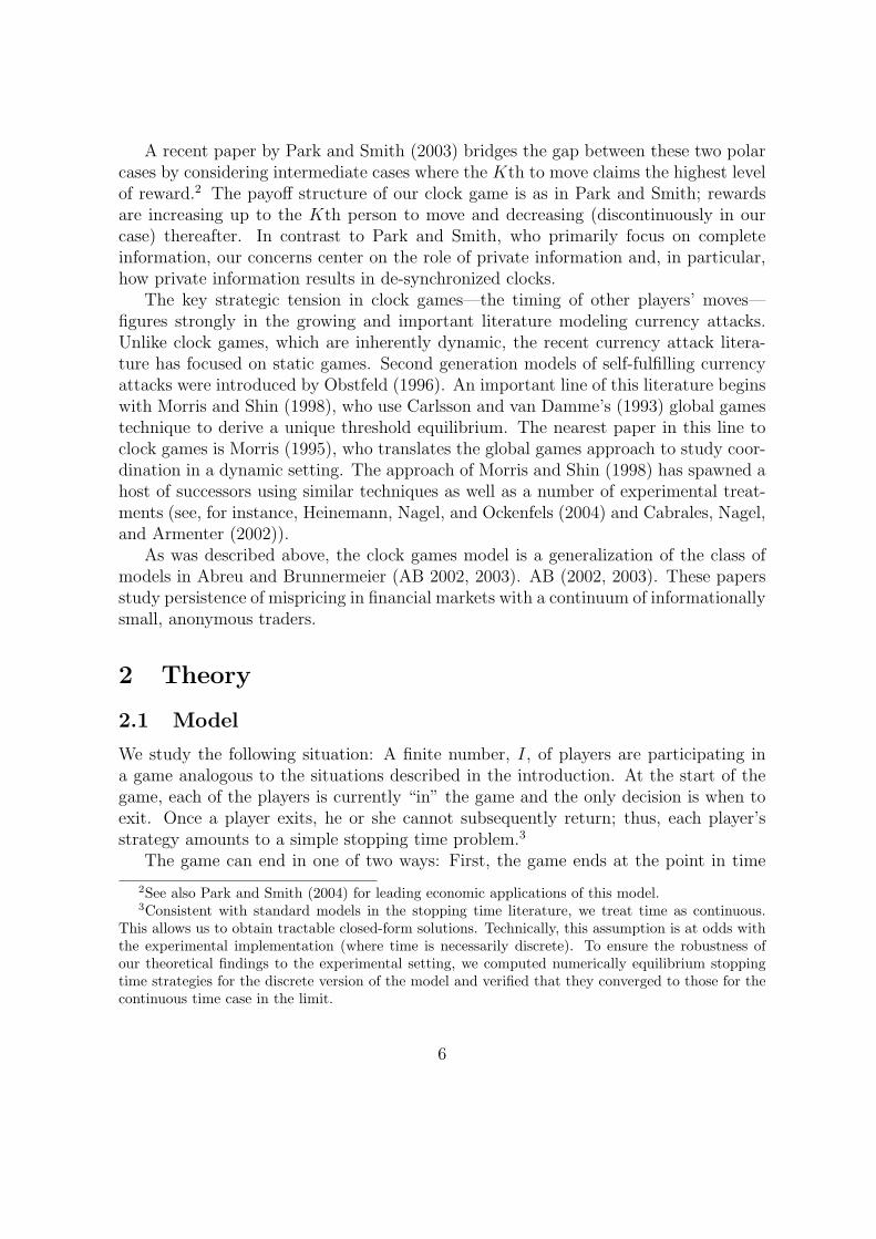
when a critical number, K < I, of the players have exited.4 Second, the game ends attime t0 + τ , where τ is commonly known, if fewer than K players exited by this point.A player’s payoff is determined by whether or not he exits before the game ends. If heexits before the game ends, at time t (say), then his “exit” payoff is egt. If, however,the game ends before the player exits, then he receives an “end-of-game” payoff, egt0 .The random variable t0 corresponds to the time in which the exit payoff starts toexceed the end-of-game payoff. We assume that t0 is exponentially distributed withp.d.f. f (t0) = λe−λt0 , where the constant λ is the arrival rate that t0 occurs in the nextinstant conditional on the event that it did not happen so far. Finally, if one playerexits exactly when the game ends, he still receives the exit payoff. If however moreplayers exit exactly at this point, we employ the following tie-breaking rule: Supposethat up to this point L < K players have exited. Then each of the remaining playershas an equal chance of obtaining one of the remaining K − L available “slots” andobtaining the exit payoff.

0

10

20

30

40

50

20 40 60 80 100 120 140 160 180 200 t

end of game

payoff

exit payoff

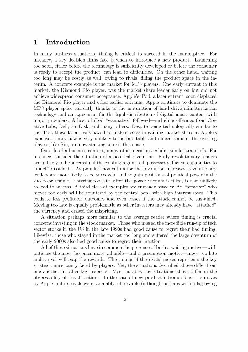
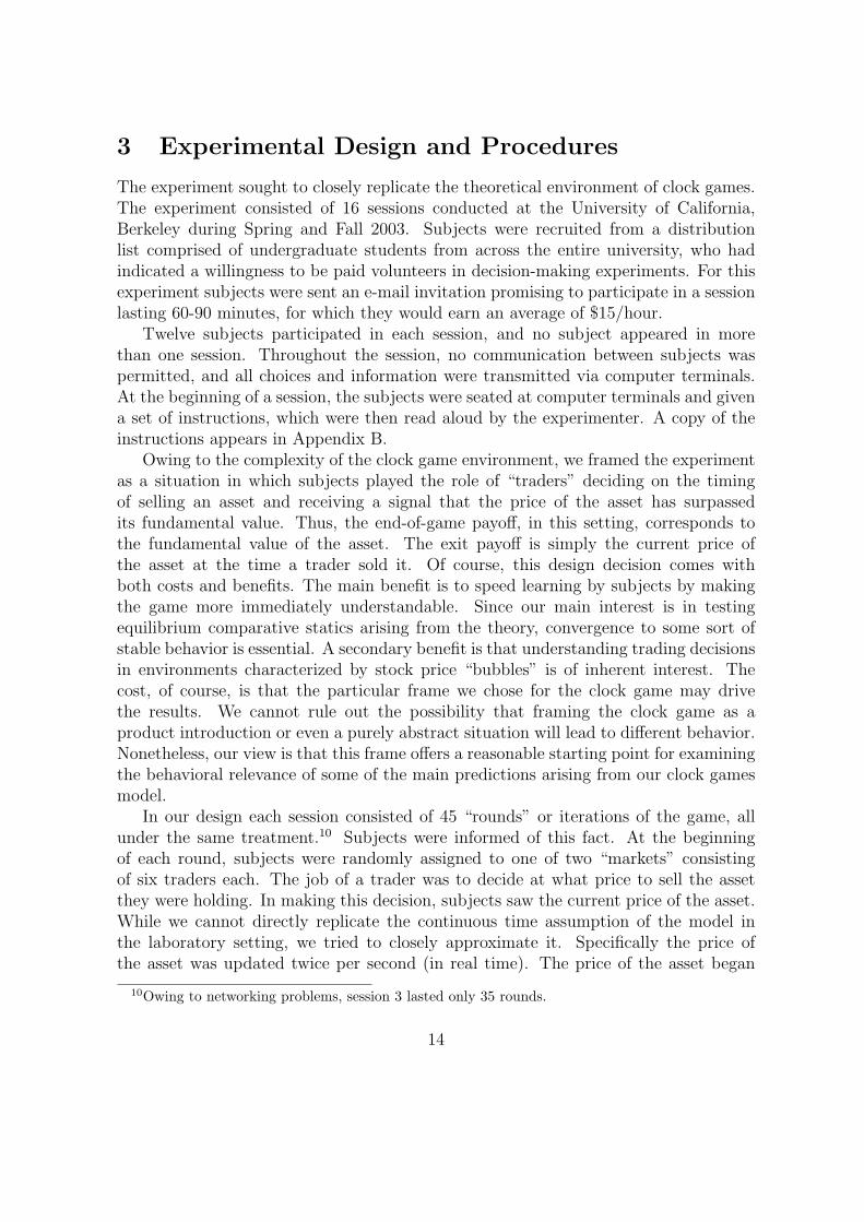
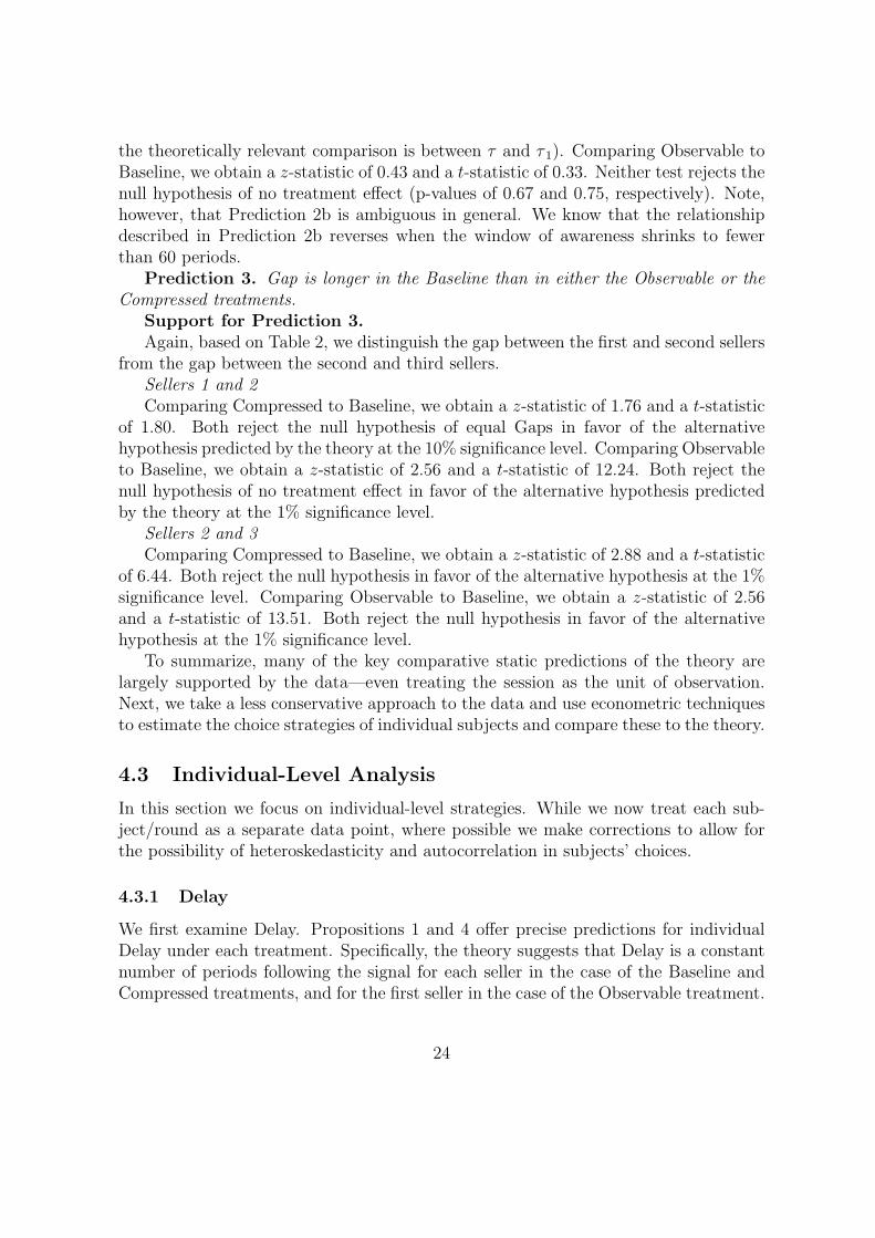
Figure 1: ‘Exit payoff’ versus ‘end of game payoff’

Interest in the model arises from the fact that a player can suffer drop in payoffby waiting too long to exit. That is, for any time beyond t0, a player’s end-of-gamepayoff is lower than his payoff if he exited at that moment since by waiting anotherinstant and exiting, the player enjoys growth rate g provided the game does not endin the interim. Figure 1 illustrates both types of payoffs for the case where t0 = 130

4As we explain in detail below, the game also ends if fewer than K players exit and the game hasbeen ongoing for a sufficiently long time.

7

and g = 2%. The payoffs from exiting (solid line) lie below the end-of-game payoffs(dotted line) for t < t0 and above for t > t0.

At time ti ≥ t0, player i receives a signal indicating that the exit payoff exceedsthe end-of-game payoff. It is helpful to think of time ti as the point at which playeri’s clock starts. The timing of i’s signal is uniformly distributed within the “windowof awareness” [t0, t0 + η], where η is the length of the window. That is, each playerdoes not exactly know when others received their signals. For instance, player i, whoreceives a signal at time ti, only knows at time ti + η that all other players receivedsignals. In Figure 1 the shaded rectangle illustrates the window of awareness for thecase where η = 50.

For the model to be interesting, the following assumptions are sufficient: (i) 0 <λ < g, (ii) τ large and (iii) η not too large. Assumption (i) guarantees that there issufficient upside to waiting, and so strategic delay becomes a possibility. Assumption(ii) ensures that the prospect of the game ending for exogenous reasons is not a strategicconsideration. Finally, assumption (iii) is needed to prevent the possible lag in the timea player receives a signal from becoming too large. Were this assumption violated, thenthe risk of a drop in payoff prior to receiving a signal would be sufficiently large thatplayers would always choose to exit prior to receiving the signal. Assumption (iii)may be stated more precisely as follows: Let η solve F (K, I, ηλ) = Ig

Ig−(I−K+1)λ, where

the function F (a, b, x) is a Kummer hypergeometric function (see e.g. Slater (1974)).5

From the monotonicity properties of F (·), such a solution always exists and is unique.Assumption (iii) requires that 0 < η < η.

While the model seeks to capture the central features shared by the situationsdescribed in the introduction where both waiting and preemptive motives are presentand where strategic uncertainty about the timing of a rival’s move is critical, it abstractsaway from detailed features unique to each situation. For instance, we do not modela change in the profit path of new product introductions as a function of the timingof past introductions other than to allow for a discontinuity in prices once the Kthentry occurs. Moreover, continuous effort in the form of the quality of the new productoffering, the financial size of the currency attack, nor the size of the revolutionaryorganization are modeled. Instead, we view our model as a basic model useful fordeveloping implications that are testable in the lab and as providing a kind of baselinemodel which might be enhanced for detailed study of any of the situations describedin the introduction.

Next, we characterize symmetric perfect Bayesian equilibria for two cases of the

5Many of the solutions to the model involve integral terms of the form

F (a, b, x) =(b− 1)!

(b− a− 1)! (a− 1)!

∫ 1

0

exzza−1 (1− z)b−a−1dz.

In the appendix, we describe some useful properties of Kummer functions.

8

model. In the unobservable actions case, the only information a player has is hersignal. In the observable actions case, in addition to her signal, each player learns ofthe exit of any other player. Formally, if player i exits at time t, then all other playersobserve this event at time limδ→0 (t + δ).

2.2 Unobservable Actions

Since all of the players in the game are ex ante identical, we restrict attention tosymmetric equilibria. In Proposition 1 we show that there is a unique symmetricequilibrium in our game. In this equilibrium, each player waits exactly τ periods afterreceiving his or her signal before exiting the game and exits immediately thereafter.We present a heuristic proof to illustrate the construction of this equilibrium below.6

In the Appendix, we formally establish both existence and uniqueness.First, fix the strategies of all other players as described above and consider the

problem faced by player i at time ti + τ . Player i faces an endogenous hazard rate,h, associated with the chance that the game will end in the next instant. For playeri to decide to exit the game at time ti + τ rather than to stay in, it must be the casethat player i’s expected profit from exiting at ti + τ is more than the expected profitfrom exiting at ti + τ + ∆. For small ∆, we can focus on the linear approximationof i’s payoffs ignoring the tie-breaking rule. Thus, the change in expected profit fromdelaying an additional ∆ periods is

(1− h∆) geg(ti+τ)∆− h∆E[eg(ti+τ) − egt0|D∆, ti

].

With a probability of approximately (1− h∆) the payoff increases at a rate of g. Notethat the expectations are taken conditional on the fact that the game will end in thenext ∆ interval (D∆) and on the time when i received the signal (ti). With probabilityof (approximately) h∆ the payoff drops (i.e., the game ends) within ti+τ and ti+τ +∆and exiting at ti + τ leads to the higher exit payoff eg(ti+τ) rather than the end-of-gamepayoff egt0 . Letting ∆ go to zero, the second order ∆2-terms vanish and, the optimalstopping time equates the marginal (log) benefits of delaying exiting with marginal(log) costs. That is,

hE[1− e−g(ti+τ−t0)|D0, ti

]= g. (1)

Note that[1− e−g(ti+τ−t0)

]is the drop in payoff as a fraction of the current payoff

eg(ti+τ). Solving for τ in equation (1) yields the optimal stopping time for player i

τ =1

g

[ln

h

h− g+ ln E

[e−g(ti−t0)|D0, ti

]]. (2)

Of course, equation (2) depends on the hazard rate, h, as well as on the conditionalexpectation E

[e−g(ti−t0)|D0, ti

]. Both expressions are determined in equilibrium.

6The proof is heuristic because we restrict attention to local deviations.

9

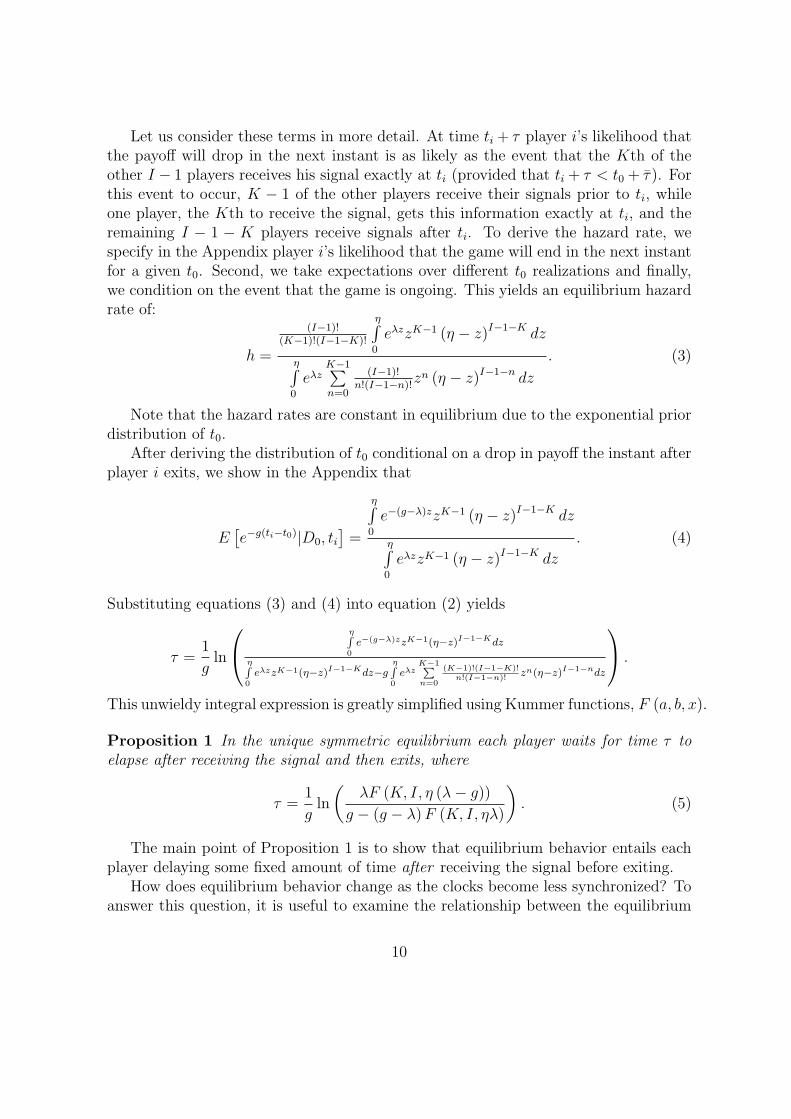
Let us consider these terms in more detail. At time ti + τ player i’s likelihood thatthe payoff will drop in the next instant is as likely as the event that the Kth of theother I − 1 players receives his signal exactly at ti (provided that ti + τ < t0 + τ). Forthis event to occur, K − 1 of the other players receive their signals prior to ti, whileone player, the Kth to receive the signal, gets this information exactly at ti, and theremaining I − 1 − K players receive signals after ti. To derive the hazard rate, wespecify in the Appendix player i’s likelihood that the game will end in the next instantfor a given t0. Second, we take expectations over different t0 realizations and finally,we condition on the event that the game is ongoing. This yields an equilibrium hazardrate of:

h =

(I−1)!(K−1)!(I−1−K)!

η∫0

eλzzK−1 (η − z)I−1−K dz

η∫0

eλzK−1∑n=0

(I−1)!n!(I−1−n)!

zn (η − z)I−1−n dz

. (3)

Note that the hazard rates are constant in equilibrium due to the exponential priordistribution of t0.

After deriving the distribution of t0 conditional on a drop in payoff the instant afterplayer i exits, we show in the Appendix that

E[e−g(ti−t0)|D0, ti

]=

η∫0

e−(g−λ)zzK−1 (η − z)I−1−K dz

η∫0

eλzzK−1 (η − z)I−1−K dz

. (4)

Substituting equations (3) and (4) into equation (2) yields

τ =1

gln

ηR0

e−(g−λ)zzK−1(η−z)I−1−Kdz

ηR0

eλzzK−1(η−z)I−1−Kdz−gηR0

eλzK−1Pn=0

(K−1)!(I−1−K)!n!(I−1−n)!

zn(η−z)I−1−ndz

.

This unwieldy integral expression is greatly simplified using Kummer functions, F (a, b, x).

Proposition 1 In the unique symmetric equilibrium each player waits for time τ toelapse after receiving the signal and then exits, where

τ =1

gln

(λF (K, I, η (λ− g))

g − (g − λ) F (K, I, ηλ)

). (5)

The main point of Proposition 1 is to show that equilibrium behavior entails eachplayer delaying some fixed amount of time after receiving the signal before exiting.

How does equilibrium behavior change as the clocks become less synchronized? Toanswer this question, it is useful to examine the relationship between the equilibrium

10

20

40

60

80

100

120

140

60 80 100 120

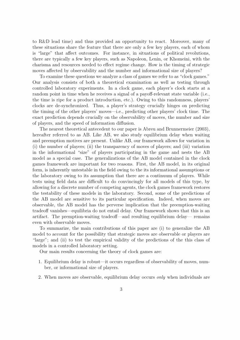
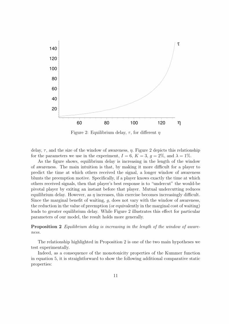
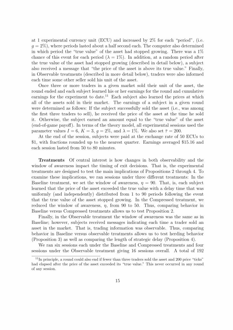
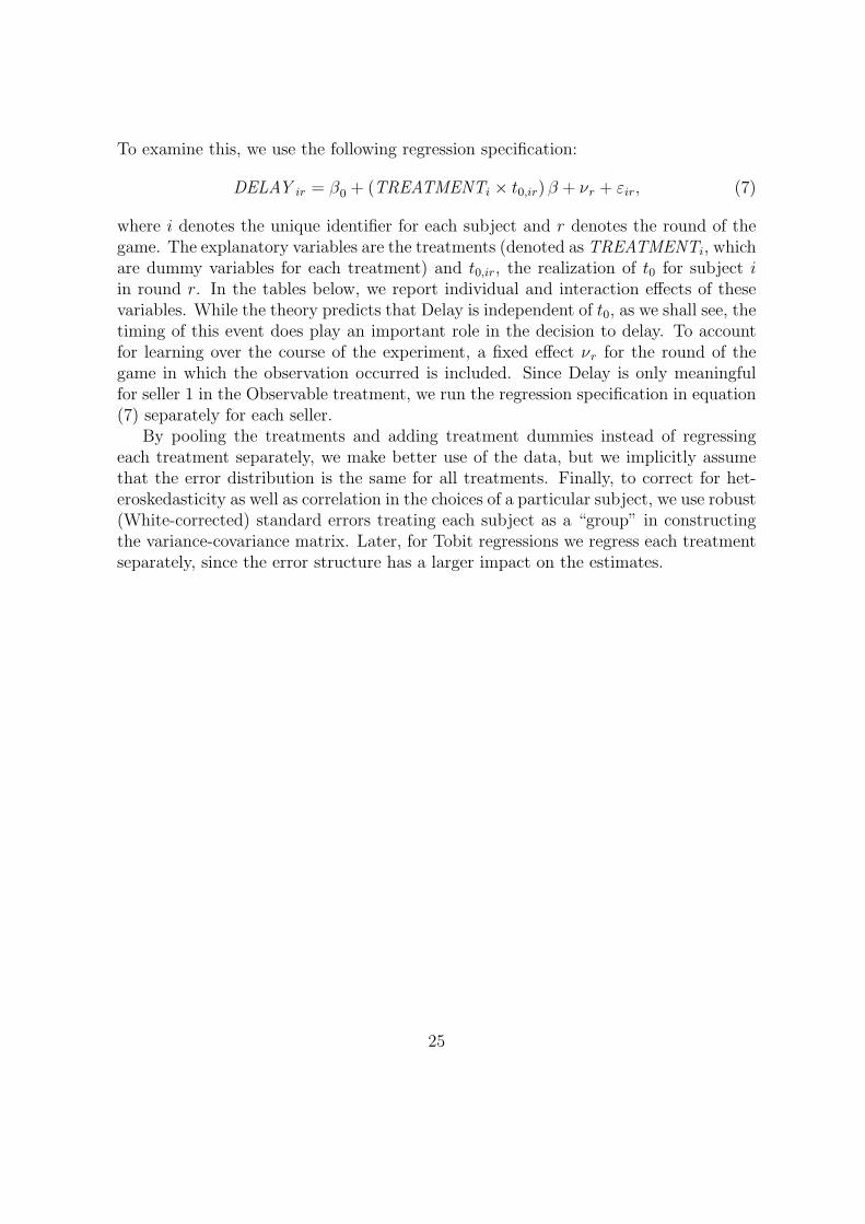
Figure 2: Equilibrium delay, τ , for different η

delay, τ , and the size of the window of awareness, η. Figure 2 depicts this relationshipfor the parameters we use in the experiment, I = 6, K = 3, g = 2%, and λ = 1%.

As the figure shows, equilibrium delay is increasing in the length of the windowof awareness. The main intuition is that, by making it more difficult for a player topredict the time at which others received the signal, a longer window of awarenessblunts the preemption motive. Specifically, if a player knows exactly the time at whichothers received signals, then that player’s best response is to “undercut” the would-bepivotal player by exiting an instant before that player. Mutual undercutting reducesequilibrium delay. However, as η increases, this exercise becomes increasingly difficult.Since the marginal benefit of waiting, g, does not vary with the window of awareness,the reduction in the value of preemption (or equivalently in the marginal cost of waiting)leads to greater equilibrium delay. While Figure 2 illustrates this effect for particularparameters of our model, the result holds more generally.

Proposition 2 Equilibrium delay is increasing in the length of the window of aware-ness.

The relationship highlighted in Proposition 2 is one of the two main hypotheses wetest experimentally.

Indeed, as a consequence of the monotonicity properties of the Kummer functionin equation 5, it is straightforward to show the following additional comparative staticproperties:

11

1. Equilibrium delay is increasing in K, the number of “exit slots.”

2. Equilibrium delay is decreasing in the I, the number of players.

2.3 Observable Actions

We saw above that in clock games where moves are unobservable, equilibrium behaviorentails delaying a fixed amount of time after receiving the signal before exiting. How-ever, in many situations of economic interest, players are able to observe each other’sactions. We now explore how observability affects strategic delay.

The following observation is crucial: Suppose that there is an equilibrium where,prior to anyone exiting, players exit only after having received the signal, then onobserving the first exit, the maximum time that can elapse before the game endsbecomes common knowledge for the remaining players.7 Thus, if the first exit occursat time t1, then it is common knowledge that the game will end no later than at timet1 + τ . Intuitively, the presence of a commonly known finite ending time to the gamenow allows one to apply backward induction in an analogous fashion to a number ofother timing games.8 A straightforward implication of this observation is the following:9

Proposition 3 In any perfect Bayesian equilibrium where the first player exits τ 1 pe-riods after receiving the signal, all other players exit immediately upon observing thisevent.

A key testable implication of Proposition 3 is that equilibrium behavior will neces-sarily give rise to herding following the decision of the first player to exit.

Of course, the model where exit is totally unobservable and the present situation,where exit is perfectly observable, represent the two extreme cases. Realistic situationswill tend to lie somewhere between these two. Together, Propositions 1 and 3 suggestthat the greater the observability of the exit decision, the more bunched are the exittimes.

Next, we turn to the timing of the exit decision prior to the first exit. To derivethe equilibrium delay, τ 1, let us again consider player i at time ti + τ 1. If he delaysexiting by an additional ∆ interval, he gains approximately geg(ti+τ1)∆ if the gamedoes not end. This event occurs with probability approximately 1 − ∆h1, where h1

7We make the usual assumption that all players’ conjectures about equilibrium strategies arecommonly known.

8Herding, in this instance, arises from the fact that the private information of the first player toexit is (partially) revealed by his decision to exit. This is analogous to the signaling role of the timingof moves which is prominent in Chamley and Gale (1994) as well as Gul and Lundholm (1995).

9While the argument above constitutes a proof for the discrete time case, our continuous timemodeling raises technical issues in applying backward induction. We offer a formal proof of Proposition3 in the Appendix.

12

is the endogenous hazard rate that some other player exits in the next instant. FromProposition 3, we know that, in this event, all remaining players will exit immediatelyin the subsequent instant. Following our tie-breaking rule, each exiting player has equalchance K−1

I−1of receiving the exit payoff (1 + g∆) eg(ti+τ1). Otherwise, a player receives

only the end-of-game payoff, egt0 . This yields the first-order condition:

(1−∆h1) geg(ti+τ1)∆+∆h1

{K − 1

I − 1geg(ti+τ1)∆− I −K

I − 1E

[eg(ti+τ1) − egt0|D∆, ti

]}= 0.

As ∆ goes to zero, the second order ∆2-terms vanish, and the first-order conditionsimplifies to

τ 1 =1

g

[ln

h1

h1 − g I−1I−K

+ ln E[e−g(ti−t0)|D0, ti

]]

. (6)

Comparing equation (6) with equation (2), the analogous expression when actionsare unobservable, one notices two key differences: First, g is replaced by I−1

I−Kg in the

first log-term in equation (2). This reflects the fact that, even after the first playerexits, all remaining players have a (K − 1) to (I − 1) chance of getting out at the highpayoff in the next instant. Second, the hazard rate of a drop in payoff is equal tothe conditional probability that the first player will exit in the next instant. In otherwords, the hazard rate is identical to that given in equation (3) if one sets K = 1.Finally, note that the term E

[e−g(ti−t0)|D0, ti

]is the same for both settings. Using

steps analogous to those leading to Proposition 1 allows us to derive τ 1 in closed formand thereby characterize a unique symmetric equilibrium to the game.

Proposition 4 In the unique symmetric equilibrium, if no players have exited, eachplayer waits for time τ 1 > 0 to elapse after receiving the signal and then exits, where

τ 1 =1

gln

(λF (1,I,η(−g+λ))

IgI−K+1

−( IgI−K+1

−λ)F (1,I,ηλ)

).

Once any player has exited, all other players exit immediately.

Proposition 4 has in common with Proposition 1 the feature that it is optimal fora player to delay exiting for a period of time after receiving the signal. Indeed, someproperties associated with equilibrium comparative statics for the unobservable casecontinue to hold in the observable case. For instance, following the same steps as in theproof of Proposition 2, one can readily show that equilibrium delay (τ 1) is increasingin the length of the window of awareness for the observable case as well.

How do the equilibrium delay times compare in the observable versus unobservablecases? In general, the effect is ambiguous. To see this, fix the parameter values of themodel at I = 6, K = 3, g = 2%, and λ = 1%. Numerical calculations show that τ 1 > τfor η < 59.8360 and τ 1 < τ for η > 59.8361. Thus, while strategic delay is common toboth cases, there is no systematic ordering between τ 1 and τ .

13

3 Experimental Design and Procedures

The experiment sought to closely replicate the theoretical environment of clock games.The experiment consisted of 16 sessions conducted at the University of California,Berkeley during Spring and Fall 2003. Subjects were recruited from a distributionlist comprised of undergraduate students from across the entire university, who hadindicated a willingness to be paid volunteers in decision-making experiments. For thisexperiment subjects were sent an e-mail invitation promising to participate in a sessionlasting 60-90 minutes, for which they would earn an average of $15/hour.

Twelve subjects participated in each session, and no subject appeared in morethan one session. Throughout the session, no communication between subjects waspermitted, and all choices and information were transmitted via computer terminals.At the beginning of a session, the subjects were seated at computer terminals and givena set of instructions, which were then read aloud by the experimenter. A copy of theinstructions appears in Appendix B.

Owing to the complexity of the clock game environment, we framed the experimentas a situation in which subjects played the role of “traders” deciding on the timingof selling an asset and receiving a signal that the price of the asset has surpassedits fundamental value. Thus, the end-of-game payoff, in this setting, corresponds tothe fundamental value of the asset. The exit payoff is simply the current price ofthe asset at the time a trader sold it. Of course, this design decision comes withboth costs and benefits. The main benefit is to speed learning by subjects by makingthe game more immediately understandable. Since our main interest is in testingequilibrium comparative statics arising from the theory, convergence to some sort ofstable behavior is essential. A secondary benefit is that understanding trading decisionsin environments characterized by stock price “bubbles” is of inherent interest. Thecost, of course, is that the particular frame we chose for the clock game may drivethe results. We cannot rule out the possibility that framing the clock game as aproduct introduction or even a purely abstract situation will lead to different behavior.Nonetheless, our view is that this frame offers a reasonable starting point for examiningthe behavioral relevance of some of the main predictions arising from our clock gamesmodel.

In our design each session consisted of 45 “rounds” or iterations of the game, allunder the same treatment.10 Subjects were informed of this fact. At the beginningof each round, subjects were randomly assigned to one of two “markets” consistingof six traders each. The job of a trader was to decide at what price to sell the assetthey were holding. In making this decision, subjects saw the current price of the asset.While we cannot directly replicate the continuous time assumption of the model inthe laboratory setting, we tried to closely approximate it. Specifically the price ofthe asset was updated twice per second (in real time). The price of the asset began

10Owing to networking problems, session 3 lasted only 35 rounds.

14

at 1 experimental currency unit (ECU) and increased by 2% for each “period”, (i.e.g = 2%), where periods lasted about a half second each. The computer also determinedin which period the “true value” of the asset had stopped growing. There was a 1%chance of this event for each period (λ = 1%). In addition, at a random period afterthe true value of the asset had stopped growing (described in detail below), a subjectalso received a message that “the price of the asset is above its true value.” Finally,in Observable treatments (described in more detail below), traders were also informedeach time some other seller sold his unit of the asset.

Once three or more traders in a given market sold their unit of the asset, theround ended and each subject learned his or her earnings for the round and cumulativeearnings for the experiment to date.11 Each subject also learned the prices at whichall of the assets sold in their market. The earnings of a subject in a given roundwere determined as follows: If the subject successfully sold the asset (i.e., was amongthe first three traders to sell), he received the price of the asset at the time he soldit. Otherwise, the subject earned an amount equal to the “true value” of the asset(end-of-game payoff). In terms of the theory model, all experimental sessions used theparameter values I = 6, K = 3, g = 2%, and λ = 1%. We also set τ = 200.

At the end of the session, subjects were paid at the exchange rate of 50 ECUs to$1, with fractions rounded up to the nearest quarter. Earnings averaged $15.16 andeach session lasted from 50 to 80 minutes.

Treatments Of central interest is how changes in both observability and thewindow of awareness impact the timing of exit decisions. That is, the experimentaltreatments are designed to test the main implications of Propositions 2 through 4. Toexamine these implications, we ran sessions under three different treatments: In theBaseline treatment, we set the window of awareness, η = 90. That, is, each subjectlearned that the price of the asset exceeded the true value with a delay time that wasuniformly (and independently) distributed from 1 to 90 periods following the eventthat the true value of the asset stopped growing. In the Compressed treatment, wereduced the window of awareness, η, from 90 to 50. Thus, comparing behavior inBaseline versus Compressed treatments allows us to test Proposition 2.

Finally, in the Observable treatment the window of awareness was the same as inBaseline; however, subjects received messages indicating each time a trader sold anasset in the market. That is, trading information was observable. Thus, comparingbehavior in Baseline versus observable treatments allows us to test herding behavior(Proposition 3) as well as comparing the length of strategic delay (Proposition 4).

We ran six sessions each under the Baseline and Compressed treatments and foursessions under the Observable treatment giving 16 sessions overall. A total of 192

11In principle, a round could also end if fewer than three traders sold the asset and 200 price “ticks”had elapsed after the price of the asset exceeded its “true value.” This never occurred in any roundof any session.

15

subjects participated in these experiments.

Experimental Design Rationale A key consideration in the experimental de-sign was to minimize information “leakage” about trading behavior in the experiment.That is, we wanted to minimize the possibility that subjects might use various auditory“cues” in detecting trading behavior by other subjects in the Baseline and Compressedtreatments. Specifically, we were concerned that having the subjects click their mouseon the sell button in order to sell would enable other traders to detect selling by listen-ing for mouse clicks. To remedy this problem, our experimental design had subjectssell by hovering their mouse over the sell button.

This was very effective in minimizing information leakage. However it did occa-sionally lead to subjects making what appear to us to be selling “mistakes.” Manysubjects evolved the strategy of placing their mouse pointer close to the sell box sothat they could quickly sell, but occasionally, their mouse pointer would inadvertentlystray into the sell box resulting in an unintended sale. Many of these mistakes are fairlyobvious in the data in that the first sale would sometimes take place after extremelyfew periods has occurred after the start of the round. In the case of the Baseline andObservable treatments, we “cleaned” the data by eliminating observations where salesoccur within the first 10 periods after the start of the round. In the case of the Ob-servable treatment, we dropped a round entirely when the first sale occurred withinthe first 10 periods.

While the decision a subject faced in each round of the game—when to sell theasset—is relatively simple, the price and information generating process are somewhatcomplicated. Thus, we expected that subjects would require several rounds of “learningby doing” before converging to a strategy as to how to play the game. As a conse-quence, our design stressed repetition in a stationary environment (45 iterations of thesame treatment). We also tried to speed the learning process by giving subjects exten-sive feedback about the profitability of their decisions as well as a comparison groupconsisting of the profits of other traders in the same market. Finally, when a subjectsold the asset below its true value, the subject received a message that this was thecase in addition to his or her usual report about trading profits at the end of a round.

We observed considerable variability in subject choices in the early rounds of thegame, suggesting that subjects were still learning the game. Behavior displayed muchless variability in the last 25 rounds of each session. Since we are primarily interested inthe performance of the model in equilibrium and not in learning to play the equilibriumstrategy, we confine attention in the results section below to these periods.12

One worry we had about running 45 iterations was that the game would become,in effect, a repeated game for subjects. To counter this possibility, we randomly and

12This is not to say that the nature of learning behavior in clock games is uninteresting per se.However, given our concerns with equilibrium comparative static predictions of the theory model, wefeel that a careful study of subject learning in clock games is beyond the scope of the present paper.

16

anonymously rematched subjects into different groups after each round of the game.Further, we prohibited communication among subjects. Thus, while it is theoreti-cally possible for subjects to coordinate on dynamic trading strategies, achieving therequired coordination struck us as difficult. In examining the data, we looked for evi-dence of “collusive” strategies on the part of subjects. Such strategies might consist ofdelaying an excessively long time to sell after receiving the signal or coordinating on aparticular price of the asset at which to sell regardless of signals received. We foundno evidence of either type of behavior. Further, no subject mentioned coordinating ordynamic strategies in their responses to the post-experiment questionnaire. Thus, weare reasonably confident that subjects were, in fact, treating the game as a one-shotgame as described in the theory.

To get a sense of how well subjects understood the game at the end of a session, weasked each subject to fill out a post-experiment questionnaire where they were askedto describe their strategy. In the vast majority of instances, subjects described theirstrategies as waiting for the price of the asset to rise a certain amount after receivingthe message that the asset was above its true value and then selling.13

4 Results

In this section we present the results of the laboratory experiment. We are mainlyinterested in the following measures of subject choices:

1. Duration: We measure the length, in periods from t0 until the end of the game—that is, the period in which the third seller sold the asset. In the event that thegame ended in a period prior to t0, we code Duration as zero.

2. Delay: We measure the length, in periods, of strategic delay by sellers. Thevariable Delay for seller i is the number of periods between the time he receivedthe signal until the time he sold the asset. If i never sold the asset, then no Delayis assigned. If i sold at or before the time he received the signal, Delay equalszero.14

3. Gap: We measure the gap, in periods, between the sale times of the ith andi + 1th subjects selling the asset.

The first two measures, Duration and Delay, enable us to study the main implicationof Propositions 1 and 4—namely that equilibrium behavior will lead traders to engage

13The formal empirical analysis makes no use of the answers given in the questionnaire.14We also investigated an alternative coding scheme whereby a missing value was assigned for the

Delay of sellers who sold but never received the signal. The results are qualitatively unaffected bythis alternative. Details are available from the authors upon request.

17

in strategic delay. Indeed, the Delay measure is the empirical counterpart to the τ andτ 1 predictions derived in the theory. Further, the main implication of Proposition 2 isthat a reduction in the window of awareness reduces both Duration and Delay. Finally,the measure Gap seeks to capture the key behavioral prediction of Proposition 3—thatobservable trading information leads to “herding” on the part of sellers following thefirst sale.15 Table 1 presents the predictions of the theory model for each of theseperformance measures. The parameters chosen for each of the treatments were designedto generate large differences in the performance measures. In particular, as Table 1shows, the expected Duration is predicted to be longest in the Baseline treatmentand shortest in the Compressed and Observable treatments. Delay is predicted to bemuch shorter under the Compressed or Observable treatments compared to Baseline.Finally, the expectation of the Gap measure illustrates a distinct difference between theBaseline and Compressed treatments and the Observable treatment, which is predictedto have negligible gap length.

Table 1: Theory Predictions

TreatmentBaseline Compressed Observable

Duration 62 26 26Delay* 23 5 13Gap 13 7 1

* For the Observable treatment, Delay is only meaningful for the first seller.

4.1 Overview

Table 2 presents descriptive statistics from the experimental data for these same per-formance measures, treating each session as an independent observation. Beginningwith the Duration measure, notice that the ordering implied by the theory is mainlyreflected in the data: the longest average Duration occurs in the Baseline treatment,whereas the Observable and Compressed treatments exhibit shorter, but comparableDurations.

15One may worry that, since periods lasted about a half second each, a subject may have hadinsufficient time to react to the event of a sell by another subject with only a one period delay.However, most studies of reaction time to light stimuli for college age individuals indicate a meanreaction time of approximately 0.19 seconds. See, for instance Welford (1980).

18

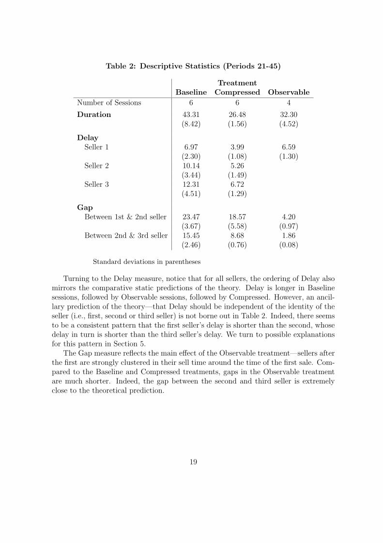
Table 2: Descriptive Statistics (Periods 21-45)

TreatmentBaseline Compressed Observable

Number of Sessions 6 6 4

Duration 43.31 26.48 32.30(8.42) (1.56) (4.52)

DelaySeller 1 6.97 3.99 6.59

(2.30) (1.08) (1.30)Seller 2 10.14 5.26

(3.44) (1.49)Seller 3 12.31 6.72

(4.51) (1.29)

GapBetween 1st & 2nd seller 23.47 18.57 4.20

(3.67) (5.58) (0.97)Between 2nd & 3rd seller 15.45 8.68 1.86

(2.46) (0.76) (0.08)

Standard deviations in parentheses

Turning to the Delay measure, notice that for all sellers, the ordering of Delay alsomirrors the comparative static predictions of the theory. Delay is longer in Baselinesessions, followed by Observable sessions, followed by Compressed. However, an ancil-lary prediction of the theory—that Delay should be independent of the identity of theseller (i.e., first, second or third seller) is not borne out in Table 2. Indeed, there seemsto be a consistent pattern that the first seller’s delay is shorter than the second, whosedelay in turn is shorter than the third seller’s delay. We turn to possible explanationsfor this pattern in Section 5.

The Gap measure reflects the main effect of the Observable treatment—sellers afterthe first are strongly clustered in their sell time around the time of the first sale. Com-pared to the Baseline and Compressed treatments, gaps in the Observable treatmentare much shorter. Indeed, the gap between the second and third seller is extremelyclose to the theoretical prediction.

19

0.0

5.1

.15

0.0

5.1

.15

0 50 100

0 50 100

Baseline Compressed

ObservableDen

sity

Duration in PeriodsGraphs by Treatment

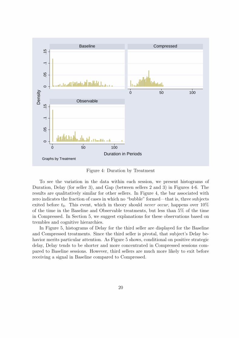
Figure 4: Duration by Treatment

To see the variation in the data within each session, we present histograms ofDuration, Delay (for seller 3), and Gap (between sellers 2 and 3) in Figures 4-6. Theresults are qualitatively similar for other sellers. In Figure 4, the bar associated withzero indicates the fraction of cases in which no “bubble” formed—that is, three subjectsexited before t0. This event, which in theory should never occur, happens over 10%of the time in the Baseline and Observable treatments, but less than 5% of the timein Compressed. In Section 5, we suggest explanations for these observations based ontrembles and cognitive hierarchies.

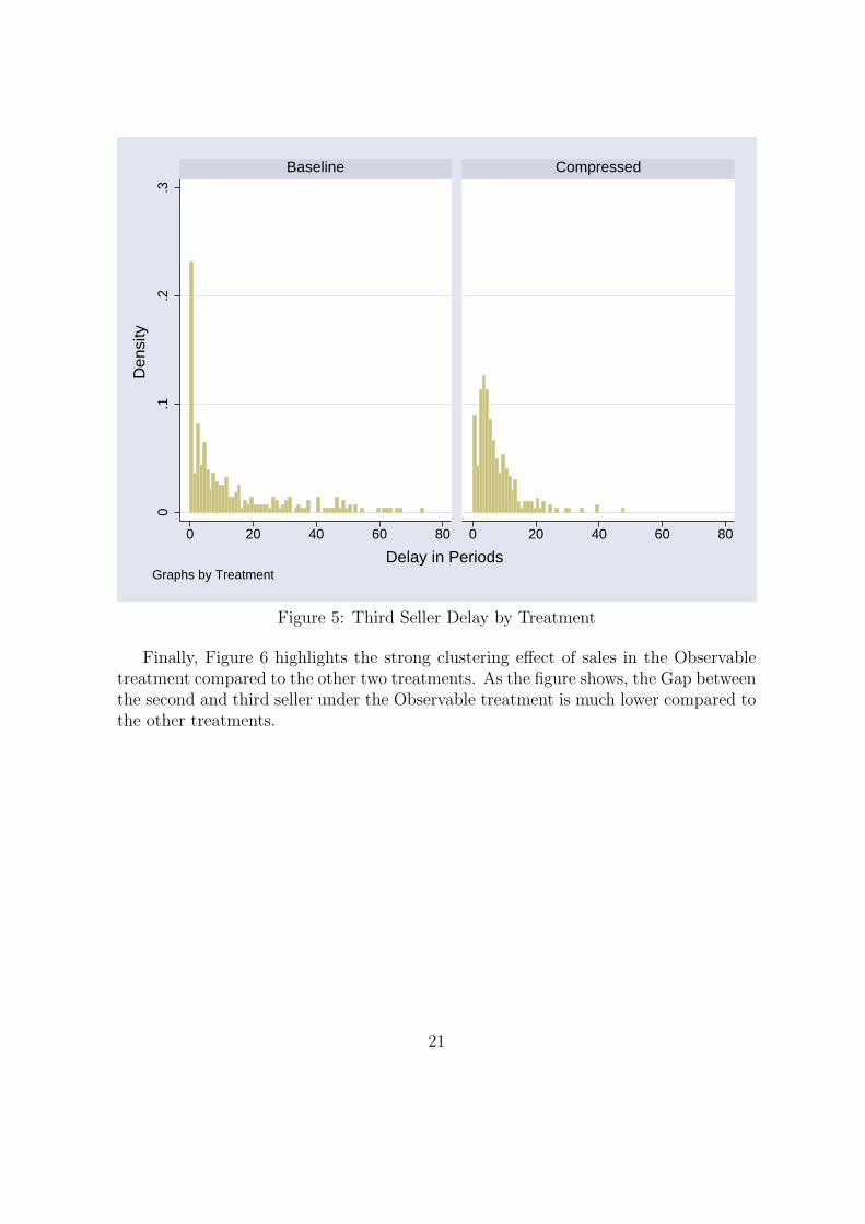
In Figure 5, histograms of Delay for the third seller are displayed for the Baselineand Compressed treatments. Since the third seller is pivotal, that subject’s Delay be-havior merits particular attention. As Figure 5 shows, conditional on positive strategicdelay, Delay tends to be shorter and more concentrated in Compressed sessions com-pared to Baseline sessions. However, third sellers are much more likely to exit beforereceiving a signal in Baseline compared to Compressed.

20

0.1

.2.3

0 20 40 60 80 0 20 40 60 80

Baseline Compressed

Den

sity

Delay in PeriodsGraphs by Treatment

Figure 5: Third Seller Delay by Treatment

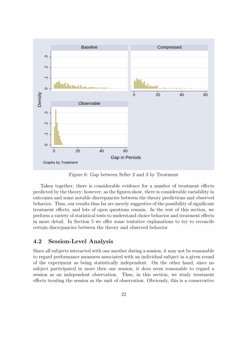
Finally, Figure 6 highlights the strong clustering effect of sales in the Observabletreatment compared to the other two treatments. As the figure shows, the Gap betweenthe second and third seller under the Observable treatment is much lower compared tothe other treatments.

21

0.1

.2.3

0.1

.2.3

0 20 40 60

0 20 40 60

Baseline Compressed

ObservableDen

sity

Gap in PeriodsGraphs by Treatment

Figure 6: Gap between Seller 2 and 3 by Treatment

Taken together, there is considerable evidence for a number of treatment effectspredicted by the theory; however, as the figures show, there is considerable variability inoutcomes and some notable discrepancies between the theory predictions and observedbehavior. Thus, our results thus far are merely suggestive of the possibility of significanttreatment effects, and lots of open questions remain. In the rest of this section, weperform a variety of statistical tests to understand choice behavior and treatment effectsin more detail. In Section 5 we offer some tentative explanations to try to reconcilecertain discrepancies between the theory and observed behavior

4.2 Session-Level Analysis

Since all subjects interacted with one another during a session, it may not be reasonableto regard performance measures associated with an individual subject in a given roundof the experiment as being statistically independent. On the other hand, since nosubject participated in more then one session, it does seem reasonable to regard asession as an independent observation. Thus, in this section, we study treatmenteffects treating the session as the unit of observation. Obviously, this is a conservative

22

approach to the data—it reduces the dataset to 16 observations—nonetheless, we beginwith this approach in assessing treatment effects. Throughout, we rely on two types ofstatistical tests to formally investigate treatment effects. The first test is a WilcoxonRank-Sum (or Mann-Whitney) test of equality of unmatched pairs of observations.This is a non-parametric test which gives back a z-statistic which may be used inhypothesis testing. Our second test is a standard t-test under the assumption of unequalvariances. This test has the advantage of familiarity, but the disadvantage of requiringadditional distributional assumptions on the data to be valid. As we will show belowthe conclusions drawn from the two tests rarely differ for our data.

Relying on Propositions 2 and 4 we test the following predictions.Prediction 1. Duration is longer in the Baseline than in either the Compressed

or the Observable treatments.Support for Prediction 1.We test the null hypothesis of no treatment effect against the one-sided alternative

predicted by the theory. Comparing Compressed to Baseline, we obtain a z-statistic of2.88 and a t-statistic of 4.81. Both reject the null hypothesis in favor of the alternativehypothesis at the 1% significance level. Comparing Observable to Baseline, we obtaina z-statistic of 1.92 and a t-statistic of 2.68. Both reject the null hypothesis in favor ofthe alternative hypothesis at the 5% significance level.

Prediction 2.a Delay is longer in the Baseline than in the Compressed treatment.Support for Prediction 2a.Since Table 2 suggested that the first, second, and third sellers behave somewhat

differently, we test the null hypothesis of no treatment effect against the one-sidedalternative implied by the theory separately for each seller.

Seller 1.Comparing Compressed to Baseline, we obtain a z-statistic of 2.08 and a t-statistic

of 2.87. Both reject the null hypothesis in favor of the alternative hypothesis at the5% significance level.

Seller 2.Comparing Compressed to Baseline, we obtain a z-statistic of 2.08 and a t-statistic

of 3.19. Both reject the null hypothesis in favor of the alternative hypothesis at the5% significance level.

Seller 3.Comparing Compressed to Baseline, we obtain a z-statistic of 2.08 and a t-statistic

of 2.92. Both reject the null hypothesis in favor of the alternative hypothesis at the5% significance level.

Taken together, these results provide strong support at the session level for Propo-sition 2.

Prediction 2b. Delay is longer in the Baseline than in the Observable treatment.Lack of Support for Prediction 2b.For the comparison to be meaningful, we restrict attention to the first seller (since

23

the theoretically relevant comparison is between τ and τ 1). Comparing Observable toBaseline, we obtain a z-statistic of 0.43 and a t-statistic of 0.33. Neither test rejects thenull hypothesis of no treatment effect (p-values of 0.67 and 0.75, respectively). Note,however, that Prediction 2b is ambiguous in general. We know that the relationshipdescribed in Prediction 2b reverses when the window of awareness shrinks to fewerthan 60 periods.

Prediction 3. Gap is longer in the Baseline than in either the Observable or theCompressed treatments.

Support for Prediction 3.Again, based on Table 2, we distinguish the gap between the first and second sellers

from the gap between the second and third sellers.Sellers 1 and 2Comparing Compressed to Baseline, we obtain a z-statistic of 1.76 and a t-statistic

of 1.80. Both reject the null hypothesis of equal Gaps in favor of the alternativehypothesis predicted by the theory at the 10% significance level. Comparing Observableto Baseline, we obtain a z-statistic of 2.56 and a t-statistic of 12.24. Both reject thenull hypothesis of no treatment effect in favor of the alternative hypothesis predictedby the theory at the 1% significance level.

Sellers 2 and 3Comparing Compressed to Baseline, we obtain a z-statistic of 2.88 and a t-statistic

of 6.44. Both reject the null hypothesis in favor of the alternative hypothesis at the 1%significance level. Comparing Observable to Baseline, we obtain a z-statistic of 2.56and a t-statistic of 13.51. Both reject the null hypothesis in favor of the alternativehypothesis at the 1% significance level.

To summarize, many of the key comparative static predictions of the theory arelargely supported by the data—even treating the session as the unit of observation.Next, we take a less conservative approach to the data and use econometric techniquesto estimate the choice strategies of individual subjects and compare these to the theory.

4.3 Individual-Level Analysis

In this section we focus on individual-level strategies. While we now treat each sub-ject/round as a separate data point, where possible we make corrections to allow forthe possibility of heteroskedasticity and autocorrelation in subjects’ choices.

4.3.1 Delay

We first examine Delay. Propositions 1 and 4 offer precise predictions for individualDelay under each treatment. Specifically, the theory suggests that Delay is a constantnumber of periods following the signal for each seller in the case of the Baseline andCompressed treatments, and for the first seller in the case of the Observable treatment.

24

To examine this, we use the following regression specification:

DELAY ir = β0 + (TREATMENTi × t0,ir) β + νr + εir, (7)

where i denotes the unique identifier for each subject and r denotes the round of thegame. The explanatory variables are the treatments (denoted as TREATMENTi, whichare dummy variables for each treatment) and t0,ir, the realization of t0 for subject iin round r. In the tables below, we report individual and interaction effects of thesevariables. While the theory predicts that Delay is independent of t0, as we shall see, thetiming of this event does play an important role in the decision to delay. To accountfor learning over the course of the experiment, a fixed effect νr for the round of thegame in which the observation occurred is included. Since Delay is only meaningfulfor seller 1 in the Observable treatment, we run the regression specification in equation(7) separately for each seller.

By pooling the treatments and adding treatment dummies instead of regressingeach treatment separately, we make better use of the data, but we implicitly assumethat the error distribution is the same for all treatments. Finally, to correct for het-eroskedasticity as well as correlation in the choices of a particular subject, we use robust(White-corrected) standard errors treating each subject as a “group” in constructingthe variance-covariance matrix. Later, for Tobit regressions we regress each treatmentseparately, since the error structure has a larger impact on the estimates.

25

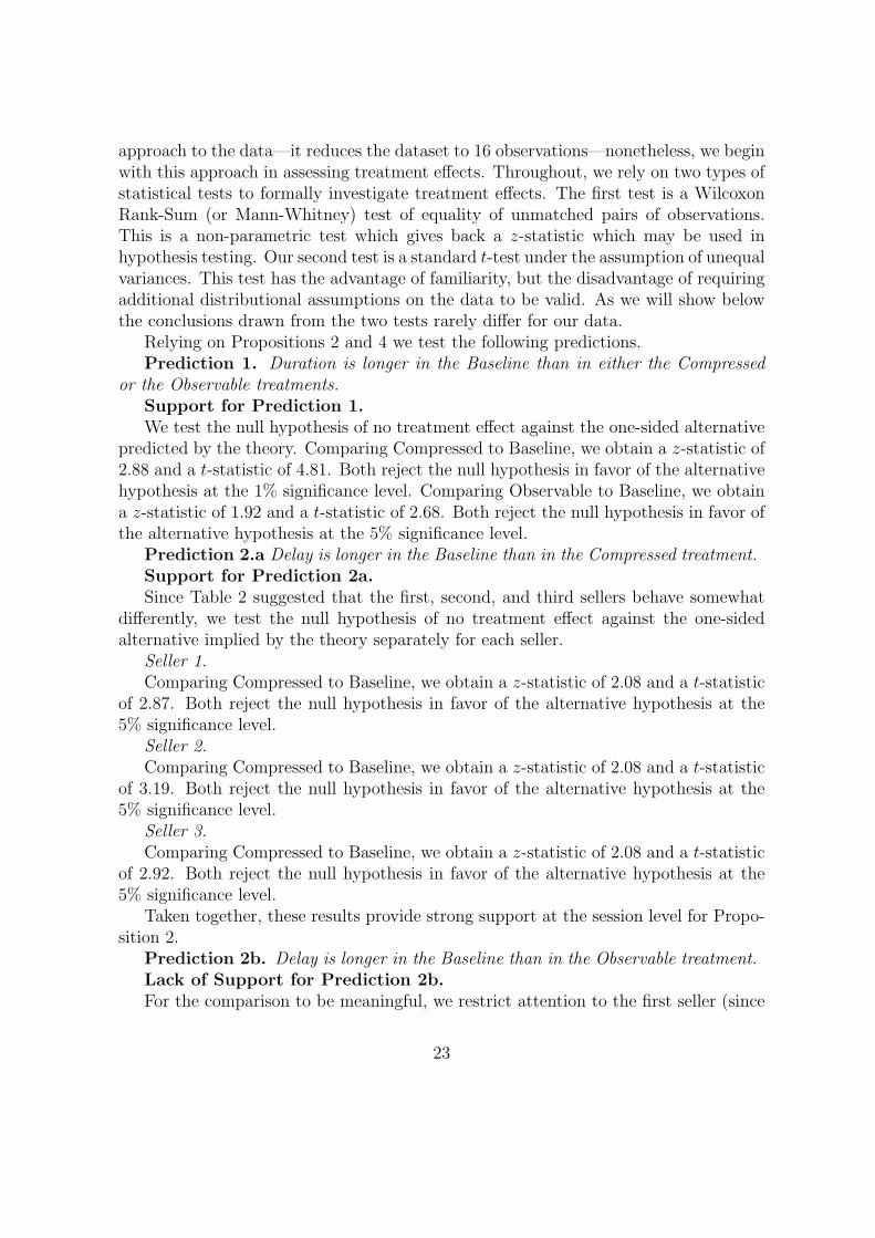
Table 3: Delay Estimates

Robust-Cluster-OLS TobitSeller 1 Seller 2 Seller 3 Baseline Compressed

Constant 12.841 17.931 22.803 17.277 11.011(10.78)∗∗ (10.30)∗∗ (10.28)∗∗ (5.31)∗∗ (7.46)∗∗

Compressed −6.861 −10.281 −13.023(5.16)∗∗ (5.22)∗∗ (5.17)∗∗

Observable −2.169(1.07)

t0 −0.071 −0.097 −0.127(9.59)∗∗ (8.17)∗∗ (8.81)∗∗

t0 × Compressed 0.045 0.064 0.086(5.03)∗∗ (4.59)∗∗ (4.82)∗∗

t0 × Observable 0.012(0.93)

Round Fixed Effects Yes Yes Yes Yes Yes

Observations 738 584 583 1681 1788R-squared 0.23 0.26 0.28

OLS: Robust t-statistics in parentheses. Tobit: Standard t-statistics in parentheses* significant at 5%; ** significant at 1%

OLS Regressions. The first column of Table 3 shows the results of this analysisrestricting attention to subjects who execute the first sale in each round of the ex-periment.16 The regression coefficient estimates imply that the Compressed treatmentreduces Delay by 3.48 periods, which is statistically different from zero at the 1% sig-nificance level (F -statistic 19.25), but far from the 18 period reduction predicted bythe theory.17 The regression coefficient estimates imply that the Observable treatmentreduces Delay by 1.27 periods, although this is statistically indistinguishable from zeroat conventional significance levels (F -statistic 1.14). These results are in the directionpredicted by the theory, but clearly inconsistent with the level predictions.

16In the event that multiple sellers sold in the same period and no sales were executed prior to thisperiod, we randomly assign one of these sellers the identity of “first” seller.

17Recall that the estimated mean marginal effect of the Compressed treatment is equal to theCompressed coefficient plus the coefficient of the interaction term times the sample mean of t0, whichwas approximately equal to 75 in the dataset.

26

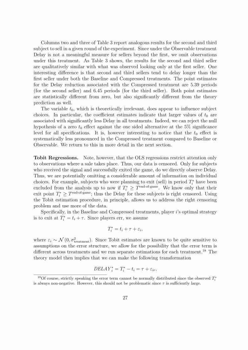
Columns two and three of Table 3 report analogous results for the second and thirdsubject to sell in a given round of the experiment. Since under the Observable treatmentDelay is not a meaningful measure for sellers beyond the first, we omit observationsunder this treatment. As Table 3 shows, the results for the second and third sellerare qualitatively similar with what was observed looking only at the first seller. Oneinteresting difference is that second and third sellers tend to delay longer than thefirst seller under both the Baseline and Compressed treatments. The point estimatesfor the Delay reduction associated with the Compressed treatment are 5.39 periods(for the second seller) and 6.45 periods (for the third seller). Both point estimatesare statistically different from zero, but also significantly different from the theoryprediction as well.

The variable t0, which is theoretically irrelevant, does appear to influence subjectchoices. In particular, the coefficient estimates indicate that larger values of t0 areassociated with significantly less Delay in all treatments. Indeed, we can reject the nullhypothesis of a zero t0 effect against the one sided alternative at the 5% significancelevel for all specifications. It is, however interesting to notice that the t0 effect issystematically less pronounced in the Compressed treatment compared to Baseline orObservable. We return to this in more detail in the next section.

Tobit Regressions. Note, however, that the OLS regressions restrict attention onlyto observations where a sale takes place. Thus, our data is censored. Only for subjectswho received the signal and successfully exited the game, do we directly observe Delay.Thus, we are potentially omitting a considerable amount of information on individualchoices. For example, subjects who were planning to exit (sell) in period T ∗

i have beenexcluded from the analysis up to now if T ∗

i ≥ T end-of-game. We know only that theirexit point T ∗

i ≥ T end-of-game; thus the Delay for these subjects is right censored. Usingthe Tobit estimation procedure, in principle, allows us to address the right censoringproblem and use more of the data.

Specifically, in the Baseline and Compressed treatments, player i’s optimal strategyis to exit at T ∗

i = ti + τ . Since players err, we assume

T ∗i = ti + τ + εi,

where εi ∼ N (0, σ2treatment). Since Tobit estimates are known to be quite sensitive to

assumptions on the error structure, we allow for the possibility that the error term isdifferent across treatments and we run separate estimations for each treatment.18 Thetheory model then implies that we can make the following transformation

DELAY ∗i = T ∗

i − ti = τ + εir,

18Of course, strictly speaking the error term cannot be normally distributed since the observed T ∗iis always non-negative. However, this should not be problematic since τ is sufficiently large.

27

where DELAY ∗i |ti ∼ N (τ , σ2

treatment). Using this transformation, we are now in a po-sition to use the Tobit procedure to obtain estimates of Delay under the Baseline andCompressed treatments.19 These estimates are reported in columns 4 and 5 of Table3. Notice that the estimated Delay for the Baseline treatment (17.277) is considerablyhigher than the Delays for sellers 1 through 3 shown in Table 2.

Turning to the Compressed treatment, notice that the estimated Delay is consid-erably lower (11.011) than under the Baseline treatment as predicted by the theory.Formally, one can easily reject the null hypothesis that the parameter estimate for De-lay length are equal at the 1% significance level. In contrast to Baseline, the estimatedDelay under the Compressed treatment is larger than the theory prediction (Delay =5), and one can reject the null hypothesis implied by the theory against the two-sidedalternative at the 1% significance level.

To summarize, it is reassuring that the two main predictions of the theory—thatthere is significant strategic delay and that delay is increasing in the length of the win-dow of awareness are borne out in both the OLS and Tobit estimates. That being said,a key difficulty with the Tobit estimation procedure is that it (of necessity) excludesfactors such as the time that the true value of the asset stopped growing (t0) as well asround fixed effects that we know, from the OLS regressions, do affect subject choices.Thus, our view is the main value of this analysis is in capturing qualitative treatmenteffects rather than in generating exact point estimates. Indeed, taken as a whole, Table3 shows that point estimates of Delay can vary a good deal depending on the sampleand estimation procedure employed.

4.3.2 Herding Behavior

Next, we turn to estimates of herding behavior by subjects. In the beginning of thissection we introduced the measure GAP kl, which measures the number of periodsbetween the sale times of the lth seller and the kth seller. Recall that the theorypredicts that Gap is shorter for the Compressed than for the Baseline treatment. Forthe Observable treatment, the theory predicts zero Gaps. Note however that, owing tothe discretization of time in the experimental implementation of the theory, informationabout time of the first sale is delayed by about a half second (one period); hence, thetheory effectively implies that GAP 12 = 1 and GAP 23 = 0 in the Observable treatment.To examine this, we run the following regression:

GAPklir = β (TREATMENTi × t0,ir) + νr + εir, (8)

where the variables are defined as in equation (7).

19As for the case with the second and third sellers in the OLS regressions, the analysis is notmeaningful in the case of the Observable treatment.

28

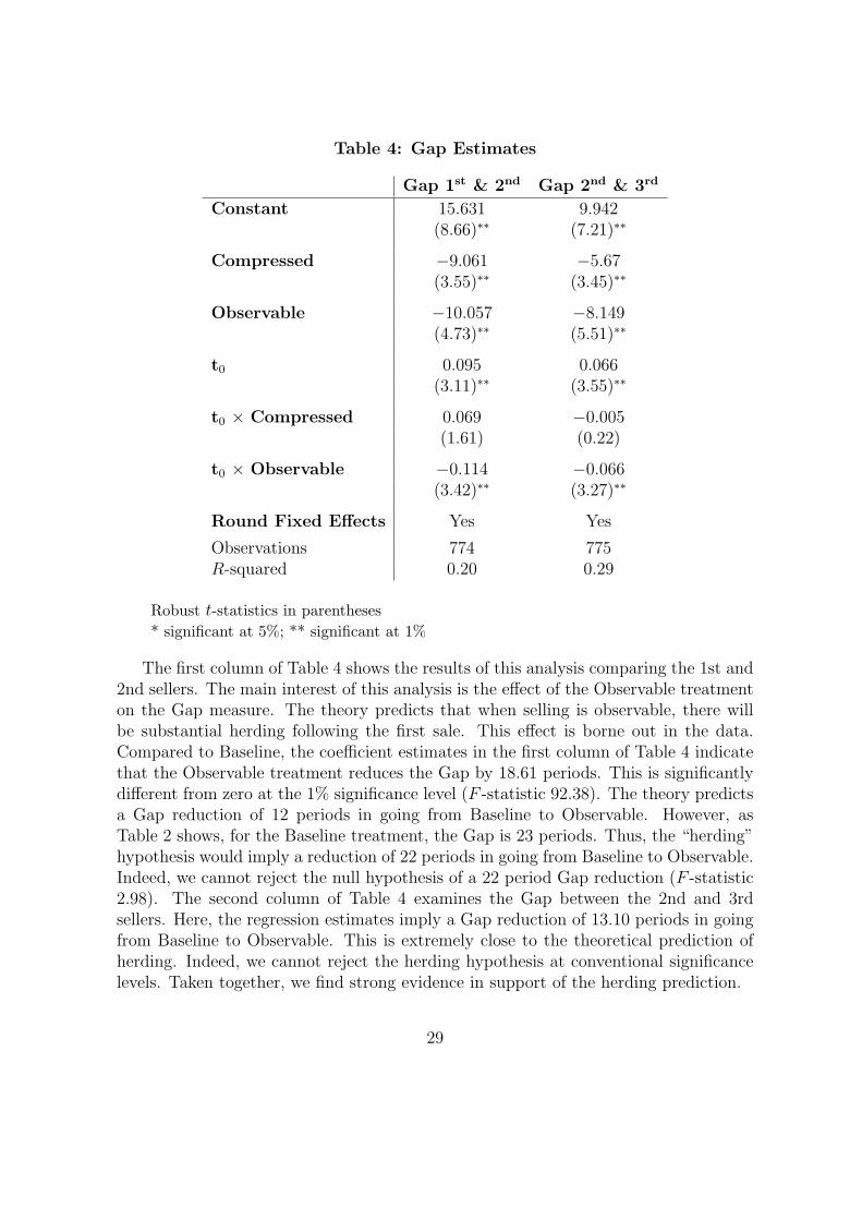
Table 4: Gap Estimates

Gap 1st & 2nd Gap 2nd & 3rd

Constant 15.631 9.942(8.66)∗∗ (7.21)∗∗

Compressed −9.061 −5.67(3.55)∗∗ (3.45)∗∗

Observable −10.057 −8.149(4.73)∗∗ (5.51)∗∗

t0 0.095 0.066(3.11)∗∗ (3.55)∗∗

t0 × Compressed 0.069 −0.005(1.61) (0.22)

t0 × Observable −0.114 −0.066(3.42)∗∗ (3.27)∗∗

Round Fixed Effects Yes Yes

Observations 774 775R-squared 0.20 0.29

Robust t-statistics in parentheses* significant at 5%; ** significant at 1%

The first column of Table 4 shows the results of this analysis comparing the 1st and2nd sellers. The main interest of this analysis is the effect of the Observable treatmenton the Gap measure. The theory predicts that when selling is observable, there willbe substantial herding following the first sale. This effect is borne out in the data.Compared to Baseline, the coefficient estimates in the first column of Table 4 indicatethat the Observable treatment reduces the Gap by 18.61 periods. This is significantlydifferent from zero at the 1% significance level (F -statistic 92.38). The theory predictsa Gap reduction of 12 periods in going from Baseline to Observable. However, asTable 2 shows, for the Baseline treatment, the Gap is 23 periods. Thus, the “herding”hypothesis would imply a reduction of 22 periods in going from Baseline to Observable.Indeed, we cannot reject the null hypothesis of a 22 period Gap reduction (F -statistic2.98). The second column of Table 4 examines the Gap between the 2nd and 3rdsellers. Here, the regression estimates imply a Gap reduction of 13.10 periods in goingfrom Baseline to Observable. This is extremely close to the theoretical prediction ofherding. Indeed, we cannot reject the herding hypothesis at conventional significancelevels. Taken together, we find strong evidence in support of the herding prediction.

29

Next, turning to the Compressed treatment, notice that the regression estimates incolumn 1 of Table 4 imply a 3.88 period reduction in the Gap between the 1st and 2ndsellers in going from Baseline to Compressed. While this is in the direction predicted bythe theory, we cannot reject the null hypothesis of no treatment effect at conventionalsignificance levels (F -statistic 2.40). The second column of Table 4 shows that theGap between the 2nd and 3rd sellers is reduced by 6.05 periods in going from Baselineto Compressed. Here we can reject the null hypothesis of no treatment effect in favorof the one-sided alternative predicted by the theory at the 1% significance level (F -statistic 39.01). The exact theory prediction is a Gap reduction of 6 periods.20 Indeed,we cannot reject the theory prediction at any level (F -statistic 0.00). Thus, there issupport for the theory prediction of shorter gaps with shorter windows of awareness.

Finally, notice that there is a significant effect on Gaps associated with t0—the lateris t0, the longer the gap between sales. In contrast to Table 3, the interaction effectof t0 with the Compressed treatment is no longer significant while the interaction of t0with Observable becomes highly significant. The theory, of course, predicts that all ofthese coefficients should be zero.

5 Discussion

As the above analysis shows, the theory model does well at predicting several aspectsof the data. However, there are a number of puzzling discrepancies between the theoryand actual behavior. In this section, we highlight a number of these discrepancies andoffer some post hoc rationalization for what might be going on.

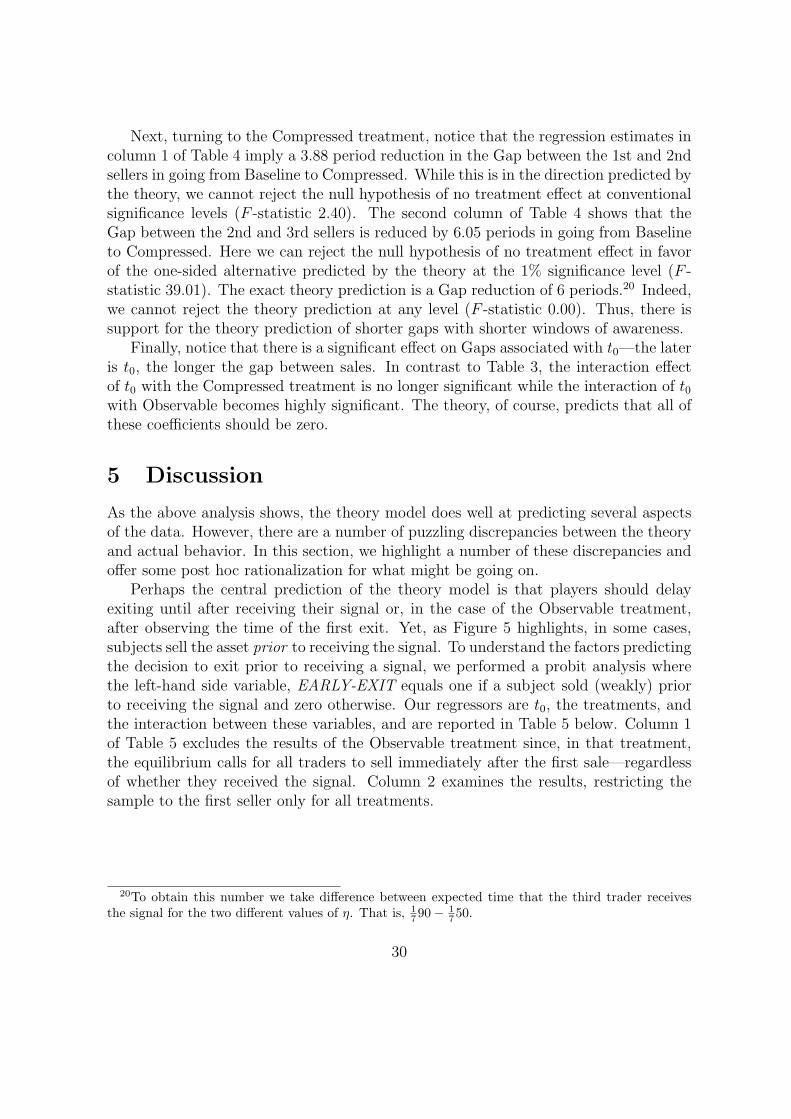
Perhaps the central prediction of the theory model is that players should delayexiting until after receiving their signal or, in the case of the Observable treatment,after observing the time of the first exit. Yet, as Figure 5 highlights, in some cases,subjects sell the asset prior to receiving the signal. To understand the factors predictingthe decision to exit prior to receiving a signal, we performed a probit analysis wherethe left-hand side variable, EARLY-EXIT equals one if a subject sold (weakly) priorto receiving the signal and zero otherwise. Our regressors are t0, the treatments, andthe interaction between these variables, and are reported in Table 5 below. Column 1of Table 5 excludes the results of the Observable treatment since, in that treatment,the equilibrium calls for all traders to sell immediately after the first sale—regardlessof whether they received the signal. Column 2 examines the results, restricting thesample to the first seller only for all treatments.

20To obtain this number we take difference between expected time that the third trader receivesthe signal for the two different values of η. That is, 1

790− 1750.

30

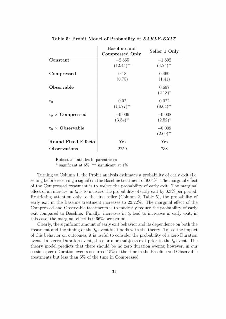
Table 5: Probit Model of Probability of EARLY-EXIT

Baseline andCompressed Only

Seller 1 Only

Constant −2.865 −1.892(12.44)∗∗ (4.24)∗∗

Compressed 0.18 0.469(0.75) (1.41)

Observable 0.697(2.18)∗

t0 0.02 0.022(14.77)∗∗ (8.64)∗∗

t0 × Compressed −0.006 −0.008(3.54)∗∗ (2.52)∗

t0 × Observable −0.009(2.69)∗∗

Round Fixed Effects Yes Yes

Observations 2259 738

Robust z-statistics in parentheses* significant at 5%; ** significant at 1%

Turning to Column 1, the Probit analysis estimates a probability of early exit (i.e.selling before receiving a signal) in the Baseline treatment of 9.04%. The marginal effectof the Compressed treatment is to reduce the probability of early exit. The marginaleffect of an increase in t0 is to increase the probability of early exit by 0.3% per period.Restricting attention only to the first seller (Column 2, Table 5), the probability ofearly exit in the Baseline treatment increases to 22.22%. The marginal effect of theCompressed and Observable treatments is to modestly reduce the probability of earlyexit compared to Baseline. Finally. increases in t0 lead to increases in early exit; inthis case, the marginal effect is 0.66% per period.

Clearly, the significant amount of early exit behavior and its dependence on both thetreatment and the timing of the t0 event is at odds with the theory. To see the impactof this behavior on outcomes, it is useful to consider the probability of a zero Durationevent. In a zero Duration event, three or more subjects exit prior to the t0 event. Thetheory model predicts that there should be no zero duration events; however, in oursessions, zero Duration events occurred 15% of the time in the Baseline and Observabletreatments but less than 5% of the time in Compressed.

31

What accounts for the differences in early exit behavior in the Compressed andObservable treatments compared Baseline? Why does the probability of early exitdepend on the time period of the t0 event? Why are zero duration events more commonin Baseline and Observable compared to the Compressed treatment?

To rationalize the finding that the probability of early exit depends on the timingof the t0 event, suppose that subjects use the following heuristic strategy: A subjecttries to anticipate how far in the past (if at all) the t0 event has occurred. Once theexpected time since the t0 event has occurred grows sufficiently large, a subject willexit. Suppose a subject receives a signal at time t. In that case, the expected time sincethe t0 event has occurred is the same regardless of t owing to the exponential processgenerating t0. Thus, a subject following the heuristic strategy would simply wait afixed number of periods after having received the signal before exiting. Notice thatthe equilibrium strategy derived earlier is a special case of this heuristic. This perhapsexplains the performance of the equilibrium model in predicting the main treatmenteffects we observe despite the apparent complexity of the experimental setting.

Next, suppose that subjects following this heuristic strategy suffer from the follow-ing cognitive bias: Subjects perceive an increasing arrival rate of the t0 event over timeinstead of the actual constant arrival rate. Note that the vast majority of experiencesindividuals have with random arrival processes have increasing, rather than constant,arrival rates. If subjects perceive the arrival rate as increasing, then, as the time periodof the game increases, subjects not receiving a signal think it increasingly likely thatthe t0 event has occurred but they are uninformed about it. Once this becomes suffi-ciently likely, a subject following the heuristic strategy described above will (rationally)choose to exit rather than to stay in the game. Therefore, the incidence of early exitsshould be increasing in t0—across all treatments. This is consistent with the results inTable 5 as well as on the coefficient associated with t0 in explaining Delay in Table 3.

Bias in the perception of arrival rates can also explain differences across treatments.Notice that, in the Compressed treatment, subjects realize that the “window of aware-ness” is shorter and, therefore, correctly perceive that, even if they have not receivedthe signal, the t0 event could not have occurred too far in the past. Hence, the incen-tives to exit early are reduced in this treatment relative to Baseline. In the Observabletreatment, the expectation about the timing of the t0 event is identical to Baseline;however the potential downside from remaining in the game is lower in Observablesince a subject who does not exit early still has a 2 in 5 chance of exiting successfullyafter observing the first exit.

How does this rationale compare with alternative explanations? A simple alterna-tive is that players simply make random errors in their exit times. As we will showbelow, the simplest version of this explanation is unsatisfactory in explaining zero du-ration events in the data. To see this, first consider the Observable treatment. In thistreatment, such errors can give rise to herding behavior and hence to zero durationevents. Formally, suppose that there is a chance ε that each seller sells before t0 and

32

that all others herd immediately after the first sale. Thus, to obtain zero durationevents the observed 13.68% of the time in this model requires that ε solve

1− (1− ε)6 = .1368

which yields an error rate of 2.4%. This does not seem unreasonable given the com-plexity of the experiment. However, applying this same error rate to the Baseline andCompressed treatments does not yield sensible results. Specifically, this same 2.4%error rate leads to the prediction that, in both the Baseline or Compressed treatments,zero duration events occur with probability

6∑j=3

(6j

)εj (1− ε)6−j |ε=.024 = .0003

This is a poor prediction in terms of the levels of zero duration events as well as fordifferences across treatments. (Recall that zero duration events occur approximatelythree times as often in Baseline as in Compressed, yet the error explanation predictsno difference.)

The error explanation is, however, quite useful at explaining the relationship be-tween the timing of the t0 event and the Gap between the first and second sales. Recallfrom Table 4 that in the Baseline and Compressed treatment, the Gap between thefirst and second sales is increasing in t0; whereas in the Observable treatment, it isdecreasing in t0.

Notice however, that the error rationale described above mostly ignores the strate-gic effects of the possibility of errors on equilibrium strategies. If others are makingmistakes, this changes the cost/benefit trade-off for a subject and hence has strate-gic effects and it is possible that these strategic effects might help to rationalize thediscrepancies between the data and the theory model. One avenue to formalize theseideas is to study clock games using the quantal response equilibrium solution concept(see, for example, McKelvey and Palfrey (1995) and Capra, Goeree, Gomez, and Holt(1999)). While this seems promising, the complexity of equilibrium calculation underthe assumption of full rationality led us to leave this analysis for future research.

6 Extending Clock Games: Effects of Information

Clustering

There are two key differences between the “standard” model of clock games we justpresented and its nearest antecedent, the AB model. First, in the standard modelthere are a discrete number of players whereas in AB there is a continuum. Second,in the standard model information is clustered, in the sense that each player possessesa positive fraction of the aggregate information available about t0. In AB, however,

33

information is (uniformly) diffused and each player possesses a zero measure of theaggregate information. In many situations, it seems more realistic to that there areonly a few key players and/or their information is clustered. This is clearly the casein the situation of new product introductions. Similarly, in the situation of a currencyattack, there will only be a few key institutions with the information and the financialresources to move effectively against the central bank. Next, consider the case of thestock market. Here there are many individuals but information is arguably clustered.For instance, suppose that a “cohort” of investors has as their primary news sourceThe Wall Street Journal while others rely mainly on Nightly Business Review. Thedifference in news coverage between these two sources naturally leads to informationclustering.

To isolate the pure effect of information clustering, we extend the basic clock gamesmodel to study a hybrid model consisting of a continuum of individuals but whereinformation clustering is present. We refer to it as the CC (continuum with clustering)model. In this model, players occur on a continuum but are divided into I equal sized“cohorts.” All players in a cohort receive the signal at an identical point in time—soinformation is clustered. The game ends when a mass of players equal to K cohortsdecides to exit. We then study the relation between equilibrium delay in the extendedmodel with the two polar cases—the AB model and the standard Clock Games model—to illustrate the economic effect of information clustering.

Unobservable Actions. We begin by supposing that exit decisions are unobservableand characterizing the set of symmetric equilibria in the CC model. It is useful todefine:

τ (K, I) =1

gln

(λF (K, I, η (λ− g))

g − (g − λ) F (K, I, ηλ)

).

This is identical to the expression for τ given in Proposition 1 but with functionalarguments for K and I added.

Proposition 5 In the CC model, any delay τCC ∈ [τ (K − 1, I) , τ (K, I)] is a sym-metric equilibrium.

Notice that the equilibrium in Proposition 5 exhibiting the longest equilibriumdelay corresponds exactly to the unique symmetric equilibrium in the standard model.Moreover, this equilibrium is the Pareto-best of all the equilibria arising in the CCmodel.

What accounts for the equilibrium multiplicity when there is a continuum of playerscompared to the standard case? The key is that the presence of information clusteringwith a continuum of players introduces a discontinuity in the expected payoffs of playeri in a given cohort. To see this, notice that if player i exits just a bit before his cohort,he faces a trade-off between the gains from waiting versus the chance that the game

34

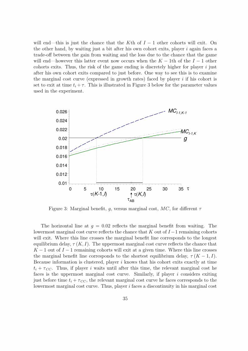
will end—this is just the chance that the Kth of I − 1 other cohorts will exit. Onthe other hand, by waiting just a bit after his own cohort exits, player i again faces atrade-off between the gain from waiting and the loss due to the chance that the gamewill end—however this latter event now occurs when the K − 1th of the I − 1 othercohorts exits. Thus, the risk of the game ending is discretely higher for player i justafter his own cohort exits compared to just before. One way to see this is to examinethe marginal cost curve (expressed in growth rates) faced by player i if his cohort isset to exit at time ti + τ . This is illustrated in Figure 3 below for the parameter valuesused in the experiment.

0.01

0.012

0.014

0.016

0.018

0.02

0.022

0.024

0.026

0 5 10 15 20 25 30 35

g

K-1,I) K,I)

AB

MCI-1,K-1

MCI-1,K

Figure 3: Marginal benefit, g, versus marginal cost, MC, for different τ

The horizontal line at g = 0.02 reflects the marginal benefit from waiting. Thelowermost marginal cost curve reflects the chance that K out of I−1 remaining cohortswill exit. Where this line crosses the marginal benefit line corresponds to the longestequilibrium delay, τ (K, I). The uppermost marginal cost curve reflects the chance thatK − 1 out of I − 1 remaining cohorts will exit at a given time. Where this line crossesthe marginal benefit line corresponds to the shortest equilibrium delay, τ (K − 1, I).Because information is clustered, player i knows that his cohort exits exactly at timeti + τCC . Thus, if player i waits until after this time, the relevant marginal cost hefaces is the uppermost marginal cost curve. Similarly, if player i considers exitingjust before time ti + τCC , the relevant marginal cost curve he faces corresponds to thelowermost marginal cost curve. Thus, player i faces a discontinuity in his marginal cost

35

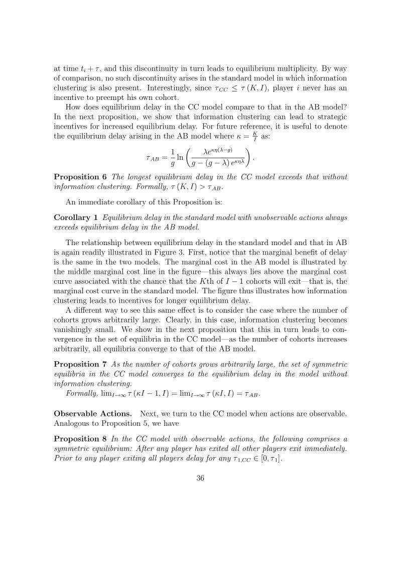
at time ti + τ , and this discontinuity in turn leads to equilibrium multiplicity. By wayof comparison, no such discontinuity arises in the standard model in which informationclustering is also present. Interestingly, since τCC ≤ τ (K, I), player i never has anincentive to preempt his own cohort.

How does equilibrium delay in the CC model compare to that in the AB model?In the next proposition, we show that information clustering can lead to strategicincentives for increased equilibrium delay. For future reference, it is useful to denotethe equilibrium delay arising in the AB model where κ = K

Ias:

τAB =1

gln

(λeκη(λ−g)

g − (g − λ) eκηλ

).

Proposition 6 The longest equilibrium delay in the CC model exceeds that withoutinformation clustering. Formally, τ (K, I) > τAB.

An immediate corollary of this Proposition is:

Corollary 1 Equilibrium delay in the standard model with unobservable actions alwaysexceeds equilibrium delay in the AB model.

The relationship between equilibrium delay in the standard model and that in ABis again readily illustrated in Figure 3. First, notice that the marginal benefit of delayis the same in the two models. The marginal cost in the AB model is illustrated bythe middle marginal cost line in the figure—this always lies above the marginal costcurve associated with the chance that the Kth of I − 1 cohorts will exit—that is, themarginal cost curve in the standard model. The figure thus illustrates how informationclustering leads to incentives for longer equilibrium delay.

A different way to see this same effect is to consider the case where the number ofcohorts grows arbitrarily large. Clearly, in this case, information clustering becomesvanishingly small. We show in the next proposition that this in turn leads to con-vergence in the set of equilibria in the CC model—as the number of cohorts increasesarbitrarily, all equilibria converge to that of the AB model.

Proposition 7 As the number of cohorts grows arbitrarily large, the set of symmetricequilibria in the CC model converges to the equilibrium delay in the model withoutinformation clustering.

Formally, limI→∞ τ (κI − 1, I) = limI→∞ τ (κI, I) = τAB.

Observable Actions. Next, we turn to the CC model when actions are observable.Analogous to Proposition 5, we have

Proposition 8 In the CC model with observable actions, the following comprises asymmetric equilibrium: After any player has exited all other players exit immediately.Prior to any player exiting all players delay for any τ 1,CC ∈ [0, τ 1].

36

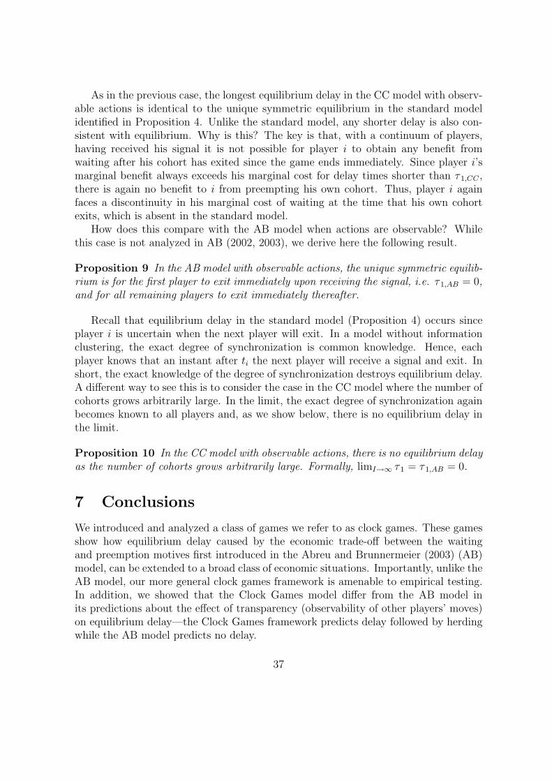
As in the previous case, the longest equilibrium delay in the CC model with observ-able actions is identical to the unique symmetric equilibrium in the standard modelidentified in Proposition 4. Unlike the standard model, any shorter delay is also con-sistent with equilibrium. Why is this? The key is that, with a continuum of players,having received his signal it is not possible for player i to obtain any benefit fromwaiting after his cohort has exited since the game ends immediately. Since player i’smarginal benefit always exceeds his marginal cost for delay times shorter than τ 1,CC ,there is again no benefit to i from preempting his own cohort. Thus, player i againfaces a discontinuity in his marginal cost of waiting at the time that his own cohortexits, which is absent in the standard model.

How does this compare with the AB model when actions are observable? Whilethis case is not analyzed in AB (2002, 2003), we derive here the following result.

Proposition 9 In the AB model with observable actions, the unique symmetric equilib-rium is for the first player to exit immediately upon receiving the signal, i.e. τ 1,AB = 0,and for all remaining players to exit immediately thereafter.

Recall that equilibrium delay in the standard model (Proposition 4) occurs sinceplayer i is uncertain when the next player will exit. In a model without informationclustering, the exact degree of synchronization is common knowledge. Hence, eachplayer knows that an instant after ti the next player will receive a signal and exit. Inshort, the exact knowledge of the degree of synchronization destroys equilibrium delay.A different way to see this is to consider the case in the CC model where the number ofcohorts grows arbitrarily large. In the limit, the exact degree of synchronization againbecomes known to all players and, as we show below, there is no equilibrium delay inthe limit.

Proposition 10 In the CC model with observable actions, there is no equilibrium delayas the number of cohorts grows arbitrarily large. Formally, limI→∞ τ 1 = τ 1,AB = 0.

7 Conclusions

We introduced and analyzed a class of games we refer to as clock games. These gamesshow how equilibrium delay caused by the economic trade-off between the waitingand preemption motives first introduced in the Abreu and Brunnermeier (2003) (AB)model, can be extended to a broad class of economic situations. Importantly, unlike theAB model, our more general clock games framework is amenable to empirical testing.In addition, we showed that the Clock Games model differ from the AB model inits predictions about the effect of transparency (observability of other players’ moves)on equilibrium delay—the Clock Games framework predicts delay followed by herdingwhile the AB model predicts no delay.

37

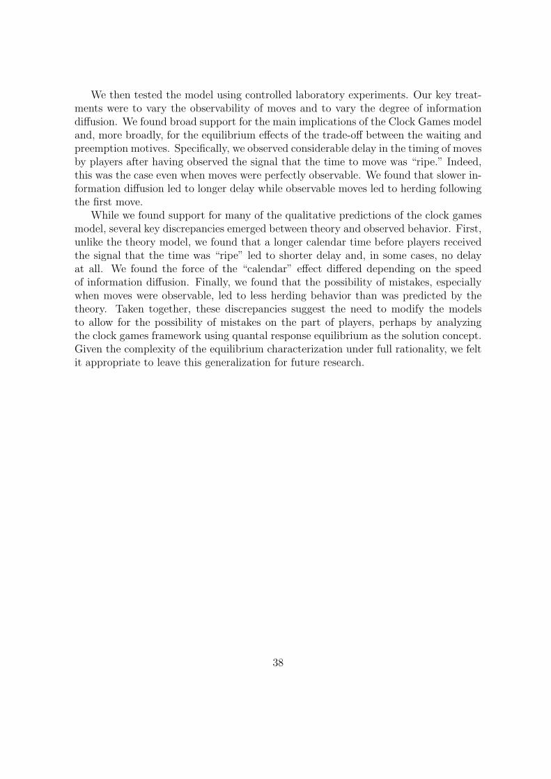
We then tested the model using controlled laboratory experiments. Our key treat-ments were to vary the observability of moves and to vary the degree of informationdiffusion. We found broad support for the main implications of the Clock Games modeland, more broadly, for the equilibrium effects of the trade-off between the waiting andpreemption motives. Specifically, we observed considerable delay in the timing of movesby players after having observed the signal that the time to move was “ripe.” Indeed,this was the case even when moves were perfectly observable. We found that slower in-formation diffusion led to longer delay while observable moves led to herding followingthe first move.

While we found support for many of the qualitative predictions of the clock gamesmodel, several key discrepancies emerged between theory and observed behavior. First,unlike the theory model, we found that a longer calendar time before players receivedthe signal that the time was “ripe” led to shorter delay and, in some cases, no delayat all. We found the force of the “calendar” effect differed depending on the speedof information diffusion. Finally, we found that the possibility of mistakes, especiallywhen moves were observable, led to less herding behavior than was predicted by thetheory. Taken together, these discrepancies suggest the need to modify the modelsto allow for the possibility of mistakes on the part of players, perhaps by analyzingthe clock games framework using quantal response equilibrium as the solution concept.Given the complexity of the equilibrium characterization under full rationality, we feltit appropriate to leave this generalization for future research.

38

References

Abreu, D., and M. K. Brunnermeier (2002): “Synchronization Risk and Delayed Arbi-trage,” Journal of Financial Economics, 66(2-3), 341–360.

(2003): “Bubbles and Crashes,” Econometrica, 71(1), 173–204.

Baye, M. R., D. Kovenock, and C. G. de Vries (1993): “Rigging the Lobbying Process:An Application of the All-Pay Auction,” American Economic Review, 83, 289–294.

Bulow, J., and P. Klemperer (1999): “The Generalized War of Attrition,” AmericanEconomic Review, 89(1), 175–189.

Cabrales, A., R. Nagel, and R. Armenter (2002): “Equilibrium Selection throughIncomplete Information in Coordination Games: An Experimental Study,” UniversitatPompeu Fabra Working Paper, No. 601.

Capra, C. M., J. K. Goeree, R. Gomez, and C. A. Holt (1999): “Anomalous Behaviorin a Traveler’s Dilemma,” American Economic Review, 89(3), 678–690.

Carlsson, H., and E. van Damme (1993): “Global Games and Equilibrium Selection,”Econometrica, 61(5), 989–1018.

Chamley, C., and D. Gale (1994): “Information Revelation and Strategic Delay in aModel of Investment,” Econometrica, 62, 1065–1085.

Fudenberg, D., and J. Tirole (1985): “A Theory of Exit in Duopoly,” Econometrica,54(4), 943–960.

(1991): Game Theory. MIT Press, Cambridge, MA.

Gul, F., and R. Lundholm (1995): “Endogenous Timing and the Clustering of Agents’Decisions,” Journal of Political Economy, 103, 1039–1066.

Harris, C., and J. Vickers (1985): “Perfect Equilibrium in a Model of a Race,” Reviewof Economic Studies, 52(2), 193–209.

Heinemann, F., R. Nagel, and P. Ockenfels (2004): “The Theory of Global Games onTest: Experimental Analysis of Coordination Games with Public and Private Information,”Econometrica, 72(5), 1583–1599.

Hopenhayn, H., and F. Squintani (2006): “Preemption Games with Private Information,”Working paper.

Kummer, E. E. (1836): “Uber die Hypergeometrische Reihe,” Journal fur reine und ange-wandte Mathematik, 15, 39–83.

Leininger, W. (1989): “Escalation and Cooperation in Conflict Situations - The DollarAuction Revisited,” The Journal of Conflict Resolution, 33, 231–254.

39

McKelvey, R. D., and T. R. Palfrey (1992): “An Experimental Study of the CentipedeGame,” Econometrica, 60(4), 803–836.

(1995): “Quantal Response Equilibria for Normal Form Games,” Games and Eco-nomic Behavior, 10(1), 6–38.

Morris, S. (1995): “Co-operation and Timing,” CARESS Working paper 95-05.

Morris, S., and H. Shin (1998): “Unique Equilibrium in a Model of Self-Fulfilling CurrencyAttacks,” American Economic Review, 88(3), 587–596.

Obstfeld, M. (1996): “Models of Currency Crises with Self-Fulfilling Features,” EuropeanEconomic Review, 40, 1037–1047.

O’Neill, B. (1986): “International Escalation and the Dollar Auction,” The Journal ofConflict Resolution, 30, 33–50.

Osborne, M. J. (2003): An Introduction to Game Theory. Oxford University Press, Oxford.

Park, A., and L. Smith (2003): “Caller Number Five: Timing Games that Morph fromOne Form to Another,” Mimeo, University of Michigan.

(2004): “From the Gold Rush to Rush Hour: Timing Models with Both Explosiveand Timed Entry,” Mimeo, University of Michigan.

Reinganum, J. (1981): “Dynamic Games of Innovation,” Journal of Economic Theory, 25,21–41.

Riordan, M. (1992): “Regulation and Preemptive Technology Adoption,” RAND Journalof Economics, 23, 334–349.

Rosenthal, R. (1981): “Games of Perfect Information, Predatory Pricing, and the Chain-Store Paradox,” Journal of Economic Theory, 25, 92–100.

Shubik, M. (1971): “The Dollar Auction Game: A Paradox in Noncooperative Behaviorand Escalation (in Gaming),” Journal of Conflict Resolution, 15(1), 109–111.

Slater, L. J. (1974): “Confluent Hypergeometric Functions,” in Handbook of MathematicalFunctions with Formulas, Graphs, and Mathematical Tables, ed. by M. Abramowitz, andI. A. Stegun, pp. 503–515. Dover, New York, NY, Chapter 13, 9th printing.

Welford, A. T. (1980): Reaction Times. Academic Press, New York.

Zhang, J. (1997): “Strategic Delay and the Onset of Investment Cascades,” Rand Journalof Economics, 28, 188–205.

40

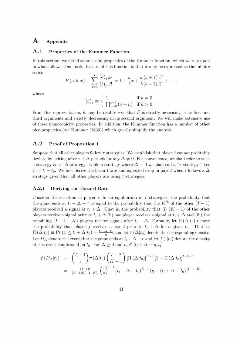
A Appendix

A.1 Properties of the Kummer Function

In this section, we detail some useful properties of the Kummer function, which we rely uponin what follows. One useful feature of this function is that it may be expressed as the infiniteseries

F (a, b, x) ≡∞∑

j=0

(a)j

(b)j

xj

j!= 1 +

a

bx +

a (a + 1)

b (b + 1)

x2

2!+ . . . ,

where

(a)k ≡{

1 if k = 0∏k−1n=0 (a + n) if k > 0

.

From this representation, it may be readily seen that F is strictly increasing in its first andthird arguments and strictly decreasing in its second argument. We will make extensive useof these monotonicity properties. In addition, the Kummer function has a number of othernice properties (see Kummer (1836)) which greatly simplify the analysis.

A.2 Proof of Proposition 1

Suppose that all other players follow τ strategies. We establish that player i cannot profitablydeviate by exiting after τ +∆ periods for any ∆ 6= 0. For convenience, we shall refer to sucha strategy as a “∆ strategy” while a strategy where ∆ = 0 we shall call a “τ strategy.” Letz := ti − t0. We first derive the hazard rate and expected drop in payoff when i follows a ∆strategy given that all other players are using τ strategies.

A.2.1 Deriving the Hazard Rate

Consider the situation of player i. In an equilibrium in τ strategies, the probability thatthe game ends at ti + ∆ + τ is equal to the probability that the Kth of the other (I − 1)players received a signal at ti + ∆. That is, the probability that (i) (K − 1) of the otherplayers receive a signal prior to ti + ∆ (ii) one player receives a signal at ti + ∆ and (iii) theremaining (I − 1−K) players receive signals after ti + ∆. Formally, let Π (∆|t0) denotethe probability that player j receives a signal prior to ti + ∆ for a given t0. That is,Π (∆|t0) ≡ Pr (x ≤ ti + ∆|t0) = ti+∆−t0

η, and let π (∆|t0) denote the corresponding density.

Let D∆ denote the event that the game ends at ti +∆+ τ and let f (·|t0) denote the densityof this event conditional on t0. For ∆ ≥ 0 and t0 ∈ [ti + ∆− η, ti]

f (D∆|t0) =

(I − 1

1

)π (∆|t0)

(I − 2

K − 1

)[Π (∆|t0)]K−1 [1− Π (∆|t0)]I−1−K

= (I−1)!(K−1)!(I−1−K)!

(1η

)I−1

(ti + ∆− t0)K−1 (η − (ti + ∆− t0))

I−1−K .

41

More generally, using z := ti − t0, we have

f (D∆|t0) =

0 for ti + ∆ < t0(I−1)!

(K−1)!(I−1−K)!

(1η

)I−1

(∆ + z)K−1 (η − (∆ + z))I−1−K for ti + ∆ ∈ [t0, t0 + η]

0 for ti + ∆ > t0 + η.

Suppose that at time ti + ∆ + τ , i knows that the game is still ongoing. This meansthat, at most, (K − 1) of the other players received a signal prior to ti + ∆. Let us denotethe event that the game is still “alive” at ti + ∆ + τ by A−

∆.For ∆ ≥ 0 and ti + ∆ ∈ [t0, t0 + η]:

Pr(A−

∆|t0)

=K−1∑n=0

(I − 1

n

)Π (∆|t0)n [1− Π (∆|t0)]I−1−n

=K−1∑n=0

(I − 1)!

n! (I − 1− n)!

(1

η

)I−1

(ti + ∆− t0)n (η − (ti + ∆− t0))

I−1−n .

More generally, using z := ti − t0, we have

Pr(A−

∆|t0)

=

1 for ti + ∆ < t0K−1∑n=0

(I−1)!n!(I−1−n)!

(1η

)I−1

(z + ∆)n (η − (z + ∆))I−1−n for ti + ∆ ∈ [t0, t0 + η]

0 for ti + ∆ > t0 + η

However, player i does not know t0. Hence, we have to take expectations over all possiblet0. Recall that t0 is exponentially distributed, with p.d.f.

φ (t0) = λe−λt0 .

Further, i’s signal, ti, implies that ti − η ≤ t0 ≤ ti, hence

φ (t0|ti) =λe−λt0

1− e−λti − (1− e−λ(ti−η))

=λeλz

eλη − 1.

Thus, player i’s hazard rate of the game ending at time ti + ∆ + τ is

h (∆, ti) =f (D∆|ti)Pr

(A−

∆|ti)

=

ti∫ti−η

φ (t0|ti) f (D∆|t0) dt0

ti∫ti−η

φ (t0|ti) Pr(A−

∆|t0)dt0

.

42

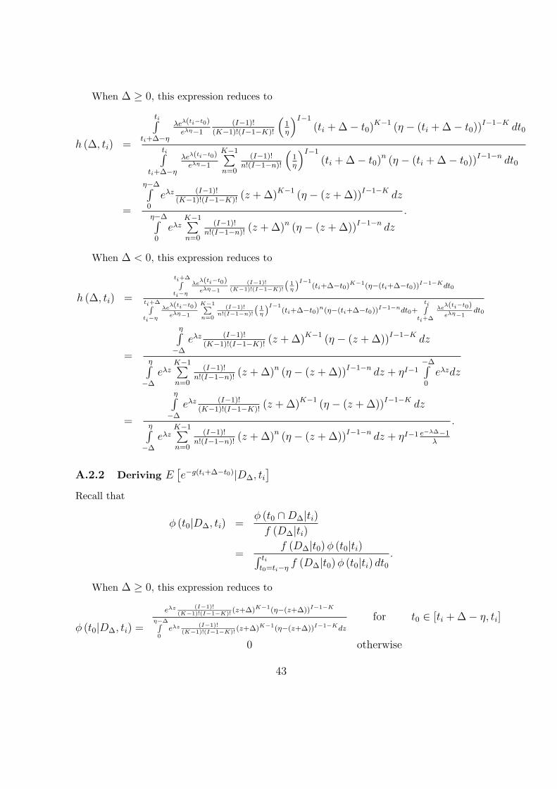
When ∆ ≥ 0, this expression reduces to

h (∆, ti) =

ti∫ti+∆−η

λeλ(ti−t0)

eλη−1(I−1)!

(K−1)!(I−1−K)!

(1η

)I−1

(ti + ∆− t0)K−1 (η − (ti + ∆− t0))

I−1−K dt0

ti∫ti+∆−η

λeλ(ti−t0)

eλη−1

K−1∑n=0

(I−1)!n!(I−1−n)!

(1η

)I−1

(ti + ∆− t0)n (η − (ti + ∆− t0))

I−1−n dt0

=

η−∆∫0

eλz (I−1)!(K−1)!(I−1−K)!

(z + ∆)K−1 (η − (z + ∆))I−1−K dz

η−∆∫0

eλzK−1∑n=0

(I−1)!n!(I−1−n)!

(z + ∆)n (η − (z + ∆))I−1−n dz

.

When ∆ < 0, this expression reduces to

h (∆, ti) =

ti+∆Rti−η

λeλ(ti−t0)

eλη−1

(I−1)!(K−1)!(I−1−K)!(

1η )

I−1(ti+∆−t0)K−1(η−(ti+∆−t0))I−1−Kdt0

ti+∆Rti−η

λeλ(ti−t0)

eλη−1

K−1Pn=0

(I−1)!n!(I−1−n)!(

1η )

I−1(ti+∆−t0)n(η−(ti+∆−t0))I−1−ndt0+

tiRti+∆

λeλ(ti−t0)

eλη−1dt0

=

η∫−∆

eλz (I−1)!(K−1)!(I−1−K)!

(z + ∆)K−1 (η − (z + ∆))I−1−K dz

η∫−∆

eλzK−1∑n=0

(I−1)!n!(I−1−n)!

(z + ∆)n (η − (z + ∆))I−1−n dz + ηI−1−∆∫0

eλzdz

=

η∫−∆

eλz (I−1)!(K−1)!(I−1−K)!

(z + ∆)K−1 (η − (z + ∆))I−1−K dz

η∫−∆

eλzK−1∑n=0

(I−1)!n!(I−1−n)!

(z + ∆)n (η − (z + ∆))I−1−n dz + ηI−1 e−λ∆−1λ

.

A.2.2 Deriving E[e−g(ti+∆−t0)|D∆, ti

]

Recall that

φ (t0|D∆, ti) =φ (t0 ∩D∆|ti)

f (D∆|ti)=

f (D∆|t0) φ (t0|ti)∫ tit0=ti−η

f (D∆|t0) φ (t0|ti) dt0.

When ∆ ≥ 0, this expression reduces to

φ (t0|D∆, ti) =

eλz (I−1)!(K−1)!(I−1−K)!

(z+∆)K−1(η−(z+∆))I−1−K

η−∆R0

eλz (I−1)!(K−1)!(I−1−K)!

(z+∆)K−1(η−(z+∆))I−1−Kdz

for t0 ∈ [ti + ∆− η, ti]

0 otherwise

43

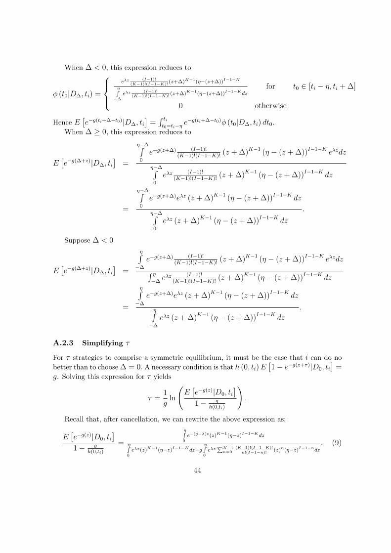
When ∆ < 0, this expression reduces to

φ (t0|D∆, ti) =

eλz (I−1)!(K−1)!(I−1−K)!

(z+∆)K−1(η−(z+∆))I−1−K

ηR−∆

eλz (I−1)!(K−1)!(I−1−K)!

(z+∆)K−1(η−(z+∆))I−1−Kdzfor t0 ∈ [ti − η, ti + ∆]

0 otherwise

Hence E[e−g(ti+∆−t0)|D∆, ti

]=

∫ tit0=ti−η

e−g(ti+∆−t0)φ (t0|D∆, ti) dt0.When ∆ ≥ 0, this expression reduces to

E[e−g(∆+z)|D∆, ti

]=

η−∆∫0

e−g(z+∆) (I−1)!(K−1)!(I−1−K)!

(z + ∆)K−1 (η − (z + ∆))I−1−K eλzdz

η−∆∫0

eλz (I−1)!(K−1)!(I−1−K)!

(z + ∆)K−1 (η − (z + ∆))I−1−K dz

=

η−∆∫0

e−g(z+∆)eλz (z + ∆)K−1 (η − (z + ∆))I−1−K dz

η−∆∫0

eλz (z + ∆)K−1 (η − (z + ∆))I−1−K dz

.

Suppose ∆ < 0

E[e−g(∆+z)|D∆, ti

]=

η∫−∆

e−g(z+∆) (I−1)!(K−1)!(I−1−K)!

(z + ∆)K−1 (η − (z + ∆))I−1−K eλzdz

∫ η

−∆eλz (I−1)!

(K−1)!(I−1−K)!(z + ∆)K−1 (η − (z + ∆))I−1−K dz

=

η∫−∆

e−g(z+∆)eλz (z + ∆)K−1 (η − (z + ∆))I−1−K dz

η∫−∆

eλz (z + ∆)K−1 (η − (z + ∆))I−1−K dz

.

A.2.3 Simplifying τ

For τ strategies to comprise a symmetric equilibrium, it must be the case that i can do nobetter than to choose ∆ = 0. A necessary condition is that h (0, ti) E

[1− e−g(z+τ)|D0, ti

]=

g. Solving this expression for τ yields

τ =1

gln

(E

[e−g(z)|D0, ti

]

1− gh(0,ti)

).

Recall that, after cancellation, we can rewrite the above expression as:

E[e−g(z)|D0, ti

]

1− gh(0,ti)

=

ηR0

e−(g−λ)z(z)K−1(η−z)I−1−Kdz

ηR0

eλz(z)K−1(η−z)I−1−Kdz−gηR0

eλzPK−1

n=0(K−1)!(I−1−K)!

n!(I−1−n)!(z)n(η−z)I−1−ndz

. (9)

44

Now, let Num and Den denote, respectively, the numerator and denominator of the right-hand side of equation (9) . By series expansion of the exponential function it follows that

Num =ηI−1Γ (I −K) Γ (K)

Γ (I)F (K, I, η (λ− g))

Den =ηI−1Γ (I −K) Γ (K)

Γ (I)

[F (K, I, ηλ)− ηg

I

K−1∑n=0

F (1 + n, 1 + I, ηλ)

],

where Γ (·) is the Gamma function satisfying Γ (a) = (a− 1)! for a positive integer a andF (·) is the Kummer function defined above.

In the expression for Den,

K−1∑n=0

F (1 + n, 1 + I, ηλ) =K−1∑n=0

∞∑j=0

(1 + n)j

(1 + I)j

(ηλ)j

j!

=∞∑

j=0

1

(1 + I)j

(ηλ)j

j!

K−1∑n=0

(1 + n)j

=∞∑

j=0

1

(1 + I)j

(ηλ)j

j!

(K)j+1

j + 1.

The last equality follows from∑K−1

n=0 (1 + n)j =(K)j+1

j+1. Therefore,

ηg

I

K−1∑n=0

F (1 + n, 1 + I, ηλ) =g

λ

∞∑j=0

(K)j+1

(I)j+1

(ηλ)j+1

(j + 1)!

=g

λ

∞∑j=1

(K)j

(I)j

(ηλ)j

j!

=g

λ[F (K, I, ηλ)− 1] .

Hence,

Den =ηI−1Γ (I −K) Γ (K)

Γ (I)

[(1− g

λ

)F (K, I, ηλ) +

g

λ

].

Therefore,

τ =1

gln

λF (K, I, η (λ− g))

g − (g − λ) F (K, I, ηλ).

Next, we show that for η ∈ [0, η] , τ > 0. Since E[e−g(z)|D0, ti

]> 0, the following

lemma is sufficient.

45

Lemma 1 h (0, ti) > g.

Proof. Since η < η, λ < g, and F is increasing in its third argument, it then follows that

E[e−g(z)|D0, ti

]

1− gh(0,ti)

=λF (K, I, η (λ− g))

g − (g − λ) F (K, I, ηλ)

>λF (K, I, η (λ− g))

g − (g − λ) F (K, I, ηλ)

=λF (K, I, η (λ− g))

g − (g − λ)(

IgIg−(I−K+1)λ

)

> F (K, I, η (λ− g)) > 0. ¥

A.2.4 Global Deviation

We are now in a position to show that ∆ strategies do not constitute profitable globaldeviations. A necessary condition for an equilibrium is that the “marginal cost” for the∆ = 0 strategy is equal to the (constant) “marginal benefit” of g. To show that there is noprofitable global deviation, it is sufficient to show that the marginal costs are increasing in∆.

The marginal cost of a ∆ strategy (conditional on ti) is

MC (∆|ti) = h (∆, ti)(1− e−gτE

[e−g(ti+∆−t0)|D∆, ti

])

= h (∆, ti)

(1− h (0, ti)− g

h (0, ti) E [e−g(ti−t0)|Dti , ti]E

[e−g(ti+∆−t0)|D∆, ti

])

=h (∆, ti)

h (0, ti)

(h (0, ti) + (g − h (0, ti))

(E

[e−g(ti+∆−t0)|D∆, ti

]

E [e−g(ti−t0)|Dti , ti]

)).

It sufficient to show that h (∆, ti) is increasing in ∆ and E[e−g(ti+∆+τ−t0)|D∆, ti

]is de-

creasing in ∆.Claim 1: Suppose that ∆ ∈ [0, η], then h (∆, ti) is increasing in ∆.Proof: First, define a := z + ∆. Then we can rewrite

h (∆, ti) =

(I−1)!(K−1)!(I−1−K)!

η∫∆

eλa (a)K−1 (η − a)I−1−K da

K−1∑n=0

(I−1n

) η∫∆

eλa (a)n (η − (a))I−1−n da

.

Next, differentiate h (∆, ti) with respect to ∆. The sign of this derivative takes on the signof

46

−eλ∆ (∆)K−1 (η −∆)I−1−KK−1∑n=0

(I−1n

) η∫

∆

eλa (a)n (η − (a))I−1−n da

+K−1∑n=0

(I−1n

)eλ∆ (∆)n (η −∆)I−1−n

η∫

∆

eλa (a)K−1 (η − a)I−1−K da.

We can then rewrite this expression as

−K−1∑n=0

(I−1n

)(∆)K−1 (η −∆)I−1−K

η∫

∆

eλa (a)n (η − a)I−1−n da

+K−1∑n=0

(I−1n

)(∆)n (η −∆)I−1−n

η∫

∆

eλa (a)K−1 (η − a)I−1−K da

= −K−1∑n=0

(I−1n

)(∆)n (η −∆)I−1−K

η∫

∆

eλa (∆)K−1−n (a)n (η − a)I−1−n da

+K−1∑n=0

(I−1n

)(∆)n (η −∆)I−1−K

η∫

∆

eλa (a)K−1 (η −∆)K−n (η − a)I−1−K da > 0,

where the inequality follows from the fact that a > ∆ and η−∆ > η− a for almost all a.¤Claim 2: Suppose that ∆ ∈ [0, η], then E

[e−g(z+∆−t0)|D∆, ti

]is decreasing in ∆.

Proof. Recall that

E[e−g(z+∆−t0)|D∆, ti

]=

∫ η

∆e−gaeλa (a)K−1 (η − a)I−1−K da∫ η

∆eλa (a)K−1 (η − a)I−1−K da

Next, differentiate E[e−g(z+∆−t0)|D∆, ti

]with respect to ∆. The sign of this derivative takes

on the sign of

−e−g∆eλ∆ (∆)K−1 (η −∆)I−1−K

∫ η

∆

eλa (a)K−1 (η − a)I−1−K da

+eλ∆ (∆)K−1 (η −∆)I−1−K

∫ η

∆

e−gaeλa (a)K−1 (η − a)I−1−K da

∝∫ η

∆

−e−g∆eλa (a)K−1 (η − a)I−1−K da +

∫ η

∆

e−gaeλa (a)K−1 (η − a)I−1−K da

=

∫ η

∆

(e−ga − e−g∆

)eλa (a)K−1 (η − a)I−1−K da < 0,

47

where the inequality follows from the fact that a > ∆.¤Claim 3: Suppose that ∆ ∈ [−max {η, τ} , 0] . Then h (∆, ti) is increasing in ∆.Proof. First, define b := η − (z + ∆) , then we can rewrite:

h (∆, ti) =

(I−1)!(K−1)!(I−1−K)!

η∫−∆

eλ(η−∆−b) (η − b)K−1 (b)I−1−K db

η∫−∆

eλ(η−∆−b)K−1∑n=0

(I−1n

)(η − b)n (b)I−1−n db + ηI−1 e−λ∆−1

λ

=

(I−1)!(K−1)!(I−1−K)!

η∫−∆

e−λb (η − b)K−1 (b)I−1−K db

η∫−∆

e−λbK−1∑n=0

(I−1n

)(η − b)n (b)I−1−n db + e−λ(η−∆)ηI−1 e−λ∆−1

λ

=

(I−1)!(K−1)!(I−1−K)!

η∫−∆

e−λb (η − b)K−1 (b)I−1−K db

K−1∑n=0

(I−1n

) η∫−∆

e−λb (η − b)n (b)I−1−n db + ηI−1e−λη 1−eλ∆

λ

.

Next, differentiate h (∆, ti) with respect to ∆. The sign of this derivative takes on thesign of

eλ∆ (η + ∆)K−1 (−∆)I−1−K

K−1∑n=0

(I−1n

) η∫

−∆

e−λb (η − b)n (b)I−1−n db + ηI−1e−λη 1− eλ∆

λ

−[

K−1∑n=0

(I−1n

)eλ∆ (η + ∆)n (−∆)I−1−n − ηI−1e−ληeλ∆

] η∫

−∆

e−λb (η − b)K−1 (b)I−1−K db

First, note that two the non-sum terms are positive.

eλ∆ (η + ∆)K−1 (−∆)I−1−K ηI−1e−λη 1− eλ∆

λ+ ηI−1e−ληeλ∆

η∫

−∆

e−λb (η − b)K−1 (b)I−1−K db

= eλ∆e−ληηI−1

(η + ∆)K−1 (−∆)I−1−K 1− eλ∆

λ+

η∫

−∆

e−λb (η − b)K−1 (b)I−1−K db

> 0,

since 1− eλ∆ > 0.

48

Next, we show that the sum terms are positive.

eλ∆ (η + ∆)K−1 (−∆)I−1−KK−1∑n=0

(I−1n

) ∫ η

−∆

e−λb (η − b)n (b)I−1−n db

−K−1∑n=0

(I−1n

)eλ∆ (η + ∆)n (−∆)I−1−n

∫ η

−∆

e−λb (η − b)K−1 (b)I−1−K db

=K−1∑n=0

(I−1n

)eλ∆ (η + ∆)K−1 (−∆)I−1−K

∫ η

−∆

e−λb (η − b)n (b)I−1−n db

−K−1∑n=0

(I−1n

)eλ∆ (η + ∆)n (−∆)I−1−n

∫ η

−∆

e−λb (η − b)K−1 (b)I−1−K db

=K−1∑n=0

(I−1n

)eλ∆ (η + ∆)n (−∆)I−1−K

η∫

−∆

e−λb (η + ∆)K−1−n (η − b)n (b)I−1−n db

−K−1∑n=0

(I−1n

)eλ∆ (η + ∆)n (−∆)I−1−K

η∫

−∆

e−λb (η − b)K−1 (−∆)K−n (b)I−1−K db > 0,

where the inequality follows from the fact that b > −∆.¤Claim 4: Suppose that ∆ ∈ [−max {η, τ} , 0] , then E

[e−g(z+∆−t0)|D∆, ti

]is decreasing

in ∆.Proof. Recall that

E[e−g(z+∆−t0)|D∆, ti

]=

∫ η+∆

0e−g(a)eλ(a−∆) (a)K−1 (η − a)I−1−K da∫ η+∆

0eλ(a−∆) (a)K−1 (η − a)I−1−K da

=

∫ η+∆

0e−g(a)eλa (a)K−1 (η − a)I−1−K da∫ η+∆

0eλa (a)K−1 (η − a)I−1−K da

Next, differentiate E[e−g(z+∆−t0)|D∆, ti

]with respect to ∆. The sign of this derivative

takes on the sign of

e−g(η+∆)eλ(η+∆) (η + ∆)K−1 (−∆)I−1−K

∫ η+∆

0

eλa (a)K−1 (η − a)I−1−K da

−eλ(η+∆) (η + ∆)K−1 (−∆)I−1−K

∫ η+∆

0

e−g(a)eλa (a)K−1 (η − a)I−1−K da

∝η+∆∫

0

e−g(η+∆)eλa (a)K−1 (η − a)I−1−K da−η+∆∫

0

e−g(a)eλa (a)K−1 (η − a)I−1−K da < 0,

49

where the inequality follows from the fact that a < η + ∆.¤Suppose that ∆ > η. In that case, i exits after ti + η + τ , at which point the game has

already ended with certainty. This strategy is dominated by exiting at ti. Finally, suppose ichooses to exit before becoming informed. Notice that h (−τ , ti) > h where h is the hazardrate associated with exiting before getting a signal; hence, exiting at ti dominates exitingbefore receiving a signal.

A.2.5 Uniqueness of Symmetric Equilibria

So far, we have shown the τ strategies comprise a symmetric equilibrium in clock games. Next,we establish that these strategies constitute the unique symmetric equilibrium. Suppose not,then there exists some other delay time τ ′ 6= τ such that the marginal benefit=marginal costcondition is satisfied. That is, given that all players wait τ ′ periods,

hti+τ ′E[1− e−g(ti+τ ′−t0)|·

]= g.

where hti+τ ′ represents the hazard rate when all players including i play τ ′ strategies. Noticethat since equilibrium play involves merely symmetrically shifting the delay time from τ toτ ′ periods, the hazard rate is unchanged. That is,

hti+τ ′ = h (0, ti) .

The term E[1− e−g(ti+τ ′−t0)|·]; however, is increasing in τ ′; therefore, for all τ ′ 6= τ , it

immediately follows that

hti+τ ′E[1− e−g(ti+τ ′−t0)|·

]= h (0, ti) E

[1− e−g(ti+τ ′−t0)|·

]6= g.

This completes the proof of Proposition 1.¥

A.3 Proof of Proposition 2

Recall that τ = 1gln λF (K,I,η(λ−g))

g−(g−λ)F (K,I,ηλ). We first show that when η = 0, τ = 0. From the series

expansion of F (·) it can easily be seen that F (K, I, 0) = 1, hence when η = 0, τ = 0.For η ∈ (0, η),

λF (K, I, η (λ− g))

g − (g − λ) F (K, I, ηλ)=

1 +η∫0

∂∂w

F (K, I, w (λ− g))∣∣w=z

dz

1− g−λλ

η∫0

∂∂w

F (K, I, wλ)∣∣w=z

dz

.

50

Using the fact that ∂∂x

F (a, b, x) = abF (a + 1, b + 1, x) , it follows that the right-hand side

may be rewritten as

=

1− (g−λ)KI

∫ η

0

F (K + 1, I + 1, z (λ− g)) dz

1− (g−λ)KI

∫ η

0

F (K + 1, I + 1, zλ) dz

= 1 +

(g−λ)KI

∫ η

0

F (K + 1, I + 1, zλ)− F (K + 1, I + 1, z (λ− g)) dz

1− (g−λ)KI

∫ η

0

F (K + 1, I + 1, zλ) dz

.

That this expression is increasing in η follows from the fact that F (·) is increasing in itsthird argument.¥

A.4 Proof of Proposition 4

It is straightforward to obtain expressions for h1 (0, ti) and E[e−g(z)|D0, ti

]. Simply use the

analogous expressions given in the proof of Proposition 1 and substitute K = 1. This yields

τ 1 =1

gln

( R η0 e−(g−λ)z(η−z)I−2dzR η

0 eλz(η−z)I−2dz− IgI−K+1

R η0 eλz (I−2)!

(I−1)!(η−z)I−1dz

).

Using steps analogous to the simplification of τ , we have

τ 1 =1

gln

(λF (1,I,η(−g+λ))

IgI−K+1

−( IgI−K+1

−λ)F (1,I,ηλ)

).

Since the monotonicity conditions in the proof of Proposition 1 continue to hold in thepresent setting, global deviations from τ 1 strategies are not profitable. It remains only toshow that τ 1 > 0. Since E

[e−g(z)|D0, ti

]> 0, the required inequality follows from

Lemma 2 h1 > IgI−K+1

.

Proof. Following the identical steps in the proof of Lemma 1, we obtain

E[e−g(z)|D0, ti

]

1− g1

h1

= λF (1,I,η(−g+λ))

(λ− IgI−K+1)F (1,I,ηλ)+ Ig

I−K+1

≥ 0, (10)

which is satisfied since η ≤ η.¥Thus, we have shown that τ 1 strategies comprise a symmetric equilibrium. The fact that

τ 1 is the unique symmetric equilibrium follows using steps identical to those in Proposition1.¥

51

A.5 Proof of Proposition 3

Proof. Following observing the first exit, the identity of the last “type” to exit in the con-tinuation game is commonly known. Formally, fix a perfect Bayesian equilibrium in thecontinuation game following the first exit. Let h (ti) be the (endogenous) hazard rate of thegame ending associated with type ti. Define the set of “last” types as:

L = {ti : h (ti) > k} ,

where k is some sufficiently large but finite constant amount. Notice that there is at least onecommonly known type facing an infinite hazard rate. Moreover, there is a positive measureof types facing arbitrarily large hazard rates. These types are in the set L. Notice that, sincethe (growth) benefit of waiting an additional period is at most g, these types have a profitabledeviation of exiting before the time indicated in the equilibrium. But this is a contradiction.Therefore, the unique continuation PBE is where all types exit immediately after observingthe first exit.

A.6 Proofs of Subsection 6

Lemma 3 τ (K − 1, I) < τ (K, I).

Proof. The inequality follows from the fact that F (a, b, x) is increasing in its firstargument.¥

Proof of Proposition 5From Lemma 3, the interval [τ (K − 1, I) , τ (K, I)] is non-empty. To see that τCC ∈

[τ (K − 1, I) , τ (K, I)] comprise a symmetric equilibrium, fix the strategies of all playersother than i at τCC ∈ [τ (K − 1, I) , τ (K, I)] and consider a deviation by player i to sometime ti + τCC + ∆. Using reasoning identical to that used in the proof of Proposition 1, onecan show that if local deviations are not profitable then global deviations are likewise notprofitable. Thus, it suffices to show that local deviations are not profitable. This requires

lim∆↗0

h (∆, ti)(1− e−gτCCE

[e−g(ti+∆−t0)|D∆, ti

]) ≤ g

andlim∆↘0

h (∆, ti)(1− e−gτCCE

[e−g(ti+∆−t0)|D∆, ti

]) ≥ g.

The reason for taking left and right hand limits separately is that a positive mass of playersof size 1/I are known by player i to be exiting at ti + τCC .

First consider a deviation from below.

52

lim∆↗0

h (∆, ti)(1− e−gτCCE

[e−g(ti+∆−t0)|D∆, ti

])

= λF (K, I, ηλ)− e−gτCCF (K, I, (λ− g) η)

[F (K, I, ηλ)− 1]

≤ λF (K, I, ηλ)− e−gτ(K,I)F (K, I, (λ− g) η)

[F (K, I, ηλ)− 1]= g,

where the inequality follows from the definition of τ (K − 1, I) and the fact thatlim∆↗0 h (∆, ti)

(1− e−gτCCE

[e−g(ti+∆−t0)|D∆, ti

])is increasing in τCC .

Next, notice that

lim∆↘0

h (∆, ti)(1− e−gτCCE

[e−g(ti+∆−t0)|D∆, ti

])

= λF (K − 1, I, ηλ)− e−gτCCF (K − 1, I, (λ− g) η)

[F (K − 1, I, ηλ)− 1]

≥ λF (K − 1, I, ηλ)− e−gτ(K−1,I)F (K − 1, I, (λ− g) η)

[F (K − 1, I, ηλ)− 1]= g,

where the inequality follows from the definition of τ (K, I) and the fact thatlim∆↘0 h (∆, ti)

(1− e−gτCCE

[e−g(ti+∆−t0)|D∆, ti

])is increasing in τCC .Therefore, τCC

strategies comprise a symmetric equilibrium.¥

Proof of Proposition 6Define κ ≡ K

I. It is sufficient to show

λF (κI, I,−η (g − λ))

g − (g − λ) F (κI, I, ηλ)>

λe−κη(g−λ)

g − (g − λ) eκηλ.

To obtain the required inequality, it suffices to show F (κI, I, x) > eκx for x 6= 0 andκ ∈ (0, 1). When x > 0, F (κI, I, x)

= 1 +κI

Ix +

κI (κI + 1)

I (I + 1)

x2

2!+

κI (κI + 1) (κI + 2)

I (I + 1) (I + 2)

x3

3!+ ...

= 1 +κI

Ix +

κI (κ (I + 1) + (1− κ))

I (I + 1)

x2

2!+

κI (κ (I + 1) + (1− κ)) (κ (I + 2) + 2 (1− κ))

I (I + 1) (I + 2)

x3

3!+ ...

> 1 +κI

Ix +

κI (κ (I + 1))

I (I + 1)

x2

2!+

κIκ (I + 1) (κ (I + 2))

I (I + 1) (I + 2)

x3

3!+ ... = eκx.

For x < 0,F (κI, I, x) = exF ((1− κ) I, I,−x) .

Using the same steps as above, note F ((1− κ) I, I,−x) > e−(1−κ)x. Hence, F (κI, I, x) >eκx.¥

53

Proof of Proposition 7Recall that,

limI→∞

F (κI, I, x) = 1 + κx + κ2x2

2!+ κ3x3

3!+ . . . = eκx.

Hence,

limI→∞

τ (κI, I) = limI→∞

(1

gln

F (κI, I, η (λ− g))gλ− g−λ

λF (κI, I, ηλ)

),

=1

gln

(λeκη(λ−g)

g − (g − λ) eκηλ

)= τAB.

Similarly, limI→∞ F (κI − 1, I, x) = eκx and hence,

limI→∞

τ (κI − 1, I) = τAB ¥

Proof of Proposition 8Recall that τ 1 is an equilibrium when there is a discrete number, I, of players. From the

series expansion of F , we have that F (0, I, x) = 1. Then, using steps identical to those inProposition 5 yields the result.¥

Proof of Proposition 9First notice that Proposition 3 directly applies; therefore, all remaining players immediately

exit following the first player’s exit. Next, fix an equilibrium where τ 1,CC ≥ 0. Notice that,in such an equilibrium, the hazard rate, h1, at time ti + τ 1,CC must be infinite. This isbecause another player is certain to exit at the next instant. Further, at time ti + τ 1,CC ,player i also infers that he is the first person to receive the signal (otherwise the game wouldalready have ended) hence ti = t0. Together, these two observations imply that

τ 1,AB =1

g

[ln

h1

h1 − g I−1I−K

+ ln E[e−g(ti−t0)|D0, ti

]]

= 0 ¥

Proof of Proposition 10. Define κ ≡ KI

and recall that limb→∞ F (1, b, x) = 1

limI→∞

τ 1 = limI→∞

1

gln

(λF (1,I,η(−g+λ))

IgI(1−κ)+1

−( IgI(1−κ)+1

−λ)F (1,I,ηλ)

)

=1

gln (1) = 0 ¥

54

Appendix B: Instructions Note: Terms in {.} are included only in the COMPRESSED treatments while terms in [.] are included only in OBSERVABLE treatments. Thank you for participating in this experiment on the economics of investment decision making. If you follow the instructions carefully and make good decisions you can earn a considerable amount of money. At the end of the experiment you will be paid in cash and in private. The experiment will take about an hour and a half. There are 12 people participating in this session. They have all been recruited in the same way that you have and are reading the same instructions that you are for the first time. Please refrain from talking to the other participants during the experiment. You are about the play the same selling game 45 times in succession. Each round represents one trading period and each person in the room is a seller in the game. There are two games running simultaneously, so you will not know which game you are in and which players in the room you are playing with. The sellers are randomly matched at the beginning of each period and thus the composition of sellers for each game changes from trading period to trading period. How to play the game: Initially, everyone needs to login from the login page. The game begins after five other players log in (see Figure B1). At the start of each trading period, the price of everyone’s asset begins at 1 ECU (experimental currency units) and increases exponentially. The true value of the asset is predetermined when the game starts. At one point, you will be notified that the current price of the asset exceeds its true value. At that time, the price of the asset will change from red to green. In addition, you will be given the minimum and maximum values of the asset. The true value of the asset lies between those two values (see Figure B2). [In addition, whenever any other seller in your game chooses to sell, you will be notified of this fact by a message at the bottom of your screen indicating the price at which the sale occurred.] Please note that the speed to which the price rises will vary slightly. This is due to random network traffic. How to Sell: In each period, you make your decision of selling your asset by moving the mouse pointer into blue “Sell” box on your screen. DO NOT CLICK THE MOUSE BUTTON. Once you have decided to sell, you have no more decisions to make in the trading period. Your decision is final. There are two ways a trading period can end: (1) Once the third seller moves his/her mouse into the blue window, the period ends; (2) If fewer than three sellers sell, then the trading period ends once a pre-determined number of seconds has elapsed after the asset reaches its true value.

If you sell, you earn an amount in ECUs equals to the price you sell at. If you don’t sell, you will earn the true value of the asset. Please keep in mind that your goal is to maximize your earnings. At the end of each trading period, the true value of the asset, your earnings for this period, your cumulative earnings, and the earnings of other players will all be displayed on your screen (see Figure B3). Click the “Play Again” link on the screen to play the next round. The new round will begin when every player has clicked the link. At the conclusion of the experiment, your total earnings in ECUs will be converted to cash at the rate of 50 ECU = $1. At some point during the trading period, you will receive a message indicating that the current price of the asset has exceeded its “true value”. When you receive this message, the computer will also inform you of the minimum and maximum “true values” for the asset. Are there any questions? Details – This section contains technical details about the game At the start of each selling game, the price of the asset begins at 1 ECU (experimental currency units). The price of the asset increases by 2% in each trading period (which lasts about half a second). You will see the price increasing on your computer screen---the current price is the same for all sellers. In addition, the computer secretly determines the true value of the asset. The shadow value increases with the price of the asset until the computer determines that it has stopped growing. In each trading period, there is a 1% chance that the true value will stop growing. The true value of the asset is the same for you and the other five sellers with whom you are participating. Delayed Information Once the computer determines that the true value has stopped growing, you will be alerted of this fact, but with a random delay. The computer will choose a random delay from zero, one, two, up to ninety {fifty} trading periods (equally likely) for each seller. So on average, the delay will be about 45 {25} seconds from the time the shadow value stopped growing until the time you become informed of this fact. After this delay, you will see a message on your computer screen indicating that the true value has stopped growing as well as displaying the highest and lowest amounts the shadow value could be. The same is true for the other five players, but the computer determines their delay separately your delay. That is, most likely they hear the news at different points in time.

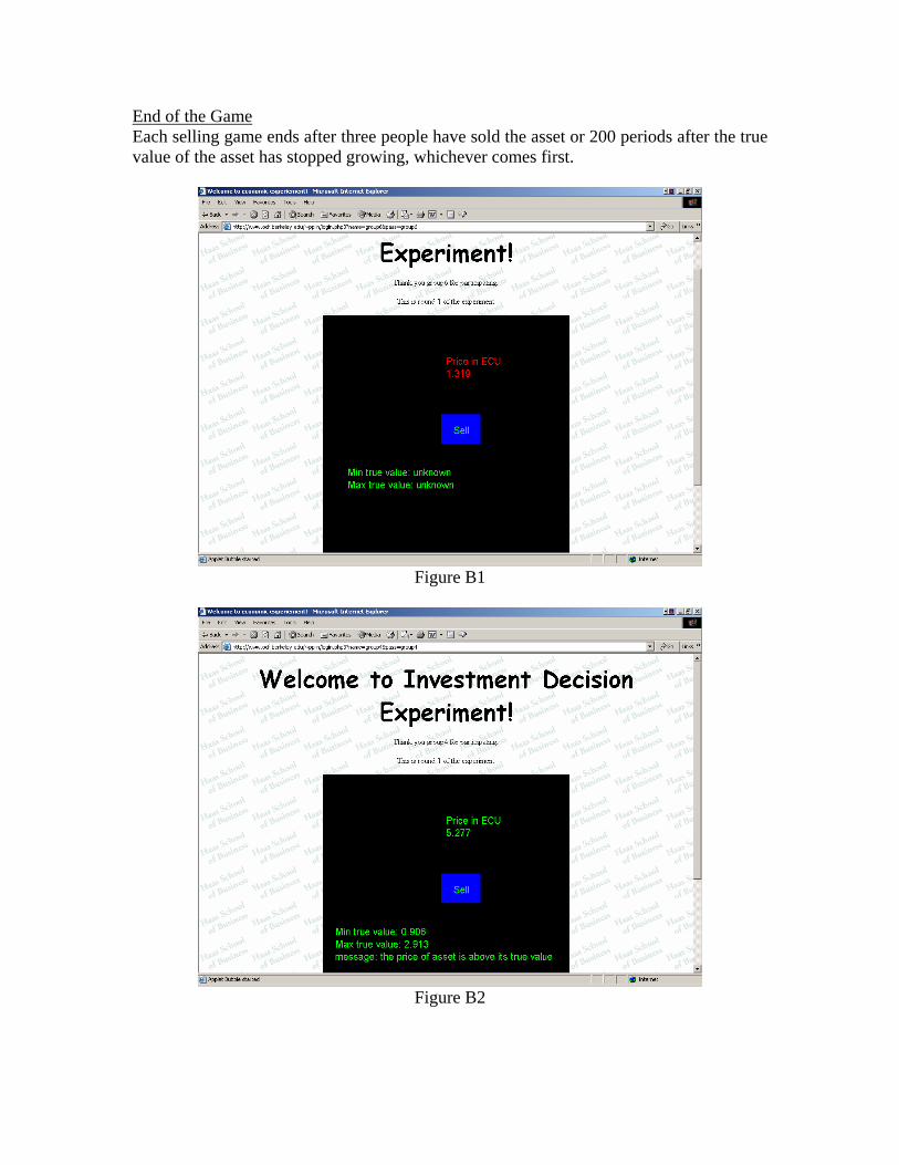
End of the Game Each selling game ends after three people have sold the asset or 200 periods after the true value of the asset has stopped growing, whichever comes first.

Figure B1

Figure B2

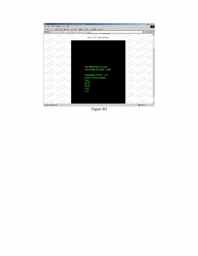
Figure B3