Clinical-Pathologic Conference: Use and choice of statistical methods for the clinical study, “Superficial adenocarcinoma of the esophagus”

The Journal of Thoracic and Cardiovascular Surgery • Volume 122, Number 6 1063

Recently, the Editor of the Journal telephoned us with a “crazy idea.”He read a few phrases from the “Patients and Methods” section ofour paper “Superficial Adenocarcinoma of the Esophagus” (whichappears in this issue1) and thought most readers would understandthe first phrase, perhaps 50% the second, maybe 10% to 25% thethird, and but a handful the fourth. His idea was to call a time-out

to bring readers up to speed on statistical methodology. He suggested we extract keyphrases from our paper and explain them in the format of a Clinical-PathologicConference (CPC).

His selection of “Superficial Adenocarcinoma of the Esophagus” is interesting,because the intensity of statistical analysis required to unlock the meaning of thedata is high. Further, the article appears in the General Thoracic Surgery section,introducing into that arena data analysis concepts and methods more frequentlyfound in the cardiac surgery sections.

Before proceeding, please read the paper.Each section of the CPC is introduced by quotations from the paper and followed

by dialogue between Drs Rice (TWR) and Blackstone (EHB). Throughout the dia-logue, key technical ideas are highlighted for discussion in marginal notes. We rec-ommend two sources of supplemental information: chapter 71 of Thoracic Surgery2

and chapter 6 of Cardiac Surgery.3

Essence of the ArticleSurgery is the treatment of choice for superficial adenocarcinoma of theesophagus. The ideal patient has high-grade dysplasia found at surveillance,good pulmonary function, and undergoes a transhiatal esophagectomy.Discovery of N1 disease or development of postoperative pulmonary compli-cations necessitating reintubation reduces the benefits of surgery. (Ultramini-Abstract)EHB: Dr Rice, for readers unfamiliar with superficial adenocarcinoma of the

esophagus, what instigated this study? TWR: Adenocarcinoma arising in Barrett esophagus is occurring with increasing

frequency, resulting in more patients presenting with cancers confined to the mucosaor submucosa—superficial adenocarcinoma. These patients are likely to be cured byoperation. Thus, my initial motivation was to provide a gold standard to which exper-imental alternatives to esophagectomy for early-stage disease could be held.

While analyzing the data and writing the manuscript, we realized that deathfrom cancer was not the primary determinant of outcome. Rather, it was comor-bidity, surgical factors, and postoperative mortality and morbidity. This

From the Department of Thoracic andCardiovascular Surgerya and the Departmentof Biostatistics and Epidemiology,b TheCleveland Clinic Foundation, Cleveland,Ohio.

Received for publication April 6, 2001; revi-sions requested May 23, 2001; revisionsreceived Aug 24, 2001; accepted for publica-tion Aug 30, 2001.

Address for reprints: Eugene H. Blackstone,MD, The Cleveland Clinic Foundation, 9500Euclid Ave, Desk F25, Cleveland, OH 44195(E-mail: [email protected]).

J Thorac Cardiovasc Surg 2001;122:1063-76

Copyright © 2001 by The AmericanAssociation for Thoracic Surgery

0022-5223/2001 $35.00 + 0 12/1/119858

doi:10.1067/mtc.2001.119858

Clinical-Pathologic Conference: Use and choiceof statistical methods for the clinical study,“Superficial adenocarcinoma of the esophagus”Eugene H. Blackstone, MDa,b

Thomas W. Rice, MDa

TXET

CPB

AH

DST

ATS

GTS

EDIT

ORI

AL

Statisticsfor theRest of Us

See related article on page 1077.

Drs Rice and Blackstone

1064 The Journal of Thoracic and Cardiovascular Surgery • December 2001

EDITO

RIAL

STATSG

TSA

HD

ETCPB

TX

Statistics for the Rest of Us Blackstone and Rice

changed the focus of the paper and enriched its clinicalapplicability.

EHB: Good long-term outcome in these patients sug-gested that the goals of treatment be surgical mortality andmorbidity approaching zero. These are goals more typical ofcoronary artery bypass grafting than cancer palliation.

Crafting a Road Map for the ReaderThe purposes of this study were to (1) evaluate theresults of surgical management of superficial adeno-carcinoma of the esophagus and (2) identify predic-tors of long-term survival for (a) decision-making(preoperative factors), (b) prognostication (operativefactors), and (c) hospital care (postoperative compli-cations). (Introduction)TWR: The statement of purpose grew out of our iterative

work with the data and results. It was not a linear processfrom hypothesis to inference. Pursuits of many leads wereabandoned. Insights gained generated new questions, whichin turn dictated new analyses, producing new insights.These are the dynamics of a serious clinical study.

EHB: When we finally understood the meaning of thedata from this iterative process, we distilled its essence intoan Ultramini-Abstract.4 From that, we developed a state-ment of purpose. The “Results” section was organized andthe “Patients and Methods” section structured in exactalignment with the statement of purpose. The words matchexactly. Thus, the paper has an explicit and consistent roadmap to guide the reader as it guided the writers.

Defining the Study GroupFrom our prospective surgical database of 577 patientsundergoing resection of esophageal carcinoma at TheCleveland Clinic Foundation beginning January 1983,122 patients were found to have superficial adenocar-cinoma of the esophagus. (Patients and Methods)TWR: It is crucial to define the study group. This may

seem simplistic, but it is not. When I came to The ClevelandClinic, I started a registry of esophageal surgery thatevolved into a prospective database. A registry preventspatients from falling through the cracks and from otherbiases of ascertainment.

EHB: Characterization of the study group includes con-text of care (the specific institution), time frame, and popu-lation from which the group was drawn.

Moving Target: Trends Across TimeThe number of patients operated on increased acrosstime. . . . The surgical technique evolved from routinethoracotomy to transhiatal esophagectomy withlymph node sampling for those patients with a lowrisk of lymph node metastases. . . . These modelsinclude factors whose prevalence changed across

Margin Notes

Ultramini-Abstract The Ultramini-Abstract was introduced to convey the essenceof a study’s findings.4 It is generally two or three sentenceslong (50 words maximum for The Journal of Thoracic andCardiovascular Surgery).

The maximum word length of the Ultramini-Abstractresulted from an experiment by the editorial office. A coupledozen manuscripts submitted to the Journal were reviewed,and 25-, 50-, 75-, and 100-word summarizing statements weregenerated and evaluated. Twenty-five words (one sentence)proved too few to capture the essence of most papers. Seventy-five words read like a condensed abstract. On occasion, theessence of a study could not be captured in 50 words. Suchmanuscripts contained too many ideas (information contentoverload); they needed to be split into two or more papers.

Although ostensibly intended for readers, an ultramini-abstract helps writers focus on the truest statements they canmake from their understanding of a study’s information, data,and analyses. It is the best preparation for writing a manuscript.

Prevalence, Incidence, RatePrevalence, incidence, and rate are used interchangeably.Perhaps common usage should prevail, because it rarely leadsto confusion. But it is not accurate. We prefer selecting the spe-cific word whose technical definition matches the context.

Prevalence is the frequency of occurrence of some factor,characteristic, event, or incident in a group. Of the three wordsbeing considered, it is the least commonly used but the mostcommonly meant! For example, Table 2 of the paper indicatesthat between 1985 and 2000 at The Cleveland Clinic, theprevalence of high-grade dysplasia among 122 patients under-going esophagectomy was 38 patients, or 31%.

Incidence is frequency of occurrence per unit of time. It isexpressed on a scale of inverse time (cases per year, deaths peryear), or rate of occurrence. The prevalence of high-grade dys-plasia in a population is governed by the rate of appearance ofnew cases (incidence) and the rate of removal of cases by death.

Rate as used in scientific contexts is a quantity per unittime. Speed is a rate: km · h–1; cardiac output is a blood flowrate: L · min–1. In the context of events, rate is synonymouswith incidence. The hazard function is a rate (deaths · year–1)and incidence. In the paper, we used hazard functions and sodid not want to confuse incidence and prevalence.

How, then, can we rephrase such common expressions asthese?

“Incidence of hospital mortality was. . . .”“Hospital mortality rate was. . . .”“Five-year survival rate was. . . .”We could write, “Prevalence of hospital mortality was. . . .”

However, in most instances, the words prevalence, incidence,and rate are superfluous. It is better to just write, “Hospitalmortality was. . . .” or “Five-year survival was. . . .”

In other contexts, the word occurrence is a suitable substi-tute for prevalence. For example, “Pneumothorax occurredin. . . .” is preferable to “Incidence of pneumothorax was. . . .”

Blackstone and Rice Statistics for the Rest of Us


TXET

CPB

AH

DST

ATS

GTS

EDIT

ORI

AL

time. Strategically, we believe that such models aredesirable and more helpful than simply attributing theimprovement in results to a so-called learning curve. . . .Because the surgical technique and decision-makingchanged across time (Appendix I) and simultaneouslyearly mortality improved (P = .01), we analyzed thepotentially confounding trends across time to identifyif possible those changes that improved results.(Patients and Methods)TWR: During the experience, marked changes occurred

in epidemiology, presentation, preoperative evaluation, sur-gical technique, and postoperative care. Does this evolutionnegate analysis of the experience? Can you identify changesthat were for better or for worse?

EHB: This was both an analytic and philosophic chal-lenge. We faced a moving target. Inferences about the rela-tion of evolutionary changes to patient outcome were notprotected by a mechanism such as a randomized clinicaltrial. If we were “good modelers,” if each change was doc-umented patient by patient, and if we had sufficient data,then multivariable analyses could quantify the impact ofchanges on outcome.5,6 That is a lot of “ifs!”

Logistic Regression for Time TrendsManagement changes were represented by dichotomousvariables (yes or no). A useful method for relating adichotomous event, such as a management change, to one ormore explanatory variables is logistic regression.

Logistic regression uses a mathematical equation knownas the logistic equation.7-9 It is a sigmoid (S-shaped) curvelike the oxygen dissociation curve (Figure 1) and thereforehas intuitive medical relevance when used in risk factor

Figure 1. Relation of an unlimited scale of risk, here expressed inlogit units, to the probability of occurrence of an event. The logis-tic equation mapping logit units to probability is shown. ln,Natural logarithm.

Sufficient DataA common misconception is that the larger the study group(called the sample because it is a sample of all such patients,past, present, and future), the larger the amount of data avail-able for analysis. However, in studies of outcome events, theeffective sample size for analysis is proportional to the numberof events that has occurred, not the size of the study group.Thus, a study of 200 patients experiencing 10 events has aneffective sample size of 10, not 200.

Ability to detect differences in outcome is coupled witheffective sample size. A statistical quantification of the abilityto detect a difference is the power of a study. This is a complexsubject, so only those few aspects of power that affect multi-variable analyses of events will be mentioned.

The rule of thumb in multivariable analysis is that the ratioof events to risk factors identified should be about 10 to 1.5,6

However, the guideline is not specific enough. Many variablesrepresent subgroups of patients, some of them few in number(such as 6 patients with T1b N1 disease). If a single patient ina small subgroup dies, multivariable analysis may identify thatsubgroup as one at high risk when, in fact, the variable repre-sents only this specific patient, not a common denominator ofrisk. The purpose of a multivariable analysis is to identify gen-eral risk factors, not individual patients experiencing events!

Thus, more than 1 event needs to be associated with everyvariable considered in the analysis. For our group, sufficientdata means at least 5 events associated with every variable.However, because variables may be correlated and subgroupsoverlap (T1b N1 patients are in the larger subgroup of N1patients as well as the T1b group), in the course of analysis, thenumber of unexplained events in a subgroup may fall below 5,which is insufficient data.

This strategy could result in identifying up to 1 factor per 5events. We get nervous at this extreme, but in small studies weare sometimes close to that ratio.

Thus, there is both an upper limit of risk factors that can beidentified by multivariable analysis and a lower limit of eventsto allow a variable to be considered in the analysis. Sufficientdata, then, implies having enough events available to test for allrelevant risk factors.

Dichotomous VariablesDichotomous variables are the simplest subset of categoricalvariables. They can take on only two different classes or values,such as yes or no, positive or negative, 0 or 1. A dichotomousoutcome may be called binary data (eg, hospital death).

Outcomes and EventsResults of therapy are outcomes. A subset of outcomes isevents. Events are expressed in analyses as dichotomous vari-ables (see above). Outcomes may be related to explanatoryvariables (see below), such as death, recurrence of cancer,functional status after surgery, or postoperative FEV1.

An outcome in one setting can be an explanatory variable inanother. In the paper, management changes were an event inthe context of examining therapy. They were explanatory vari-ables in the context of an analysis of mortality.


EDITO

RIAL

STATSG

TSA

HD

ETCPB

TX

analysis. If a risk factor imparts 2 units of risk, a robustpatient, far to the left on the graph in Figure 1, would haveonly a small probability of experiencing an event. In con-trast, a fragile patient, near 0 on the graph, would have alarge probability of experiencing the same event.10,11 In oneform or another, all types of event analyses are based on asimilar S-shaped relation.

Generally, many variables are examined in logisticregression,12,13 but for time trends, our attention was con-fined to the date of operation.

Events Occurring After Time ZeroPostoperative complications were recorded andassessed. (Patients and Methods)TWR: Outcome of cancer surgery usually is dominated

by cancer mortality. Because so few cancer deaths occurredin this study, other factors that could influence outcomewere recorded and evaluated, including events occurringduring postoperative care.

EHB: Events occurring after time zero (time ofesophagectomy in this study) generally are not analyzed aspotential risk factors. They are called time-varying covari-ables and are avoided for compelling reasons. First, becausethese events take place after time zero, some patients diebefore they occur; this affects the denominator for the analy-sis. Second, they themselves are outcomes, with their ownrisk factors that should be identified. Mortality and othercomplications following an occurrence should be studied.Third, the closer they occur to death, the more apt they areto be a surrogate for death (confounding).

We justified examining the influence of events occurringshortly after time zero as a way to gain insight into issues ofpostoperative management. Sequential analysis (discussedbelow) prevented our being fooled by confounding.

Formal, Systematic Follow-upPatients were followed up by periodic clinic visits;however, cross-sectional systematic follow-up wasmade in January 2000. (Patients and Methods) TWR: You insisted we attempt to contact all patients we

believed were still alive. Why couldn’t we depend on clinicnotes, simply recording the date patients were last seen?

EHB: Complete, “active,” systematic follow-up ofpatients is a necessity. “Passive” follow-up through clinicvisits or inquiries of patients’ physicians is inadequate.

The following hypothetical explanation may help: 100patients underwent operation on the same day. The goal wasto determine their fate 2 years later. Data were assembledfrom clinic visits. Some patients were last seen 6 monthsafter surgery, others at 10 months, a few at 15 months, and2 at 2 years. One patient died 30 months after surgery.Imagine the impossibility of obtaining a meaningful answerto the status of these 100 patients at 2 years when the status


Explanatory VariablesThe set of variables examined in relation to an outcome iscalled explanatory variables, independent variables, corre-lates, risk factors, incremental risk factors, covariables, or pre-dictors. These alternative names distinguish this set ofvariables from outcomes. No statistical properties are implied.The least understood name is independent variable (or inde-pendent risk factor). Some mistakenly believe it means thevariable is uncorrelated with any other risk factor. All it actu-ally describes is a variable that by some criterion has beenfound (1) to be associated with outcome and (2) to contributeinformation about outcome in addition to that provided byother variables considered simultaneously.

Logistic EquationThe logistic equation is P = 1/[1 + e–z], where P is probability,e is approximately 2.7183 and is known as the base for the nat-ural system of logarithms (see below), and z is the logarithmicparameter, specifically, the power to which e is raised.

The logistic equation was devised to characterize populationgrowth.7 Berkson and Hollander8 noted that it characterizeda number of biologic phenomena, including the proportion oferythrocytes lysed as their suspension medium became increas-ingly hypotonic. Berkson9 made it the basis for bioassay.

We can rearrange the logistic equation as follows:

P + Pe–z = 1ez = P/(1 – P)

z = ln(P/[1 – P])

Thus, the logistic equation relates the absolute probability, P, ofan event to an approximation of relative risk known as the oddsratio. The odds ratio is the proportion of patients experiencingan event divided by the proportion of patients not experiencingit (1 – P, the so-called complement of P): P/(1 – P). To convertthe odds ratio to a limitless scale (going from minus infinity toplus infinity), its logarithm is used, z. Dr Berkson called theunits of this scale “logit units.”10

Logistic RegressionIn the 1960s, Jerome Cornfield12,13 suggested the logarithmicodds ratio (log odds) parameter z of the logistic equation be thecarrier of explanatory variables. The mathematical form of z hesuggested was “logit linear”:

z = β∅1 + β1x1 + β2x2 + ··· + βkxk

where the β’s are regression coefficients and the x’s are riskfactors, such as age or FEV1. The β’s translate the measure-ment scale of the risk factors (x’s) onto the scale of risk (logit).

An increasing number of risk factors and a larger magnitudeof the relation between a unit change in the value of a risk fac-tor and risk “move a patient to the right” on the logit scale. Thisincrements risk commensurate with where the patient started inthe logit curve.

Since its introduction, logistic regression has become themost common form of multivariable analysis for non–time-related events such as hospital mortality, occurrence of postop-erative events, or use of particular management techniques.



TXET

CPB

AH

DST

ATS

GTS

EDIT

ORI

AL

of only 3 people was known at that time! This is callednumerators in search of denominators.14

In reality, patients undergo operations over a span oftime. One good follow-up strategy is to determine the statusof each patient at a fixed interval after surgery (as in theexample). This is the anniversary method of follow-up.15

Another good method is to ascertain the status of allpatients at a given point in time (called cross-sectional fol-low-up). This is the common closing date method, which weemployed.16 Anything short of formal, systematic, completefollow-up by one of these two methods leads to uninter-pretable survival estimates.

Descriptive StatisticsDescriptive statistics are summarized as the mean andstandard deviation for continuous variables and asfrequencies and percentages for categorical vari-ables. (Patients and Methods)TWR: Surprisingly, as a surgeon trained in technical

details, I may miss the essence of the techniques of analysisthat are introduced with this sentence. Do not be intimidatedby statistics! You need to understand the methods withoutperforming the statistics!

EHB: Nearly every phrase in this sentence has a techni-cal meaning. Each also implies assumptions about the datathat the reader is asked to take on faith!

Descriptive statistics means information that characterizesthe study group. It allows readers to appreciate the compositionof this specific group. There are often important geographicand institution referral differences in clinical studies. To avoidjumping to the conclusion, “That’s not my experience!,” read-ers should study the descriptive statistics carefully.

Ideally, patients’ data (stripped of informative identifiers)would be made available case by case. This is impractical.Instead, the study group is characterized by summarizinginformation. Summarizing information is different for dif-ferent types of variables.

Continuous VariablesSome variables, like age, can take on a different value forevery patient. This characterizes a continuous variable. Oneway to describe a continuous variable is to list each value.Cumulative distribution plots do just that. A description ofhow a cumulative distributed curve is constructed for age isgiven in the legend for Figure 2. The legend explains themedian value (50% older and 50% younger), percentiles,and quartiles.

A more abstract way to summarize age is to imagine thatthe values fall into a pattern that can be represented by abell-shaped mathematical model. Figure 3 is a histogramshowing patient age grouped into 5-year intervals. It lookssomewhat bell-shaped, like the smooth bell-shaped curvesuperimposed on it. The bell-shaped curve was constructed

Time ZeroIn time-to-event (survival) analysis, time zero is the time atwhich every patient in the study becomes at risk of experienc-ing the event being examined. In this study, time zero wasesophagectomy.

Fortunately, surgery is an unmistakable event that makeserrors of defining time zero uncommon (although they occur inparticular settings). In medical studies, time zero is often elu-sive. For example, we do not know time of onset of adenocar-cinoma of the esophagus.

Time-varying CovariablesTime-varying covariables are factors, events, or measurementswhose values change after time zero. Typical examples are res-piratory failure occurring after operation, cancer recurrence,adjuvant therapy, development of a new medical condition, andchange in blood pressure. Their proper analysis requires spe-cial mathematics. Their relation to other events, such as death,must be interpreted with care.

ConfoundingA confounder is a variable related both to outcome and togroups being compared. This presents a challenge, because it isanalogous to the researcher being required to answer the ques-tion, “Which came first, the chicken or the egg?”

Variable or Parameter?A variable is an item that can take on different values for dif-ferent patients. A parameter is a constant. The two terms areantonyms, yet they are commonly used as synonyms! We rec-ommend their proper technical usage. Thus, age is a variable,but mean age is a parameter.

Mathematical ModelA mathematical model is an equation (or set of equations) rep-resenting real data. Equations contain symbols representingparameters whose values are estimated from the data (see“Parameter Estimates,” page 1069). Mathematical models mayarise from a theory of nature or from empiric observation thatthey represent data reasonably. They are “compact” because anentire set of data is summarized by values of a small number ofparameters in the mathematical model.

Histograms and Cumulative DistributionsA histogram is a type of bar graph that summarizes the distri-bution of values of a continuous variable. Categories of thevariable are selected of equal width (eg, 5-year age groups),and the number of patients in each category is displayed on thevertical axis.

In contrast, cumulative distribution curves utilize everyvalue, not categories of values, and increment monotonicallyupward (see Figure 2). The shape of the histogram is roughlythe slope of the cumulative distribution function.


EDITO

RIAL

STATSG

TSA

HD

ETCPB

TX

from a mathematical equation called the Gaussian (normal)distribution. The Gaussian distribution equation containstwo constants that characterize its shape. These constantsare parameters. The parameter representing the locationalong the horizontal axis of the peak of the curve is calledthe mean. The estimate of the mean is average age.

The other parameter identifies the point of inflection ofthe curve on each side of the mean. This is the point of tran-sition from a steep ascent or descent to the shallower flangeof the bell. The location of the inflection point is a parame-ter called the standard deviation. The closer patient ages aregrouped together, the closer the standard deviation will be tothe mean. Ages between 1 standard deviation below themean and 1 standard deviation above it encompass 68% ofthe patients, as can be appreciated in Figure 2.

The mean and standard deviation are easily computed.But the computations are misleading if the distribution ofvalues is asymmetric (skewed). This situation may beaddressed by transformations, such as logarithms, or bynonparametric statistics, such as percentiles.

Categorical VariablesIn contrast to continuous variables, variables such as sex,depth of tumor invasion (T), and regional lymph node status(N) have values representing one of two or one of a small


Gaussian (Normal) DistributionThe equation of the bell-shaped Gaussian (normal) distributioncurve is

y = 1 e(x – µ)2

σ��2π��2σ2

where:π is a constant, approximately 3.1415927 . . ., pie is a constant, approximately 2.7183 . . ., the base of the

natural logarithmsσ is a parameter that represents the standard duration of the

variableµ is a parameter that represents the mean of the variablex represents a value of the variable X, generally graphed on

the horizontal axisy represents the probability of occurrence of a particular

value of x.Because in medicine normal has several unrelated mean-

ings, we have used the more technical term Gaussian.

Standard Deviation Versus Standard ErrorStandard deviation is the Gaussian distribution parameter rep-resenting the scatter or deviation of individual values from themean. It is a descriptive statistic.

Standard error is the standard deviation of the mean, anestimate of the precision of the mean (precision is related toscatter; accuracy is related to lack of bias—systematic devia-tion from the true value). Unlike the standard deviation, whichis similar in value for large and small samples of data, the stan-dard error decreases as n increases.

Because the Gaussian curve is symmetric around the mean,the two parameters of the Gaussian distribution are expressed bythe shorthand mean ± SD, where SD is 1 standard deviation. Thismeans 68% of patient ages fall between (mean – SD) and (mean+ SD). This is one instance, not terribly common in statistics, inwhich the shorthand ± is used instead of confidence limits.

Misleading MeansData may not be distributed symmetrically on both sides of themean. Often, they are skewed to the right (see below). The typ-ical postoperative stay may be 6 days, but a few patients stay30, 200, or more days. The presence of a few long stay valuesinflates the estimate of the mean. This typically results in astandard deviation larger in magnitude than the mean, such as10 ± 14 days. These parameter estimates imply that 68% of thestays will range from –4 days to +24 days! Yet, length of staycan take on only positive values, so –4 days alerts you to sum-marizing statistics that make no sense.

Mean and standard deviation are parameters of a specificmodel of data distribution. If the Gaussian model does not rep-resent the data well, it is a bad model, and something else mustbe done.

One thing that can be done is to transform the data onto ascale that is less susceptible to skewness. For example, the datavalues might be transformed to logarithmic scale. Logarithmsof positive numbers spread small values and bunch large ones.The mean value of logarithms may be more normally distrib-uted and have a sensible standard deviation. The mean, mean –

Figure 2. Cumulative distribution of age at operation for superfi-cial adenocarcinoma of the esophagus. Each patient’s age is rep-resented on the curve from youngest to oldest. Each unique agevalue increments to the curve by 1/n, where n is the total numberof patients. Notice that 50% of the patients were younger than 64.5years and 50% were older. This is the median age, expressed byhorizontal and vertical solid straight lines. The coarse dashedlines enclose the 25th and 75th percentiles (or quartiles), meaningthat 25% of patients were younger than the 25th percentile and75% were younger than the 75th percentile. For consistency withthe standard deviation, which encloses about 70% of the ages, the15th and 85th percentiles (15% of ages above and 15% below) areshown by fine dashed lines.



TXET

CPB

AH

DST

ATS

GTS

EDIT

ORI

AL

number of categories—hence the name categorical variable.The number of patients in each category is the frequency.Because this number varies widely from study to study, it iscustomary to express frequencies on a uniform scale,namely, the number per 100 patients (percent).

Distribution of Times to an Event (Survival Analysis)Nonparametric estimates of survival were obtained bythe method of Kaplan and Meier. The parametricmethod was used to resolve the number of phases ofinstantaneous risk of death (hazard function) and toestimate their shaping parameters (Patients andMethods). . . . The instantaneous risk of death washigh immediately after the operation, then fell to aconstant level of 4.2% per year. (Results)EHB: Nonparametric and parametric are key technical

terms. Cumulative distribution curves and histograms ofage (Figures 2 and 3) require no mathematical models con-taining parameters. They are called nonparametric statis-tics. In contrast, the bell-shaped curve superimposed on thehistogram of age (Figure 3) is an equation with parameters.

The Kaplan–Meier method produces nonparametric esti-mates of the distribution of times until death.17 It is analo-gous to the construction of Figure 2, except that, byconvention, the cumulative distribution of times until deathis turned upside down.

Figure 3. Histogram of age and superimposed Gaussian distribu-tion curve. Ages of patients have been categorized and counted in5-year intervals. The smooth curve is a parametric summary of thedistribution of age, expressed as the mean (the vertical line at thepeak of the curve) and standard deviation (enclosed by the finelydashed vertical lines). It is questionable whether the mean andstandard deviation represent the distribution of these ages well;yet the Gaussian distribution is often used in this setting becauseof tradition or ease of calculation. On the other hand, notice thatthe mean on this figure and median on Figure 2 are similar; theages enclosed within ±1 standard deviation of this figure are sim-ilar to those within the 15th and 85th percentiles of Figure 2.

SD, and mean + SD of logarithms are then raised to the powerof the base (called taking the antilogarithm), producing what iscalled the geometric mean and its asymmetric confidence lim-its. Another transformation is the inverse of each value, that is,its value divided into 1. If the inverse values are normally dis-tributed, their mean and standard deviation can be found. Then,the mean, mean – SD, and mean + SD are transformed back tothe original measurement scale, producing the harmonic meanand its asymmetric confidence limits.

An alternative is to forget about modeling the data alto-gether. Report the value for which half the patients have agreater number (median), and present various percentiles (eg,25th and 75th percentiles or 15th and 85th to be consistent withthe width of a standard duration) described in Figure 2.

SkewnessSkewness is a statistical measure of the asymmetry of distribu-tion of values for a variable. In medical data, asymmetry isoften characterized by a number of atypically large values fora variable. Because the number line proceeds from small num-bers on the left to large ones on the right, asymmetry in the datadistribution is called right skewness. (See “Misleading Means,”above.)

LogarithmA logarithm is the exponent or power of a fixed number, calledthe base. When the base is raised to that power (the antiloga-rithm), the untransformed number is regenerated. Typical basesare 10 and the number e, whose value is 2.7183 (e is called thebase of the natural logarithms). For example, the logarithms ofthe numbers 0.001, 0.01, 0.1, 1, 10, 100, and 1000 to the base10 are –3, –2, –1, 0, 1, 2, and 3.

Cumulative Distribution Versus Survival CurveIf all patients in a study have died, the distribution of timesuntil death can be depicted by a cumulative distribution func-tion, as in Figure 2. We generally are unable to use this simplecumulative distribution method because at follow-up not every-body has died.

For living patients, the time of death is not yet known; nev-ertheless, we know they have lived a specific length of timeafter time zero. Thus, we have incomplete information abouttheir length of life, not missing information. The Kaplan–Meiermethod (one of many such methods) uses both complete data(dead patients) and incomplete data (living patients) to estimateat least a portion of the distribution of time until death.

Patients with incomplete data (living) are called censored.This term comes from the way governments determine popula-tion survival from census figures, that is, by counting livingpeople.

Parameter EstimatesParameters in mathematical models are placeholders fornumeric values. When the parameters take on numeric values,the model becomes an equation that can be solved, for exam-ple, for individual patients’ risks.


EDITO

RIAL

STATSG

TSA

HD

ETCPB

TX

A parametric method using a mathematical model canalso characterize the distribution of times until death.18

Because such distributions are rarely bell-shaped, modelsmore suited to survival data are used. Raw survival data areused to estimate the parameters (constants) of these mod-els. The parametric method used in this paper was based onmathematical models of the birth–life–death process.19

Such models incorporate an expression for the rate of tran-sition from life to death, called the hazard function.18 Theyare identical to biochemical kinetics models, with reactionrate analogous to hazard function.20

In this study, the instantaneous rate of death was highimmediately after surgery, then fell rapidly to a steady valueafter about 6 months. A steady hazard (constant hazard)results in survival decreasing exponentially.

Risk factors can modulate the hazard function. In thisstudy, they raised and lowered the constant hazard rate.

Multivariable AnalysisValue of a Sequential Strategy

The strategy for the multivariable analysis used asequential approach to variables that reflects the pur-poses of the study (Methods and Materials). . . .Decision Model. . . . Prognostic Model. . . . HospitalCare Model (Results).TWR: I needed to know what elements of the data were

important during successive phases of patient care. Whatinformation is important for decision-making before aplanned operation? How is prognosis refined after esophagec-tomy by pathologic stage? What is the survival impact ofunforeseen events occurring early postoperatively?

EHB: Providing information helpful in each phase ofclinical care required a sequential approach to multivariableanalysis. Initially, only preoperative variables and their rela-tion to outcome were examined. Then, pathologic variableswere added and superceded information removed (eg,pathologic stage for clinical stage). Finally, postoperativeevents were added to the analysis.

TWR: This is a “medical” approach to multivariabledata analysis. It is an advantage to have a colleague whoknows the statistical methodology and has participated inpatient care.

ConceptsEHB: For many, multivariable analysis is a mystery. Weknow intuitively that a patient’s outcome is related to manyvariables. We measure or observe and record variables,some of which may be associated with outcome, even ifthey are not directly causal. One goal of multivariableanalysis is to identify, from among the many recorded vari-ables, those most related to outcome (risk factors).

Risk factor identification is challenging in medicine,because many variables are correlated with one another. For


Numeric values are called parameter estimates. They are esti-mates because they are based on a finite sample of data. Just as amean value (a parameter estimate) is associated with uncertaintyproportional to both the standard duration and effective samplesize, so any parameter estimate is associated with uncertainty.

Parameter values are estimated by means of statistical the-ory and procedures. The estimation process may be complex oras simple as counting and dividing (to estimate a probability).

Hazard FunctionThe hazard function is the instantaneous risk of death or othertime-related event.

If the hazard function is steady across time, it is called aconstant hazard or linearized rate. It is easily estimated bydividing the number of events by the total of follow-up time forthat event. A constant hazard results in survival decreasingexponentially. This is analogous to exponential radioactivedecay driven at a constant rate, called the half-life.

In most medical settings, the hazard function is not con-stant. The human population hazard function is high at birth,diminishes rapidly, is relatively flat for a few decades, and thenrises with advanced age (sometimes called a bathtub-shapedhazard function).

The units of hazard are inverse time. Because it is instanta-neous, the magnitude of the hazard function can be huge for ashort while, such as immediately after surgery. If the durationof high hazard is brief, few deaths will ensue, however.

Multivariable Versus MultivariateMultivariable analysis is an analysis of a set of explanatory vari-ables with respect to a single outcome variable. Multivariateanalysis is an analysis of several outcome variables simultane-ously with respect to explanatory variables.

Before modern multivariate analysis was possible, the termsmost used for a multivariable analysis were “multiple” or “mul-tivariate.” Since the advent of methods to analyze multiple out-comes simultaneously, multivariable has come to be associatedwith simple outcomes analysis in the American literature.European literature groups these together as multivariate, per-haps because multivariable analysis is the degenerate form ofmultivariable analysis when number of outcomes is 1.

Strength of AssociationThe strength of association of a risk factor with outcome isexpressed by a type of parameter called a coefficient. A coeffi-cient is a multiplier in an algebraic expression. For example, inthe expression 0.026 × age, 0.026 is the coefficient and multi-plier of age. The coefficient translates units of age into units ofage-associated risk.

Most multivariable models consist of an additive relationamong risk factors, as shown for logistic regression. That is,each variable in the analysis, such as age, FEV1, or type of can-cer, is weighted by its coefficient (generally, the larger theweight, the stronger the association with outcome). Then, theproduct pairs of the coefficient and variable are added togetherwith all other pairs to form a risk score.

can lead to restrictive prespecifying of variables to be exam-ined, which may preclude generation of new knowledge.

Organizing VariablesThe potential risk factors (variables) were organizedfor analysis. . . . (Patients and Methods)TWR: The key to your analyses is grouping similar risk

factors. Is this a more powerful strategy than consideringeach factor as it appears in an unordered list?

EHB: Organization of well-understood, high-qualityvariables is key to successful, medically informed model-ing of outcomes. To the casual statistical consultant, allvariables are equal. Under such circumstances, chances arereduced that the analyses will “turn out right.” In a collab-orative effort, those analyzing the data become familiarwith each variable, what it means, how its values weregathered, its quality in terms of accuracy and precision,and other knowledge and understanding of the variables,patients, and goals of the study. From this intimate knowl-edge of the variables, we group them into medically mean-ingful classes.

We consider the class of variables as “the” variable andthe individual variables within the class as minor differencesin specification. To illustrate, we consider “patient size” asthe variable, but it may be represented by height, weight,body surface area, or body mass index.



TXET

CPB

AH

DST

ATS

GTS

EDIT

ORI

AL

example, women on average are shorter and have a smallerbody surface area than men; sex, height, and body surfaceare correlated. Risk factors are identified in a context thataccounts for correlated information by evaluating all vari-ables simultaneously. The strength of association with out-come of each variable is adjusted for all other variables inthe analysis. Thus, it is correct to think of this strength as theincremental risk the variable adds beyond that contributedby all other simultaneously considered variables.

The number of variables that can be in a model simulta-neously is limited by the number of events, not total n. (See“Sufficient Data.”) Thus, although we might like to considerall variables at once and then trim down the list (called abackward variable selection strategy), in this study, with alimited number of events, we built the model gradually fromsimple (few variables) to more complex (greater number ofvariables) using a forward variable selection strategy.

When the number of events is small, we recommenddeveloping a parsimonious multivariable model (the sim-plest model that adequately explains the data).19 Thus, theanalysis is directed toward finding the common denomina-tors of the event.3

Understanding the VariablesInitial screening of variables possibly related to sur-vival used the log-rank test and the Cox proportionalhazards model. (Patients and Methods)TWR: Because many factors influence patient survival,

it is necessary to use multivariable analysis. So what good isscreening variables one at a time and presenting univariableresults?

EHB: We screen individual variables to answer a coupleof questions. First, are there sufficient data for analysis? Asnoted earlier, if there are fewer than about 5 events associ-ated with a subgroup of patients, we cannot use this sub-group for multivariable analysis. Second, is there aproportional hazards relationship between a variable andoutcome? By proportional hazards, we mean the ratio ofhazard when a risk factor is present to that when it is absentis constant across time. This assumption of Cox propor-tional hazards modeling must be verified if that method ofrisk factor analysis will be used.21

Truthfully, other than “weeding out” variables and test-ing assumptions, I pay little attention to univariable survivaltests. What is important is the multivariable relations. Thus,I do not prescreen to get rid of otherwise perfectly good butnot univariably statistically significant variables. There areinstances in which the relation of a variable to outcome ishidden in univariable analyses, and not until other factorshave been accounted for is it revealed. These are called lurk-ing variables.22

A controversial use of screening is to restrict the numberof variables examined in the multivariable analysis.23 This

Checking the Proportional Hazards AssumptionWhenever Cox proportional hazards analysis is performed, theassumption of proportional hazards must be verified. The Coxmodel is formulated for a single dichotomous variable as follows:

Λ(t) = Λ0(t)eβ1x1

where Λ(t) is the cumulative hazard function, Λ0(t) is theunderlying cumulative hazard (not specified explicitly), e is2.7183. . ., the base of the natural logarithm, β1 is the Coxregression coefficient, and x1 is the dichotomous variable.

The ratio of cumulative hazard with the factor present (x1 =1) to that with it absent (x1 = 0) is

Λ(t,x1 = 1) = eβ1

Λ(t,x1 = 0)

Taking logarithms:

β1 = ln[Λ(t,x1 = 1)] – ln[Λ(t,x1 = 0)]

Notice that the logarithm of the two cumulative hazard curvesis separated across all time by β1. If separation is not constant,the proportional hazards assumption is violated.

Cumulative hazard is estimated from the survival curve S(t)by taking the logarithm:

Λ(t) = – ln[S(t)]


EDITO

RIAL

STATSG

TSA

HD

ETCPB

TX

CalibrationContinuous and ordinal variables were assessed uni-variably by decile risk analysis to suggest transfor-mations of scale to incorporate into the multivariableanalyses to ensure that the relation of these variablesto outcome was well calibrated with respect to modelassumptions. (Patients and Methods)TWR: Many investigators stratify continuous variables

into two (or a few) groups and analyze the resulting cate-gories. I notice that you always analyze continuous vari-ables as such. Is this just a difference in style?

EHB: Continuous variables contain information unique toeach patient. Creating categorical variables from continuousvariables wastes precious information. Generally, the cut points(points of categorization, such as age > 70 years) are arbitrary.This practice flies in the teeth of a philosophical idea: continu-ity in nature.19 A 69.9-year-old is more like a 70.1-year-old thana 59-year-old or an 85-year-old. We nearly always find that con-tinuously valued risk factors follow a smooth gradient of riskthat supports the idea of continuity in nature.

There is a scientific argument as well. We are interestedin knowing the shape of the relationship of the variable tooutcome. You cannot characterize the shape if you begin bycategorizing continuous variables.

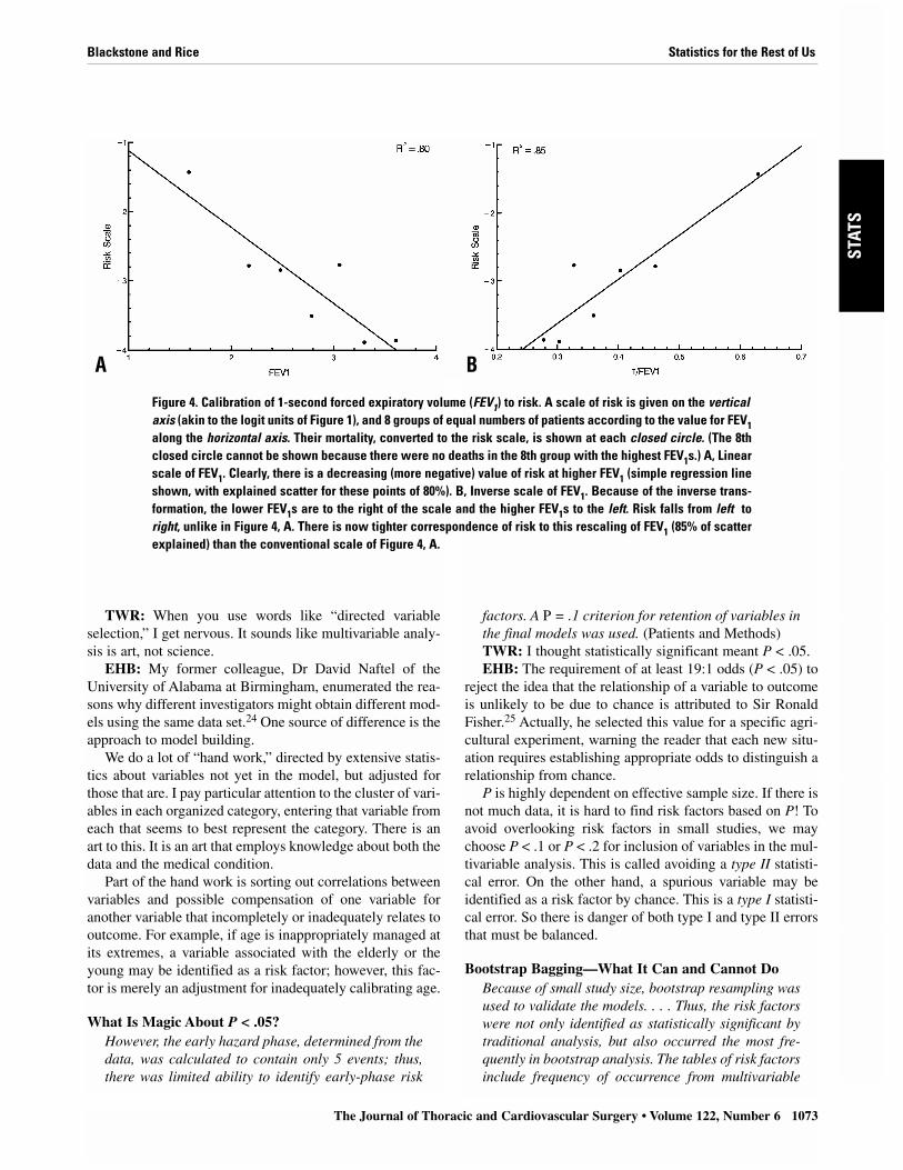
TWR: I remember your asking me, “At what value isFEV1 [1-second forced expiratory volume] associated withreduced survival?” I said, “About 2 L.” As plotted in thepaper’s Figure 5, this is indeed the case. However, this rela-

tionship is not continuous. It is flat to about 2.2 L; then it isassociated with decreasing survival.

EHB: This particular shape was suggested by a calibra-tion process that took the form of linearizing transforma-tions. Figure 4, A, shows a scale of risk along the vertical axisand FEV1 on the horizontal axis. The relation of FEV1 to thescale of risk is not perfectly linear. Figure 4, B, shows a trans-formed scale FEV1, and the points now line up straighter.This is what is meant by a linearizing transformation.

When we “unwound” the transformation for FEV1, itbecame evident that above about 2.2 L there was littleincrement in risk and below it, a substantial and steep gra-dient of risk. Thus, we had discovered the shape of therelationship.

Managing Missing Values for VariablesInformative imputation for missing values of pul-monary function tests used a multiple regressionmodel based on available function tests, age, and sex.(Patients and Methods)TWR: A number of patients did not have pulmonary

function tested preoperatively. If these patients were dis-carded, their other data would be wasted.

EHB: Most investigations of missing data have been insocial science, where it makes sense to discard from analy-sis individuals who fail to return their survey. Less attentionhas been given to sporadic missing data, characteristic ofclinical studies.

For sporadic missing data, we usually impute (substitute)the mean value of patients with nonmissing data. We verifythe imputed data are noninformative (that is, they do not addinformation that biases the results of analysis) by formingindicator variables. These identify patients in whom valuesfor a particular variable have been imputed. The indicatorvariables are incorporated into analyses to test whetherpatients with missing data behave differently with respect tooutcome than patients with available data.

In the case of pulmonary function tests in this study,more than a small amount of data was missing. Therefore,knowing that medical data contain correlated variables, weperformed informative imputation. Specifically, we substi-tuted a value based on other variables correlated with pul-monary function, rather than the mean for the whole group.To do this, we performed a multivariable analysis of pul-monary function tests from patients with nonmissing mea-surements. This generated an equation to predict pulmonaryfunction of those patients based on age and sex.23

Identifying the Risk FactorsMultivariable survival analysis was performed foreach hazard phase using a directed technique of entryof variables into the multivariable models. (Patientsand Methods)


Accuracy Versus PrecisionAccuracy is the absence of systematic error of measurement(bias) from the “truth.” Precision is the ability to provide thesame answer in repeated measurements. These terms are com-monly interchanged, but in data analysis they are different.Scales may be inaccurate because of an offset of weight orincorrect calibration. However, they may yield repeatable (pre-cise), inaccurate readings. A measurement may be imprecisebecause of inability to obtain consistent results, because thescale may be too coarse, or because of interobserver error.

Linearizing TransformationsTo linearize the relation between the measurement scale of acontinuous or ordinal variable and the scale of risk may requiretransformation of the measurement scale. Transformations ofscale might include inverse, logarithm, power, root (such assquare root), and so on. The right transformation produces ascale linearly related to risk.

Other techniques can be used to ensure a linear relationshipbetween risk and measurement scales that, together, we callcalibration. Calibration is extra work! Busy statisticians maynot be given (or take) the time necessary to explore calibration.It is worth the time!

factors. A P = .1 criterion for retention of variables inthe final models was used. (Patients and Methods)TWR: I thought statistically significant meant P < .05.EHB: The requirement of at least 19:1 odds (P < .05) to

reject the idea that the relationship of a variable to outcomeis unlikely to be due to chance is attributed to Sir RonaldFisher.25 Actually, he selected this value for a specific agri-cultural experiment, warning the reader that each new situ-ation requires establishing appropriate odds to distinguish arelationship from chance.

P is highly dependent on effective sample size. If there isnot much data, it is hard to find risk factors based on P! Toavoid overlooking risk factors in small studies, we maychoose P < .1 or P < .2 for inclusion of variables in the mul-tivariable analysis. This is called avoiding a type II statisti-cal error. On the other hand, a spurious variable may beidentified as a risk factor by chance. This is a type I statisti-cal error. So there is danger of both type I and type II errorsthat must be balanced.

Bootstrap Bagging—What It Can and Cannot DoBecause of small study size, bootstrap resampling wasused to validate the models. . . . Thus, the risk factorswere not only identified as statistically significant bytraditional analysis, but also occurred the most fre-quently in bootstrap analysis. The tables of risk factorsinclude frequency of occurrence from multivariable



TXET

CPB

AH

DST

ATS

GTS

EDIT

ORI

AL

TWR: When you use words like “directed variableselection,” I get nervous. It sounds like multivariable analy-sis is art, not science.

EHB: My former colleague, Dr David Naftel of theUniversity of Alabama at Birmingham, enumerated the rea-sons why different investigators might obtain different mod-els using the same data set.24 One source of difference is theapproach to model building.

We do a lot of “hand work,” directed by extensive statis-tics about variables not yet in the model, but adjusted forthose that are. I pay particular attention to the cluster of vari-ables in each organized category, entering that variable fromeach that seems to best represent the category. There is anart to this. It is an art that employs knowledge about both thedata and the medical condition.

Part of the hand work is sorting out correlations betweenvariables and possible compensation of one variable foranother variable that incompletely or inadequately relates tooutcome. For example, if age is inappropriately managed atits extremes, a variable associated with the elderly or theyoung may be identified as a risk factor; however, this fac-tor is merely an adjustment for inadequately calibrating age.

What Is Magic About P < .05?However, the early hazard phase, determined from thedata, was calculated to contain only 5 events; thus,there was limited ability to identify early-phase risk

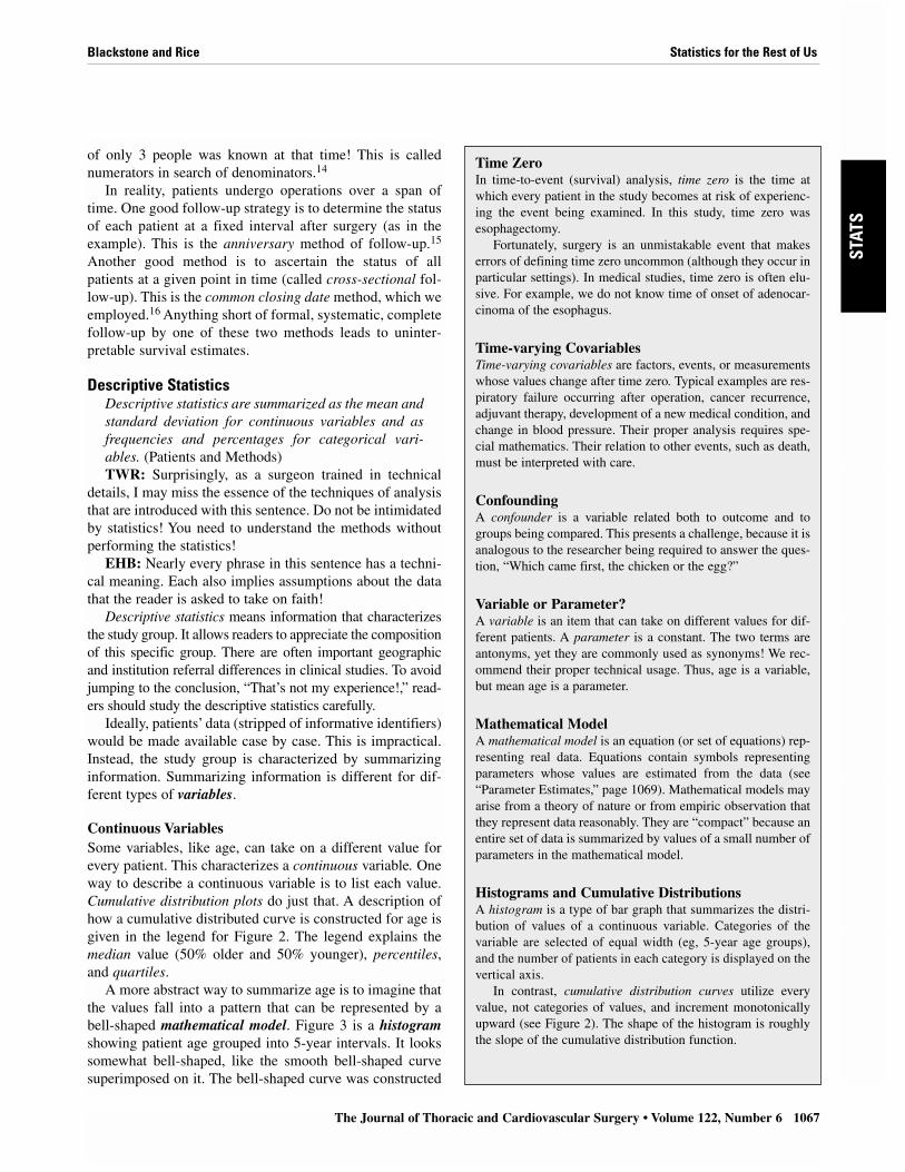
Figure 4. Calibration of 1-second forced expiratory volume (FEV1) to risk. A scale of risk is given on the verticalaxis (akin to the logit units of Figure 1), and 8 groups of equal numbers of patients according to the value for FEV1along the horizontal axis. Their mortality, converted to the risk scale, is shown at each closed circle. (The 8thclosed circle cannot be shown because there were no deaths in the 8th group with the highest FEV1s.) A, Linearscale of FEV1. Clearly, there is a decreasing (more negative) value of risk at higher FEV1 (simple regression lineshown, with explained scatter for these points of 80%). B, Inverse scale of FEV1. Because of the inverse trans-formation, the lower FEV1s are to the right of the scale and the higher FEV1s to the left. Risk falls from left toright, unlike in Figure 4, A. There is now tighter correspondence of risk to this rescaling of FEV1 (85% of scatterexplained) than the conventional scale of Figure 4, A.

A B


EDITO

RIAL

STATSG

TSA

HD

ETCPB

TX

bootstrap modeling, as well as conventional magni-tude and certainty of the association. (Patients andMethods)TWR: When you introduced me to bootstrapping, my

hope was that it would multiply the data, eliminating thelimitation of n. That is not how it works, and its role is dif-ferent.

EHB: Actually, it is the proverbial answer to themaiden’s prayer, but a different prayer than you had hopedfor! Remember the dilemma that using P value criteriaexposes the investigator to the chance of both spurious riskfactor detection and failure to detect? Remember your accu-sation of “art, not science” in variable selection?

Recently, a technique has been introduced that is similarin concept to visual evoked potentials or signal-averagedelectrocardiograms.26 The entire analytic process of variableselection is subjected to repeated resampling and reanalysis.

In practice, a patient is drawn at random (using a randomnumber generator) from the original data set. This beginsthe formation of a new data set. Another patient is drawn atrandom; it might be the same patient or a different one. Thisgoes on until a new data set is built with either the samenumber of observations as the original or somewhat fewer.An automated process is then used to select variables. Oncea model is obtained, it is stored in the computer. This entireprocess of selecting patients and performing an analysis isrepeated 100 to 1000 times. As the results are averaged, a“signal” gradually emerges.27 Some variables are repeatedlyfound to be risk factors, others only occasionally. The fewthat stand out as consistent are reliable risk factors.28

Let me try to put this process into your domain. Imagine aspace alien trying to figure out what a thoracic surgeon is. Ifthe alien watches randomly throughout the day, it may find thesurgeon asleep, eating, playing baseball with children, exam-ining a patient, or performing an operation in the thorax. Afterrepeated examinations of a randomly selected group of tho-racic surgeons, the picture gradually emerges that this is a per-son who performs operations for diseases of the lungs,esophagus, and chest wall. If the alien is observing differencesbetween thoracic surgeons and people at random, factors likesleeping and eating and playing with children disappear intothe background and the professional profile emerges.

Presenting ResultsConfidence Limits: Expressing Uncertainty ofInferences

Confidence limits (CL) of proportions are also equiv-alent to 1 standard error (68% CL) (Patients andMethods). . . . Two patients died in the hospital afterthe operation and 1 within 30 days, for an operativemortality of 2.5% (CL 1.1%-4.9%). (Results)TWR: You and Dr John Kirklin introduced confidence

limits into our literature in the late 1960s. I have not seen

many papers recently that utilize them as extensively as yousuggested.

EHB: Their need and utility are as compelling today as30 years ago. There were 2 deaths in the hospital and 1 outof the hospital within 30 days in your study. The fact is thatmortality was 2.5%. There is nothing uncertain about this.However, confidence limits translate an experience of thepast into an estimate of results in future patients. Intuitively,the smaller the experience, the less certainty that results willbe similar in the future. In this experience, 2.5% mortality(called the point estimate) is consistent with mortality rang-ing from about 1% to 5%.

I do not know why surgeons have not found this infor-mation useful. Even the general public expects pollsters togive them a “margin of error.”

Multivariable ResultsTables of risk factors identified in the hazard domainare presented with their regression coefficients ratherthan hazard ratio, because the model is not one ofproportional hazards. (Patients and Methods)TWR: Some years ago you used bullets to indicate risk

factors and possibly a P. Now you use complex tables withmultiple footnotes. In addition, I am accustomed to obtain-ing hazard ratios from our statistician, but you give meregression coefficients. Why?

EHB: A multivariable analysis generates an enormousamount of information about (1) the model’s structure andestimates of model structural parameters (if one is usingparametric modeling); (2) risk factors identified; (3) magni-tude of the association of risk factors with outcome(expressed as coefficients, odds ratios, or hazard ratios); (4)direction of relation (positive, negative); (5) uncertainty ofassociation (standard deviation); (6) score on which P isbased; (7) P; (8) covariance structure (documenting interre-lations among variables); and recently, (9) bootstrap relia-bility. There is no room to print all of this information!Therefore, some triage is nearly always necessary (a com-plete transcription of a multivariable model is also some-times needed28); bullet points were one approach to triage.

As to why we do not use hazard ratios, the answer issimpler. Hazard ratios are meaningful under assumptions ofproportional hazards. When we use transformations of scaleand nonproportional hazards modeling, hazard ratios are notreadily interpretable.

A Picture Is Worth 1000 Words. . . because the hazard function multivariable analy-ses are completely parametric (generate an equation),“nomograms” from the analyses are presented inwhich specific values are entered into the equations,the equations solved, and the results presented graph-ically with confidence limits. (Patients and Methods)




TXET

CPB

AH

DST

ATS

GTS

EDIT

ORI

AL

TWR: The value of a parametric analysis is that it pro-duces an equation that can be solved for any patient withany risk factor. It is about more than just identifying riskfactors.

EHB: The solution, moreover, can be presented graph-ically in what we call nomograms. This was one of themotivations for our developing a completely parametrichazard function methodology.18 Thus, I can show you therelationship of survival and FEV1, or of survival and age,by solving an equation. I can plot a graph of a patient’sspecific prognosis from the equation.29 This informationis ideal for understanding disease and its treatment, formaking individual patient decisions, and for obtaininginformed consent.

Nomograms require only simple high school level alge-bra. Values for all variables in the model are multiplied bytheir respective coefficients, the products are summed, therest of the equation is solved, and a plot is generated.

Internal Verification of Model AdequacyThe accuracy of this model is corroborated by thecomparison to actual deaths (Results). . . . Adequacyof the prognostic model (Table 5)TWR: If a person has pN1 disease, prognosis is grim.

Increasing depth of tumor invasion is also related to poorersurvival, by univariable analysis. However, depth of tumorinvasion (T) is related to the probability of having N1 dis-ease.30 Yet I do not see T in the prognostic model. Why not?

EHB: Patients with greater depth of tumor invasion havepoorer survival that those with more superficial disease.However, greater tumor invasion is accompanied by othereven more prognostically important factors, such as pN1disease. After accounting for other factors, depth of tumorinvasion contributed too little additional prognostic infor-mation to be retained in the multivariable model.

It is possible that small effective sample size precludeddetecting an additional increment of risk related to T or thatthe study was too restrictive in the spectrum of T (confinedto superficial carcinomas) to detect a more general trend ofincreasing risk with increasing depth of invasion. One of thebeauties of a completely parametric model is that we cancheck this out! Using the multivariable model (see “Patient-specific Prediction”), we calculated expected survival foreach level of tumor invasion.

As Appendix Figure I (paper) shows, there was good cor-respondence with Kaplan–Meier survival estimates strati-fied by T. Even though T was not directly represented in themodel, it was adequately accounted for by other variables,such as pN1.

It would be a mistake to conclude that T is not a risk fac-tor. Certainly, the greater the depth of tumor invasion, theworse the survival. However, the poorer prognosis isaccounted for by other factors correlated with T.

Interpreting Results: Importance of an ExternalStandard

After accounting for pathologic stage, age at opera-tion became a risk factor. No sharp age cutoff wasidentified: the older the patient, the shorter the sur-vival. However, patients younger than 55 years hadpoorer survival than their US population counter-parts, whereas patients aged 55 to 75 and those morethan 75 years lived about as long as expected.(Results)TWR: Before you started the analysis, I believed that we

should not be operating on older patients. You changed mymind. Certainly, older patients have a more complex hospi-tal course and poorer survival than younger patients, as youshow in the multivariable model. You have convinced methat the prognosis of older patients is better and the progno-sis of younger patients is actually worse. Explain this.

EHB: The problem with age is that it is a risk factor formortality for all of us. So I inquired whether the relationof advanced age to survival was different after surgeryfrom that expected in the general population. I used gov-ernment life tables to construct a survival curve for eachpatient based on age, sex, and ethnicity. These curves werethen averaged within age groups for convenience of com-parison.

Although elderly patients had an increased early mortal-ity, overall they fared about as well as predicted for the gen-

Patient-specific PredictionParametric models permit the calculation of patient-specificsurvival curves as in Figure 6 (paper).3 These curves can begenerated for alternative treatments and compared with thatactually given.29

Perhaps unappreciated is that a multivariable analysisreveals differences in survival unsuspected by average survivalexpressed by Kaplan–Meier curves. In Figure 6 (paper), thelow-risk and high-risk patient-specific predictions are quite dif-ferent. Both differ substantially from the average Kaplan–Meier curve. This is why we should calculate individual sur-vival probabilities on the basis of information we know.

Patient-specific predictions also have a role in interval vali-dation of model accuracy. We use two methods. First, at theactual time of follow-up or death for each patient, we calculatepredicted survival. Survival is transformed to cumulative haz-ard. The sum of cumulative hazards across patients will equalthe number of events observed. We then subgroup patients andverify that the number of predicted deaths is similar to thenumber observed in each subgroup.

Another way to verify a model is to generate a patient-specificsurvival curve for each patient. The patients are then subgrouped.We verify that the average of these individual curves correspondsto actual subgroup Kaplan–Meier survival estimates.


EDITO

RIAL

STATSG

TSA

HD

ETCPB

TX

eral population. Younger patients had a distinctly worseprognosis than their counterparts in the general population,even though their survival after surgery was better than forolder patients.

EHB and TWR: EpilogueThis CPC illustrates important facets of clinical investiga-tion. It shows that collaboration between the clinical inves-tigator and analyzers of the data is crucial. The knowledgeof these individuals is not mutually exclusive, but shared.This facilitates a clinically pertinent data analysis and pre-sentation that has clinical inferences for future patient care.It also leads to questions for further investigation. Finally, itmaximizes the extraction of useful information from thedata. However, this requires application of ever-changingtechnology in data analysis, statistics, and informatics.

References1. Rice TW, Blackstone EH, Goldblum JR, DeCamp MM, Murthy SC,

Falk GW, et al. Superficial adenocarcinoma of the esophagus. JThorac Cardiovasc Surg. 2001;122:1077-90.

2. Piantadosi S, Kirklin J, Blackstone E. Statistical terminology and def-initions. In: Pearson FG, Deslauriers J, Ginsberg RJ, Hiebert CA,McKneally MF, Urschel HC Jr, editors. Thoracic surgery. New York:Churchill Livingstone; 1995. p. 1649-77.

3. Kirklin JW, Barratt-Boyes BG. Generation of knowledge from infor-mation, data and analyses. In: Cardiac surgery, Vol 1, 2nd ed. NewYork: Churchill Livingstone; 1993. p. 249-82.

4. Kirklin JW, Blackstone EH. Notes from the Editors: Ultramini-abstracts and abstracts. J Thorac Cardiovasc Surg. 1994;107:326.

5. Harrell FE Jr, Lee KL, Califf RM, Pryor DB, Rosati RA. Regressionmodelling strategies for improved prognostic prediction. Stat Med.1984;3:143-52.

6. Marshall G, Grover FL, Henderson WG, Hammermeister KE.Assessment of predictive models for binary outcomes: an empiricalapproach using operative death from cardiac surgery. Stat Med.1994;13:1501-11.

7. Verhurst PF. Notice sur la loi que la population suit dans son accroisse-ment. Math Physique. 1838;10:113-21.

8. Berkson J, Hollander F. On the equation for the reaction betweeninvertase and sucrose. J Wash Acad Sci. 1930;20:157-72.

9. Berkson J. Application of the logistic function to bio-assay. J Am StatAssoc. 1944;39:357-65.

10. Berkson J. Why I prefer logits to probits. Biometrics. 1951;7:327-39.

11. Kirklin JW. A letter to Helen (presidential address). J ThoracCardiovasc Surg. 1979;78:643-54.

12. Cornfield J. Joint dependence of risk of coronary heart disease onserum cholesterol and systolic blood pressure: a discriminant functionanalysis. Fed Proc. 1962;21:58-61.

13. Gordon T. Statistics in a prospective study: the Framingham study. In:Gail MH, Johnson NL, coordinators. Proceedings of the AmericanStatistical Association: Sesquicentennial Invited Paper Sessions.Alexandria (VA): American Statistical Association; 1989. p. 719-26.

14. Spodick DH. Numerators without denominators: there is no FDA forthe surgeon. JAMA. 1975;232:35-8.

15. Drolette M. The effect of incomplete follow-up. Biometrics. 1975;31:135-44.

16. Elveback L. Estimation of survivorship in chronic disease: the “actu-arial” method. J Am Stat Assoc. 1958;53:420-40.

17. Kaplan EL, Meier P. Nonparametric estimation from incompleteobservations. J Am Stat Assoc. 1958;53:457-81.

18. Blackstone EH, Naftel DC, Turner ME Jr. The decomposition of time-varying hazard into phases, each incorporating a separate stream ofconcomitant information. J Am Stat Assoc. 1986;81:615-24.

19. Blackstone EH. Black death, smallpox, and continuity in nature:philosophies in generating new knowledge from clinical experiences.Thorac Cardiovasc Surg. 1999;47:279-87.

20. Blackstone EH. Outcome analysis using hazard function methodol-ogy. Ann Thorac Surg. 1996;61:S2-7.

21. Cox DR, Oakes D. Analysis of survival data. London: Chapman andHall; 1984.

22. Joiner B. Lurking variables: some examples. Am Stat. 1981;35:227-33.

23. Harrell FE Jr, Lee KL, Mark DB. Tutorial in biostatistics: multivari-able prognostic models—issues in developing models, evaluatingassumption and adequacy, and measuring and reducing errors. StatMed. 1996;15:361-87.

24. Naftel DC. Do different investigators sometimes produce differentmultivariable equations from the same data? J Thorac CardiovascSurg. 1994;107:1528-9.

25. Fisher RA. Statistical methods and scientific inference. Edinburgh:Oliver and Boyd; 1956, p. 42.

26. Breiman L. Bagging predictors. Machine Learning. 1996;26:123-40.27. Blackstone EH. Breaking down barriers: helpful breakthrough statisti-

cal methods you need to understand better. J Thorac Cardiovasc Surg.2001;122:430-9.

28. Piehler JM, Blackstone EH, Bailey KR, Sullivan ME, Pluth JR, WeissNS, et al. Reoperation on prosthetic heart valves. J Thorac CardiovascSurg. 1995;109:30-48.

29. Lytle BW, Blackstone EH, Loop FD, Houghtaling PL, Arnold JH,Akhrass R, et al. Two internal thoracic artery grafts are better than one.J Thorac Cardiovasc Surg. 1999;117:855-72.

30. Rice TW, Zuccaro G Jr, Adelstein DJ, Rybicki LA, Blackstone EH,Goldblum JR. Esophageal carcinoma: depth of tumor invasion is predic-tive of regional lymph node status. Ann Thorac Surg. 1998;65:787-92.


Documents

Clinical-Pathologic Conference: Use and choice of statistical methods for the clinical study, “Superficial adenocarcinoma of the esophagus”