Estimation of Water Demand in Developing Countries: An Overview

Céline Nauges

Dale Whittington

Abstract

A better understanding of household water use in less developed countries (LDCs) is

necessary to manage and expand water systems more effectively. Several meta-analyses have

examined the determinants of household water demand in industrialized countries, but little

effort has been made to synthesize the growing body of literature evaluating household water

demand in LDCs. This article reviews what is known and what is missing from that literature

thus far. Analysis of demand for water in LDCs is complicated by abundant evidence that,

contrary to what is observed in most developed countries, households in LDCs have access to

and may use more than one of several types of water sources. We describe the different

modeling strategies that researchers have adopted to estimate water demand in LDCs, and

discuss issues related to data collection. The findings from the literature on the main

determinants of water demand in LDCs suggest that despite heterogeneity in places and time

periods studied, most estimates of own price elasticity of water from private connections are

in the range of –0.3 to –0.6, close to what is usually reported for industrialized countries. The

empirical findings on household water source decisions are much less robust and should be a

high priority for future research.

1

2

Introduction

This article reviews what is known and what is missing from the growing body of

literature on household water demand functions in less developed countries (LDCs). We also

discuss the challenges researchers face in carrying out studies of household water demand in

the constrained data environment of developing countries, and how these can be overcome.

Studies of residential water demand in industrialized countries have mainly concerned

measurement of price and income elasticities. In these countries almost all households have a

connection to the piped water network, and tap water, generally of good quality, is the

primary source for all water uses. These characteristics permit a relatively straightforward

estimation of the household water demand function. The chief methodological issue that has

been extensively discussed in this literature is the nonlinearity of the pricing scheme, which

may cause endogeneity bias at the estimation stage.

Analyses of household water demand in LDCs first appeared in the work of White and

others (1972), Katzman (1977), and Hubbell (1977) but remain limited even today. One

reason for this lack of attention is that analyses of household water demand in LDCs are more

difficult to do. This is mainly because conditions surrounding water access often vary across

households, and this variability makes it almost impossible to base a comprehensive analysis

of household water demand on secondary data from the water utility. Households often rely

on a variety of water sources, including piped and nonpiped sources with different

characteristics and levels of services (price, distance to the source, quality, reliability, etc.).

For many households in LDCs water is a heterogeneous good, which is not usually the case in

industrialized countries (Mu and others 1990). Obtaining water from nontap sources outside

the house involves collection costs that need to be taken into account to assess household

behavior accurately.

Researchers have employed four principal strategies to obtain the information needed

to investigate household water demand behavior in LDCs. First, well-designed household

surveys can be used to complement existing data from public (and private) utilities.1 Second,

households can be asked questions about how they would behave in hypothetical water use

situations (e.g., Whittington and others 1990a; The World Bank Water Demand Research

Team 1993 and Whittington and others 2002). Third, researchers can look to secondary

markets such as housing to draw inferences about how households value improved water

services (e.g., North and Griffin 1993, Daniere 1994, and, for a review, Komives 2003).

Fourth, experimental methods (including randomized controlled trials) can be used to test how

households behave in response to different water supply interventions (Kremer and others

2007, 2008).

This paper reviews the literature that uses data from utilities and household surveys to

estimate household water demand functions, not papers that investigate water demand

behavior based on stated preference techniques, revealed preference techniques, or

experimental methods. We begin with an overview of three large groups of households in

LDCs and discuss why water planners need somewhat different information about household

water demand behavior to address the policy challenges each household group poses. We then

provide a brief overview of the literature on the estimation of water demand functions in

industrialized countries because research based on data from LDCs has been informed by

findings from this work. Methodologies developed to correct for price endogeneity under

nonlinear pricing have in particular been applied in recent studies of household water demand

functions in LDCs.

Next we describe the different modeling strategies that researchers have adopted to

estimate water demand functions in LDCs, and discuss issues related to data collection. We

then review the findings from the literature on the main determinants of water demand

3

functions in LDCs: water price, cost of water collection, quality of water service, and

household socioeconomic characteristics. In our conclusions we discuss the policy

implications of the findings from this literature and indicate directions for future research. In

the Appendix we offer some recommendations for the design of household surveys that

collect data to estimate water demand functions.

Background

Broadly speaking, there are three large groups of households in LDCs today, each with

its own distinct set of water and sanitation challenges. First, there are hundreds of million of

households living in the medium and large cities of China, India, Southeast Asia, and Latin

America with monthly incomes of US$150-400. Most of these households can now afford

municipal piped water services in their homes or will soon be able to do so. For many of these

households, full sewerage collection and treatment may remain financially out of reach for

some time, but rising incomes will increase demand for modern piped water supply services

and put pressure on government to ensure that better services are provided. The challenge for

water supply managers serving this first group of households is to raise the financing

necessary to pay for the capital-intensive investments needed to expand system capacity and

improve water quality and service reliability (Whittington and others 2009a). An

understanding of how the quantity of water used by households is affected by tariff structures

and other factors is needed to help guide public pricing policies, i.e., to design tariff structures

that will both raise funds for financing system improvements and better balance the economic

value of water to households with the rising costs of supply.

The second large group of households live in the expanding slums of cities through the

developing world and typically have incomes of less than US$150 per month. Many of these

households currently lack in-house piped connections and the income to obtain them. In

4

densely crowded slums there are often large positive externalities associated with improved

sanitation. Because improved sanitation is crucial for public health, improvements in water

supply must compete with sanitation investments for the limited public subsidies. Here the

challenge is to design tariffs and subsidies so that the basic needs of all households can be

met. At the same time, the incomes of many of these households are also growing, and water

planners should not design service options and tariffs that trap these slum households for long

periods with intermediate water and sanitation services. For this second group, water planners

need a better understanding of both (a) the factors that determine households’ water source

choice decisions, and (b) the quantity of water used, so that piped services can be offered to

the minority of households that can afford them, and other households can be served by

cheaper, more basic levels of service.

The third large group of households live in the rural areas of subSaharan Africa and

South Asia on less than US$1 per person per day. For the majority of these households, in-

house piped water and sanitation services are prohibitively expensive and will remain out of

reach for the foreseeable future. The design of rural water supply projects and programs to

reach this third group of households has a long history of failure (Therkildsen 1988).

Hundreds of millions of dollars have been spent by donors on projects that households do not

want and that are subsequently abandoned. Regardless of the type of technology utilized by

donors, systems were not repaired and fell into disuse. Cost recovery was minimal and

revenues were often insufficient to pay for even basic operation and maintenance, much less

capital costs. Communities did not have a sense of ownership in their water projects, and

households were not satisfied with the type of services that donors and national governments

provided.

Over the past two decades a global consensus has gradually emerged among national

governments and donors about what has been learned from this failure and how to best design

5

rural water supply programs to serve households in such communities (Whittington and

others, 2009b). Most sector professionals would now agree that a well-designed rural water

supply program should …

(1) involve households in the choice of both technology (service level) and institutional and

governance arrangements;

(2) give women a larger role in decision-making;

(3) require households to pay all of the operation and maintenance costs of providing water

services and at least some of the capital costs;

(4) transfer ownership of the facilities to the community; and

(5) involve households in the design of cost recovery systems and tariffs to be charged.

The role of central government (perhaps assisted by donors) is to decide …

(1) the eligibility rules (i.e., which communities are eligible to participate in the program);

(2) the feasible technological options to offer to communities;

(3) the cost-sharing rules (how much will government pay; how much will communities pay);

(4) the protocol for transferring ownership of facilities to the communities;

(5) the central government’s program financing (grants vs. loans); and

(6) how best to provide communities with information about the program.

In order for governments and donors to make informed decisions about the design of these

program rules for rural water supply programs, they need better information in particular

about household source choice decisions, i.e., the factors that determine whether or not

households will decide to use the public taps and community handpumps that are the typical

service options provided by rural water supply programs. For this third group of households,

the interconnection between sanitation and water investments is less critical than for

households living in urban slums. In rural areas, the negative externalities associated with

6

poor sanitation often can be more effectively addressed by behavioral change than by

infrastructure investments.

We acknowledge that there is considerable heterogeneity among households in each of

these three groups. Nevertheless, we believe this simple typology is helpful because it

illustrates that the information on household water demand behavior that is needed for policy

decisions is somewhat different for the three groups. For households with piped connections

living in the non-slum parts of medium and large cities, water planners need to know how

household water use from piped connections responds to changes in tariffs, given that some

households may rely on multiple water sources. For poorer households living in slum areas,

information on how households with piped connections respond to changes in tariffs is still

important, but household source choice decisions themselves assume greater policy relevance

because the decision by households to connect to the piped distribution system cannot be

taken for granted. Finally, for poor households in rural areas that cannot afford a connection

to a piped distribution system, water planners primarily need information about the

determinants of the household source choice decisions, not the quantity of water used.

Estimation of Household Water Demand Functions in Industrialized Countries

Literature

The estimation of household water demand functions in developed countries has been the

focus of many empirical papers, starting with the work of Gottlieb (1963) and Howe and

Linaweaver (1967). Studies have been made in a large number of countries, including

Australia (Grafton and Ward 2008), Canada (Kulshreshtha 1996), Denmark (Hansen 1996),

France (Nauges and Thomas 2000), Spain (Martínez-Espiñeira 2002), Sweden (Höglund

1999), and especially the United States (Foster and Beattie 1979; Agthe and Billings 1980;

7

Chicoine and others 1986; Nieswiadomy and Molina 1989; Hewitt and Hanemann 1995; Pint

1999; Renwick and Green 2000). For comprehensive reviews of this literature see Espey and

others (1997), Hanemann (1998), Arbués-Gracia and others (2003), and Dalhuisen and others

(2003).

Modeling Strategies

In almost all studies performed in industrialized countries, the residential water demand

function is specified as a single equation linking (tap) water use (the dependent variable) to

water price and a vector of demand shifters (household socioeconomic characteristics,

housing features, climatologic variables, etc.) to control for heterogeneity of preferences and

other variables affecting water demand.2 A popular functional form is the double-log, which

yields direct estimates of elasticities but constrains the elasticity to be constant. There are few

discussions on the choice of functional form, except by Griffin and Chang (1991), who

advocate more flexible forms such as the generalized Cobb-Douglas, and Gaudin and others

(2001), who discuss the trade-off between simplicity and parsimony of parameters.

This single-equation modeling strategy implicitly assumes that there is no substitute

available for water.3 Water quality and the reliability of the water supply service are generally

not included in the single-equation model as controls because there is little variation in terms

of service quality across households on the same distribution system. The focus instead has

been on the estimation of price elasticity and the measurement of the impact of

socioeconomic characteristics (mainly income) on the quantity of water used.

The main methodological issues relate to the choice of marginal or average price and

to price endogeneity when households face a nonlinear pricing scheme (e.g., increasing or

decreasing block pricing tariff structures). Although economic theory suggests the use of

marginal price (the price of the last cubic meter), average price (computed as total bill divided

8

by total consumption) has often been preferred. Authors who use average price argue that

households are rarely well informed about the tariff structure used by their local water utility

and are thus more likely to react to adjustments in average price than in marginal price.

Estimation of the residential water demand function when the pricing scheme is nonlinear has

been the focus of numerous articles, including Agthe and others 1986; Deller and others 1986;

Nieswiadomy and Molina 1989; Hewitt and Hanemann 1995; Olmstead and others 2007.

Data

In studies of household water demand functions in industrialized countries, data for the model

estimation typically come from water utility records. An important advantage of relying on

water utility records is that panel data on each household’s water use are usually available. A

disadvantage is that water utilities typically maintain little socioeconomic or demographic

information on the households they serve. There is also little variation in potentially important

covariates, such as the tariff structure itself and water quality and reliability.

Results

Most studies find that household water demand is both price- and income-inelastic. Espey and

others (1997) report an average own price elasticity of –0.51 from industrialized countries.

Income elasticity has often been estimated in the range [0.1–0.4] (see Arbués-Gracia and

others 2003). Other household characteristics (size and composition), housing characteristics

(principal versus secondary residence; size of the lawn or garden, if any; stock of water-using

appliances), and weather data are commonly acknowledged as determinants of water use in

industrialized countries.

9

Estimation of Household Water Demand Functions in LDCs: Modeling Strategies

Analysis of demand for water in LDCs is complicated by abundant evidence that, contrary to

what is observed in most developed countries, households in LDCs in all three groups

described above have access to and may use more than one of several types of water sources,

such as in-house tap connections, public or private wells, public or (someone else’s) private

taps, water vendors or resellers, tank trucks, water provided by neighbors, rainwater

collection, or water collected from rivers, streams, or lakes. The choice set as well as the

conditions of access can vary significantly across households. In the formal parts of large

cities, piped networks are typically common, but many people may not be connected, for a

variety of reasons, and even those that are connected may use a variety of other water sources.

In urban slums residents sometimes have access to a connection to a piped network but often

exploit a wide variety of water sources.4 In poorer rural areas, piped distribution networks

with private connections are the exception.

Three basic approaches to estimating household water demand functions in LDCs can

be seen in the literature: (1) estimation of (unconditional) demand for water coming from one

particular source, (2) discrete analysis of source choice, and (3) a combination of the source

choice model and a model of water use conditional upon source choice. We now describe

these three approaches in turn.

(1) When households rely on a unique source or when water comes primarily from one

source, a demand equation for water from that particular source can be estimated from data on

the subsample of households using that source. For example, Rizaiza (1991) estimates

separately water demand equations for households with a private connection and for

households supplied with tankers in the four major cities (with populations between 700,000

and 4 million inhabitants) of the western region of Saudi Arabia (namely, Jeddah, Makkah,

Madinah, and Taif). Crane (1994) specifies separate demand equations for a sample of

10

households living in Jakarta (population around 8 million inhabitants), Indonesia, that were

supplied by water vendors and for households relying on public taps (hydrants). David and

Inocencio (1998) use data from Metro Manila (population around 11 million inhabitants),

Philippines, to estimate separate demand equations for households supplied by water vendors

and for households with a private connection. Rietveld and others (2000) and Basani and

others (2008) estimate the water demand function for households with a piped connection

respectively in Salatiga (a medium-sized city of about 150,000 inhabitants in Central Java,

Indonesia) and in seven provincial towns in Cambodia (all between 400,000 and 1 million

inhabitants).

(2) In some cases (Crane 1994; David and Inocencio 1998) dummy variables are

introduced in single demand equations to control for possible use of additional sources. The

estimation of (single) source-specific demand equations provides insight on the sensitivity of

water use to the price of water from that particular source. However, this approach does not

allow the analyst to measure cross-price elasticities in the case of households that combine

water from different sources. A system of water demand equations is a better specification in

this case, because it allows the analyst to identify substitutability and complementarity

relationships between sources (Cheesman and others 2008; Nauges and van den Berg, 2009).

(3) Several papers have studied household choice of water source, either as a primary

focus (Mu and others 1990; Madanat and Humplick 1993; Hindman Persson 2002; Briand and

others, in press) or in combination with estimation of conditional water demand models

(Larson and others 2006; Nauges and Strand 2007; Basani and others 2008; Cheesman and

others 2008; Nauges and van den Berg, 2009). Most of these studies were conducted in urban

areas, very often in medium or large cities. Authors generally agree that source attributes

(e.g., price, distance to the source, quality, and reliability) and household characteristics

(income, education, size, and composition) should both enter the source choice model.

11

Whereas source attributes account for heterogeneity in water from different sources,

household characteristics account for differences in personal taste, opportunity cost of time,

and perception of health benefits from improved water.5

The most frequent specifications for source choice models are the probit model and

the multinomial logit (MNL) model. The probit model has been used when the household

choice being modeled is whether or not to acquire a private connection (Larson and others

2006; Basani and others 2008; Nauges and van den Berg, 2009). The MNL model has proved

useful for describing either the primary source of water chosen by households (Mu and others

1990; Nauges and Strand 2007) or the water source that is chosen for a specific use such as

drinking, bathing, or cooking (Madanat and Humplick 1993; Hindman Persson 2002).6 The

MNL model considers choices between exclusive alternatives and relies on the assumption of

independence from irrelevant alternatives (IIA). But for modeling household choice of water

sources so as to allow for a combination of sources, the multivariate probit or nested logit

models should be the preferred alternative. In the multivariate probit setting, households are

assumed to make several decisions, each between two alternatives. Briand and others (in

press), in a study of households living in eleven formal but poor districts in Dakar (population

around 1 million inhabitants), Senegal, estimated a bivariate probit model to describe

household decisions to rely on a private connection and/or public standpipes. The nested logit

specification can be seen as a two- (or more) level choice problem (for more details on these

models see Greene 2003, ch. 21; for recent approaches that may be useful in the present

context see Bhat 2005).7

Models describing household choice of water source have recently been combined

with conditional models of water demand. The simultaneity between choice of water source

and choice of quantity was first acknowledged by Whittington and others (1987), who argued

that a complete set of water demand relationships should include models of both water source

12

choice and the quantity of water demanded. If both factors are not taken into account, the

simultaneity in both decisions could lead to biased estimates of the demand parameters. In

particular, if some unobserved variables affect both the choice of water source(s) and the

quantity of water used, estimated parameters could suffer from selection bias (Heckman

1979).

This issue has been discussed by several authors, and a two-step Heckman procedure

for correcting selection bias has been applied by, among others, Larson and others (2006) on

data from Fianarantsoa, Madagascar (population around 100,000 inhabitants), Nauges and

Strand (2007) on data from Central American cities (namely Santa Ana, Sonsonate and San

Miguel in El Salvador – population between 65,000 and 200,000 inhabitants-, and

Tegucigalpa in Honduras, with a population of about 900,000 inhabitants), Basani and others

(2008) on data from seven provincial towns in Cambodia, and Cheesman and others (2008) on

data from Buon Ma Thuot (population around 135,000 inhabitants), in the Central Highlands

of Viet Nam. Selectivity correction terms are computed from estimation of the discrete choice

models described above and added linearly to the demand equations. Statistical significance

of these correction terms indicates presence of selectivity bias.8

These estimates of the household water demand function have never been used to

derive welfare measures, except by Cheesman and others (2008), who derive the effects of

quantity restrictions on the surpluses of Vietnamese households.9 They find that consumer

surplus losses from reduced total monthly household municipal water supplies are more

pronounced among households that use only municipal water than among households that

combine municipal water with well water. This is as expected, because the former group of

households has a more inelastic own-price demand and a lack of substitution opportunities.

Welfare analysis following changes in the conditions of water supply for households

in LDCs remains a difficult question, in particular when piped water is charged according to a

13

block-pricing scheme and when households that are currently without a connection become

able to connect to the piped network. In cases where block pricing is used, consistent

estimation of water demand and calculation of the change in consumption following a change

in price become computationally challenging (for details, see Olmstead and others 2007). The

problem is that it is difficult for the researcher to assess demand for piped water among

households that do not yet have a connection to the piped network. The assumption that

households as yet without a piped connection will behave, after being connected, the same as

households that already are connected, is likely to be too strong in most cases: there is

evidence that a household’s own characteristics drive both choice of access to specific water

sources and the quantity of water used.

The determinants of how total water consumption is allocated among different uses

(drinking, cooking, bathing, etc.) is a question that has not yet been studied, so far as we

know. This question is likely to be more relevant for LDCs, because water from different

sources may be used for different purposes.

Estimation of Household Water Demand Functions in LDCs: Data Issues

Analysts attempting to estimate household water demand functions in developing countries

face at least four difficult challenges when assembling data. First, households that are

connected to piped water networks may nevertheless have unmetered connections: thus no

household-level data on the quantity of water used is available from the water utility. In such

situations households themselves usually have little idea how much water they use, and direct

interviews with households will be of no use in determining any exact or approximate

quantity. In such a situation the main options open to the analyst are to install meters (which

may change behavior), to monitor (directly watch) household use of water over some interval

of time, or to ask the household to keep a detailed water-use diary.

14

Second, even when households have metered connections, the meter readings are often

unreliable. Many piped water systems in developing countries do not provide 24-hour service.

When water service in a piped distribution system is intermittent, the water pressure

fluctuates. Meters typically will not provide accurate readings because air intermittently

enters the pipes, such that the meter may register water as passing through when in fact it is

only just air. Also, because water prices are so low in many places, and because corruption is

common (Davis 2003), water utilities have little incentive to keep meters in good working

order; nor are they replaced on a timely basis. The end result is that in many cases no one

knows how much water a household is using—not the utility, not the household, and certainly

not the researcher.

Third, when an analyst wants to model source choice decisions for households that

have multiple potential sources of water, the source choice model requires data not only on

the water sources chosen but also on the sources not chosen. For example, a household’s

decision to purchase water from a vendor will depend not only on the price of water that the

vendor charges but also on how far household members would have to walk to fetch water

from, say, a well. The analyst would need to know the distance to the well even if the

household bought all of its water from a vendor. But standardized household surveys that

include questions about a household’s water source generally ask the respondent only about

the sources the household uses, not the attributes of the sources not chosen. Thus household

water demand source choice and discrete–continuous models almost always require specially

designed household surveys, even when utility records are available. Even the specially

designed household surveys may need to be supplemented with additional data collection

activities, because households may not be able to provide quantitative information on some

attribute of the sources not chosen (e.g., distance from the dwelling to the source).

15

Fourth, because information on the quantity of water used is often not available (even

from a utility) or of poor quality, researchers have typically relied on cross-sectional surveys

of households in the community under study. It is possible to use cross-sectional data in

regression models to determine associations between the source chosen (and the quantity of

water used) and covariates such as household income, housing type, education levels of

household members, and the collection costs of water. It is often difficult, however,

confidently to ascribe a causal relationship of the independent variables (the covariates) to the

dependent variables (source chosen, quantity of water used) on the basis of analysis of cross-

sectional data. Many of the independent variables are arguably endogenous, and good

instruments for these are rarely available. For variation in key independent variables over time

intervals, time series data are generally required.

Nevertheless, most researchers seeking to estimate household water demand functions

in developing countries have used data from cross-sectional household surveys. Occasional

attempts have been made to escape the cross-sectional dilemma. For example, Cheesman and

others (2008) built an “artificial panel” data set by combining revealed and stated preference

data. Diakite and others (2009) use utility data for 156 small towns (all above 3,000

inhabitants) in Côte d’Ivoire over the years 1998–2002.

In addition to these four data problems, researchers encounter challenges associated

with measuring specific variables within the model specifications. We discuss some of these

below.

Water Price

When data are obtained from one-time household surveys conducted in a single city or

village, there may be little or even no cross-sectional variation in policy-relevant variables

such as connection costs, tariff, and levels of service. In fact, Larson and others (2006)

16

exclude the price of water altogether from their analysis of water demand in Fianarantsoa,

Madagascar, because all surveyed households had the same price schedule. One may attempt

to overcome this problem by combining revealed and stated preference data, that is, by asking

respondents how much water they would use at different (hypothetical) prices (Acharya and

Barbier 2002; Cheesman and others 2008). But respondents simply may not know how much

water they would use, if the prices for water proposed by the researcher are outside their

experience.

For water from nonpiped sources, contingencies vary across places and across sources.

Water may be distributed free of charge, or perhaps it is charged at a fixed price per liter. If

the surveyed households obtain water from various nontap sources, some cross-sectional

variation will likely be observed in the data. Because data on price (and consumption) for

households relying on nonpiped sources are usually based on self-reported information

(households are usually asked to report the number of buckets that they collect every day),

there is room for substantial error in measurement.

Costs of Water Collection

Even if water is available from a source away from home free of charge, its collection

involves time to go to the source, to wait at the source (queuing), and time to haul the water

back home. One may choose to convert collection time into collection costs using an assumed

value of time. However, the value of time may differ widely across households depending on

who is responsible for collecting water, and even within a specific household over time of day

or day of week. In localities lacking formal labor markets or with high unemployment,

estimating an average value of time for a study population is largely guesswork. Many

analysts thus do not attempt to convert the time cost of water collection into a pecuniary

collection cost. For example, Larson and others (2006) consider round-trip walking time to

17

water source and waiting time at the source. David and Inocencio (1998), on a sample from

Metro Manila in the Philippines, use distance from source in meters as an explanatory

variable in their demand model. Strand and Walker (2005) consider hauling time per unit of

water consumed.

Whittington and others (1990b) are among the only authors to provide some empirical

evidence about the pecuniary cost of collecting water from nontap sources. Using data from

Ukunda, a small market town in Kenya, they develop two approaches, based on discrete

choice theory, for estimating the value of time spent collecting water. Their results indicate

that the value of time for households relying on nontap sources (kiosks, vendors, or open

wells in the village) was at least 50% of the market wage rate and likely to approach the

market wage rate for unskilled labor for some households.10 But this small study for a single

community in Kenya cannot be easily generalized to other locations. Nauges and Strand

(2007), on household data from Santa Ana, Sonsonate and San Miguel in El Salvador, and

Tegucigalpa in Honduras, have conducted the only study where hauling time is translated into

a corresponding pecuniary time cost. They use the average hourly wage in the individual

household as the shadow cost of time but acknowledge that even this approximation may

overestimate actual costs if the hauling is performed by a child. Mu and others (1990) note

that in places where queuing time varies significantly over the course of the day, collection

time could be determined endogeneously.

Quality of Water Service

Because water quality and reliability may vary from one source to another, such variables

should be included in household water demand functions for LDCs (as well as in models

describing source choice). These include opinion variables about the taste, smell, and color of

the water (at all available sources) and hours of water availability and potential pressure

18

problems (for piped water). These data are typically provided by households themselves and

may be subject to misreporting. Variables measuring household opinion (or perception) about

water quality should also be used with caution, because they may introduce endogeneity into

the demand model. For example, households that suffered from water-related diseases in the

past may be more inclined than other, healthy households to believe that water is unsafe and

may therefore exhibit different behavior regarding water use (Nauges and van den Berg

2006). Also, quality perceptions may be correlated with income and education, implying

collinearity issues (Whitehead 2006). To avoid such biases, one could develop an average of

opinion (on water quality) for households living in the same neighbourhood, or relying on the

same water source, if the average could be computed without considering the opinion of the

individual household under consideration (Briand and others, in press).

Households’ Socioeconomic Characteristics

Household surveys often gather a large amount of information on household socioeconomic

and demographic characteristics such as size and composition (by sex and age) of the

household, education level and occupation of each member, and earnings, as well as data on

household living conditions (structural materials, conditions of access to various services such

as electricity, schooling, doctors, etc.). Income is one important variable in the study of water

demand that may be difficult to gather in some places. Whittington and others (1990a) used

several variables as income (or wealth) proxies, including the construction of the respondent’s

house (whether the house was painted, whether the roof was straw or tin, whether the floor of

the house was dirt or concrete). Basani and others (2008) use household expenditures as a

proxy for income, arguing that in surveys households are more likely to understate their

incomes than to overstate their expenditures. Another possible proxy approach would be to

19

state wealth via a linear index of asset ownership indicators, using principal-components

analysis to derive weights (Filmer and Pritchett 2001).

Household Water Demand in LDCs: Results

The studies reviewed in this article have used data from various regions in the world—Central

America (El Salvador, Guatemala, Honduras, Nicaragua, Panama, Venezuela), Africa (Kenya,

Madagascar), and Asia (Cambodia, Indonesia, the Philippines, Saudi Arabia, Sri Lanka,

Vietnam)—and cover a 20-year time span (the earliest survey dates back to 1985; the most

recent was conducted in 2006). Tables 1 and 2 summarize, respectively, the main

characteristics of studies that model water source choice and water demand, including

author(s) of the research, number of households surveyed, study areas, time periods, types of

water access available to surveyed households, econometric approach used for model

estimation, and main estimation results. With the exception of the research conducted in

Ukunda, Kenya, these studies were conducted in medium to large sized cities in LDCs.

Water Consumption

The case studies described in discussion throughout this article illustrate the

heterogeneity of conditions for access to water across LDCs. Average water use by

households with piped connections varies across places: 72 liters per capita per day (lpcd) in a

group of seven provincial towns in Cambodia (Basani and others 2008), 88 lpcd in

Fianarantsoa, Madagascar (Larson and others 2006), 120 lpcd in Buon Ma Thuot, Vietnam

(Cheesman and others 2008), 130 lpcd in Salatiga city, Indonesia (Rietveld and others 2000)

and 135 lpcd in urban areas of medium cities from three districts in Southwest Sri Lanka,

namely Gampaha, Kalutara and Galle (Nauges and van den Berg, 2009).11

20

Households without a piped connection have lower water consumption in general,

with important differences depending on the source on which they rely. Households with a

private well usually have a higher consumption level than households relying on public

sources. In Santa Ana, Sonsonate and San Miguel (El Salvador) and Tegucigalpa (Honduras),

nonconnected households relying on public taps outside the home consume on average 25

lpcd whereas households relying on a private well consume on average 110 lpcd (Nauges and

Strand 2007). In Jakarta (Indonesia) nonconnected households that buy water from resellers

purchase on average 27 lpcd whereas households that buy water from vendors purchase 15

lpcd on average (Crane 1994).

Water Price

Despite heterogeneity in places and time periods studied, authors seem to agree on the

inelasticity of water demand in LDCs, with most estimates for households with a private

connection in the range of –0.3 to –0.6. Espey and others (1997) report an average own-price

elasticity of –0.51 from industrialized countries, suggesting that own-price elasticity for

households in developed countries and for those in LDCs is in the same range. Only two

studies from LDCs find evidence of an elastic water demand: David and Inocencio (1998) use

data from Metro Manila, Philippines, to estimate price elasticity for vended water at –2.1, and

Rietveld and others (2000) use data from Jakarta, Indonesia, to estimate price elasticity for

piped water at –1.2. Interestingly, Rietveld and others (2000) are the only authors to use the

discrete–continuous model first proposed by Burtless and Hausman (1978) and first used for

estimating household water demand by Hewitt and Hanemann (1995) in a study in Texas that

yielded a price elasticity of –1.6, a figure above (in absolute value) most elasticities that had

been estimated in developed countries.12 In our opinion, the price elasticity estimated by

David and Inocencio (1998) should be regarded with some caution, as alternative estimation

21

techniques used on the same data (by the same authors) seem to provide very different price

elasticities.

Nauges and van den Berg (2009) on data from three districts in Southwest Sri Lanka

(Gampaha, Kalutara and Galle) and Cheesman and others (2008) on data from Buon Ma

Thuot, Vietnam, estimate systems of water demand for households with private connections

that also consume water from nonpiped sources. Both studies show that piped water and

nonpiped water are used as substitutes and that households that rely solely on piped water are

less sensitive to price changes than connected households that complement their piped water

consumption with water from a private well.13

Costs of Water Collection

Collection time and distance to the source are found to be significant drivers of household

choice of water source(s) (Mu and others 1990, using data from Ukunda, Kenya; Hindman

Persson 2002, using data from metropolitan Cebu, Philippines; Briand and others, in press,

using data from Dakar, Senegal) and to have a significant negative effect on the quantity of

water collected from nontap sources (Mu and others 1990; Strand and Walker 2005; Larson

and others 2006; Nauges and Strand 2007; Nauges and van den Berg, 2009). With data from

Santa Ana, Sonsonate and San Miguel (El Salvador) and Tegucigalpa (Honduras), Nauges

and Strand (2007) estimate elasticity to price and hauling cost to be in the range of –0.4 to –

0.7.

Quality of Water Service

Choice of water source is found to be driven by piped water pressure level (Madanat and

Humplick 1993) and by opinions about taste and reliability of water (Briand and others, in

press; Nauges and van den Berg, 2009). If service from a piped connection is available for

22

longer hours, water use by connected households increases (Nauges and van den Berg, 2009).

However, the magnitude of the effect is found to be quite small: an extra hour of piped water

availability would increase per capita consumption of households in Sri Lanka (districts of

Gampaha, Kalutara and Galle) by 2% on average. Variables measuring household opinion

about water quality are not found to be significant in household water demand functions in

general.

In response to deficiencies in the water supply system, households may invest in

coping strategies; that is, they may incur fixed costs in the form of investments in alternate

supply sources and/or storage facilities (Pattanayak and others 2005). For example, a

household may buy a storage tank in order to mitigate problems with reliability and pressure

that may be associated with private house connections, or, if the household relies on well

water, pumping equipment may be purchased.

A demand equation that controls for household use of a water storage tank or for tank

capacity is featured in analyses by Crane (1994), Cheesman and others (2008), and Nauges

and van den Berg (2009). Crane (1994) notes that use of a storage tank (and its capacity)

could be endogenously determined in the demand model, as the investment decision regarding

the tank (and its capacity) was certainly codetermined with the expected need for water.

Endogeneity may not be present if the investment decision was made a long time before the

actual (observed) water purchase. Using data for urban households from three districts in

Southwest Sri Lanka (Gampaha, Kalutara and Galle), Nauges and van den Berg (2009)

estimate that a storage tank in the house increases per capita (piped) consumption by 13% on

average.

Household Socioeconomic Characteristics

23

Income (or expenditure) and education level (or the ability of head of household to read and

write) have been found to be positively associated with household choice of improved water

source (Madanat and Humplick 1993; Hindman Persson 2002; Briand and others, in press;

Larson and others 2006; Nauges and Strand 2007; Basani and others 2008; Nauges and van

den Berg, 2009). Mu and others (1990) and Briand and others (in press), using data from

Ukunda, Kenya, and Dakar, Senegal, respectively, find evidence that household composition

affects choice of water source. In Ukunda (Kenya), households with more women were less

likely to purchase from vendors (and more likely to rely on water from wells and kiosks),

presumably because more people are available in the household unit to carry water. In Dakar

(Senegal), the probability that households used water from the piped system increased if head

of household was a widow.

In studies estimating water demand, income elasticity (or expenditure elasticity) is

found to be quite low, most often in the range 0.1 to 0.3. Household size is found to be

significant in most cases. When the dependent variable is total household consumption, larger

households are found to have larger water use. When the dependent variable is per capita

consumption, scale effects are confirmed: per capita consumption decreases with the number

of members in the household. Using data from Buon Ma Thuot, Vietnam, Cheesman and

others (2008) found that doubling the number of permanent residents in the household

increased household consumption from a piped network by approximately 50%.

Concluding Remarks

Our review of the emerging literature on household water demand functions in LDCs

suggests that estimates of own price elasticity for water from private connections is in the

range of –0.3 to –0.6 and that income elasticity is typically in the range of 0.1-0.3, both close

to what is usually reported for industrialized countries. These findings have three important

24

implications for water utility managers in LDCs. First, in medium and large cities with

significant numbers of middle-income households, tariff increases probably can be used to

increase revenues in order to raise some of the funds needed to finance system improvements

and expansion. Second, although demand for water from private connections is inelastic, tariff

increases will induce a reduction in the quantity of water demanded, and thus can be an

important component of a water demand management program. Third, although the estimates

of income elasticities are relatively small, in countries that are experiencing high rates of

economic growth, water utility managers should anticipate powerful upward pressures on

household water demand from increases in income. In locations where the marginal costs of

water supply are raising, this reinforces the need to use tariff increases to better manage

demand.

In contrast, the literature on household water source choice, especially in rural areas, is

still in its infancy, and in our judgment the empirical findings are much less robust. The

explanatory variables suggested by economic theory are, in fact, associated with household

water source choices and are often statistically significant and have the expected signs.

However, the magnitude of the parameter estimates seems to us quite location specific, and

the policy implications less clear. We speculate that further research will show that in many

circumstances household water source choice decisions will be quite sensitive to changes in

prices of water from different sources and household incomes, in contrast to the findings from

the literature on the quantity of water demanded by households with private connections

living in medium to large cities. Programs designed to recover operation and maintenance

costs, and some capital costs, thus may have significant effects on households’ use of new

water infrastructure, especially in rural areas, a conclusion reached by Kremer and Miguel

(2007) for households in their study villages in rural Kenya. This suggests that better demand

25

information on household source choice decisions is needed in many rural areas and urban

slums to design subsidies and tariffs. This should be a high-priority research area.

Because so many people in developing countries lack improved water supply services,

public health officials and many donors have little patience with economists’ arguments about

optimal allocation of investment funds and the need to subject water supply projects to cost-

benefit analysis. It seems obvious that people are dying from diseases that could be largely

eliminated by improved water and sanitation services. Improvements are thus needed

urgently, and if subsidies are necessary, so be it. If the water policy discourse is framed in this

manner, information about how customers respond to different service options and pricing

schemes is not likely to be a high priority to decision makers.

Because many water utilities in LDCs have few incentives to undertake careful

economic appraisals of investment projects, or to price delivered water to their customers in

order to recover costs or meet an economic efficiency objective, water utility managers have

not placed a high priority on obtaining better information on household water demand

behaviour. Few water utilities in LDCs are financially self-sufficient; most receive capital and

in many cases even operating subsidies from higher level governments and donors. Their

focus is naturally on the providers of subsidies.

However, there are reasons this situation may soon change, and the findings from the

literature on household water demand functions may become more policy-relevant. At the

macro level economic growth and the increased hydrologic variability brought about by

climate change are placing new pressures on the water sources used by all three groups of

households described in this paper. As variability in the raw water supplies increases,

providing reliable supply to households becomes more expensive. Governments throughout

the world are also facing increasing challenges over allocation of water resources among

different users. Both climate change and intersectoral competition for water make demand

26

management increasingly important, and thus reinforce the need for a better understanding of

household demand for improved water services in different circumstances.

There have, however, been exceptions to policymakers’ general neglect of this

literature on household demand for improved water services. First, there is an increasing

recognition that existing water and sanitation tariff structures are not achieving their stated

equity objectives, and that subsidies to the water sector are not reaching the poor (Komives

and others 2005; Boland and Whittington 2000). This has led to a new willingness on the part

of some utilities to experiment with different water tariff structures, which leads naturally to a

consideration of how consumers will respond to changing prices and incomes.

Second, there is a growing appreciation among water utility managers that water

pricing decisions regarding public taps and private connections need to be coordinated. This

has been due in part to the findings from the literature reviewed in this paper. In some cases

demand studies have suggested that water from public taps can be provided free because this

policy will not affect demand for water from private connections (World Bank Water Demand

Research Team 1990). In other locations this is not the case, and information on household

demand is needed to avoid the serious policy mistakes that can arise from pursuing

independent, uncoordinated pricing strategies (Whittington and others 1998).

Third, in many cities in LDCs, water utility managers are increasingly recognizing the

competition they face from water vendors (Whittington and others 1991). Utility managers

that are losing sales and market share to water vendors may wonder what attributes of the

services of water vendors households prefer, and what it would take to get households to

connect to the water utility’s distribution system. This financial interest in increased revenues

leads utility managers to the water demand literature reviewed in this paper.

Fourth, numerous international organizations, including the Gates Foundation, have

recently focused their attention on the need to improve the quality of drinking water provided

27

to households in developing countries. There has been renewed interest in point-of-use

technologies to treat water in the home. This has also raised questions about household

demand for improved drinking water quality; how much households value different attributes

of service, and the costs and benefits of different point-of-use technologies (Whittington and

others 2009a). Again, these policy issues are generating new interest in the water demand

literature in LDCs.

Two important questions about household water demand behavior in developing

countries remain unanswered, or simply cannot be addressed with existing data. First, existing

data do not permit measurement of how household water use would respond to the

establishment of dual networks (one for drinking and cooking water, the other for uses that do

not require high-quality water). Analyses of household allocation of water among various uses

could be a first step.

Second, welfare analysis following changes in the conditions of water supply for

households in LDCs remains a difficult question, in particular when piped water is charged

according to a block-pricing scheme and when scenarios involve the connection of currently

nonconnected households to the piped network.

28

1 Most analyses made in industrialized countries have been based on aggregate consumption

data provided by water utilities (usually from billing records).

2 When working on data from industrialized countries, authors commonly assume that the

water demand function derives from the maximization of a household’s utility subject to a budget

constraint, under the assumption that water is a homogeneous good that has no direct substitute or

complement. In LDCs, the underlying theoretical model is described slightly differently: water

demand is usually assumed to derive from a model in which the household is considered a joint

production and consumption unit (for a description of such demand models see Berhman and

Deolalikar 1998). In such models, the demand for water can be regarded as a derived input demand in

the production of household health (because water consumption may have health consequences). As a

consequence, health enters a household’s utility, along with consumption goods, leisure time, and

other household’s characteristics such as education. This preference function is then maximized

subject to a time–income constraint and a set of production functions. For related discussions see

Acharya and Barbier (2002) and Larson and others (2006).

3 The only exception is Hansen (1996), who considers water and energy prices in the demand

function for water.

4 That some households utilize more than one source may indicate that their use of a particular

convenient source is rationed (implying that additional water must be taken from an alternative

source), or that it is relatively cheap to take some water but not all from a particular source (e.g., the

household may have limited capacity to haul cheap water from a given source and prefers to obtain the

rest more expensively from another source); or that waters from different sources are used for different

purposes (drinking, bathing, cleaning, etc.).

5 Kremer and others (2007) use data on household water source choices (in a travel cost

model) to estimate a revealed preference measure of household valuation of the water quality gains

generated by spring protection in rural Kenya.

29

6 Hindman Persson (2002) estimates a probit model but points out that a nested conditional

logit model would be better suited. Madanat and Humplick (1993) estimate a two-level sequential

choice model to distinguish between the decision to obtain a private connection and the choice of

nontap sources.

7 Analysis of source choice may be complicated insofar as the entire set of sources available to

the household is not known to the econometrician. Hindman Persson (2002) assumes that each

household’s location within the city determines its set of available sources.

8 For computation of correction terms when a probit is used in the first estimation stage, see

Heckman (1979); for computation when an MNL is used, see Lee (1983) and Dubin and McFadden

(1984).

9 Cheesman and others (2008) employed a combination of revealed and stated preference

techniques. These authors asked households how much water they would use if the price of water

changed. They find that the own price elasticity for household water use is extremely low (-0.059).

This estimate needs to be interpreted carefully in the context of the local water situation in their study

area in Vietnam. The local water utility was only charging about US$0.15 per cubic meter. It is thus

not surprising that households would say that they would not change the amount of water they would

use if the price doubled because the volumetric rate still would be very cheap. It seems to us

implausible that the own price elasticity is -0.059 throughout the range of hypothetical prices offered

to respondents. Such extremely inelastic demand might be plausible at much lower levels of water use

per capita. But per capita water use in the study area was relatively high. A typical Vietnamese

household in the sample without a private well was using about 16 cubic meters per month – roughly

equivalent to household water use in many European cities.

To see how odd these results are, consider the estimates of gross surplus losses. A typical

Vietnamese household in the sample was paying a water bill of about US$2.25. Chessman’s welfare

calculations suggest that this household would be willing to pay about $8 to avoid having a supply

restriction imposed of 3.5 cubic meters per month (from 16 to 12.5 cubic meters per month). In other

words, the household would be indifferent between paying US$2.25 for 12.5 cubic meters per month,

30

or paying $10.25 for 16 cubic meters per month. We doubt that these Vietnamese households actually

place such a high value on modest supply restrictions given that their income is quite modest.

10 These estimates were higher than the ones recommended by the Inter-American

Development Bank (IADB) at the time: for the IADB, time savings should be valued at 50% of the

market wage rate for unskilled labor (Whittington and others 1990b).

11 The European average is 150 lpcd; see European Environment Agency at

<http://themes.eea.eu.int/Specific_media/water/indicators/WQ02e%2C003.1001/index_html>

12 Meta-analyses conducted on data from industrialized countries provide mixed evidence on

the effect of functional form and estimation method on the level of price elasticities. Espey and others

(1997), in a meta-analysis of 124 price elasticity estimates generated between 1963 and 1993, find no

significant effect neither of the functional form (linear versus log-linear) nor of the estimation method

(OLS versus others). Dalhuisen and others (2003), who extended Espey and others database up to the

year 2000, found that discrete/continuous choice (DCC) models (see Hewitt and Hanemann 1995,

Rietveld and others 2000) produced price elasticities that were significantly higher (in absolute value)

than elasticities obtained using other approaches. However, this finding is weakened by the recent

study of Olmstead and others (2007): using a DCC model on household data from 11 urban areas in

the United States and Canada, they find a moderate price elasticity of -0.33. The number of studies

using the DCC model is too small to be able to draw any definite conclusion on the link between

functional form, estimation method and price elasticity.

13 Nauges and van den Berg (2009) use the approach introduced by Shonkwiler and Yen

(1999) to control for censoring of observations in a system of simultaneous equations. This is because

not all piped households complement their tap water consumption with water collected from a private

well.

31

32

References

Acharya, G., and E. Barbier. 2002. “Using Domestic Water Analysis to Value Groundwater Recharge

in the Hadejia–Jama ’Are floodplain, Northern Nigeria.” American Journal of Agricultural

Economics 84:415–426.

Agthe, D. E., and R. B. Billings. 1980. “Dynamic Models of Residential Water Demand.” Water

Resources Research 16(3):476–480.

Agthe, D. E., R. B. Billings, J. L. Dobra, and K. Raffiee. 1986. “A Simultaneous Equation Demand

Model for Block Rates.” Water Resources Research 22(1):1–4.

Arbués-Gracia, F., García-Valiñas, M. A., and R. Martínez-Espiñeira. 2003. “Estimation of

Residential Water Demand: A State of the Art Review.” Journal of Socio-Economics

32(1):81–102.

Basani, M., J. Isham, and B. Reilly. 2008. “The Determinants of Water Connection and Water

Consumption: Empirical Evidence from a Cambodian Household Survey.” World

Development ,36(5):953–968.

Behrman, J. R., and A. B. Deolalikar. 1988. “Health and Nutrition. “ In J. Behrman and T. N.

Srinivasan, ed., Handbook of Development Economics, 1:633–711. Amsterdam: Elsevier

Science.

Bhat, C. R. 2005. “A Multiple Discrete–Continuous Extreme Value Model: Formulation and

Application to Discretionary Time-use Decisions.” Transportation Research, Part B,

39(8):679–707.

Boland, J., and D. Whittington. 2000. “The Political Economy of Increasing Block Water Tariffs in

Developing Countries.” The Political Economy of Water Pricing Reforms. Ariel Dinar, Editor.

Oxford University Press, pp. 215-236.

Briand, A., C. Nauges, and M. Travers. In press. “Choix d’approvisionnement en eau des ménages de

Dakar: Une étude économétrique à partir de données d’enquête.” Revue d’Economie du

Développement (in French).

Burtless, G., and J. Hausman. 1978. “The Effect of Taxation on Labour Supply: Evaluating the Gary

Income Maintenance Experiment.” Journal of Political Economy 86(1):103–130.

Cheesman, J., J. Bennett, and T. V. H. Son. 2008. “Estimating Household Water Demand Using

Revealed And Contingent Behaviors: Evidence from Viet Nam.” Water Resources Research

44, W11428, doi:10.1029/2007WR006265.

Chicoine, D. L., S. C. Deller, and G. Ramamurthy. 1986. “Water Demand Estimation under Block

Rate Pricing: A Simultaneous Equation Approach.” Water Resources Research 22(6):859–

863.

Crane, R. 1994. “Water Markets, Market Reform and the Urban Poor: Results from Jakarta,

Indonesia.” World Development 22(1):71–83.

Dalhuisen, J. M., R. Florax, H. De Groot, and P. Nijkamp. 2003. “Price and Income Elasticities of

Residential Water Demand: A Meta-Analysis.” Land Economics 79(2):292–308.

Daniere, A. 1994. “Estimating Willingness to Pay for Housing Attributes: An Application to Cairo and

Manila.” Regional Science and Urban Economics 24:577–599.

David, C. C., and A. B. Inocencio. 1998. “Understanding Household Demand for Water: The Metro

Manila Case. ” Research Report, EEPSEA, Economy and Environment Program for South

East Asia. Available at http://web.idrc.ca/en/ev-8441-201-1-DO_TOPIC.html

Davis, J. 2003. Corruption in Public Services: Experience from South Asia’s Water and Sanitation

Sector. World Development 32(1): 53-71.

Deller, S. C., D. L. Chicoine, and G. Ramamurthy. 1986. “Instrumental Variables Approach to Rural

Water Service Demand.” Southern Economic Journal 53(2):333–346.

Diakite, D., A. Semenov, and A. Thomas. 2009. “A Proposal for Social Pricing of Water Supply in

Côte d'Ivoire.” Journal of Development Economics 88(2):258-268.

Dubin, J.A., and D. L. McFadden. 1984. “An Econometric Analysis of Residential Electric Appliance

Holdings and Consumption.” Econometrica 52: 345–362.

Espey, M., J. Espey, and W. D. Shaw. 1997. “Price Elasticity of Residential Demand for Water: a

Meta-analysis.” Water Resources Research 33(6):1369–1374.

Filmer, D., and L. H. Pritchett. 2001. “Estimating Wealth Effects without Expenditure Data—or Tears:

An Application to Educational Enrollments in States of India.” Demography 38(1):115–132.

Foster, H. S. J., and B. R. Beattie. 1979. “Urban Residential Demand for Water in the United States.”

Land Economics 55(1):43–58.

Gaudin, S., R. C. Griffin, and R. Sickles. 2001. “Demand Specification for Municipal Water

Management: Evaluation of the Stone-Geary Form.” Land Economics 77(3):399–422.

Gottlieb, M. 1963. “Urban Domestic Demand for Water in the United States.” Land Economics

39(2):204–210.

Grafton, R. Q., and M. Ward. 2008. “Prices versus Rationing: Marshallian Surplus and Mandatory

Water Restrictions.” The Economic Record 84: 57-65.

Greene, W. H. 2003. Econometric Analysis. 5th ed. Upper Saddle River, NJ: Prentice Hall.

Griffin, R. C., and C. Chang. 1991. “Seasonality in Community Water Demand.” Western Journal of

Agricultural Economics 16(2):207–217.

Hanemann, W. M. 1998. “Determinants of Urban Water Use.” In Urban Water Demand Management

and Planning, edited by Duane Baumann, John Boland, and Michael Hanemann. 31–75. New

York: McGraw Hill.

Hansen, L. G. 1996. “Water and Energy Price Impacts on Residential Water Demand in Copenhagen.”

Land Economics 72(1):66–79.

Heckman, J. 1979. “Sample Selection Bias as a Specification Error.” Econometrica 47:153–161.

33

Hewitt, J. A., and W. M. Hanemann. 1995. “A Discrete/Continuous Approach to Residential Water

Demand under Block Rate Pricing.” Land Economics 71:173–192.

Hindman Persson, T. H. 2002. “Household Choice of Drinking-water Source in the Philippines.” Asian

Economic Journal 16(4):303–316.

Höglund, L. 1999. “Household Demand for Water in Sweden, with Implications of a Potential Tax on

Water Use.” Water Resources Research 35(12):3853–3863.

Howe, C. W., and F. P. Linaweaver. 1967. “The Impact of Price on Residential Water Demand and Its

Relationship to System Design and Price Structure.” Water Resources Research 3(1):13–32.

Hubbell, L. K. 1977. “The Residential Demand for Water and Sewerage Service in Developing

Countries: A Case Study of Nairobi,” Urban Reg. Rep. 77-14, Dev. Econ. Dep., World Bank,

Washington D.C.

Katzman, M. 1977. “Income and Price Elasticities of Demand for Water in Developing Countries.”

Water Resources Bulletin 13: 47–55.

Komives, K. 2003. “Infrastructure, Property Values, and Housing Choice: An Application of Property

Value Models in the Developing Country Context.” Ph.D. dissertation, University of North

Carolina–Chapel Hill, Department of City and Regional Planning.

Komives, K., V. Foster, J. Halpern, Q. Wodon. 2005. Water, Electricity, and the Poor: Who Benefits

from Utility Subsidies. 283 pages. World Bank, Washington D.C.

Kremer, M., and E. Miguel. 2007. “The Illusion of Sustainability. Quarterly Journal of Economics.

Vol. CXXII No. 3. August.

Kremer, M., Leino, J., Miguel, E., and Zwane, A. P. 2007. Spring cleaning: A randomized evaluation

of source water quality improvement. UC-Berkeley, Working Paper. http://elsa.berkeley.edu.

Kremer, M., C. Null, E. Miguel, and A. Zwane. 2008. “Diffusion of Chlorine Drinking Water

Treatment in Kenya.” UC-Berkeley, Working Paper. http://elsa.berkeley.edu.

Kulshreshtha, S. N. 1996. “Residential Water Demand in Saskatchewan Communities: Role Played by

Block Pricing System in Water Conservation.” Canadian Water Resources Journal

21(2):139–155.

Larson, B., B. Minten, and R. Razafindralambo. 2006. “Unravelling the Linkages between the

Millennium Development Goals for Poverty, Education, Access to Water and Household

Water Use in Developing Countries: Evidence from Madagascar. ” Journal of Development

Studies 42(1):22–40.

Lee, L. F. 1983. “Generalized Econometric Models with Selectivity.” Econometrica 51:507–512.

Madanat, S., and F. Humplick. 1993. “A Model of Household Choice of Water Supply Systems in

Developing Countries,” Water Resources Research 29:1353–1358.

Martínez-Espiñeira, R. 2002. “Residential Water Demand in the Northwest of Spain.” Environmental

and Resource Economics 21(2):161–187.

34

Mu, X., D. Whittington, and J. Briscoe. 1990. “Modeling Village Water Demand Behavior: A Discrete

Choice Approach,” Water Resources Research 26(4):521–529.

Nauges, C., and J. Strand. 2007. “Estimation of Non-tap Water Demand in Central American Cities.”

Resource and Energy Economics 29:165–182.

Nauges, C., and A. Thomas. 2000. “Privately-operated Water Utilities, Municipal Price Negotiation,

and Estimation of Residential Water Demand: The Case of France.” Land Economics

76(1):68–85.

Nauges, C., and C. van den Berg. 2006. “Households’ Perception of Water Safety and Hygiene

Practices: Evidence from Sri Lanka.” Working paper, LERNA (Toulouse, France).

Nauges, C., and C. van den Berg. 2009. “Demand for Piped and Non-piped Water Supply Services:

Evidence from Southwest Sri Lanka.” Environmental and Resource Economics 42(4):535-

549.

Nieswiadomy, M. L., and D. J. Molina. 1989. “Comparing Residential Water Demand Estimates under

Decreasing and Increasing Block Rates Using Household Data.” Land Economics 65(3):280–

289.

North, J. H., and C. C. Griffin. 1993. “Water Source as a Housing Characteristic: Hedonic Property

Valuation and Willingness to Pay for Water.” Water Resources Research 29:1923–1929.

Olmstead, S. M., W. M. Hanemann, and R. N. Stavins. 2007. “Water Demand under Alternative Price

Structures.” Journal of Environmental and Economics Management 54:181–198.

Pattanayak, S., J. C. Yang, D. Whittington, and B. Kumar. 2005. “Coping with Unreliable Public

Water Supplies: Averting Expenditures by Households in Kathmandu, Nepal.” Water

Resources Research 4(2), W02012, doi:10.1029/2003WR002443.

Pint, E. 1999. “Household Responses to Increased Water Rates during the California Drought.” Land

Economics 75(2):246–266.

Renwick, M. E., and R. Green. 2000. “Do Residential Water Demand Side Management Policies

Measure Up? An Analysis of Eight California Water Agencies.” Journal of Environmental

Economics and Management 40(1):37–55.

Rietveld, P., J. Rouwendal, and B. Zwart. 2000. “Block Rate Pricing of Water in Indonesia: An

Analysis of Welfare Effects.” Bulletin of Indonesian Economic Studies 36(3):73–92.

Rizaiza, O. 1991. “Residential Water Usage: A Case Study of the Major Cities of the Western Region

of Saudi Arabia.” Water Resources Research 27(5):667–671.

Shonkwiler, J. S., and S. Y. Yen. 1999. “Two-Step Estimation of a Censored System of Equations.”

American Journal of Agricultural Economics 81:972–982.

Strand, J., and I. Walker. 2005. “Water Markets and Demand in Central American Cities.”

Environment and Development Economics 10(3):313–335.

35

Therkildsen, O. (1988). Watering White Elephants: Lessons from Donor-Funded Planning and

Implementation of Rural Water Supplies in Tanzania. Scandinavian Institute of African

Studies. Uppsala. 224 pages.

White, G., D. Bradley, and A. White. 1972. Drawers of Water: Domestic Water Use in East Africa.

University of Chicago Press.

Whitehead, J. C. 2006. “Improving Willingness to Pay Estimates for Quality Improvements through

Joint Estimation with Quality Perceptions.” Southern Economic Journal 73(1):100-111.

Whittington, D., J. Briscoe, and X. Mu. 1987 (September). “Willingness to Pay for Water in Rural

Areas: Methodological Approaches and an Application in Haiti.” Field report 213, 93 pp.,

Water and Sanitation for Health Project, U.S. Agency for International Development,

Washington, D.C.

Whittington, D., J. Briscoe, X. Mu, and W. Barron. 1990a. “Estimating the Willingness to Pay for

Water Services in Developing Countries: A Case Study of the Use of Contingent Valuation

Surveys in Southern Haiti.” Economic Development and Cultural Change 38(2):293–311.

Whittington, D., X. Mu, and R. Roche. 1990b. “Calculating the Value of Time Spent Collecting

Water: Some Estimates for Ukunda, Kenya.” World Development 18(2):226–280.

Whittington, D., D.T. Lauria, and X. Mu. 1991. “A Study of Water Vending and Willingness to Pay

for Water in Onitsha, Nigeria.” World Development 19 (2/3):179-198.

Whittington, D., J. Davis, and E. McClelland. 1998. “Implementing a Demand-driven Approach to

Community Water Supply Planning: A Case Study of Lugazi, Uganda. Water International

23:134-145.

Whittington, D., S. K. Pattanayak, Y. Jui-Chen, and K. C. Bal Kumar. 2002. “Household Demand for

Improved Piped Water Services: Evidence from Kathmandu, Nepal.” Water Policy 4(6):531–

556.

Whittington, D., W. M. Hanemann, C. Sadoff, and M. Jeuland. 2009a. “Water and Sanitation

Challenge Paper.” Global Crises, Global Solutions 2nd edition. Edited by Bjorn Lomborg,

Copenhagen Business School. Forthcoming, 2009. Cambridge University Press, UK.

Whittington, D., J. Davis, L. Prokopy, K. Komives, R. Thorsten, H. Lukacs, W. Wakeman, and A.

Bakalian. 2009b. “How Well is the Demand-Driven, Community Management Model for

Rural Water Supply Systems Doing? Evidence from Bolivia, Peru, and Ghana.” Water Policy.

Forthcoming.

World Bank Water Demand Research Team.1993. “The Demand for Water in Rural Areas:

Determinants and Policy Implications.” The World Bank Research Observer 8(1):47–70.

36

37

Appendix – Data Collection Issues

Our overview in this paper of empirical issues has shown that careful analysis of household

water demand in LDCs requires gathering a great deal of information from each household

surveyed. The prudent researcher will bear in mind the following seven issues when designing

a household survey on water use:

1. Surveys should ideally be made in more than a single city or village, in order to acquire

data with cross-sectional variation regarding conditions of water services, in particular

price, connection fee, and quality and reliability of services.

2. In most cases, only data on sources that are actually used by the surveyed household are

available. Ideally, one should identify the complete set of sources available to the

household (whether used or not) and gather information on time to walk from home to any

off-site source(s) used or not used, the waiting (queuing) time at the source(s), price of the

water, possible rationing or constraints (opening hours, limited availability), and quality of

the water from each source (whether used or not). These considerations are a prerequisite

for consistent estimation of household choice of water sources.

3. For households relying on nonpiped sources, information on the persons in charge of

collecting the water should be gathered, so that appropriate wage rates can be applied for

estimating the shadow price of hauling.

4. At the time of the survey, interviewers should test each household’s knowledge about its

consumption and water expenditure during the last piped water billing period, and

household members’ knowledge of the pricing scheme.

5. It may be important to control for demand seasonality, because demand (in total and for

water by source) may vary over the course of a year.

6. For planning, it may also be important to control for number of permanent and

nonpermanent household members.

7. To determine whether water infrastructure (storage tank, pumping equipment) is

endogenous, that is, whether current household water usage might be linked to acquisition

of new infrastructure, installation dates can be recorded to serve as a measure of how

recently these were purchased.

38

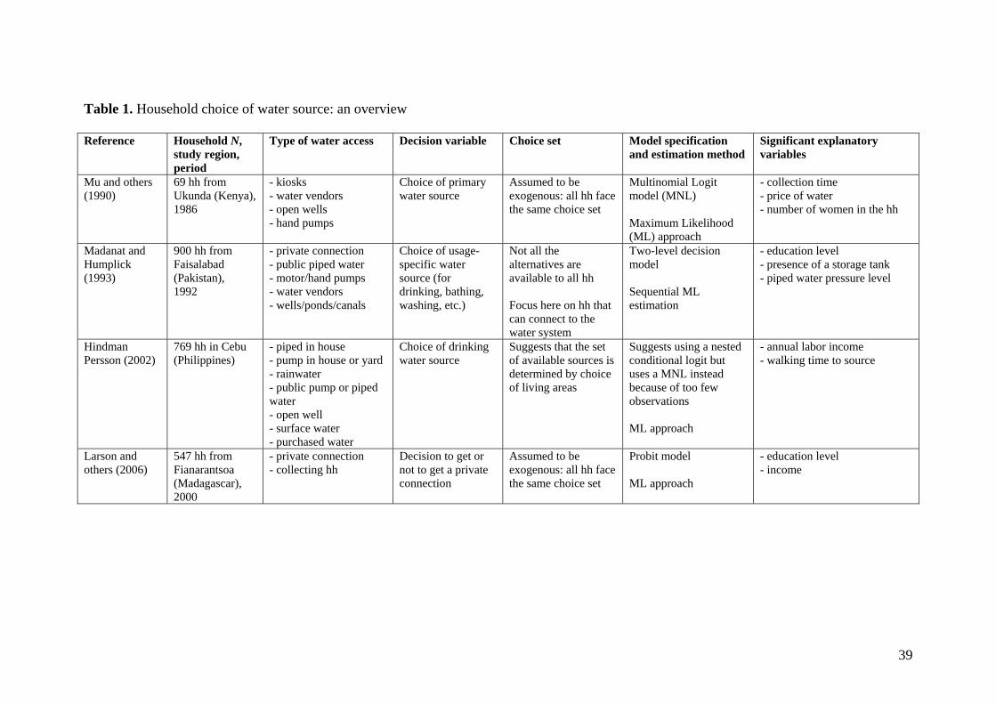
39

Table 1. Household choice of water source: an overview

Reference Household N,

study region, period

Type of water access Decision variable Choice set Model specification and estimation method

Significant explanatory variables

Mu and others (1990)

69 hh from Ukunda (Kenya), 1986

- kiosks - water vendors - open wells - hand pumps

Choice of primary water source

Assumed to be exogenous: all hh face the same choice set

Multinomial Logit model (MNL) Maximum Likelihood (ML) approach

- collection time - price of water - number of women in the hh

Madanat and Humplick (1993)

900 hh from Faisalabad (Pakistan), 1992

- private connection - public piped water - motor/hand pumps - water vendors - wells/ponds/canals

Choice of usage-specific water source (for drinking, bathing, washing, etc.)

Not all the alternatives are available to all hh Focus here on hh that can connect to the water system

Two-level decision model Sequential ML estimation

- education level - presence of a storage tank - piped water pressure level

Hindman Persson (2002)

769 hh in Cebu (Philippines)

- piped in house - pump in house or yard - rainwater - public pump or piped water - open well - surface water - purchased water

Choice of drinking water source

Suggests that the set of available sources is determined by choice of living areas

Suggests using a nested conditional logit but uses a MNL instead because of too few observations ML approach

- annual labor income - walking time to source

Larson and others (2006)

547 hh from Fianarantsoa (Madagascar), 2000

- private connection - collecting hh

Decision to get or not to get a private connection

Assumed to be exogenous: all hh face the same choice set

Probit model ML approach

- education level - income

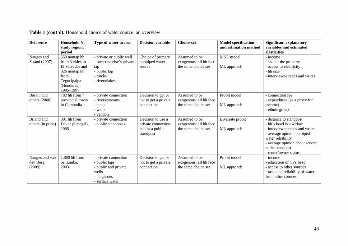
Table 1 (cont’d). Household choice of water source: an overview Reference Household N,

study region, period

Type of water access Decision variable Choice set Model specification and estimation method

Significant explanatory variables and estimated elasticities

Nauges and Strand (2007)

553 nontap hh from 3 cities in El Salvador and 826 nontap hh from Tegucigalpa (Honduras), 1995–1997

- private or public well - someone else’s private tap - public tap - trucks - rivers/lakes

Choice of primary nonpiped water source

Assumed to be exogenous: all hh face the same choice set

MNL model ML approach

- income - size of the property - access to electricity - hh size - interviewee reads and writes

Basani and others (2008)

782 hh from 7 provincial towns in Cambodia

- private connection - rivers/streams - tanks - wells - vendors

Decision to get or not to get a private connection

Assumed to be exogenous: all hh face the same choice set

Probit model ML approach

- connection fee - expenditure (as a proxy for income) - ethnic group

Briand and others (in press)

301 hh from Dakar (Senegal), 2005

- private connection - public standposts

Decision to use a private connection and/or a public standpost

Assumed to be exogenous: all hh face the same choice set

Bivariate probit ML approach

- distance to standpost - hh’s head is a widow - interviewee reads and writes - average opinion on piped water reliability - average opinion about service at the standpost - renter/owner status

Nauges and van den Berg (2009)

1,800 hh from Sri Lanka, 2003

- private connection - public taps - public and private wells - neighbors - surface water

Decision to get or not to get a private connection

Assumed to be exogenous: all hh face the same choice set

Probit model ML approach

- income - education of hh’s head - access to other sources - taste and reliability of water from other sources

40

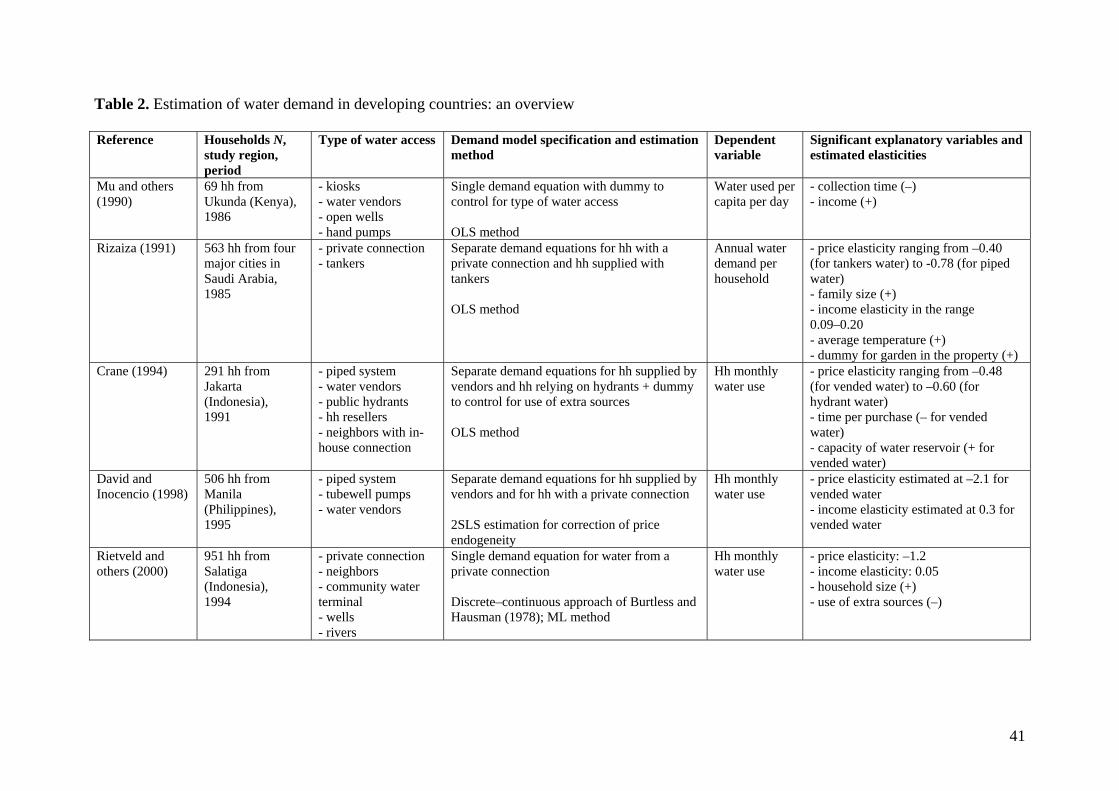
Table 2. Estimation of water demand in developing countries: an overview Reference Households N,

study region, period

Type of water access Demand model specification and estimation method

Dependent variable

Significant explanatory variables and estimated elasticities

Mu and others (1990)

69 hh from Ukunda (Kenya), 1986

- kiosks - water vendors - open wells - hand pumps

Single demand equation with dummy to control for type of water access OLS method

Water used per capita per day

- collection time (–) - income (+)

Rizaiza (1991) 563 hh from four major cities in Saudi Arabia, 1985

- private connection - tankers

Separate demand equations for hh with a private connection and hh supplied with tankers OLS method

Annual water demand per household

- price elasticity ranging from –0.40 (for tankers water) to -0.78 (for piped water) - family size (+) - income elasticity in the range 0.09–0.20 - average temperature (+) - dummy for garden in the property (+)

Crane (1994) 291 hh from Jakarta (Indonesia), 1991

- piped system - water vendors - public hydrants - hh resellers - neighbors with in-house connection

Separate demand equations for hh supplied by vendors and hh relying on hydrants + dummy to control for use of extra sources OLS method

Hh monthly water use

- price elasticity ranging from –0.48 (for vended water) to –0.60 (for hydrant water) - time per purchase (– for vended water) - capacity of water reservoir (+ for vended water)

David and Inocencio (1998)

506 hh from Manila (Philippines), 1995

- piped system - tubewell pumps - water vendors

Separate demand equations for hh supplied by vendors and for hh with a private connection 2SLS estimation for correction of price endogeneity

Hh monthly water use

- price elasticity estimated at –2.1 for vended water - income elasticity estimated at 0.3 for vended water

Rietveld and others (2000)

951 hh from Salatiga (Indonesia), 1994

- private connection - neighbors - community water terminal - wells - rivers

Single demand equation for water from a private connection Discrete–continuous approach of Burtless and Hausman (1978); ML method

Hh monthly water use

- price elasticity: –1.2 - income elasticity: 0.05 - household size (+) - use of extra sources (–)

41

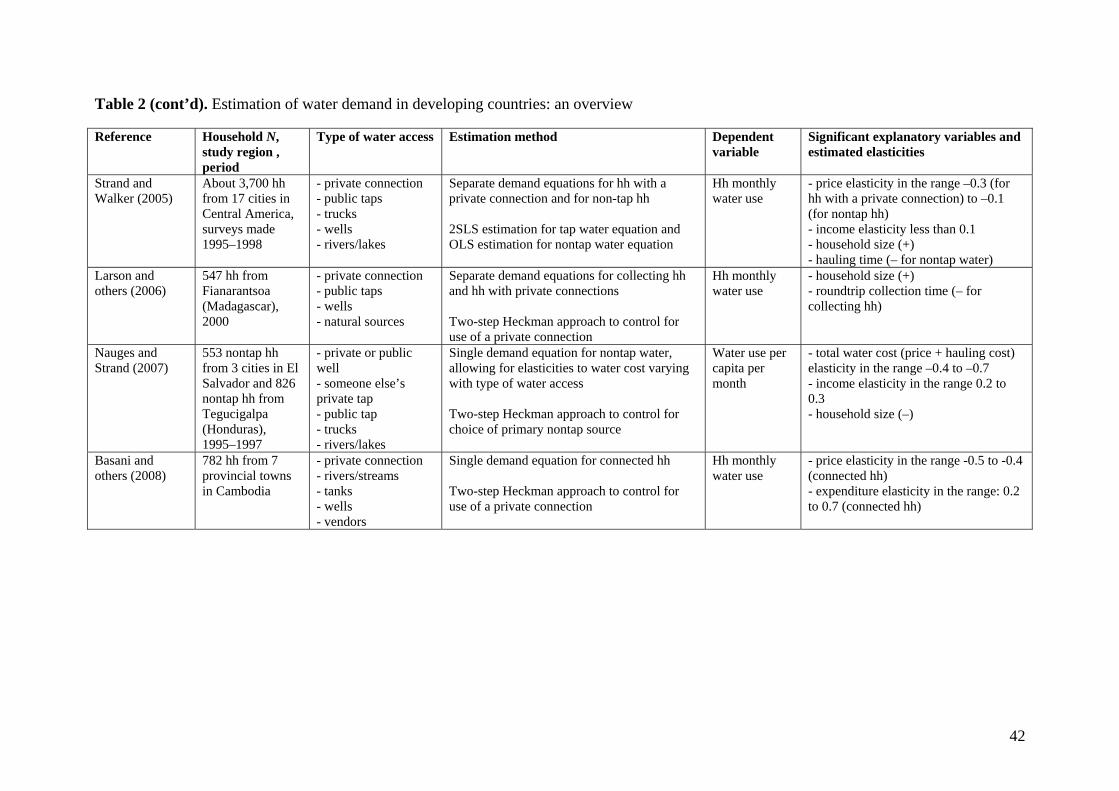
Table 2 (cont’d). Estimation of water demand in developing countries: an overview Reference Household N,

study region , period

Type of water access Estimation method Dependent variable

Significant explanatory variables and estimated elasticities

Strand and Walker (2005)

About 3,700 hh from 17 cities in Central America, surveys made 1995–1998

- private connection - public taps - trucks - wells - rivers/lakes

Separate demand equations for hh with a private connection and for non-tap hh 2SLS estimation for tap water equation and OLS estimation for nontap water equation

Hh monthly water use

- price elasticity in the range –0.3 (for hh with a private connection) to –0.1 (for nontap hh) - income elasticity less than 0.1 - household size (+) - hauling time (– for nontap water)

Larson and others (2006)

547 hh from Fianarantsoa (Madagascar), 2000

- private connection - public taps - wells - natural sources

Separate demand equations for collecting hh and hh with private connections Two-step Heckman approach to control for use of a private connection

Hh monthly water use

- household size (+) - roundtrip collection time (– for collecting hh)

Nauges and Strand (2007)

553 nontap hh from 3 cities in El Salvador and 826 nontap hh from Tegucigalpa (Honduras), 1995–1997

- private or public well - someone else’s private tap - public tap - trucks - rivers/lakes

Single demand equation for nontap water, allowing for elasticities to water cost varying with type of water access Two-step Heckman approach to control for choice of primary nontap source

Water use per capita per month

- total water cost (price + hauling cost) elasticity in the range –0.4 to –0.7 - income elasticity in the range 0.2 to 0.3 - household size (–)

Basani and others (2008)

782 hh from 7 provincial towns in Cambodia

- private connection - rivers/streams - tanks - wells - vendors

Single demand equation for connected hh Two-step Heckman approach to control for use of a private connection

Hh monthly water use

- price elasticity in the range -0.5 to -0.4 (connected hh) - expenditure elasticity in the range: 0.2 to 0.7 (connected hh)

42

Table 2 (cont’d). Estimation of water demand in developing countries: an overview Reference Household N,

study region, period

Type of water access Estimation method Dependent variable

Significant explanatory variables and estimated elasticities

Cheesman and others (2008)

166 hh from Buon Ma Thuot (Vietnam), 2006

- private connection - private wells - vendors

Separate estimation for hh using a private connection only (single equation) and hh combining water from a private connection and well water (system) Two-step Heckman approach to control for use of well water

Hh monthly water use

- price elasticity for piped water estimated at -0.06 for hh using a private connection only and at –0.53 for hh using a private connection and well water - income elasticity: 0.14 - household size (+) - use of a storage tank (+)

Nauges and van den Berg (2009)

1,800 hh from Sri Lanka, 2003

- private connection - public taps - public and private wells - neighbors - surface water

Separate systems of demand equations for piped and nonpiped hh Two-step Heckman approach to control for use of a private connection; Tobit model for censored observations

Water use per capita per month (for piped hh) or per day (for nonpiped hh)

- price elasticity in the range –0.15 to –0.37 for piped hh - collection time (– for non-piped water) - income elasticity: 0.14 for piped hh and 0.20 for non-piped hh - use of a storage tank (+) - hours of piped water availability (+ for piped water) - household size (– for non-piped hh )

43