Climatic Variability and Flood Frequency of the Santa Cruz River, Pima County, Arizona

United States Geological SurveyWater-Supply Paper 2379

Prepared in cooperation with Pima County Depart­ ment of Transportation and Flood Control District

AVAILABILITY OF BOOKS AND MAPS OF THE U.S. GEOLOGICAL SURVEY

Instructions on ordering publications of the U.S. Geological Survey, along with the last offerings, are given in the current-year issues of the monthly catalog "New Publications of the U.S. Geological Survey." Prices of available U.S. Geological Survey publications released prior to the current year are listed in the most recent annual "Price and Availability List" Publications that are listed in various U.S. Geological Survey catalogs (see back inside cover) but not listed in the most recent annual "Price and Availability List" are no longer available.

Prices of reports released to the open files are given in the listing "U.S. Geological Survey Open-File Reports," updated monthly, which is for sale in microfiche from U.S. Geological Survey Book and Open-File Report Sales, Box 25425, Denver, CO 80225.

Order U.S. Geological Survey publications by mail or over the counter from the offices given below.

BY MAIL

BooksProfessional Papers, Bulletins, Water-Supply Papers,

Techniques of Water-Resources Investigations, Circulars, pub­ lications of general interest (such as leaflets, pamphlets, book­ lets), single copies of periodicals (Earthquakes & Volcanoes, Preliminary Determination of Epicenters), and some miscella­ neous reports, including some of the foregoing series that have gone out of print at the Superintendent of Documents, are obtainable by mail from

U.S. Geological Survey, Book and Open-File Report SalesBox 25425

Denver, CO 80225

Subscriptions to periodicals (Earthquakes & Volcanoes and Preliminary Determination of Epicenters) can be obtained ONLY from

Superintendent of DocumentsU.S. Government Printing Office

Washington, DC 20402

(Check or money order must be payable to Superintendent of Documents.)

MapsFor maps , address mail orders to

U.S. Geological Survey, Map SalesBox 25286

Denver, CO 80225

Residents of Alaska may order maps from

ILS. Geological Survey, Map Sales101 Twelfth Ave. - Box 12

Fairbanks, AK 99701

OVER THE COUNTER

Books

Books of the U.S. Geological Survey are available over the counter at the following U.S. Geological Survey offices, all of which are authorized agents of the Superintendent of Doc­ uments.

- ANCHORAGE, Alaska-4230 University Dr., Rm. 101

- ANCHORAGE, Alaska-605 West 4th Ave., Rm G-84

- DENVER, Colorado-Federal Bldg.. Rm. 169,1961 Stout St.

- LAKEWOOD, Colorado- Federal Center, Bldg. 810

- MENLO PARK, California-Bldg. 3. Rm. 3128,345 Mid- dlefieldRd.

- RESTON, Virginia-National Center, Rm. 1C402,12201 Sunrise Valley Dr.

- SALT LAKE CITY, Utah-Federal Bldg., Rm. 8105,125 South State St.

- SAN FRANCISCO, California-Customhouse, Rm. 504, 555 Battery St.

- SPOKANE, Washington-U.S. Courthouse, Rm. 678, West 920 Riverside Ave.

- WASHINGTON, D.C.--U.S. Department of the Interior Bldg., Rm. 2650,1849 C St., NW.

MapsMaps may be purchased over the counter at the U.S.

Geological Survey offices where books are sold (all addresses in above list) and at the following Geological Survey offices:

ROLLA, Missouri- 1400 Independence Rd.

FAIRBANKS, Alaska-New Federal Building, 101 Twelfth Ave.

Climatic Variability and Flood Frequency of the Santa Cruz River, Pima County, Arizona

By ROBERT H. WEBB and JULIO L. BETANCOURT

Prepared in cooperation with Pima County Department of Transportation and Flood Control District

U.S. GEOLOGICAL SURVEY WATER-SUPPLY PAPER 2379

U.S. DEPARTMENT OF THE INTERIOR

MANUEL LUJAN, JR., Secretary

U.S. GEOLOGICAL SURVEY

Dallas L. Peck, Director

Any use of trade, product, or firm namesin this publication is for descriptive purposes onlyand does not imply endorsement by the U.S. Government

UNITED STATES GOVERNMENT PRINTING OFFICE, WASHINGTON : 1992

For sale byBook and Open-File Report SalesU.S. Geological SurveyBox 25425 Denver, CO 80225

Library of Congress Cataloging-in-Publication Data

Webb, Robert H.Climatic variability and flood frequency of the Santa Cruz River, Pima County,

Arizona / by Robert H. Webb and Julio L. Betancourt.p. cm. (Water-supply paper; 2379)

Supt. of Docs, no.: 119.13:2379 Includes bibliographical references. 1. Floods Santa Cruz River Valley (Ariz. and Mexico) 2. Floods Arizona.

3. Hydrometeorology Santa Cruz River Valley (Ariz. and Mexico)4. Hydrometeorology Arizona. I. Betancourt, Julio L. II. Title. III. Series: Geological Survey water-supply paper; 2379GB1399.4.S26W43 1992 92-6507 551.48'9'0979177 dc20 CIP

CONTENTS

Abstract 1 Introduction 1

Purpose and scope 3Acknowledgments 4Hydrologic setting 4

Hydroclimatology of southern Arizona 6Frontal and cutoff low-pressure systems 7Dissipating tropical cyclones 7Monsoonal storms 7

Climatic variability in the 20th century 10Teleconnections and 20th-century variability in global climate 11Frequency of El Nino-Southern Oscillation conditions in the 20th century 11Changes in circulation of the upper atmosphere 15El Nino-Southern Oscillation and precipitation in southern Arizona 17Hydrologic variability in the Santa Cruz River basin 17

Frequency analysis of annual floods in the Santa Cruz River 20Previous estimates of the 100-year flood 20Effects of land use and channel change 23Seasonality of annual floods 23Estimates of 100-year discharges using method of moments, 1970-85 25Trend analysis of the annual flood series 25Flood frequency during El Nino-Southern Oscillation conditions 26

Hydroclimatic flood-frequency analysis of the Santa Cruz River 27Separation of floods by storm types 28Methods of flood-frequency analysis 29Frequency of floods caused by different storm types 32

Summary and conclusions 35 References cited 37

FIGURES

1. Map showing location of study area 22. Graph showing annual flood series for the Santa Cruz River at Tucson,.

Arizona 33. Graph showing average monthly streamflow and monthly streamflow

variability, Santa Cruz River at Tucson, Arizona 64. Maps showing meteorological conditions on days during which three

example floods occurred on the Santa Cruz River at Tucson, Arizona 85. Drawing showing schematic definitions of general circulation flow

types 10 6-22. Graphs showing:

6. Seasonality of cutoff low-pressure systems over the Western United States and generation of tropical cyclones in the tropical eastern North Pacific Ocean 10

7. Variation in the number of tropical cyclones generated in the eastern North Pacific Ocean 11

8. Difference in monthly sea-level pressure between Darwin, Australia, and Tahiti 13

9. Index of Line Island precipitation 1410. Time series of meridional and zonal flow in upper atmosphere from

1899 to 1970 1611. Annual frequency of cutoff low-pressure systems 18

Contents III

12. Correlations between the index of Line Island precipitation for the equatorial Pacific Ocean and precipitation in the Western United States 19

13. Seasonal cumulative departures from mean discharge, Santa Cruz River at Tucson, Arizona 21

14. Duration analyses of daily discharge for two periods, Santa Cruz River at Tucson, Arizona 22

15. Annual flood series for six gaging stations, Santa Cruz River, southern Arizona 24

16. Chronology of 100-year flood estimates for the Santa Cruz River at Tucson, Arizona, 1970-86 25

17. Chronology of moments of the log-transformed annual flood series of the Santa Cruz River at Tucson, Arizona, 1970-86 26

18. Comparison of flood frequency for years with and without El Nifio- Southern Oscillation conditions, Santa Cruz River at Tucson, Arizona 28

19. Largest annual floods at or above base discharge on the Santa Cruz River at Tucson caused by frontal systems, monsoonal storms, and dissipating tropical cyclones 30

20. Mixed-population analysis of floods caused by different storm types between 1915 and 1986, Santa Cruz River at Tucson, Arizona 33

21. Mixed-population analysis of floods caused by different storm types between 1960 and 1986, Santa Cruz River at Tucson, Arizona 34

22. Mixed-population analysis of floods caused by different storm types between 1930 and 1959, Santa Cruz River at Tucson, Arizona 36

TABLES

1. Annual flood series, Santa Cruz River at Tucson, Arizona 42. Estimates of the 100-year flood on the Santa Cruz River at Tucson, Arizona,

made by previous investigators after 1970 53. Annual flood series, Santa Cruz River at Cortaro, Arizona 64. Approximate periods of El Nino-Southern Oscillation conditions in equatorial

Pacific Ocean 155. Matrix of correlation coefficients between Line Island monthly precipitation

and Tucson monthly precipitation, 1900-82 206. Statistical properties and trend-analysis results for five periods of the annual

flood series, Santa Cruz River at Tucson, Arizona 277. Estimates of the 100-year flood for the Santa Cruz River calculated using

different methods and based on different assumptions 298. Floods above base discharge, by storm type, Santa Cruz River at Tucson,

Arizona 319. Floods above base discharge, by storm type, Santa Cruz River at Cortaro,

Arizona 3210. Statistics for annual series of floods caused by three storm types for the Santa

Cruz River at Tucson and Cortaro, Arizona 35

IV Contents

METRIC CONVERSION FACTORS

Multiply inch pound unit By To obtain metric units

millimeter (mm)meter (m)

kilometer (km)square kilometer (km2)

cubic meter per second (m3/s)degree Celsius (°C)

0.039373.28180.62140.3861

35.31°F=1.8(°C)+32

inchfootmilesquare milecubic foot per seconddegree Fahrenheit (F°)

SEA LEVEL

In this report, "sea level" refers to the National Geodetic Vertical Datum of 1929 (NGVD of 1929) a geodetic datum derived from a general adjustment of the first- order level net of both the United States and Canada, formerly called "Sea Level Datum of 1929."

Contents

Climatic Variability and Flood Frequency of the Santa Cruz River, Pima County, Arizona

By Robert H. Webb anc/Julio L. Betancourt

Abstract

Past estimates of the 100-year flood for the Santa Cruz River at Tucson, Arizona, range from 572 to 2,780 cubic meters per second. An apparent increase in flood magnitude during the past two decades raises concern that the annual flood series is nonstationary in time. The apparent increase is accompanied by more annual floods occurring in fall and winter and fewer in summer. This greater mixture of storm types that produce annual flood peaks is caused by a higher frequency of meridional flow in the upper-air circulation and increased variance of ocean-atmosphere conditions in the tropical Pacific Ocean.

Estimation of flood frequency on the Santa Cruz River is complicated because climate affects the magnitude and fre­ quency of storms that cause floods. Mean discharge does not change significantly, but the variance and skew coeffi­ cient of the distribution of annual floods change with time. The 100-year flood during El Nino-Southern Oscillation conditions is 1,300 cubic meters per second, more than double the value for other years. The increase is mostly caused by an increase in recurvature of dissipating tropical cyclones into the Southwestern United States during El Nino-Southern Oscillation conditions. Flood frequency based on hydroclimatology was determined by combining populations of floods caused by monsoonal storms, frontal systems, and dissipating tropical cyclones. For 1930-59, an­ nual flood frequency is dominated by monsoonal floods, and the estimated 100-year flood is 323 cubic meters per second. For 1960-86, annual flood frequency at recurrence intervals of greater than 10 years is dominated by floods caused by dissipating tropical cyclones, and the estimated 100-year flood is 1,660 cubic meters per second. For design purposes, 1,660 cubic meters per second might be an ap­ propriate value for the 100-year flood at Tucson, assuming that climatic conditions during 1960-86 are representative of conditions expected in the immediate future.

INTRODUCTION

Statistical flood-frequency analysis is a commonly used method for assessing flood hazards and risks in the United States (Interagency Advisory Committee on Water Data, 1982; Thomas, 1985). This method uses the annual flood series, which is an array of the largest discharges

that occur each year at a gaging station, to estimate dis­ charges associated with various recurrence intervals, such as 10, 50, and 100 years. Certain recurrence-interval floods, such as the 100-year flood, are then used in engi­ neering design of flood-plain structures or in managing flood plains for development. An example of the use of flood-frequency analysis is the National Flood Insurance Program, which is based primarily on the area of inunda­ tion caused by a 100-year flood (Federal Emergency Man­ agement Agency, 1986).

Flood-frequency analysis requires certain assump­ tions about the statistical properties of the annual flood se­ ries (Interagency Advisory Committee on Water Data, 1982). The annual flood series is assumed to be composed of random events and to be stationary in time; in other words, all floods were randomly generated from a single probability distribution with stable moments, such as the mean and variance. Thus, the floods that compose the an­ nual flood series are assumed to be derived from the same population. Climate is assumed to be invariant, and the ef­ fects of watershed changes on flow conveyance must be negligible (Interagency Advisory Committee on Water Data, 1982). Climatic fluctuations, however, are a source of uncertainty and can lead to misjudgment and misuse of flood-frequency analyses (Dunne and Leopold, 1978, p. 311).

Many of the assumptions required for flood- frequency analysis are not routinely tested and thus could be violated. Obvious hydrologic changes com­ monly result from urbanization and other forms of inten­ sified land use. Influence of climatic variability on flood frequency, however, may be subtle and more difficult to detect. Mixed populations of floods commonly occur, such as those caused by dissipating hurricanes and run­ off from snowmelt. Even where this is demonstrably true, flood-frequency analysis has been used to opera­ tionally estimate flood-recurrence intervals.

The flood record for the Santa Cruz River at Tucson, Arizona (fig. 1), provides one example of an annual flood series (fig. 2; table 1) for which standard flood-frequency analyses yield inconsistent results. Past estimates of the 100-year flood for this river, using slightly different meth­ ods and lengths of record and assuming different statistical

Introduction 1

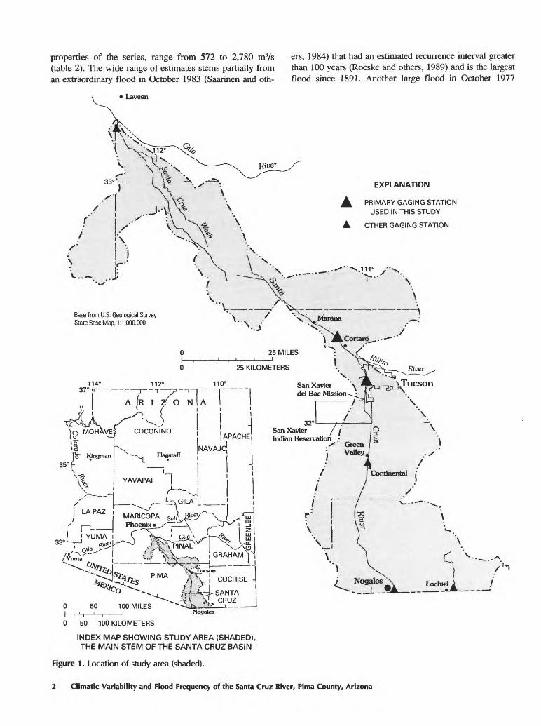
properties of the series, range from 572 to 2,780 m3/s ers, 1984) that had an estimated recurrence interval greater(table 2). The wide range of estimates stems partially from than 100 years (Roeske and others, 1989) and is the largestan extraordinary flood in October 1983 (Saarinen and oth- flood since 1891. Another large flood in October 1977

Laveen

EXPLANATION

A PRIMARY GAGING STATION USED IN THIS STUDY

A OTHER GAGING STATION

\ . -*

Base from U.S. Geological Survey State Base Map, 1:1,000.000

San Xavicr v del Bac Mission

1

i i T -p i-i I

A JR I Z' O N IA I

Lodhuel ) /

Nogales

0 50 100 KILOMETERS

INDEX MAP SHOWING STUDY AREA (SHADED), THE MAIN STEM OF THE SANTA CRUZ BASIN

Figure 1 . Location of study area (shaded).

2 Climatic Variability and Flood Frequency of the Santa Cruz River, Pima County, Arizona

(Aldridge and Eychaner, 1984) had a recurrence interval that, at the time, was estimated to be in excess of 100 years. Overall, six of the seven largest floods in the annual flood series (1915-86) occurred after 1960. After the 1983 flood, alternative methods for estimating design floods, in­ cluding rainfall-runoff modeling, were proposed and used (Michael Zeller, Simons and Li Associates, written com- mun., 1984; Ponce and others, 1985).

The frequent occurrence of large floods in recent years has led several authors to assert that the annual flood series for the Santa Cruz River is nonstationary (Michael Zeller, Simons and Li Associates, written commun., 1984; Hirschboeck, 1985; Baker, 1984; Reich and Davis, 1985, 1986), thus violating the assumption that all floods are de­ rived from the same statistical population. Changes in land use have been blamed for the alleged nonstationarity (Reich, 1984), but larger floods have also occurred in the headwaters of the Santa Cruz River, where land-use changes have been negligible. An alternative explanation is that low-frequency shifts in climate that occur on a time scale of decades have led to a change in the type, inten­ sity, and (or) frequency of storms that cause floods. Changes in flood frequency on the Santa Cruz River coin­ cide with apparent shifts in seasonality and magnitude of floods elsewhere in the Gila River basin.

Purpose and Scope

In 1988, the U.S. Geological Survey in cooperation with Pima County Department of Transportation and Flood Control District undertook a study of changing channel conditions and flood frequency of the Santa Cruz River. Part of this larger study is an assessment of the ap­ plicability of flood-frequency analysis in estimating the re­ currence intervals of floods. Whereas much previous work addressed the influence of channel change on flood fre­ quency, this report uses the hydroclimatic perspective of Hirschboeck (1985, 1987, 1988) to evaluate the link be­ tween low-frequency climatic variability and changes in flood frequency of the Santa Cruz River in Pima County, Arizona.

The hydroclimatology of the Santa Cruz River basin is examined with particular emphasis on storm types that cause floods. The extent of 20th-century cli­ matic variability is analyzed using long-term records of sea-level pressure in the Pacific Ocean, upper atmo­ spheric circulation patterns, and tropical-storm fre­ quency. The time series of these climatic indices are compared with weather records from Tucson and stream- flow records from the gaging station, Santa Cruz River at Tucson, to show the connection between climatic vari-

1600

01200

800

DC<uCOQ 400

I ^ \ '

PERIODS OF FLOODING

I Summer

Fall

Winter

ill.' III mj III

Figure 2. Annual flood series for the Santa Cruz River at Tucson, Arizona. Hydroclimatological year is November 1 to October 31.

Introduction

Table 1. Annual flood series, Santa Cruz River at Tucson, Arizona

[Water year for annual flood series, November 1 to October 31]

Date

12 23-14 1-20-16 -9-08-17 -

8 m i o

8-02-19 -8 no in

8 OI 917 9fi 99

8 17 97

11-17-23 9-18-25 -

9 00 i/^

9-07-27 -

8 ni 989-24-29 g-07-30 -

8 in 71

8 91 11

8-23-34

7 *^£~ 1£.

7-10-37 -

8 ns 78

Discharge, in cubic

meters per second

. _ . 425

142919179

ss

57S4S8

.. __ 96___. _ 323

ss45

_..__.. 295 - 50

761 _. .__ 119_ -._ 173- _-- . 170

799 _ _-- 153 ----- - 93

Discharge, in cubic

meters per Date second

8 14 40 __ g-14-41 8-09-42 0 09 AT,

8 Ifi 44

8-10-45

8-10-47 8-16-48 8-08-49 7 ^n sn8 n9 si8-16-52 7-15-53--

8 rn ss7 99 sfi

8 31 S77 9Q SO

o on so

8-10-60

8 T2 _£ 1

0 OA ff)

227 320 71 47

128 185 306 121 48

109 108 269 142 108 167 271 309 74 86

180 125 174 470 141

Date

8-26-63 ----- n in f.A

7-16-65

8-19-66-

7 1 n /^*ii i m /^*7

8-06-697-20-70 -

8 17 71

10-19-72 3-14-737-08-74 -7 19 7S

9-25-76 m in 778 CO 7R

12-19-78 8 11 on7 97 01

8 97 OO

in n9 0719 98 OA

7-21-86-

Discharge, in cubic

meters per second

1£Q

......... 156__ 166

4Sfi

947 242.._ .. 227_____ 133

54_ 225 . 70 201

671 . 142

709

78

If.

1907

_ _ i 493

987

'Estimated.

ability and hydroclimatology of southern Arizona. Also examined is the influence of climatic variability on the frequency and severity of storm types that cause flood­ ing in southern Arizona. Flood frequency is analyzed using several different methods and assumptions about the data that are based on the hydroclimatic analysis. A mixed-population analysis made on the basis of hydroclimatic segregation of floods and maximum- likelihood analysis is used to estimate flood frequency for floods caused by different storm types in different periods of the 20th century.

Acknowledgments

Ellen Wohl of the Colorado State University, T.W. Swetnam and H.C. Fritts of the University of Arizona, D.R. Cayan of the Scripps Institution of Oceanography, and A.V. Douglas of Creighton University provided some of the climatic data used in this report. Much of this research was inspired by the work of Walter Smith (Smith, 1986) and especially the work of K.K. Hirschboeck (Hirschboeck, 1985, 1987, 1988), both of the University of Arizona. Discussions with Smith and Hirschboeck helped us extend their work in this study.

K.C. Young of the University of Arizona gave access to his collection of National Oceanic and Atmospheric Ad­ ministration Daily Weather Maps, and D.R. Cayan pro­ vided office space and logistical support at Scripps Institution of Oceanography.

Hydrologic Setting

The Santa Cruz River is primarily an ephemeral desert stream and drains 22,200 km2 in southern Arizona and northern Mexico. From its headwaters in the moun­ tains of southern Arizona, the river flows southward into Mexico and loops north to re-enter the United States just east of Nogales. The river flows 105 km from Nogales to Tucson (fig. 1). During major floods, the Santa Cruz River below Tucson flows another 155 km to join the Gila River near Phoenix; however, this reach is typically dry or contains treated sewage or irrigation-return flow. The headwaters of the Santa Cruz are at an altitude of 2,885 m above sea level, the confluence with the Gila River occurs at 310 m, and the average basin altitude above Tucson is 1,234 m above sea level (Roeske, 1978). The basin wide precipitation for the Santa Cruz River basin is 430 mm/yr. Several large historic floods

4 Climatic Variability and Flood Frequency of the Santa Cruz River, Pima County, Arizona

Table 2. Estimates of the 100-year flood on the Santa Cruz River at Tucson, Arizona, made by previous investigators after 1970

[ , no record]

Reference

U.S. Army Corps of Engineers (1972)- Roeske (1978)

Malvick (1980) Federal Emergency Management

Agency (1982) Boughton and Renard (1984) - - -

Michael Zeller (Simons and Li Associates,written commun., 1984)

Eychaner (1984)

Reich (1984)

Ponce and others (1985)

Hirschboeck (1985)

Method or Years of probability record distribution

,\ )

1915 75 (2)1915-75 ( 3)1915-78 (3)

1915-78 (2)1915-79 (4)1915-79 (2)1915-79 (5)

ff>\

1915-81 (2)1915-81 (3)1960-84 (2)1960-84 (7)1962-84 (2)1962-84 ( 7)

8-1/1

848896

1950-80 ( 2)

1 00-year flood,

in cubic meters per

second

1,280575640

1,810

850572666

2,180

1,420626657

1,5302,7301,4202,7801,6601,9001,330

736

'Curve, comparison with floods in other watersheds in southern Arizona.2Log-Pearson type III distribution, method-of-moments fitting.3Log-Pearson type III distribution plus regression analysis.4Log-Pearson type III distribution plus envelope curve.5Log-Boughton distribution, method-of-moments fitting.6Rain, estimated from 100-year rainfall.7Log-Extrerne Value distribution, method-of-moments fitting.8Model, estimated from rainfall-runoff model with 100-year, 24-, 48-, and 96-hour duration storms. This value

is currently being used by Pima County for compliance with Federal Emergency Management Agencyregulations.

on the Santa Cruz River have been described previously (Knapp, 1937; Lewis, 1963; Aldridge, 1970; Aldridge and Eychaner, 1984; Saarinen and others, 1984; Roeske and others, 1989).

Three long-term gaging stations have been main­ tained on the Santa Cruz River in Pima County. The gaging record for the Santa Cruz River at Tucson is the longest but is discontinuous because of a complicated sta­ tion history. Although the first gaging station was installed in 1905 (Schwalen, 1942), the continuous gaging record began in 1915. The station was discontinued in 1981 and was re-established in 1986 (Wilson and Garrett, 1989). In this report, streamflow records for 1915-86 were evalu­ ated, and annual peak discharges were measured or estimated for all years during 1915-86 (fig. 2; table 1). Peaks above a base discharge of 48 m3/s (the partial-dura­ tion series) were measured for 1930-81; however, peaks above base discharge are not known for July and August

1984 or for water year 1985. The mean annual streamflow is 0.64 m3/s at Tucson from a drainage area of 5,755 km2 (Wilson and Garrett, 1989).

The gaging station, Santa Cruz River at Cortaro, Ari­ zona (fig. 1), has a record from 1939-47 and 1950-84, after which the station was discontinued (White and Garrett, 1987). The drainage area above this gaging station is 9,073 km2. Dis­ charges for both the annual flood series (table 3) and the par­ tial-duration series are available for all years of record. The base discharge for the partial-duration series is 76 m3/s. A record from the gaging station, Santa Cruz River at Continen­ tal, Arizona, was not analyzed for flood frequency. Discharges for many floods at this gaging station are inaccurate because flow in an overflow channel around the gaging station was not measured (H.W. Hjalmarson, hydrologist, U.S. Geological Survey, oral commun., 1989).

Averages of monthly discharge for the Santa Cruz River at Tucson indicate that runoff occurs mainly from

Introduction

Table 3. Annual flood series, Santa Cruz River at Cortaro, Arizona

[Water year for annual flood series, November 1 to October 31]

Discharge, in cubic

meters per Date second

8 14 4ft17-11 4n

8 r\f) /I*")

9 24-43 - _ 8-16-44 8 1ft 4S

8 04 46 -

8-15-47 7 ^O SO

7 ?S SI

8-14-52 7 14 S'*

7 74 S4

8-03-55 7 79 56 ___9-01 57 _ -0 ftl S7

8 10 ^s

8-11-60-

8 -T2 sr i

Q 76 f\)

481 221

43 155 160 396 125 212 365 193 172 305 259 470

89 124 124 223 226 181 416 317

Date

8 O/i /^Q

9-10-64 -1 O T> /CC

8-19-66

7 1 "7 /^"7

12-21-67 8-06-697-20-70 -

8 on 71

i n i Q T>

2-22-73 -7 OR 74

9-25-7610-10-77 1 (Y) 78

I * > 10 "70

7-19-80 -9-22-81 -o O1 CO

1ft ft? 87

8 1 /^ Q/1

Discharge, in cubic

meters per second

7ftS4Sft

.. . 475- - _. 169

1 /CO

447oac

-. -_.. 2579SS

104 - _ 331 147

^oo__...__ 651_.._..._ 221

177

TH(\. _ . i 841 ... 145

December through February and July through October (fig. 3). Variability in monthly streamflow is high, and coefficients of variation range from 1 to 6 (fig. 3). Be­ cause the normally defined water year of October 1 to September 30 artificially separates the fall runoff season, a hydroclimatic water year was defined for this report as November 1 to October 31. Redefinition of the water year, which satisfies the assumption of interannual inde­ pendence in annual floods, shifts some floods that occur in October, such as the flood of October 1983, to the previous water year.

Precipitation in southern Arizona has distinct peaks in summer and winter (Sellers and Hill, 1974). Tucson has one of the longest precipitation records (1868-1989) in Arizona, although, like other long-term southwestern stations, it has a complicated station history (Durrenberger and Wood, 1979). The University of Arizona has main­ tained precipitation records since 1891, although the sta­ tion has been moved to five locations within a 15-kilometer radius. There were major station moves in 1894, 1956, 1966, and 1968; the effect of these moves on the statisti­ cal properties of the time series has not been determined. Mean annual precipitation recorded at the University of Arizona in Tucson is 291 mm for the 119-year record. About 129 mm of rain falls between November and June, and 162 mm of rain falls between July and October.

The predominant land use is for livestock grazing, which has occurred for several centuries. Bottomlands are used for agriculture, primarily alfalfa and pecans. Copper is mined in several areas of the drainage basin, mainly near Green Valley, Arizona (fig. 1). Urbanization affects Nogales, Sonora, in Mexico; and Nogales, Green Valley, Tucson, and Marana in Arizona. Green Valley and Tucson incorpo­ rate flood-prone properties along the Santa Cruz River.

HYDROCLIMATOLOGY OF SOUTHERN ARIZONA

Recent hydroclimatological research in southern Ari­ zona links various flood-producing storm types to large- scale atmospheric-oceanic interactions (Hansen and others, 1977; Maddox and others, 1980; Hansen and Schwarz, 1981; Hirschboeck, 1985, 1987; Smith, 1986). Three prin­ cipal types of flood-producing storms and associated upper-atmospheric circulation patterns are described below.

Q 3

2 6

O 4I-

s 2o

1 1 1 1 1 1 1 1 1 i 1 1 1

MONTHLY STREAMFLOW

1 1 1 1 1 1 1 1 1 1 1 _ I

-

ll1 1 1 1 1 1 1 1 1 1

MONTHLY STREAMFLOW VARIABILITY

111 1

WATER YEAR

Figure 3. Average monthly streamflow and monthly stream- flow variability, Santa Cruz River at Tucson, Arizona.

6 Climatic Variability and Flood Frequency of the Santa Cruz River, Pima County, Arizona

Frontal and Cutoff Low-Pressure Systems

Winter storms in southern Arizona originate from large-scale low-pressure frontal systems embedded in the westerly winds from the Pacific Ocean. The storm track moves southward in conjunction with seasonal expansion of a low-pressure cell, called the Aleutian Low, that occurs in the North Pacific. During dry winters, the westerlies fol­ low a path around the north side of a ridge of high pres­ sure off the west coast of North America and into the Pacific Northwest. In wet winters, this ridge is displaced westward, and a low-pressure trough develops over the Western United States. Storms then tend to follow the pre­ vailing winds along the west coast and enter the continent as far south as San Francisco. An example of a frontal system that caused a flood on the Santa Cruz River is the storm of December 17-18, 1978 (fig. 44, fl). The rainfall during this storm ranged from 70 to 250 mm in central Arizona and caused widespread flooding (Aldridge and Hales, 1984).

When a high-pressure ridge in the Pacific is well de­ veloped, low-pressure systems can stagnate and form cut­ off low-pressure systems (fig. 5). The atmospheric conditions that produce cutoff low-pressure systems are discussed in the section titled "Changes in Circulation of the Upper Atmosphere." Cutoff lows that affect Arizona typically form between latitude 30° N. and 45° N. and lon­ gitude 105° W. and 125° W. and have spring and fall maxima (fig. 6). Cutoff lows may intensify off the coast of California before moving inland into Arizona, where they can produce substantial rainfall (Sellers and Hill, 1974; Pyke, 1972; Hansen and Schwarz, 1981). In fall, cutoff low-pressure systems may stall over warm tropical waters and steer dissipating tropical cyclones inland, creating con­ ditions for the idealized probable-maximum precipitation in Arizona (Hansen and Schwarz, 1981).

Dissipating Tropical Cyclones

Occasionally in late summer and early fall, widespread and intense rainfall occurs in southern Arizona because of northeastward penetration of tropical cyclones, which in­ clude hurricanes and tropical storms, from the tropical North Pacific Ocean. An average of 14.1 tropical cyclones are generated each year in the eastern North Pacific Ocean (fig. 7; Rosendal, 1962; Cross, 1988). July and August have the largest number of tropical cyclones 3.4 and 3.5 cyclones per month, respectively (fig. 6). The main area of cyclone generation is off the west coast of Mexico between latitude 10° and 15° N. and between longitude 95° and 100° W.; most tropical cyclones originate more than 300 km south of Cabo San Lucas, the southernmost point in Baja California (Eidemiller, 1978; Cross, 1988).

After leaving their area of origin, most tropical cy­ clones curve west-northwestward and may intensify into

tropical storms or hurricanes. Farther north and west, the storms are dissipated by wind shear and colder water. Some tropical cyclones recurve toward the north and east, steered either by southerly winds ahead of a low-pressure trough, centered over the Pacific Northwest, by a weak trough between two subtropical high-pressure cells, or by circulation associated with a cutoff low-pressure system. These cyclones dissipate over Mexico and the United States, causing intense precipitation and regional flooding (Smith, 1986). Precipitation from dissipating tropical cy­ clones can range from several millimeters to more than 300 mm in 2 to 4 days (Smith, 1986).

Recurving cyclones that have affected southern Ari­ zona were generated most frequently in September and Oc­ tober 72 percent compared with July and August 27 percent (Smith, 1986). Between 1965 and 1984, an average of 1.4 tropical cyclones per year caused precipitation in the Southwestern United States (Smith, 1986). Tropical Storm Octave in late September and early October 1983 is an example of the interaction between a tropical cyclone and a cutoff low-pressure system (fig. 4C) that caused flooding on the Santa Cruz River (Roeske and others, 1989).

The disparity between seasonality of cutoff low- pressure systems and generation of tropical cyclones ex­ plains the greater incidence of recurvature during fall (fig. 6). Although generation of tropical cyclones is at a maxi­ mum in July and August, cutoff low-pressure systems have a maximum incidence in October. The greater incidence of recurvature in fall also is associated with the weakening and southern migration of the Pacific subtropical high and the more frequent appearance of midlatitude troughs at lower latitudes (Eidemiller, 1978). These two phenomena can be­ have synergistically, because dissipating tropical cyclones may contribute moisture to early fall extratropical cyclones from the North Pacific.

Monsoonal Storms

The summer rainy season in Arizona is preceded by strong zonal flow and aridity under direct influence of subsidence from the subtropical high-pressure cell in the eastern Pacific Ocean, which remains displaced to the south during spring and early summer. Near the end of June and early July, the subtropical high-pressure cells shift rapidly northward and induce advection of moist tropical air into Arizona. These synoptic-scale surges (Carleton, 1986) that abruptly break the early summer drought have been likened to monsoonal circu­ lation elsewhere (Tang and Reiter, 1984). The resultant monsoonal storms are characterized by isolated or com­ plex groups of thunderstorms that have a duration of less than several hours (Maddox and others, 1980; Hansen and Schwarz, 1981). Analyses of broad-scale patterns in precipitable water (Reitan, 1960), water-vapor flux

Hydroclimatology of Southern Arizona

140° 135° 130° 125° 120° 115° 110° 105° 100° 95° 90°

30°

SCALE OF NAUTICAL MILESAT VARIOUS LATITUDES

50 100 200 300 iOO 500SURFACE WEATHER MAP AND

STATION WEATHER AT 7:00 A.M. E.S.T.

30°

25°

120° 115° 110° 105° 100° 95° 90° 85°

170° 165° 160° 150° 140°130°120° 100° 80° 70° 60° 50° 40° 35° 30°

B

25

15'

125° 120° 115° 105'

20°

15°

75°

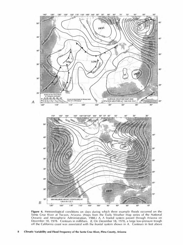
Figure 4. Meteorological conditions on days during which three example floods occurred on the Santa Cruz River at Tucson, Arizona. (Maps from the Daily Weather Map series of the National Oceanic and Atmospheric Administration, 1988.) A, A frontal system passed through Arizona on December 18, 1978. Contours in millibars. B, On December 18, 1978, a large low-pressure trough off the California coast was associated with the frontal system shown in A. Contours in feet above

8 Climatic Variability and Flood Frequency of the Santa Cruz River, Pima County, Arizona

170° 165° 160° 150° 140° 130° 120° 100° 80° 70° 60° 50° 40° 35° 30°

30°

25'

20

15'

125° 120" 115° 110° 105° 100° 90° 85° 80° 75°

170" 165° 160° 150° 140°130°120° 100° 80° 70° 60° 50° 40° 35° 30°

D15° L 500-MILLIBAR HEIGHT CONTOURS AT

7:00 A.M. E.S.T.

25

20°

125° 120° 115° 110° 105° 100'

sea level. C, On October 1, 1983, a cutoff low-pressure system was over the California coast. At the same time, Tropical Storm Octave was off the southwestern tip of Baja California. Contours in feet above sea level. D, On August 23, 1988, generally weak upper atmospheric conditions were associated with monsoonal precipitation in Arizona. Contours in tens of meters above sea level.

Hydroclimatology of Southern Arizona 9

(Rasmusson, 1967), low-level winds (Tang and Reiter, 1984), and regional precipitation (Hales, 1974; Pyke, 1972) suggest that much of the moisture originates from the Pacific Ocean and Gulf of California. Hansen and

Zonal flow

Meridional flow

Cutoff IQW pressure

Figure 5. Schematic definitions of general circulation flow types.

Schwarz (1981) asserted that although the Gulf of Mexico may be the source for much of the day-to-day summer precipitation in the Southwest, it is not the source of moisture for extreme precipitation. Floods caused by monsoonal storms have occurred in almost every year of record for the Santa Cruz River. An ex­ ample of the weak upper-atmospheric circulation of a typical monsoonal storm occurred on August 23, 1988 (fig. 4D). This storm dropped about 70 mm of rainfall in 1 hour in parts of southwestern Tucson.

CLIMATIC VARIABILITY IN THE 20TH CENTURY

Large-scale climatic phenomena affect the hydrocli- matology of southern Arizona and the watershed of the Santa Cruz River. Location of the watershed in a climatic transition zone between temperate and tropical latitudes contributes to distinct seasonal precipitation and streamflow. Streamflow may be a less ambiguous measure of climatic variability than precipitation because it inte­ grates weather phenomena over space and time. In large watersheds such as the Santa Cruz River basin, floods of­ ten occur under a special set of climatic conditions that combine general circulation over North America and sea- surface temperatures in the Pacific Ocean (Hansen and others, 1977). Thus, floods can integrate climatic informa­ tion that might be difficult to detect in more direct mea­ surements of the climate system.

«f

in

0

u. 3LL.Ot-

=>ODCOinLU 9 Z0

ooLL0

£5 1CO

=>z

I I I I I 1 1 1 1 1 1 1 1

[] TROPICAL CYCLONES

| CUTOFF LOWS

-

-

-

_

1 1 1 1 1z CD cc of >:< LU < D_ <

-> "- 5 < s

1 1 1

-

1

-

1

1 0,

_

1-1 1^ >\ (3 H H > 6z ^ -) Q- O O w^ ^ < J" 0 Z D

Figure 6. Seasonality of cutoff low-pressure systems over the Western United States (lat 20° to 45° N., long 100° to 140° W.) and generation of tropical cyclones in the tropi­ cal eastern North Pacific Ocean (lat 5° to 20° N., long 85° to 120° W.).

10 Climatic Variability and Flood Frequency of the Santa Cruz River, Pima County, Arizona

Teleconnections and 20th-century Variability in Global Climate

Precipitation patterns in certain parts of the world are teleconnected, or related over long distances (Ropelewski and Halpert, 1986). For example, the South­ western United States occasionally has abundant precipi­ tation while the Northwestern United States undergoes drought (Lins, 1985). Similarly, the Southeastern United States and much of northern South America are nega­ tively teleconnected. Propagation of teleconnections world­ wide suggests that the same climatic process may control concurrent flooding in Arizona and Florida or in India and Australia.

Teleconnections provide a network for studying the worldwide propagation of low-frequency climatic fluc­ tuations. Using precipitation as an example, summer rainfall in the positively teleconnected areas of India (Mooley and Parthasarathy, 1984), west Africa (Ojo, 1987), and the Sahel (Folland and others, 1986) was above normal for 1930-60 and below normal before and after 1930-60. Changes in ocean temperatures appear to precede the changes in precipitation. In the Atlantic

Ocean, warming occurred in the Southern Hemisphere and cooling occurred in the Northern Hemisphere before about 1925 and after the late 1950's to early 1960's (Folland and others, 1986; Cayan, 1986). The Pacific Ocean also cooled after the early 1960's. This cooling coincided with anomalous upper-atmospheric pressure patterns in the central North Pacific Ocean and south­ ward displacement of the winter storm tracks across western North America (Douglas and others, 1982; Ball­ ing and Lawson, 1982). Cumulative departures from mean temperatures for the United States (Diaz and Quayle, 1980) show significant breakpoints about 1921, 1930, 1952, and 1960. These studies suggest that the middle third of this century (about 1930-60) appears to be climatically distinct from periods before 1930 or after 1960.

Frequency of El Nino-Southern Oscillation Conditions in the 20th Century

The El Nino-Southern Oscillation (ENSO) involves the appearance every 3 to 5 years of anomalously warm water (El Nino) in the equatorial eastern and central

25

20

15

ob_iI 10 o

----- - -FULL SATELLITE COVERAGE-

*ir>ir><o<or-r^ooooa>O1CTJCTJO1O1CTJO1O1O1CTJ

Figure 7. Variation in the number of tropical cyclones generated in eastern North Pacific Ocean between lat 5° N. and 20° N. and long 85° W. and 120° W. Tropical cyclones include hurricanes and tropical storms. Full detection began after 1965 with daily satellite coverage (data from Cross, 1988).

Climatic Variability in the 20th Century 11

Pacific (Rasmusson, 1985; Enfield, 1989). During ENSO events, the sea-surface temperature anomalies are accom­ panied by unusually high sea-level pressure near Indone­ sia and unusually low sea-level pressure near the central equatorial Pacific Ocean (Rasmusson, 1984). The term "La Nina" refers to anomalous cooling in the equatorial Pacific (Bradley and others, 1987). ENSO affects various meteorological and oceanographic conditions worldwide. Teleconnections are particularly pronounced during ENSO conditions (Horel and Wallace, 1981; Elliott and Angell, 1988).

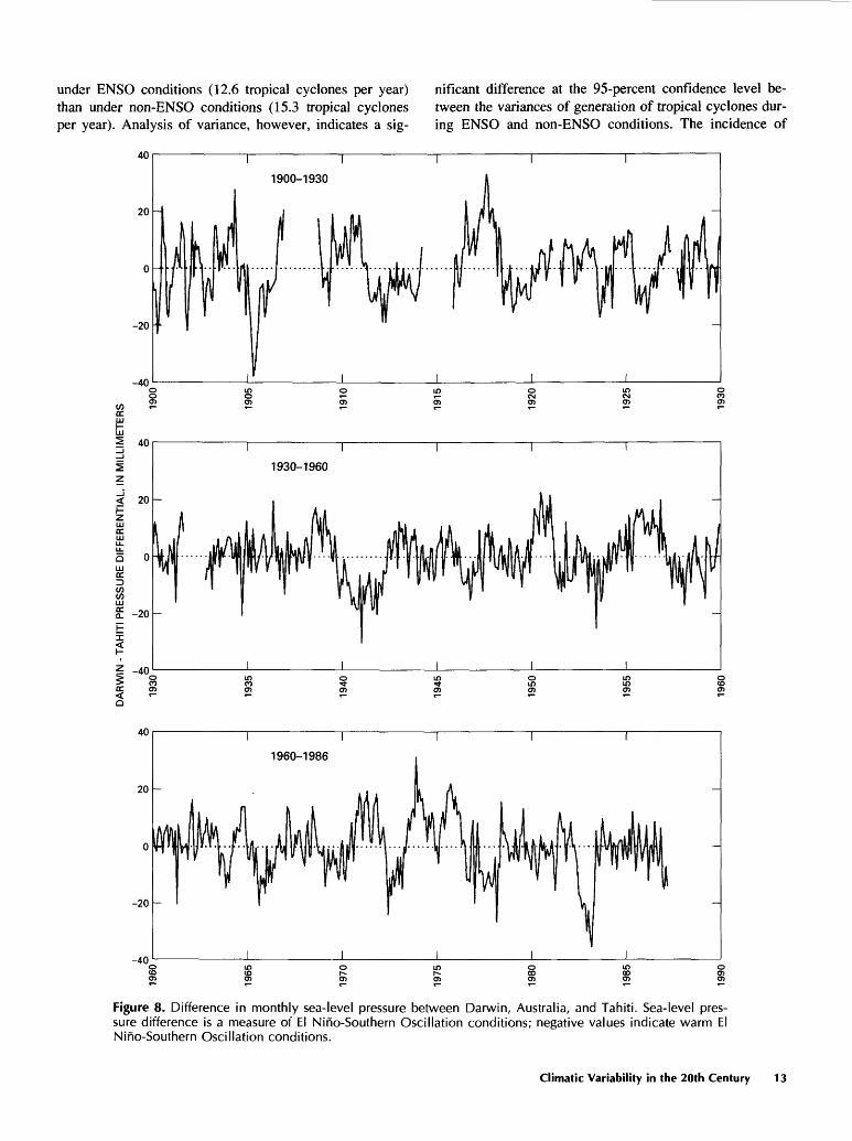
Several indices have been developed that indicate ENSO conditions. The difference in sea-level pressure be­ tween Darwin, Australia, and Tahiti (fig. 8) is commonly used to create an index of the Southern Oscillation. The pressure difference has a significant month-to-month per­ sistence, as indicated by serial autocorrelation coefficients that are significantly different from zero for 8 months. Sev­ eral variations of this index have been developed (Troup, 1965; Wright, 1984; Ropelewski and Jones, 1987). The most common, the Southern-Oscillation Index (SOI), is the pres­ sure difference between Darwin and Tahiti normalized to a mean of zero and a variance of one (Ropelewski and Jones, 1987). Negative values of the Darwin-Tahiti pressure dif­ ference indicate ENSO conditions.

Precipitation in the Line Islands of the equatorial Pa­ cific Ocean (lat 0° to 10° N., long 160° W.) also has been used as an index of ENSO conditions. Distinct precipita­ tion surges occur in these normally dry islands under ENSO conditions (Wright, 1984; Douglas and Englehart, 1984). Positive values of the index of Line Island precipi­ tation (fig. 9) indicate ENSO conditions. This index is sig­ nificantly autocorrelated for 7 months, similar to the Darwin-Tahiti pressure difference. Fewer surges of pre­ cipitation occurred in the Line Islands during 1930-63 (Reiter, 1983).

One of the problems in analyses of ENSO-related phenomena is the use of different criteria for identifying ENSO conditions, such as sea-surface temperatures in Peru, several versions of the SOI, or Line Island precipita­ tion. When there is a high negative correlation between sea-surface temperature in the eastern Pacific Ocean and the SOI, strong ENSO years are easily defined. Differ­ ences arise when defining weaker ENSO years because warming occurs without a large reversal in sea-surface pressure. The Darwin-Tahiti pressure difference and the Line Island precipitation index were used to develop a chronology of 20th-century ENSO conditions (table 4). The chronology differs only slightly from existing chro­ nologies of ENSO (table 4), does not have a denotation of strength, and gives the approximate beginning and ending times for ENSO conditions.

Using the classification in table 4, ENSO conditions recurred on the average of every 3.8 years for 1900-29, every 4.3 years for 1930-59, and every 3.8 years for

1960-86. The seasonality during which ENSO conditions are present has changed during the 20th century. For 1930-60, ENSO conditions often began in the early part of the year and ended in the late part of the year, and the interval between ENSO conditions was as long as 7 years (table 4). Between 1960 and 1986, ENSO conditions typi­ cally began in the middle of the year and lasted until the early or middle part of the following year, and the longest interval between ENSO conditions was 5 years (table 4).

Changes in the statistical properties of the Darwin- Tahiti pressure difference (fig. 8) reflect decadal changes in ENSO conditions. The mean pressure difference is 0.3 millibar (mbar) for 1930-59 and -0.2 mbar for 1960-86. Although the means are not significantly different, the inter-monthly variance in sea-level pressure increased from 43 mbar during 1930-59 to 60 mbar after 1960. The in­ crease in variance after 1960 is statistically significant at a 95-percent confidence level using the nonparametric Squared Ranks Test (Conover, 1971, p. 239-241). Elliott and Angell (1988) also found reduced variances in sea- level pressure at Darwin and Tahiti for about 1920-50. The increased frequency of ENSO conditions suggests an increased occurrence of high sea-surface temperatures, which may affect the occurrence and (or) intensity of fron­ tal storms in the extratropical latitudes.

Precipitation in the Line Islands shows seasonal changes after 1960. Average precipitation from August through February increased after 1960. For September through December, the increases ranged from 12 to 23 percent. The mean for 1960-82 is only 6 percent greater than the record mean; however, the mean for 1976-82 of 127 percent of normal precipitation illustrates the persis­ tent ENSO conditions during this period. This scenario is consistent with the virtual absence, without precedent in the 20th century, of La Nina conditions during 1975-87 (Bradley and others, 1987).

ENSO conditions affect the hydroclimatology of the southwestern United States, particularly Arizona (Andrade and Sellers, 1988; Douglas and Engelhart, 1984). Areas teleconnected with the equatorial Pacific Ocean, such as the Southwestern United States, have increased variability of precipitation (Nicholls, 1988). Winter frontal storms are more numerous and intense during certain ENSO years (Rasmusson, 1984, 1985) because of an intensified Aleutian low (Yarnal and Diaz, 1986). The probabilities for genera­ tion and recurvature of tropical cyclones change during ENSO conditions, but the advection of moisture needed to fuel monsoonal storms is reduced (Reyes and Cadet, 1988). Hypothetically, ENSO conditions could reduce the number of monsoonal storms but increase the number of frontal systems and tropical cyclones that affect Arizona.

ENSO affects the variability of tropical-cyclone gen­ eration. After 1965, all tropical cyclones generated in the eastern North Pacific Ocean were detected by weather sat­ ellites. On average, fewer tropical cyclones were generated

12 Climatic Variability and Flood Frequency of the Santa Cruz River, Pima County, Arizona

under ENSO conditions (12.6 tropical cyclones per year) than under non-ENSO conditions (15.3 tropical cyclones per year). Analysis of variance, however, indicates a sig­

nificant difference at the 95-percent confidence level be­ tween the variances of generation of tropical cyclones dur­ ing ENSO and non-ENSO conditions. The incidence of

40

20

-20

-40

1900-1930

I 40

< 20 -

-40

Figure 8. Difference in monthly sea-level pressure between Darwin, Australia, and Tahiti. Sea-level pres­ sure difference is a measure of El Nino-Southern Oscillation conditions; negative values indicate warm El Niho-Southern Oscillation conditions.

Climatic Variability in the 20th Century 13

tropical cyclones dissipating over Arizona increases during ENSO conditions. The largest numbers of dissipating tropi­ cal storms per year that affected the Southwestern United

States occurred in the ENSO years of 1925-26, 1939, 1957-58, 1976-77, and 1982-83 (Smith, 1986). In Septem­ ber, the peak month for recurvature, 3.4 tropical cyclones

300

250 -

200 -

150 r

100 -

Figure 9. Index of Line Island precipitation (Wright, 1984), representing percent-of-normal precipitation for several stations. Sustained periods with values greater than 100 indicate El Nino-Southern Oscillation conditions.

14 Climatic Variability and Flood Frequency of the Santa Cruz River, Pima County, Arizona

Table 4. Approximate periods of El Nino-Southern Oscillation conditions in equatorial Pacific Ocean

[Note tendency for El Nino-Southern Oscillation conditions to begin in the early part of the calendar year between 1930 and 1960, compared to midyear before 1930 and after 1960]

El Nino-Southern Oscillation conditions agree with

Period of time

From

Late 1899 Mid- 1902

Early 1905 Mid-1911 Mid-1914 Mid-1918 Mid- 1923 Mid- 1925

Mid- 1930 Early 1932 Mid- 1939

Early 1946 Early 1951 Early 1953 Early 1957

Mid- 1963 Early 1965 Early 1969 Mid- 1972 Mid- 1976 Mid- 1982 Mid- 1986

To

Mid- 1900Early 1903 Mid- 1906Mid- 1912Mid-1915 -T atf* 1010

T at*> 1 GO 3

Mid- 1926

Early 1931 -T ata 10^9

Early 1942Late 1946 -T ate 10S1

T at*> 1 CK3

Mid- 1958

Mid- 1966 -T atf IQfiQ

Early 1973Early 1978Mid- 1983

Early 1987

Southern Oscillation

Index

. ___ YesVac

Vac

Vac

Vac

. ___ YesVe-c

Vat.

.... NoVac

___ Yes___ Yes___ Yes

Vac

Vac

Vac

Vac

___ Yes___ Yes

. ___ Yes

___ Yes

Line Island Precipitation

Index

Yes Yes Yes Yes Yes Yes Yes Yes

Yes Yes Yes Yes Yes Yes Yes

Yes Yes Yes Yes Yes Yes

Quinn and others

(1987)

Yes Yes Yes Yes Yes Yes Yes Yes

Yes Yes Yes No Yes Yes Yes

No Yes No Yes Yes Yes Yes

Rasmusson (1984)

Yes Yes Yes Yes Yes Yes Yes Yes

Yes Yes Yes Yes Yes Yes Yes

Yes Yes Yes Yes Yes Yes

per year were generated during ENSO years compared with 2.3 tropical cyclones per year during non-ENSO years. The annual number of tropical cyclones generated increased from 13.7 for 1965-70 to 16.4 for 1983-88 (fig. 7).

The different recurrences of ENSO during different periods of the 20th century possibly stem from trends in upper-atmospheric pressure over the Northern Hemisphere (Reiter, 1983). Namias (1986) observed that periods of high persistence in the westerly winds precede the North­ ern Hemisphere mature stage of ENSO by as much as 1 year, which implies that abnormal atmospheric circulation could induce ENSO conditions. Climatic variability on a decadal scale could be driven by long-term increases in the midtropospheric subtropical westerlies and in the fre­ quency of ENSO conditions (Namias and others, 1988). Changes in general atmospheric circulation, therefore, need to be considered in concert with ENSO conditions for an explanation of decadal-scale variability on hydroclima- tology in Arizona.

Changes in Circulation of the Upper Atmosphere

In the temperate latitudes, the upper atmosphere gen­ erally alternates between two different types of large-scale motion. Zonal flow occurs when winds in the upper atmo­ sphere are predominantly westerly in direction (fig. 5) and usually results in fair weather in Arizona. Meridional flow occurs when winds follow an undulating, wavelike path across the Northern Hemisphere (figs. 4B, 5). Meridional flow creates ridges of high pressure and troughs of low pressure that may be stationary for long periods over North America. Meridional flow allows storms to intensify with tropical moisture and penetrate into the Southwest. The spatial distribution of precipitation in the Western United States depends on the axial position, orientation, amplitude, and wavelength of troughs and ridges (Granger, 1984). Meridional flow may break down in transition to zonal flow, and low-pressure eddies in troughs may be­ come separated from the general circulation and become cutoff low-pressure systems (figs. 4C, 5; Douglas, 1974).

Climatic Variability in the 20th Century 15

The long-term frequency of circulation patterns in the Northern Hemisphere has been addressed by Dzerdzeevskii (1969, 1970), Kalnicky (1974), Barry and others (1981), and Carleton (1987). Zonal flow was more common for 1930-60 than before or after (Dzerdzeevskii, 1969; Kalnicky, 1974; Balling and Lawson, 1982). Dzerdzeevskii (1970) classified Northern Hemisphere circulation for each day for 1899-1969

as zonal, meridional, or transitional (fig. 10). The Dzerdzeevskii circulation types shifted to a greater incidence of zonal flow around 1930 and back to a dominance by meridional flow beginning in the 1950's (fig. 10; Dzerdzeevskii, 1969). The greater incidence of meridional flow in the latter part of the series has continued into the 1980's (Balling and Lawson, 1982).

350

300

250

200

150

100

50

1 ' I ' I

MERIDIONAL CIRCULATION

o 300

250

200

150

100

50

' \ ' \

ZONAL CIRCULATION

Figure 10. Time series of meridional and zonal flow in upper atmosphere from 1899 to 1970 (Dzerdzeevskii, 1970). Dotted lines represent the 6-year running mean.

16 Climatic Variability and Flood Frequency of the Santa Cruz River, Pima County, Arizona

The temporal incidence of cutoff low-pressure sys­ tems suggests another measure of fluctuations in general circulation. As noted previously, cutoff low-pressure systems evolve during the breakdown of meridional flow in the upper atmosphere. Generally, a low-pressure cell is present near latitude 55° N. and longitude 140° W., and low-pressure eddies move eastward from that area to produce precipitation across the United States. During meridional flow, some low-pressure eddies move as far southward as latitude 25° N. become detached from the westerly circulation pattern, and stagnate before slowly drifting eastward.

For 1945-59, the number of cutoff low-pressure sys­ tems that occurred over the continental and southwestern United States averaged 31.9 and 21.3 per year, respec­ tively (fig. 11). For 1960-88, this number decreased to 29.3 per year over the continental United States and 19.2 per year over the Southwest. Concurrently, the variance decreased by about 60 percent in both cases, and the de­ crease is significant at the 95-percent confidence level us­ ing the Squared Ranks Test. These results suggest a greater continuity of meridional flow after 1960.

The incidence of cutoff low-pressure systems in cer­ tain months is significantly correlated with ENSO condi­ tions. For example, the number of cutoff lows over the Southwestern United States is negatively correlated with the sea-level pressure difference in January (r = -0.460), March (r = -0.316), and November (r = -0.474). The av­ erage numbers of cutoff low-pressure systems are similar during ENSO and non-ENSO conditions; however, season­ ally, the average numbers of cutoff lows increases slightly under ENSO conditions for the months of March, October, and November. For example, the average numbers of cut­ off lows during March are 3.15 for ENSO conditions and 2.32 for non-ENSO conditions. The joint occurrence of a slight increase of cutoff low-pressure systems in the fall with a slightly increased generation of tropical cyclones suggests increased incidence of tropical cyclones that dis­ sipate over Arizona during ENSO conditions.

El Nine-Southern Oscillation and Precipitation in Southern Arizona

Climate in southern Arizona is teleconnected with the equatorial Pacific Ocean. For example, correlations be­ tween SOI and seasonal precipitation for many Arizona stations are statistically significant and negative (Andrade and Sellers, 1988; Ropelewski and Halpert, 1986; and Douglas and Englehart, 1984). Andrade and Sellers (1988) found that precipitation in Arizona and western New Mexico is enhanced in the normally dry spring and fall during ENSO conditions. They suggested that warm sea- surface temperatures off the west coasts of Mexico and California (1) provide the necessary energy for the devel­ opment of strong west coast troughs, (2) weaken the

tradewind inversion and thus allow moist air to penetrate into the Southwest, and (3) cause stronger, more numerous Pacific tropical cyclones than usual. Douglas and Englehart (1984) found significant positive correlations be­ tween the index of Line Island summer precipitation and precipitation in the southwestern United States during Oc­ tober, November, and the following February and March (fig. 12). These months are also ones in which the inci­ dence of cutoff low-pressure systems increased under ENSO conditions. Southern Arizona and southern Califor­ nia yield the highest positive correlations for each of these months for latitudes south of 40° N. (fig. 12).

For 1900-82, seasonal teleconnections are reflected in the correlation coefficients between monthly precipita­ tion at the University of Arizona at Tucson station and the index of Line Island precipitation for the current and pre­ vious (lag 1) year. Significant positive correlations were obtained between precipitation in the Line Islands for all months from the previous June to the current April and precipitation at the University of Arizona from February to May (table 5). Significant correlations were also obtained between Line Island precipitation in summer and fall with precipitation at the University of Arizona between October and November (table 5). Some of these correlations imply a 4- to 6-month lag in the midlatitude atmosphere-ocean response to processes that occur at the equator. Significant relations between precipitation in the Line Islands and Tucson for the same month, however, suggest a more di­ rect link to tropical cloud masses moving northeast from the central equatorial Pacific Ocean.

Betancourt (1990) analyzed the effect of ENSO conditions on Tucson precipitation using a 36-month period centered on June of an average year with ENSO conditions. Precipitation is significantly increased in most months during and 1 year after ENSO conditions; precipitation for April through June and October is sig­ nificantly higher than for non-ENSO conditions. Sig­ nificantly reduced precipitation in August, during ENSO conditions, indicates a suppression of summer monsoonal precipitation under ENSO conditions. Sell­ ers (1960) found a negative correlation between Sep­ tember and July and August precipitation for 1898 to 1959 in Arizona. Under ENSO conditions, precipitation begins earlier in fall months in the southwestern United States (Kiladis and Diaz, 1989). Sellers (1960) and Betancourt (1990) suggested that atmospheric condi­ tions that are conducive to monsoonal precipitation are somewhat exclusive of precipitation from dissipating tropical cyclones.

Hydrologic Variability in the Santa Cruz River Basin

Various indices and proxy records indicate shifts in climate around 1930 and 1960. Because Arizona's climate

Climatic Variability in the 20th Century 17

50

40

30

20

10

fe 50

40

30

20

10

I I I

CONTINENTAL UNITED STATES

i i i rSOUTHWESTERN UNITED STATES

Figure 11. Annual frequency of cutoff low-pressure systems, which are defined as 2 days with one closed geopotential height on a 500-millibar height map (National Oceanic and Atmospheric Administration, 1988). Cutoff low-pressure systems occur over the Conti­ nental United States between lat 20° N. and 45° N. and long 65° W. and 140° W. and in the Southwestern United States between lat 20° N. and 45° N. and long 100° W. and 140° W.

18 Climatic Variability and Flood Frequency of the Santa Cruz River, Pima County, Arizona

45

NOVEMBER

AREA WITH CORRELATION COEFFICIENT SIGNIFICANTLY DIFFERENT FROM ZERO

JANUARY

EXPLANATION

MARCH

0 LINE OF EQUAL CORRELATION COEFFICIENT Interval is .15

+.55 EXTREME CORRELATION COEFFICIENT AND VALUE

Figure 12. Correlations between the index of Line Island precipitation for the equatorial Pacific Ocean and precipita­ tion in the Western United States (Douglas and Englehart, 1984).

Climatic Variability in the 20th Century 19

Tabl

e 5.

Ma

trix

of

corr

elat

ion

coef

ficie

nts

betw

een

Line

Isl

and

month

ly p

reci

pita

tion a

nd T

ucso

n m

onth

ly p

reci

pita

tion

, 1900-8

2

[Com

pari

son

begi

ns w

ith L

ine

Isla

nd p

reci

pita

tion

in J

une

of th

e pr

evio

us y

ear t

o ch

eck

for l

ag e

ffec

ts o

n T

ucso

n pr

ecip

itatio

n. P

ears

on c

orre

latio

n co

effi

cien

ts g

reat

er th

an o

r equ

al to

0.2

2 ar

e si

gnif

ican

tly

diff

eren

t fro

m z

ero

at th

e 95

-per

cent

con

fide

nce

leve

l. Si

gnif

ican

t val

ues

are

unde

rsco

red.

Not

e th

at c

orre

latio

n co

effi

cien

ts g

reat

er th

an 0

.28

are

sign

ific

antly

dif

fere

nt fr

om z

ero

at a

99-

perc

ent c

onfi

denc

e le

vel]

o o QL

Inde

x of

Lin

e Is

land

pre

cipi

tatio

n

June

Jan.

Feb.

--

Mar

. -

Apr

. -

May

-

June

-

July

Aug

. -

Sept

. -

Oct

. -

Nov

. -

Dec

. -

5|

"> ir

: ot

> 3

O

[I L C

»

3 Co-,

°o «a n IS :* i so 37

) first

estimated

n*>^

IA

4.

1*

n£ j

ff3

O)

O O 3 I O) 2 SL | o 1 s rT on

3' o 3

t/> r a.

> on 00 g p O) y

--0.

11

- -2

2 -

.25

- .1

4 -

.02

- .0

2 -.

05

- -.

01

- .0

6 .0

0 -.

01

.02

^ (^^

1 O)

Ol p n 2 N H 1 o»

tfl 5

" <

01a^g

. sr

1 ;d

public awareness of

flo

ore the

flood

of

October 0 d-freque

ncy estima

1983,

estimates

of f ?

July

Aug

. Se

ptO

ct.

-0.1

5 -0

.13

0.03

-0

.09

.27

.26

.37

.34

.28

.47

.42

.45_

.16

.27

.21

.26

.11

.17

.14

.16

.12

.12

.19

.14

-.06

-.

15

-.16

-.

17

.00

-.10

-.

15

-.11

-.

13

.08

.12

.14

-.17

.0

3 -.

06

.06

-.20

.2

2 .1

6 .1

7 .0

4 .0

6 -.

06

.10

? CL 8,

i? 0 3* Co 00

U)

0 3 f

01 n N O)

o ffi <8 o' c s Estimates

of

the

1

0( » n JU ^ HI o o Q.

zS _i m

Jo £c ENCY

ANALYS

IS OF

SANT

A CRU

Z RIVER > .NNUA

L FLOO

I

w (/>

hC

O

3

<=

"*

rtO

i-2

3^3

0

S <

3

o o

3 ^ fall

and

winte

r precipi

tati er precipita

tion durin

g pe

f

ENSO

conditions

before H_

3

OSO

§

3

£

S.

Po c

« 5

|2>

~C

L ^

5.

gs 3-

o>

0*9

s ^

* 1

i '

c«

'O

\O

O)

1-1

s^i

?l"

Nov

.

-0.0

8 -4

3.

.47

.20

.22

.06

-.19

-.

15

.05

-.13

.1

3 .0

4

T3 P 2 S 1 S a.

a. 1 o i I ££

C

/3 3 t/> c c« 3 ! f 0) =r b 0)

Co C*J £̂ 0 &> sr 1 § 8,

ft n 1 r" dative-departure cu O)

Dec

. Ja

n.

Feb.

M

ar.

Apr

. M

ay

June

Ju

ly

Aug

. Se

pt.

Oct

. N

ov.

Dec

.

-0.0

2 -0

.01

-0.0

3 0.

07

0.01

-0

.05

0.04

0.

02

-0.1

4 -0

.03

0.02

-0

.06

-0.0

2 .3

3 .3

6 .2

7 .1

9 .2

1 .0

8 .1

2 -.

01

.05

.08

.05

.03

.16

.51

.38

.41

.M

.24

.19

.15

.04

-.07

.0

5 .0

0 .0

1 -.

01

.31

.3.3

.2

5 .2

4 .2

8 .2

1 .2

8 .1

4 .2

6.

.19

.12

-.08

.1

0 .2

5 .1

7 .1

9 .2

2 .2

4 .1

1 .2

3 .0

6 .1

3 .2

9 .2

5.

.18

.23

.09

.05

.06

.07

.00

-.01

.0

6 .0

6 .1

2 .1

1 .1

6 .1

4 .1

4 -.

10

-.10

-.

09

-.14

-.

12

-.26

-.

28

-.17

-.

19

-.10

-.

16

-.19

-.

22

-.14

-.

08

-.10

-.

13

.10

-.15

.0

8 .0

5 -.

07

-.06

.0

5 .0

5 .0

9 .0

4 .0

2 .0

3 .0

5 .1

4 .0

9 .1

2 .2

3 .1

8 .0

1 .0

6 .1

0 .1

6 .0

6 .0

3 .0

4 .1

4 .2

3 .3

0 .2

2 .3

4 .2

1 .2

1 .3

J .2

9 .2

9 .1

9 .1

7 .2

0 .1

7 .1

7 .1

3 .3

3 .2

5 .3J

_ .2

9 .3

4 .2

7 .2

4 .0

8 .0

9 .1

1 .1

5 .1

5 .0

8 .1

6 .1

1 .1

5 .1

9 .2

0 .2

4 .0

7

O) o O) a. v>

O) o *5* >-t 1 0 v> S?

E-5

&S

»

o =

3g

g.^

«a»

go

g5

r9&

^a?3

._c

^ y

^^^

'^i

r^ f^

r-i rt

^ "'I

(^^

^* CTQ

f^

o^D

s^

1 ii

rtO

)^y

^p ^y

^^ r

^ ^

^

ffS

.ill'o

SS

l^s^

slss

afcp

iiIi

^li.i

wiH

iii

iiil

i!|!

i!ii

!l!i

llr^

t!lf

l^t

??§

.=

Ps

a|§

S.i

Ssi.

lsS

-«5

!oi-

sl»

§. §

S-S

>|3

^|iP

||ll

-a=

l|i-

||^|s

s|||

5||||.|

^ttfT

^N

^

!-i

^..

SO

0)

^

3-O

) c«

-3

O)

K

j3

O)

p^ffi^

_,

T

l «5

T ^O

S

O)

3

t^i

C

CTO

^S

M^

1"1

' ^

C

Dh^ph^

^.

.j

>^

^)

i^.

fl)

^.

OO

^

J^

.**

Q

r-f

S^ll

ll'

^^sll

lill

.^?!"

1

1* ? 1

' ? I'

? I

' ? I

1 s,

w s-

a s-

" f«

iJ

3

t*

- 8

§ £

so

O)

£

Z;

^ S

°'

0. with

these

climati

c proce

s and

hydrolo

gic regim

es perio

ds of

the

20th

centur

>-59,

and

1960-86

were

;s, some differenc

e ould

be

expec

ted The

perio

ds of

191

losen for

compari 1

? S

? 3'

years. Schwalen (1942) estimated the 100-year flood to be 450 m3/s from a record length of 27 years. Recent esti­ mates range from 572 to 2,780 m3/s (table 2) and were

derived by applying different methods and assumptions to varying lengths of record both before and after the 1983 flood (table 2).

-20

-40

-60

FALL RUNOFF

S

Figure 13. Seasonal cumulative departures from mean discharge, Santa Cruz River at Tucson, Arizona.

Frequency Analysis of Annual Floods in the Santa Cruz River 21

After the flood of 1983, local authorities reacted to using 100-year-frequency rainfall of 24-hour, 48-hour,discrepancies in the 100-year flood estimates by com- and 96-hour durations was used in one study (Ponce andmissioning studies and amending existing flood-plain others, 1985). The model was calibrated by hindcastinglegislation. A deterministic hydrologic simulation model the runoff hydrograph of the flood of October 1983.

1000 p

100

10

0.1

1000

100

10

0.10.1

JULY-AUGUST

EXPLANATION

1915-1929

1930-1959

______ 1960-1981

SEPTEMBER-OCTOBER

EXPLANATION

1915-1929

1930-1959

______ 1960-1981

1 10

PERCENT OF DAYS EXCEEDED

100

Figure 14. Duration analyses of daily discharge for two periods, Santa Cruz River at Tucson, Arizona.

22 Climatic Variability and Flood Frequency of the Santa Cruz River, Pima County, Arizona

Some of the assumptions relating to tributary inflow dur­ ing the flood of October 1983 have been questioned (Hjalmarson, 1987). On the basis of the rainfall-runoff model, both Pima County and the city of Tucson adopted a "regulatory flood" of 1,700 m3/s and a "design flood" of 1,980 m3/s in 1985 for the reach between the San Xavier del Bac Mission and the confluence with the Rillito River (fig. 1). The regulatory flood is used for compliance with the National Flood Insurance Program, whereas the design flood is used for design of bridges and other flood-plain structures.

Effects of Land Use and Channel Change

Reich (1984), Michael Zeller (Simons Li and Asso­ ciates, written commun., 1984), and Reich and Davis (1985, 1986) attributed the change in flood frequency to increased channelization, improved channel conveyance, and reduced channel storage upstream from Tucson since establishment of the gaging station, Santa Cruz River at Tucson, in 1915. Changes in channel topography, such as those that evolved from arroyo-cutting along the Santa Cruz River (Cooke and Reeves, 1976; Betancourt and Turner, 1988; Betancourt, 1990), are known to alter con­ veyance of flood waves (Burkham, 1981). The result would be an increase in the peak discharge downstream for the same volume of runoff.

The Santa Cruz River did not have an entrenched channel near the south boundary of the San Xavier Indian Reservation (fig. 1) in 1915, when the gaging station was established at Tucson. In the reservation, the channel deep­ ened 3 to 5 m between 1915 and the late 1930's and an­ other 2 to 3 m since then. The channel bottom at Tucson incised 3 to 5 m after 1946 (Aldridge and Eychaner, 1984) apparently because of encroachment of the channel by landfills and highway construction. Hypothetically, the flood in December 1914, which produced a peak discharge of 425 m3/s, would yield a much higher peak if routed through the modern incised channel. Conversely, the peak discharge of 1,490 m3/s in October 1983 might have been much less if it had flowed through the discontinuous ar- royo system that existed in 1915. Preliminary results using a flow-routing model, however, yielded only an approxi­ mate 15- to 20-percent decrease in discharge by routing the flood of 1983 through the 1915 channel (H.W. Hjalmarson, hydrologist, U.S. Geological Survey, oral commun., 1989). Local channel erosion, therefore, is not the sole reason for changes in the annual flood series.

Annual floods have increased in size at all gaging stations on the Santa Cruz River (fig. 15). At Lochiel, a flood in August 1984 was larger than the flood of October 1983 (fig. 15A). No significant change in land use has oc­ curred upstream from the gaging station at Lochiel. At Nogales (fig. 155), where land use in Mexico could have

altered flow conveyance, five of the six largest floods oc­ curred between 1968 and 1983. The annual flood series for other gaging stations on the Santa Cruz River also show an increase in annual peaks (fig. 15C, E, F). At Tucson, six of the seven largest floods occurred after 1960 and five of these occurred in fall or winter (table 1; fig. 15D).

Although land use and changes in channel convey­ ance undoubtedly have increased flood discharges to some unknown extent, climatic effects are the only com­ mon link among the six gaging stations on the Santa Cruz River. Only the very largest floods, as in October 1983, are sustained from the headwaters to the juncture with the Gila River near Laveen. At Lochiel, flows in the Santa Cruz River could not have been affected sig­ nificantly by land use, yet peak discharges have in­ creased since 1960 (fig. 15/4). The August 1984 flood at Lochiel, the peak of record, was larger than the October 1983 flood, which indicates that the apparent changes are not caused by a few isolated large floods. Changes in the hydroclimatology of the basin are reflected by a shift in the seasonality of annual flood peaks, which is also the most striking symptom of the underlying climatic control of flood frequency.

Seasonality of Annual Floods

The annual flood series of the Santa Cruz River at Tucson shows a lack of uniformity in the seasonality of flood peaks (table 1, fig. 2; Keith, 1981; Hirschboeck, 1985; Betancourt and Turner, 1988) that may partly ac­ count for the increase in annual peaks since 1960. Floods in July and August accounted for 75 percent of the annual peaks for 1915-86, and summer had the larg­ est and least-variable monthly discharges (fig. 3). For 1915-29 and 1960-86, however, 53 percent and 39 per­ cent, respectively, of the annual flood peaks occurred in fall (September to October) or winter (November to Feb­ ruary). For 1930-59, only 3 percent of the peaks occurred in fall or winter. Seven of the eight largest peaks in the flood series were produced by fall or winter storms, and five of these occurred in 1960-86. Whereas most of the annual floods at Nogales occurred in summer (fig. 155), four of the six largest floods occurred in fall or winter. These changes indicate that seasonality of flooding is not stationary or random on the Santa Cruz River.

The change in seasonality of annual flood peaks after 1960 is not unique to the Santa Cruz River but also occurs on other streams in southern and central Arizona that have drainage areas larger than about 2,000 km2 . Rillito Creek (Slezak-Pearthree and Baker, 1987), San Francisco River (Hjalmarson, 1990), and the Gila and San Pedro Rivers (Roeske and others, 1989) are some ex­ amples. The largest floods on these rivers commonly occur in fall and winter, although annual peaks also occur in

Frequency Analysis of Annual Floods in the Santa Cruz River 23

summer. The storm types that are responsible for these floods are dissipating tropical cyclones, cutoff low- pressure systems, and frontal systems.

The change in seasonality of annual floods indicates low-frequency climatic variability as the principal reason for increased flood frequency on the Santa Cruz River. Al-

400

300

I I I I I I Santa Cruz River near Lochiel Drainage

area, 213 square kilometers

I I I I I Santa Cruz River near Nogales Drainage

area, 1,380 square kilometers

1500

1000

500

I I I I I I C Santa Cruz River at Continental Drainage

area, 4,305 square kilometers

1600

1200

800

400

2000

1500

1000

500

1000

800

600

400

200

I I I I I T D Santa Cruz River at Tucson Drainage

area, 5,775 square kilometers

E Santa Cruz River at Cortaro Drainage area, 9,073 square kilometers

F Santa Cruz River near Laveen Drainage area, 22,225 square kilometers

PERIODS OF FLOODING:

Summer U Fall II Winter

Figure 15. Annual flood series for six gaging stations, Santa Cruz River, southern Arizona. Hydroclimatological year, Novem­ ber 1 to October 31.

24 Climatic Variability and Flood Frequency of the Santa Cruz River, Pima County, Arizona

though land-use practices may have produced a modest in­ crease in discharges, climatic variability is the only pos­ sible reason for changes in the seasonally of flooding. As will be shown, the best explanation for the change in sea- sonality is a shift in the type of storms that cause floods. Storms in fall and winter after 1960 related to dissipating tropical cyclones, cutoff low-pressure systems, and frontal systems caused floods that were larger than floods be­ tween 1930 and 1959.

Estimates of 100-Year Discharges Using Method of Moments, 1970-85

The stability of 100-year flood estimates is one in­ dication of stationarity in an annual flood series. In 1970, the length of the annual flood series for the gaging station, Santa Cruz River at Tucson, was 55 years. By using the method of moments and assuming a log- Pearson type III distribution, addition of successive an­ nual floods after 1970 affected 100-year flood estimates (fig. 16; Interagency Advisory Committee on Water Data, 1982). The 100-year flood estimates increased 16 percent or 90 m3/s for 1970-82. The influence of the flood of October 1983 is apparent in the 50-percent in­ crease in 100-year flood estimates from 577 to 872 m3/s for 1971-86. The 100-year flood estimated from annual peaks for 1915-86 is larger than the band be­ tween the 10- and 90-percent confidence intervals for the value estimated from peaks for 1915-71 (fig. 16).

Changes in the standard deviation and skew coeffi­ cient of the log-Pearson type III distribution (fig. 17) indi­ cate the statistical cause for changes in estimates of the

1200

1000

800

600

400

1 I I I I I I I I I I I I /--I--I

I I

90-Percent jconfidence interval I

I .-'' ~"""\f

100-Year discharge

I I I I I I

10-Percent confidence interval

I I I I I I I I

Figure 16. Chronology of 100-year flood estimates for the Santa Cruz River at Tucson, Arizona, 1970-86. The skew coefficient is weighted using a generalized skew coefficient of -0.2 with a mean-squared error of 0.302.

100-year flood. Although the mean and variance do not change significantly with addition of successive annual floods, the skew coefficient increases from -0.29 to 0.30 for 1971-86 (fig. 17) because of the preponderance of large floods. Despite the moderating effect of weighting the sample skew coefficient with a generalized skew coef­ ficient of -0.2 (Interagency Advisory Committee on Water Data, 1982), the larger skew coefficient underlies the in­ crease in discharge for the 100-year flood.

Trend Analysis of the Annual Flood Series

According to Reich (1984), the annual flood series changed about 1960 to a regime of increased flood size. Using a Kruskal-Wallis nonparametric test (see Conover, 1971, p. 229) on data from the gaging station, Santa Cruz River at Tucson, Reich (1984) concluded that annual floods for 1915-59 were derived from a different popula­ tion than annual floods for 1960-84. H.W. Hjalmarson (U.S. Geological Survey, written commun., 1985) detected a positive trend in the annual flood series for 1915-84 using Pearson product-moment correlation analysis and moderate trends using other nonparametric tests. The Pearson product-moment correlation results were highly influenced by the 1983 flood, whereas the nonparametric tests were not. Hjalmarson's results also suggest that an­ nual floods were larger after 1960.

Although the means for 1915-29, 1930-59, and 1960-86 are not significantly different, the mean of the annual flood series is 147 m3/s for 1915-29 and 267 m3/s for 1960-86 (table 6). The variances for 1915-29 and 1930-59 are significantly less than the variance for 1960- 86 at a 95-percent confidence level using the Squared Ranks Test (Conover, 1971). These results suggest that the annual flood series at Tucson may result from weak stationarity of order 1 the mean is time invariant al­ though the variance and skew coefficient change with time (Box and Jenkins, 1971, p. 30). The annual flood series at Cortaro yields similar results because the correlation coef­ ficient between the two series is 0.938 (r = 0.785 without the flood of 1983).

Trend analysis was performed on the annual flood series using two nonparametric tests. Kendall's tau-b (Conover, 1971) and Spearman rank-correlation analyses were used to detect any significant trends in the annual flood series and (or) segments of the flood series. Most of the analyses did not yield significant trends at the 95- percent confidence level (table 6). Kendall's tau-b analy­ ses indicate no significant trends in or between any of the periods. Using the Spearman rank correlation, only floods for 1915-29 had a significantly negative trend (table 6). Lack of significant trends for most periods could be explained by a lack of significant differences among the mean annual floods of the various periods, which trend analysis is designed to detect. Changes in

Frequency Analysis of Annual Floods in the Santa Cruz River 25

the variance and skew apparently are not large enough to yield significant trends in or between the periods. The absence of significant trends within periods suggests that, with the possible exception of 1915-29, each of the three segments of the annual flood series may have arisen from a homogeneous population.

Flood Frequency During El Nine-Southern Oscillation Conditions

The annual flood series of the Santa Cruz River is also affected by ENSO conditions. Four of the five largest and six of the ten smallest annual floods at Tucson occurred during ENSO conditions. For ENSO conditions, the mean discharge and standard deviation for 27 annual floods at Tucson are 226 and 288 m3/s. For non-ENSO conditions, the mean and standard deviation for 44 annual floods are

181 and 111 m3/s. The means of the respective series are not significantly different, but the variance during ENSO years is significantly increased. Using the nonparametric Squared Ranks Test statistic (Conover, 1971, p. 239-240), the variance for ENSO years is significantly greater than that for non-ENSO years at the 95-percent confidence level.

Flood frequency was estimated using procedures given in Interagency Advisory Committee on Water Data (1982) for ENSO and non-ENSO years (fig. 18). A tenu­ ous assumption of stationarity over the period of record is required for the frequency analysis. A generalized skew coefficient of -0.2 was used to weight the station skew. The estimated 100-year floods for ENSO and non-ENSO years are 1,300 and 628 m3/s, respectively, at Tucson (table 7). The frequency relations begin to diverge substan­ tially above about a 25-year recurrence interval (fig. 18). At Cortaro, the estimated 100-year floods for ENSO and

2.3

2.2

LJJ U IT

IOCO , 1Q * '

LL O

^

F 0.10

MEAN

0.09

0.08

0.07

VARIANCE

-e e e e e-

0.4

0.2

GENERALIZED SKEW COEFFICIENT

\\

STATION SKEW

Figure 17. Chronology of moments of the log-transformed annual flood series of the Santa Cruz River at Tucson, Arizona, 1970-86. Values were estimated using U.S. Water Resources Council (1981) methods and a generalized skew coefficient of-0.2 with a mean-squared error of 0.302.

26 Climatic Variability and Flood Frequency of the Santa Cruz River, Pima County, Arizona

Table 6. Statistical properties and trend-analysis results for five periods of the annual flood series, Santa Cruz River at Tucson, Arizona

Period

Numberof

years

Meandischarge,

in cubicmeters per

second

Standarddeviation,in cubic

meters persecond

Meanlogarithm

ofdischarge

Standarddeviation

of logdischarge

All 71 199 198 2.17 0.319

1930-59 ____ 1960-86

PMQO woarc

Nnn-FNSO vparc

7H

^fT

--- 27

166267

226 181

85 292

288 111

2.162.27

2.18 2.17

.248

.371

.368

.288

Kendall's tau-b Spearman rank correlation

Period

1915 29 _____ -1930-59 1960-86 1915 86 1930-86

Tau-b

n ifi

....... .01

....... .13no

Probability of significance 1

0.067.96.98.12.34

-0 64

.051

.019

.19

.12

Probability of significance'

20.014.79QO

.121.Q

'Probability of significance refers to the probability level at which the null hypothesis of nosignificant slope can be rejected.

2A significant trend was determined at the 95-percent confidence level.

non-ENSO years are 1,620 and 746 m3/s, respectively. Whether or not ENSO conditions occur has an important effect on flood frequency regardless of fluctuations in 20th-century climate.

HYDROCLIMATIC FLOOD-FREQUENCY ANALYSIS OF THE SANTA CRUZ RIVER

Analyses of oceanic and atmospheric processes that lead to storms and subsequent flooding in Arizona suggest that the 20th century has at least three distinct hydrocli- matic periods 1900-29, 1930-59, and 1960-86. Transi­ tions between these periods appear to be gradational instead of abrupt. The increased frequency of ENSO conditions after 1960 has apparently enhanced the generation of tropical cyclones in the eastern North Pacific Ocean, and the rela­ tion of increased incidence of cutoff low-pressure systems with ENSO conditions suggests an increased probability for recurvature of tropical cyclones into North America. Fron­ tal storms are enhanced by an increase in meridional circu­ lation, a deepened Aleutian low-, and greater moisture availability from the North Pacific Ocean. The duration of the period that began about 1960 is unknown, but the period appears to have been stable until at least 1986.

These results pose a challenge for statistical flood- frequency analysis of rivers in Arizona. Certain storm

types that cause floods are enhanced before 1930 and after 1960, whereas other storm types may occur less frequently. The low-frequency temporal shifts in hydro- climatology support the empirical observation that changes in annual flood series are caused by temporal changes in variance and (or) skew coefficient, instead of the mean. Larger floods caused by frontal systems and tropical cyclones could be offset by a decrease in inci­ dence of the more common floods caused by monsoonal storms. This possible offset suggests that annual flood series, such as the one for the Santa Cruz River at Tuc­ son (fig. 2), are weakly stationary and have a changing variance and (or) skew coefficient.

One means of estimating annual flood frequency for a river such as the Santa Cruz might be to consider floods caused by different storm types as independent popula­ tions. Although the sampling properties of these popula­ tions probably are continuous functions of time, floods caused by different storm types may be stationary for 1930-60 and 1960-86. Because no partial-duration series is available before 1930 and the length of the period is only 15 years, this period was not considered separately. Samples from the separate periods can be fitted to prob­ ability distributions with different assumptions concerning the expected effects of the shifts in oceanic and atmo­ spheric processes on their statistical properties. The

Hydroclimatic Flood-Frequency Analysis of the Santa Cruz River 27

separate populations can then be combined using mixed-popu­ lation analysis to estimate annual flood-recurrence intervals.

Separation of Floods by Storm Types

Hirschboeck (1985) analyzed the hydroclimatology of floods for 1950-80 in the Gila River basin of which the Santa Cruz River basin is a part. She identified populations of floods caused by snowmelt and eight types of storms and classified all floods for 30 gaging-

station records, including Santa Cruz River at Tucson and Santa Cruz River at Cortaro, in the partial-duration series. Storm types were identified using various data sources including daily weather maps (National Oceanic and Atmospheric Administration, 1988), 700- and 500- millibar heights, tropical cyclone reports, and precipita­ tion data (Hirschboeck, 1985).

Hirschboeck's (1985) classification scheme cannot be applied to floods before 1945 because of the absence of 700- and 500-millibar height data. To obtain consis-

2000

1000

D O

? 100LU(D cc.<O CO O

10

ENSO CONDITIONS

NON-ENSO CONDITIONS

1.05 1.25 2 5

RECURRENCE INTERVAL, IN YEARS

10 20 50 100 200

Figure 18. Flood frequency for years with and without El Nino-Southern Oscillation conditions, Santa Cruz River at Tucson, Arizona. The skew coefficient is weighted using a generalized skew coefficient of -0.2, with a mean-squared error of 0.302.

28 Climatic Variability and Flood Frequency of the Santa Cruz River, Pima County, Arizona

Table 7. Estimates of the 100-year flood for the Santa Cruz River calculated using different methods and based on dif­ ferent assumptions

[Methods: MM, procedures specified in Interagency Advisory Committee on Water Resources (1982) and a generalized skew coefficient of-0.2; ML, maximum-likelihood analysis of type I censored data (Stedinger and others, 1988); MP, mixed-population analysis of floods caused by monsoonal storms, frontal systems, and dissipating tropical cyclones. Assumptions: A, data are strictly stationary in time; B, discharge for 1983 flood is not considered as a historic peak; C, data are weakly stationary but are considered stationary for the indicated period, and future flood potential is similar with conditions in the period; D, floods caused by different storm types are assumed to be independent]

100-year discharge, in cubic meters per second

Years

AllENSO -Non-ENSO -

All

1960-86

Method

MMMMMM

ML MPMT MP

Assumptions

A R

A R

A

A,B,D C,D

D f~* T\

At Tucson

Q7O

1,300628

1,050323

1,660

At Cortaro

1,1501,620

746

1,610

2,030

tent storm types for the period of record on the Santa Cruz River, Hirschboeck's (1985) storm types were com­ bined for this study into the three categories of mon­ soonal storms, synoptic-frontal systems, and dissipating tropical cyclones. Hirschboeck's (1985) monsoonal- local, monsoonal-widespread, and monsoonal-frontal types are classified simply as monsoonal storms. Wide­ spread synoptic, fronts, and cutoff-low types are classi­ fied as synoptic-frontal systems. The tropical-storm type was redefined as a dissipating tropical cyclone using cri­ teria of Smith (1986). Floods for 1915-86 were classi­ fied using these criteria independent of Hirschboeck's (1985) classification. Several discrepancies in the classi­ fication of floods caused by dissipating tropical cyclones occurred, mainly because the primary reference on tropi­ cal cyclones (Smith, 1986) was not available when Hir- schboeck did her classification. The largest annual flood was then determined for each storm type.

A potential problem with dependence among storm types occurs because incursions of dissipating tropical cyclones are often associated with cutoff low-pressure systems. Cutoff low-pressure systems, which are lumped with synoptic-frontal systems, cannot be detected with­ out 500-millibar height data. The chronology of tropical cyclones that is now available (Smith, 1986; Jose Arroyo Garcia and others, Circuito Exterior, Ciudad Universitaria, Mexico City, written commun., 1989), however, permits an unambiguous classification of floods caused by this storm type.

Patterns present in the time series of annual floods at Tucson caused by three storm types (fig. 19, table 8) indicate the cause for the shift in magnitude

and seasonality of annual floods (fig. 2). The magnitude of floods caused by dissipating tropical cyclones and frontal systems increased after 1960 (fig. 19). The decadal frequency of floods above base discharge caused by dissipating tropical cyclones did not change after 1960 (2.9 per decade for 1960-84 compared with 3.0 per decade for 1930-59). Decadal frequency of floods above base caused by frontal systems, however, nearly doubled from 2.0 per decade in 1930-59, to 3.8 per decade in 1960-84. Although the magnitude of floods caused by monsoonal storms does not appear to change (fig. 19), the frequency decreases from 9.7 per decade in 1930-59 to 7.3 per decade after 1960. These results illustrate the inverse relation between the occur­ rence of floods caused by monsoonal storms and floods caused by dissipating tropical cyclones and frontal sys­ tems. Also, floods caused by different storm types in 1960-84 should be considered as populations distinct from those in 1930-59.

Methods of Flood-Frequency Analysis

Annual floods caused by different storm types can be analyzed as type I censored data. Censored data arise when a known number of observations are missing from a sample population (Cohn, 1986). Type I censoring oc­ curs when all values larger than a fixed threshold, or censoring level, are observed and all values less than the censoring level are not (Cohn, 1986). The partial- duration series is determined by selecting a base dis­ charge above which all discharges are determined. Therefore, a series that consists of the largest annual floods above base discharge and caused by a single storm type is, by definition, type I censored and inde­ pendent data from a single population.

Plotting positions are assigned to the data using a generalized equation developed by Hirsch and Stedinger (1987) (Stedinger and others, 1988). Consider the case of one censoring level with record length (h) and number of floods (n) that exceed the censoring level (base dis­ charge). Discharges that exceed the censoring level are ranked from largest to smallest by /=1,2,3,...,«. The probabilities of discharges exceeding the censoring level are given by

(1)

In this report, we use a = 0.44 for Gringorten plot­ ting positions (see Hirsch, 1987). The choice of plotting position is inconsequential because the differences among plotting position types are small compared with their sam­ pling variability (Hirsch and Stedinger, 1987). The recurrence interval, T, for a flood is the inverse of p calcu­ lated with equation 1.

Hydroclimatic Flood-Frequency Analysis of the Santa Cruz River 29

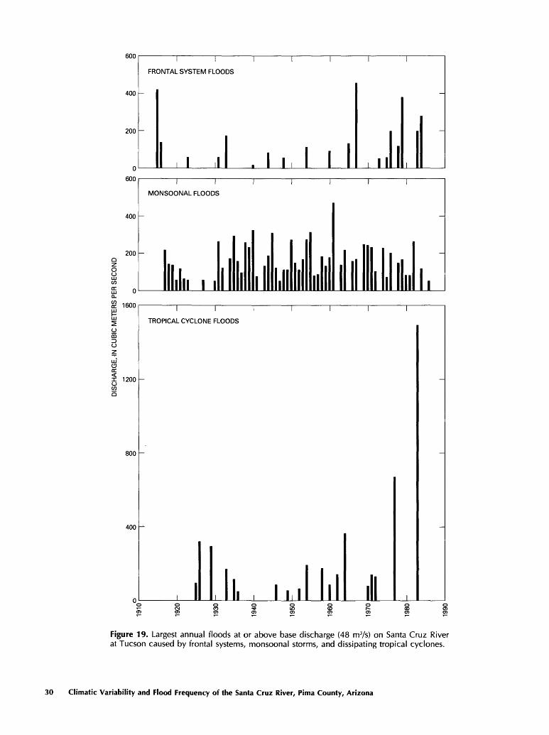
< 5'

cr -<r a> Q.

o 8. n .a c n I o

Table 8. Floods above base discharge, by storm type, Santa Cruz River at Tucson, Arizona

[Base discharge, 48 m3/s. Hydroclimatic water year, November 1 to October 31]

Floods caused by

Frontal storms

Date

12-23-14 1-20-16

1 1-17-73 ...2-16-31 8-21-33 9-15-44 9-77-48

9-24-54 1-12-60

1 '"i O^ £*GL

i *~) ^r\ f*^

3-14-73 9-13-75 0-75-76 _

i n o i 7817 10 787-04-83

12-28-84

Discharge, in cubic

meters per second

- 425..... 142

SB

SO

- 17387

- 55 - 114..... 91 - 137..... 456

..... 60----- 201

118

ICO

----- 1700oei

Dissipating tropical cyclones

Date

9 1 8 OS

9 OO ^f.

9-24 29 9-21-33 8-24-35

8 no if.

10-01-46 -9-10-49

7-20-54 7 ">Q co

9-10-60 9-26-62 9-10-64 9-05-70

8 1 1 7 1

10-19-72 10-10-77 i n m 01

Discharge, in cubic

meters per second

..... 96 - 323

- 173- 117..... 49..... 84 - 56

..... 191i en

..... 84

..... 141o/ro

81

- 133..... 671-- 1,493

Date

9-08-17

8 m 1 e

8 m 1 o

8 no on

8 ni 017 T7 T7

8 1 7 11

9 m 97

8 m in

8-10-31 7 in n

8 TJ 7/1

9-01-35

7 r\s -isr

7-10-37

8 nc ie8-03-39 8-14-40

Discharge, in cubic

meters per second

----- 212..... 139 - 133 - 55----- 113..... 57----- 54 - 55----- 50

r\s i

----- 119----- 170----- 292----- 153----- 93

- 227

Monsoonal storms

Date

8-14-41

8-16 44 8-10-45 8 04-46

8-16-48 8-08-49 7-30-50

8 m c.1

8 1 £. GL^

Q ni cc

7 70 Sfi

8-31-57 7-70-58 _

8 7O SO

Discharge, in cubic

meters per second

..... 71i oe1 8C

- 306..... 121..... 48..... 109

me----- 269----- 142

me..... 167 - 271

} f\C\

..... 740£

1 en ~ 125

Date

8-10-60

8 T5 £i1

8 r\f ST*}

7-24-64 8-19-66 7-17-67 8-06-69 7-20-70 8-17-71 7-15-72 7-08-74 7-12-75 9-25-76

8 m 78

8 1 C. 7Q

8 1 1 en7 07 01

8 01 09

8-14-84

7 *-) 1 O£

Discharge, in cubic

meters per second

..... 1 74

..... 470__ 1 32 - 2 14 - 156..... 166..... 247 - 242 - 227

QQ

__ 225..... 70 - 201----- 142

1 /d7O

..... 76 - '260 - 1 13 - 50

'Estimated.

The censored data for each hydroclimatic type of flood on the Santa Cruz River (table 9) were fit to the three- parameter log-Pearson type III distributions using maximum- likelihood analysis. The method of moments was not used because reliable estimates of the mean, variance, and skew of censored data are more efficiently made using maximum- likelihood analysis (Pollard, 1977, p. 245-246). Techniques used to fit type I censored data to probability distributions using maximum-likelihood techniques were presented by Stedinger and Cohn (1986, 1987). Stedinger and Cohn (1986) developed a maximum-likelihood function, L, for the com­ bination of conventional gage and historical data. Because no historical data are used for the Santa Cruz River at Tuc­ son, the likelihood function has to be slightly modified from those given in Stedinger and Cohn (1986) and Stedinger and others (1988). The likelihood function, LN, for nonexceedances of base discharge is

(2)

where= population mean,= population standard deviation,

y = the population skew coefficient,F(Xt) = the cumulative-density function, andXh = logarithm (base 10) of the base discharge.

The likelihood function for discharges that exceed base discharge is

^.y)=n [/(*,-)]> (3)

where/(*.) = the probability-density function, and x = an array of the logarithms of floods that exceed

base discharge.The total likelihood function is

(4)

Because equation 4 is maximized over (j., a, and y and the maximum of the logarithm of the likelihood func­ tion, In L, occurs at the same place as the maximum for the likelihood function, L, equation (4) becomes

lnL(ji, a, y) = (h - n}ln[F(xb )] + I ln[/(*,.)]. (5)

Hydroclimatic Flood-Frequency Analysis of the Santa Cruz River 31

Table 9. Floods above base discharge, by storm type, Santa Cruz River at Cortaro, Arizona

[Base discharge, 76 m3/s. Hydroclimatic water year, November 1 to October 31]

Floods caused by

Frontal storms

Date

1 9.3 1-40

9-16-44

Q- 1 0-46 - -

3-23-54 _

in 9e so

1-12-60 i f\ Tl £.£

1 O O1 til

9-22-73 --3 f\9 TC

19 1C 7B

9 99 fi 1

9-11-82

9-04-83

Discharge, in cubic

meters per

second

----- 482

----- 122

..... 79

70

..... 79

..... 176

..... 476

__ 104

..... 222

----- 533

..... 122

..... 190

01^

Dissipating tropical cyclones

Date

7-16-54

7 9Q SR

9-26-62

9 1 0-64 - -

9-06-70

10-19-72

10-10-77 i rv r\9 B3

9-06-84

Discharge, in cubic

meters per

second

- 173

~i(\£.

317

..... 450

136

- 255

- 651

O7

Date

8-14-40

8-08-41

9-24-43

8-16-44

8-10-45

8-04-46

8-15-47

7-30-50

7-25-51

8-14-52

7-14-53

7-24-54

8-03-55

7-29-56

9-01-57

Discharge, in cubic

meters per

second

- 482

..... 170

----- 156

- 160

- 397

..... 126

----- 213

- 365

- 193

----- 173

- 306

- 259

- 470

CO

- 125

Monsoonal storms

Date

8 1 9 Sfi

8 9f\ SO

8-11-60

8-16-84

8-23-61

8 r\f /-o

9-06-64

7-16-65

8-19-66

7-17-67

8-06-69

7-20-70

8 9n 71

8-12-72

7-08-74

Discharge, in cubic

meters per

second

----- 227

1 S9

__ 14fi

- 416

- 205

__ 203

..... 77

..... 169

- 163T^O

- 317

9SB

9OO

- 331

Date

7-12-75

9-25-76

9-10-77

8 n9 ~?B

7-25-81

8 97 C9

8 m B"}

Discharge, in cubic

meters per

second

..... 147"3nn

----- 133

..... 79

- 377

..... 176

Equation 5 is iteratively maximized by finding the point where 3(ln L)/|i, 3(ln L)/3o, and 3(ln L)/3y equal zero (Stedinger and others, 1988). Details of the numerical meth­ ods used to maximize equation 5 are given in Stedinger and Conn (1986), Cohn (1986), and Stedinger and others (1988).

Mixed-population analysis is a method used to com­ bine different populations of floods that may occur in a gaging record to estimate annual recurrence intervals for that river (Kite, 1988, p. 6-7). Distinct populations can be combined in several ways. One approach for estimating the cumulative density function, Fr from m separate cumula­ tive density functions, F., is given by Waylen and Woo (1982) as

FT (x<x]=f[Fi (x<x]. (6)

This approach is difficult using maximum-likelihood analysis, because F would have to be differentiated and substituted into equations 2, 3, and 5 for solution. A simi­ lar method given by Kite (1988) and Crippen (1978) sim­ ply uses the assumption of independence of the populations to estimate the exceedance probability of occurrence. For two populations, the composite exceedance probability, PT, is estimated using

(7)

where P l (X>x) and P2(X>x) are the exceedance probabili­ ties of the independent populations. Jarrett and Costa

(1988) showed an example of two-population mixed- population analysis for Colorado. A third population can be introduced to produce

(8)

By substituting l/T for P and rearranging, the annual recurrence interval for the mixed population, Ta, can be esti­ mated as three populations described by T{ , T2 , and r3 from

r = TTTZ

(T, T.+T. T^+T.T~T-T-T+ 1)(9)

Frequency of Floods Caused by Different Storm Types

Three scenarios of flood frequency were analyzed for the Santa Cruz River at Tucson. First, probability distributions were fit to all data for annual floods caused by each storm type (fig. 19). The moments of the fitted distribution are given in table 10. Flood- frequency relations (fig. 20) show the relative impor­ tance of each storm type to annual flood frequency. Floods caused by monsoonal storms dominate flood fre­ quency for recurrence intervals of less than 10 years. Floods caused by tropical cyclones dominate flood fre­ quency at recurrence intervals above 20 years. Al­ though the frequency of floods caused by frontal systems never dominates (fig. 20), it parallels that for

32 Climatic Variability and Flood Frequency of the Santa Cruz River, Pima County, Arizona

tropical cyclones up to the 10-year recurrence interval, at which point the two relations diverge. The relation for the Santa Cruz River at Cortaro is similar.

The relations shown in figure 20 do not represent an accurate statistical analysis of flood frequency on the Santa Cruz River. As is apparent for floods caused by tropical cyclones and frontal systems, the frequency of floods caused by storm types is dependent on the period of record that is considered (fig. 19). Use of data from all periods for each storm type violates the assumption that a homogeneous population is being analyzed. The annual flood frequency for this scenario (fig. 20) is probably meaningless because flood frequency appears to exhibit weak stationarity of order 1. For comparative purposes, the

100-year flood estimated from a mixed-population analysis is 1,050 m3/s at Tucson and 1,610 m3/s at Cortaro.

To obtain stationary series for analysis, the assump­ tion was made that populations of floods caused by frontal systems, dissipating tropical cyclones, and monsoonal storms are derived from different populations for 1930-59 and 1960-86. At Cortaro, only flows for 1960-84 were analyzed because only 18 years of data are available be­ fore 1960. The relations for floods at Tucson caused by different storm types that occurred after 1960 appear in figure 21. The same general relations occur as in figure 20, but discharges for given recurrence intervals are larger for the post-1960 relations (fig. 21). Comparison of the es­ timated mean, standard deviation, and skew coefficients

1000

100

10

1 I

EXPLANATION

ANNUAL FLOODS

D TROPICAL CYCLONE FLOODS

O FRONTAL SYSTEM FLOODS

O MONSOONAL STORM FLOODS

1.05 1.25 2 5 10

RECURRENCE INTERVAL, IN YEARS

20 50 100 200

Figure 20. Mixed-population analysis of floods caused by different storm types between 1915 and 1986, Santa Cruz River at Tucson, Arizona. Probability distributions were fit using invalid assumptions; curves are presented for illustrative purposes only.

Hydroclimatic Flood-Frequency Analysis of the Santa Cruz River 33

for post-1960 floods with those estimated for the entire record (table 10) suggests the reason for the increase. Al­ though the mean discharge decreases for post-1960 floods at Tucson caused by tropical cyclones and monsoonal storms, the variances for all types increase. The skew coefficient becomes more negative (table 10), but because it is poorly estimated, changes in the skew coefficient are not considered significant. From mixed-population analy­ sis, the annual 100-year flood for Santa Cruz River at Tuc­ son is 1,660 m3/s after 1960 (fig. 21). At Cortaro, the annual 100-year flood is 2,030 m3/s after 1960. Both esti­ mates are strongly affected by the large flood of October 1983.

Results for floods at Tucson for 1930 59 caused by tropical cyclones and frontal systems (fig. 22) contrast

with the post-1960 results; floods caused by monsoonal storms dominate flood frequency. Although the means for floods caused by tropical cyclones and frontal systems are similar for 1930-59 and post-1960 (table 10), the standard deviations are much less for 1930-59 than post-1960. For 1930-59, the annual 100-year flood is 323 m3/s and is es­ sentially the frequency of floods caused by monsoonal storms (fig. 22).

The results of the hydroclimatic flood-frequency analysis underscore the cause for the increased flood fre­ quency on the Santa Cruz River. The probability for floods caused by dissipating tropical cyclones, frontal systems, and, to a lesser extent, monsoonal storms changed in the 20th century. The greatest difference among the distribu­ tions estimated for 1930-59 and 1960-86 is the increased

----- n TROPICAL CYCLONE FLOODS AFTER 1960

O FRONTAL SYSTEM FLOODS AFTER 1960

O MONSOONAL STORM FLOODS AFTER 1960

1000 -

100

10

EXPLANATION

ANNUAL FLOODS AFTER 1960

I_____I1.05 1.25 2 5 10

RECURRENCE INTERVAL, IN YEARS

20 50 100 200

Figure 21. Mixed-population analysis of floods caused by different storm types between 1960 and 1986 for the Santa Cruz River at Tucson, Arizona.

34 Climatic Variability and Flood Frequency of the Santa Cruz River, Pima County, Arizona

Table 10. Statistics for annual series of floods caused by three storm types for the Santa Cruz River at Tucson and Cortaro, Arizona

[Statistics were generated by fitting floods above base discharges of 48 and 76 m 3/s for the Tucson and Cortaro stations, respectively, using maximum- likelihood analysis]

Floods caused by storm type

Mean logarithm

of discharge

Santa Cruz River at Tucson,

Tropical cyclones after 1960 Frontal systems after 1960 Monsoonal storms after 1 960 Tropical cyclones, 1930-59 - Frontal systems, 1930-59 Monsoonal storms, 1 930-59

1.264 1.007 2.068

.730 1.133 1.979 .586 .800

2.130

Standard deviation

of log discharge

Arizona

0.865 1.118 .327

1.596 1.297 .423

1.442 1.002 .298

Coefficient of skew of log

discharge

-0.4001 1 IT,

Q£~C

- .040 - .639 -.948

- .639 - .501 - .401

Santa Cruz River at Cortaro, Arizona

Tropical cyclones after 1 960 Frontal systems after 1960 ~ Monsoonal storms after 1960

.523 2.427 2.214

.778 1.218 2.147

1.651 .884 .313

1.675 1.296 .335

.9481119

1.080-1.112 -1.639 -1.174

variance and, in the case of floods caused by tropical cy­ clones and monsoonal storms, more negative skew coeffi­ cients. Because estimates of long-recurrence interval floods are heavily influenced by higher-order moments, the 100-year flood estimate for 1960-86 is more than four times larger than that for 1930-59 for the Santa Cruz River at Tucson.

The main problem with the hydroclimatic flood- frequency analysis is the inability to assign uncertainty es­ timates to discharges at given recurrence intervals. A method is not available for estimating standard errors or confidence limits for cumulative-distribution functions using mixed-population analysis. Variances for the floods caused by different storm types, however, are high, and the maximum length of a stationary period is only 30 years. For example, the uncertainty in the 100-year flood estimates from hydroclimatic-frequency analyses would be expected to be higher than for frequency analyses using a longer period of record, such as the 71-year annual flood series for Santa Cruz River at Tucson (fig. 2).

A second problem results from the assumption that floods during periods are derived from a stationary popula­ tion. Climatic information suggests that transitions among periods may have been gradual instead of abrupt (fig. 10). The assumption of stationarity within periods is required to obtain estimates of population parameters, and no com­

pelling evidence indicates problems with stationarity within the periods.

Finally, use of the hydroclimatic flood-frequency analyses requires an assessment of which period best rep­ resents future climatic conditions. Although no evidence was found to suggest that the conditions for 1960-86 have changed, the maximum length of periods examined in this study is only 30 years. The question of whether future conditions will be similar to 1930-59 or 1960-86 is im­ possible to answer at this time. It is also questionable that a meaningful 100-year discharge can be estimated from an annual flood series of only 30 years.

SUMMARY AND CONCLUSIONS

The effects of climatic variability on the annual flood series and flood-frequency estimates were evaluated for the Santa Cruz River at Tucson and Santa Cruz River at Cor­ taro. Previous estimates of the 100-year flood at Tucson, calculated using different techniques and assumptions, ranged from 572 to 2,780 m3/s. This discrepancy has been attrib­ uted to increasing flood magnitudes caused by channelization and land-use changes in the last two decades. The magni­ tude of the 100-year flood for Santa Cruz River at Tucson, calculated from a log-Pearson type III distribution using the method of moments, increased from 577 to 872 m3/s when annual peak discharges between 1970 and 1986 were in­ cluded in the calculations. Flood-frequency estimates for the Santa Cruz River are strongly influenced by an extraor­ dinary flood in October 1983, but it is also true that six of the seven largest floods at Tucson occurred after 1960. In addition, the seasonality of annual floods changed signifi­ cantly after 1960; whereas floods in summer accounted for 97 percent of annual peaks between 1930 and 1959, floods in summer accounted for 61 percent of annual peaks be­ tween 1960 and 1986. Although changes in land use and channelization may have affected the magnitude of annual floods, climatic variability is identified as the main cause for the change in flood frequency.

The annual flood series at Tucson exhibits weak stationarity of order 1. Analyses for 1915-29, 1930-59, and 1960-86 showed that the mean does not change sig­ nificantly; however, the variance and skew coefficient change significantly with time. Trend analyses revealed no trends in the annual flood series or among periods of the series. Trend analyses, however, are intended to detect changes in the mean instead of the variance. Changes in variance, which were detected in nonparametric tests, exert a heavy influence on estimates of long-recurrence interval floods such as the 100-year discharge.

In southern Arizona, fluctuations in large-scale oce­ anic and atmospheric processes are reflected in the sea­ sonal distribution of precipitation and increased probability of large floods. Twentieth-century climatic variability

Summary and Conclusions 35

stems from decadal trends in atmospheric circulation over the Northern Hemisphere and in the frequency of El Nino- Southern Oscillation (ENSO) phenomena in the equatorial Pacific Ocean. Before 1930 and after 1960, westerly winds on average followed a more meridional path, and ENSO conditions occurred more frequently and with greater vari­ ability in the equatorial Pacific. By contrast, the westerlies followed a more zonal flow, and ENSO conditions oc­ curred less frequently with less variability between 1930 and 1960. Meridional circulation and the climatology associated with ENSO conditions enhance Tucson precipi­ tation in the winter, spring, and fall and possibly reduce summer rainfall.

Seasonal discharge on the Santa Cruz River is simi­ larly related to climatic variability. Winter and fall floods account for 53 percent of annual peaks before 1930, only 3

percent from 1930 to 1959, and 39 percent after 1960. Changes in flood frequency on the Santa Cruz River are attributed to the changing probabilities of floods caused by certain storm types. In particular, the joint occurrence of cutoff low-pressure systems and tropical cyclones in­ creases the probability for large floods along the Santa Cruz River. This joint occurrence tends to occur more fre­ quently during ENSO years and during 1960-86.

Using procedures of the Interagency Advisory Com­ mittee on Water Data (1982), flood frequency at Tucson was estimated for the entire record using years with ENSO conditions and years with non-ENSO conditions. Climatic analyses suggest that the flood-producing mechanisms are not strictly stationary in the 20th century; therefore, analy­ ses that require the assumption of stationarity may be in­ valid. Assuming stationarity for the entire record, the

1000

100

I I I

EXPLANATION

ANNUAL FLOODS, 1930-1959

O TROPICAL CYCLONE FLOODS, 1930-1959

O FRONTAL SYSTEM FLOODS, 1930-1959

O MONSOONAL STORM FLOODS, 1930-1959

1C 1.05 1.25 2 5 10

RECURRENCE INTERVAL, IN YEARS

20 50 100 200

Figure 22. Mixed-population analysis of floods caused by different storm types between 1930 and 1959 for the Santa Cruz River at Tucson, Arizona

36 Climatic Variability and Flood Frequency of the Santa Cruz River, Pima County, Arizona

100-year flood is estimated to be 872 m3/s. Assuming stationarity, the 100-year floods for years with ENSO and non-ENSO conditions are estimated to be 1,300 and 628 m3/s, respectively. The frequency analysis for the entire record and for ENSO years is strongly affected by the un­ usually large flood of October 1983.

The frequency of floods caused by the three general storm types summer monsoonal storms, frontal systems, and dissipating tropical cyclones was estimated using maximum-likelihood analysis and the log-Pearson type III distribution. Annual flood frequency was estimated by as­ suming independence of the three types of floods and using a three-population mixed-population analysis. Floods caused by dissipating tropical cyclones determine the annual flood frequency at recurrence intervals greater than about 20 years for all years and for 1960-86. For 1930-59, floods caused by monsoonal storms dominate flood frequency for all re­ currence intervals. Assuming stationarity, which analyses of climate suggest is invalid, the 100-year flood for all years is 1,050 m3/s (table 7). The 100-year flood for 1960-86 is estimated to be 1,660 m3/s and was strongly affected by the flood of October 1983. Likewise, the 100-year flood for 1930-59 was estimated to be 323 m3/s (table 7). These analyses do not have an estimated uncertainty; however, the uncertainty is expected to be high because of short record length and high variance.

The results of flood-frequency analyses presented in this study raise questions about the validity of applying statistical flood-frequency analysis to the Santa Cruz River. Frequency analysis requires the assumptions of interannual independence and stationarity, neither of which are totally valid for the Santa Cruz River. Separation of the record into ENSO and non-ENSO conditions creates two independent populations but does not solve the prob­ lem of a variance that changes with time. Separation of floods by storm type assumes three independent, stationary populations, although long-recurrence-interval floods are estimated from stationary records of 30 years or less. Also, judicious use of the mixed-population results requires an assessment of future climatic conditions, which is ques­ tionable. Finally, separation of periods requires the as­ sumption that climatic shifts are abrupt, whereas the climatic data presented in this report indicate that shifts may be gradual. Inclusion of the flood of October 1983 also adds to the complexity of the problem. Although this flood was the largest since at least 1891 and ordinarily would have been treated as a historic peak (Interagency Advisory Committee on Water Resources, 1982), consider­ ations of stationarity prevented extension of a historical record length for this flood.

Flood-frequency estimates for the Santa Cruz River need to be used cautiously in design applications. Other methods, such as rainfall-runoff models (Ponce and others, 1985), may be appropriate alternatives to flood-frequency analysis. Frequency analysis, however, is appropriate in

certain circumstances. For example, because ENSO condi­ tions demonstrably affect flood frequency on the Santa Cruz River, flood plains could be managed for a specified recurrence interval of floods during ENSO conditions. Therefore, an appropriate estimate of the 100-year flood would be 1,300 m3/s at Tucson. A similar scenario could be developed for floods caused by dissipating tropical cy­ clones. However, the period of record would have to be selected that best represents future or design conditions.

Perhaps the best estimate for the 100-year flood is obtained by assuming that future climate may be similar with that of 1960-86. This assumption may be valid for the immediate future but is tenuous when conditions for several decades into the future are considered. Given this assumption, an appropriate magnitude for the 100-year flood is 1,660 m3/s at Tucson (table 7).

REFERENCES CITED

Aldridge, B.N., 1970, Floods of November 1965 to January 1966 in the Gila River basin, Arizona and New Mexico, and adjacent basins in Arizona: U.S. Geological Survey Water-Supply Paper 1850-C, 176 p.

Aldridge, B.N., and Eychaner, J.H., 1984, Floods of October 1977 in southern Arizona and March 1978 in central Ari­ zona: U.S. Geological Survey Water-Supply Paper 2223, 143 p.

Aldridge, B.N., and Hales, T.A., 1984, Floods of November 1978 to March 1979 in Arizona and west-central New Mexico: U.S. Geological Survey Water-Supply Paper 2241, 149 p.

Andrade, E.R., and Sellers, W.D., 1988, El Nino and its effect on precipitation in Arizona: Journal of Climatology, v. 8, p. 403^10.

Baker, V.R., 1984, Questions raised by the Tucson flood of 1983: Journal of the Arizona-Nevada Academy of Sciences, v. 14, p. 211-219.

Balling, R.C., and Lawson, M.P., 1982, Twentieth century changes in winter climatic regions: Climatic Change, v. 4, p. 57-69.

Barry, R.G., Kiladis, G., and Bradley, R.S., 1981, Synoptic cli­ matology of the western United States in relation to cli­ matic fluctuations during the twentieth century: Journal of Climatology, v. 1, p. 97-113.

Betancourt, J.L., 1990, Tucson's Santa Cruz River and the ar- royo legacy: Tucson, University of Arizona, doctoral dis­ sertation, 239 p.

Betancourt, J.L., and Turner, R.M., 1988, Historic arroyo-cutting and subsequent channel changes at the Congress Street crossing, Santa Cruz River, in Whitehead, E.E., Hutchinson, C.F., Timmermann, B.N., and Varady, R.G., eds., Arid lands today and tomorrow: Boulder, Colorado, Westview Press, p. 1353-1371.

Boughton, W.C., and Renard, K.G., 1984, Flood frequency characteristics of some Arizona watersheds: Water Re­ sources Bulletin, v. 20, p. 761-769.

Box, G.E.P., and Jenkins, G.M., 1971, Time series analysis: San Francisco, Holden-Day, 553 p.

References Cited 37

Bradley, R.S., Diaz, H.F., Kiladis, G.N., and Eischeid, J.K., 1987, ENSO signal in continental temperature and precipi­ tation records: Nature, v. 327, p. 497-501.

Burkham, D.E., 1981, Uncertainties resulting from changes in river form: American Society of Civil Engineers, Journal of the Hydraulics Division, v. 107, p. 593-610.

Carleton, A.M., 1986, Synoptic-dynamic character of "bursts" and "breaks" in the south-west U.S. summer precipitation singularity: Journal of Climatology, v. 6, p. 605-623.

1987, Summer circulation climate of the American Southwest, 1945-1984: Annals of the Association of American Geographers, v. 77, p. 619-634.

Cayan, D.R., 1986, North Atlantic seasonal sea surface tem­ perature anomalies and associated statistics: La Jolla, Cali­ fornia, Scripps Institution of Oceanography, SIO Reference No. 85-19, 89 p.

Cohn, T.A., 1986, Flood frequency analysis with historical flood information: Ithaca, New York, Cornell University, doctoral dissertation, 144 p.

Conover, W.J., 1971, Practical nonparametric statistics: New York, John Wiley, 493 p.

Cooke, R.U., and Reeves, R.R., 1976, Arroyos and environ­ mental change in the American Southwest: Oxford, En­ gland, Oxford University Press, 213 p.

Crippen, J.R., 1978, Composite log-type III frequency- magnitude curve of annual floods: U.S. Geological Survey Open-File Report 78-352, 5 p.

Cross, R.L., 1988, Eastern North Pacific hurricanes, 1987: Mariners Weather Log, v. 32, p. 12-16.

Diaz, H.F., and Quayle, R.G., 1980, The climate of the United States since 1895, Spatial and temporal changes: Monthly Weather Review, v. 108, p. 249-266.

Douglas, A.V., 1974, Cutoff lows in the southwestern United States and their effects on precipitation of this region: Tucson, Arizona, Laboratory of Tree Ring Research, Final Report on Department of Commerce Contract 1-35241 No. 3, 40 p.

Douglas, A.V., Cayan, D.R., and Namias, Jerome, 1982, Large- scale changes in North Pacific and North American weather patterns in recent decades: Monthly Weather Re­ view, v. 110, p. 1851-1862.

Douglas, A.V., and Englehart, P.J., 1984, Factors leading to the heavy precipitation regimes of 1982-1983 in the United States, in Proceedings of the Eighth Annual Cli­ mate Diagnostics Workshop: Washington, D.C., National Oceanic and Atmospheric Administration, p. 42-54.

Dunne, Thomas, and Leopold, L.B., 1978, Water in environ­ mental planning: San Francisco, W.H. Freeman, 818 p.

Durrenberger, R.W., and Wood, Richard, 1979, Climate and energy in the Tucson region: Tempe, Arizona State Uni­ versity, Laboratory of Climatology report, 90 p.

Dzerdzeevskii, B.L., 1969, Climatic epochs in the twentieth century and some comments on the analysis of past climates, in Wright, H.E., Jr., ed., Quaternary geology and climate, v. 16 of the Proceedings of the 7th Congress, In­ ternational Quaternary Association: Washington, D.C., National Academy of Sciences Publication 1701, p. 49- 60.

- 1970, Circulation mechanisms in the atmosphere of the Northern Hemisphere in the 20th century: Moscow, Insti­

tute of Geography, Soviet Academy of Sciences, trans­ lated from the Russian by R. Goedecke, 361 p.

Eidemiller, D.I., 1978, The frequency of tropical cyclones in the southwestern United States and northwestern Mexico: Arizona State Climatologist, Climatological Publications, Scientific Papers 1, 41 p.

Elliott, W.P., and Angell, J.K., 1988, Evidence for changes in Southern Oscillation relationships during the last 100 years: Journal of Climate, v. 1, p. 729-737.

Enfield, D.B., 1989, El Nino, past and present: Reviews of Geophysics, v. 27, p. 159-187.

Eychaner, J.H., 1984, Estimation of magnitude and frequency of floods in Pima County, Arizona, with comparisons of alternative methods: U.S. Geological Survey Water-Re­ sources Investigation 84-4142, 69 p.

Federal Emergency Management Agency, 1982, Flood insur­ ance study, city of Tucson, Arizona, Pima County: Wash­ ington, D.C., Federal Emergency Management Agency, 45P-

1986, A unified national program for floodplain man­ agement: Washington, D.C., Federal Emergency Manage­ ment Agency, Interagency Task Force on Floodplain Management, p. A-l to D-12.

Folland, C.K., Palmer, T.N., and Parker, D.E., 1986, Sahel rainfall and worldwide sea temperatures, 1901-85: Nature, v. 320, p. 602-606.

Granger, O.E., 1984, Twentieth-century climate anomaly pat­ terns over the southwestern United States: Physical Geog­ raphy, v. 5, p. 164-185.

Hales, J.E., Jr., 1974, Southwestern United States summer monsoon source, Gulf of Mexico or Pacific Ocean?: Weatherwise, v. 24, p. 148-155.

Hansen, E.M., and Schwarz, F.K., 1981, Meteorology of im­ portant rainstorms in the Colorado River and Great Basin drainages: National Oceanic and Atmospheric Administra­ tion Hydrometeorological Report 50, 167 p.

Hansen, E.M., Schwarz, F.K., and Riedel, J.T., 1977, Prob­ able maximum precipitation estimates, Colorado River and Great Basin drainages: National Oceanic and Atmo­ spheric Administration Hydrometeorological Report 49, 161 p.

Hirsch, R.M., 1987, Probability plotting position formulas for flood records with historical information: Journal of Hy­ drology, v. 96, p. 185-199.

Hirsch, R.M., and Stedinger, J.R., 1987, Plotting positions for historical floods and their precision: Water Resources Re­ search, v. 23, p. 715-727.

Hirschboeck, K.K., 1985, Hydroclimatology of flow events in the Gila River Basin, central and southern Arizona: Tuc­ son, University of Arizona, doctoral dissertation, 335 p.

1987, Catastrophic flooding and atmospheric circulation anomalies, in Mayer, Larry, and Nash, David, eds., Cata­ strophic flooding: Boston, Alien and Unwin, p. 23-56.

1988, Flood hydroclimatology, in Baker, V.R., Kochel,R.C., and Patton, P.C., eds., Flood geomorphology: New York, John Wiley, p. 27^9.

Hjalmarson, H.W., 1987, Discussion Large basin determinis­ tic hydrology A case study: American Society of Civil Engineers, Journal of the Hydraulics Division, v. 113, p.1461-1463.

38 Climatic Variability and Flood Frequency of the Santa Cruz River, Pima County, Arizona

1990, Flood of October 1983 and history of flooding along the San Francisco River, Clifton, Arizona: U.S. Geological Survey Water-Resources Investigations Report 85-4225-B, 42 p.

Horel, J.D., and Wallace, J.M., 1981, Planetary scale atmo­ spheric phenomena associations with the Southern Oscil­ lation: Monthly Weather Review, v. 109, p. 813-829.

Interagency Advisory Committee on Water Data, 1982, Guide­ lines for determining flood flow frequency: Washington, D.C., Interagency Advisory Committee on Water Data, Hydrology Subcommittee, Bulletin 17B, 28 p.

Jarrett, R.D., and Costa, J.E., 1988, Evaluation of the flood hydrology in the Colorado Front Range using precipita­ tion, streamflow, and paleoflood data for the Big Thomp­ son River basin: U.S. Geological Survey Water-Resources Investigations Report 87-4117, 37 p.

Kalnicky, R.A., 1974, Climatic change since 1950: Annals of the Association of American Geographers, v. 64, p. 1 GO- 112.

Keith, S.J.S., 1981, Stream channel recharge in the Tucson Basin and its implications for groundwater management: Tucson, University of Arizona, Master's thesis, 84 p.

Kiladis, G.N., and Diaz, H.F., 1989, Global climatic anoma­ lies associated with extremes in the Southern Oscillation: Journal of Climate, v. 2, p. 1069-1090.

Kite, G.W., 1988, Frequency and risk analyses in hydrology, 4th edition: Littleton, Colorado, Water Resources Publi­ cations, 257 p.

Knapp, F.C., 1937, Report on Santa Cruz watershed: Tucson, Arizona, U.S. Department of Agriculture, Soil Conserva­ tion Service, unpublished report, 37 p.

Lewis, D.D., 1963, Desert floods A report on southern Ari­ zona floods of September 1962: Arizona State Land De­ partment Water-Resources Report 13, 30 p.

Lins, H.F., 1985, Streamflow variability in the United States, 1931-78: Journal of Climate and Applied Meteorology, v. 24, p. 463-471.

Maddox, R.A., Canova, Faye, and Hoxit, L.R., 1980, Meteoro­ logical characteristics of flash flood events over the western United States: Monthly Weather Review, v. 108, p. 1866- 1877.

Malvick, A.J., 1980, A magnitude-frequency-area relation for floods in Arizona: Tucson, University of Arizona, Engi­ neering Experimental Station, Research Report 2, 25 p.

Mooley, D.A., and Parthasarathy, B., 1984, Fluctuations in all India summer monsoon rainfall during 1871-1978: Climatic Change, v. 6, p. 287-301.

Namias, Jerome, 1986, Persistence of flow patterns over North America and adjacent ocean sectors: Monthly Weather Re­ view, v. 114, p. 1368-1383.

Namias, Jerome, Yuan, X., and Cayan, D.R., 1988, Persistence of North Pacific sea surface temperature and atmospheric flow patterns: Journal of Climate, v. 1, p. 682-703.

National Oceanic and Atmospheric Administration, 1988, Daily weather maps: National Oceanic and Atmospheric Adminis­ tration, 8 p.

Nicholls, N., 1988, El Nino-Southern Oscillation and rainfall variability: Journal of Climate, v. 1, p. 418-421.

Ojo, Oyediran, 1987, Rainfall trends in West Africa, 1901-1985, in Solomon, S.I., Beran, M., and Hoff, W., eds., The influ­

ence of climate change and climatic variability on the hydrologic regime and water resources: International Asso­ ciation of Hydrological Sciences Publication No. 168, p. 37-43.

Pollard, J.H., 1977, A handbook of numerical and statistical techniques: Cambridge, England, Cambridge University Press, 349 p.

Ponce, V.M., Osmolski, Zbig, and Smutzer, David, 1985, Large basin deterministic hydrology, a case study: Journal of Hy­ draulic Engineering, American Society of Civil Engineers, v. Ill, p. 1227-1245.

Pyke, C.B., 1972, Some meteorological aspects of the seasonal distribution of precipitation in the western United States and Baja California: Los Angeles, University of California, Water Resources Center Contribution No. 139, 205 p.

Quinn, W.H., Neal, V.T., Antunez de Mayolo, S.E., 1987, El Nino occurrences over the past four and a half centuries: Journal of Geophysical Research, v. 92, no. C13, p. 14449- 14461.

Rasmusson, E.M., 1967, Atmospheric water vapor transport and the water balance of North America, part 1, Characteristics of the water vapor flux field: Monthly Weather Review, v. 95, p. 403-426.

1984, El Nino, the ocean/atmosphere connection: Oceanus, v. 27, p. 5-12.

1985, El Nino and variations in climate: American Scien­ tist, v. 73, p. 168-177.

Reich, B.M., 1984, Recent changes in a flood series: Journal of the Arizona-Nevada Academy of Science, v. 14, p. 231- 238.

Reich, B.F., and Davis, D.R., 1985, The 1983 Santa Cruz flood How should highway engineers respond?: Transportation Research Board Record, v. 1017, p. 1-7.

1986, Reluctance to increase the regulatory flood on a degrading river: Phoenix, Arizona, Association of State Floodplain Managers, Inc., Proceedings of Seminar, "Im­ proving the effectiveness of floodplain management in arid and semiarid regions", May 24-26, p. 99-102.

Reitan, C.H., 1960, Distribution of precipitable water vapor over the continental United States: Bulletin of the Ameri­ can Meteorological Society, v. 41, p. 79-87.

Reiter, E.R., 1983, Surges of tropical Pacific rainfall and tele- connections with extratropical circulation patterns, in Street-Perrott, F.A., Beran, M., and Ratcliff, R., eds., Variations in the global water budget: Dordrecht, Nether­ lands, D. Reidel, p. 285-299.

Reyes, Sergio, and Cadet, D.L., 1988, The southwest branch of the North American monsoon during 1979: Monthly Weather Review, v. 116, p. 1175-1187.

Roeske, R.H., 1978, Methods for estimating the magnitude and frequency of floods in Arizona: Arizona Department of Transportation ADOT-RS-15-121, 82 p. [Also available as NTIS report PB289 424].

Roeske, R.H., Garrett, J.M., and Eychaner, J.H., 1989, Floods of October 1983 in southeastern Arizona: U.S. Geological Survey Water-Resources Investigations Report 85-4225-C, 77 p.

Ropelewski, C.F., and Halpert, M.S., 1986, North American precipitation and temperature patterns associated with El Nino-Southern Oscillation (ENSO): Monthly Weather Re-

References Cited 39

view, v. 114, p. 2352-2362.Ropelewski, C.F., and Jones, P.O., 1987, An extension of the

Tahiti-Darwin Southern Oscillation Index: Monthly Weather Review, v. 115, p. 2161-2165.

Rosendal, H.E., 1962, Eastern North Pacific tropical cyclones, 1947-1961: Mariners Weather Log, v. 6, p. 195-201.

Saarinen, T.F., Baker, V.R., Durrenberger, Robert, Maddock, Thomas, Jr., 1984, The Tucson, Arizona, flood of October 1983: Washington, D.C., National Academy Press, 112 p.

Schwalen, H.C.. 1942, Rainfall and runoff in the upper Santa Cruz River drainage basin: Tucson, University of Arizona, Agricultural Experiment Station Technical Bulletin No. 95, p. 421-472.

Sellers, W.D., 1960, Precipitation trends in Arizona and west­ ern New Mexico: Proceedings, 28th Annual Western Snow Conference, Santa Fe, New Mexico, p. 81-94.

Sellers, W.D., and Hill, R.H., eds., 1974, Arizona climate, 1931-1972: Tucson, University of Arizona Press, 616 p.

Slezak-Pearthree, M., and Baker, V.R., 1987, Channel change along the Rillito Creek system of southeastern Arizona, 1941 through 1983: Arizona Bureau of Geology and Mineral Technology Geological Survey Branch, Special Paper 6, 58P-

Smith, Walter, 1986, The effects of eastern north Pacific tropi­ cal cyclones on the southwestern United States: National Oceanic and Atmospheric Administration Technical Memorandum NWS WS-197, 229 p.

Stedinger, J.R., and Conn, T.A., 1986, Flood frequency analy­ sis with historical and paleoflood information: Water Re­ sources Research, v. 22, p. 785-793.

1987, Historical flood frequency data: Its value and use, in Singh, Vijay, ed., Flood frequency and risk analysis: Boston, D. Reidel, p. 273-286.

Stedinger, J.R., Surani, Rafiq, and Therivel, Riki, 1988, Max us­ ers guide, A program for flood frequency analysis using

systematic-record, historical, botanical, physical paleohy- drologic and regional hydrologic information using maxi­ mum-likelihood techniques: Ithaca, New York, Cornell University Department of Environmental Engineering, 51 p.

Tang, M., and Reiter, E.R., 1984, Plateau monsoons of the northern hemisphere A comparison between North America and Tibet: Monthly Weather Review, v. 112, p. 617-637.

Thomas, W.O., Jr., 1985, A uniform technique for flood- frequency analysis: Journal of Water Resources Planning and Management, v. Ill, p. 321-337.

Troup, A.J., 1965, The Southern Oscillation: Quarterly Journal of the Royal Meteorological Society, v. 91, p. 490-506.

U.S. Army Corps of Engineers, 1972, Interim report on a survey for flood control, Santa Cruz River Basin: Los Angeles, U.S. Army Corps of Engineers Report, 43 p.

U.S. Water Resources Council, 1981, Guidelines for determining flood flow frequency: Hydrology Subcommittee Bulletin 17B, 183 p.

Waylen, Peter, and Woo, Ming-Ko, 1982, Prediction of annual floods generated by mixed processes: Water Resources Re­ search^. 18, p. 1283-1286.

White, N.D., and Garrett, W.B., 1987, Water resources data, Arizona, water year 1984: U.S. Geological Survey Water- Data Report AZ-84-1, 381 p.

Wilson, R.P., and Garrett, W.B., 1989, Water resources data, Arizona, water year 1987: U.S. Geological Survey Water- Data Report AZ-87-1, 385 p.

Wright, P.B., 1984, Relationships between indices of the South­ ern Oscillation: Monthly Weather Review, v. 112, p. 1913- 1919.

Yarnal, B., and Diaz, H.F., 1986, Relationships between ex­ tremes of the Southern Oscillation and the winter climate of the Anglo-American Pacific Coast: Journal of Climatology, v. 6, p. 197-219.

40 Climatic Variability and Flood Frequency of the Santa Cruz River, Pima County, Arizona