Embed Size (px)
Citation preview
1
Climate system change, from global to local:
Lake Winnipeg Watershed
Review on regulation of Lake Winnipeg
Prepared for the Manitoba Clean Environment Commission
By Paul Henry Beckwith
April 1st, 2015
https://wpgwaterandwaste.files.wordpress.com/2015/02/lake_winnipeg.jpg
2
Table of Contents
Table of Contents ................................................................................................................... 2
Introduction ............................................................................................................................ 3
Overview: Abrupt climate change ........................................................................................... 4
Global climate system context ................................................................................................ 6
Arctic albedo decline (terrestrial snow cover, sea ice, and Greenland); temperature
amplification ........................................................................................................................ 9
Arctic methane emission increases (from marine sediments and terrestrial permafrost),
global warming potential, regional radiative forcing ............................................................13
Effect of the decline of the equator-to-Arctic temperature gradient on the general circulation
and extreme weather patterns ............................................................................................18
Tipping elements of the global climate system ...................................................................21
Global summary ....................................................................................................................23
Local Lake Winnipeg Effects .................................................................................................24
Figures ..................................................................................................................................26
Glossary ................................................................................................................................42
Key web links ........................................................................................................................43
References ............................................................................................................................44
3
Introduction
In 2008 Lenton et al. assessed potential tipping elements in the climate system,
including Arctic sea-ice, Greenland and West Antarctic ice sheets, Amazon and boreal forests,
monsoons, permafrost, and methane hydrates. This report will discuss some key aspects of the
most vulnerable elements, including those that seem to be most rapidly changing, potentially
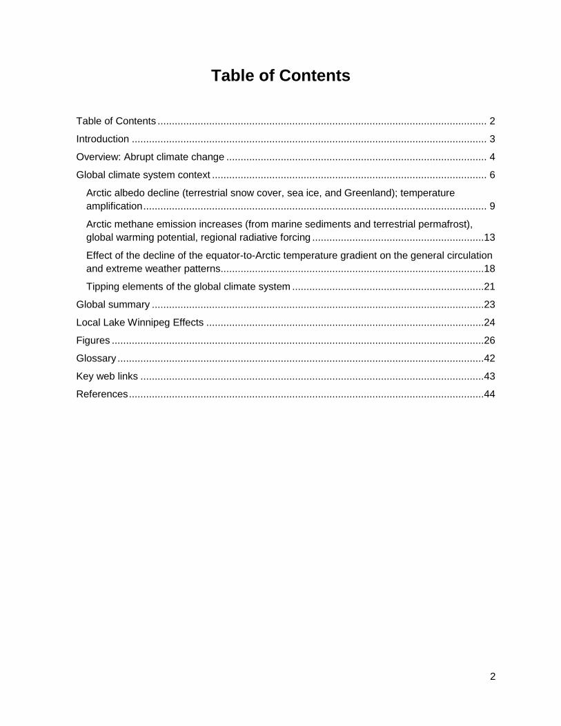
causing cascading effects. Implications to the local scale, specifically to the Lake Winnipeg
Watershed will also be examined.
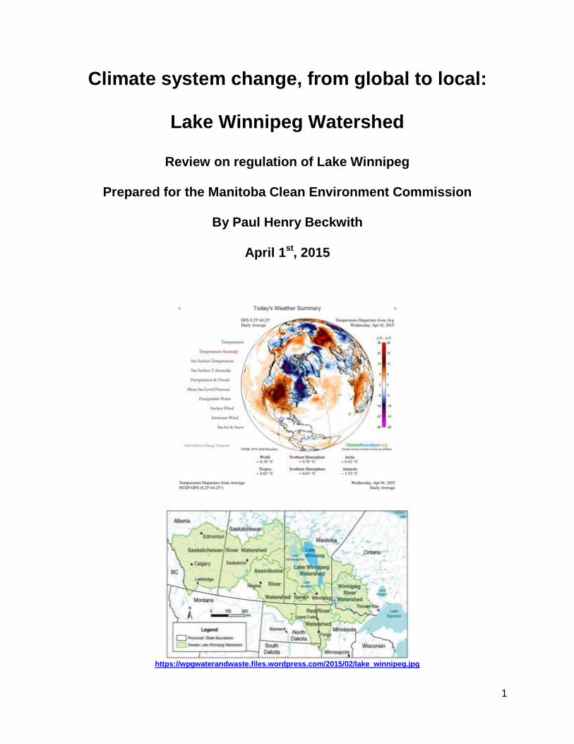
Over the last few years it has become increasingly evident that the climate system on
the Earth is changing in a nonlinear fashion. Rapidly rising anthropogenic greenhouse gas
emissions from fossil fuel combustion and land use changes (Figure 1) are causing significant
global warming (IPCC AR5 WG1 to 3, 2013 and 2014; also see Figures 2 and 3). Large positive
feedbacks (see glossary explanation), for example in the Arctic from increased solar absorption
due to greatly decreasing albedo from reduced sea ice (Figures 4 and 5), Greenland melt ponds
(Figure 6), and terrestrial snow cover (Figure 7) are significantly amplifying atmosphere and
ocean warming, resulting in large Arctic methane emissions from thawing terrestrial and marine
permafrost, most noticeably over the Eastern Siberian Arctic Shelf and in other shallow marine
regions (Figure 8, terrestrial permafrost map in Figure 9). In addition there is an increase in
storm frequency, intensity, and duration leading to increased coastal erosion in the Arctic.
Combined, these feedback effects are warming the Arctic at rates that are 4 to 5 times greater
than the global average temperature rise. The greatly reduced equator-to-pole temperature
gradient acts, in a climatological sense, to slow the jet stream winds and this should influence
Rossby wave properties including increasing amplitude, changing spatial location, wavelength
and symmetry (Francis and Vavrus, 2012); also see Figures 10 and 11. This in turn would
increase the frequency, severity, duration, and spatial range of extreme weather events such as
flooding, heat waves, and droughts (Hansen et. al., 2012). In addition, it causes “weather
whiplashing”, which are rapid jumps in temperature (hot to cold and vice versa) and/or
precipitation (drought to flood and vice versa); for example see Figure 12. Examples of torrential
rain events in Canada include Calgary flooding (Figures 13 and 14) and Toronto flooding. An
extensive heat wave event killed more than 70,000 people in Europe in 2003 (Figure 15). More
recently, extensive heat over Lake Erie caused and explosion of algae that shut down the
Toledo water supply (Figure 16). These weather extremes will be greatly amplified if the late
summer sea ice cover completely vanishes within the next few years. However, most climate
models have under-projected the rates of change being observed (see Figure 5), for example
they project summer sea ice vanishing between 2040-2070 (IPCC AR4, 2007; AR5, 2013) while
extrapolating from measurements strongly suggest that this will happen before 2020 (see Figure
4). Model projections for methane release from Arctic sources suggest negligible emissions this
century (IPCC AR4, 2007; IPCC AR5, 2013; NRC, 2013) while near real-time satellite data is
showing large rises in methane levels in the Arctic are occurring even today (see Figure 8).
4
Overview: Abrupt climate change
There have been many times in the history of the Earth when regional (as well as global)
temperatures have changed extremely quickly (nonlinearly, even abruptly) relative to the much
more common incremental (linear) change periods (Alley et al. 2003, Chapman Conference
2009, Cronin 2009, IPPC AR5 2013, NRC report 2013). For example, during Dansgaard-
Oeschger (DO) oscillations in the last ice age between 70 to 30 ka (1 ka = one thousand years
ago) there were up to 29 abrupt warmings in which the temperature over Greenland as
determined from proxy ice core records typically rose in the range of 5 to 10 oC (from glacial
conditions at roughly -30 oC up to -20 oC) on a timescale of two decades or less (Singh et. al,
2013). The largest amplitude DO event had a temperature rise of 16 oC (Lang et al. 1999).
There were also rapid rises of temperature with correspondingly rapid rises of global sea level
during the Younger Dryas (YD), the last interglacial (Eemian), as well as during the Paleocene-
Eocene Thermal Maximum (PETM) (Cronin, 2009). In Hansen et al., 2007 there is an extensive
review on contemporary climate change and positive feedbacks and sensitivity of climate to
forcings which can move the climate quickly between different states.
Contemporary global climate system change
As a Phd candidate at the university of Ottawa, and part time professor, my teaching and
research focus is in abrupt climate change.
My working research hypothesis is outlined as follows: We are presently in the very early
stages of an abrupt climate change transition, at least for some elements of the climate system,
most notably those in the Arctic region. Greenhouse gas (GHG) levels have increased in
magnitude and rate (IPCC AR5, 2013; also see Figure 1) enough to rapidly melt large areas of
the Arctic sea ice (Figures 4 and 5), Greenland (Figure 6) and terrestrial snow cover (Figure 7)
to greatly reduce the albedo resulting in larger solar absorption in the region. This in turn is
causing significant Arctic amplification of temperature rates of change as compared to the global
mean temperature rates of change (Figures 2 and 3). Therefore the equator-to-north-pole
temperature gradient is greatly reduced. Thermodynamic heat flow considerations (heat moves
from hot areas to cold areas) necessitate a reduction in the amount of heat transported
northward from the equator to the Arctic via both the atmospheric circulation and ocean
circulation patterns. Lower volume flow rates northward (in the atmosphere and oceans) leads
to decreased wind speeds in high altitude jet streams and/or a spatial narrowing of the jet
stream cross sectional area. It also leads to an increase in the meridional amplitude of the
Rossby wave (jet streams) in the Northern Hemisphere (NH), and likely more fragmentation
(filimentation) as well as changes in the number and location of the pressure ridges and troughs
(Figures 10 and 11). Since the latitudinal pressure gradient force (PGF) has decreased with the
temperature gradient reduction, the land/ocean temperature contrasts have larger relative
influence on the atmospheric circulation pattern, and the jet streams have an increased
tendency to larger amplitude blocking events with longer duration (persistence). Since heat flow
from the equator northward is divided into roughly 2/3 atmospheric and 1/3 ocean (Srokosz et
al., 2012), the atmospheric changes are the most significant. However there is also a reduction
5
in ocean currents (including the Atlantic Ocean Gulf Stream and the Pacific Ocean Kuroshio
Current). Combined with the elevated water vapor content of the atmosphere from increased
evaporation with global average temperature rise (rising exponentialy with temperature
according to the Clausius-Clapeyron equation; approximated to roughly 7% per oC for small
temperature change) (Peixoto and Oort, 1992) these atmospheric circulation changes may be
leading to more extreme weather events, most notably to torrential downpours (Coumou and
Rahmstorf, 2012; IPCC SREX, 2012). Examples of this in Canada are Calgary in June, 2013
(Figures 13 and 14) and Toronto in July, 2013.
The Arctic amplification is also leading to increasing amounts of methane emissions in
the northern region (from terrestrial permafrost (Marshall, 2013; see Figure 9 for Canadian
permafrost map) and marine sources (ocean floor embedded permafrost and marine clathrates)
(Shakova et al., 2010, 2013)), contributing to rising global methane levels and higher regional
forcing in the Arctic further amplifying the warming (see Figure 8). As the Arctic albedo
continues to decrease in the next few years with declining sea ice area, decreasing terrestrial
snow cover area, and decreasing Greenland ice cap reflectance from melt ponds and old ice
exposure, my view is that the frequency, intensity, duration, and spatial extent of these extreme
weather events will continue to increase perhaps as high as an order of magnitude (based on
the increased radiative forcing). Effects on human civilization and well-being would be very
significant under this scenario as climate instability increased. More specifically, there would be
immediate threats to global food supply, city and rural infrastructure, and loss of global
biodiversity with species extinctions as well as increased ocean acidification. This would
certainly cause great economic hardships and national conflicts and wars over ever scarcer
resources. It is becoming increasingly obvious to ever larger numbers of the public and scientific
communities that our global weather patterns are rapidly changing at rates that are
unprecedented in human experience. System stability can no longer be taken for granted.
The mainstream scientific consensus view as summarized by the IPCC AR5 document
that was released in late September, 2013 provides a comprehensive view of relatively recent
scientific thinking on climate change (up to April, 2011; since the peer reviewed paper cutoff
date for AR5 was April, 2013 and a paper has to have been published for two years to be
included). Although this extensive body of work determines that the probability of human caused
global warming occurring is now >95%, it still has the conclusion that the methane emissions
from the Arctic and other regions is growing slowly, and will continue to grow slowly for the
forseable future (over the next century) even in the worst case IPCC scenario RCP8.5
(Representative Concentration Pathway with 8.5 W/m2 of ERF (Enhanced Radiative Forcing) by
2100) considered in the CMIP5 (Climate Model Intercomparison Project V study). As far as
extreme weather events go, the document recognizes increases and provides an update on the
interim SREX document on this topic (IPCC SREX, 2012). However, connections between the
increasing levels of extreme weather and increased rates of Arctic albedo reduction are not
considered, and thus a short-term ramping up of such events as albedo ramps down is not
considered in any of the CMIP5 models in the report.
6
Examining the overall tipping elements of the climate system, Lenton et al., 2008 used
expert panel judgement to categorize relative risks, timescales of change, and effects. An even
more recent document titled “Abrupt Impacts of Climate Change, Anticipating Surprises” (NRC,
2013) expanded on a previous document titled “Abrupt climate change: Inevitable surprises”
(NRC, 2002) and considers that methane emissions will not rise significantly enough over the
next century to cause abrupt climate change, although the document does consider a higher
risk of WAIS (Western Antarctic Ice Sheet) collapse leading to greatly elevated GMSL (Global
Mean Sea Level) rates of rise. There is clearly disagreement in the literature regarding the
importance of near-term methane changes in the climate system.
Global climate system context
Rapidly increasing anthropogenic fossil fuel combustion, as well as changing land use
practices and industrial growth are rapidly accelerating growth in concentrations of atmospheric
greenhouse gases (GHGs), most notably for carbon dioxide (CO2), methane (CH4), and nitrous
oxide (N2O), as shown in Figure 1. These greenhouse gases (having recently reached 400 ppm,
1850 ppb, and 325 ppb, respectively at Mauna Loa) are at concentrations much higher than
upper limits of their previously narrow ranges (180 to 280 ppm, 350 to 750 ppb, and 200 to 280
ppb, respectively) for at least the last 800,000 years as measured from Antarctic ice sheet ice
core records (and confirmed back to 120,000 years in Greenland ice core records) (IPCC AR5,
2013). Higher levels of GHGs are trapping more long-wave radiation (heat) in the climate
system and are warming the atmosphere and oceans. According to Ramanathan and Feng,
2008 the measured increase in GHG since the preindustrial era has very likely committed the
Earth to a warming of 2.4 oC (1.4 oC to 4.3 oC) above the preindustrial era. Since removal of
anthropogenic CO2 from the atmosphere by natural processes alone would take many
hundreds-of-thousands of years, the warming is essentially irreversible on human timescales
(IPCC AR5 WG1, 2013) unless emissions are halted and methods are used to remove CO2
from the atmosphere (for example by accelerating the sink rates); collectively these methods
are categorized under Carbon Dioxide Removal (CDR).
Accelerated increases in temperatures in the Arctic region appear to be causing large
structural system element changes. Arctic sea ice cover and terrestrial snow cover have rapidly
declined; from 1979 to 2012 the snow cover area (Figure 7) has lost an average -17.6% per
decade (Derksen and Brown, 2012) while the sea ice cover area has decreased an average of -
10% per decade (varying between -13% per decade in September and -2.6% per decade in
March) (Perovich et al, 2012). Recently, a new record low in Arctic sea ice area was set in the
summer melt season ending September 16th, 2012 representing a decline of 18% relative to the
previous record low in 2007 (49% below the long term average from 1979 to 2000). Year-to-
year variability appears to be increasing with the declining sea ice area trend (Figures 4 and 5).
Positive feedbacks in the Arctic, mainly from the declining albedo due to collapse of highly
reflective sea ice and snow cover (replaced by dark ocean water and permafrost, respectively)
have caused an amplification of warming in the high Arctic by factors of 4x to 5x (Lesins, 2012,
2013); also see Figures 2 and 3.
7
Further acceleration in Arctic rates of warming are presently occuring as methane
concentrations in the Arctic region are rapidly rising. Specific sources include terrestrial
permafrost rapidly thawing due to increased shortwave radiation absorption and thus heating
due to the absence of high albedo snow cover, most notably the Yedoma region in Siberia
(Vonk et al., 2013). In the last year, methane caused craters have been discovered in northern
Siberia (likely from thawing methane clathrates). High levels of methane have also been
measured along Arctic coastal permafrost regions as increased wave action and larger storm
surges due to stronger, more frequent and longer duration polar cylones in the newly opened
Arctic ocean are inundating shallowly sloping coastlines and causing increased erosion rates
(Gunther, 2013a,b). Also, the oceans over shallow continental shelves in the region are
warming significantly causing perforations in the sea floor sediment layers releasing large area
plumes of methane, most notably over the East Siberian Arctic Shelf (ESAS) (Shakova et al.,
2010, 2013). Methane surges are also observed from deeper waters (Ruppel, 2011). Direct
flask measurements at weather stations in Svalbaard and Barrow (ESRL data) and remote
sensing satellite measurements (AIRS data, IASI data) have detected large methane
concentrations throughout the Arctic.
On the global scale methane concentration levels have experienced an increase since
2007 (see Figure 1), reflecting a change from the prior leveling out trend (ESRL data). Outside
of the Arctic, methane emissions have been measured on continental shelves off the
southeastern U.S. seaboard (Brothers et al., 2012) that are warming due to the Gulf Stream
shift closer to the coastline. Destruction of wetlands, increases in rice production (Archer, 2010)
and increased global energy dependence on fracking for natural gas in shales and sediments
are also contributing significantly rising global methane levels (Tollefson, 2013). Since the global
warming potential of methane is about 150x that of carbon dioxide over timescales of a few
years (IPPC AR5, 2013), the significance of methane is increasing rapidly.
The importance of the accelerated Arctic warming at rates up to 4x to 5x larger than
global average temperature increase cannot be underestimated; what happens in the Arctic
does not stay in the Arctic. Since the equator mean annual temperature has a very small
variation (mean temperature changes < 3 oC seasonally), and the increase in temperature from
climate change is relatively small there (most of the increase in energy there goes into latent
heat from increased evaporation of the oceans), the equator-to-Arctic temperature gradient
rapidly decreases. This reduces the equator-to-pole pressure gradient (from basic meteorology);
and results in a smaller thermodynamic driving force (which moves heat from warm regions like
the equator to cold regions like the poles, proportionately to the temperature gradient) (Barry
and Chorley, 2010; Peixoto and Oort, 1992). The net result from the Arctic warming via
decreased albedo (increased absorption of shortwave radiation) is that less heat moves from
the equator to the Arctic region; via both the atmosphere and oceanic circulation patterns.
In the atmosphere, when a stationary air parcel is acted on by a PGF (Pressure Gradient
Force; arising from a temperature gradient) it accelerates until it reaches geostrophic flow (PGF
= Coriolis force). As this flow moves to higher latitudes there is geographic constriction in cross-
section, and increases in speed enhanced by conservation of total vorticity (angular momentum
8
in a fluid) and the increasing Coriolis force (which is zero at the equator, and increases with
latitude to a maximum at the pole) deflecting it to the right (in the northern hemisphere) (Peixoto
and Oort, 1992). The net result is the formation of jet streams. When the temperature gradient is
reduced (either from seasonal change or Arctic amplification) there is a smaller northward heat
transport so the northern hemisphere jet streams have smaller volume flow rates Q (m3/s); to
preserve angular momentum they generally move southward. Smaller Q means a smaller
(velocity) x (cross-sectional area) product, so the jets can narrow and/or decrease speed and/or
become broken up and/or change latitude. As Q decreases, the land/ocean temperature
contrast and land topography become more important (even dominant) factors in jet stream
behaviour, and as these Rossby waves respond they tend to distort and have higher amplitudes
(become more meridional) and thus more easily locked to the fixed continental-ocean
geography in the northern hemisphere. Thus, blocking becomes more persistent (Woolings et
al., 2012; Francis et al., 2013; Overland et al., 2013).
The spatial and temporal characteristics of the high altitude jet streams play a crucial
role in controlling and guiding weather patterns (Barry and Chorley, 2010). In the boreal summer
with a warmer northern hemisphere from higher solar zenith angles (thus higher solar
intensities) the cold air does not extend as far south and therefore the jet streams are located
closer to the pole. At the present time, albedo feedbacks are rapidly reducing this volume of
cold air in the Arctic. In the boreal winter, as the volume of cold air in the Arctic increases the
equator-to-pole temperature gradient increases and the jet streams move roughly twice as fast,
on average. However, with Arctic temperature amplification primarily from summer albedo
reduction (less sea-ice means a larger area of dark ocean water which can absorb more solar
radiation, thus much more heat is stored during the summer melt season). With the seasonal
change from summer to fall and then winter, large amounts of heat escape from the warmer
oceans leading to disruption of the polar vortex (jetstreams become more meridional (wavy),
average eastward velocity decreases and more flow fragmentation (namely there are large
width and velocity variations). Thus, the weather patterns which are guided along the jetstreams
are changed (extreme weather events like torrential rains increase in frequency, severity,
duration, and vary in spatial extent from the norm). In addition, there is now 4% more water
vapor in the atmosphere now than there was 3 decades ago (7% per oC x 0.6 oC of warming);
this is due to the increased evaporation levels from a rising global average temperature and the
increased ability of warmer air to hold more water (from Clausius-Clapeyron equation) (Peixoto
and Oort, 1992). The extra water vapor in the atmosphere is providing large amounts of latent
heat energy to fuel more massive and intense storms. The slower jet streams are indicative of
slower storm advection. Coumou and Rahmstorf, 2012 have suggested that these two factors,
combined, are causing increasing frequencies, amplitudes, durations, and changing spatial
extents of many severe weather events, leading for example to torrential rains and subsequent
floods, long duration droughts leading to crop failures, and also more derechos and haboobs;
however attribution research is in early stages. An increase in heat wave extremes has been
statistically confirmed for summer (June, July, August) by Hansen et al., 2012a. For example,
this extremely wavy Rossby wave pattern of jets resulted in patterns like the low pressure
trough for a month causing Pakistan flooding in the summer of 2010 (70% of country flooded)
simultaneously with the blocking high pressure ridge over Moscow causing a record heat wave
9
with record forest fires causing a loss of 40% of the Russian grain crop and up to 50,000
fatalities (Coumou and Rahmstorf, 2012). Similar persistent jet stream activity is associated with
the recent southwestern U.S. drought, and was directly responsible for the redirection of
Hurricane Sandy to make an unprecedented left turn and impact the New Jersey and New York
coastal regions (Beckwith, 2012b; Livescience, 2013).
For the duration of Earth’s history the climate system has undergone both linear and
nonlinear changes. Linear changes, in which incrementally larger forcings (internal or external to
the system) cause a given system element to respond by reconfiguring with incrementally larger
proportionate responses is the most frequent system behavior. Non-linear changes, in which a
given forcing results in the system element responding disproportionately larger are usually
much less frequent, and very difficult to anticipate in advance. Each specific system element
responds to the forcing with its own characteristic response time, which is typically hours to
days with the atmosphere and months to years to centuries or even millennia with the oceans
and cryosphere, and even longer (geological timescales) with the lithosphere. However there
are thresholds (tipping points; birfurcation points) in most systems. When a threshold or “tipping
point” is crossed by either a large forcing or by the cumulative buildup of many small
incremental forcings then the system can respond with a surprisingly large and unexpected
change (relative to linear changes) that is disproportionate to the forcing. This nonlinear or
abrupt change (regime shift) usually eventually leads to a new stable state (in which linear
changes again become the norm). Contemporary changes in various elements of the climate
system (such as Arctic albedo decline, methane emission increase) are occuring at rates faster
than linear due to positive feedback effects.
In the records of past climates, in which temperature and rainfall and other climate
parameters are obtained from various proxies such as pollen records, tree rings, ice cores on
Greenland and Antarctica, and marine sediments, among others, it is very clear that there have
been many rapid or abrupt transitions in temperature and precipitation. Some causes of
extremely rapid changes (D-O oscillations, YD) have been attributed to a switch on (or off) in the
global ocean current pattern known as the Atlantic Meridional Overturning Circulation (AMOC)
(Broecker, 2010). Others (PETM) have been attributed to large sudden emissions of methane
from the ocean floor hydrates (Kennett et al., 2003).
It is essential that we understand how quickly the changes in the Earth climate system
can occur and learn about the type of climate regimes that we can end up reaching within a
decade or two if we experience an abrupt climate change transition. For example, is the climate
of the Earth heading to a much warmer overall state in which snow and ice in the Arctic regions
becomes a distant memory? If so, then can societal adaptation adjust to the rapid rates of
change, and can mitigation be utilized to slow the changes?
Arctic albedo decline (terrestrial snow cover, sea ice, and Greenland); temperature amplification
10
The most sensitive elements of the climate system seem to be located in the Arctic
region and consist of a) sea ice volume and b) thickness (PIOMAS, and CryoSat-2 data (Laxon
et al., 2013)), c) sea ice extent (NSIDC data) and d) area (Cryosphere Today), e) sea ice
motion, specifically at export regions (U.S. Navy data), and f) terrestrial snow cover area, mostly
in the boreal spring (Rutgers University Global Snow Lab data (Derksen and Brown, 2012).
Other physical measurements that affect ice melt, such as ocean temperature and salinity with
depth, ocean currents, and regional meteorology will also be examined in relation to other
variables. The overall decline in Arctic albedo, mainly from sea ice and snow cover area
reductions, but also from Greenland albedo decrease (Box et al., 2012, 2013) will be studied in
relation to the associated known feedbacks (mostly positive).
While some research suggests that the albedo effect of the Arctic terrestrial snow cover
decline is roughly equivalent to that of the Arctic summer sea ice decline (Flanner et al., 2011),
more recent work (Tang et. al., 2013) finds that the sea ice effect on atmospheric jet streams is
larger. The present consensus on Arctic sea ice decline based on CMIP5 modeling projections
and ERF forcing scenarios (RCP2.6, RCP4.5, RCP6.0, and RCP8.5) from the IPCC AR5 (2013)
report are consistent with the results of CMIP3 model projections from IPCC AR4, 2007. The
basic conclusion is that the Arctic sea ice will not vanish completely (at least to an area < 1
million km2) for the first time (i.e., near the end of the melt season in September) for at least 30
years or longer (2040 to 2070). However, observations from the summer 2012 melt season
indicated that the ice extent reached record lows, and the pattern of decline recorded from data-
model hybrids (PIOMAS) conflicts strongly with this view, suggesting that the ice extent may
become < 1 million km2 before the end of this decade. This view is gaining traction via continued
monitoring of Arctic sea ice volume data and by results from a higher-resolution Regional
Climate Model (RCM) applied in the Arctic (Maslowski et al., 2012) in contrast to the lower-
resolution IPCC AR5 Global Climate Models (GCMs). The RCM suggests that the sea ice will
first vanish within a very short time (2016 3 years). Recent Cryosat-2 satellite measurements
of sea ice thickness (Laxon et al., 2013) adds credibility to this rapid sea ice loss scenario. Of
course negative feedbacks which are not currently identified may affect this prediction, flattening
out the current downward trend. Possibilities may include a) open water and thin ice freezes
faster than thick ice, and b) thinner ice spreads more increasing albedo, and c) marine cloud
cover increases with more open water, leading to cooling.
A main objective of ongoing Arctic research is to put more accurate bounds on the
potential date of loss of essentially all sea ice in the Arctic Ocean (ranging from about 2016 per
Maslowski et al., 2006, 2012) to the decades 2040 - 2070 per IPCC AR5. In conjunction with
Arctic terrestrial snow cover reduction (mostly in the spring), this is decreasing the albedo of the
Arctic region (which has already decreased from 52% to 48% between 1979 and 2011
according to a Scripps Institute study of CERES satellite data
http://www.nasa.gov/content/goddard/nasa-satellites-see-arctic-surface-darkening-
faster/index.html#.U_TmbPldV8E.
Overall Arctic changes can also be examined in a top-down Arctic climate system
approach. Climate changes in the Arctic are larger and faster than anywhere else on the planet.
11
There are many interacting processes and elements that are changing, and clearly these need
to be researched in detail. However, to understand the system, and the importance of sea ice
and snow cover decline, it is important to understand the fundamentals of these changes. For
example, during the record breaking 2012 summer melt season an extremely rare and very
large cyclone churned over the Arctic ocean region in early August (from Aug. 2nd to 10th) and
the ice was shredded into smaller (larger surface area) chunks, and transported out into the
open Atlantic ocean via the Fram Strait. Within the Arctic basin near the North Pole, the ice was
fractured and melted very quickly due to ocean mixing whereby warmer, saltier water from
cyclone churning was brought up from 500m depths (as measured by tethered ocean buoys) to
displace the fresher and colder surface melt water surrounding the ice near the surface. In
addition, the extremely deep central pressures of the cyclone caused a storm surge by pulling
up the surface level of the water by about 30 cm across a large portion of the region resulting in
larger inward flows of warmer Pacific water (through the Bering Strait) and warmer Atlantic
water (from the Norwegian Sea and between Iceland and Svalbard). Also, the duration of the
cyclone was 10 days which is unusually long for such a storm, however research suggests the
potential for Arctic cylones to last up to 30 days duration with increased warming of the region
(Zhang et. a., 2004). The storm maintained power via injection of sensible heat energy from
Siberia which had 20 oC high temperatures and large concentrations of soot and ash from large
area forest fires burning at that time in the high north. Also, the storm was constrained to the
Arctic Ocean basin. As it started to head southward out of the basin the large rightward
deflection from the strong Coriolis force (maximized right at the North Pole) caused it to curve
continuously to the right and head back to the central part of the basin again, in a meandering
circular loop. To further compound the melting, incoming fresh water flows from the major
Siberian rivers into the Arctic Ocean basin contributed greatly to melting due to their elevated
temperatures and large flow rates sourced from amplified land warming resulting in large
terrestrial snow melt. Atmospheric data for the region to analyze these effects can be obtained
from NCEP reanalysis. The frequency, amplitude, duration, and spatial extent of cyclones has
been increasing in the Arctic and northern hemisphere mid-latitude regions over the last several
decades. The nonlinear loss of sea ice volume is occurring for every month of the year, not just
in the boreal summer months. If the ice indeed leaves the Arctic ocean in a summer before
2020 (for a month or less) then the next two warmest months (August and October) may trend
to zero within a year or two later, followed by another two months (November and July) within
about 3 or 4 years. Calculations by Wadham’s (personal communication) and others suggest
that radiative forcing by sea ice is about 0.1 W/m2 now, will triple when the ice is gone for a few
months, and will be 7x when the ice is gone for half the year. Arctic ice behavior in 2013 was
unprecedented in March (from Satellite images) with significant and widespread cracking at the
time of usual maximum strength, but the summer minimum had more ice than in 2012, as did
2014. In March 2015 the winter sea ice maximum extent set a record low; it is clear that there is
great variability and many records are being broken.
As the ice rapidly vanished during the boreal summer in 2012 (reducing area and
thickness) the ocean water heating rates increased at all depths. For example, water over the
relatively shallow (maximum depth 50 m) ESAS (Eastern Siberia Arctic Shelf) warmed with
temperature anomalies typically in the range of 3 to 5 oC (maximum measured 7 oC) resulting in
12
perforations of the frozen marine sediments and increases in methane emission ebullition
through the water column (Shakova et al., 2013). Methane emission changes in the Arctic are
discussed in the next section and can be a strong feedback.
Albedo reduction is the strongest feedback thus far. As fast as the sea ice decline trends
are (namely a 49 % area loss over 3 decades or so) (from PIOMAS data, and CryoSat-2 data
published in Laxon et al., 2013), with a mean loss of 12 % per decade it was still superceded by
terrestrial snow coverage loss (18.7 % per decade in the time period from 1979 to 2010)
(Derksen and Brown, 2012). These large rates of decline of highly reflective terrestrial snow
cover and sea ice area (albedos above 80 % or so (snow and ice), being replaced with albedos
less than 30 % (exposed ground) or less than 10 % (dark sea water)) are collapsing the regional
albedo. Greenland melt is also lowering albedo, although the area is lower (compared to sea
ice loss and snow cover loss) so the effect is smaller. Thus, the increased absorption of
shortwave solar radiation in the region causes large warming anomalies over extended periods
of time. For example, Greenland underwent an exceptional and unprecedented reduction in
albedo over the space of 4 days in July, 2012. The area percentage of the ice cap undergoing
surface melt increased from 40% of the Greenland ice cap to 97% within these 4 days, which
was an incredibly abrupt change in its own right given the high altitude of the peak (3275 m).
Albedo of the Greenland cap dropped significantly due to increased meltwater pooling on the
surface, exposure of entrained dirt and soot in the ice, and possible increased levels of soot and
ash deposition from Siberian fires being sucked into the cylonic type storm systems. In fact
Greenland ice melt rates are estimated in a recent paper to have increased about 5x between
the mid-1990s and the present (Shepherd et al., 2012); this represents a doubling rate of <7
years. Finally, the rapid tropospheric warming of the Arctic atmosphere is allowing less
stratospheric heating such that in 2010 there was an unprecedented 40% drop in Arctic ozone
concentrations (Manney et al., 2011). For the first time in the ozone record, the Arctic ozone
hole size and magnitude rivaled that of the yearly ozone hole that forms in the much colder
Antarctic stratosphere. This part of the study aims to put the overall Arctic changes into a more
global context.
In summary, the Arctic sea ice and spring snow cover are both trending strongly
downward. While the global temperature increase has slowed over the last 15 years or so, the
warming of the Arctic in recent years is much faster than anticipated (AMAP, 2009, 2012).
Other Arctic feedback effects (based on ice motion, fracturing behavior, cyclone frequency and
severity, ocean temperatures and salinity) need to be researched. What is clear is that the Arctic
amplification (warming in Arctic versus global warming average) was as large as 4x over the last
3 decades (Screen et al., 2012) and is primarily due to the decline in albedo of terrestrial snow
cover area and sea ice area (Screen et al., 2010). This resulted in an albedo feedback radiative
forcing of 0.3 to 1.1 W/m2 based on observations (Flanner et al., 2011). With further decline we
can calculate the additional radiative forcing in the region (for both albedo, as well as for
methane emissions) to determine the overall additional Arctic amplification effects. It is expected
that this Arctic amplification will change many aspects of the climate outside of the region,
including atmospheric circulation patterns, vegetation, and the carbon cycle and have large
impacts in and beyond the Arctic (Serreze and Barry, 2011). What is not known is how quickly
13
these changes will occur, the magnitude of the changes, and the effects on the overall climate
system.
Arctic methane emission increases (from marine sediments and terrestrial permafrost), global warming potential, regional radiative forcing
Methane emissions in the Arctic originating from terrestrial permafrost (Vonk et al., 2013)
and marine ocean sediments, most notably on the shallow continental shelves such as the very
large East Siberian Arctic Shelf (ESAS) (Shakanova et al., 2013), as well as from marine
methane clathrates (both shallow and deep) are being observed.
The Arctic region stores about 33% of all the carbon held within the global terrestrial
ecosystem, and roughly 40% of the carbon that is present globally in near-surface soils (AMAP,
2009). Large quantities of methane hydrate (methane trapped in the center of a frozen lattice of
water) exist on the ocean floor and buried within the ocean sediments, kept in a stable state by
high water pressure and low temperatures (for example at 0 oC and 200 m water depth
(personal communication with Archer, 2013)). These are considered to be vulnerable to ocean
and associated sediment warming (AMAP, 2009). According to the latest IPCC AR5 WG1, 2013
report, the amount of methane stored in the Arctic hydrates could be >10x the methane that is
presently in the global atmosphere, and the Arctic permafrost (terrestrial and marine) holds >2x
the amount of carbon present in the atmosphere today. This vast carbon storage could
potentially be released as either CO2 or CH4 (depending on location O2 level), and act as very
large positive feedbacks causing even larger warming upon release. It is estimated that the
Arctic is presently a source of from 3% to 9% (15 Tg (Gt) to 50 Tg) of the global net emissions
of methane from land and ocean (AMAP, 2009). Arctic marine emissions of methane are
thought to be roughly 1/3 of that emitted from wetlands in the Arctic tundra (Shakova et al., 2010
and McGuire et al., 2012). The various factors controlling the seasonality of the methane
emissions from high-Arctic tundra have been examined in Mastepanov et al, 2013. Methane
feedback emissions thought to be sourced from wetlands contributed to the natural warming
rates as the planet transitioned out of ice age glacials (Levine et al., 2011, 2012).
The various factors controlling the seasonality of the methane emissions from high-Arctic
tundra have been examined in Mastepanov et al., 2013. From 1750 to present, the global
atmospheric concentration of methane increased roughly 2.5x (Dlugokencky et al., 2011) from
about 750 ppb to 1850 ppb; levelling out since the mid-1990s. In 2007 to present, the global
methane concentration (Earth System Research Laboratory (ESRL data)) has been increasing
for reasons under scientific debate. The cause may be a rise in natural wetland emissions from
a more vigorous hydrologic cycle, or from increased fossil fuel emissions perhaps sourced from
widespread fracking (Kirschke et al., 2013). Fisher et al., 2011 attibutes the increase to wetland
peat mainly in the tropics, and also in the far northern regions.
Another possibility is that a significant portion of the global methane increase since 2007
is from increased Arctic region emissions, and also from increased Antarctic emissions. Clearly,
14
emissions are also increasing from anthropogenic sources, specifically fracking. Another major
source of methane is tropical and boreal wetlands, whose emissions are expected to increase in
regions with wetland areal growth (from increased rainfall, especially over northern continents)
and decrease in other regions experiencing desertification. The ESRL Global Monitoring
Division (GMD) Carbon Cycle Greenhouse Gases Group (CCGG) makes discrete
measurements from land and sea surface sites, as well as from aircraft and towers allowing for
spatial and temporal methane distributions to be determined.
Satellite data from AIRS (data set from Aug/2002 to present) and IASI instruments
indicates that there are increasing levels of methane outgassing from both the ocean floor and
land in high Arctic regions. Some of the largest emissions are ebullition from the ocean floor on
the ESAS (Shakova. et al., 2013). Satellite data needs to be compared to flask measurements
at surface stations to provide ground-truthing confirmation of the satellite data.
Despite the recently increasing methane emissions that have been measured, the IPCC
AR5 models run on the assumption that methane emissions will not be significant this century.
For this reason, I now briefly discuss some of these recent observations. During the record ice
melt in boreal summer 2012 (significantly reducing area and thickness) the ocean water heating
rates increased at all depths. Water over the relatively shallow (maximum depth 50 m) Eastern
Siberia Arctic Shelf (ESAS) warmed with temperature anomalies typically ranging from 3 to 5 oC
(maximum 7 oC) resulting in perforations of the frozen marine sediments and increases in
methane emission ebullition through the water column (Shakova et al., 2013). Higher
temperature sea water has lower gaseous solubility, leading to less storage of methane and
carbon dioxide and higher atmospheric levels. Carbon dioxide levels as high as 400 ppm were
measured in the Arctic for the first time in 2013, while methane levels up to 2200 ppb (2.2 ppm)
were observed in flask measurements across widely separated Arctic regions (at both Svalbard
and Barrow, AK) and in AIRS (Atmospheric Infrared Sounder) and IASI (Infrared Atmospheric
Sounding Interferometer). Recent measurements in November, 2013 from IASI satellite date
show measurements of methane as high as 2600 ppb.
Since the GWP (Global Warming Potential; relates radiative forcing of a gas relative to
that of CO2) of methane at short timescales of a few years is as high as 150x to 170x (80x over
20 years, 34x over 100 years) (IPCC AR5 WG1, 2013), the radiative forcing level of this Arctic
methane was calculated to be around 384 ppm CO2-e (equivalent) which is very close to the
radiative forcing for CO2 of 400 ppm. This large regional Arctic warming is maintained by the
tendency of the strong polar vortex in the region (arising from the increased Coriolis force
amplitude as a function of increasing latitude) which tends to contain and basically trap the
gases in the Arctic for longer periods of time (less mixing with air from lower latitudes) reducing
advection rates to the lower latitude global atmosphere. As fast as the sea ice decline was
(namely a 49% area loss over 3 decades from PIOMAS data, and CryoSat-2 data published in
Laxon et al., 2013), with a mean loss of 12 % per decade it was still much smaller than the
terrestrial snow coverage loss (18.7 % per decade in the time period from 1979 to 2010)
(Derksen and Brown, 2012).
15
These large rates of decline of highly reflective terrestrial snow cover and sea ice area
(albedos above 80 % or so (snow and ice) are being replaced with albedos less than 30 %
(exposed ground) or less than 10 % (dark sea water)). Greenland surface melting, and
deposition of BC (black carbon) is also lowering albedo, although the area is lower (compared to
sea ice loss and snow cover loss) so the effect is smaller. Thus, the increased absorption of
shortwave solar radiation in the region causes large warming anomalies over extended periods
of time. For example, Greenland underwent an exceptional and unprecedented warming over
the space of 4 days in July, 2012. The area percentage of the ice cap undergoing surface melt
increased from 40% of the Greenland ice cap to 97% within these 4 days, which was an
incredibly abrupt change in its own right given the high altitude of the peak (about 3275 m).
Albedo of the Greenland cap dropped significantly due to increased meltwater pooling on the
surface, exposure of entrained dirt and soot in the ice, and possible increased levels of soot and
ash deposition from Siberian fires being sucked into the cylonic type storm systems. In fact
Greenland ice melt rates are estimated in a recent paper to have increased about 5x between
the mid-1990s and the present (Shepherd et al., 2012); this represents a doubling melt rate of
<7 years. Finally, the rapid tropospheric warming of the Arctic atmosphere is allowing less
stratospheric heating such that in 2010 there was an unprecedented 40% drop in Arctic ozone
concentrations (Manney et al., 2011). For the first time in the ozone record, the Arctic ozone
hole size and magnitude rivaled that of the yearly ozone hole that forms in the much colder
Antarctic stratosphere. Less often discussed than methane emissions in the Arctic are the
increases in CO2 and N2O emissions in the region. Large emissions of CO2 from permafrost in
eroding shorelines have been reported (Vonk et al., 2012) and as the methane reacts with
hydroxyl ions and is broken down the GHGs CO2 and H2O are formed. The mix of greenhouse
gases emitted from warming tundra depends on the water content (Lund et al., 2012). In
addition, the powerful GHG nitrous oxide N2O, with a lifetime of 115 years and a GWP of 300
(IPCC AR5 WG1, 2013) is released into the atmosphere from melting permafrost (Repo et al.,
2009 and Elberling et al., 2010). Although measurements of gas concentrations are generally in
specific regions, the overall emissions are likely significant given the vast surface area of the
permafrost regions. As discussed previously, the overall albedo in the Arctic region has declined
from 52% in 1979 to 48% in 2011 with the bulk of this decrease being from sea ice and snow
cover decline. It is clear that many changes are rapidly occurring in the Arctic climate system,
and these in turn affect the jet streams and extreme weather statistics in lower latitudes, as will
be examined in the next section.
It is of critical importance to determine the Global Warming Potential (GWP) of methane
on various timescales. The GWP of methane is apparently not known to high accuracy. A
review of GWP for a century timescale gives an increasing progression from IPCC AR3, AR4,
AR5 of 22x, 25x, and 34x, respectively. For a two decade timescale, the values are 64x, 72x,
and 86x, respectively, and for a year or two may be much higher than the previously mentioned
150x to 170x that of carbon dioxide. A literature review to clarify the reasons for this variance is
needed since it is extremely important for determination of regional radiative forcing. Also, the
value of GWP on a timescale of a year or two is likely to be the number of critical importance to
short-term regional forcing feedbacks of methane on the melt rates of sea ice. An important
reason for the uncertainty in the GWP of methane is the uncertainty in the localized lifetime of
16
methane. The main sink of methane in the atmosphere is the hydroxyl ion (OH-) which is
produced by the photocatalyzed hydrolysis of water vapour in the atmosphere. Near the
equator, where the solar intensity and atmospheric water vapour concentrations are large (due
to high evaporation rates of warm ocean water) there are large concentrations of hydroxyl ions
which can rapidly break down the large emissions of methane from equatorial wetlands. This is
in contrast to the polar regions which are essentially dry deserts with very low precipitation and
cold air containing little water vapour and hydroxyl ions. Thus, the lifetime of the methane in the
Arctic is much longer, and since the air at the pole is somewhat confined due to the polar vortex
atmospheric circulation there can be large regional warming in the Arctic before the methane is
scavenged by hydroxyl ions or advects to lower latitudes.
As mentioned previously the IPCC AR5, 2013 report does not consider that methane
emissions will ramp up sufficiently over the next century to cause significant warming, and thus
this feedback is left out of the CMIP5 models (as it was for the IPVCC AR4, 2007 CMIP3
models). The main rationale for this is there is no generally accepted mechanism allowing for
rapid release of methane since the timescale for heat penetration downward through sediment
is centuries or longer. The physics for the heat transport assumes uniform 1-D slab models
(heat flow only in the vertical z-direction, with uniform behaviour in the sediments in the x- and
y- directions) resulting in slow transport. Direct measurements of methane in the water column
(both dissolved methane and bubbles) and in the atmosphere over the ESAS by Shakova et al.
in 2013 found that methane emissions are increasing. I hypothesize that the slab models are
failing since there are fractures, taliks, and other discontinuities in the sediments that are
allowing much more heat to penetrate deeply into the sediments, melting the methane
clathrates and permafrost and leading to the observed emissions. Based on an examination of
the physics, there is a research need to examine how these emissions are likely to change
under the expected sea ice declines and Arctic amplification to assess how large the near-term
feedbacks could become. I will also analyze my hypothesis that the methane feedbacks may be
strong enough when combined with Arctic albedo decline from completely vanishing sea ice
(perhaps even as early as 2016) (Maslowski et al., 2012) to lead to subsequent years having
longer and longer durations of open Arctic Ocean such that within a decade or so the Arctic sea
ice vanishes year round, leading to a great acceleration of global warming and basically a loss
of northern hemisphere snow and ice in winters.
Examining paleorecords is necessary to understand how the climate system can change
if we are in early stages of abrupt change as is hypothesized. There have been times in the past
marine and ice core records when mean global temperatures changed by 6 to 8 degrees
Celsius within a few decades, and even as high as 16 oC (DO oscillations:(Singh et. al, 2013)
and (Lang et al. 1999); PETM: (Wright and Schaller, 2013)). These jumps in temperature have
been attributed to reorganizations in Meridional Overturning Circulation (MOC) ocean currents
arising from meltwater outbursts (Broecker, 2010) and also to methane hydrate outbursts
(clathrate gun hypothesis) by Kennett et al., 2003; or perhaps a combination of these. For the
PETM about 55 Ma in the Eocene North Pole water temperatures increased fro 18 oC to 23 oC
due to a large increase in CH4.
17
Potential analogues in the past for present changes may allow us to put the
contemporary climate changes into context to allow more accurate predictive capability as to
where our present day climate is heading and how quickly it will take to arrive. It is very clear
that if the methane is released rapidly, even in a large pulse or “burp” from the terrestrial and/or
marine permafrost (or from the ocean floor clathrates) then we will abruptly transition to a new
climate state. Clearly, with this scenario there will be enormous societal costs (Whiteman et al.,
2013). Recent examination of the ocean floor geomorphology off the coast of New Zealand has
uncovered definitive evidence (in the form of crater-like geologic structures with diameters > 100
km) that there have been enormous catastrophic outgassing events of methane from clathrates
on the ocean floor in the past Earth history (Davy et al., 2010). Large undersea slumps (>5600
km3) off Norway in the Storegga region also occurred in the past and may have led to large
methane releases (Kennett et al., 2003). Such an event now would literally change the climate
of the planet overnight. Recent measurements from speleothems in Siberian caves within
permafrost regions that are proxies of climate in Siberia over 500 kyr suggest that there may be
substantial thawing of the continuous permafrost with temperatures only slightly higher than
those today, namely at 1.5 oC above preindustrial (Vaks et al., 2013), as compared to warming
of 0.8 oC that we have thus far.
In a Russian study by 21 scientists, the degradation of marine permafrost and the
destruction of hydrates on the ESAS were studied to determine the risk of a catastrophic
methane release (Sergienko et al., 2012). A direct quote from this paper is that: “The emission
of methane in several areas of the ESS (sic Eastern Siberian Shelf) is massive to the extent that
growth in the methane concentrations in the atmosphere to values capable of causing a
considerable and even catastrophic warming of the earth is possible”. Research on risk-
analysis of global climate tipping points suggested that we could reach a methane tipping point
at warming levels above 2 oC which could be as early as 3 decades from now (Betts et al.,
2011). A scenario envisioned would have warming of the deep ocean thawing the methane
hydrates releasing large amounts of methane to the atmosphere leading to strong warming
feedback loops; a continuing release of methane would likely overwhelm anthropogenic GHG
emissions (Frieler et al., 2011). A review paper by O’Connor et al., 2010 examined the CH4
feedbacks related to natural sources from wetlands, permafrost, and ocean sediments,
considering the complex non-linear process affecting the sources, atmospheric chemistry, and
terrestrial vegetation. As the methane causes localized warming in the Arctic there is increased
growth of terrestrial vegetation and thus emissions of BVOCs (biogenic volatile organic
compounds) which reduces the atmospheric hydroxyl and thus increases the local methane
lifetime.
In summary, the key question for methane emissions in the rapidly warming Arctic region
are how much can be emitted and at what rate? A recent paper by Duarte et al., 2013 examined
the potential economic effects of a 50 Gt pulse of methane coming from the Arctic, and came up
with a $60 Billion impact. In response to this paper, Nisbet et al., 2013 questioned the ability of
the Arctic to have such a large release. The jury is still out on the likelihood or possibility of such
large releases, and this is an area of great scientific research interest since societal implications
are global and enormous.
18
Effect of the decline of the equator-to-Arctic temperature gradient on the general circulation and extreme weather patterns
With the albedo decline in the Arctic there is increased Arctic temperature amplification,
and thus changes in Rossby waves (amplitudes, spatial locations of ridges and troughs, wind
velocities (group velocities and phase velocities), and jet stream cohesion and fracturing.
Connections between Rossby wave changes and extreme weather event statistical changes are
being studied. Research to relate the changes in frequency, amplitude, duration, and spatial
extent of extreme weather events (primarily torrential rain events with subsequent flooding, but
also events such as very rare snowfalls at low latitudes) with the changing atmospheric
circulation patterns (from the jet stream changes) is very important. Canadian examples for
torrential rain events (rainfall levels in a day or two comparible to normal rainfall amounts over
several (to even six) months) occurred in Calgary and Toronto in the summer of 2013 leading to
major urban flooding. Even more widespread Colorado flooding occurred in that year due to
unusual jet stream behaviour and long blocking durations. Comparison of atmospheric state
metrics between various events may reveal common behaviours or conditions that are
necessary for the realization of the event, perhaps leading to insight into predictions of future
events.
Our knowledge of the connection between Arctic changes (albedo decline and methane
feedback radiative forcing) to latitudinal temperature gradient decline and global extreme
weather events is in very early stages. Any causal linkage needs to be studied and quantified in
great detail since it has vital significance to human populations, in view of the rapidity of albedo
decline in the Arctic and a possible increasing methane feedback effect on radiative forcing.
Preliminary research by Francis et al. in 2012 studied distortions in the jet streams at mid-
latitudes in the NH (paper too late to influence IPCC AR5 WG1, 2013 and NRC, 2013
conclusions). Francis et al., 2013a and Overland and Francis, 2012 describe the jet stream
waviness perhaps being caused by Arctic amplification warming from sea ice and/or terrestrial
snow cover reduction, and suggest an impact on extreme weather events. In Tang et al., 2013a
a connection was made between reducing Arctic sea ice and extreme winter weather in mid-
latitudes. Subsequently, Tang et al., 2013b linked extreme summer weather in northern mid-
latitudes to a vanishing cryosphere (both sea ice and snow cover). Initial theory examining
recent NH weather extremes based on quasiresonant amplification of planetary waves was
examined by Petoukhov et al., 2012. The mechanistic connections are not well understood;
these early papers show links (correlations) but not causality. Potential processes connecting
these circulation changes to the overall climate system are considered below.
Air moves from the equator to the Arctic due to the thermodynamic temperature gradient
driving force on the rotating frame of reference of the Earth surface. The physics of the
circulation system (for example Piexoto and Oort, 1992; Salby et al. 2012) dictates that vorticity
(angular momentum) must be conserved, and the vorticity is the sum of the absolute vorticity
19
(for a packet of air on the surface of the earth) and the relative vorticity (arising from the rotation
of the earth relative to a fixed distant point). Thus, as the air packet moves poleward it gains
speed and becomes concentrated into jet streams which propagate primarily zonally (parallel to
the pressure isobars) when stabilized by a balance of the coriolis force and the pressure
gradient force. With the rapid albedo decline in the Arctic the smaller equator-to-pole
temperature gradient reduces the impetus for heat transfer to the Arctic (since the high Arctic is
waming at least 5x more rapidly than the global average). There is less need for heat to advect
north via the atmospheric air currents (which results in slower and more meridional jet streams)
or in the oceans via the Atlantic Meridional Overturning Circulation (AMOC) which has been
observed to have decreasing currents over the last decade as reported by Srokosz et al. in
2012 in the Bulletin of the American Meteorological Society (BAMS). In 2010 there was a sharp
decline in AMOC which has not yet been explained; and perhaps is connected to sea ice
decline.
Since the zonal component of the jet stream decreases, the physics (Piexoto and Oort,
1992; Salby et al. 2012) necessitates the primarily zonal flow of the westerly jets become wavier
(more meridional) and have much larger amplitude. There is always some waviness in this
Rossby wave flow however with Arctic amplification the amplitude is increasing and is even
reaching regions much farther south than usual. The Rossby wave locations are also
determined to a large extent by the land/ocean temperature contrast. Since they are slowing
(smaller PGF pressure gradient force) the land/ocean contrast component becomes more
dominant and the ridges and troughs of the waves get locked into location by this unchanging
land/ocean contrast leading to persistent weather patterns (for example the trough stayed over
Pakistan in 2010 leading to 34 days of flooding) while the ridge of this stuck pattern stayed over
Russia leading to a month of >30 degrees C temperatures resulting in fires and loss of 40% of
grain crops (Coucou, Rahmsdorf, 2013, Decade of weather extremes) (BAMS, 2011).
Basically, the jet streams guide the storms and nature of the weather patterns; as they
change they increase the frequency, duration, and magnitude of severe weather events like
droughts, floods, derechos, haboobs, etc. People are used to stable and predictable weather
and climate, and expect that higher latitude regions are colder than lower latitude regions (which
arise from more zonal jet streams, where north of the jet it is cold and dry with air sourced from
the Arctic) while south of the jet it is warmer and humid (with air sourced from the equatorial
regions). However with the Rossby jets having much larger amplitude that can extend from
ridges in the Arctic to troughs down to Florida or Mexico latitudes the weather in a given region
can be either of these states depending on one’s location relative to the jet. I use the analogy of
a flower with about 5 or 6 petals centered on the Arctic. If you are on the flower or petal you are
cold/dry and if you are south of the petal you are hot/humid. And the pedal is slowly rotating
about the center axis from west to east. Thus, as the pedal sweeps through and past your
location you experience cold/dry to humid/wet back to cold/dry over the space of a week or less.
Another important transport system for heat is the ocean currents. Measurements of
AMOC surface water flow across latitude 26.5 degrees in the Atlantic between South America
and Africa. (Sroksov, BAMs Nov 2012, AMOC, past, present, and future) give flow rates
20
northward of 18.7 ± 6.7 Sverdrups with seasonal swings. This flow carries about 1.4 PW of heat
northward, about 4.2 PW is carried northward by the atmosphere (1/4 to 3/4 partitioning, others
claim 1/3 to 2/3). This warm water is mostly carried via the Gulf Stream along the western part
of the Atlantic basin and then crosses the Atlantic and reaches Iceland and eastward of
Greenland where it has cooled and due to high salinity it decends to feed the NADW north
Atlantic deep water flow which heads southward. Since the Arctic region is warming directly,
thermodynamics lowers heat transport northward from the equator via both the atmosphere and
oceans. AMOC flow data from Sroksov et al. in 2012 show AMOC flow actually reached zero,
and appeared to even reverse in 2010/2011. A rapidly changing AMOC has global implications
(Broecker, 2010) and in the past has been a trigger for abrupt climate change.
I also hypothesize that the decline in Arctic albedo results in Southern Hemisphere (SH)
changes. The latest CMIP5 models from IPCC AR5 WG1, 2013 all predict that Antarctica sea
ice should be declining and thus cannot explain why the sea ice is growing at an average rate of
1.5%/decade. The equator gets much more solar insolation on average than the poles, and is of
course hotter. Due to the first law of thermodynamics, this heat wants to move to the poles, and
it does so by the fluid motion of both the atmosphere and the oceans. Since the oceans have
much higher density they transfer the heat much more slowly than the atmosphere. It is
estimated that about 25% to 33% of the heat transported polewards is by the oceans with the
majority transferred by the atmosphere. With less heat moving northwards (smaller temperature
gradient force) there is additional warming at the equator and more heat is thus transported
southward via the ocean currents and the atmospheric circulation (note that most heat is
transferred meridionally via eddy vortices, both in the atmosphere and ocean; direction of
vortices is ccw in the northern hemisphere and cw in the southern due to Coriolis deflection.
The poleward region of the vortex carries heat poleward, while the southward region of the
closed loop vortex carries cold air or water equatorward (which transfers heat poleward)). Thus
the Arctic temperature amplification is causing more heat to move southward, resulting in
heatwaves and extremes in South America and Australia. The Antarctica circumpolar current
(ACC) that circles the globe unimpeded by land masses and the southern annular mode (SAM)
atmospheric circulation are both strengthened by the increased temperature gradient and block
the majority of this heat from reaching Antarctica (with the exception of the Antarctica Peninsula,
and regions reached by meridional jet stream excursions) and therefore leads to surface cooling
and increased coastal calving and thus annual increases in the Antarctica sea ice. With a
stronger temperature gradient in the ACC region, the SAM can increase and contribute to the
surface cooling. Since warm ocean currents reach the WAIS region and undercut the ice sheet
from below as it is grounded on bedrock well below sea level, the GRACE satellite continues to
measure increasing total mass loss from the ice sheet. Also, satellite data shows methane
emissions from the continent are increasing, indicating there may be warm ocean thawing of
marine sediments. This global heat redistribution that occurs when the Arctic amplification of
temperature from increased solar absorption occurs can also be used to explain the bipolar
seesaw behaviour that is observed in the paleorecords.
Intensity of storm events has increased greatly likely due to a 4% rise in atmospheric
water vapor as compared to 30 years ago (Coumou et al., 2012; Hansen et al., 2013). The
21
distribution of this water vapor and increased frequency of phenomena such as atmospheric
rivers is also important to examine. Higher resolution and more sensitive remote sensing of
atmospheric water vapor transport from equatorial regions with very large evaporative forcing to
poleward regions of much lower humidity (humidity gradient forcing) has recently determined
that the transport of water vapor is not uniform at all over space. Most of the water vapor is
transported poleward in relatively localized regions of high filamentation, thus their description
as “atmospheric rivers”. The Pineapple Express that carries large volumes of water vapor
sourced near Hawaii across the Pacific to the California coast is an “atmospheric river”
(Dettinger, 2011). Usually there are around ten such events per year; when the “river” reaches
California it is forced upward and results in torrential rainfall with rainfall rates of 30 cm or higher
within a few days. Such an event lasted for 3 days in early December, 2012. A well documented
“atmospheric river” event in 1861 (Dettinger and Ingram, 2013) lasted 41 days; enormous
quantities of water vapor went clear across the entire Pacific Ocean and inundated California
enough to cause the formation of a lake in the central lowland area that spanned 400 miles long
by 20 miles wide with over 3 meters of depth (submerging the city of Sacramento). This is not a
one-time event, the sediment records in the region indicate that it is a phenomenon that occurs
once every 150 or 200 years over the last several thousand years. It is also important to
examine whether or not the 4% increase of water vapor and the changing nature of the jet
streams will increase the probability of such occurences. These atmospheric rivers are related
to sudden stratospheric warming events (SSW). Observations in January, 2013 show that such
a “river” was forced upward over the Tibetan Plateau and continued into the stratosphere and
travelled to the Arctic where it descended and severed the polar vortex creating a large
reduction in the Arctic Oscillation (AO) and subsequent change in NH circulation and
temperature patterns. The thesis emphasis is on the overall climate system changes, and thus
when there are major changes in the Arctic region sea ice and snow cover resulting in possible
methane feedbacks and changing global weather patterns leading to changes in Antarctica.
Tipping elements of the global climate system
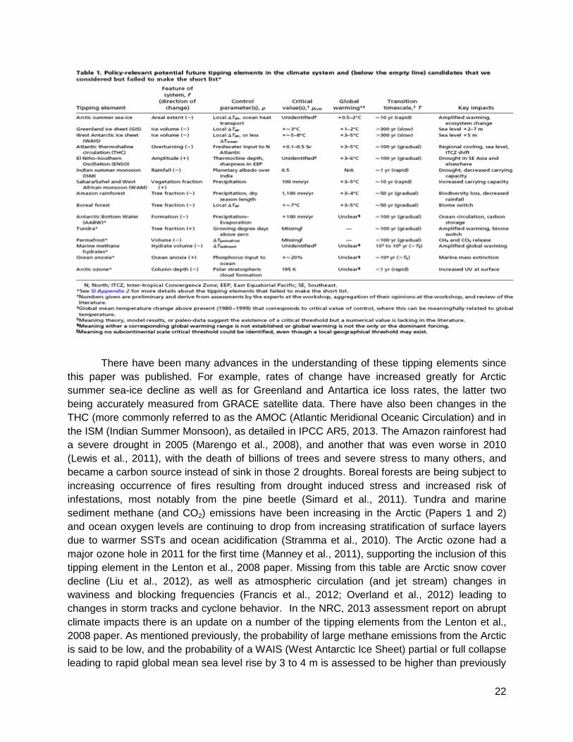
In a review paper by Lenton et al., 2008 the tipping elements in the climate system were
examined. A more recent review of the many tipping point elements located in the Arctic region
is summarized by Duarte et al., 2012. These include Arctic sea ice, terrestrial snow cover,
Greenland ice sheet, North Atlantic deep-water formation regions (for AMOC cycle), boreal
forests, terrestrial permafrost, and marine permafrost and methane hydrates. This Lenton
review paper used a panel of “climate experts” to assess risks of occurrence and resulting
effects of occurrence for various magnitude tipping events and assessed risks and timescales of
the possible occurrences. Table 1 summarizes their basic scope and determinations.
22
There have been many advances in the understanding of these tipping elements since
this paper was published. For example, rates of change have increased greatly for Arctic
summer sea-ice decline as well as for Greenland and Antartica ice loss rates, the latter two
being accurately measured from GRACE satellite data. There have also been changes in the
THC (more commonly referred to as the AMOC (Atlantic Meridional Oceanic Circulation) and in
the ISM (Indian Summer Monsoon), as detailed in IPCC AR5, 2013. The Amazon rainforest had
a severe drought in 2005 (Marengo et al., 2008), and another that was even worse in 2010
(Lewis et al., 2011), with the death of billions of trees and severe stress to many others, and
became a carbon source instead of sink in those 2 droughts. Boreal forests are being subject to
increasing occurrence of fires resulting from drought induced stress and increased risk of
infestations, most notably from the pine beetle (Simard et al., 2011). Tundra and marine
sediment methane (and CO2) emissions have been increasing in the Arctic (Papers 1 and 2)
and ocean oxygen levels are continuing to drop from increasing stratification of surface layers
due to warmer SSTs and ocean acidification (Stramma et al., 2010). The Arctic ozone had a
major ozone hole in 2011 for the first time (Manney et al., 2011), supporting the inclusion of this
tipping element in the Lenton et al., 2008 paper. Missing from this table are Arctic snow cover
decline (Liu et al., 2012), as well as atmospheric circulation (and jet stream) changes in
waviness and blocking frequencies (Francis et al., 2012; Overland et al., 2012) leading to
changes in storm tracks and cyclone behavior. In the NRC, 2013 assessment report on abrupt
climate impacts there is an update on a number of the tipping elements from the Lenton et al.,
2008 paper. As mentioned previously, the probability of large methane emissions from the Arctic
is said to be low, and the probability of a WAIS (West Antarctic Ice Sheet) partial or full collapse
leading to rapid global mean sea level rise by 3 to 4 m is assessed to be higher than previously
23
thought. While there have been significant increases in knowledge on the individual elements
since the 2008 study, there has been little connection between elements or reassessment of
how close they may be to tipping points, and how susceptible they may be to cascading effects
should one element pass a tipping threshold.
The element at highest risk of tipping is most certainly Arctic sea ice; the PIOMAS
volume extrapolation trends to zero ice at the end of the melt season before the end of this
decade. Next at risk may be the Amazon rainforest tipping over in a rapid transition from
rainforest into savannah or shrublands via extreme drought and subsequent massive fire
destruction. Greenland is another very important high-risk tipping element of the system with
water storage in on-land glaciers having the capacity to raise global sea levels 7 meters. With
Arctic sea ice strongly declining, a cascading effect can greatly increase the risk of Greenland
calving acceleration and collapse. Another weak point is the West Antarctic Ice Sheet which is
melting from below by increasing ocean water temperatures. Ocean acidity is another, having
increased by 30 % to 40 % in the last few decades.
Global summary
In summary, there are many signs that we are presently undergoing an abrupt climate
change, at least for some elements of the climate system like the Arctic region. Greenhouse gas
levels have gone up enough to melt significant areas of the Arctic sea ice and snow cover and
greatly reduce the albedo there enough to cause significant Arctic amplification of temperatures
compared to the global mean temperature rise. This in turn has reduced the equator-to-north-
pole temperature gradient reducing the amount of heat transport northward from the equator in
the atmospheric circulation and ocean circulation patterns. This then leads to a slower and
wavier jet stream, and combined with the elevated water vapor content of the atmosphere is
leading to extreme weather events, most notably to torrential downpours and persistant regional
droughts (i.e. California, New Zealand, Australia). The Arctic amplification is also leading to
increasing amounts of methane emissions in the north, contributing to rising global methane
levels and higher regional forcing in the Arctic further amplifying the warming. As the albedo
continues to decrease in the next few years, it is expected that the frequency, intensity,
duration, and spatial extent of the extreme weather events will continue to increase, with
subsequent threats to human well being, the global food supply, and infrastructure, causing
great economic hardship. System stability can no longer be taken for granted.
The key point is that Global Circulation Models (GCMs) for climate that are incorporated
into the IPCC studies do not account properly for the rapid decrease in Arctic albedo (from sea
ice and snow cover declines and Greenland darkening) and subsequent increase in Arctic
temperature amplification, the decreased latitudinal temperature gradient, and the increased
fracturing and waviness of the jet streams causing more extreme weather events. These models
also assume that methane emissions to the atmosphere will not rise significantly this century.
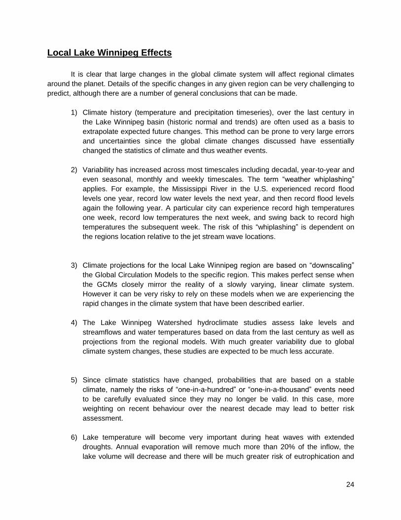
24
Local Lake Winnipeg Effects
It is clear that large changes in the global climate system will affect regional climates
around the planet. Details of the specific changes in any given region can be very challenging to
predict, although there are a number of general conclusions that can be made.
1) Climate history (temperature and precipitation timeseries), over the last century in
the Lake Winnipeg basin (historic normal and trends) are often used as a basis to
extrapolate expected future changes. This method can be prone to very large errors
and uncertainties since the global climate changes discussed have essentially
changed the statistics of climate and thus weather events.
2) Variability has increased across most timescales including decadal, year-to-year and
even seasonal, monthly and weekly timescales. The term “weather whiplashing”
applies. For example, the Mississippi River in the U.S. experienced record flood
levels one year, record low water levels the next year, and then record flood levels
again the following year. A particular city can experience record high temperatures
one week, record low temperatures the next week, and swing back to record high
temperatures the subsequent week. The risk of this “whiplashing” is dependent on
the regions location relative to the jet stream wave locations.
3) Climate projections for the local Lake Winnipeg region are based on “downscaling”
the Global Circulation Models to the specific region. This makes perfect sense when
the GCMs closely mirror the reality of a slowly varying, linear climate system.
However it can be very risky to rely on these models when we are experiencing the
rapid changes in the climate system that have been described earlier.
4) The Lake Winnipeg Watershed hydroclimate studies assess lake levels and
streamflows and water temperatures based on data from the last century as well as
projections from the regional models. With much greater variability due to global
climate system changes, these studies are expected to be much less accurate.
5) Since climate statistics have changed, probabilities that are based on a stable
climate, namely the risks of “one-in-a-hundred” or “one-in-a-thousand” events need
to be carefully evaluated since they may no longer be valid. In this case, more
weighting on recent behaviour over the nearest decade may lead to better risk
assessment.
6) Lake temperature will become very important during heat waves with extended
droughts. Annual evaporation will remove much more than 20% of the inflow, the
lake volume will decrease and there will be much greater risk of eutrophication and
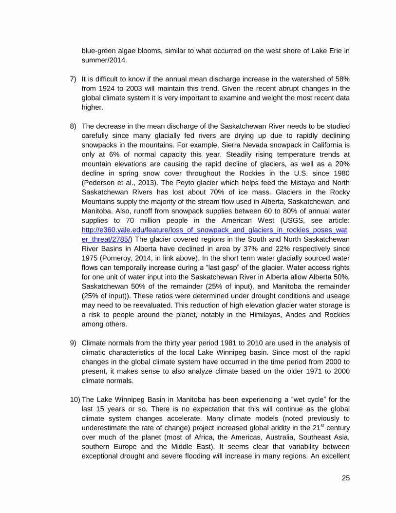
25
blue-green algae blooms, similar to what occurred on the west shore of Lake Erie in
summer/2014.
7) It is difficult to know if the annual mean discharge increase in the watershed of 58%
from 1924 to 2003 will maintain this trend. Given the recent abrupt changes in the
global climate system it is very important to examine and weight the most recent data
higher.
8) The decrease in the mean discharge of the Saskatchewan River needs to be studied
carefully since many glacially fed rivers are drying up due to rapidly declining
snowpacks in the mountains. For example, Sierra Nevada snowpack in California is
only at 6% of normal capacity this year. Steadily rising temperature trends at
mountain elevations are causing the rapid decline of glaciers, as well as a 20%
decline in spring snow cover throughout the Rockies in the U.S. since 1980
(Pederson et al., 2013). The Peyto glacier which helps feed the Mistaya and North
Saskatchewan Rivers has lost about 70% of ice mass. Glaciers in the Rocky
Mountains supply the majority of the stream flow used in Alberta, Saskatchewan, and
Manitoba. Also, runoff from snowpack supplies between 60 to 80% of annual water
supplies to 70 million people in the American West (USGS, see article:
http://e360.yale.edu/feature/loss_of_snowpack_and_glaciers_in_rockies_poses_wat
er_threat/2785/) The glacier covered regions in the South and North Saskatchewan
River Basins in Alberta have declined in area by 37% and 22% respectively since
1975 (Pomeroy, 2014, in link above). In the short term water glacially sourced water
flows can temporaily increase during a “last gasp” of the glacier. Water access rights
for one unit of water input into the Saskatchewan River in Alberta allow Alberta 50%,
Saskatchewan 50% of the remainder (25% of input), and Manitoba the remainder
(25% of input)). These ratios were determined under drought conditions and useage
may need to be reevaluated. This reduction of high elevation glacier water storage is
a risk to people around the planet, notably in the Himilayas, Andes and Rockies
among others.
9) Climate normals from the thirty year period 1981 to 2010 are used in the analysis of
climatic characteristics of the local Lake Winnipeg basin. Since most of the rapid
changes in the global climate system have occurred in the time period from 2000 to
present, it makes sense to also analyze climate based on the older 1971 to 2000
climate normals.
10) The Lake Winnipeg Basin in Manitoba has been experiencing a “wet cycle” for the
last 15 years or so. There is no expectation that this will continue as the global
climate system changes accelerate. Many climate models (noted previously to
underestimate the rate of change) project increased global aridity in the 21st century
over much of the planet (most of Africa, the Americas, Australia, Southeast Asia,
southern Europe and the Middle East). It seems clear that variability between
exceptional drought and severe flooding will increase in many regions. An excellent
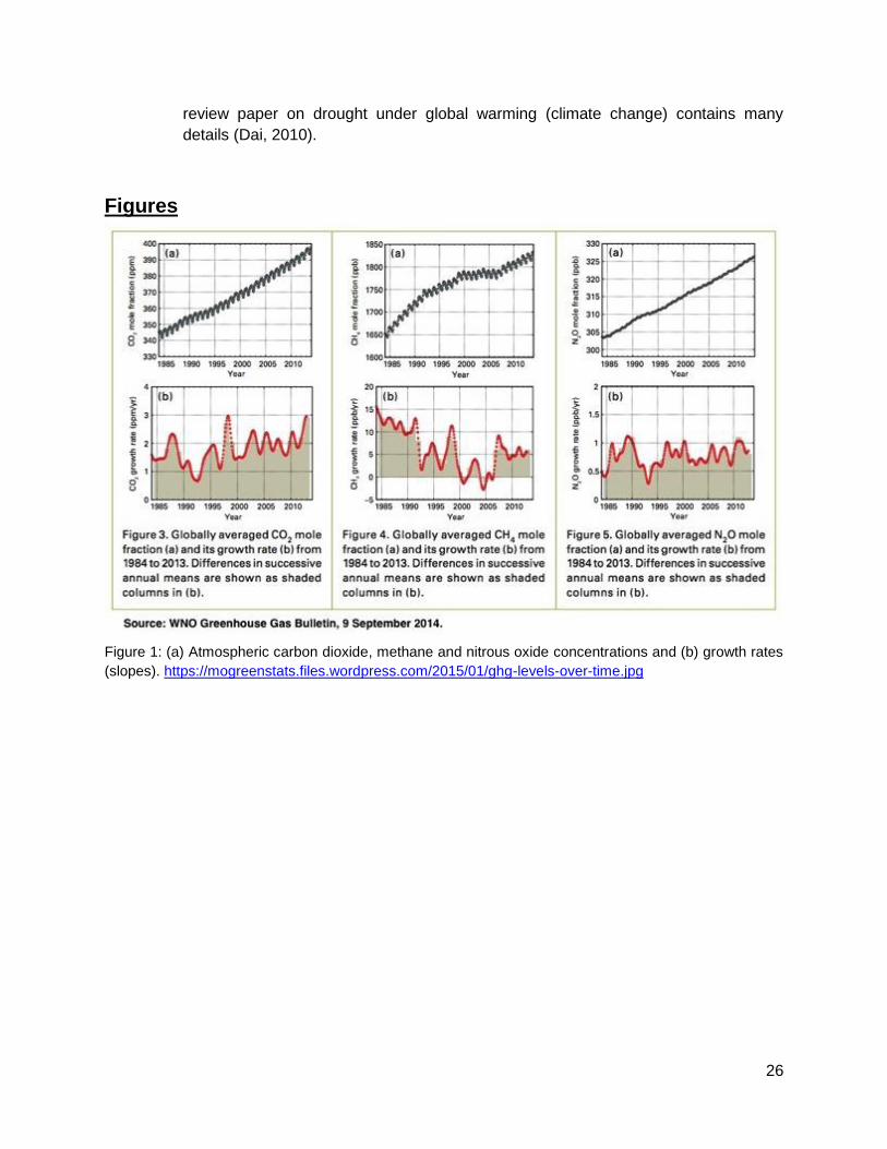
26
review paper on drought under global warming (climate change) contains many
details (Dai, 2010).
Figures
Figure 1: (a) Atmospheric carbon dioxide, methane and nitrous oxide concentrations and (b) growth rates
(slopes). https://mogreenstats.files.wordpress.com/2015/01/ghg-levels-over-time.jpg
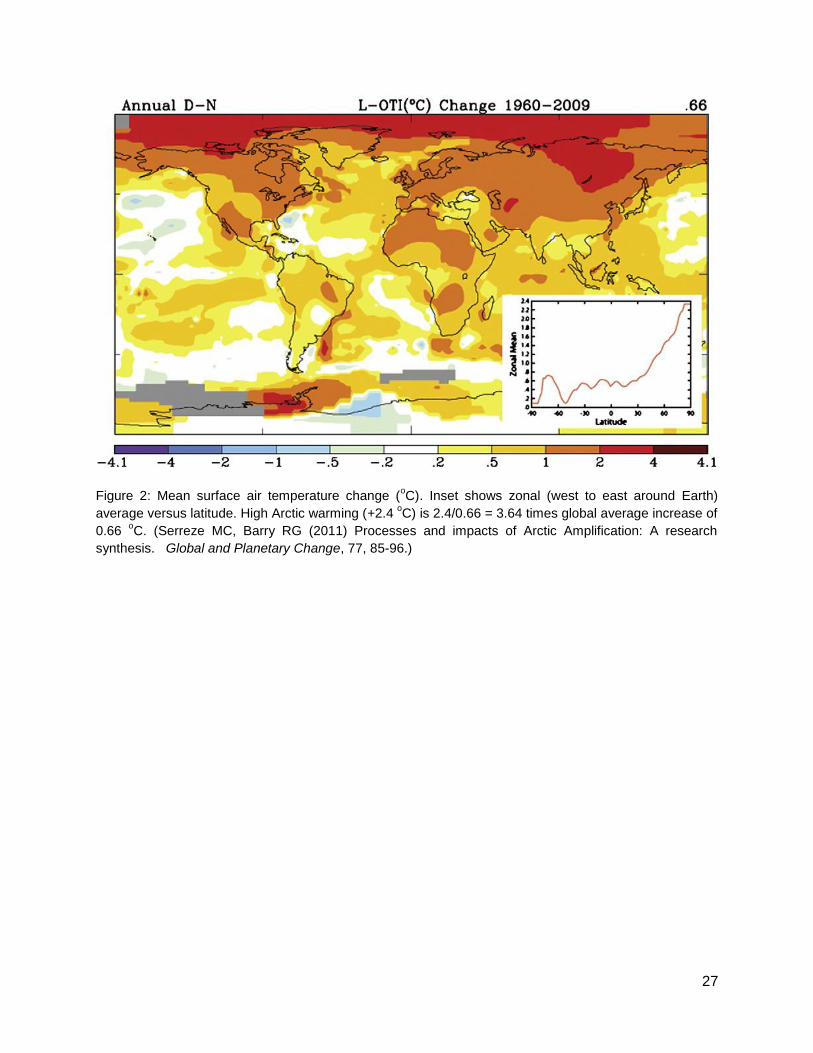
27
Figure 2: Mean surface air temperature change (oC). Inset shows zonal (west to east around Earth)
average versus latitude. High Arctic warming (+2.4 oC) is 2.4/0.66 = 3.64 times global average increase of
0.66 oC. (Serreze MC, Barry RG (2011) Processes and impacts of Arctic Amplification: A research
synthesis. Global and Planetary Change, 77, 85-96.)

28
Figure 3: Seasonal variation of mean surface air temperature change (oC). Inset shows zonal (west to
east around Earth) average versus latitude. High Arctic warming is 6.33x, 2.97x, 2.24x and 5.71x global
average increase for winter, spring, summer and fall, respectively. (Serreze MC, Barry RG (2011)
Processes and impacts of Arctic Amplification: A research synthesis. Global and Planetary Change, 77,
85-96.)
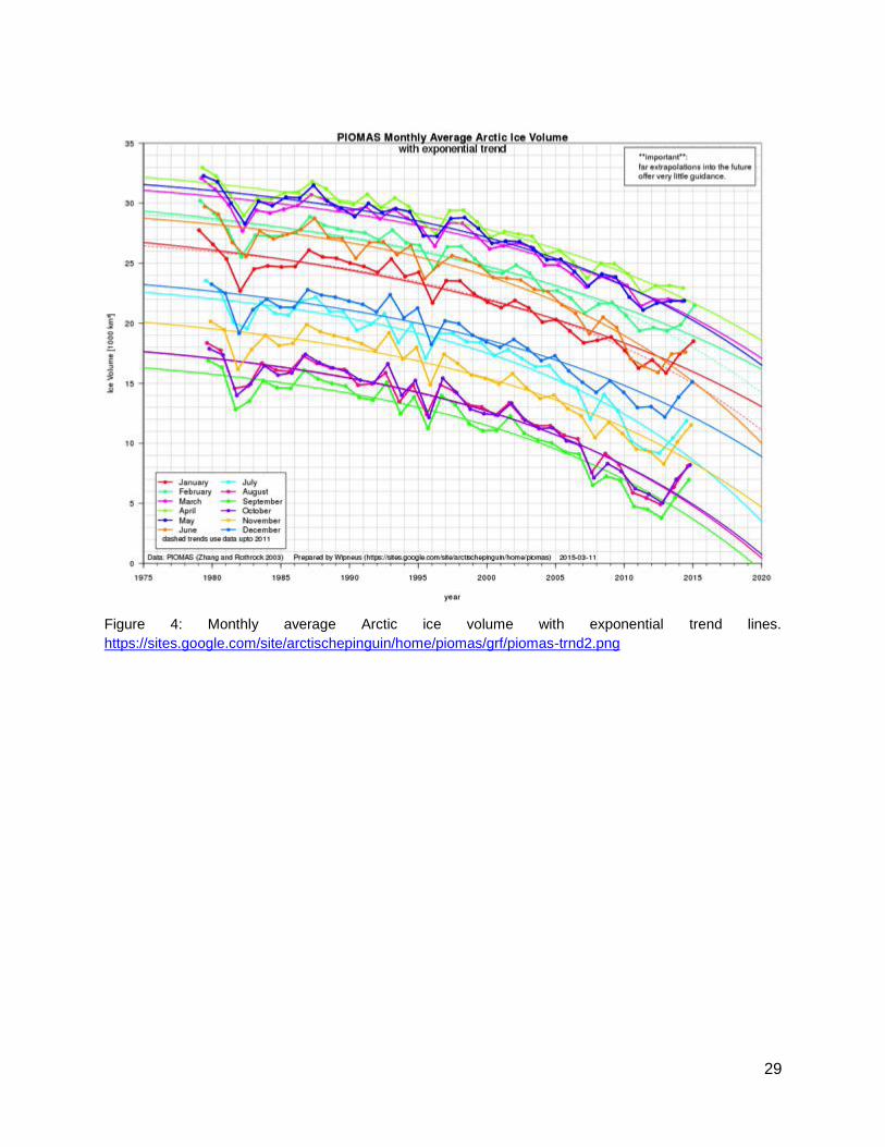
29
Figure 4: Monthly average Arctic ice volume with exponential trend lines.
https://sites.google.com/site/arctischepinguin/home/piomas/grf/piomas-trnd2.png
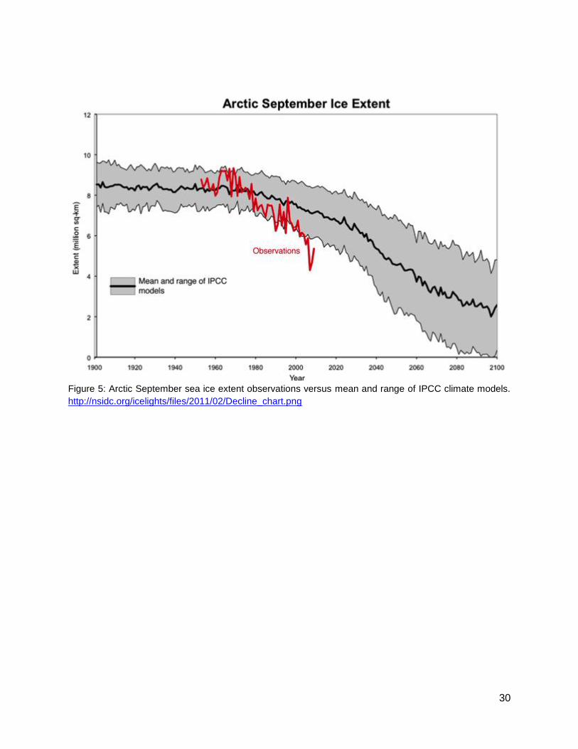
30
Figure 5: Arctic September sea ice extent observations versus mean and range of IPCC climate models.
http://nsidc.org/icelights/files/2011/02/Decline_chart.png
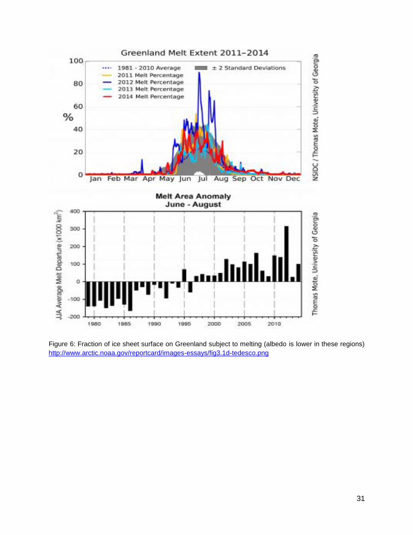
31
Figure 6: Fraction of ice sheet surface on Greenland subject to melting (albedo is lower in these regions)
http://www.arctic.noaa.gov/reportcard/images-essays/fig3.1d-tedesco.png
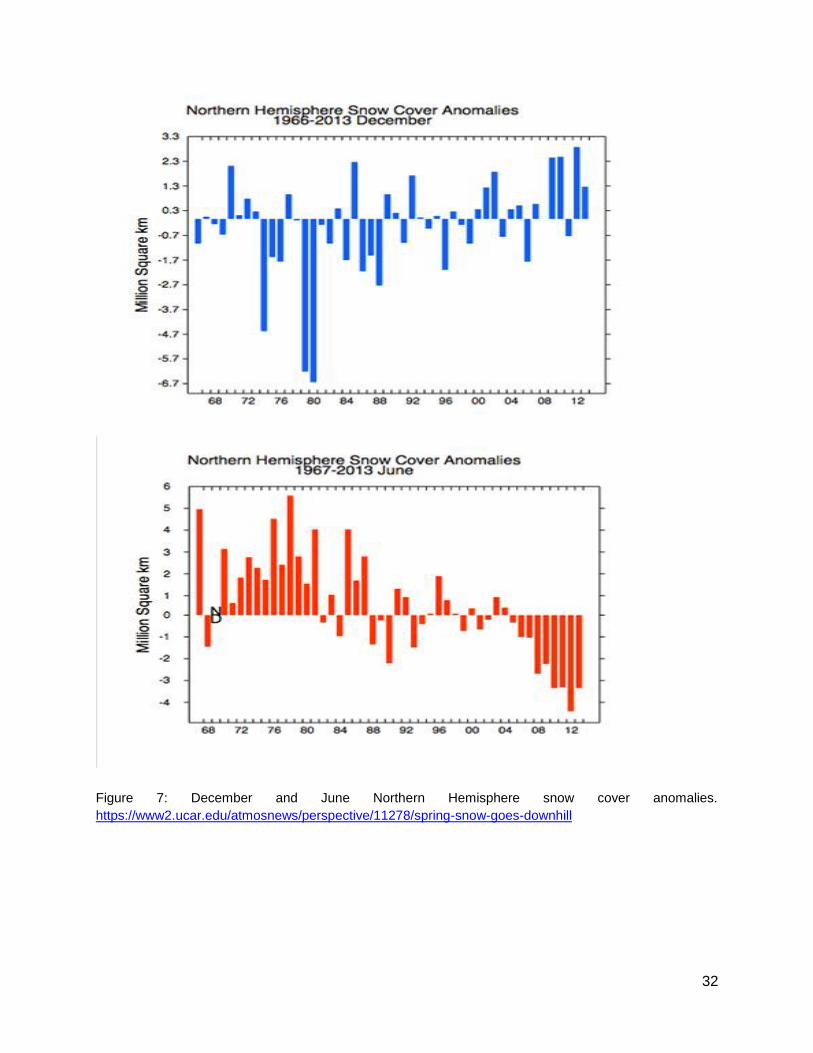
32
Figure 7: December and June Northern Hemisphere snow cover anomalies.
https://www2.ucar.edu/atmosnews/perspective/11278/spring-snow-goes-downhill
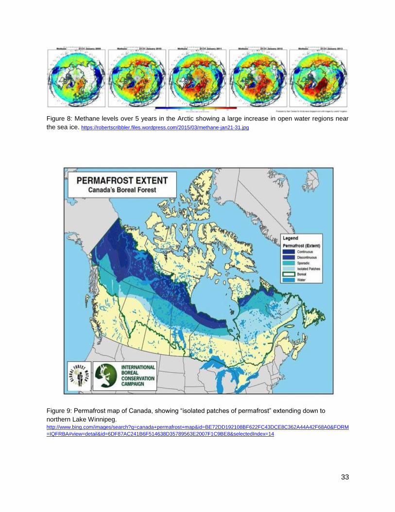
33
Figure 8: Methane levels over 5 years in the Arctic showing a large increase in open water regions near
the sea ice. https://robertscribbler.files.wordpress.com/2015/03/methane-jan21-31.jpg
Figure 9: Permafrost map of Canada, showing “isolated patches of permafrost” extending down to
northern Lake Winnipeg. http://www.bing.com/images/search?q=canada+permafrost+map&id=BE72DD192108BF622FC43DCE8C362A44A42F68A0&FORM
=IQFRBA#view=detail&id=6DF87AC241B6F514638D35789563E2007F1C9BE8&selectedIndex=14
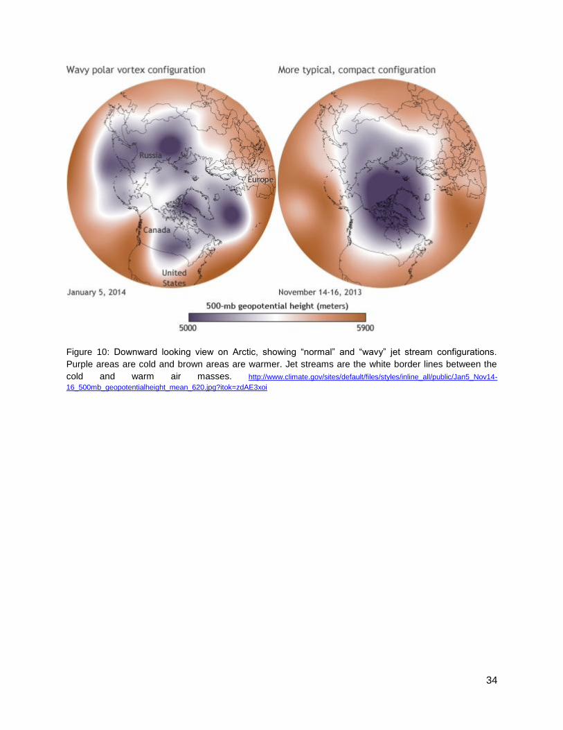
34
Figure 10: Downward looking view on Arctic, showing “normal” and “wavy” jet stream configurations.
Purple areas are cold and brown areas are warmer. Jet streams are the white border lines between the
cold and warm air masses. http://www.climate.gov/sites/default/files/styles/inline_all/public/Jan5_Nov14-
16_500mb_geopotentialheight_mean_620.jpg?itok=zdAE3xoi
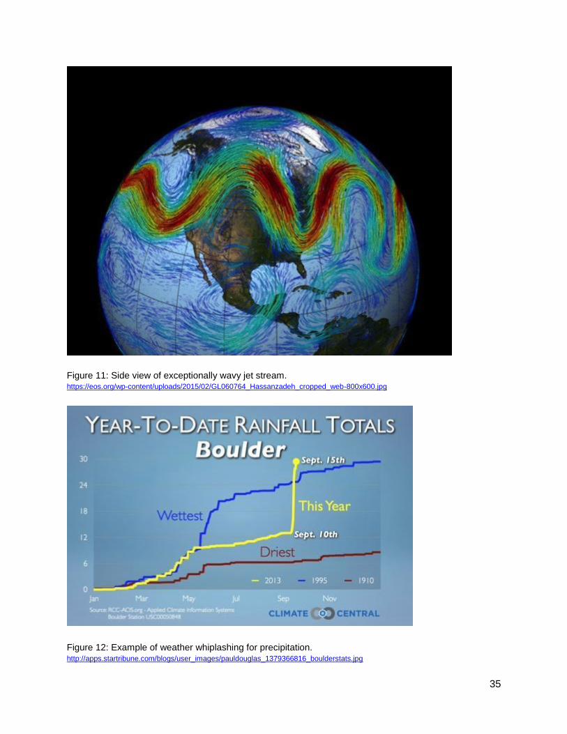
35
Figure 11: Side view of exceptionally wavy jet stream. https://eos.org/wp-content/uploads/2015/02/GL060764_Hassanzadeh_cropped_web-800x600.jpg
Figure 12: Example of weather whiplashing for precipitation. http://apps.startribune.com/blogs/user_images/pauldouglas_1379366816_boulderstats.jpg
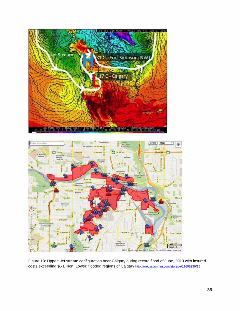
36
Figure 13: Upper: Jet stream configuration near Calgary during record flood of June, 2013 with insured
costs exceeding $6 Billion; Lower: flooded regions of Calgary http://media.twnmm.com/storage/11698939/15
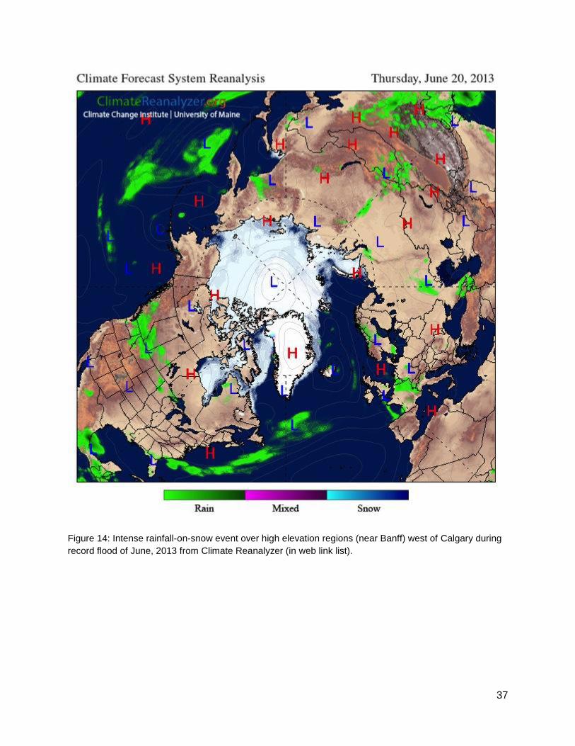
37
Figure 14: Intense rainfall-on-snow event over high elevation regions (near Banff) west of Calgary during
record flood of June, 2013 from Climate Reanalyzer (in web link list).
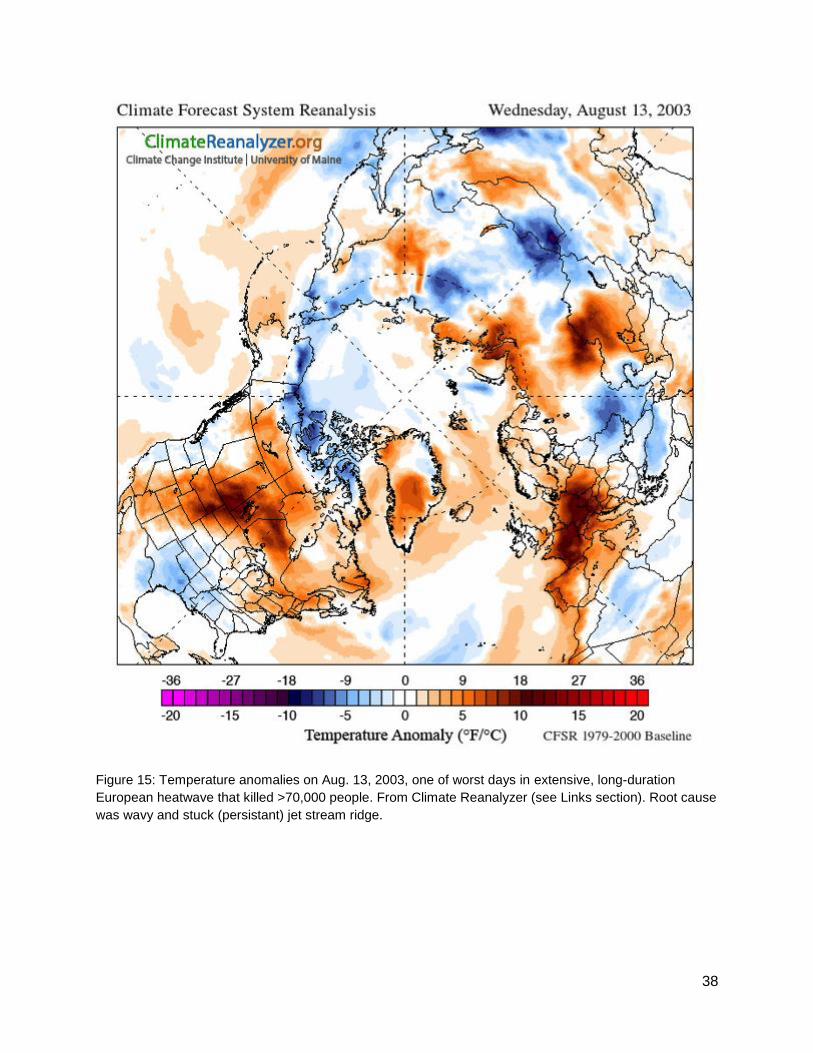
38
Figure 15: Temperature anomalies on Aug. 13, 2003, one of worst days in extensive, long-duration
European heatwave that killed >70,000 people. From Climate Reanalyzer (see Links section). Root cause
was wavy and stuck (persistant) jet stream ridge.
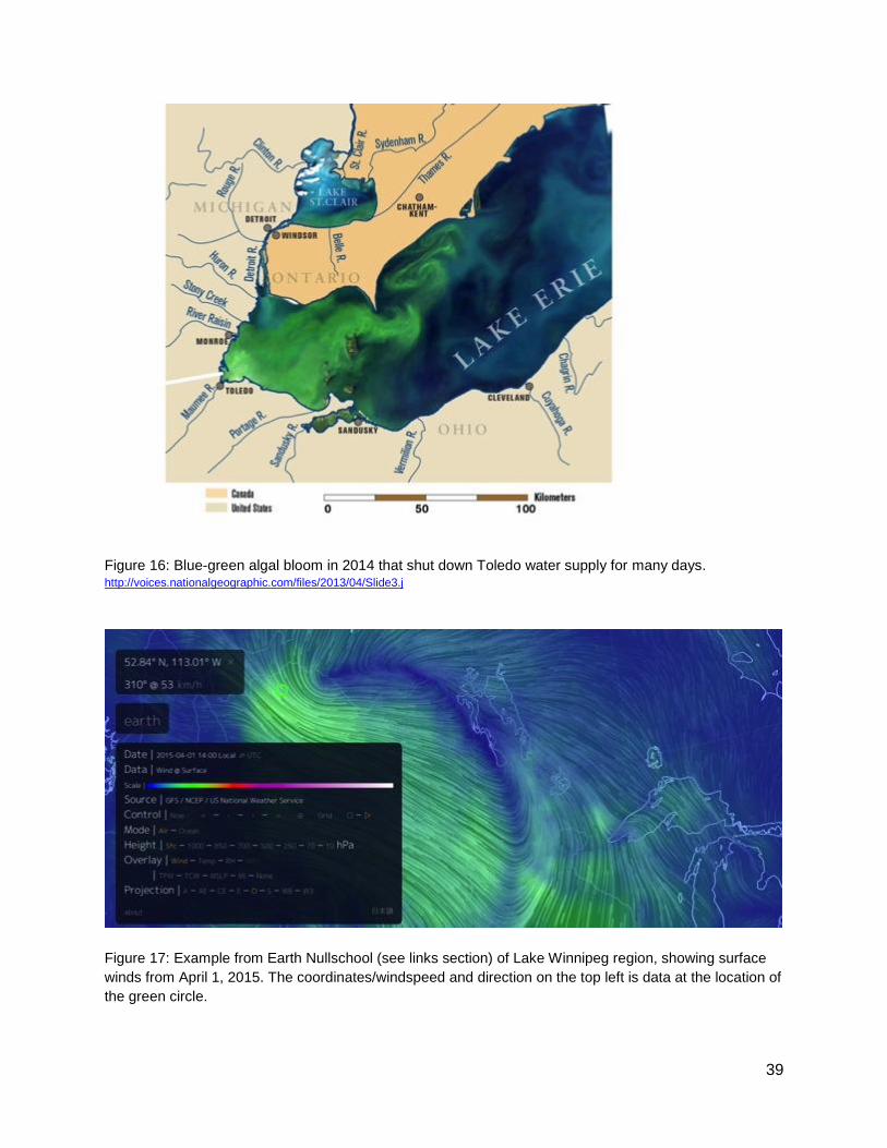
39
Figure 16: Blue-green algal bloom in 2014 that shut down Toledo water supply for many days. http://voices.nationalgeographic.com/files/2013/04/Slide3.j
Figure 17: Example from Earth Nullschool (see links section) of Lake Winnipeg region, showing surface
winds from April 1, 2015. The coordinates/windspeed and direction on the top left is data at the location of
the green circle.
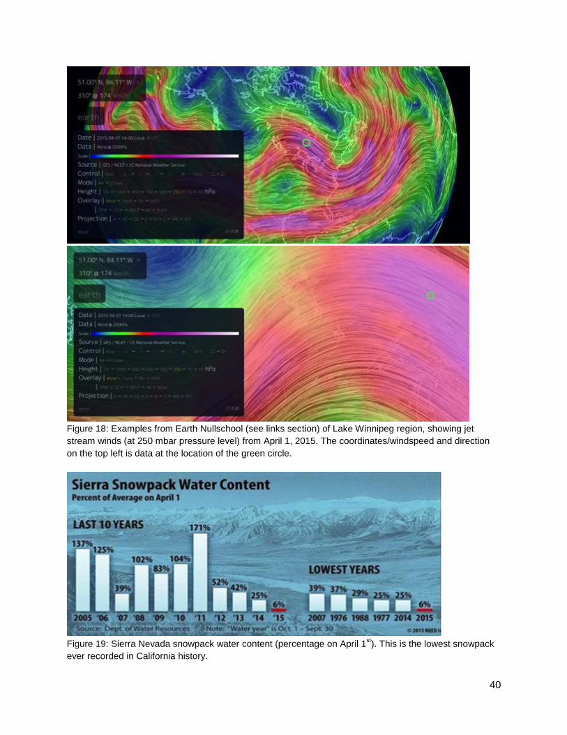
40
Figure 18: Examples from Earth Nullschool (see links section) of Lake Winnipeg region, showing jet
stream winds (at 250 mbar pressure level) from April 1, 2015. The coordinates/windspeed and direction
on the top left is data at the location of the green circle.
Figure 19: Sierra Nevada snowpack water content (percentage on April 1
st). This is the lowest snowpack
ever recorded in California history.
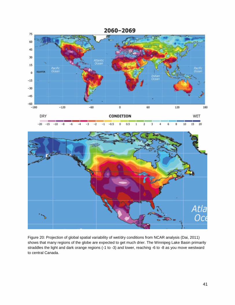
41
Figure 20: Projection of global spatial variability of wet/dry conditions from NCAR analysis (Dai, 2011)
shows that many regions of the globe are expected to get much drier. The Winnipeg Lake Basin primarily
straddles the light and dark orange regions (-1 to -3) and lower, reaching -6 to -8 as you move westward
to central Canada.
42
Glossary
Abrupt climate change: nonlinear (such as exponential, versus a linear (straight line) increase;
extremely rapid rates of change, tipping point, threshold passed and a change in state occurs.
Good examples of abrupt processes are freezing, thawing, snapping a stick, tipping a canoe…
Albedo: Reflectivity of a surface, lower numbers darker, higher numbers whiter, average albedo
of Earth from space is about 30%, albedo of fresh snow is about 90%, older snow and ice about
80 to 90%, dark sea water about 10%, forests about 30%. Arctic region albedo has declined
from about 54% to 48% over 3 decades
Anthropogenic: Human caused/influenced
Climate system: Includes the elements of atmosphere, lithosphere, cryosphere, hydrosphere,
biosphere, and also the external forcings (sun, volcanos which are really part of lithosphere)
Feedback: After applying a forcing to a system there is a response proportional to the forcing
(linear regime). If the response causes the forcing to increase it is called a positive or reinforcing
feedback, and if the response reduces the forcing it is a negative or braking feedback. Warming
in the Arctic reduces the albedo. This darkens the surfaces, and results in more solar radiation
absorbed and thus even more warming and even more albedo reduction (positive feedback).
Glaciers: Describes ice on mountain tops, and also ice caps. Glaciers flow downhill, and on
Greenland and Antarctica they extend off the coasts to create Ice Shelves. Large calving events
on the ice shelves create iceburgs.
Ice caps: Ice that sits on bedrock, such as on Greenland and Antarctica. This ice can be
grounded on bedrock that is located far below sea level, and in this case is vulnerable to warm
ocean water melting from below.
IPCC: Intergovernmental Panel on Climate Change, a group under UNFCCC (United Nations
Framework Convention on Climate Change) that publishes climate change reviews every 5 to 7
years on a)Physical Science Basis, b) Adaptation, and c)Mitigation. AR5 (Assessment Report 5)
is the 5th iteration of the report.
Jet streams: High altitude winds (at tropopause, which seperates lower atmosphere
(troposphere) from higher atmosphere (stratosphere); they also at high latitudes and circle the
globe primarily zonally (from west to east) with meridional waves (north to south and south to
north components). Separate cold fronts (such as cold and dry Arctic air) from warm fronts
(such as warm and moist air from the equator). Guide storms, wavier jet streams cause large
pressure differences and thus increase frequency, severity and duration of extreme weather
events.
43
Methane hydrates: An ice lattice that surrounds a methane molecule. When the lattice melts
the volume expands by about 169 times and the methane is released. Exist at a combination of
low pressures and high pressures, such as those that exist at ocean pressures at 200 meters
(shallower in ocean sediments). Also located in permafrost regions.
Proxies: Indirect measurements of climate (temperature, precipitation) from marine sediment
coring, ice cores, coral growth, tree rings for example. The instrumental record is the direct
measurement of climate over the past century or so.
Rossby waves: Refers to the waviness in the jet streams as they circle the Earth at high
latitudes and high altitudes.
Sea ice: Ice that forms over the ocean in winters, and melts back in summers. In the Arctic
average sea ice thickness has exponentially declined over last 30 years. Sea ice extent is
defined as the area over which the ice concentration is equal to or greater than 15% ice. Sea ice
area is defined as the area over which the ice concentration is 100% (polynyas are regions
within that are open water). Sea ice area and extent are easily measured with satellite sensors,
sea ice thickness is measured from satellite via freeboard (thickness of ice above water surface)
by precise radar altimetry. Sea ice volume is calculated from area and thickness.
Key web links
Arctic sea ice graphs: Real-time time series plots on sea ice extent, area, thickness, motion;
maps on ice locations, meteorology, ocean temperatures and conditions, ocean buoy data, all
updated daily: https://sites.google.com/site/arcticseaicegraphs/
Climate Reanalyzer: Real-time information on atmospheric weather and ocean conditions, displayed in a
different format to Earth nullschool; great for examining global temperature anomalies (difference
between present day and climate normal): http://www.cci-reanalyzer.org/
Earth nullschool: Real-time Earth sphere projections for atmospheric weather (temperatures,
precipitation, winds at pressure levels up to top of troposphere (lower atmosphere where
weather occurs); also data on oceans (temperatures, currents, etc.); click on text “earth” in
bottom left corner to access variables, drag to rotate view, use slider to zoom, click on location
for local (point) measurement: http://earth.nullschool.net/
Lima, Peru COP20 presentation that I gave at a press conference on the present state of the climate
system: https://www.youtube.com/watch?v=QQkNxuQ0DoI
Climate system disruption video that I created March 24, 2015:
https://www.youtube.com/watch?v=GR2RDwhBFh4
Many other climate system videos on my YouTube channel, linked on Twitter and Facebook
44
References
Alley RB, Marotzke J, Nordhaus WD, Overpeck JT, Peteet DM, Pielke Jr RA, Pierrehumbert RT, Rhines PB,
Stocker TF, Talley LD, Wallace JM (2003) Abrupt climate change. Science, 299, 2005-2010.
ACIA (2004) Impacts of a warming Arctic: synthesis report of the Arctic climate impact assessment. Fairbanks, Alaska: Arctic Climate Impact Assessment. http://www.acia.uaf.edu/pages/overview.html
AIRS (Atmospheric Infrared Sounder) satellite data, NCAR/UCAR, https://climatedataguide.ucar.edu/climate-
data/airs-atmospheric-infrared-sounder-version-6-level-2
AMAP, 2009 (Arctic Monitoring and Assessment Program) AMAP 2009 update on selected climate issues of
concern (observations, short-lived climate forcers, Arctic carbon cycle, predictive capability). Oslo, Norway.
AMAP, 2012 (Arctic Monitoring and Assessment Program) Arctic Climate Issues 2011: Changes in Arctic
snow, water, ice and permafrost in the Arctic. SWIPA 2011 (Snow, Water, Ice and Permafrost in the Arctic)
overview report, Oslo, Norway.
Archer D (2010) The global carbon cycle. Princeton University Press: Princeton, NJ, 205p.
BAMS (2012) State of the climate in 2011. Special supplement to the Bulletin of the American Meteorological
Society, 93(7), July, 264p.
BAMS (2013) State of the climate in 2012. Special supplement to the Bulletin of the American Meteorological
Society.
Barnes EA (2013) Revisiting the evidence linking Arctic amplification to extreme weather in midlatitudes.
Geophysical Research Letters, 40, 6p.
Barnosky AD, Matzke N, Tomiya S, Wogan GOU, Swartz B, Quental TB, Marshall C, McGuire JL, Lindsey EL,
Maguire KC, Mersey B, Ferrer EA (2011) Has the Earth’s sixth mass extinction already arrived? Nature 471,
51-57.
Barnosky AD, Hadly EA, Bascompte J, Berlow EL, Brown JH, Fortelius M, Getz WM, Harte J, Hastings A,
Marquet PA, Martinez ND, Mooers A, Roopnarine P, Vermeij G, Williams JW, Gillespie R, Kitzes J, Marshall C,
Matzke N, Mindell DP, Revilla E, Smith AB (2012) Approaching a state shift in Earth’s biosphere. Nature 486,
52-58.
Barry RG, Carleton AM. 2001. Synoptic and dynamic climatology. Routledge, London, UK, 620p.
Barry RG, Chorley RJ (2010) Atmosphere, Weather and Climate (9th Edition). Routledge, New York, 516p.
Beaulieu C, Chen, J, Sarmiento JL, 2012. Change-point analysis as a tool to detect abrupt climate variations.
Phil. Trans. R. Soc. A., March 13, 370(1962), 1228-1249.
45
Beckwith P (2012) (unpublished) Our climate system. Blog (The Canadian Daily),
http://www.thecanadiandaily.ca/2012/12/05/paul-beckwith-our-climate-system/
Beckwith P (2012b) (unpublished) A possible link between Hurricane Sandy on the east coast and seismic
activity on the west coast. Gazette publication, University of Ottawa,
http://www.gazette.uottawa.ca/en/2012/11/a-possible-link-between-hurricane-sandy-on-the-east-coast-and-
seismic-activity-on-the-west-coast/
Betts RA, Collins M, Hemming DL, Jones CD, Lowe JA, Sanderson MG (2011) When could global warming
reach 4 oC? Philosophical Transactions of the Royal Society A, 369(1934), 67-84.
Box JE, Cappelen J, Chen C, Decker D, Fettweis X, Mote T, Tedesco M, van de Val RSW, Wahr J (2013)
Arctic Report Card : Update for 2012. http://www.arctic.noaa.gov/reportcard/greenland_ice_sheet.html
Box, JE, Fettweis X, Stroeve JC, Tedesco M, Hall DK, Steffen K (2012) Greenland ice sheet albedo feedback:
thermodynamics and atmospheric drivers. The Cryosphere, 6, 821-839.
Bridgeman HA, Oliver JE (2006) The Global Climate System, Patterns, Processes, and Teleconnections.
Cambridge University Press, Cambridge, UK, 331p.
Broecker W (2010) The Great Ocean Conveyer: Discovering the trigger for abrupt climate change. Princeton
University Press, Princeton, US, 154p.
Brothers LL, Van Dover CL, German CR, Kaiser CL, Yoerger DR, Ruppel CD, Lobeckwer E, Skarke AD,
Wagner JKS (2013) Evidence for extensive methane venting on the southeastern U.S. Atlantic margin.
Geology, G34217.1
Bruhwiler L, Dlugokencky E (2012) Carbon dioxide (CO2) and methane (CH4). Arctic Report Card: Update for
2012. Boulder, CO, USA: NOAA Earth System Research Laboratory (ESRL) Global Monitoring Division.
Carlson AE, Winsor K (2012) Northern hemisphere ice-sheet responses to past climate warming. Nature
Geoscience, 5, 607-612.
Carter P (2013) The compelling case in climate change science for an emergency upgrading of Arctic
monitoring capacities. (unpublished correspondence).
Ceres (2013) Guide for responsible corporate engagement in climate policy.
http://www.ceres.org/resources/reports/guide-for-responsible-corporate-engagement-in-climate-policy/view
Chapman Conference on Abrupt Climate Change: Conference proceedings. (2009) Byrd Polar Research
Center, Ohio State University, June 15-17.
Cimatoribus AA, Drijfhout SS, Livina V, van der Schrier G (2012) Dansgaard-Oeschger events: tipping points in
the climate system. Clim. Past Discuss., 8, 4269-4294.
Comiso, JC (2012) Large Decadal Decline of the Arctic Multiyear Ice Cover. J. Climate, 25, 1176–1193.
46
Cornell SE, Prentice IC, House JI, Downy CJ. 2012. Understanding the Earth System: Global change science
for application. Cambridge University Press, Cambridge, UK, 267p.
Coumou D, Rahmstorf S (2012) A decade of weather extremes. Nature Climate Change, 2, 491-496.
Crawley MJ (2013) The R Book. John Wiley & Sons, Ltd. United Kingdom, 1051p.
Cronin TM (2009) Paleoclimates: Understanding Climate Change Past and Present. Columbia University
Press, New York, 448p.
Crutzen PJ, Steffen W (2003) How Long Have We Been in the Anthropocene Era? Climatic Change, 61(3)
251-257.
Dai A (2011) Drought under global warming: a review Wires.wiley.com/climatechange, 2(January/February),
http://onlinelibrary.wiley.com/doi/10.1002/wcc.81/epdf
Dakos V, Scheffer M, van Nes EH, Brovkin V, Petoukhov V, Held H. 2008. Slowing down as an early warning
signal for abrupt climate change. PNAS, Sept. 23, 105(38), 14308-14312.
Davidson EA, de Araujo AC, Artaxo P, Balch JK, Brown IF, Bustamante MMC, Coe MT, DeFries RS, Keller M,
Longo M, Munger JW, Schroeder W, Soares-Filho BS, Souza Jr CM, Wofsy SC (2012) The Amazon basin in
transition. Nature, 481, 321-328.
Davy B, Pecher I, Wood R, Carter L, Gohl K (2010) Gas escape features off New Zealand: Evidence of
massive release of methane from hydrates. Geophysical Research Letters, 37, L21309, 5p.
DeConto RM, Galeotti S, Pagani M, Tracy D, Schaefer K, Zhang T, Pollard D, Beerling DJ (2012) Past extreme
warming events linked to massive carbon release from thawing permafrost. Nature, 484, 87-91.
Derksen C, Brown R (2012a) Spring snow cover extent reductions in the 2008-2012 period exceeding climate
model projections. Geophysical Research Letters, 39 (19), L19504, 6p.
Derksen C, Brown R (2012b) Snow. Arctic Report Card: Update for 2012, NOAA,
http://www.arctic.noaa.gov/reportcard/snow.html
Deschamps P, Durand N, Bard E, Hamelin B, Camoin G, Thomas AL, Henderson GM, Okuno J, Yokoyama Y
(2012) Ice-sheet collapse and sea-level rise at the Bolling warming 14,600 years ago. Nature, 483(7391), 559-
564.
Dettinger M (2011) Climate change, atmospheric rivers, and floods in California – A multimodel analysis of
storm frequency and magnitude changes. Journal of the American Water Resources Association (JAWRA),
47(3), 514-523.
Dettinger M, Ingram BL (2013) The coming megafloods. Scientific American 308, 64 – 71.
Dlugokencky EJ, Nisbet EG, Fisher R, Lowry D (2011) Global atmospheric methane: budget, changes, and
dangers. Philosophical Transactions of the Royal Society A, 369(1943), 2058-2072.
47
Doha Climate Change conference report (2012). Earth Negotiations Bulletin, UN COP18,
http://www.iisd.ca/download/pdf/enb12567e.pdf
Duarte CM, Lenton TM, Wadhams P, Wassmann P (2012) Abrupt climate change in the Arctic. Nature Climate
Change, 2, 60-62.
Dyck S, Tremblay LB, de Vernal A (2010) Arctic sea-ice cover from the early Holocene : the role of
atmospheric circulation patterns. Quaternary Science Reviews, 29, 3457-3467.
Elberling B, Christiansen HH, Hansen BU (2010) High nitrous oxide production from thawing permafrost.
Nature Geoscience 3, 332-335.
Ehrlich PR, Ehrlich AH. Can a collapse of global civilization be avoided? 2013. Proc. R. Soc. B, 280,
20122845, Jan 9.
ESRL (Earth System Research Laboratory) Global Monitoring Division,
http://www.esrl.noaa.gov/gmd/obop/mlo/programs/esrl/methane/methane.html;
http://www.esrl.noaa.gov/gmd/dv/iadv/
Fisher RE, Sriskantharajah S, Lowry D, Lanoiselle M, Fowler CMR, James RH, Hermansen O, Lund-Myhre C,
Stohl A, Greinert J, Nisbet-Jones PBR, Mienert J, Nisbet EG (2011) Arctic methane sources: Isotopic evidence
for atmospheric inputs. Geophysical Review Letters, 38(21).
Flanner MG, Shell KM, Barlage M, Perovich DK, Tschudi MA (2011) Radiative forcing and albedo feedback
from the Northern Hemisphere cryosphere between 1979 and 2008. Nature Geoscience, 4, 151-155.
Francis JA, Vavrus SJ (2012) Evidence linking Arctic amplification to extreme weather in mid-latitudes.
Geophysical Research Letters, 39, LO6801, 6p.
Frieler K, Meinshausen M, Braun N, Golly A, Hare W, Mengel M, van der Merwe K, Poulter B, Schaeffer M,
Schleussner C-F, von Deimling T (2011) Risk-analysis of global climate tipping points. PRIMAP Research
Group, Potsdam Institute for Climate Impact Research.
Fry JL, Graf H-F, Grotjahn R, Raphael MN, Saunders C, Whitaker R (2010) The encyclopedia of weather and
climate change, A complete visual guide. University of California Press, Berkeley, 512p.
Glikson AY (2014) Evolution of the Atmosphere, fire and the Anthropocene climate event horizon. Springer
Briefs in Earth Sciences. http://download.springer.com/static/pdf/843/bok%253A978-94-007-7332-
5.pdf?auth66=1386351867_dba3eb996aeef7be0c3285c05b051b30&ext=.pdf
Gunther F, Overduin PP, Sandakov AP, Grosse G, Grigoriev MN (2013a) Short- and long-term thermo-erosion
of ice-rich permafrost coasts in the Laptev Sea region. Biogeosciences, 10, 4297-4318
Gunther F, Overduin PP, Baranskaya A, Opel T, Grigoriev MN (2013b) Observing Muostakh Island disappear:
erosion of a ground-ice-rich coast in response to summer warming and sea ice reduction on the East Siberian
shelf. The Cryosphere Discuss., 7, 4101-4176.
48
Hansen JE, Sato M, Kharecha P, Russell G, Lea DW, Siddall M (2007) Climate change and trace gases.
Philosophical Transactions of the Royal Society A, 365, 1925-1954.
Hansen JE, Sato M, Kharecha P, Schuckmann K. von (2011) Earth’s energy imbalance and implications.
Atmos. Chem. Phys. 11, 13421-13449.
Hansen J, Sato M, Ruedy R (2012a) Perception of climate change. PNAS, doi: 10.1073/pnas.1205276109
Hansen JE, Sato M (2012b) Climate sensitivity estimated from Earth’s climate history. NASA GISS report, New
York. http://www.columbia.edu/~jeh1/mailings/2012/20120508_ClimateSensitivity.pdf
Hansen J, Kharecha P, Sato M, Masson-Delmotte V, Ackerman F, Beerling DJ, Hearty PJ, Hoegh-Gulberg O,
Hsu S-L, Parmesan C, Rockstrom J, Rohling EJ, Sachs J, Smith P, Steffen K, van Susteren L, von
Schuckmann K, Zachos JC (2013) Assessing “Dangerous climate change”: Required reduction of carbon
emissions to protect young people, future generations and nature. PLOS 1, 8(12), e81648, 26p.
Holmes J, Lowe J, Wolff E, Srokosz M (2011) Rapid climate change: lessons from the recent geological past.
Glob. Planet. Change. doi:10.1016/j.gloplacha.2010.10.005
IASI (Infrared Atmospheric Sounding Interferometer) EUMETSAT (European Meterorological Satellite data), http://www.eumetsat.int/website/home/Satellites/CurrentSatellites/Metop/MetopDesign/IASI/index.html IPCC (FAR, 1991) Climate Change 1991: The Scientific Basis. Contribution of Working Group I to the First Assessment Report of the Intergovernmental Panel on Climate Change. IPCC (SAR, 1996) Climate Change 1996: The Scientific Basis. Contribution of Working Group I to the Second Assessment Report of the Intergovernmental Panel on Climate Change. IPCC (TAR, 2001) Climate Change 2001: The Scientific Basis. Contribution of Working Group I to the Third Assessment Report of the Intergovernmental Panel on Climate Change. Houghton, JT,Ding Y, Griggs DJ, Noguer M, van der Linden PJ, Dai X, Maskell K, Johnson CJ(eds.). Cambridge University Press, Cambridge, United Kingdom and New York, NY, USA, 881pp.
IPCC (AR4, 2007) Climate Change 2007: The Physical Science Basis. Contribution of Working Group I to the Fourth Assessment Report of the Intergovernmental Panel on Climate Change. Solomon S, Qin D, Manning M, Marquis M, Averyt K, Tignor MB, Miller Jr. HL, Chen Z (eds.). Cambridge University Press, Cambridge, United Kingdom and New York, NY, USA. IPCC (AR5, 2013) Working Group I Contribution to the IPCC Fifth Assessment Report Climate Change 2013: The Physical Science Basis, Final Draft Underlying Scientific-Technical Assessment (report accepted by Working Group I of the IPCC but not approved in detail), September 26. IPCC SREX (2012) Managing the risks of extreme events and disasters to advance climate change adaptation, Special Report of the Intergovernmental Panel on Climate Change. (eds) Field CB, Barros V, Stocker TF, Dahe Q, Dokken DJ, Ebi KL, Mastrandrea MD, Mach KJ, Plattner G-K, Allen SK, Tignor M, Midgley PM, Cambridge University Press, Cambridge, United Kingdom and New York, NY, USA. Jaiser R, Dethloff K, Handorf D, Rinke A, Cohen J (2012) Impact of sea ice cover changes on the Northern Hemisphere atmospheric winter circulation. Tellus A, 64, 11p.
49
Kennett, JP, Cannariato KG, Hendy IL, Behl RJ, 2003. Methane Hydrates in Quaternary Climate Change: The
Clathrate Gun Hypothesis, 216 pp., AGU, Washington, D. C., doi:10.1029/054SP.
Kirschke S, Bousquet P, Ciais P, Saunois M, Canadell JG, Dlugokencky EJ, Bergamaschi P, Bergmann D, Blake DR, Bruhwiler L, Cameron-Smith, P, Castaldi S, Chevalier F, Feng L, Fraser, A, Heimann M, Hodson EL, Houweling S, Josse B, Fraser PJ, Krummel PB, Lamarque J-F, Langenfelds RL, Le Quere C, Naik V, O’Doherty S, Palmer PI, Pison I, Plummer D, Poulter B, Prinn RG, Rigby M, Ringeval B, Santini M, Schmidt M, Shindell DT, Simpson IJ, Spahni R, Steele LP, Strode SA, Sudo K, Szopa S, van der Werf GR, Voulgarakis A, van Weele M, Weiss RF, Williams JE, Zeng G (2013) Three decades of global methane sources and sinks. Nature Geoscience, 6, 813-823. Lang C, Leuenberger M, Schwander J, Johnsen S (1999) 16oC rapid temperature variation in central Greenland 70,000 years ago. Science, 286(5441), 934-937.
Laxon SW, Giles KA, Ridout AL, Wingham DJ, Willatt R, Cullen R, Kwok R, Schweiger A, Zhang AJ, Haas C,
Hendricks S, Krishfield R, Kurtz N, Farrell S, Davidson M (2013) CryoSat-2 estimates of Arctic sea ice
thickness and volume. Geophys. Res. Lett., 40, 732–737.
Lenton TM, Held H, Kriegler E, Hall JW, Lucht W, Rahmstorf S, Schellnhuber HJ (2008) Tipping elements in
the Earth’s climate system. PNAS, 105(6), 1786-1793.
Lenton TM, Livina VN, Dakos V, Scheffer M. 2012. Climate bifurcation during the last deglaciation. Clim. Past
Discuss., 8, 321-348.
Lenton TM (2013) Game theory: tipping climate cooperation. Nature Climate Change (News and Views),
doi:10.1038/nclimate2078
Lesins G, Duck TJ, Drummond JR (2012) Surface Energy Balance Framework for Arctic Amplification of
Climate Change. J. Climate, 25, 8277–8288.
Lesins G (2013) Arctic climate change. Presentation at the Create Summer School located in Alliston, July.
http://www.candac.ca/create/ss2013/talks/Day3_Lesins_L3_climate_change.pdf
Levine JG, Wolff EW, Jones AE, Sime LC, Valdes PJ, Archibald AT, Carver GD, Warwick NJ, Pyle JA (2011)
Reconciling the changes in atmospheric methane sources and sinks between the Last Glacial Maximum and
the pre-industrial era. Geophysical Research Letters, 38(23), 6p.
Levine JG, Wolff EW, Hopcroft PO, Vlades PJ (2012) Controls on the tropospheric oxidizing capacity during an
idealized Dansgaard-Oeschger event, and their implications for the rapid rises in atmospheric methane during
the last glacial period. Geophysical Review Letters, 39(12), 7p.
Lewis SL, Brando PM, Phillips OL, van der Heijden GMF, Nepstad D (2011) The 2010 Amazon drought.
Science 331(6017), 554.
Li WKW, McLaughlin FA, Lovejoy C, Carmack EC (2009) Smallest algae thrive as the Arctic ocean freshens.
Science. 326(5952). 539.
Liu J, Curry JA, Wang H, Song M, Horton RM (2012) Impact of declining Arctic sea ice on winter snowfall.
PNAS, 109(11), 4074-4079.
50
LiveScience blog, Thompson A, How Arctic ice may have influenced superstorm Sandy.
http://www.livescience.com/27765-arctic-ice-superstorm-sandy.html
Lin N, Emanuel K, Oppenheimer M, Vanmarcke E (2012) Physically based assessment of hurricane surge
threat under climate change. Nature Climate Change, 2, 462-467.
Lorenz EN, 1979. Forced and free variations of weather and climate, Journal of the Atmospheric Sciences,
36(8), 1367-1376.
Lund M, Falk JM, Friborg T, Mbufong HN, Sigsgaard C, Soegaard H, Tamstorf MP (2012) Trends in CO2
exchange in a high Arctic tundra heath, 2000-2010 Journal of Geophysical Research, 117.
Manney GL, Santee ML, Rex M, Livesey NJ, Pitts MC, Veefkind P, Nash ER, Wohltmann I, Lehmann R,
Froidevaux L, Poole LR, Schoeberl MR, Haffner DP, Davies J, Dorokhov V, Gernandt H, Johnson B, Kivi R,
Kyro E, Larsen N, Levelt PF, Makshtas A, McElroy CT, Nakajima H, Parrondo MC, Tarasick DW, von der
Gathen P, Walker KA, Zinoviev NS (2011) Unprecedented Arctic ozone loss in 2011. Nature 478, 469-475.
Marengo JA, Nobre CA, Tomasella J, Oyama MD, de Oliveira GS, de Oliveira R, Camargo H, Alves LM, Brown
IF (2008) The drought in Amazonia in 2005. J. Climate 21, 495-516.
Marshall J, Plumb RA (2008) Atmosphere, Ocean, and Climate Dynamics: An introductory text. Elsevier
Academic Press, Oxford, UK, 319p.
Marshall M (2013) Arctic ice low kicks off a cascade of tipping points. New Scientist, 217(2906), 6-7.
Maslowski W, Kinney JC, Higgins M, Roberts A (2012) The future of Arctic sea ice. Annu. Rev. Earth Planet.
Sci. 40, 625-654.
Mastepanov M, Sigsgaard C, Tagesson T, Strom L, Tamstorf MP, Lund M, Christensen TR (2013) Revisiting
factors controlling methane emissions from high-Arctic tundra. Biogeosciences, 10, 5139-5158.
McGuire AD, Christensen TR, Hayes D, Heroult A, Euskirchen E, Yi Y, Kimball JS, Koven C, Lafleur P, Miller
PA, Oechel W, Peylin P, Williams M (2012) An assessment of the carbon balance of Arctic tundra:
Comparisons among observations, process models, and atmospheric inversions. Biogeosciences Discuss, 9,
4543-4594.
McIlveen R (2010) Fundamentals of Weather and Climate (2nd Edition). Oxford University Press, Oxford, UK,
632p.
Miller GH, Lehman SJ, Refsnider KA, Southron JR, Zhong Y (2013) Unprecedented recent summer warmth in
Arctic Canada. Geophysical Research Letters, 40(21), 5745-5751.
Morrill C, LeGrande AN, Renssen H, Bakker P, Otto-Bliesner BL (2012) Model sensitivity to North Atlantic
freshwater forcing at 8.2 ka. Clim. Past Discuss., 8, 3949-3976.
Neelin JD. 2011. Climate change and climate modeling. Cambridge University Press, Cambridge, UK, 282p.
51
NEEM community members, 2013. Eemian interglacial reconstructed from a Greenland folded ice core,
Nature, 493, 489-494.
Nisbet EG, Allen G, Cain M, Dlugokencky EJ, Fisher RE, France JL, Gallagher MW, Lowry D, Lund MC,
Minshull TA, Pyle JA, Ruppel CD, Warwick NJ, Westbrook GK, Worthy DEJ (2013) Response of methane
sources to rapid Arctic warming. Nature, 499, 401-403.
NRC 2002 (National Research Council of the National Academies). Abrupt climate change: Inevitable
Surprises. National Academy Press, Washington D.C. www.nap.edu
NRC 2013 (National Research Council of the National Academies). Abrupt impacts of climate change:
Anticipating Surprises. National Academy Press, Washington D.C. www.nap.edu (prepublication copy, Dec 3).
O’Connor FM, Boucher O, Gedney N, Jones CD, Folberth GA, Coppell R, Friedlingstein P, Collins WJ,
Chappellaz J, Ridley J, Johnson CE (2010) Possible role of wetlands, permafrost, and methane hydrates in the
methane cycle under future climate change: a review. Reviews of Geophysics, 48, RG4005, 33p.
O’Regan M, Williams CJ, Frey KE, Jakobsson M (2011) A synthesis of the long-term paleoclimatic evolution of
the Arctic. Oceanography, 24(3), 66-80.
Overland JE, Francis JA, Hanna E, Wang M (2012) The recent shift in early summer Arctic atmospheric
circulation. Geophysical Research Letters, 39, L19804, 6p.
Overland JE (2013) Atmospheric science: Long-range linkage. Nature Climate Change (News and Views),
doi:10.1038/nclimate2079
Pederson GT, Betancourt JL, McCabe GJ (2013) Regional patterns and proximal causes of the recent
snowpack decline in the Rocky Mountains, U.S. Geophysical Research Letters, 40, 1811-1816,
doi:10.1002/grl.50424
Peixoto JP, Oort AH (1992) Physics of Climate. American Institute of Physics, New York, USA, 520p.
Perovich D, Meier W, Tschudi M, Gerland S, Richter-Menge J (2012) Sea Ice. Arctic Report Card: Update for
2012, NOAA, http://www.arctic.noaa.gov/reportcard/sea_ice.html
Petoukhov V, Rahmstorf S, Petri S, Schellnhuber HJ (2012) Quasiresonant amplification of planetary waves
and recent Northern Hemisphere weather extremes. PNAS, 110(14), 5336-5341.
PIOMAS (Pan-Arctic Ice Ocean Modeling and Assimilation System), Polar Science Center,
http://psc.apl.washington.edu/wordpress/research/projects/arctic-sea-ice-volume-anomaly/#
Polyak L, Alley RB, Andrews JT, Brigham-Grette J, Cronin TM, Darby DA, Dyke AS, Fitzpatrick JJ, Funder S,
Holland M, Jennings AE, Miller GH, O’Regan M, Savelle J, Serreze M, St. John K, White JWC, Wolff E (2010)
History of sea ice in the Arctic. Quaternary Science Reviews, 29, 1757-1778.
52
Pritchard HD, Ligtenberg SRM, Fricker HA, Vaughan DG, van den Broeke MR, Padman L (2012) Antarctic ice-
shelf loss driven by basal melting of ice shelves. Nature, 484, 502-505.
Ramanathan V, Feng Y (2008) On avoiding dangerous anthropogenic interference with the climate system:
Formidable challenges ahead. PNAS, 105(38), 14245-14250.
Reay D, Smith P, van Amstel A. 2010. Methane and climate change. Earthscan Ltd. London, U.K., 261p
Repo ME, Susiluoto S, Lind SE, Jokinen S, Elsakov V, Biasi C, Virtanen T, Martikainen PJ (2009) Large N2O
emissions from cryoturbated peat soil in tundra. Nature Geoscience, 2, 189-192.
Rial JA, Pielke Sr. RA, Beniston M, Claussen M, Canadell J, Cox P, Held H, de Noblet-Ducoudre N, Prinn R,
Reynolds JF, Salas JD, 2004. Nonlinearities, feedbacks and critical thresholds within the Earth’s climate
system. Climatic Change. 65, 11-38.
Ruddiman WF (2008) Earth’s Climate, Past and Future (2nd Edition). W.H. Freeman and Company, NY, 388p.
Ruppel CD (2011) Methane Hydrates and Contemporary Climate Change. Nature Education Knowledge.
3(10):29
Saha S, and Coauthors (2010) The NCEP Climate Forecast System Reanalysis. Bull. Amer. Meteor. Soc., 91,
1015–1057.
Salby ML (2012) Physics of the Atmosphere and Climate. Cambridge University Press, New York, USA, 666p.
Scheffer M, Carpenter SR, Lenton TM, Bascompte J, Brock W, Dakos V, van de Koppel J, van de Leemput IA,
Levin SA, van Nes EH, Pascual M, Vandermeer J (2012) Anticipating critical transitions. Science, 338, 344-
348.
Screen JA, Simmonds I (2010) The central role of diminishing sea ice in recent Arctic temperature
amplification. Nature, 464, 1334-1337.
Screen JA, Deser C, Simmonds I (2012) Local and remote controls on observed Arctic warming. Geophysical
Research Letters, 30(10), 5p.
Screen JA (2013) Influence of Arctic sea ice on European summer precipitation. Environ. Res. Lett. 8, 044015
(9p).
Sergienko VI, Lobkovskii LI, Semiletov IP, Dudarev OV, Dmitrievskii NN, Shakhova NE, Romanovskii NN,
Kosmach DA, Nikolskii DN, Nikiforov SL, Salomatin AS, Ananev RA, Roslyakov AG, Salyuk AN, Karnaukh VV,
Chernykh DB, Tumskoi VE, Yusupov VI, Kurilenko AV, Chuvilin EM, Bukhanov BA (2012) The degradation of
submarine permafrost and the destruction of hydrates on the shelf of East Arctic Seas as a potential cause of
the “Methane Catastrophe”: Some results of integrated studies in 2011. Doklady Earth Sciences, 446, Part 1,
1132-1137.
Serreze MC, Barry RG (2005) The Arctic Climate System. Cambridge University Press, Cambridge, UK, 385p.
53
Serreze MC, Barry RG (2011) Processes and impacts of Arctic amplification: A research synthesis. Global and
Planetary Change, 77(1-2), 85-96.
Serreze M, Barrett A, Stroeve J (2012) Recent changes in tropospheric water vapor over the Arctic as
assessed from radiosondes and atmospheric reanalyses. J. Geophys. Res., 117: D10104,
doi:10.1029/2011JD017421.
Shakova N, Semiletov I, Salyuk A, Yusupov V, Kosmach D, Gustafsson O (2010) Extensive methane venting to the atmosphere from sediments of the East Siberian Arctic Shelf. Science, 327(5970), 1246-1250. Shakova N, Semiletov I, Leifer I, Sergienko V, Salyuk A, Kosmach D, Chernykh D, Stubbs C, Nicolsky D, Tumskoy V, Gustafsson O (2013) Ebullition and storm-induced methane release from the East Siberian Arctic Shelf. Nature Geoscience, DOI:10.1038/NGEO2007 Shepherd A et al. (2012) A reconciled estimate of ice-sheet mass balance. Science, 338(6111), 1183-1189. Simard M, Romme WH, Griffin JM, Turner MG (2011) Do mountain pine beetle outbreaks change the
probability of active crown fire in lodgepole pine forests? Ecological Monographs 81, 3-24.
Singh H, Battisti D, Bitz C (2013) A Heuristic Model of the Dansgaard-Oeschger Cycles: Description, Results, and Sensitivity Studies: Part I. J. Climate. doi:10.1175/JCLI-D-12-00672.1. Sluijs A, Schouten S, Pagani M, Woltering M, Brinkhuis H, Sinninghe Damste JS, Dickens GR, Huber M,
Reichart G-J, Stein R, Matthiessen J, Lourens LJ, Pedentchouk N, Backman J, Moran K, + Expedition 302
scientists. 2006. Subtropical Arctic Ocean temperatures during the Palaeocene/Eocene thermal maximum.
Nature, 441, 610-613.
Srokosz M, Baringer M, Bryden H, Cunningham S, Delworth T, Lozier S, Marotzke J, Sutton R (2012) Past,
present, and future changes in the Atlantic Meridional Overturning Circulation. Bulletin of the American
Meteorological Society, November, 1663-1676.
Stamma L, Schmidtko S, Levin LA, Johnson GC (2010) Ocean oxygen minima expansions and their biological
impacts. Deep Sea Research Part I: Oceanographic Research Papers 57(4), 587-595.
State of the climate in 2010. Special supplement to the Bulletin of the American Meteorological Society
(BAMS).
State of the climate in 2011. Special supplement to the Bulletin of the American Meteorological Society
(BAMS), 93(7), July, 264p.
State of the climate in 2012. Special supplement to the Bulletin of the American Meteorological Society
(BAMS).
Steffensen JP, Andersen KK, Bigler M, Clausen HB, Dahl-Jensen D, Fischer H, Goto-Azuma K, Hansson M,
Johnsen SJ, Jouzel J, Masson-Delmotte V, Popp T, Rasmussen SO, Rothlisberger R, Ruth U, Stauffer B,
Siggaard-Andersen M-L, Sveinbjornsdottir AE, Svensson A, White JWC (2008) High-Resolution Greenland Ice
Core Data Show Abrupt Climate Change Happens in Few Years. Science 321(5889), 680-684.
54
Tang Q, Zhang X, Yang X, Francis JA (2013a) Cold winter extremes in northern continents linked to Arctic sea
ice loss. Environ. Res. Lett. 8, 014036, 6p.
Tang Q, Zhang X, Francis JA (2013b) Extreme summer weather in northern mid-latitudes linked to a vanishing
cryosphere. Nature Climate Change: doi:10.1038/nclimate2065
Tollefson T (2013) US government underestimated methane emissions.
Nature, doi:10.1038/nature.2013.14229
Trenberth KE (2012) Framing the way to relate climate extremes to climate change. Climatic Change, 115,
283-290.
Turekian KK (2010) Climate and Oceans. J.H. Steele, S.A. Thorpe, K.K. Turekian (Eds.) Academic Press:
Elsevier Ltd., London, 636p.
Turner AG, Annamalai H (2012) Climate change and the South Asian summer monsoon. Nature Climate
Change, 2, 587-595.
Tzedakis PC, Wolff EW, Skinner LC, Vrovkin V, Hodell DA, McManus JF, Raynaud D (2012) Can we predict
the duration of an interglacial? Clim. Past Discuss., 8, 1057-1088.
UN International Decade for Action “Water for Life” 2005-2015 report (2012) Water and food security.
http://www.un.org/waterforlifedecade/food_security.shtml
Vaks A, Gutareva OS, Breitenbach SFM, Avirmed E, Mason AJ, Thomas AL, Osinzev AV, Kononov AM,
Henderson GM (2013) Speleothems reveal 500,000-year history of Siberian permafrost. Science, 340(6129),
183-186.
Vonk JE, Mann PJ, Dowdy KL, Davydova A, Davydov SP, Zimov N, Spencer RGM, Bulygina EB, Eglinton TI,
Holmes RM (2013) Dissolved organic carbon loss from Yedoma permafrost amplified by ice wedge thaw.
Environ. Res. Lett. 8, 035023, (9p).
Wanner H, Beer J, Butikofer J, Crowley TJ, Cubasch U, Fluckiger J, Goosse H, Grosjean M, Joos F, Kaplan
JO, Kuttel M, Muller SA, Prentice IC, Solomina O, Stocker TF, Tarasov P, Wagner M, Widmann M (2008) Mid-
to Late Holocene climate change: an overview. Quaternary Science Reviews, Elsevier Press.
Warner TT. 2011. Numerical weather and climate prediction. Cambridge University Press, Cambridge, UK,
526p.
Whiteman G, Hope C, Wadhams P (2013) Climate science: vast costs of Arctic change. Nature. 499, 401-403.
Wilson R, Cook E, D'Arrigo R, Riedwyl N, Evans MN, Tudhope A, Rob A (2010) Reconstructing ENSO: The
influence of method, proxy data, climate forcing and teleconnections. Journal of Quaternary Science, 25(1), 62-
78.
Woollings T, Blackburn M (2012) The North Atlantic jet stream under climate change and its relation to the
NAO and EA patterns. Journal of Climate, 25(3), 886-902.
55
The World Bank Group, Population Growth Rate, DEPweb
http://www.worldbank.org/depweb/english/modules/social/pgr/
Wright JD, Schaller MF (2013) Evidence for a rapid release of carbon at the Paleocene-Eocene thermal
maximum. PNAS, 110(4), 15908-15913.
Zhang X, Walsh JE, Zhang J, Bhatt US, Ikeda M (2004) Climatology and interannual variability of Arctic
cyclone activity: 1948–2002. J. Climate, 17, 2300–2317.