Climate sensitivity of streamflow over the continental US

HESSD8, 10825–10862, 2011

Climate sensitivity ofstreamflow over the

continental US

M. Renner andC. Bernhofer

Title Page

Abstract Introduction

Conclusions References

Tables Figures

J I

J I

Back Close

Full Screen / Esc

Printer-friendly Version

Interactive Discussion

Discussion

Paper

|D

iscussionP

aper|

Discussion

Paper

|D

iscussionP

aper|

Hydrol. Earth Syst. Sci. Discuss., 8, 10825–10862, 2011www.hydrol-earth-syst-sci-discuss.net/8/10825/2011/doi:10.5194/hessd-8-10825-2011© Author(s) 2011. CC Attribution 3.0 License.

Hydrology andEarth System

SciencesDiscussions

This discussion paper is/has been under review for the journal Hydrology and Earth SystemSciences (HESS). Please refer to the corresponding final paper in HESS if available.

Applying a simple water-energy balanceframework to predict the climatesensitivity of streamflow over thecontinental United StatesM. Renner and C. Bernhofer

Technische Universitat Dresden, Faculty of Forest-, Geo- and Hydro Sciences – Institute ofHydrology and Meteorology – Chair of Meteorology, Pienner Str. 23,01737 Tharandt, Germany

Received: 23 November 2011 – Accepted: 28 November 2011 – Published: 9 December 2011

Correspondence to: M. Renner ([email protected])

Published by Copernicus Publications on behalf of the European Geosciences Union.

10825

http://www.hydrol-earth-syst-sci-discuss.net

http://www.hydrol-earth-syst-sci-discuss.net/8/10825/2011/hessd-8-10825-2011-print.pdf

http://www.hydrol-earth-syst-sci-discuss.net/8/10825/2011/hessd-8-10825-2011-discussion.html

http://creativecommons.org/licenses/by/3.0/

HESSD8, 10825–10862, 2011


continental US


Title Page



Tables Figures

J I

J I

Back Close

Full Screen / Esc



Discussion

Paper

|D

iscussionP

aper|

Discussion

Paper

|D

iscussionP

aper|

Abstract

The prediction of climate effects on terrestrial ecosystems and water resources is oneof the major research questions in hydrology. Conceptual water-energy balance mod-els can be used to gain a first order estimate of how long-term average streamflow ischanging with a change in water and energy supply. A common framework for inves-5

tigation of this question is based on the Budyko hypothesis, which links hydrologicalresponse to aridity. Recently, Renner et al. (2011) introduced the CCUW hypothesis,which is based on the assumption that the total efficiency of the catchment ecosystemto use the available water and energy for actual evapotranspiration remains constanteven under climate changes.10

Here, we confront the climate sensitivity approaches (including several versions ofBudyko’s approach and the CCUW) with data of more than 400 basins distributed overthe continental United States. We first map an estimate of the sensitivity of stream-flow to changes in precipitation using long-term average data of the period 1949–2003.This provides a hydro-climatic status of the respective basins as well as their expected15

proportional effect on changes in climate. Next, by splitting the data in two periods, we(i) analyse the long-term average changes in hydro-climatolgy, we (ii) use the differ-ent climate sensitivity methods to predict the change in streamflow given the observedchanges in water and energy supply and (iii) we apply a quantitative approach to sepa-rate the impacts of changes in the long-term average climate from basin characteristics20

change on streamflow. This allows us to evaluate the observed changes in streamflowas well as to evaluate the impact of basin changes on the validity of climate sensitivityapproaches.

The apparent increase of streamflow in the majority of basins in the US is dominatedby a climate trend towards increased humidity. It is further evident that impacts of25

changes in basin characteristics appear in parallel with climate changes. There arecoherent spatial patterns with basins of increasing catchment efficiency being dominantin the western and central parts of the US. A hot spot of decreasing efficiency is found

10826





HESSD8, 10825–10862, 2011


continental US


Title Page



Tables Figures

J I

J I

Back Close

Full Screen / Esc



Discussion

Paper

|D

iscussionP

aper|

Discussion

Paper

|D

iscussionP

aper|

within the US Midwest. The impact of basin changes on the prediction is large andcan be twice as the observed change signal. However, we find that both, the CCUWhypothesis and the approaches using the Budyko hypothesis, show minimal deviationsbetween observed and predicted changes in streamflow for basins where a dominanceof climatic changes and low influences of basin changes have been found. Thus,5

climate sensitivity methods can be regarded as valid tools if we expect climate changesonly and neglect any direct anthropogenic influences.

1 Introduction

1.1 Motivation

The ongoing debate of environmental change has stimulated many research activities,10

with the central questions of how hydrological response may change under (i) climatechange and (ii) under changes of the earth surface. These questions are also prac-tically of high concern, because present management plans are needed to cope withthe anticipated changes in the future. Therefore, robust and reliable estimates of howwater supplies are changing under a given future scenario are needed.15

The link between climate change and hydrological response, to which we will refer toas climatic sensitivity, is one of the central research questions in past and present hy-drology. There are different directions to settle this problem. One direction of researchtries to model all known processes operating at various temporal and spatial scales incomplex earth-climate simulation models, hoping to represent all processes with the20

correct physical description, initial conditions and parameters. These exercises arecompelling, however, it is hard to quantify all uncertainties of such complex systems(Bloschl and Montanari, 2010).

Another direction is to deduce a conceptual description valid for the scale of therelevant processes of interest (Klemes, 1983). For example the Budyko hypothesis25

has successfully been used as a conceptual model to derive analytical solutions to

10827





HESSD8, 10825–10862, 2011


continental US


Title Page



Tables Figures

J I

J I

Back Close

Full Screen / Esc



Discussion

Paper

|D

iscussionP

aper|

Discussion

Paper

|D

iscussionP

aper|

estimate climate sensitivity of streamflow and evapotranspiration (Dooge, 1992; Arora,2002; Roderick and Farquhar, 2011; Yang and Yang, 2011). A different conceptualapproach has been taken by Renner et al. (2011), who use the concept of coupledlong-term water and energy balances to derive analytic solutions for climate sensitivity.This concept is a theoretical extension of the ecohydrological framework of Tomer and5

Schilling (2009) who provide a simple framework to separate climatic impacts on thehydrological response from other impacts such as land cover change.

Before applying any method for the unknown future, it needs to be evaluated byusing historical data. Preferably for the case of streamflow sensitivity, the data areat the spatial scale of water resources management operations, the data should be10

homogeneous, consistent, and cover a variety of climatic and hydrographic conditions.

1.2 Hydro-climate of the continental US

We found that the situation in the continental US fulfils many of these points and theagenda to publish data with free and open access clearly supported our research.Here, we employ data of the Model Parameter Estimation Experiment (MOPEX) of the15

US (Schaake et al., 2006) covering the second part of the 20th century in the US.This period is particularly interesting, because significant hydro-climatic changes

have been reported (Lettenmaier et al., 1994; Groisman et al., 2004; Walter et al.,2004). Most prominent is the increase of precipitation for a large part of the US in the1970’s (Groisman et al., 2004). Also streamflow records show predominantly positive20

trends (Lins and Slack, 1999), however, there are still open research questions regard-ing the resulting magnitudes and the causes of different responses to the increase inprecipitation (Small et al., 2006).

Specifically, there is the need to quantify climatic impacts such as changes in pre-cipitation or evaporative demand on streamflow. As Sankarasubramanian et al. (2001)25

note, there are large discrepancies in climatic sensitivity estimates, not only due to themodel used, but also its parametrisation can obscure estimated links between climateand hydrology.

10828





HESSD8, 10825–10862, 2011


continental US


Title Page



Tables Figures

J I

J I

Back Close

Full Screen / Esc



Discussion

Paper

|D

iscussionP

aper|

Discussion

Paper

|D

iscussionP

aper|

Furthermore, there is evidence of human induced changes in the hydrographic fea-tures of many basins, especially land use changes, dam construction and operation,irrigation, but also changes in forest and agricultural management practises are be-lieved to have considerable impacts on the hydrological response of river basins (Tomerand Schilling, 2009; Wang and Cai, 2010; Kochendorfer and Hubbart, 2010; Wang and5

Hejazi, 2011). Yet, there is the difficulty to separate effects of changes in basin char-acteristics and those of climate variations, which operate on different temporal scales(Arnell, 2002).

1.3 Aims and research questions

This paper presents an evaluation of two conceptual hypotheses, the newly developed10

water-energy balance framework of Renner et al. (2011) and the Budyko framework,to estimate climate sensitivity of streamflow. We evaluate both frameworks by applyingthem to a large dataset describing the observed hydro-climatic changes within thecontinental US in the second part of the 20th century. We further aim to quantify theimpact of climatic changes on streamflow under the concurrence of climatic variations15

and changes in basin characteristics in the US.Specifically we address the following research questions:

1. Can we predict and attribute the streamflow changes to the respective changesin precipitation and evaporative demand?

2. How strong is the effect of estimated basin characteristic changes on (i) the20

change in streamflow and (ii) the sensitivity methods, which only regard climaticchanges?

This paper is structured as follows. We first review the ecohydrological frameworkaiming to separate climate from other effects on streamflow and present the methodsused to predict the sensitivity of streamflow to climate. The results are discussed in the25

light of the rich literature already existing for the hydro-climatic changes observed over

10829





HESSD8, 10825–10862, 2011


continental US


Title Page



Tables Figures

J I

J I

Back Close

Full Screen / Esc



Discussion

Paper

|D

iscussionP

aper|

Discussion

Paper

|D

iscussionP

aper|

the continental US, but demonstrating the new insights gained from the application ofthe simple water-energy framework by Renner et al. (2011).

2 Methods

2.1 Ecohydrological concept to separate impacts of climate and basin changes

The approaches considered here, aim at the long-term water and energy balance5

equations at the catchment scale. Thus, we assume that interannual storage changescan be neglected.

The framework established by Tomer and Schilling (2009) represents the hydro-climatic state space of a given watershed by using two non-dimesional variables, rela-tive excess water W and relative excess energy U . Both variables can be derived by10

normalising the water balance equation with precipitation (P ) and the energy balanceequation with the water equivalent of net radiation (Rn/L) (Renner et al., 2011):

W =1−ET

P=QP

, U =1−ET

Rn/L=1−

ET

Ep. (1)

Relative excess water W considers the amount of water which is not used by actualevapotranspiration ET and thus equals the runoff ratio (areal streamflow Q over P of15

a river catchment). Relative excess energy U describes the relative amount of en-ergy not used by ET. Note, that we use potential evapotranspiration Ep to describeenergy supply by net radiation Rn/L. This has practical relevance, because Ep can beestimated from widely available meteorological data.

Tomer and Schilling (2009) analysed temporal changes in U and W at the catchment20

scale. With that they introduced a conceptual model, based on the hypothesis that thedirection of a temporal change in the relationship of U and W can be used to distinguisheffects of a change in land-use or climate on the water budget in a given basin. Three

10830





HESSD8, 10825–10862, 2011


continental US


Title Page



Tables Figures

J I

J I

Back Close

Full Screen / Esc



Discussion

Paper

|D

iscussionP

aper|

Discussion

Paper

|D

iscussionP

aper|

major hypotheses relevant for streamflow sensitivity to (a) climate and (b) changes inbasin characteristics can be deduced:

1. climate change impact hypothesis (abbreviated as CCUW)

∆U/∆W =−1 (2)

2. basin characteristics change impact hypothesis (BCUW):5

∆U/∆W =1 (3)

3. a combination of both effects, where the change direction ω can be computedfrom the observed change signals of U and W :

ω=arctan∆U∆W

(4)

Thus the simple analysis of both, ∆W and ∆U can give a first-order guess to sep-10

arate climate from basin characteristics changes (such as land cover change, landmanagement changes, etc.).

2.2 Streamflow change prediction based on a coupled water-energy balanceframework

The climate change impact hypothesis (CCUW) can also be applied to predict climate15

sensitivity of streamflow which is shown in detail in Renner et al. (2011). A centralimplication of the CCUW hypothesis is that the sum of the efficiency to evaporate theavailable water supply (ET/P ) and the efficiency to use the available energy for evapo-transpiration (ET/Ep):

CE=ET

P+ET

Ep(5)20

10831





HESSD8, 10825–10862, 2011


continental US


Title Page



Tables Figures

J I

J I

Back Close

Full Screen / Esc



Discussion

Paper

|D

iscussionP

aper|

Discussion

Paper

|D

iscussionP

aper|

is constant for a given basin. Any changes in CE, which we denote as catchment effi-ciency, are assigned to a change in basin characteristics. The fundamental assumptionof constant catchment efficiency links water and energy balances. By using the totalderivative of the definitions of W and U in Eq. (1) and combining with the CCUW hy-pothesis Eq. (2), the sensitivity coefficient of streamflow to precipitation can be derived5

(Renner et al., 2011):

εQ,P =PQ−

(P −Q)Ep

Q(Ep+P ). (6)

The sensitivity coefficient εQ,P describes how a proportional change in P translatesinto a proportional change of streamflow. The sensitivity is largely dependent on theinverse of the runoff ratio and the aridity of the climate. An analogue coefficient for the10

sensitivity to Ep is easily derived by the connection of both coefficients: εQ,P +εQ,Ep=1

(Kuhnel et al., 1991).The climate change impact hypothesis may also be used to predict absolute

changes. Therefore, consider two long-term average hydro-climate state spaces(P0,Ep,0,Q0), (P1,Ep,1,Q1) of a given basin. Again, by using the definitions of W and15

U and applying the CCUW hypothesis, an equation can be derived to predict the newstate of streamflow Q1 (Renner et al., 2011):

Q1 =

Q0P0

− P0−Q0Ep,0

+ P1Ep,1

1P1+ 1

Ep,1

(7)

2.3 Streamflow change prediction based on the Budyko hypothesis

The Budyko hypothesis states that actual evapotranspiration is primarily determined20

by the ratio of energy supply (Ep) over water supply (P ), to which we refer to as aridityindex (Ep/P ). There are various functional forms which describe this relation. In thispaper we use the non-parametric curve of Ol’Dekop (1911) and a parametric form

10832





HESSD8, 10825–10862, 2011


continental US


Title Page



Tables Figures

J I

J I

Back Close

Full Screen / Esc



Discussion

Paper

|D

iscussionP

aper|

Discussion

Paper

|D

iscussionP

aper|

of Mezentsev (1955), which are reported in Table 1. The parametric form introducesa catchment parameter (n) which is used to adjust for inherent catchment properties.The knowledge of the functional form ET = f (P,Ep,n) allows to compute the sensitivitycoefficient of streamflow to precipitation (Roderick and Farquhar, 2011; Renner et al.,2011):5

εQ,P =PQ

(1−

∂ET

∂P

). (8)

Thereby, the first derivative of the respective Budyko function is used to derive thepartial differential term ∂ET

∂P which describes how ET is changing with P . Further, Qis substituted via P −ET by the respective Budyko function. With that, the resultingsensitivity coefficients are functions of P , Ep and n, if the parametric form is used. The10

partial differentials and the respective Budyko functions can be found in Table 1.Absolute changes in streamflow (dQ) by changes in precipitation or potential evapo-

transpiration can be predicted by (Roderick and Farquhar, 2011):

dQ=(

1−∂ET

∂P

)dP −

∂ET

∂EpdEp−

∂ET

∂ndn . (9)

Note, that using Budyko approaches for predicting the effects of a change in aridity15

will also result in a change in catchment efficiency. This change is determined by thefunctional form and the catchment parameter as well as the aridity index of the basin(Renner et al., 2011).

Recently, Wang and Hejazi (2011) presented a method to separate and quantifyimpacts of climate change and basin characteristic changes on streamflow. In par-20

ticular, they employ a parametric Budyko function, which is calibrated using data ofa reference period and use it to estimate the climatic effect on streamflow. Then theyuse the difference to the observed change ∆Qobs to quantify the effect of basin char-acteristic changes. For any details, please refer to Wang and Hejazi (2011). Themethod actually requires the same data as the approach of Tomer and Schilling (2009)25

10833





HESSD8, 10825–10862, 2011


continental US


Title Page



Tables Figures

J I

J I

Back Close

Full Screen / Esc



Discussion

Paper

|D

iscussionP

aper|

Discussion

Paper

|D

iscussionP

aper|

and thus allows a direct comparison. To compute the effect of basin characteristicchanges using the CCUW hypothesis, one needs to assume that impacts of climate∆Qclim and basin characteristic changes ∆Qbasin on streamflow are separable and thus∆Qobs =∆Qclim+∆Qbasin.

3 Data5

The approaches presented above are not very data demanding. Still longer time se-ries of annual basin precipitation totals (P ; mm yr−1), river discharge data convertedto areal means (Q; mm yr−1) and potential evapotranspiration data (Ep; mm yr−1) areneeded. Further, the approach should be tested against a variety of hydro-climaticconditions and different manifestations of climatic variations. Therefore, we have cho-10

sen the dataset of the model parameter estimation experiment (MOPEX) (Schaakeet al., 2006), covering the United States. It contains a large set of basins distributedover different humid to arid climate types within the continental US. The good cov-erage allows to describe the hydro-climatic state at a regional and continental scaleof the US. A range of hydro-climatic and ecohydrological studies already used this15

dataset (e.g. Oudin et al., 2008; Troch et al., 2009; Wang and Hejazi, 2011; Voepelet al., 2011). The dataset covers 431 basins and can be freely downloaded fromftp://hydrology.nws.noaa.gov/pub/gcip/mopex/US Data/. The catchment area of thebasins ranges from 67 to 10 329 km2 with a median size of 2152 km2.

The dataset contains daily data of P , Q, daily minimum Tmin and maximum tempera-20

ture Tmax as well as a climatologic potential evapotranspiration estimate (Ep,clim), whichis based on pan evaporation data of the period 1956–1970 (Farnsworth and Thomp-son, 1982). Because a time series of Ep is needed, we use the Hargreaves equation(Hargreaves et al., 1985) to estimate daily Ep. The Hargreaves equation for potentialevapotranspiration has minimal data requirements (Tmin and Tmax), but yields a good25

agreement with physically based Ep models (e.g. Hargreaves and Allen, 2003; Aguilar

10834





ftp://hydrology.nws.noaa.gov/pub/gcip/mopex/US_Data/

HESSD8, 10825–10862, 2011


continental US


Title Page



Tables Figures

J I

J I

Back Close

Full Screen / Esc



Discussion

Paper

|D

iscussionP

aper|

Discussion

Paper

|D

iscussionP

aper|

and Polo, 2011). Daily potential evapotranspiration is estimated by (Hargreaves andAllen, 2003):

Ep,Hargreaves =a ·sdpot((Tmax−Tmin)/2+b) ·√Tmax−Tmin , (10)

where sdpot is the maximal possible sunshine duration of a given day at given latitudeand two empirical parameters (a= 0.0023, b= 17.8). Keeping the Hargreaves param-5

eters fixed, we find that the annual Ep totals estimated by the Hargreaves equation aregenerally lower than the climatological estimates included in the MOPEX dataset. Animprovement could be made by calibrating the Hargreaves parameters, however, thiswould introduce further ambiguities, as these parameters tend to change not only withlocation but also with time and wetting (Aguilar and Polo, 2011).10

Finally, all daily data, i.e. P , Ep, Q are aggregated to annual sums for water yearsdefined from 1 October–30 September. The final dataset covers the period 1949–2003with 430 basin series.

4 Results and discussion

4.1 Hydro-climate conditions in the US15

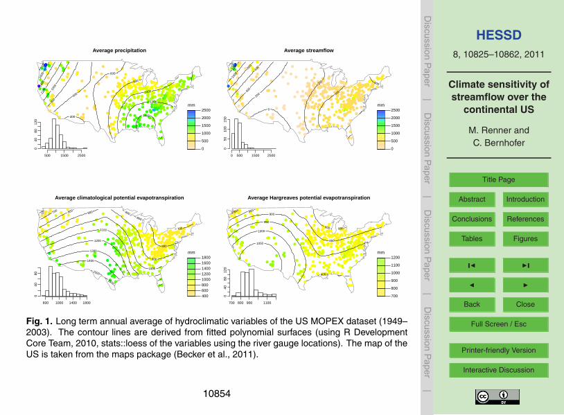
The basins in the US MOPEX dataset cover a variety of hydro-climatic conditions,which can be seen in the mapping of long-term average variables (P , Q, Ep,clim,Ep,Hargreaves) in Fig. 1. The basins with most precipitation are found in the Northwest,the Southeast and along the east coast. The central part of the US receives consider-able less precipitation, which is a continental climate effect intensified by the mountain20

ranges in the west and east, blocking west to east atmospheric moisture transport.Potential evapotranspiration obeys a north to south increasing gradient, which is mod-ulated by the continental climate in the Central US. The bottom maps display the differ-ence in Ep estimates, whereby the Hargreaves values, which are used further on, areless variable than the climatological Ep estimates.25

10835





HESSD8, 10825–10862, 2011


continental US


Title Page



Tables Figures

J I

J I

Back Close

Full Screen / Esc



Discussion

Paper

|D

iscussionP

aper|

Discussion

Paper

|D

iscussionP

aper|

Streamflow is naturally governed by precipitation input and follows the spatial pat-terns of precipitation. However, the arid conditions in the Central US result in lowerstreamflow amounts. This functional dependency can be seen in the Budyko plot inthe left panel of Fig. 2, plotting the evaporation ratio ET/P as function of the aridityindex Ep/P . In general, the basins follow the Budyko Hypothesis, whereby Ol’Dekop’s5

function explains 50 % of the variance. The aridity index of the basins ranges between0.27 and 4.51, with most basins clustering around 1. The right panel of Fig. 2 displaysthe relationship of the nondimensional measures W and U , referred to as UW space.Note, that W =1− ET

P , whereby ET/P is used in the Budyko plot on the ordinate. A thor-ough discussion of the relationship between both spaces can be found in Renner et al.10

(2011). The hydro-climatic data covers the UW space, meaning that there is a largevariety of hydro-climate conditions in the dataset. W is ranging between 0 and 1, whileU also shows a few negative values. This is due to two main reasons, (i) an underes-timation of the energy supply, i.e. in Ep and (ii) a physical reason, where advection ofheat into the basins leads to an additional input of energy for actual evapotranspiration.15

As we use the Hargreaves Ep estimates, the first reason is most likely.

4.2 Climate sensitivity of streamflow

Figure 3 provides a map of the climate sensitivity coefficients using the CCUW ap-proach, i.e. applying Eq. (6) on the long-term average values of P , Ep, Q. For example,a sensitivity coefficient of 2 implies that a relative change in precipitation results in20

a two times larger relative change in streamflow. Within the US most coefficients rangebetween 1.5 and 2.5. But there are also very high estimates, where a small change inannual precipitation would imply very pronounced relative changes in streamflow. Thisis due to the small amount of streamflow compared to precipitation and evapotranspi-ration in these predominantly arid catchments. Although there is some correlation of25

the sensitivity coefficient to the aridity index (Pearson correlation coefficient ρ= 0.52),we note that the inverse of the runoff ratio (P/Q) is the main controlling factor in deter-mining runoff sensitivity to climate (ρ=0.99).

10836





HESSD8, 10825–10862, 2011


continental US


Title Page



Tables Figures

J I

J I

Back Close

Full Screen / Esc



Discussion

Paper

|D

iscussionP

aper|

Discussion

Paper

|D

iscussionP

aper|

To further illustrate this functional relationship, we plot εQ,P in Fig. 4 as a functionof the evaporation ratio, which is directly related to the inverse of the runoff ratio, butbounded between 0 and 1. From the left panel (black dots) we see that the estimateof the CCUW method (εQ,P ;CCUW) is primarily and nonlinearly determined by ET/P . Toestimate the uncertainty in estimation of εQ,P ;CCUW, we computed εQ,P ;CCUW for each5

year of the annual time series and display the interquartile range (25–75 % percentilerange) of all those annual sensitivity coefficients as vertical grey line. The uncertaintyrange increases with ET/P . For values of ET/P > 0.6, the ranges get more apparentwith about 25 % of εQ,P , which can be up to the order of εQ,P for ET/P > 0.8. Thisimplies, the smaller the runoff ratio of a given basin the larger is the sensitivity to10

climate variations and the uncertainty in its estimation. Moreover, the variability inclimatic forcing of individual years or periods can have large impacts on the resultingstreamflow.

The right panel of Fig. 4 provides a comparison of the sensitivity estimates of CCUWwith the non-parametric Budyko approaches and the parametric Budyko function ap-15

proach of Roderick and Farquhar (2011). We find that the non-parametric Budykosensitivity approaches are determined by aridity only and show large differences toCCUW, already at medium values of ET/P . The parametric Budyko function approach(Mezentsev) yields similar sensitivities as the CCUW approach for ET/P < 0.9. This isdue to the parameter n, which inherently includes some dependency to ET/P . How-20

ever, it can be shown that there is an upper limit for the sensitivity coefficient which isset by n+1. Here, we estimated the largest value of n for the given dataset with n=9.1and the largest sensitivity with εQ,P,mez = 6.4. In contrast, the sensitivity of streamflowto precipitation, estimated by the CCUW approach is not bounded and proportionalto the inverse of the runoff ratio. This relationship is already expected by the more25

general definition of streamflow sensitivity Eq. (8). This behaviour is also discussed inSankarasubramanian and Vogel (2003), Yang and Yang (2011) and observed by Chiew(2006) for Australian basins, using a hydrological model.

10837





HESSD8, 10825–10862, 2011


continental US


Title Page



Tables Figures

J I

J I

Back Close

Full Screen / Esc



Discussion

Paper

|D

iscussionP

aper|

Discussion

Paper

|D

iscussionP

aper|

4.3 Assessment of observed and predicted changes in streamflow

Next, we evaluate the introduced analytical streamflow change prediction methods un-der past hydro-climatic changes in the contiguous US using data covering the wateryears from 1949 to 2003. As the approaches assume steady-state conditions, we eval-uate the changes by subdividing the data into two periods, 1949–1970 and 1971–2003.5

This choice is in accordance with the recent study of Wang and Hejazi (2011). Theyjustify their selection with a probable step increase in precipitation and in streamflow inlarge parts of the US around the year 1970 (McCabe and Wolock, 2002). First, we givean overview of the observed hydro-climatic changes and then evaluate the predictionsof streamflow changes. Last, we employ the conceptual model of Tomer and Schilling10

(2009) to attribute impacts of climate and basin characteristic changes.

4.3.1 Hydro-climatic changes in the US

We describe the climatic changes by comparing long-term average data of the twoperiods 1949–1970 and 1971–2003. Analysing the difference of the average annualrainfall, we find an increase in P for most basins, whereby the increase is significant for15

31 % of the basins (α = 0.05, Welch two sample t-test with unknown variance, using(R Development Core Team, 2010, stats::t.test)). The topleft map in Fig. 5 displaysthe spatial distribution of changes in P , which are largest over the Mississippi Riverbasin (>90 mm, excluding the Missouri River basin). Significant changes in precipita-tion are scattered over parts of the Mississippi basin and in the Northeast, however,20

there are hardly any significant changes in the peninsula of Florida and the West. Thedrastic increase in precipitation has already been discussed in many publications, (e.g.Lettenmaier et al., 1994; Milly and Dunne, 2001; Krakauer and Fung, 2008).

There are also significant changes in Ep, estimated by the Hargreaves equation.Here, we find a significant decline for 69 % of the basins. The topright map in Fig. 525

shows that the decrease is largest in the west of the Appalachian Mountain ranges

10838





HESSD8, 10825–10862, 2011


continental US


Title Page



Tables Figures

J I

J I

Back Close

Full Screen / Esc



Discussion

Paper

|D

iscussionP

aper|

Discussion

Paper

|D

iscussionP

aper|

(about −30 mm). These changes are directly related to a decrease in the diurnal tem-perature range, which is also reported by Lettenmaier et al. (1994).

Both, the increase in precipitation and the decrease in potential evapotranspirationshould ideally lead to an increase in annual streamflow. We find that 31 % of thebasins show a significant increase. The map in the bottomleft panel of Fig. 5 shows,5

that basins with significant increases in streamflow are predominantly found within theUpper Mississippi River basin and the Northern Appalachian Mountains and a fewbasins at the southern coast. These basins show an increase of about 41 % comparedto the average of the first period. For most of the other regions, we find non-significantstreamflow increases, while in the West there are mainly non-significant declines in10

annual streamflow. Please note, that we do not display basins when more than 10 yrof data are missing (78 basins) and that we removed 2 basins from further analysis,because the water balance was suspect (Q>P ).

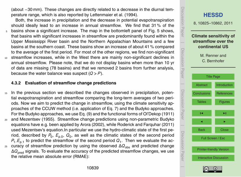
4.3.2 Evaluation of streamflow change predictions

In the previous section we described the changes observed in precipitation, poten-15

tial evapotranspiration and streamflow comparing the long-term averages of two peri-ods. Now we aim to predict the change in streamflow, using the climate sensitivity ap-proaches of the CCUW method (i.e. application of Eq. 7) and the Budyko approaches.For the Budyko approaches, we use Eq. (9) and the functional forms of Ol’Dekop (1911)and Mezentsev (1955). Streamflow change predictions using non-parametric Budyko20

equations have e.g. been applied by Arora (2002), while Roderick and Farquhar (2011)used Mezentsev’s equation.In particular we use the hydro-climatic state of the first pe-riod, described by P0, Ep,0, Q0, as well as the climatic states of the second periodP1,Ep,1 to predict the streamflow of the second period Q1. Then we evaluate the ac-curacy of streamflow prediction by using the observed ∆Qobs and predicted change25

∆Qpred signals. To evaluate the accuracy of the predicted streamflow changes, we usethe relative mean absolute error (RMAE):

10839





HESSD8, 10825–10862, 2011


continental US


Title Page



Tables Figures

J I

J I

Back Close

Full Screen / Esc



Discussion

Paper

|D

iscussionP

aper|

Discussion

Paper

|D

iscussionP

aper|

RMAE=

∑|∆Qobs−∆Qpred|∑

|∆Qobs|. (11)

The RMAE is zero when predictions actually match the observations, while a value of1 means a prediction error of 100 %.

The streamflow change prediction approaches are similar in performance, when con-sidering the whole dataset (RMAE = 50 %, 51 %, 51 % for CCUW, Mezentsev, and5

Ol’Dekop, respectively). A scatterplot of predicted versus observed changes is shownin the left panel of Fig. 6, where dots close to the 1 : 1 line indicate good predictions.While most dots scatter around the 1 : 1 line, there is a considerable number of basinswhere prediction and observation are completely different. There is also no indicationif one method is more realistic than the other.10

However, when sorting the results by prediction accuracy, we find that CCUW isslightly better than the Budyko approaches. About 16 % (28 %, 55 %) of the basinshave a RMAE prediction error smaller than 5 % (10 %, 20 %), while using the Budykohypothesis with the parametric function of Mezentsev yields 14 % (26 %, 52 %) andOldekop’s function 12 % (26 %, 52 %). That means by only considering climatic forcing15

changes, we are able to predict streamflow changes with an error smaller than 20 %for about 55 % of the basins.

The bottomright map in Fig. 5 presents the predicted streamflow changes by theCCUW method. There is an eye catching similarity of the spatial pattern of precipitationchanges shown in the topleft map. Comparing the predicted changes with the observed20

changes in streamflow in the bottomleft map, we see that there is a good coherencefrom the East to the Central US. Towards the Northwest, the predicted changes aresignificantly larger than the observed changes. However, the topleft map in Fig. 5shows that although there has been an increase in precipitation in the West, hardly anyof these changes have been significant. This may have important implications for the25

prediction methods considered here, which only deal with average climate conditionsand disregard interannual variability. In fact, a non-significant change in precipitation

10840





HESSD8, 10825–10862, 2011


continental US


Title Page



Tables Figures

J I

J I

Back Close

Full Screen / Esc



Discussion

Paper

|D

iscussionP

aper|

Discussion

Paper

|D

iscussionP

aper|

eventually does not justify to assume a change in average annual precipitation, whichis used as input to estimate some change in streamflow.

Next we assume, that the difference between observed and predicted (i.e. due toclimatic changes) change in streamflow can be attributed to changes in basin charac-teristics. With that we get an estimate of impacts of basin changes from the CCUW5

method and compare it with the results obtained by the method of Wang and Hejazi(2011). This comparison is shown as scatterplot in the right panel of Fig. 6. Thegraph indicates that there is a general agreement between both estimates (ρ= 0.97),although they are derived from different theoretical frameworks. In general, basins witha low evaporation ratio tend to show negative changes due to basin change, while10

basins with larger evaporation ratios show positive changes in streamflow. The largestdifferences between both methods are found for basins with very high evaporation ra-tios. In this case CCUW predicts larger changes than the Budyko approaches, whichwas already discussed above. These changes are small in absolute values, but quitelarge when seen relative to the annual totals of streamflow.15

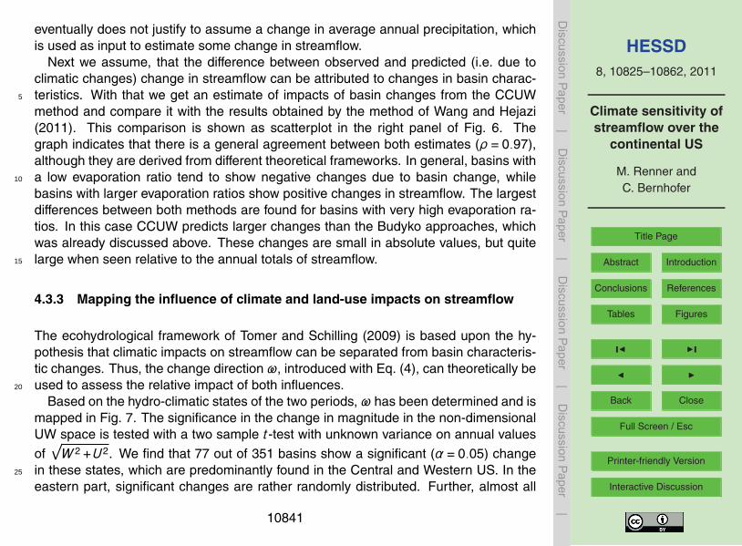
4.3.3 Mapping the influence of climate and land-use impacts on streamflow

The ecohydrological framework of Tomer and Schilling (2009) is based upon the hy-pothesis that climatic impacts on streamflow can be separated from basin characteris-tic changes. Thus, the change direction ω, introduced with Eq. (4), can theoretically beused to assess the relative impact of both influences.20

Based on the hydro-climatic states of the two periods, ω has been determined and ismapped in Fig. 7. The significance in the change in magnitude in the non-dimensionalUW space is tested with a two sample t-test with unknown variance on annual values

of√W 2+U2. We find that 77 out of 351 basins show a significant (α = 0.05) change

in these states, which are predominantly found in the Central and Western US. In the25

eastern part, significant changes are rather randomly distributed. Further, almost all

10841





HESSD8, 10825–10862, 2011


continental US


Title Page



Tables Figures

J I

J I

Back Close

Full Screen / Esc



Discussion

Paper

|D

iscussionP

aper|

Discussion

Paper

|D

iscussionP

aper|

basins with significant changes appear to be influenced by basin characteristic changes(i.e ω 6=135◦,315◦).

From the inlay histogram showing the frequency of observed change directions wesee that the majority of basins is right of the positive diagonal. This implies, the readermay also refer to Renner et al. (2011, Fig. 1), that there is a climate trend towards5

decreased aridity (Ep/P ) in 94 % of the basins.Regarding catchment efficiency Eq. (5), there are three main change scenarios: con-

stant CE, i.e. relative excess water W increases by the same amount as relative excessenergy U is decreased (case i), increasing CE when ∆U >∆W (case ii), or a declinein CE when ∆U <∆W . If we consider a segment of 45◦ centered at ω = 315◦ this10

would reflect roughly constant CE and valid conditions for the CCUW hypothesis. About31 % of the basins are actually within this boundary. According to the map in Fig. 7,these basins are found mainly in the central part below the Great Lakes, along a bandfollowing the Appalachian Mountains, and a few single basins in the West. Basinswith distinct climate impacts and improving CE (case iii, a segment of 45◦ centered15

at ω= 270◦) are most frequent (35 %) and found throughout the US. Almost all basinswithin the Great Plains and the West show constant or decreasing runoff and increas-ing ET. This is in accordance with the findings of Walter et al. (2004), who detectedpositive trends in ET but not in Q for western river basins (Columbia, Colorado andSacramento River basins). These trends may be linked to intraseasonal changes in20

hydrology, triggered by higher winter temperatures and thus less snow, which is melt-ing earlier (Barnett et al., 2008). Moreover, groundwater pumping for irrigation in theHigh Plains (McGuire, 2009) possibly contributed to the observed signals (Kustu et al.,2010).

From the map in Fig. 7 we see a transition of changes in CE over the Mississippi River25

basin. While the western part shows increasing CE, the central part remained mainlyconstant and the northern part shows large clusters of basins with a decline in CE. Thistransition may be primarily linked to the precipitation changes, which also show a westto east gradient (cf. map in Fig. 5). But agricultural cultivation, especially in basins of

10842





HESSD8, 10825–10862, 2011


continental US


Title Page



Tables Figures

J I

J I

Back Close

Full Screen / Esc



Discussion

Paper

|D

iscussionP

aper|

Discussion

Paper

|D

iscussionP

aper|

the US Midwest, may have amplified these trends. Most likely the additional rain couldnot increase evapotranspiration as a lack of soil water storage due to intensive tiledrainage (up to 30 % of the total state areas in the Midwest are drained Pavelis, 1987).So, the intensive agricultural land management did not only increased streamflow onaverage, but also lead to immense nitrogen leaching of Midwestern soils (Dinnes et al.,5

2002), showing biochemical signals far downstream (Raymond et al., 2008; Turner andRabalais, 1994).

Towards the East, changes in ω are spatially more heterogeneous. This is probablybecause topography and landuse are more diverse compared to the West, however,it is important to note, that the density of river gauge records is much larger. Most10

basins east of −87◦ latitude show increasing CE (case ii, 40 %) and constant CE (caseii, 36 %). Basins with decreasing CE occur rather local (case iii, 16 %).

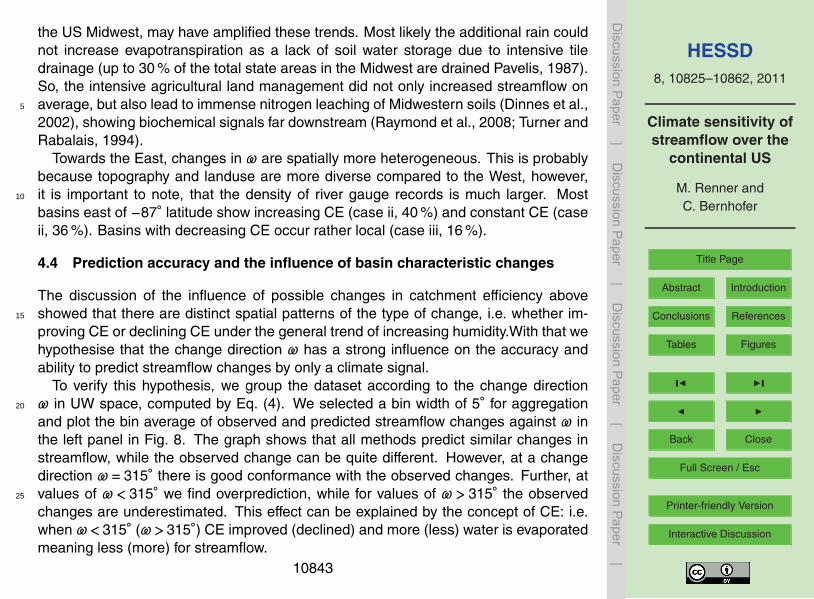
4.4 Prediction accuracy and the influence of basin characteristic changes

The discussion of the influence of possible changes in catchment efficiency aboveshowed that there are distinct spatial patterns of the type of change, i.e. whether im-15

proving CE or declining CE under the general trend of increasing humidity.With that wehypothesise that the change direction ω has a strong influence on the accuracy andability to predict streamflow changes by only a climate signal.

To verify this hypothesis, we group the dataset according to the change directionω in UW space, computed by Eq. (4). We selected a bin width of 5◦ for aggregation20

and plot the bin average of observed and predicted streamflow changes against ω inthe left panel in Fig. 8. The graph shows that all methods predict similar changes instreamflow, while the observed change can be quite different. However, at a changedirection ω= 315◦ there is good conformance with the observed changes. Further, atvalues of ω< 315◦ we find overprediction, while for values of ω> 315◦ the observed25

changes are underestimated. This effect can be explained by the concept of CE: i.e.when ω<315◦ (ω>315◦) CE improved (declined) and more (less) water is evaporatedmeaning less (more) for streamflow.

10843





HESSD8, 10825–10862, 2011


continental US


Title Page



Tables Figures

J I

J I

Back Close

Full Screen / Esc



Discussion

Paper

|D

iscussionP

aper|

Discussion

Paper

|D

iscussionP

aper|

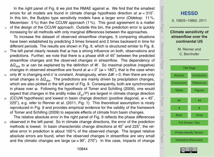
In the right panel of Fig. 8 we plot the RMAE against ω. We find that the smallesterrors for all models are found in climate change hypothesis direction at ω = 315◦.In this bin, the Budyko type sensitivity models have a larger error (Oldekop: 11 %,Mezentsev: 5 %) than the CCUW approach (1 %). This good agreement is a matterof the design of the CCUW approach. Outside this bin, the prediction error is quickly5

increasing for all methods with only marginal differences between the approaches.To increase the dataset of observed streamflow changes, 5 comparing situations

have been established by predicting 3 times forward and 2 times backward in time fordifferent periods. The results are shown in Fig. 9, which is structured similar to Fig. 8.The left panel clearly reveals that ω has a strong influence on both, observations and10

predictions. Further, we note that there is a phase shift of 45◦ between the predictedstreamflow changes and the observed changes in streamflow. The dependency of∆Qobs to ω can be explained by the definition of W . So maximal positive (negative)changes in observed streamflow are found at ω= 0◦ (ω= 180◦), that is the case whenonly W is changing and U is constant. Analogously, when ∆W = 0, then there are only15

small changes in ∆Qobs. The predictions are mainly driven by precipitation changes,which are also plotted in the left panel of Fig. 9. Consequently, both are synchronisedin phase over ω. Following the hypothesis of Tomer and Schilling (2009), one wouldexpect that changes in the aridity index (Ep/P ) are largest in climate change direction(CCUW hypothesis) and lowest in basin change direction (positive diagonal, ω= 45◦,20

225◦), e.g. refer to Renner et al. (2011, Fig. 1). This theoretical assumption is nicelyreproduced in Fig. 9 and provides empirical evidence for the validity of the frameworkof Tomer and Schilling (2009) to separate effects of climate from basin changes.

The relative absolute error in the right panel of Fig. 9 reflects the phase differencesobserved in the left panel. So in climate change directions, the error of the prediction25

methods is lowest. In basin characteristic change directions at 45◦ and 225◦, the rel-ative error in prediction is about 100 % of the observed change. The largest relativeabsolute errors are found, when the observed changes in streamflow are very smalland the climatic changes are large (ω≈ 90◦, 270◦). In this case, impacts of change

10844





HESSD8, 10825–10862, 2011


continental US


Title Page



Tables Figures

J I

J I

Back Close

Full Screen / Esc



Discussion

Paper

|D

iscussionP

aper|

Discussion

Paper

|D

iscussionP

aper|

in basin characteristics compensate for the expected changes in streamflow due toclimate changes.

4.5 Uncertainty discussion

4.5.1 Limitations due to observational data

Both climatic sensitivity approaches are based on long-term average data. These input5

data are spatially aggregated to river basin averages from point data and evaporativedemand and ET are only indirectly observed. For example, Milly (1994) showed byan uncertainty analysis of input data to their Budyko based water balance model thatuncertainties in input data may explain the deviations from observed and modelleddischarge and evapotranspiration.10

Another issue is that net energy supply, i.e. net radiation balance data, is ideallyrequired. However, direct observations of net radiation are not available for the purposeto estimate long-term catchment averages throughout the US. Therefore, a practicalchoice is to use potential evapotranspiration models, which provide an estimate basedon available meteorological data. Here, we used the Hargreaves equation, which only15

requires data of minimum and maximum daily temperature. Therefore, our estimates ofchange in evaporative demand are entirely based on the trends in diurnal temperatureranges and mean temperature over the US.

There may be other causes of the change in energy supply which are not reflectedin the trend in diurnal temperature ranges. For example, changes in net long wave ra-20

diation as reported by Qian et al. (2007) or changes in the surface albedo due to landcover changes. While the latter can be attributed to basin characteristic changes, theformer requires better high resolution radiation and energy balance estimates (Milly,1994). These estimates may be available by using remote sensing products or reanal-ysis products for past periods. This is, however, out of the scope of this study.25

Still, we believe, that the main conclusions regarding the retrospective assessmentof hydro-climatic changes and their regional patters will not be altered significantly by

10845





HESSD8, 10825–10862, 2011


continental US


Title Page



Tables Figures

J I

J I

Back Close

Full Screen / Esc



Discussion

Paper

|D

iscussionP

aper|

Discussion

Paper

|D

iscussionP

aper|

using improved data for evaporative demand. First, the main signal is covered in thediurnal temperature range data and second, the observed changes in the partitioningof water and surface fluxes can be attributed to a much larger part to the change inprecipitation.

4.5.2 Uncertainties due to inherent assumptions5

While introducing the theoretical framework by Renner et al. (2011) and the Budykoframework, considerable assumptions have been placed which may be violated bymeasurement reality.

First, we have to regard the assumption that the storages of water and energy arezero, which may be violated but hard to discern. For example, Tomer and Schilling10

(2009) used very dry periods to separate the data for computing long-term averages.However, this relatively subjective method may also introduce other problems. Sec-ondly, we assume steady state conditions. Several processes may violate this as-sumption, resulting in a trend of ET over time (Donohue et al., 2007). Our results clearlyshow that any process related to a change in basin characteristics, may result in dy-15

namic state transitions whose impacts on evapotranspiration and thus streamflow canbe larger than impacts of climatic variations. So we found, that catchment efficiencyhas been widely increasing in the Western US. This represents a non-stationary transi-tion in the water and energy balances towards increasing actual evapotranspiration onthe cost of streamflow. Thereby, the effects of climate and basin characteristic changes20

on streamflow seem to be of equal magnitude and compensate for each other. In thecompanion paper we discussed the different assumptions on catchment efficiency andclimate changes. While the Budyko functions inherently assume, that CE is changingwith the aridity index, the CCUW method assumes CE to be constant. Here, we areunable to verify which assumption is correct, because of the multitude of possible other25

effects, especially the large impacts of basin characteristics change. However, the clearspatial distributions of the change direction ω is an indication that basin characteristicchanges result in larger effects, than the definition of hydro-climatic feedbacks.

10846





HESSD8, 10825–10862, 2011


continental US


Title Page



Tables Figures

J I

J I

Back Close

Full Screen / Esc



Discussion

Paper

|D

iscussionP

aper|

Discussion

Paper

|D

iscussionP

aper|

5 Conclusions

This paper demonstrates the applicability and usefulness of the coupled water-energybalance framework (CCUW) of Renner et al. (2011) for the problem of estimating thesensitivity of streamflow to changes in climate. To test and compare the CCUW frame-work with the Budyko framework we employed a large hydro-climatic dataset of the5

continental US, covering a variety of different climatic conditions (humid to arid) andbasin characteristics, ranging from flat to mountainous basins with land cover typesranging from desert over agriculture to forested basins.

Based on long-term average hydro-climatological data (P , Ep, Q), we estimated andmapped the sensitivity of streamflow to changes in annual precipitation. The main dis-10

tinction between the Budyko and the CCUW hypotheses is the functional dependencyof the sensitivity coefficients. The sensitivity coefficients estimated by the Budykoframework depend on the aridity index and the type of the Budyko function only. Incontrast the CCUW hypothesis, implies that climatic sensitivity of streamflow dependsto a large degree on the inverse of the runoff ratio, which is already expected from15

the general definition of the sensitivity coefficient. This fundamental difference mayresult in large differences, which are most prominent for basins where runoff is verysmall compared to annual precipitation. However, for most of the other basins bothapproaches agree fairly well.

Further, we evaluated the capability of the climate sensitivity approaches to pre-20

dict a change in streamflow, given observed variations in the climate of the secondpart of the 20th century. The combination with the conceptual framework of Tomerand Schilling (2009) to discern climate from basin characteristic changes impacts yieldcomprehensive insights in the hydro-climatic changes in the US. We can reinstate, thatincreased annual precipitation lead to increases of streamflow and evapotranspiration25

in general. However, our results provide evidence that changes in basin characteristicsinfluenced how the additional amount of water is partitioned at the surface. Particularlythe mapping of ω, describing changes in partitioning of water and energy fluxes at the

10847





HESSD8, 10825–10862, 2011


continental US


Title Page



Tables Figures

J I

J I

Back Close

Full Screen / Esc



Discussion

Paper

|D

iscussionP

aper|

Discussion

Paper

|D

iscussionP

aper|

land surface, yields a quick overview of dominant impacts on streamflow. The resultantpatterns are spatially coherent and in agreement with previous studies. The quanti-tative separation of impacts of basin changes on streamflow supports the hypothesisthat humans directly and indirectly alter water resources at the regional and large basinscale. Most prominent are changes in the seasonality of climate due to global green-5

house gas emissions (Thomson, 1995; Barnett et al., 2008) and intensified agriculturallanduse, especially by artificial drainage and irrigation. The results suggest that thedirection and magnitude of human impacts distinctly vary with climate, soil, landuseand hydrographic conditions.

Last, we tested how concurrent effects of basin and climate changes on streamflow,10

encoded in the change direction ω, influenced the accuracy in predicting streamflowchanges. We found that there is a clear dependency on prediction accuracy. So,generally all sensitivity methods yield minimal errors, when a climate change directionis evident, which is a solid argument for the applicability of the Budyko and the CCUWframeworks.15

The results show that both frameworks agree in prediction accuracy, but the im-pact of basin changes within this dataset is too large to assess which theory is betterthan the other. However, we argue that the CCUW method is superior to the Budykoframework, as it can be applied to any reasonable hydro-climatic state without anyparametrisation. Still, real changes in basin characteristics and uncertainties in data20

which are essentially attributed to basin characteristic changes, are not predictable. Sowe conclude, that these impacts play a role and one needs to know about these effects,when applying any kind of climatic sensitivity framework.

Acknowledgement. This work was kindly supported by Helmholtz Impulse and NetworkingFund through Helmholtz Interdisciplinary Graduate School for Environmental Research (HI-25

GRADE) (Bissinger and Kolditz, 2008). We thank Kristina Brust and Rico Kronenberg (TUDresden) for valuable comments on the manuscript. The analysis and graphs are made withFree Open Source Software (F.O.S.S.).

10848





HESSD8, 10825–10862, 2011


continental US


Title Page



Tables Figures

J I

J I

Back Close

Full Screen / Esc



Discussion

Paper

|D

iscussionP

aper|

Discussion

Paper

|D

iscussionP

aper|

References

Aguilar, C. and Polo, M. J.: Generating reference evapotranspiration surfaces from theHargreaves equation at watershed scale, Hydrol. Earth Syst. Sci., 15, 2495–2508,doi:10.5194/hess-15-2495-2011, 2011. 10834, 10835

Arnell, N.: Hydrology and Global Environmental Change, Prentice Hall, 2002. 108295

Arora, V.: The use of the aridity index to assess climate change effect on annual runoff, J.Hydrol., 265, 164–177, 2002. 10828, 10839

Barnett, T., Pierce, D., Hidalgo, H., Bonfils, C., Santer, B., Das, T., Bala, G., Wood, A., Nozawa,T., Mirin, A., Cayan, D., and M. D. D.: Human-induced changes in the hydrology of thewestern United States, Science, 319, 1080, doi:10.1126/science.1152538, 2008. 10842,10

10848Becker, R. A., Wilks, A. R., Brownrigg, R., and Minka, T. P.: Maps: Draw Geographical

Maps, R package version 2.2-1, http://CRA∼N.R-project.org/package=maps, last accessed:11 November 2011. 10854

Bissinger, V. and Kolditz, O.: Helmholtz Interdisciplinary Graduate School for Environmental15

Research (HIGRADE), GAIA, 17, 71–73, 2008. 10848Bloschl, G. and Montanari, A.: Climate change impacts – throwing the dice?, Hydrol. Process.,

24, 374–381, doi:10.1002/hyp.7574, 2010. 10827Chiew, F.: Estimation of rainfall elasticity of streamflow in Australia, Hydrol. Sci. J., 51, 613–625,

doi:10.1623/hysj.51.4.613, 2006. 1083720

Dinnes, D., Karlen, D., Jaynes, D., Kaspar, T., Hatfield, J., Colvin, T., and Cambardella, C.:Nitrogen management strategies to reduce nitrate leaching in tile-drained Midwestern soils,Agron. J., 94, 153–171, 2002. 10843

Donohue, R. J., Roderick, M. L., and McVicar, T. R.: On the importance of including veg-etation dynamics in Budyko’s hydrological model, Hydrol. Earth Syst. Sci., 11, 983–995,25

doi:10.5194/hess-11-983-2007, 2007. 10846Dooge, J.: Sensitivity of runoff to climate change: A Hortonian approach, B. Am. Meteorol.

Soc., 73, 2013–2024, 1992. 10828Farnsworth, R. and Thompson, E.: Mean monthly, seasonal, and annual pan evaporation for

the United States, NOAA Techn. Rept. NWS, 34, 1982. 1083430

Groisman, P., Knight, R., Karl, T., Easterling, D., Sun, B., and Lawrimore, J.: Contemporarychanges of the hydrological cycle over the contiguous United States: trends derived from in

10849





http://dx.doi.org/10.5194/hess-15-2495-2011

http://dx.doi.org/10.1126/science.1152538

http://CRA~N.R-project.org/package=maps

http://dx.doi.org/10.1002/hyp.7574

http://dx.doi.org/10.1623/hysj.51.4.613


HESSD8, 10825–10862, 2011


continental US


Title Page



Tables Figures

J I

J I

Back Close

Full Screen / Esc



Discussion

Paper

|D

iscussionP

aper|

Discussion

Paper

|D

iscussionP

aper|

situ observations, J. Hydrometeorol., 5, 64–85, 2004. 10828Hargreaves, G. and Allen, R.: History and evaluation of Hargreaves evapotranspiration equa-

tion, J. Irrig. Drain. Eng., 129, 53–63, 2003. 10834, 10835Hargreaves, G., Hargreaves, G., and Riley, J.: Irrigation water requirements for Senegal river

basin, J. Irrig. Drain. Eng., 111, 265–275, 1985. 108345

Klemes, V.: Conceptualization and scale in hydrology, J. Hydrol., 65, 1–23, 1983. 10827Kochendorfer, J. and Hubbart, J.: The roles of precipitation increases and rural land-use

changes in streamflow trends in the upper Mississippi River basin, Earth Interact., 14, 1–12, 2010. 10829

Krakauer, N. Y. and Fung, I.: Mapping and attribution of change in streamflow in the coter-10

minous United States, Hydrol. Earth Syst. Sci., 12, 1111–1120, doi:10.5194/hess-12-1111-2008, 2008. 10838

Kuhnel, V., Dooge, J., O’Kane, J., and Romanowicz, R.: Partial analysis applied to scale prob-lems in surface moisture fluxes, Surv. Geophys., 12, 221–247, 1991. 10832

Kustu, M., Fan, Y., and Robock, A.: Large-scale water cycle perturbation due to irrigation pump-15

ing in the US high plains: A synthesis of observed streamflow changes, J. Hydrol., 390,222–244, doi:10.1016/j.jhydrol.2010.06.045, 2010. 10842

Lettenmaier, D., Wood, E., and Wallis, J.: Hydro-climatological trends in the continental UnitedStates, 1948–1988, J. Climate, 7, 586–607, 1994. 10828, 10838, 10839

Lins, H. and Slack, J.: Streamflow trends in the United States, Geophys. Res. Lett., 26, 227–20

230, 1999. 10828McCabe, G. and Wolock, D.: A step increase in streamflow in the conterminous United States,

Geophys. Res. Lett., 29, 38–1, doi:10.1029/2002GL015999, 2002. 10838McGuire, V.: Water-level changes in the High Plains aquifer, predevelopment to 2007, 2005-06,

and 2006-07, Publications of the US Geological Survey, p.17, 2009. 1084225

Mezentsev, V.: More on the calculation of average total evaporation, Meteorol. Gidrol., 5, 24–26, 1955. 10833, 10837, 10839, 10840, 10853, 10859

Milly, P.: Climate, soil water storage, and the average annual water balance, Water Resour.Res., 30, 2143–2156, 1994. 10845

Milly, P. and Dunne, K.: Trends in evaporation and surface cooling in the Mississippi River basin,30

Geophys. Res. Lett., 28, 1219–1222, doi:10.1029/2000GL012321, 2001. 10838Ol’Dekop, E.: On evaporation from the surface of river basins, Transactions on meteorological

observations, University of Tartu, 4, 200, 1911. 10832, 10836, 10839, 10840, 10853

10850








http://dx.doi.org/10.1016/j.jhydrol.2010.06.045

http://dx.doi.org/10.1029/2002GL015999

http://dx.doi.org/10.1029/2000GL012321

HESSD8, 10825–10862, 2011


continental US


Title Page



Tables Figures

J I

J I

Back Close

Full Screen / Esc



Discussion

Paper

|D

iscussionP

aper|

Discussion

Paper

|D

iscussionP

aper|

Oudin, L., Andreassian, V., Lerat, J., and Michel, C.: Has land cover a significant impact onmean annual streamflow? An international assessment using 1508 catchments, J. Hydrol.,357, 303–316, doi:10.1016/j.jhydrol.2008.05.021, 2008. 10834

Pavelis, G.: Farm drainage in the United States: history, status, and prospects, Miscellaneouspublication/United States, Dept. of Agriculture, Washington, DC, 1987. 108435

Qian, T., Dai, A., and Trenberth, K.: Hydroclimatic trends in the Mississippi River basin from1948 to 2004, J. Climate, 20, 4599, 2007. 10845

R Development Core Team: R: A Language and Environment for Statistical Computing, R Foun-dation for Statistical Computing, Vienna, Austria, available at: http://www.R-project.org/, lastaccess: December 2011, ISBN 3-900051-07-0, 2010. 10838, 1085410

Raymond, P., Oh, N., Turner, R., and Broussard, W.: Anthropogenically enhanced fluxes of wa-ter and carbon from the Mississippi River, Nature, 451, 449–452, doi:10.1038/nature06505,2008. 10843

Renner, M., Seppelt, R., and Bernhofer, C.: A simple water-energy balance framework to pre-dict the sensitivity of streamflow to climate change, Hydrol. Earth Syst. Sci. Discuss., 8,15

8793–8830, doi:10.5194/hessd-8-8793-2011, 2011. 10826, 10828, 10829, 10830, 10831,10832, 10833, 10836, 10842, 10844, 10846, 10847

Roderick, M. and Farquhar, G.: A simple framework for relating variations in runoff to vari-ations in climatic conditions and catchment properties, Water Resour. Res., 47, W00G07,doi:10.1029/2010WR009826, 2011. 10828, 10833, 10837, 10839, 1085320

Sankarasubramanian, A. and Vogel, R.: Hydroclimatology of the continental United States,Geophys. Res. Lett., 30, 1363, 2003. 10837

Sankarasubramanian, A., Vogel, R., and Limbrunner, J.: Climate elasticity of streamflow in theUnited States, Water Resour. Res., 37, 1771–1781, 2001. 10828

Schaake, J., Cong, S., and Duan, Q.: The US MOPEX data set, IAHS publication, Wallingford,25

Oxfordshire, 307, 9–28, 2006. 10828, 10834Small, D., Islam, S., and Vogel, R.: Trends in precipitation and streamflow in the Eastern US:

paradox or perception, Geophys. Res. Lett., 33, L03403, doi:10.1029/2005GL024995, 2006.10828

Thomson, D.: The seasons, global temperature, and precession, Science, 268, 59–68, 1995.30

10848Tomer, M. and Schilling, K.: A simple approach to distinguish land-use and climate-change

effects on watershed hydrology, J. Hydrol., 376, 24–33, doi:10.1016/j.jhydrol.2009.07.029,

10851






http://www.R-project.org/

http://dx.doi.org/10.1038/nature06505

http://dx.doi.org/10.5194/hessd-8-8793-2011

http://dx.doi.org/10.1029/2010WR009826

http://dx.doi.org/10.1029/2005GL024995


HESSD8, 10825–10862, 2011


continental US


Title Page



Tables Figures

J I

J I

Back Close

Full Screen / Esc



Discussion

Paper

|D

iscussionP

aper|

Discussion

Paper

|D

iscussionP

aper|

2009. 10828, 10829, 10830, 10833, 10838, 10841, 10844, 10846, 10847Troch, P., Martinez, G., Pauwels, V., Durcik, M., Sivapalan, M., Harman, C., Brooks, P.,

Gupta, H., and Huxman, T.: Climate and vegetation water use efficiency at catchment scales,Hydrol. Process., 23, 2409–2414, doi:10.1002/hyp.7358, 2009. 10834

Turner, R. and Rabalais, N.: Coastal eutrophication near the Mississippi river delta, Nature,5

368, 619–621, 1994. 10843Voepel, H., Ruddell, B., Schumer, R., Troch, P. A., Brooks, P. D., Neal, A., Durcik, M.,

and Sivapalan, M.: Quantifying the role of climate and landscape characteristics onhydrologic partitioning and vegetation response, Water Resour. Res., 47, W00J09,doi:10.1029/2010WR009944, 2011. 1083410

Walter, M., Wilks, D., Parlange, J., and Schneider, R.: Increasing evapotranspiration from theconterminous United States, J. Hydrometeorol., 5, 405–408, 2004. 10828, 10842

Wang, D. and Cai, X.: Comparative study of climate and human impacts on sea-sonal baseflow in urban and agricultural watersheds, Geophys. Res. Lett., 37, L06406,doi:10.1029/2009GL041879, 2010. 1082915

Wang, D. and Hejazi, M.: Quantifying the relative contribution of the climate and direct humanimpacts on mean annual streamflow in the contiguous United States, Water Resour. Res., 47,W00J12, doi:10.1029/2010WR010283, 2011. 10829, 10833, 10834, 10838, 10841, 10859

Yang, H. and Yang, D.: Derivation of climate elasticity of runoff to assess the effects of climatechange on annual runoff, Water Resour. Res., 47, W07526, doi:10.1029/2010WR009287,20

2011. 10828, 10837

10852





http://dx.doi.org/10.1002/hyp.7358

http://dx.doi.org/10.1029/2010WR009944

http://dx.doi.org/10.1029/2009GL041879

http://dx.doi.org/10.1029/2010WR010283

http://dx.doi.org/10.1029/2010WR009287

HESSD8, 10825–10862, 2011


continental US


Title Page



Tables Figures

J I

J I

Back Close

Full Screen / Esc



Discussion

Paper

|D

iscussionP

aper|

Discussion

Paper

|D

iscussionP

aper|

Table 1. Budyko functions and their partial differentials as used in the text.

Budyko function ∂ET

∂P∂ET

∂EpReference

ET =Ep · tanh(

PEp

)1− tanh2

(PEp

)− P

Ep

(1− tanh2

(PEp

))+ tanh

(PEp

)Ol’Dekop (1911)

ET =Ep ·P

(P n+Enp )1/n

ET

P

(En

p

P n+Enp

)ET

Ep

(P n

P n+Enp

)Mezentsev (1955)

∂ET

∂n = ETn

(ln(P n+En

p )n − (P n ln(P )+En

p ln(Ep))

P n+Enp

)Roderick and Farquhar (2011)

10853





HESSD8, 10825–10862, 2011


continental US


Title Page



Tables Figures

J I

J I

Back Close

Full Screen / Esc



Discussion

Paper

|D

iscussionP

aper|

Discussion

Paper

|D

iscussionP

aper|

●●●●●

●

●

●●

● ●●●●●

●●●●●

●●

●●●●●●●●●

●●●●

●●●●●

●●

●●●●●

●●●

●●

●●●●●●●● ●

●●

●●●●●

●

●●●●●●

●

●

●●●

●

●

●●

●

● ●●

●●

●●●

●●●

●●

●

●●

●

● ●

●●●●●

●●●●●●●●●

●●●

●

●●

●●●●●●●●

●●●●●●●

●●

●●●●●

●●●●

●●

●●

●

●●●●

●

●●

●●●●●●●●

●

●●

●●●●●●

●●

●●

●●●●●

●●●

●

●

●●

●

●●● ●●●

●●●● ● ●●●●●

● ●

●

● ●●●

●●●

●●●●

●●●●

●●●

●●

●●●●●

●●●●

●●●●●●●

●

●●●

●●●●●●

●●●

●●

●

●

●

●● ●

●

●

●●●●●●●●●●

●●●

●

● ●●

●●●●

●●●●●●●

●●●

●●●

●

●●

●●●

●●

●●●

●● ●●

●●

●●

●●

●●●

●● ● ● ●

●●

●

● ●

●●●●

●

●●●●●

●●

●●

●●●

●●●●●●

●●

●

●

●●●

●●

●●

●

●●●●●

●

●●

●●●●

●

●

● ●●●●●

●●

●●

●●●●●

●

●

●●●●

●●

●●●●

●●●●●

●

●●

●●

●●

●

Average precipitation

400

600

600

800

800

100

0

1000

120

0

1200

140

0

1400

160

0

Fre

quen

cy

500 1500 2500

040

8012

0

0

500

1000

1500

2000

2500mm

●●●●●

●

●

●●

● ●●●●●

●●●●●

●●

●●●●●●●●●

●●●●

●●●●●

●●

●●●●●

●●●

●●

●●●●●●●● ●

●●

●●●●●

●

●●●●●●

●

●

●●●

●

●

●●

●

● ●●

●●

●●●

●●●

●●

●

●●

●

● ●

●●●●●

●●●●●●●●●

●●●

●

●●

●●●●●●●●

●●●●●●●

●●

●●●●●

●●●●

●●

●●

●

●●●●

●

●●

●●●●●●●●

●

●●

●●●●●●

●●

●●

●●●●●

●●●

●

●

●●

●

●●● ●●●

●●●● ● ●●●●●

● ●

●

● ●●●

●●●

●●●●

●●●●

●●●

●●

●●●●●

●●●●

●●●●●●●●●●

●●●●●●

●●●

●●

●

●

●

●● ●

●

●

●●●●●●●●●●

●●●

●

● ●●

●●●●

●●●●●●●

●●●

●●●

●

●●

●●●

●●

●●●

●● ●●

●●

●●

●●

●●●

●● ● ● ●

●●

●

● ●

●●●●

●

●●●●●

●●

●●

●●●

●●●●●●

●●

●

●

●●●

●●

●●

●

●●●●●

●

●●

●●●●

●

●

● ●●●●●

●●

●●

●●●●●

●

●

●●●●

●●

●●●●

●●●●●

●

●●

●●

●●

●

Average streamflow

0

200

200

400

400

600

600

800

100

0

120

0

Fre

quen

cy

0 500 1500 2500

050

100

150

0

500

1000

1500

2000

2500mm

●●●●

●

●

●●

● ●●●●●

●●●●●

●●

●●●●●●●●●

●●●●

●●●●●

●●

●●●●●

●●●

●●

●●●●●●●● ●

●●

●●●●●

●

●●●●●●

●

●

●●●

●

●

●●

●

● ●●

●●

●●●

●●●

●●

●

●●

●

● ●

●●●●●

●●●●●●●●●

●●●

●

●●

●●●●●●●●

●●●●●●●

●●

●●●●●

●●●●

●●

●●

●

●●●●

●

●●

●●●●●●●●

●

●●

●●●●●●

●●

●●

●●●●●

●●●

●

●

●●

●

●●● ●●

●●●● ● ●●●●●

● ●

●

● ●●●

●●●

●●●●

●●●●

●●●

●●

●●●●●

●●●●

●●●●●●●

●

●●●

●●●●●●

●●●

●●

●

●

●

●● ●

●

●

●●●●●●●●●●

●●●

●

● ●●

●●●●

●●●●●●●

●●●

●●●

●

●●

●●●

●●

●●●

●● ●●

●●

●●

●●

●●●

●● ● ● ●

●●

●

● ●

●●●●

●

●●●●●

●●

●●

●●●

●●●●●●

●●

●

●

●●●

●●

●●

●

●●●●●

●

●●

●●●

●

●

● ●●●●●

●●

●●

●●●●●

●

●

●●●●

●●

●●●●

●●●●●

●

●●

●●

●●

●

Average climatological potential evapotranspiration

700

700

800 800 800

800

900

900

1000

1100

1200

1300

1400

1500

1500

Fre

quen

cy

600 1000 1400 1800

040

80

40060080010001200140016001800

mm

●●●●●

●

●

●●

● ●●●●●

●●●●●

●●

●●●●●●●●●

●●●●

●●●●●

●●

●●●●●

●●●

●●

●●●●●●●● ●

●●

●●●●●

●

●●●●●●

●

●

●●●

●

●

●●

●

● ●●

●●

●●●

●●●

●●

●

●●

●

● ●

●●●●●

●●●●●●●●●

●●●

●

●●

●●●●●●●●

●●●●●●●

●●

●●●●●

●●●●

●●

●●

●

●●●●

●

●●

●●●●●●●●

●

●●

●●●●●●

●●

●●

●●●●●

●●●

●

●

●●

●

●●● ●●●

●●●● ● ●●●●●

● ●

●

● ●●●

●●●

●●●●

●●●●

●●●

●●

●●●●●

●●●●

●●●●●●●

●

●●●

●●●●●●

●●●

●●

●

●

●

●● ●

●

●

●●●●●●●●●●

●●●

●

● ●●

●●●●

●●●●●●●

●●●

●●●

●

●●

●●●

●●

●●●

●● ●●

●●

●●

●●

●●●

●● ● ● ●

●●

●

● ●

●●●●

●

●●●●●

●●

●●

●●●

●●●●●●

●●

●

●

●●●

●●

●●

●

●●●●●

●

●●

●●●●

●

●

● ●●●●●

●●

●●

●●●●●

●

●

●●●●

●●

●●●●

●●●●●

●

●●

●●

●●

●

Average Hargreaves potential evapotranspiration

800

800 800

850

850

900

900

950

1000

1050

Fre

quen

cy

700 800 900 1100

040

8012

0

700

800

900

1000

1100

1200mm

Fig. 1. Long term annual average of hydroclimatic variables of the US MOPEX dataset (1949–2003). The contour lines are derived from fitted polynomial surfaces (using R DevelopmentCore Team, 2010, stats::loess of the variables using the river gauge locations). The map of theUS is taken from the maps package (Becker et al., 2011).

10854





HESSD8, 10825–10862, 2011


continental US


Title Page



Tables Figures

J I

J I

Back Close

Full Screen / Esc



Discussion

Paper

|D

iscussionP

aper|

Discussion

Paper

|D

iscussionP

aper|

●●

●

●●

●

●

●

●

●●

●

●

●

●

●●

●

●

●●

●

●●●

●

●

●●●

●

●

●●

●

●

●

●●

●●

●

●

●●●

●●●

●

●●●●●●●●

●●

●●

●

●●

●

●●●

●

●

●

●●

●

●

●

●●●

●

●

●

●

●

●

●●

●●

●●●

●

●

●

●●●●

●

●●

●

●●

●●

●

●

●●

●●

●●●

●

●●

●

●

●

●

●

●●

●

●

●

●●

●●●●

●

●●

●●●

●●●●

●●●●

●

●

●

●

●

●●

●

●●

●●

●

●

●●●●●●

●

●

●

●

●

●

●

●

●●●

●

●

●

●●

●●

●

●●

●

●

●

●●

●●

●

●

●

●

●

●●●●

●●

●

●●

●

●

●

●

●●●●●●

●

●●●●●●●●

●●●●

●

●●●●

●

●●●

●

●●●●

●●●●

●

●

●●●●●

●●●

●

●

●

●●●

●

●●

●

●

●●●

●

●●

●●●●●

●

● ●

●●

●●●

●

●

●

●

●

●●●●

●●●

●●

●

●●

●

●

●

●

●

●

●●

●●

●●

●●

●●●

●

●●

●●

●

●

●

●●

●

●

●

●

●●●●

●

●

●●●●

●●

●

●

● ●

●●●

●

●●

●

●

● ●

●

●

●

●

● ●

●●

●

●

●

●

●

●

●

●

●

●

●

●●

●

●

●

●

●

●

●

●

●

●

●

●

●

●

●●

●

●

●

●●

●

●

●

●

●

●

●

●

●●●

●

●●

●

●

●

●

●

●

●

0 1 2 3 4 5

0.0

0.2

0.4

0.6

0.8

1.0

Ep P

ET

P

water limit

ener

gy li

mit

●●

●

●●

●

●

●

●

●●

●

●

●

●

●●

●

●

●●

●

●●●

●

●

●●●

●

●

●●

●

●

●

●●

●●

●

●

●●●

●●●

●

●●●●●●●●

●●

●●

●

●●

●

●●●

●

●

●

●●

●

●

●

●●●

●

●

●

●

●

●

●●

●●

●●●

●

●

●

●●●●

●

●●

●

●●

●●

●

●

●●

●●

●●●

●

●●

●

●

●

●

●

●●

●

●

●

●●

●●●●

●

●●

●●●

●●●●

●●●●

●

●

●

●

●

●●

●

●●

●●

●

●

●●●●●●

●

●

●

●

●

●

●

●

●●●

●

●

●

●●

●●

●

●●

●

●

●

●●

●●

●

●

●

●

●

●●●●

●●

●

●●

●

●

●

●

●●●●●●

●

●●●●●●●●

●●●●

●

●●●●

●

●●●

●

●●●●

●●●●

●

●

●●●●●

●●●

●

●

●

●●●

●

●●

●

●

●●●

●

●●

●●●●●

●

● ●

●●

●●●

●

●

●

●

●

●●●●

●●●

●●

●

●●

●

●

●

●

●

●

●●

●●

●●

●●

●●●

●

●●

●●

●

●

●

●●

●

●

●

●

●●●●

●

●

●●●●

●●

●

●

● ●

●●●

●

●●

●

●

● ●

●

●

●

●

● ●

●●

●

●

●

●

●

●

●

●

●

●

●

●●

●

●

●

●

●

●

●

●

●

●

●

●

●

●

●●

●

●

●

●●

●

●

●

●

●

●

●

●

●●●

●

●●

●

●

●

●

●

●

●

Oldekop function

●● ●

●

●

●

●

●●

●

●● ●

●

●

●

●

●

●

●●

●

●●●

●

●

●●●

●

●●●●

●

●

●

●●

●

●

●

●●●

●

●●●

●●

●●

●●●●

●●

●●●

●●

●

●

●●

●

●●

●●

●

●

● ●●

●

● ●

●●

●

●

●●

●● ●

●●

●

●

●

●●●●●●

●

●

●

●●●●

●

●

●

●

●

●●

●

●

●

●

●

●

●●

●

●●

●

●

● ●●

●

●●●

●

●●●

●●

●●

●●

●●●● ● ●

●

●

●●●

●

●

●

●●

●

●●●●●●●

●●

●●●●

●

●

●

●

●

●

●

●

●

●●

●

●

●

●

●

●

●●

●

●●●

●●

●

●

●

●●●

●

●

●

●●● ●

● ●●●

●●●●

●●●

●

●●●●

●

●●●●

● ●●●●

●●

●●

●

●●●●

●●●●

●

●

●●●●

● ●●

●

●●

●

●

●

●●

●

●

●●

●●●

●

●●●

●

●●●●

●

●

●

●

●

●●

●●

●●

●●●●

●

●●

●

●

●

●

●● ●

●

●

●

●

●

●●

●

●

●●

●

●

●

●●

● ●●

●●

●

● ●

●

●

●

●

●

●

●●●

●

●

●

●●

●●

●

●

●

●

●

●

●

●●

●

●● ●

●

●

●

●

●

●●

●

●●

●

●

●●

●

●

●●

●

●

●

●

●●

●

●

●

●

●●

●

●

●

●

●

●

●

●

●

●

●

●

●

●●

●●

●

●

●

●

●

●

●

●

●

●

●

●

●

●

●

●

●

●

●

−0.2 0.0 0.2 0.4 0.6 0.8 1.0

−0.

20.

00.

20.

40.

60.

81.

0W = Q/P

U =

1 −

ET

Ep

wat

er li

mit

energy limit

●● ●

●

●

●

●

●●

●

●● ●

●

●

●

●

●

●

●●

●

●●●

●

●

●●●

●

●●●●

●

●

●

●●

●

●

●

●●●

●

●●●

●●

●●

●●●●

●●

●●●

●●

●

●

●●

●

●●

●●

●

●

● ●●

●

● ●

●●

●

●

●●

●● ●

●●

●

●

●

●●●●●●

●

●

●

●●●●

●

●

●

●

●

●●

●

●

●

●

●

●

●●

●

●●

●

●

● ●●

●

●●●

●

●●●

●●

●●

●●

●●●● ● ●

●

●

●●●

●

●

●

●●

●

●●●●●●●

●●

●●●●

●

●

●

●

●

●

●

●

●

●●

●

●

●

●

●

●

●●

●

●●●

●●

●

●

●

●●●

●

●

●

●●● ●

● ●●●

●●●●

●●●

●

●●●●

●

●●●●

● ●●●●

●●

●●

●

●●●●

●●●●

●

●

●●●●

● ●●

●

●●

●

●

●

●●

●

●

●●

●●●

●

●●●

●

●●●●

●

●

●

●

●

●●

●●

●●

●●●●

●

●●

●

●

●

●

●● ●

●

●

●

●

●

●●

●

●

●●

●

●

●

●●

● ●●

●●

●

● ●

●

●

●

●

●

●

●●●

●

●

●

●●

●●

●

●

●

●

●

●

●

●●

●

●● ●

●

●

●

●

●

●●

●

●●

●

●

●●

●

●

●●

●

●

●

●

●●

●

●

●

●

●●

●

●

●

●

●

●

●

●

●

●

●

●

●

●●

●●

●

●

●

●

●

●

●

●

●

●

●

●

●

●

●

●

●

●

●

012345

Ep P

Fig. 2. Budyko (left) and UW space (right) plots of the period (1949–2003) of the MOPEXdataset. Ep is computed by the Hargreaves method. The 1 : 1 line in the UW space diagramseparates areas with energy limitation (Ep/P < 1) and water limitation (Ep/P > 1). Grey linesindicate the water and energy limits.

10855





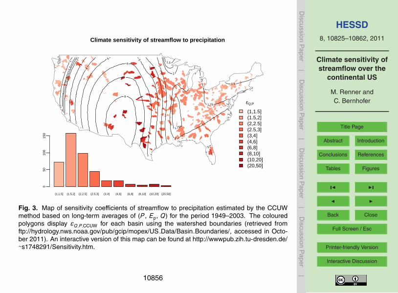
HESSD8, 10825–10862, 2011


continental US


Title Page



Tables Figures

J I

J I

Back Close

Full Screen / Esc



Discussion

Paper

|D

iscussionP

aper|

Discussion

Paper

|D

iscussionP

aper|

εQ,P

(1,1.5](1.5,2](2,2.5](2.5,3](3,4](4,6](6,8](8,10](10,20](20,50]

Climate sensitivity of streamflow to precipitation

1

1.5

1.5

1.5

1.7

5

1.75

1.75

1.75

2

2

2

3 3

3

4

4

5 5

6

7

8

(1,1.5] (1.5,2] (2,2.5] (2.5,3] (3,4] (4,6] (6,8] (8,10] (10,20] (20,50]

050

100

150

Fig. 3. Map of sensitivity coefficients of streamflow to precipitation estimated by the CCUWmethod based on long-term averages of (P , Ep, Q) for the period 1949–2003. The colouredpolygons display εQ,P,CCUW for each basin using the watershed boundaries (retrieved fromftp://hydrology.nws.noaa.gov/pub/gcip/mopex/US Data/Basin Boundaries/, accessed in Octo-ber 2011). An interactive version of this map can be found at http://wwwpub.zih.tu-dresden.de/∼s1748291/Sensitivity.htm.

10856





ftp://hydrology.nws.noaa.gov/pub/gcip/mopex/US_Data/Basin_Boundaries/

http://wwwpub.zih.tu-dresden.de/~s1748291/Sensitivity.htm

http://wwwpub.zih.tu-dresden.de/~s1748291/Sensitivity.htm

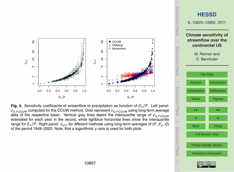
HESSD8, 10825–10862, 2011


continental US


Title Page



Tables Figures

J I

J I

Back Close

Full Screen / Esc



Discussion

Paper

|D

iscussionP

aper|

Discussion

Paper

|D

iscussionP

aper|

0.0 0.2 0.4 0.6 0.8 1.0

12

510

2050

ET P

ε Q,P

● ●●●●●

●●

●

●●

●●

●

●

●●

●

●

●●●

●●●● ●

●●●●

● ●● ●●

●

●●●●

●

●

●●●

●●●●

●●●●●●

●●

●●

●●

●

●●

●

●●

●

●

●●

●●

●

●

●

●●●

●

●

●

●

●

●●●

●●●●●

●●

●

●●●●

●

●●●

● ●●●●

●●●

●●●●●

●

●●

●

●●

●

●● ●

●●

●● ●●●●●

●

●●●●●●●●● ●●●

●

●●

●

●

●

●●

●

●●

●●

●●

●●●●●●

●

●●

●●

●

●

●●

●●

●

●●

●●●●●

● ●

●

● ●●●

●●●

●●

●

●

●●●●

●●

●●●

●

●

●

●

●●●

●●●●

●●●●●●●

●

●●●●

●

●●

●●

●

●●●

●

●●●●●●●

●

●

●

●●●●●

●●

●

●●

●

●●

●

●

●

●

●

●

●●●

●

●●

●●●

●●●

●

●

●

●

●

●

●

●

●

●

●

●

●●●●

●●●

●●

●

●●

●

●

●

●●

●

●●

●

●

●●

●●

●●

●

●●●

●

●

●

●

●●●

●●

●

●

●●

●●

●

●●●●●

●●

●

●

●●

●

●●

●

●●

●

●

●

●

●

●

●●

●

●

●

●

●

●●

●

●

●

●

●

●

●

●

● ●

●

●

●

●

●

●

●●

●

●

●

●●

●

●●●

●

●

●●

●

●

●● ●

●

● ●

●●●

●

●

●

●●

●

●

●●

●

0.0 0.2 0.4 0.6 0.8 1.0

12

510

2050

ET Pε Q

,P

● ●●●●●

●●

●

●●

●●

●

●

●●

●

●

●●●

●●●● ●

●●●●

● ●● ●●

●

●●●●

●

●

●●●

●●●●

●●●●●●

●●

●●

●●

●

●●

●

●●

●

●

●●

●●

●

●

●

●●●

●

●

●

●

●

●●●

●●●●●

●●

●

●●●●

●

●●●

● ●●●●

●●●

●●●●●

●

●●

●

●●

●

●● ●

●●

●● ●●●●●

●

●●●●●●●●● ●●●

●

●●

●

●

●

●●

●

●●

●●

●●

●●●●●●

●

●●

●●

●

●

●●

●●

●

●●

●●●●●

● ●

●

● ●●●

●●●

●●

●

●

●●●●

●●

●●●

●

●

●

●

●●●

●●●●

●●●●●●●

●

●●●●

●

●●

●●

●

●●●

●

●●●●●●●

●

●

●

●●●●●

●●

●

●●

●

●●

●

●

●

●

●

●

●●●

●

●●

●●●

●●●

●

●

●

●

●

●

●

●

●

●

●

●

●●●●

●●●

●●

●

●●

●

●

●

●●

●

●●

●

●

●●

●●

●●

●

●●●

●

●

●

●

●●●

●●

●

●

●●

●●

●

●●●●●

●●

●

●

●●

●

●●

●

●●

●

●

●

●

●

●

●●

●

●

●

●

●

●●

●

●

●

●

●

●

●

●

● ●

●

●

●

●

●

●

●●

●

●

●

●●

●

●●●

●

●

●●

●

●

●● ●

●

● ●

●●●

●

●

●

●●

●

●

●●

●

● CCUWOldekopMezentsev

Fig. 4. Sensitivity coefficients of streamflow to precipitation as function of ET/P . Left panel:εQ,P ;CCUW computed for the CCUW method. Dots represent εQ,P ;CCUW using long-term averagedata of the respective basin. Vertical grey lines depict the interquartile range of εQ,P ;CCUWestimated for each year in the record, while lightblue horizontal lines show the interquartilerange for ET/P . Right panel: εQ,P for different methods using long-term averages of (P , Ep, Q)of the period 1949–2003. Note, that a logarithmic y-axis is used for both plots.

10857





HESSD8, 10825–10862, 2011


continental US


Title Page



Tables Figures

J I

J I

Back Close

Full Screen / Esc



Discussion

Paper

|D

iscussionP

aper|

Discussion

Paper

|D

iscussionP

aper|

●●●●●

●

●

●●

● ●●●●●

●●●●●

●●

●●●●●●●●●

●●●●

●●●●●

●●

●●●●●

●●●

●●

●●●●●●●● ●

●●

●●●●●

●

●●●●●●

●

●

●●●

●

●

●●

●

● ●●

●●

●●●

●●●

●●

●

●●

●

● ●

●●●●●

●●●●●●●●●

●●●

●

●●

●●●●●●●●

●●●●●●●

●●

●●●●●

●●●●

●●

●●

●

●●●●

●

●●

●●●●●●●●

●

●●

●●●●●●

●●

●●

●●●●●

●●●

●

●

●●

●

●●● ●●●

●●●● ● ●●●●●

● ●

●

● ●●●

●●●

●●●●

●●●●

●●●

●●

●●●●●

●●●●

●●●●●●●

●

●●●

●●●●●●

●●●

●●

●

●

●

●● ●

●

●

●●●●●●●●●●

●●●

●

● ●●

●●●●

●●●●●●●

●●●

●●●

●

●●

●●●

●●

●●●

●● ●●

●●

●●

●●

●●●

●● ● ● ●

●●

●

● ●

●●●●

●

●●●●●

●●

●●

●●●

●●●●●●

●●

●

●

●●●

●●

●●

●

●●●●●

●

●●

●●●●

●

●

● ●●●●●

●●

●●

●●●●●

●

●

●●●●

●●

●●●●

●●●●●

●

●●

●●

●●

●

●●

●

●

●●

●●●

●●●

●●

●●

●●●●●●●●●●

●●●●

●●●●

●●●

●●●●●●●● ●

●●

●●

●●

●●

●

●●

●

● ●

●●●

●●●●

●●●●●

●

●

●

●●

● ● ●●●●●

● ●●● ●

●●●

●●●

●●●

●

●●

●

●

●

●● ●

●

●●●

● ●

●●●

●●●●●●

●

●

●

●●

●●●

●

●

Change in precipitation

20

40

40

60

60

60

60

80

80

100

100

120

120

140 140

Fre

quen

cy

−100 0 50 150 250

010

020

0

−100

−50

0

50

100

150

200∆P [mm]

●●●●●

●

●

●●

● ●●●●●

●●●●●

●●

●●●●●●●●●

●●●●

●●●●●

●●

●●●●●

●●●

●●

●●●●●●●● ●

●●

●●●●●

●

●●●●●●

●

●

●●●

●

●

●●

●

● ●●

●●

●●●

●●●

●●

●

●●

●

● ●

●●●●●

●●●●●●●●●

●●●

●

●●

●●●●●●●●

●●●●●●●

●●

●●●●●

●●●●

●●

●●

●

●●●●

●

●●

●●●●●●●●

●

●●

●●●●●●

●●

●●

●●●●●

●●●

●

●

●●

●

●●● ●●●

●●●● ● ●●●●●

● ●

●

● ●●●

●●●

●●●●

●●●●

●●●

●●

●●●●●

●●●●

●●●●●●●

●

●●●

●●●●●●

●●●

●●

●

●

●

●● ●

●

●

●●●●●●●●●●

●●●

●

● ●●

●●●●

●●●●●●●

●●●

●●●

●

●●

●●●

●●

●●●

●● ●●

●●

●●

●●

●●●

●● ● ● ●

●●

●

● ●

●●●●

●

●●●●●

●●

●●

●●●

●●●●●●

●●

●

●

●●●

●●

●●

●

●●●●●

●

●●

●●●●

●

●

● ●●●●●

●●

●●

●●●●●

●

●

●●●●

●●

●●●●

●●●●●

●

●●

●●

●●

●

●●●●

●

●● ●●●●

●●

●●

●●●●●●●

●●●●

●●●●●

●●

●●●●●● ●●●●●●●

●●

●●●●

●●●●●

●●●

●●

●●●● ●

●●●●●

●●●●●●●●●

●●●

●

●●

●

●●●●●●●

●●

●●●●●

●●●●

●●

●●

●

●●●●

●

●●

●●●●●●●●

●

●●●●

●●●●

●●●

●●

●

●●

●●●● ● ●●●●

●●●

●

●●

●●

●●

●●●

●●

●●●●

●●●●●●

●

●●●

●

●●

●●

● ●

●●●●●

●●

●●●●●

●●

●●●●

●

●

●●

●●●

●●

●●●

●●

●●

●●

●●

●●●

● ●●

●●

●

●●

●●●●●

●

●●●●

●●

●

●

●●

●●

●

●●●

●

●

● ●●

●

●●

●

●●

●●●●

●

●

●●●●

●

●●●

●●●●●

●

●

●●

●●

●

Change in Hargreaves potential evapotranspiration

−30

−25

−25

−25

−25 −20

−20

−15

−15

−15

−

15

−10

−10

−5

−5

5

Fre

quen

cy

−60 −40 −20 0 20

040

80

−60

−40

−20

0

20∆Ep [mm]

●●●●●

●●●

●●●

●●●●●

●

●●●●●●●●

●●●●

●●●●●

●●

●●●●●

●●●

●●

●●●●●●● ●

●

●●●●●

●

●●●●●

●

●

●

●

●●

●

● ●●

●●

●●●

●●●

●●

●

●●

●

● ●

●●●●●

●●●●●●●●●

●●●●●

●●●●●●●

●●●●●●

●●●●●

●●●●

●●

●●

●

●●●●

●

●●

●●●●●●

●

●●

●●●

●

●●

●●

●●

●●

●

●● ●●●

●●● ● ●

●

●

●

●●●

●●●

●●●●

●●●●

●●

●●

●●●●●

●●

●●●●●●●●●●●●●●

●●●

●●

●

●

●

●●

●

●

●●●●●●●●●

●

●●

● ●

●●●

● ●●●●●

●●●

●●

●●●

●●

●●●

●●

●●

●●

●●

●●●

●● ● ● ●

●

●

●●

●

●●●●●

●●

●●

●●

●●●●●

●●

●

●●●

●●●●

●●●●●

●

●

●●

●

● ●●●●

●

●●

●●●

●

●

●●

●●

●●●

●

●●●

●●

● ●

●●●

●

●●

●●

●●●

●●● ●

●●●

●

●●

●

●

●

●

●

●●●●●●●●●●●

●

●●

●● ●●

● ●

●

●

●●●

●●●

●●●●

●●●

●●

●●

●●●● ●●●●●●●●

●●●●●

●

●

●●●●●●●●

●●

●●

●

●●

●

●●●

●

●●●●

●●●

●●

●

Observed change in streamflow

−80

−60

−40

−20

0

0 20

20

40

40

60

60

60

80

Fre

quen

cy

−200 −100 0 100 200

050

100

−200−150−100−50050100150200

∆Q [mm]

●●●●●

●●●

●●●

●●●●●

●

●●●●●●●●

●●●●

●●●●●

●●

●●●●●

●●●

●●

●●●●●●● ●

●

●●●●●

●

●●●●●

●

●

●

●

●●

●

● ●●

●●

●●●

●●●

●●

●

●●

●

● ●

●●●●●

●●●●●●●●●

●●●●●

●●●●●●●

●●●●●●

●●●●●

●●●●

●●

●●

●

●●●●

●

●●

●●●●●●

●

●●

●●●

●

●●

●●

●●

●●

●

●● ●●●

●●● ● ●

●

●

●

●●●

●●●

●●●●

●●●●

●●

●●

●●●●●

●●

●●●●●●●●●●●●●●

●●●

●●

●

●

●

●●

●

●

●●●●●●●●●

●

●●

● ●

●●●

● ●●●●●

●●●

●●

●●●

●●

●●●

●●

●●

●●

●●

●●●

●● ● ● ●

●

●

●●

●

●●●●●

●●

●●

●●

●●●●●

●●

●

●●●

●●●●

●●●●●

●

●

●●

●

● ●●●●

●

●●

●●●

●

●

●●

●●

●●●

●

●●●

●●

●

Predicted Change in streamflow

20

20

40

40

40

60 60

80

80

100

100

120

Fre

quen

cy

−50 0 50 100 200

040

8012

0

−100

−50

0

50

100

150

200∆Q [mm]

Fig. 5. Map of absolute change in hydro-climatic variables of the MOPEX dataset, compar-ing changes between the periods 1949–1970 and 1971–2003. Changes are given in (mm).Significant changes in the mean comparing both periods (α = 0.05) are denoted with an opencircle.

10858





HESSD8, 10825–10862, 2011


continental US


Title Page



Tables Figures

J I

J I

Back Close

Full Screen / Esc



Discussion

Paper

|D

iscussionP

aper|

Discussion

Paper

|D

iscussionP

aper|

●

●

●

●

●

●

●

●

●

●●●

●● ●●

●

●●

● ●●●●●

●●

●

●●

●●

●●●

● ●●●●

●●

●

●

●●

●●

●

●●

●●

●

●

●●

●

●

●

●

●

●

●

●

●

●

●

●

●●

●

●●

●●

●

●

●●●

●

●

●

●

●

●●

●●

●

●

●●

●

●●

●●●●

●● ●●

●●

●

●

●●

●

●

●

●● ●

●

●●

●●

●

●●

●

● ●●●●

●●●

●

●

●

●

●● ●●●

●●

●●

● ●● ●

●

●●

●

●●

●

●

●

●●

●

●

●

●●

● ●

●●

●

●●

●

●●

●

●

●

●

●

● ●

●

●●

●

●●

●●●● ●● ●●

●

●●

●●●●

●●●

●●

●

●

●

●

●● ●●●

●●●●●

●

●●

●●●

●●

●●

●

●

● ●

●●

●

●

●●●● ●

●●● ●●

●●

●

●●

●

●

●

●

●

●●

●

●●

●●●

●

●

●

●

●● ●

●

●

●

●

●●

●

●

●

●

●

●

●

●

●●

●

●

●

●

●● ●

●

●●●

●

●

●

●

●●

●

●●

●● ●

●●

●

●●

●

●

●

●

●

● ●●

●

●

●

●

●

●

●

●

●

●

●

●●

●

●

●

●

●

●●

● ●

−150 −100 −50 0 50 100 150

−50

050

100

150

200

∆Qobs [mm]

∆Qpr

ed [m

m]

Observed and predicted streamflow change

●

●

●

●

●

●

●

●

●

●●●

●● ●●

●

●●

● ●●●●●

●●

●

●●

●●

●●●

● ●●●●

●●

●

●

●●

●●

●

●●

●●

●

●

●●

●

●

●

●

●

●

●

●

●

●

●

●

●●

●

●●

●●

●

●

●●●

●

●

●

●

●

●●

●●

●

●

●●

●

●●

●●●●

●● ●●

●●

●

●

●●

●

●

●

●● ●

●

●●

●●

●

●●

●

● ●●●●

●●●

●

●

●

●

●● ●●●

●●

●●

● ●● ●

●

●●

●

●●

●

●

●

●●

●

●

●

●●

● ●

●●

●

●●

●

●●

●

●

●

●

●

● ●

●

●●

●

●●

●●●● ●● ●●

●

●●

●●●●

●●●

●●

●

●

●

●

●● ●●●

●●●●●

●

●●

●●●

●●

●●

●

●

● ●

●●

●

●

●●●● ●

●●● ●●

●●

●

●●

●

●

●

●

●

●●

●

●●

●●●

●

●

●

●

●● ●

●

●

●

●

●●

●

●

●

●

●

●

●

●

●●

●

●

●

●

●● ●

●

●●●

●

●

●

●

●●

●

●●

●● ●

●●

●

●●

●

●

●

●

●

● ●●

●

●

●

●

●

●

●

●

●

●

●

●●

●

●

●

●

●

●●

● ●

● CCUWOldekopMezentsev

●

●

●●

●

●

●

●●

●

●

●

●

●

●

●

●●●

●

●

●●

●

●

●●

●

●●

●●●●●

●

●●●●

●●

●●

●●

●

●●●

●

●●●

●

●●

●●●

●

●●

●

●

●

●●

●●●●●

●

●●●

●

●

●

●●

●●

●

●

●

●

●

●

●

●●

●●●●

●

●●

●●●

●

●

●

●●●●

●●

●

●

●●●

●●●

●●

●●●

●

●●

●

●

●

●

●

●

●

●●

●

●●●●

●●●

●

●

●

●

●

●

●

●●

●●

●

●

●●

●●

●

●●

●●

●

●●

●

●●

●●

●

●

●●●

●●

●

●●●●

●

●●

●

●●

●●

●●

●●●

●●●●

●●●

●

●●●

●●

●●●

●●

●

●●●●●

●

●●

●●●

●●

●●

●●

●●●●

●

●●●

●

●●●●●

●●

●

●●

●●

●

●

●

●

●●●

●

●

●

● ●

●

●●●●●

●

● ●

●

●

●

●

●

●

●

●

●●●

●

●●

●

●

●

●

●

●

●●

●●●

●●

●●●

●●

●

●

●

●

●

●●●

●

●

●

●

●

●

●

●

●

●

●

●

●

●●

●

●

●●

●

●

●

−300 −200 −100 0 100

−30

0−

200

−10

00

100

CCUW ∆Qbasin [mm]W

ang

and

Hej

azi (

2011

) ∆Q

basi

n [m

m]

Change in streamflow due to basin changes

●

●

●●

●

●

●

●●

●

●

●

●

●

●

●

●●●

●

●

●●

●

●

●●

●

●●

●●●●●

●

●●●●

●●

●●

●●

●

●●●

●

●●●

●

●●

●●●

●

●●

●

●

●

●●

●●●●●

●

●●●

●

●

●

●●

●●

●

●

●

●

●

●

●

●●

●●●●

●

●●

●●●

●

●

●

●●●●

●●

●

●

●●●

●●●

●●

●●●

●

●●

●

●

●

●

●

●

●

●●

●

●●●●

●●●

●

●

●

●

●

●

●

●●

●●

●

●

●●

●●

●

●●

●●

●

●●

●

●●

●●

●

●

●●●

●●

●

●●●●

●

●●

●

●●

●●

●●

●●●

●●●●

●●●

●

●●●

●●

●●●

●●

●

●●●●●

●

●●

●●●

●●

●●

●●

●●●●

●

●●●

●

●●●●●

●●

●

●●

●●

●

●

●

●

●●●

●

●

●

● ●

●

●●●●●

●

● ●

●

●

●

●

●

●

●

●

●●●

●

●●

●

●

●

●

●

●

●●

●●●

●●

●●●

●●

●

●

●

●

●

●●●

●

●

●

●

●

●

●

●

●

●

●

●

●

●●

●

●

●●

●

●

●

0.00.20.40.60.81.0

ET/P

Fig. 6. Left: Scatterplot of observed vs. predicted changes in streamflow for MOPEX datasetwithout stations with missing data. The vertical difference to the 1 : 1 line depicts the deviationof the prediction to the observed value. Right: Estimated absolute change in streamflow, whichis attributed to basin characteristic changes (∆Qbasin). We compare the estimates of the methodof Wang and Hejazi (2011) (employing Mezentsev function) with the CCUW estimates, i.e. thedifference between observed and predicted changes. The colour of the dots represents theevaporation ratio ET/P .

10859





HESSD8, 10825–10862, 2011


continental US


Title Page



Tables Figures

J I

J I

Back Close

Full Screen / Esc



Discussion

Paper

|D

iscussionP

aper|

Discussion

Paper

|D

iscussionP

aper|

Direction of change in UW space

0

90

180

270

+●

●

●

●●

●

●

●

●

●

●

●●

●

●

●

●●

●

●● ● ●

●

●

●

●

●●●●

●

●

●

∆W

∆U

Fre

quen

cy

0 45 90 150 210 270 330

020

40

Fig. 7. Mapping of the change direction ω. The colour of the polygons indicates the value of ωwith the corresponding wheel legend in the bottom right. Polygons with a black border indicatesignificant (t-test, α=0.05) changes of the absolute value in UW space. An interactive versionof this map can be found at http://wwwpub.zih.tu-dresden.de/∼s1748291/UWChangemapping.htm.

10860





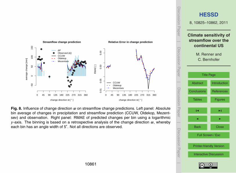
http://wwwpub.zih.tu-dresden.de/~s1748291/UWChangemapping.htm

http://wwwpub.zih.tu-dresden.de/~s1748291/UWChangemapping.htm

HESSD8, 10825–10862, 2011


continental US


Title Page



Tables Figures

J I

J I

Back Close

Full Screen / Esc



Discussion

Paper

|D

iscussionP

aper|

Discussion

Paper

|D

iscussionP

aper|

change direction ω [ ° ]

aver

age

chan

ge [m

m]

●●

●

●●

●

●

●

● ●

●

●●

●

●

●

●

●

●●

●

●

●

●●

●

●●

●●

●

●

●●●●

●

0 45 90 135 180 225 270 315 360

−50

050

100

150

Streamflow change prediction

●

∆PObserved ∆QCCUWOldekopMezentsev


RM

AE

[ ]

0 45 90 135 180 225 270 315 360

0.01

0.05

0.50

5.00

Relative Error in change prediction

CCUWOldekopMezentsev

Fig. 8. Influence of change direction ω on streamflow change predictions. Left panel: Absolutebin average of changes in precipitation and streamflow prediction (CCUW, Oldekop, Mezent-sev) and observation. Right panel: RMAE of predicted changes per bin using a logarithmicy-axis. The binning is based on a retrospective analysis of the change direction ω, wherebyeach bin has an angle width of 5◦. Not all directions are observed.

10861





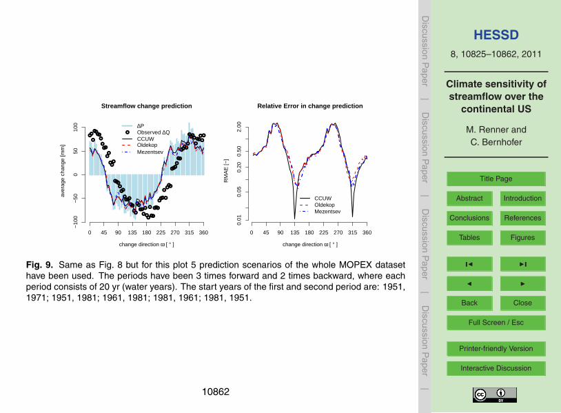
HESSD8, 10825–10862, 2011


continental US


Title Page



Tables Figures

J I

J I

Back Close

Full Screen / Esc



Discussion

Paper

|D

iscussionP

aper|

Discussion

Paper

|D

iscussionP

aper|


aver

age

chan

ge [m

m]

●●

●

●●●●

●

●●●

●●

●●●

●●●●

●●

●●●●

●●

●●

●●

●●

●

●

●●

●

●●

●●●

●●●

●

●

●●●

●●●●

●●

●●●●

●

●●●

●

●

●●●

●

●

0 45 90 135 180 225 270 315 360

−10

0−

500

5010

0

Streamflow change prediction

●

∆PObserved ∆QCCUWOldekopMezentsev


RM

AE

[−]0 45 90 135 180 225 270 315 360

0.01

0.05

0.20

0.50

2.00

Relative Error in change prediction

CCUWOldekopMezentsev

Fig. 9. Same as Fig. 8 but for this plot 5 prediction scenarios of the whole MOPEX datasethave been used. The periods have been 3 times forward and 2 times backward, where eachperiod consists of 20 yr (water years). The start years of the first and second period are: 1951,1971; 1951, 1981; 1961, 1981; 1981, 1961; 1981, 1951.

10862





Documents

Climate sensitivity of streamflow over the continental US