www.monash.edu/research/sustainability-institute

Supporting information for the National Climate Change Adaptation Research Facility (NCCARF) Coastal Settlements projects:

What would a climate-adapted settlement look like?

South East coastal adaptation (SECA) project

Climate Futures for the Southeast Australian Coast

MSI Report 12/04May 2012

Dave Griggs, Will Steffen & Tahl Kestin

Monash Sustainability Institute Building 74, Clayton Campus Monash University, Victoria 3800, Australia T: +61 3 9905 9323 E: enquiries@msi.monash.edu W: www.monash.edu/research/sustainability-institute/

Prepared by Dave Griggs & Tahl Kestin (Monash Sustainability Institute, Monash University) and Will Steffen (The ANU Climate Change Institute, Australian National University)

MSI Report 12/4, May 2012

ISBN: 978-0-9870821-2-1

Cover image: Steb Fisher

ACKNOWLEDGEMENTS This work was carried out with financial support from the Australian Government (Department of Climate Change and Energy Efficiency) and the National Climate Change Adaptation Research Facility. The views expressed herein are not necessarily the views of the Commonwealth, and the Commonwealth does not accept responsibility for any information or advice contained herein.

DISCLAIMER FOR CSIRO FIGURES CSIRO does not guarantee that the material or information it has provided is complete or accurate or without flaw of any kind, or is wholly appropriate for your particular purposes and therefore disclaims all liability for any error, loss or other consequence which may arise directly or indirectly from you relying on any information or material it has provided (in part or in whole). Any reliance on the information or material CSIRO has provided is made at the reader’s own risk.

DISCLAIMER Monash University disclaims all liability for any error, loss or consequence which may arise from relying on any information in this publication.

Table of Contents

INTRODUCTION 1

SURFACE AIR TEMPERATURE 3

Observed trends – Average surface air temperature 3Observed trends – Hot days 4Observed trends – Cold nights 5Future trends – Average surface air temperature 6Future trends – Hot days 7

RAINFALL 8

Observed trends – Annual rainfall totals 8Observed trends – Extreme rainfall 9Observed trends – Dry periods 9Future trends – Total rainfall 10Future trends – Extreme rainfall 11Future trends – Dry periods 12

SEA SURFACE TEMPERATURES 13

Observed trends – Sea surface temperatures 13Future trends – Sea surface temperatures 14

SEA LEVEL 15

Observed trends – Sea level 15Future trends – Sea level 16

COASTAL INUNDATION AND EROSION 18

BUSHFIRES 19

OTHER CLIMATE RELATED RISKS 20

SOURCE MATERIAL AND BACKGROUND READING 21

This report on climate futures is designed to serve two NCCARF projects – (i) What would a climate-adapted settlement look like?, which focuses on two communities on the Gippsland coast, and (ii) the South East Coastal Adaptation (SECA) Project, which is focussed primarily on the south coast of New South Wales.

In the analyses that follow, we have included both study areas together (referred to as the southeast Australian coast) but noted differences where they occur, differentiating the study areas as “the Gippsland coast” and “the NSW south coast”.

The section is structured around climatic variables of importance for adaptation – air temperature, rainfall (and wetness/dryness), sea surface temperature, sea level, and some aspects of storminess, such as thunderstorms and hailstorms. Where appropriate and where information is available, we consider changes in both average and extreme values of the variable. Extremes, such as heat waves and heavy rainfall events, are especially important to inform risk analysis.

For each variable we have included both the observed change in the variable up to the present and projected changes for the future. For observed change, we have focussed on the 1970–2011 trends (compared to the longer-term averages in the variable, which, for most Australian records, go back to 1900 or 1910). The last four decades encompass most of the observed trends that have been influenced by anthropogenic climate change.

The projections of future climate trends are based on a set of trajectories of future greenhouse gas emissions known as the SRES scenarios (as they were developed in the IPCC (2000) Special Report on Emission Scenarios; Figure 1). SRES provides a range of emission trajectories based on different but equally sound social, technological and policy futures.

For projections of future trends, we have focussed on two time slices – 2030 and 2070. Although 2030 will often be the most

relevant and useful timeframe for adaptation strategies, decisions on long-lived infrastructure development may also benefit from consideration of projections to 2070.

Unless otherwise specified, the projections will have the following characteristics: (i) the baseline is the average of the variable during the 1980–1999 period and is referred to as the “1990 baseline”; (ii) the 2030 projections are an average of the 2020–2039 period; (iii) the 2070 projections are an average of the 2060–2079 period; (iv) three projections are given for each time period, representing low, medium and high emission scenarios; (v) a number of climate models are used for each projection (for a given time period and emission scenario) with the results presented as percentiles (10th, 50th and 90th). More details on the projection methodology and presentation are given in the appropriate reference.

We also include some climate-related risks that are very important for adaptation but that depend on combinations or aggregations of climatic variables rather than on changes in single variables. Risks associated with coastal flooding and bushfires are good examples.

Our analyses are based on published, peer-reviewed material so far as possible. Observational data are sourced primarily from the Australian Bureau of Meteorology. Many of the projections for the future are taken from the Climate Change in Australia reports prepared by CSIRO and the Australian Bureau of Meteorology. A list of references and other supporting and background material is given at the end of the report.

FIGURE 1: SRES scenarios for future greenhouse gas emissions (coloured lines). Results presented in this report use the B1 scenario to represent low future emissions; the A1B scenario to represent medium future emissions; and either the A2 or A1FI scenarios to represent high future emissions. (Source: IPCC (2007a), Figure 3.1.)

1

Introduction

2

There is often a tension between the desire for climate futures information at fine spatial and temporal scales and the reliability of the projections at the desired scales.

This tension is manifest in several features of this section:

f There is more confidence in projections of temperature change than of rainfall change. Temperature is more directly related to the change in energy balance at the Earth’s surface, so we know the direction of change (increasing temperature) with much more confidence and can often identify well-defined ranges in the magnitude of change. Rainfall is a much more complex variable than temperature, so in many cases we don’t know the direction of rainfall change with a high degree of confidence, and the ranges in the projected changes in the magnitude of rainfall are often higher than the corresponding ranges for projected temperature changes. We have attempted to carefully describe the uncertainties around projected changes in rainfall at appropriate points in the section.

f We can say more about projected change at large spatial scales than at local or small regional scales. Thus, for many of the projections below, we treat both study areas together as a single spatial unit. In some cases, we can differentiate between the two study areas. In no cases can we carry out the analyses at any finer spatial scale than a study area as a whole. For extremes of temperature, rainfall and dryness, the analyses are reported only at the scale of southern Australia as a whole.

f In general, we have more confidence in projected changes in average values than we do in changes in extremes.

f Projections of future change in climatic variables are only meaningful at temporal scales of two decades or more. Shorter timescales are increasingly dominated by modes of natural variability than by the longer term underlying trends.

Finally, this section is based on the most up-to-date science available as of May 2012. However, climate science is continually improving so the analyses in this section should be re-visited at regular intervals as the science improves. In particular, the Fifth Assessment Report (AR5) of the Intergovernmental Panel on Climate Change (IPCC) is due to be published in 2013 (Working Group 1 – basic science) and 2014 (impacts and adaptation). Furthermore, updated climate scenarios for Australia, based on the climate model outputs assessed in the AR5, will be released on the same timeframe.

Observed Trends – Average Surface Air Temperature

FIGURE 2: Trends in temperatures over Australia over the period 1970 to 2011, plotted in degrees Celsius per decade: (a) maximum temperature; (b) minimum temperature; and (c) mean temperature (which is the average of the daily maximum and minimum temperatures). (Source: Bureau of Meteorology: http://www.bom.gov.au/climate/change/acorn-sat/.)

a) Maximum Temperature b) Minimum Temperature

c) Mean Temperature

There has been a warming trend of between 0.15 and 0.3°C every ten years in maximum temperature over the last 40 years for the southeast Australian coast, with a warming of 0.2 to 0.3°C every ten years for the Gippsland coast study area and 0.15 to 0.3°C every ten years over the NSW south coast (Figure 2a). Trends in maximum temperature tend to be slightly lower near the coast in the NSW south coast area compared to inland due to the cooling effect of the ocean, e.g., sea breezes.

There has been a warming trend of between 0.1 and 0.3°C every ten years in minimum temperature over the last 40 years for the southeast Australian coast (Figure 2b), with a warming of 0.1 to 0.2°C for the Gippsland coast study area and 0.1 to 0.3°C over the NSW south coast study area.

3

There has been an observed increase in mean (average of the daily maximum and minimum temperature) temperature of 0.1 to 0.3°C every 10 years over the last 40 years for the southeast Australian coast (Figure 2c), with the majority of the area warming between 0.1 to 0.2°C every 10 years.

Surface Air Temperature

Observed Trends – Hot Days

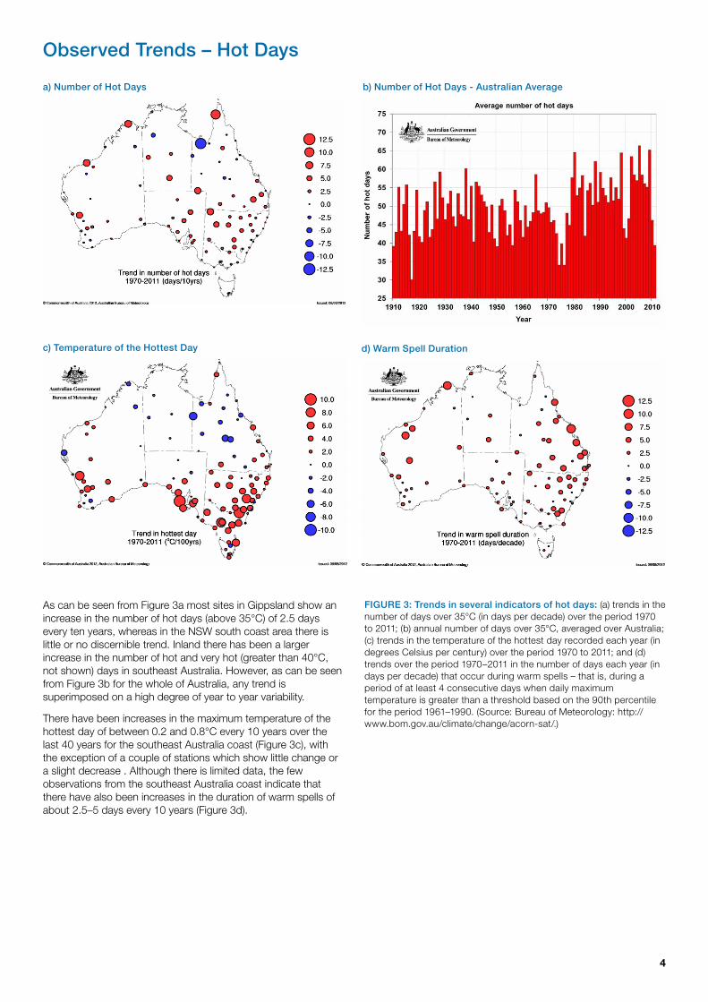
a) Number of Hot Days b) Number of Hot Days - Australian Average

c) Temperature of the Hottest Day d) Warm Spell Duration

FIGURE 3: Trends in several indicators of hot days: (a) trends in the number of days over 35°C (in days per decade) over the period 1970 to 2011; (b) annual number of days over 35°C, averaged over Australia; (c) trends in the temperature of the hottest day recorded each year (in degrees Celsius per century) over the period 1970 to 2011; and (d) trends over the period 1970–2011 in the number of days each year (in days per decade) that occur during warm spells – that is, during a period of at least 4 consecutive days when daily maximum temperature is greater than a threshold based on the 90th percentile for the period 1961–1990. (Source: Bureau of Meteorology: http://www.bom.gov.au/climate/change/acorn-sat/.)

As can be seen from Figure 3a most sites in Gippsland show an increase in the number of hot days (above 35°C) of 2.5 days every ten years, whereas in the NSW south coast area there is little or no discernible trend. Inland there has been a larger increase in the number of hot and very hot (greater than 40°C, not shown) days in southeast Australia. However, as can be seen from Figure 3b for the whole of Australia, any trend is superimposed on a high degree of year to year variability.

There have been increases in the maximum temperature of the hottest day of between 0.2 and 0.8°C every 10 years over the last 40 years for the southeast Australia coast (Figure 3c), with the exception of a couple of stations which show little change or a slight decrease . Although there is limited data, the few observations from the southeast Australia coast indicate that there have also been increases in the duration of warm spells of about 2.5–5 days every 10 years (Figure 3d).

4

Observed Trends – Cold Nights

b) Number of Cold Nights - Australian Average

c) Temperature of the Coldest Night d) Number of Frost Nights

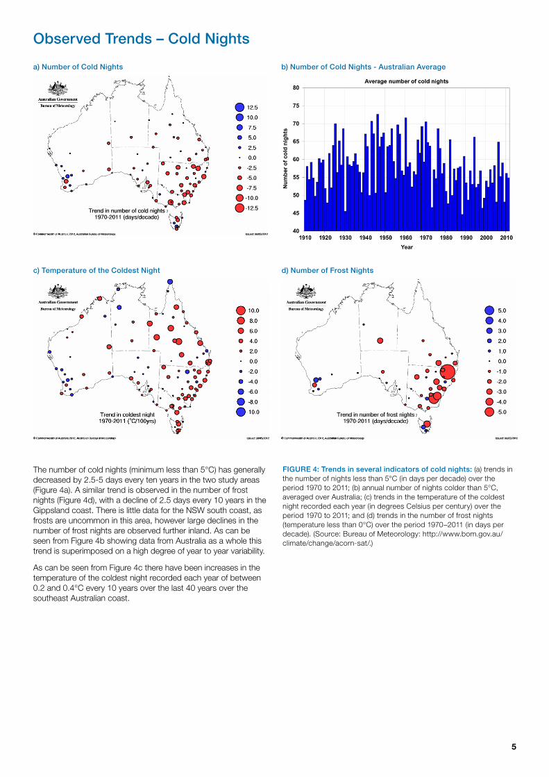
The number of cold nights (minimum less than 5°C) has generally decreased by 2.5-5 days every ten years in the two study areas (Figure 4a). A similar trend is observed in the number of frost nights (Figure 4d), with a decline of 2.5 days every 10 years in the Gippsland coast. There is little data for the NSW south coast, as frosts are uncommon in this area, however large declines in the number of frost nights are observed further inland. As can be seen from Figure 4b showing data from Australia as a whole this trend is superimposed on a high degree of year to year variability.

As can be seen from Figure 4c there have been increases in the temperature of the coldest night recorded each year of between 0.2 and 0.4°C every 10 years over the last 40 years over the southeast Australian coast.

a) Number of Cold Nights

FIGURE 4: Trends in several indicators of cold nights: (a) trends in the number of nights less than 5°C (in days per decade) over the period 1970 to 2011; (b) annual number of nights colder than 5°C, averaged over Australia; (c) trends in the temperature of the coldest night recorded each year (in degrees Celsius per century) over the period 1970 to 2011; and (d) trends in the number of frost nights (temperature less than 0°C) over the period 1970–2011 (in days per decade). (Source: Bureau of Meteorology: http://www.bom.gov.au/climate/change/acorn-sat/.)

5

Future Trends – Average Surface Air Temperature

a) 2030

b) 2070

6

FIGURE 5: Projected changes in annual average surface air temperature: (a) 2030 and (b) 2070 relative to the 1990 baseline. The 50th percentile (the mid-point of the spread of model results) provides a best estimate result. The 10th and 90th percentiles (lowest 10% and highest 10% of the spread of model results) provide a range of uncertainty. Emissions scenarios are from the IPCC Special Report on Emission Scenarios: “Low emissions” – B1 scenario; “medium emissions” – A1B scenario; and “high emissions” – A1FI scenario. (Source: CSIRO & Bureau of Meteorology (2007), Climate Change in Australia: http://www.climatechangeinaustralia.gov.au.)

By combining the low emissions scenario with the 10th percentile and the high emissions scenario with the 90th percentile a range of temperature increase for the southeast Australian coast by 2030 can be given as 0.3 to 1.5°C compared to a 1990 baseline (Figure 5a).

By combining the low emissions scenario with the 10th percentile and the high emissions scenario with the 90th percentile a range of temperature increase for the southeast Australian coast by 2070 (Figure 5b) can be given as 1 to 4°C, compared to the 1990 baseline (1980–1999 average). In this case the projected temperature increases are lower for the Gippsland coast study area (1 to 3°C) compared to the NSW south coast (1.5 to 4°C).

Future Trends – Hot Days

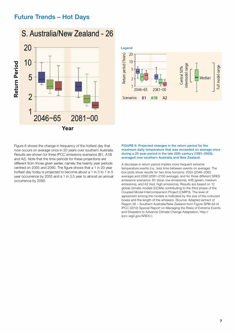
FIGURE 6: Projected changes in the return period for the maximum daily temperature that was exceeded on average once during a 20-year period in the late 20th century (1981–2000), averaged over southern Australia and New Zealand.

A decrease in return period implies more frequent extreme temperature events (i.e., less time between events on average). The box plots show results for two time horizons: 2055 (2046–2065 average) and 2090 (2081–2100 average), and for three different SRES emissions scenarios: B1 (blue, low emissions), A1B (green, medium emissions), and A2 (red, high emissions). Results are based on 12 global climate models (GCMs) contributing to the third phase of the Coupled Model Intercomparison Project (CMIP3). The level of agreement among the models is indicated by the size of the coloured boxes and the length of the whiskers. (Source: Adapted extract of Region 26 – Southern Australia/New Zealand from Figure SPM.4A of IPCC (2012) Special Report on Managing the Risks of Extreme Events and Disasters to Advance Climate Change Adaptation, http://ipcc-wg2.gov/SREX/.)

Figure 6 shows the change in frequency of the hottest day that now occurs on average once in 20 years over southern Australia. Results are shown for three IPCC emissions scenarios (B1, A1B and A2). Note that the time periods for these projections are different from those given earlier, namely the twenty year periods centred on 2055 and 2090. The figure shows that a 1 in 20 year hottest day today is projected to become about a 1 in 3 to 1 in 5 year occurrence by 2055 and a 1 in 3.5 year to almost an annual occurrence by 2090.

7

Legend

Ret

urn

Perio

d

Year

Observed Trends – Annual Rainfall Totals

b) Seasonal Trendsa) Annual Trends

SUMMER AUTUMN

WINTER SPRING

mm/10 years

c) Number of Wet Days

FIGURE 7: Trends in total rainfall: (a) annual trends in total rainfall (in mm per decade) from 1970 to 2011; (b) seasonal trends in total rainfall (in mm per decade) from 1970 to 2011; and (c) the number of wet days (days with more than 1 mm of rainfall). (Source: Bureau of Meteorology, http://www.bom.gov.au/climate/change/)

Over the past 40 years there has been a strong drying trend along the southeast Australia coast, with a decline of 30–50 mm per decade in the Gippsland coast area, and 40–60 mm per decade in the NSW south coast (Figure 7a). Mirroring the decrease in total rainfall over the past 40 years, the number of wet days has also declined in the southeast Australia coast area (Figure 7c).

8

The observed trends in rainfall show pronounced seasonality (Figure 7b), particularly for the NSW south coast. There the drying trend is especially strong in autumn, and somewhat less pronounced but still clear in summer and spring. For the Gippsland coast the drying trend is more evenly distributed throughout the year but slightly more pronounced in autumn.

Rainfall

Observed Trends – Extreme Rainfall

b) Annual Highest 1-Day Total

Over the past 40 years, extreme rainfall has declined in line with the decline in total rainfall, as shown by (i) the number of days with heavy rainfall (Figure 8a), and (ii) the highest daily precipitation each year (Figure 8b).

Both of these indicators have decreased over the 40-year period, with the reductions somewhat greater for the NSW south coast than for the Gippsland coast.

a) Number of Heavy Rain Days

FIGURE 8: Trends in indicators of extreme rainfall: (a) trends in the number of days with heavy rainfall (i.e., rainfall greater than 10 mm per day); and (b) trends in the highest daily rainfall recorded each year. (Source: Bureau of Meteorology, http://www.bom.gov.au/climate/change/.)

Observed Trends – Dry Periods

FIGURE 9: Trends (in days per century) in the maximum number of consecutive days with daily precipitation less than 1mm each year over the period 1970 to 2011. (Source: Bureau of Meteorology, http://www.bom.gov.au/climate/change/.)

While annual total rainfall has declined over southeast Australia, the number of consecutive dry days (Figure 9) has slightly decreased along the coast (shorter periods of dry weather), but has increased inland (longer periods of dry weather).

9

Future Trends – Total Rainfall

a) 2030

b) 2070

10

FIGURE 10: Projected changes in annual rainfall in: (a) 2030 and (b) 2070 relative to the 1990 baseline. The 50th percentile (the mid-point of the spread of model results) provides a best estimate result. The 10th and 90th percentiles (lowest 10% and highest 10% of the spread of model results) provide a range of uncertainty. Emissions scenarios are from the IPCC Special Report on Emission Scenarios: “Low emissions” – B1 scenario; “medium emissions” – A1B scenario; and “high emissions” – A1FI scenario. (Source: CSIRO & Bureau of Meteorology (2007), Climate Change in Australia: http://www.climatechangeinaustralia.gov.au.)

The range of uncertainty for projected rainfall change in 2030 across Australia is very large (Figure 10a). The Gippsland coast ranges from no change in rainfall to a decline of up to 10%. The NSW south coast ranges from an increase of 5% to a decline of 10%.

The range of projected rainfall changes in 2070 is high (Figure 10b), indicating a high level of uncertainty in both the future direction and magnitude of rainfall trends. For the Gippsland coast, trends in projected rainfall vary from no change to a decline of up to 40%. For the NSW south coast, trends in projected rainfall vary from an increase of 10% to a decline of up to 40%.

Future Trends – Extreme Rainfall

FIGURE 11: Projected changes in the return period for daily rainfall that was exceeded on average once during a 20-year period in the late 20th century (1981–2000), averaged over southern Australia and New Zealand.

A decrease in return period implies more frequent extreme rainfall events (i.e., less time between events on average). The box plots show results for two time horizons: 2055 (2046–2065 average) and 2090 (2081–2100 average), and for three different SRES emissions scenarios: B1 (blue, low emissions), A1B (green, medium emissions), and A2 (red, high emissions). Results are based on 14 GCMs contributing to the CMIP3. The level of agreement among the models is indicated by the size of the coloured boxes and the length of the whiskers. (Source: Adapted extract of Region 26 – Southern Australia/New Zealand from Figure SPM.4B of IPCC (2012) Special Report on Managing the Risks of Extreme Events and Disasters to Advance Climate Change Adaptation, http://ipcc-wg2.gov/SREX/)

Figure 11 shows the change in frequency of very heavy daily rainfall events that now occur on average once in 20 years over southern Australia. Results are shown for three IPCC SRES emissions scenarios (B1, A1B and A2). Note that the time periods for these projections are different from those above, namely the twenty year periods centred on 2055 and 2090. These results indicate a modest increase in extreme rainfall events over the southern Australian region. Results suggest that daily rainfall events that now occur once every 20 years will occur once every 15–17 years by 2055 and once every 9–17 years by 2090.

11

Legend

Ret

urn

Perio

d

Year

Future Trends – Dry Periods

FIGURE 12: Projected annual changes in dryness assessed from two indices: Change in annual maximum number of consecutive dry days (days with rainfall less than 1 mm) (left); and changes in soil moisture (right). Increased dryness is indicated with yellow to red colours; decreased dryness with green to blue. The figures show changes for two time horizons: 2055 (2046–2065) and 2090 (2081–2100), as compared to late 20th-century values (1980–1999), based on the SRES A2 emissions scenarios (high emissions). Grey shading indicates areas with insufficient model agreements on the sign of change; stippling indicates areas with strong model agreement. (Source: Figure SPM.5 in IPCC (2012) Special Report on Managing the Risks of Extreme Events and Disasters to Advance Climate Change Adaptation, http://ipcc-wg2.gov/SREX/.)

Projections (Figure 12) indicate an increase in the number of consecutive dry days in southeastern Australia by 2090 (2081–2100 average). However, projected decreases of soil moisture are less consistent for the same region, suggesting low confidence in future drought projections.

12

Observed Trends – Sea Surface Temperatures

FIGURE 13: Trends in annual SSTs (in degrees Celsius per decade) over the period 1970 to 2011. (Source: Bureau of Meteorology, http://www.bom.gov.au/climate/change/)

The trends in sea surface temperature (Figure 13) show a similar pattern to that for other temperature parameters, that is, a pronounced warming trend for the 1970–2011 period. Of particular importance is that the warming trend adjacent to the NSW south coast (0.20°C per decade) is higher than that for the Gippsland coast, and indeed is the highest for any of Australia’s coastal regions.

13

Sea Surface Temperatures (SSTs)

Future Trends – Sea Surface Temperatures

a) 2030

b) 2070

14

FIGURE 14: Projected changes in SSTs in: (a) 2030 and (b) 2070 relative to the 1990 baseline. The 50th percentile (the mid-point of the spread of model results) provides a best estimate result. The 10th and 90th percentiles (lowest 10% and highest 10% of the spread of model results) provide a range of uncertainty. Emissions scenarios are from the IPCC Special Report on Emission Scenarios: “Low emissions” – B1 scenario; “medium emissions” – A1B scenario; and “high emissions” – A1FI scenario. (Source: CSIRO & Bureau of Meteorology (2007), Climate Change in Australia: http://www.climatechangeinaus-tralia.gov.au.)

Increases from the 1990 baseline in SSTs of 0.3 to 2.0°C by 2030 are projected for the study areas (Figure 14a). These are equivalent to a rate of 0.075 to 0.5°C per decade. As noted previously, the observed rate of increase in SST adjacent to the NSW South Coast was 0.2°C per decade for the past 40 years. By 2070 (Figure 14b) the increase in SST is projected to range from 0.3 to 4.0°C compared to a 1990 baseline.

Observed Trends – Sea Level

a) Global sea level change a) Sea-level rise around Australia

FIGURE 15: Observed global and regional sea-level rise: (a) Global average sea-level measurements from tide gauges (blue) and satellites (red). The blue shading indicates the accuracy of the tide-gauge estimate. (b) The rate of sea-level rise around Australia as measured by coastal tide gauges (circles) and satellite observations (contours) from January 1993 to December 2011. (Source: CSIRO and BoM, State of the Climate 2012, http://www.csiro.au/State-of-the-Climate-2012.)

The average global sea level (Figure 15a) has risen by about 210 mm (21 cm or 0.21 m) from 1880 to 2011, owing both to thermal expansion from the warming of the ocean and the additional water provided by melting glaciers and ice caps. The trend from 1993 to 2011 as measured by satellites (red line in the figure) is about 3 mm per year, compared to the longer term average of 1.7 mm per year.

When compared to the global average rate of sea-level rise, there is much variation around Australia’s coasts (Figure 15b), which is crucial for understanding current and future risks associated with rising sea level. For our study areas, the observed sea-level rise from 1993 to 2011 is close to the global average of 3 mm year.

15

Sea Level

Future Trends – Sea Level

FIGURE 16: Global averaged projections of sea-level rise to 2100 relative to 1990 for several SRES scenarios. The continuous coloured lines from 1990 to 2100 indicate the central value of the projections, including the rapid ice contribution. The bars at right show the range of projections for 2100 for the various SRES scenarios. The horizontal lines/diamonds in the bars are the central values without and with the rapid ice sheet contribution. The projections are based on the IPCC Fourth Assessment Report. (Source: Church et al (2011): http://www.cmar.csiro.au/sealevel.)

Projections for global average sea-level rise for 2100, compared to the 1990 value, show a large range, from an additional 20 cm to a maximum of 80 cm (Figure 16). Much of the uncertainty is linked to the stability of the large polar ice sheets (Greenland and Antarctica), where the dynamical processes by which they can lose ice to the sea are not yet well understood. Thus, the IPCC also notes that larger values (greater than 0.8 m) cannot be ruled out. The observed sea-level rise (red line) is currently tracking near the upper limit of the envelope of IPCC projections.

16

a) 2030 b) 2070

FIGURE 17: projected departures (in mm) from the: (a) 2030, and (b) 2070, global-mean sea level from 17 SRES A1B simulations. (Source: CSIRO and Antarctic Climate and Ecosystems (ACE) CRC Sea-level rise website, http://www.cmar.csiro.au/sealevel/index.html)

Figure 17 shows the difference from the projected global average sea-level rise for areas around Australia. For our study areas, the Australian regional projections show a further increase of 2.5–5.0 cm on top of the global average sea-level rise for 2030 (left panel) and 5.0–7.5 cm for 2070 (right panel) for the southeast coasts. This means that, for planning purposes, the maximum projected sea-level rise for the study areas becomes about 20 cm in 2030 (compared to the 1990 baseline) and about 52 cm in 2070.

However, because of the uncertainties in polar ice sheet dynamics, higher values cannot be ruled out.

17

Inundation (flooding) of property and infrastructure (“high sea-level events”) and coastal erosion are the most important risks associated with a rising sea level.

The flooding events are usually associated with high tides and storm surges, with changes in sea level playing a role over longer periods of time. Some estimates have been made of the increased frequency of high sea-level events with realistic levels of sea-level rise, that is, levels that are within the IPCC range of projections for 2100 (Figure 18).

A rise of 0.5 m (50 cm) in sea level can increase the frequency of high sea-level events by a factor of 10 to 1000. These are surprisingly high multiplication factors. A multiplying factor of 100 means that a flooding event that currently occurs once in every hundred years would occur every year with a 0.5 m sea-level rise. Although there are no estimates of these multiplication factors for our study areas, the multiplication factors for Sydney and Melbourne (from 100 to 1000) suggest the potential for a very large increase in flooding events for the southeast Australian coast towards the end of this century. Using a different approach, the increase in the height of extreme storm tides (one-in-100-year events) for the eastern Victorian coast has been projected for 2030 and 2070 (Table 1).

Many coastal flooding events are associated with simultaneous high sea-level events and heavy rainfall events in the catchments inland of the coastal settlements. Little research has yet been done to connect these two phenomena and produce an overall change in risk factor for these “double whammy” coastal flooding events. For our study areas, and especially for the NSW south coast, there is a strong correlation between storm surges and heavy rainfall events as both are often caused by east coast low pressure systems. Unfortunately, climate models cannot yet simulate the behaviour of east coast lows so projections of changes in their frequency or intensity cannot yet be made. Also, no clear trends in changes in the nature of east coast lows are evident from the observational record. Indirectly, the rises in sea level over the 21st century, which are virtually certain, coupled with the projections of a modest increase in the frequency of heavy rainfall events for southern Australia (SREX) would suggest that an increased risk of these “double whammy” flooding events is more likely than not.

FIGURE 18: Estimated multiplying factor for the increase in frequency of occurrence of high sea-level events caused by a sea-level rise of 50 cm (0.5 m). (Source: Dr John Hunter, ACE CRC, http://www.acecrc.org.au/Research/Sea-Level%20Rise%20Impacts, based on Hunter (2011).)

18

AUSTRALIA

TASMANIA

FREMANTLE

DARWIN

ADELAIDE MELBOURNE

SYDNEY

HOBART

PORT HEDLAND

BUNDABERG

TOWNSVILLE

1000

100

10

LOCATIONCURRENT CLIMATE (m)

2030 2070

Low (m) Med (m) High (m) Low (m) Med (m) High (m)

Port Welshpool 1.65 1.67 1.75 1.84 1.69 1.92 2.21

Port Franklin 1.87 1.88 1.98 2.07 1.90 2.15 2.48

Port Albert 1.75 1.77 1.87 1.96 1.79 2.04 2.36

Lakes Entrance 0.98 1.00 1.09 1.17 1.02 1.25 1.56

Metung 0.59 0.61 0.70 0.78 0.63 0.86 1.16

Paynesville 0.35 0.37 0.45 0.53 0.40 0.61 0.88

TABLE 1: Projected 100-year return levels of storm tides for selected locations along the eastern Victorian coast under current climate and 2030 and 2070 low, mid and high scenarios for wind speed and sea-level rise (from McInnes et al. 2005b). (Source: CSIRO & Bureau of Meteorology, Climate Change in Australia website http://www.climat-echangeinaustralia.gov.au.)

Coastal Inundation and Erosion

The Black Saturday bushfires of 7 February 2009 in Victoria illustrate the possible connections between climate change and fire risk in areas very similar to the hinterlands of our study areas.

The four factors that form the MacArthur Forest Fire Danger Index (FFDI) are directly related to climate, and three of them – maximum temperature, relative humidity, and a drought factor – all set record values on 7 February, values that are consistent with the observed and projected trends in those variables due to climate change (Karoly 2009). The FFDI itself set record levels, ranging from 120 to 190 across sites in Victoria compared to a value of 100, which was based on the FFDI for the Black Friday fires of 1939.

Although changes in the risk of bushfires can be expected as the climate warms, observations of changed bushfire behaviour and projections of changes in the future have large uncertainties.

The IPCC Fourth Assessment Report (IPCC 2007b) analysed the climate-related factors that influence fire danger, and noted that an increase in fire danger is likely to be associated with a reduced interval between fires, increased fire intensity, faster fire spread and a decrease in fire extinguishments. In our study areas, the frequency of very high and extreme fire danger days is likely to rise 4–25% by 2020 and 15–70% by 2050 (IPCC 2007b).

19

Bushfires

Projected changes in climate extremes under different emissions scenarios generally do not strongly diverge in the coming two to three decades, but these signals are relatively small compared to natural climate variability over this time frame. Even the sign of projected changes in some climate extremes over this time frame is uncertain. For projected changes by the end of the 21st century, either model uncertainty or uncertainties associated with emissions scenarios used becomes dominant, depending on the extreme. Low-probability, high-impact changes associated with the crossing of poorly understood climate thresholds cannot be excluded, given the transient and complex nature of the climate system. Assigning ‘low confidence’ for projections of a specific extreme neither implies nor excludes the possibility of changes in this extreme.

The IPCC Special Report on Emissions Scenarios (SREX) provides estimates of global projected changes in other variables not already covered earlier in this section and also indicates where our current state of knowledge is insufficient to make projections with any degree of confidence.

Examples, generally for the end of the 21st century and relative to the climate at the end of the 20th century, include:

f “Average tropical cyclone maximum wind speed is likely to increase…It is likely that the global frequency of tropical cyclones will either decrease or remain essentially unchanged”

f “There is low confidence in projections of small spatial-scale phenomena such as tornadoes and hail…”

f “There is medium confidence that there will be a reduction in the number of extra-tropical cyclones… there is medium confidence in a projected poleward shift of extra-tropical storm tracks.” (Extra-tropical cyclones are intense low-pressure systems that occur outside tropical areas, such as over southern Australia.)

f “There is medium confidence that droughts will intensify in the 21st century in some seasons and areas…Elsewhere, there is overall low confidence because of inconsistent projections of drought changes…”

Confidence in projecting changes in the direction and magnitude of climate extremes depends on many factors, including the type of extreme, the region and season, the amount and quality of observational data, the level of understanding of the underlying processes, and the reliability of their simulation in models.

f “Projected precipitation and temperature changes imply possible changes in floods, although overall there is low confidence in projections of changes in fluvial floods…There is medium confidence…that projected increases in heavy rainfall would contribute to increases in local flooding, in some catchments or regions.”

f “There is low confidence in projections of changes in large-scale patterns of natural climate variability” [e.g., El Niño]

Two of these are of particular relevance to the study regions. Firstly, as much of the rainfall in the study regions, particularly in the autumn-winter-spring, comes from frontal systems, any southward shift in these storm tracks is likely to lead to further reductions in rainfall. The southward shift in the sub-tropical ridge and the resultant observed southward shift in storm tracks appears to be one reason why the southeast Australian coast has already observed rainfall declines.

Secondly, the low confidence in how the El Niño-Southern Oscillation (ENSO) phenomenon will be affected by climate change contributes to the uncertainty in future rainfall patterns in the study regions. Although El Niño has more profound effects on the weather of some other parts of Australia, it does also affect the weather patterns experienced by the study regions. For example, El Niño events are associated with moderate reductions in winter and spring rainfall, whereas La Niña events, the counter-parts of El Niño, are associated with moderate increases in rainfall.

20

Other Climate-Related Risks

Church, J.A., J.M. Gregory, N.J. White, S.M. Platten and J.X. Mitrovica (2011), Understanding and Projecting Sea Level Change. Oceanography (Journal of The Oceanography Society), 24(2), 130-143, doi:10.5670/oceanog.2011.33

CSIRO & Bureau of Meteorology (2007) Climate Change in Australia: http://climatechangeinaustralia.com.au/

CSIRO & Bureau of Meteorology (2012) State of the Climate 2012: http://www.csiro.au/Outcomes/Climate/Understanding/State-of-the-Climate-2012.aspx

CSIRO & Antarctic Climate & Ecosystems (ACE) CRC, Sea-level rise website: http://www.cmar.csiro.au/sealevel/

Hunter J. (2011) A simple technique for estimating an allowance for uncertain sea-level rise. Climatic Change, DOI 10.1007/s10584-011-0332-1.

IPCC (2000) Special report on emissions scenarios: A special report of Working Group III of the Intergovernmental Panel on Climate Change. [Nakicenovic, N. and Swart, R. (eds.)]. Cambridge University Press: http://www.ipcc.ch/ipccreports/sres/emission/index.php?idp=0

IPCC (2007a) Climate Change 2007: Synthesis Report. Contribution of Working Groups I, II and III to the Fourth Assessment Report of the Intergovernmental Panel on Climate Change [Core Writing Team, Pachauri, R.K and Reisinger, A. (eds.)]. IPCC, Geneva, Switzerland, 104 pp: http://www.ipcc.ch/publications_and_data/ar4/syr/en/contents.html

IPCC (2007b) Climate Change 2007: The Physical Science Basis. Contribution of Working Group I to the Fourth Assessment Report of the Intergovernmental Panel on Climate Change [Solomon, S., D. Qin, M. Manning, Z. Chen, M. Marquis, K.B. Averyt, M. Tignor and H.L. Miller (eds.)]. Cambridge University Press, Cambridge, United Kingdom and New York, NY, USA, 996 pp: http://www.ipcc.ch/publications_and_data/ar4/wg1/en/contents.html

IPCC (2012) Managing the Risks of Extreme Events and Disasters to Advance Climate Change Adaptation. A Special Report of Working Groups I and II of the Intergovernmental Panel on Climate Change [Field, C.B., V. Barros, T.F. Stocker, D. Qin, D.J. Dokken, K.L. Ebi, M.D. Mastrandrea, K.J. Mach, G.-K. Plattner, S.K. Allen, M. Tignor, and P.M. Midgley (eds.)]. Cambridge University Press, Cambridge, UK, and New York, NY, USA, 582 pp: http://ipcc-wg2.gov/SREX/

Karoly, D.J. (2009) The recent bushfires and extreme heat wave in southeast Australia. Bulletin of the Australian Meteorological and Oceanographic Society, 22: 10–13: http://www.amos.org.au/documents/item/165

21

Source Material and Background Reading