Climate-driven technical change: seasonality andthe invention of agriculture

Andrea MatrangaUniversitat Pompeu Fabra

CaSEs seminars

February 17, 2015

1 / 31

Introduction

I focus on two puzzles related to the Neolithic Revolution

I Two puzzles:I Invented independently by different groups, around the same

time.I Farmers worked more, and ate less.

I propose a new story which answers both puzzles, and test thetheory empirically.

2 / 31

Figure 1 : Locations where agriculture was invented, and their respectivedates (years Before Present).

3 / 31

Seasonality, storage, and agriculture

Agriculture and sedentism: which came first?

I Seasonality made food scarce in large areas at the same time.

I Nomads could not find food anywhere within migratory range.

I They became sedentary in order to store food.

I Being sedentary made invention of agriculture easier.

Transition is optimal for rational population at equilibrium. Nochange in preferences, fertility, technology, species composition, ortransitory shocks.

4 / 31

Figure 2 : Right panel: Seasonal locations became more common shortlybefore agriculture was invented . Left panel: binned scatterplot oftemperature seasonality and adoption; early adopters tend to be highlyseasonal, and vice versa.

5 / 31

−2

−1

01

2−

2−

10

12

100kHumans Leave Africa

60KBroad Spectrum Revolution

22kLGM

12kNeolithic

5kPeriod

0

Years Before Present

Precession x Eccentricity Axial tilt

Insolation at 65N in July

Figure 3 : Variation in orbital forcing (black, effects of axial tilt, and thecombined effect of precession and eccentricity). Data from Berger(1992). Seasonality conditions at 65◦ N (red) are indicative of those inthe rest of Northern hemisphere.

6 / 31

Related Literature

I Neolithic triggers: gradual population growth (Locay 1989),warmer climates (Diamond 1997), drier climates (Childe1935), more stable climates (Richerson et al 2001), less stableclimates (Morand 2002), intermediately stable climates(Ashraf and Michalopoulos 2014).

I Loss in consumption per capita: ‘Man’s Worst Mistake’(Diamond 1987); defense (Seabright and Rowthorn 2010);non-food goods (Weisdorf 2009), social reasons (Acemogluand Robinson 2012).

I Long-run effects of Neolithic: gradual spread (Ammerman andCavalli-Sforza 1971), earlier state formation (Wittfogel 1957),fixed capital (Diamond 1997), greater farming productivity(Harlan 1995), cultural adaptations (Alesina et al. 2013),ethno-linguistic diffusion (Bouckaert et al. 2012).

7 / 31

Rest of Presentation

I Empirics1. Climate and the Neolithic

I Seasonality and invention of agricultureI Seasonality and spread of agriculture

2. Geographic variety and agricultural adoption3. Evidence for consumption seasonality across the transition

I Conclusions and further work

8 / 31

Model: overview

Basic assumptions:

I Agents like eating more on average, and dislike eatingirregularly.

I Pure endowment economy. Endowments vary across spaceand time.

I Nomadism and storage are mutually exclusive.

I Population constant (endogenous population growth in thepaper).

9 / 31

Model predictions

I Climate seasonality should make invention of agriculture morelikely, and its spread faster.

I Presence of uncorrelated food sources should delay adoption.

I When transitioning to farming, consumption per capita shoulddrop both in the short run (loss of dispersed food sources)and in the long run (demographic effect).

I When transitioning to farming, consumption seasonalityshould decrease substantially.

All of these predictions can be tested econometrically.

10 / 31

Data sources

I Global scale:I Invention: Puruggannan and Fuller 2009. Seven sites that

invented agriculture (+17 other domestication sites), and theirdates.

I Adoption: Putterman and Trainor 2006. 160 countries andtheir dates of adoption.

I Climate: He 2010. 48 Lat × 96 Lon × 22,000 years.Reconstructed temperature and precipitation for eachtrimester. Collapsed to 44 periods of 500 years.

I Western Eurasia:I Adoption: Pinhasi et al 2005. 765 countries and their dates of

adoption.I Climate: Hijmans et al 2005. 1950-2000 averages.Climate

statistics for 10km squares.

I Others: altitude from SRTM, distance from sea, latitude,Americas dummy.

11 / 31

Construction of explanatory variables.

TempSeas = max(Temp.Warmest, 0) − max(Temp.Coldest, 0)

PrecipSeas =Precip.Wettest − Precip.Driest

MeanPrecip.

SeasIndex = max(Quantile(TempSeas),Quantile(PrecipSeas))

12 / 31

Invention of agriculture

I Was agriculture invented in highly seasonal places?

I The dataset is structured as a panel of 1036 land cells (3.75◦

squares) times 44 periods. For each cell, I have temperatureand precipitation mean, temperature and precipitationseasonality, and a dummy for whether agriculture wasinvented in that particular place and time or not.

mean sd min max

Year Adop. -4500.00 2500.43 -11500.00 0.00Temp. Seas 8.85 7.26 0.00 28.98Precip. Seas 1.35 0.67 0.16 3.58Temp. Mean 2.49 17.44 -33.98 27.64Precip. Mean 1.80 1.63 0.02 10.40Seas. Index 625.13 225.53 84.37 993.60

Observations 1036

Table 1 : Summary statistics for the adoption cross-section dataset.

13 / 31

Map of climate and invention−

45

045

−135 −90 0 90 180

Pleasant in 8k BP Seasonal in 21k BP

Independent Agri. Seasonal in 8k BP

Geographic distribution of seasonality

Figure 4 : The map shows the global distribution of seasonal locations.Pink cells were already seasonal in 21k BP. Cells that were seasonal in8,000, are in Red. Dark blue cells were hospitable in 8,000 BP. Locationsthat were not hospitable in 8,000 BP are omitted. Most of the areaswhere agriculture was invented had recently become extremely seasonal.

14 / 31

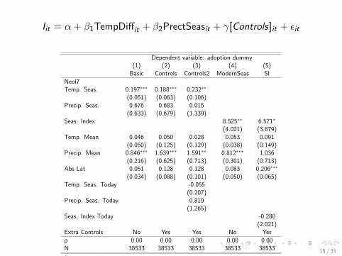
Iit = α + β1TempDiffit + β2PrectSeasit + γ[Controls]it + εit

Dependent variable: adoption dummy(1) (2) (3) (4) (5)

Basic Controls Controls2 ModernSeas SI

Neol7Temp. Seas. 0.197∗∗∗ 0.188∗∗∗ 0.232∗∗

(0.051) (0.063) (0.106)Precip. Seas. 0.676 0.683 0.015

(0.633) (0.679) (1.339)Seas. Index 8.525∗∗ 6.571∗

(4.021) (3.879)Temp. Mean 0.046 0.050 0.028 0.053 0.091

(0.050) (0.125) (0.129) (0.038) (0.149)Precip. Mean 0.846∗∗∗ 1.639∗∗∗ 1.591∗∗ 0.812∗∗∗ 1.036

(0.216) (0.625) (0.713) (0.301) (0.713)Abs Lat 0.051 0.128 0.128 0.083 0.206∗∗∗

(0.034) (0.088) (0.101) (0.050) (0.065)Temp. Seas. Today -0.055

(0.207)Precip. Seas. Today 0.819

(1.265)Seas. Index Today -0.280

(2.021)Extra Controls No Yes Yes No Yes

p 0.00 0.00 0.00 0.00 0.00N 38533 38533 38533 38533 38533

Standard errors in parentheses∗ p < 0.1, ∗∗ p < 0.05, ∗∗∗ p < 0.01

Table 2 : Duration model

15 / 31

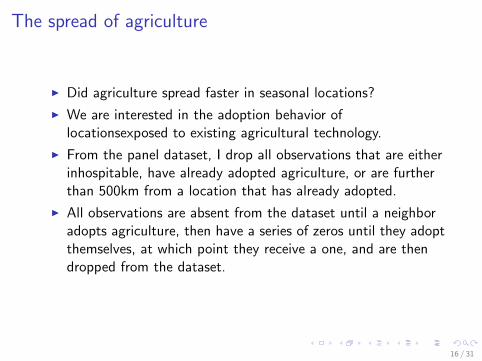
The spread of agriculture

I Did agriculture spread faster in seasonal locations?

I We are interested in the adoption behavior oflocationsexposed to existing agricultural technology.

I From the panel dataset, I drop all observations that are eitherinhospitable, have already adopted agriculture, or are furtherthan 500km from a location that has already adopted.

I All observations are absent from the dataset until a neighboradopts agriculture, then have a series of zeros until they adoptthemselves, at which point they receive a one, and are thendropped from the dataset.

16 / 31

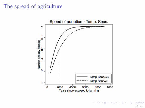
The spread of agriculture

17 / 31

The spread of agriculture

18 / 31

Ait = α + β1Tit + β2Pit + γCit + εit

Dependent variable: adoption dummy(1) (2) (3) (4) (5) (6)

Linear Linear Geog.Cluster LinearSI Logit Logit+ Geog.Cluster LogitSI

mainTemp. Seas. 0.005∗∗ 0.005∗ 0.027∗∗ 0.027∗

(0.002) (0.003) (0.011) (0.015)Precip. Seas. 0.035∗ 0.035 0.174∗ 0.174

(0.019) (0.029) (0.092) (0.144)Seas. Index 0.168∗ 0.861∗

(0.096) (0.506)Temp. Mean -0.007∗∗∗ -0.007∗ -0.007∗∗∗ -0.032∗∗∗ -0.032∗ -0.034∗∗∗

(0.002) (0.004) (0.003) (0.010) (0.017) (0.012)Precip. Mean 0.023∗∗∗ 0.023 0.017 0.113∗∗∗ 0.113 0.086

(0.008) (0.015) (0.012) (0.038) (0.071) (0.058)

Observations 1735 1735 1735 1735 1735 1735

Standard errors in parentheses∗ p < 0.1, ∗∗ p < 0.05, ∗∗∗ p < 0.01

Table 3 : Spread of agriculture. Neolithic frontier locations only.Regression of adoption dummy on climatic variables. Models 1, 2 and 3:Logit with robust s.e. Model 4, 5 and 6. Linear probability model withrobust s.e.

19 / 31

Altitude variety and early adoption

I The relationship between seasonality and the Neolithic isrobust, significant, and can be observed both at the globaland regional scale.

I I argue that the association is causal, and due to theincentives to store food.

I However, other channels are possible. Seasonal climate mayfavor proliferation of plants that are easy to cultivate (largeseeded annual grasses).

I We need a case in which seasonality is present for plants, butnot for nomads.

I I concentrate on Middle Eastern locations where wild cerealswere present, and look whether nomads were able to escape bymigrating.

20 / 31

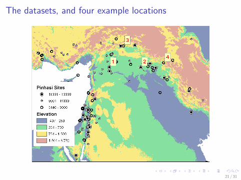
The datasets, and four example locations

21 / 31

Example: Local Areas

22 / 31

Example: Altitude Profiles

23 / 31

r(5), r(50), and date of adoption

24 / 31

Geographic correlation and early adoption

0250

500

750

1000

1250

1500

Gain

in a

ltitude r

ange (

m)

0−5km 5−50km 50−100km 100−200kmDistance from site

Adopted < 10,000 BP Adopted > 9,000 BP

Altitude variety and agricultural adoption

Figure 5 : The graph shows the altitude range that settlers could access(0-5km from site), how much extra range they could access if they werenomadic (5-50km), and how much was out of reach even for nomads(50-100km, and 100-200km). When the late adopters eventually becamesettled, they had to abandon on average 1,250m of altitude range. Theearly adopters faced a lower opportunity cost: on average they lost only1,000m.

25 / 31

Yi = α + β1r(5) + β2r(50) + γCi + εi (1)

Dependant variable: date of adoption(1) (2) (3) (4) (5)

<200km <100km Clim. Means r(200) Smooth Meas.

r(5) -0.772∗ -0.990∗∗ -0.986∗ -0.970∗

(0.414) (0.496) (0.580) (0.579)r(50) 0.414∗∗ 0.517∗∗ 0.587∗∗ 0.540∗

(0.179) (0.221) (0.267) (0.306)r(3:8) -0.858

(0.597)r(50:100) 0.500∗

(0.254)r(200) 0.111

(0.266)Temp. Seas. -161.6 -158.0 -144.5

(114.1) (116.4) (116.1)Precip. Seas. 737.9 471.2 -442.4

(4268.1) (4417.6) (4040.5)Controls No No Yes Yes Yes

Observations 129 101 101 101 101R2 0.037 0.051 0.110 0.111 0.101

Standard errors in parentheses∗ p < 0.1, ∗∗ p < 0.05, ∗∗∗ p < 0.01

Table 4 : Regression result for range of altitude within a given radius.

26 / 31

Consumption Seasonality and the Neolithic Revolution

Figure 6 : Example of Harris lines in an Inuit adult. Regular spacingreflects recurring starvation resulting in growth arrest, followed by rapidincrease in food intake and catch-up growth, forming a line of denserbone. Such a regular pattern is extremely unlikely to occur due toillnesses. Source: Lobdell(1984)

27 / 31

Conclusions

I Populations exposed to highly seasonal conditions adoptedagriculture considerably ahead of those in more stableenvironments(both greater probability of adoption, and fasterspread).

I The theory generates additional predictions on the healthoutcomes across the transition, and the local topography ofthe earliest settlements. These predictions are consistent withthe observed data.

I These findings suggest that global patterns of climaticseasonality 10,000 years ago played a dominant role indetermining where farming first appeared, what crops weredomesticated, which ethnic and linguistic groups wouldproliferate, and where the earliest cities would rise.

28 / 31

Further Work

I Predicting locations favorable to independent invention.

I Other times and periods where seasonality might beimportant.

I Storage and armies

29 / 31