Climate Change Projections of the Tasman Sea from an Ocean Eddy-resolving Model – the importance of eddies

Richard Matear, Matt Chamberlain, Chaojiao Sun, Ming Feng

CSIRO Marine and Atmospheric Research

Sun et al 2012, Chamberlain et al 2012, Matear et al., 2013 in press JGR

1

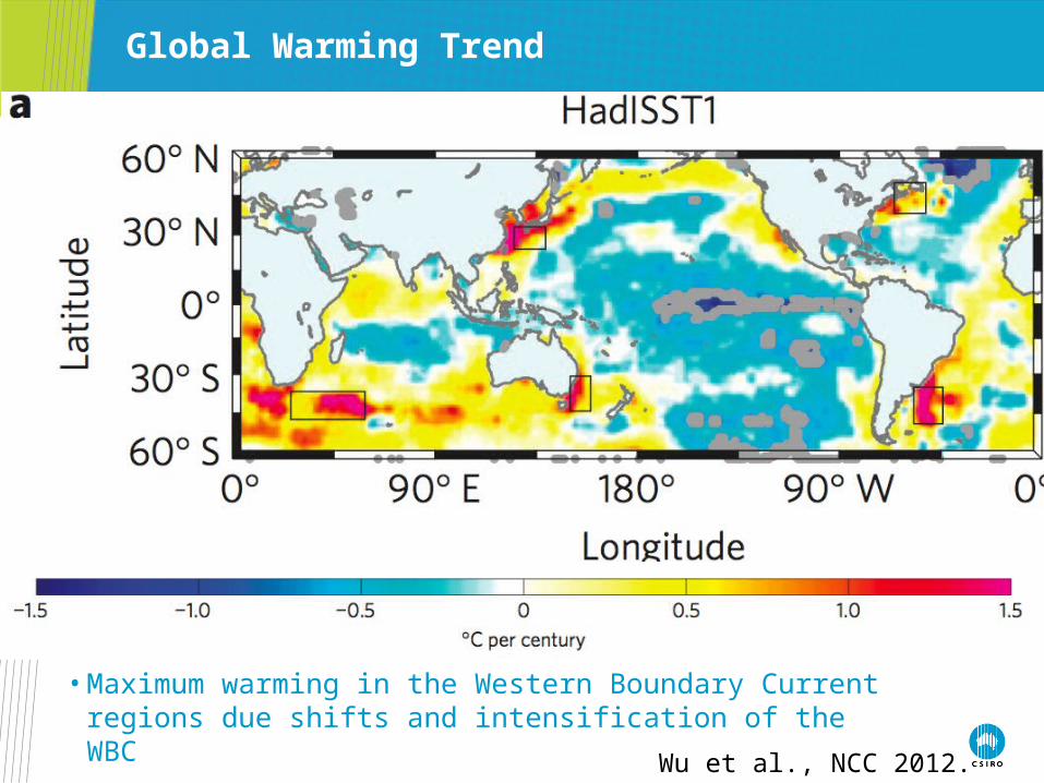
Global Warming Trend

• Maximum warming in the Western Boundary Current regions due shifts and intensification of the WBC

Wu et al., NCC 2012.

Outline

1. Why use Ocean Eddy-resolving Model?• To resolve important processes like Boundary Currents and

Eddies

2. How do we project climate change with an Ocean Eddy-resolving model• Use climate anomalies from a global climate model projection

to drive high-resolution model.

3. Consequence of resolving boundary currents and eddies• Sea surface temperature• Phytoplankton

3

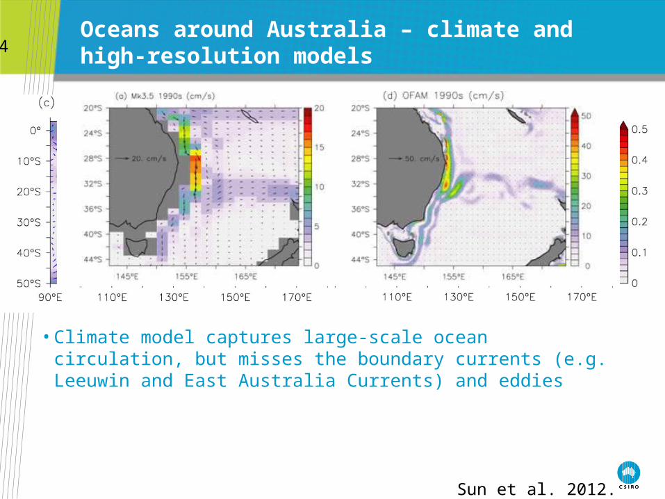
Oceans around Australia – climate and high-resolution models

• Climate model captures large-scale ocean circulation, but misses the boundary currents (e.g. Leeuwin and East Australia Currents) and eddies

Sun et al. 2012.

4

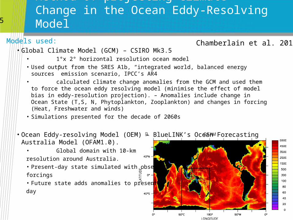
Method of projecting Climate Change in the Ocean Eddy-Resolving Model

Models used: • Global Climate Model (GCM) – CSIRO Mk3.5

• 1°x 2° horizontal resolution ocean model • Used output from the SRES A1b, “integrated world, balanced energy sources” emission

scenario, IPCC’s AR4 • calculated climate change anomalies from the GCM and used them to force

the ocean eddy resolving model (minimise the effect of model bias in eddy-resolution projection). – Anomalies include change in Ocean State (T,S, N, Phytoplankton, Zooplankton) and changes in forcing (Heat, Freshwater and winds)

• Simulations presented for the decade of 2060s

• Ocean Eddy-resolving Model (OEM) – BlueLINK’s Ocean Forecasting Australia

Model (OFAM1.0). • Global domain with 10-km

resolution around Australia.• Present-day state simulated with observed

forcings• Future state adds anomalies to present

day

Chamberlain et al. 2012

5

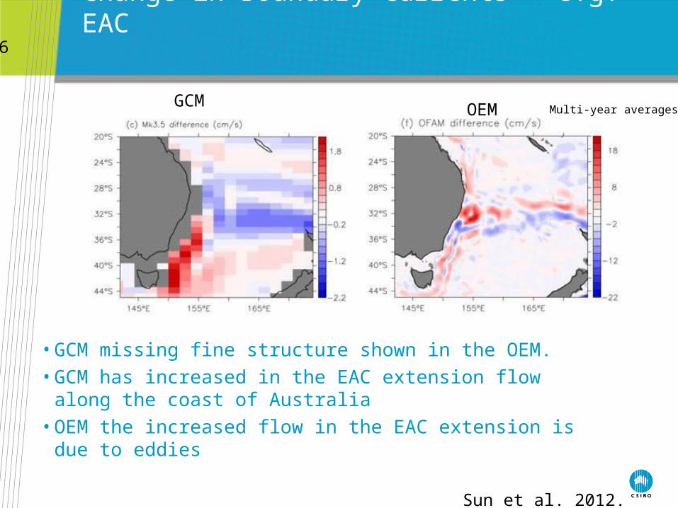
Change in Boundary Currents – e.g. EAC

Sun et al. 2012.

GCM OEM Multi-year averages

• GCM missing fine structure shown in the OEM. • GCM has increased in the EAC extension flow along the coast of

Australia• OEM the increased flow in the EAC extension is due to eddies

6

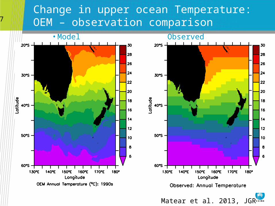
Change in upper ocean Temperature: OEM – observation comparison

Matear et al. 2013, JGR

• Model Observedmultiyear averages

7

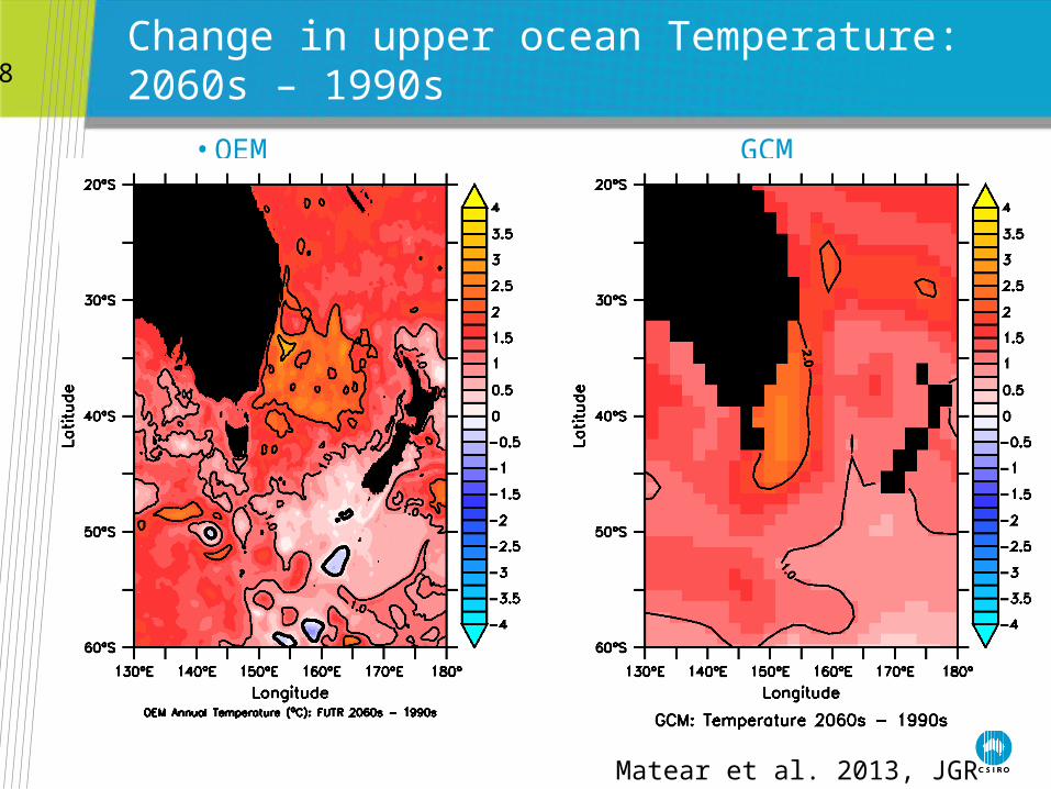
Change in upper ocean Temperature: 2060s – 1990s

Matear et al. 2013, JGR

• OEM GCM multiyear averages

8

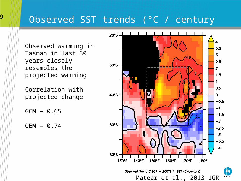
Observed SST trends (°C / century

Observed warming in Tasman in last 30 years closely resembles the projected warming

Correlation with projected change

GCM – 0.65

OEM – 0.74

Matear et al., 2013 JGR

9

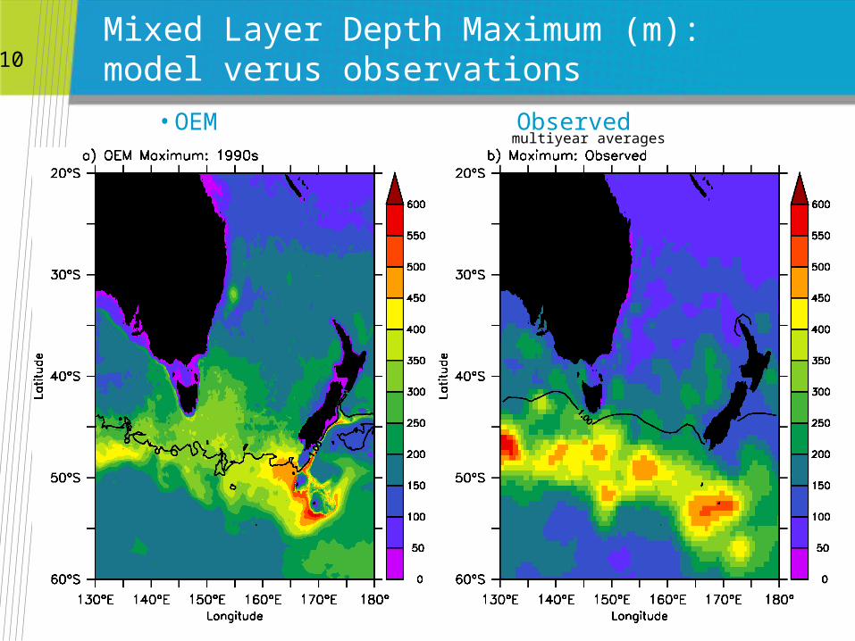
Mixed Layer Depth Maximum (m): model verus observations

Matear et al. 2013, JGR

• OEM Observed multiyear averages

10

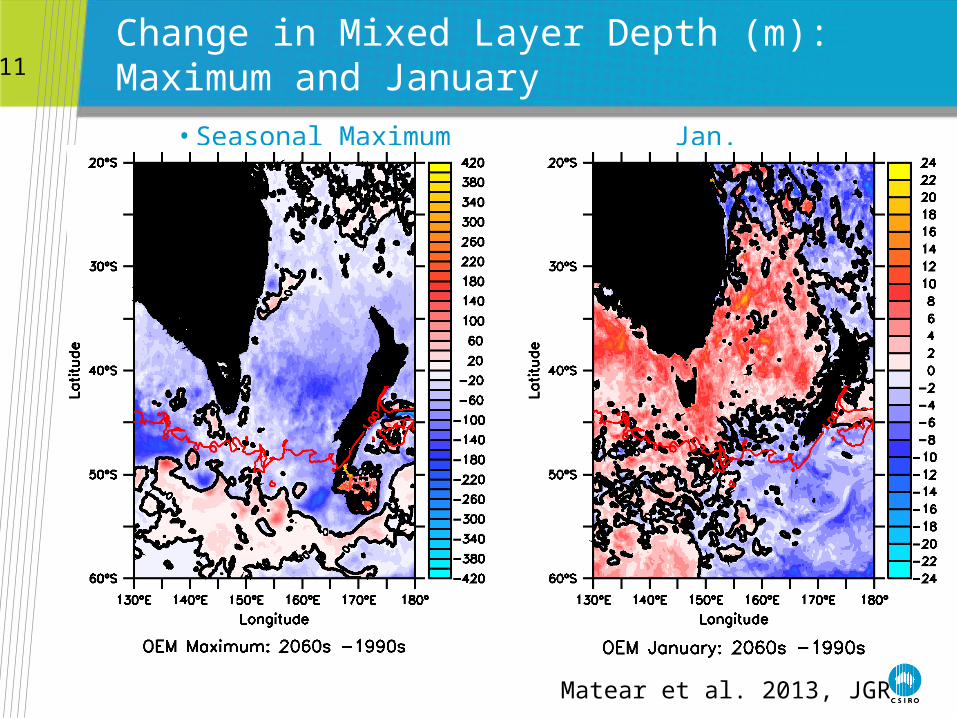
Change in Mixed Layer Depth (m): Maximum and January

Matear et al. 2013, JGR

• Seasonal Maximum Jan.

11

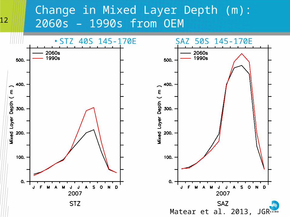
Change in Mixed Layer Depth (m): 2060s – 1990s from OEM

Matear et al. 2013, JGR

• STZ 40S 145-170E SAZ 50S 145-170E

12

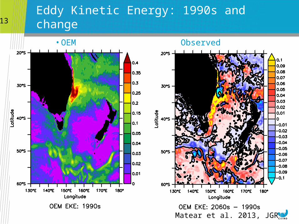
Eddy Kinetic Energy: 1990s and change

Matear et al. 2013, JGR

• OEM Observed

13

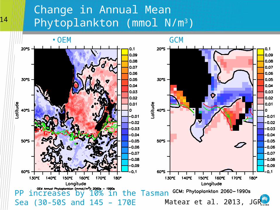
Change in Annual Mean Phytoplankton (mmol N/m3)

Matear et al. 2013, JGR

• OEM GCM

PP increases by 10% in the Tasman Sea (30-50S and 145 – 170E

14

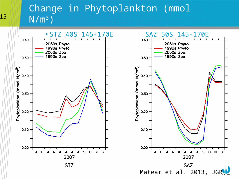
Change in Phytoplankton (mmol N/m3)

Matear et al. 2013, JGR

15

• STZ 40S 145-170E SAZ 50S 145-170E

Conclusions

Ocean Eddy-resolving Model alters the climate projection from the coarse resolution GCM by•Changing the upper ocean warming (less warming along Tasmania)•Changing the East Australian Current (EAC) response – increased EAC and increased EAC extension (more eddies)•Increasing the phytoplankton concentrations north of the Sub-Tropical Front due to increased nutrient supply from eddy-pumping.

•Primary Production in the oligotrophic Tasman Sea increases by 10% with climate change rather than declining as projected by the GCM

16

Thank you

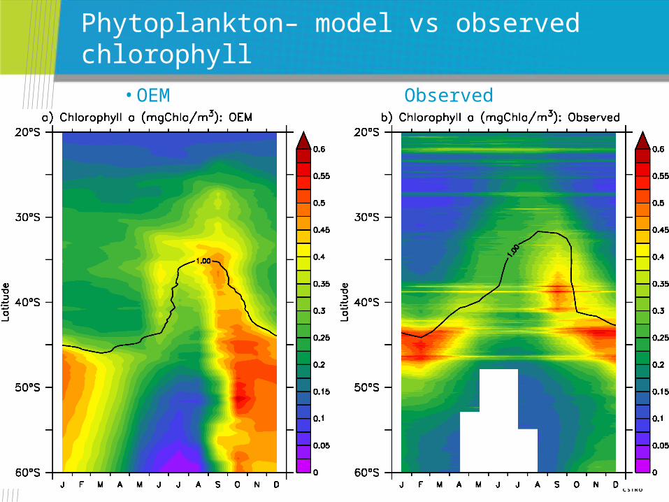
Phytoplankton– model vs observed chlorophyll

• OEM Observed

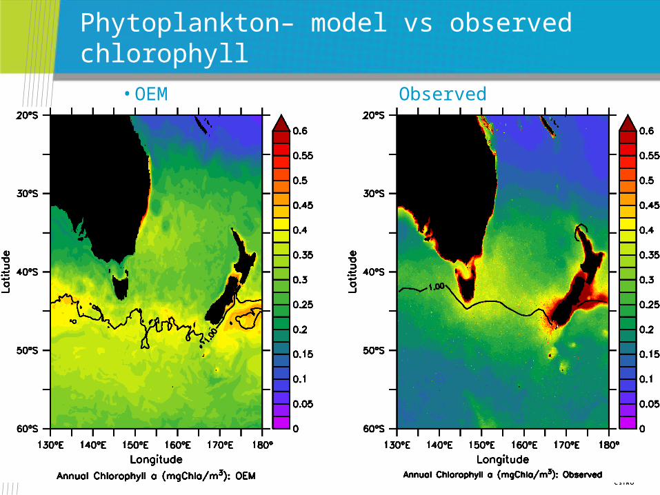
Phytoplankton– model vs observed chlorophyll

• OEM Observed

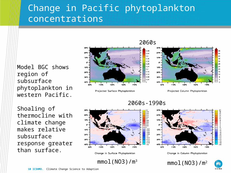
Change in Pacific phytoplankton concentrations

10 ICSHMO. Climate Change Science to Adaption

Model BGC shows region of subsurface phytoplankton in western Pacific.

Shoaling of thermocline with climate change makes relative subsurface response greater than surface.

mmol(NO3)/m3 mmol(NO3)/m2

2060s

2060s-1990s

10 ICSHMO. Climate Change Science to Adaption

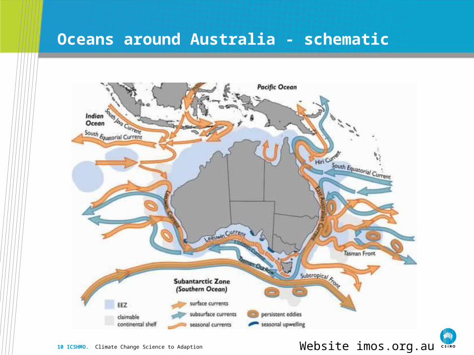
Oceans around Australia - schematic

Website imos.org.au

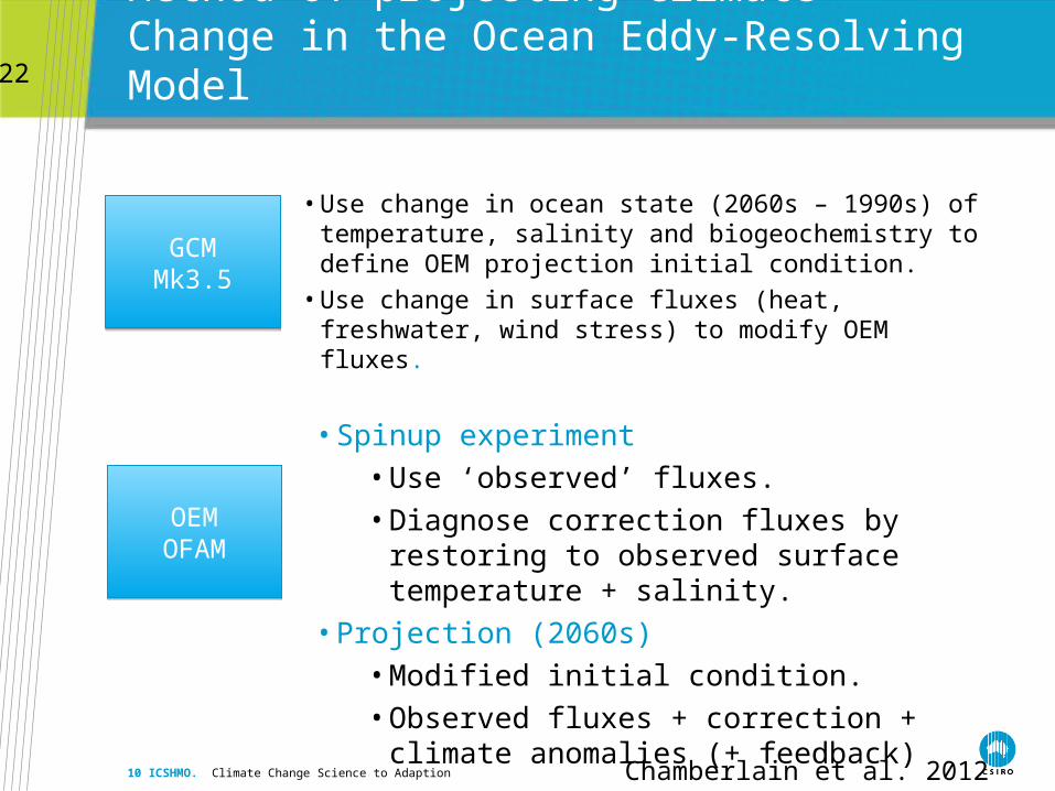
Method of projecting Climate Change in the Ocean Eddy-Resolving Model

• Use change in ocean state (2060s – 1990s) of temperature, salinity and biogeochemistry to define OEM projection initial condition.

• Use change in surface fluxes (heat, freshwater, wind stress) to modify OEM fluxes.

10 ICSHMO. Climate Change Science to Adaption

GCMMk3.5GCMMk3.5

OEMOFAMOEM

OFAM

• Spinup experiment• Use ‘observed’ fluxes.• Diagnose correction fluxes by restoring to

observed surface temperature + salinity. • Projection (2060s)

• Modified initial condition.• Observed fluxes + correction + climate

anomalies (+ feedback)

Chamberlain et al. 2012

22

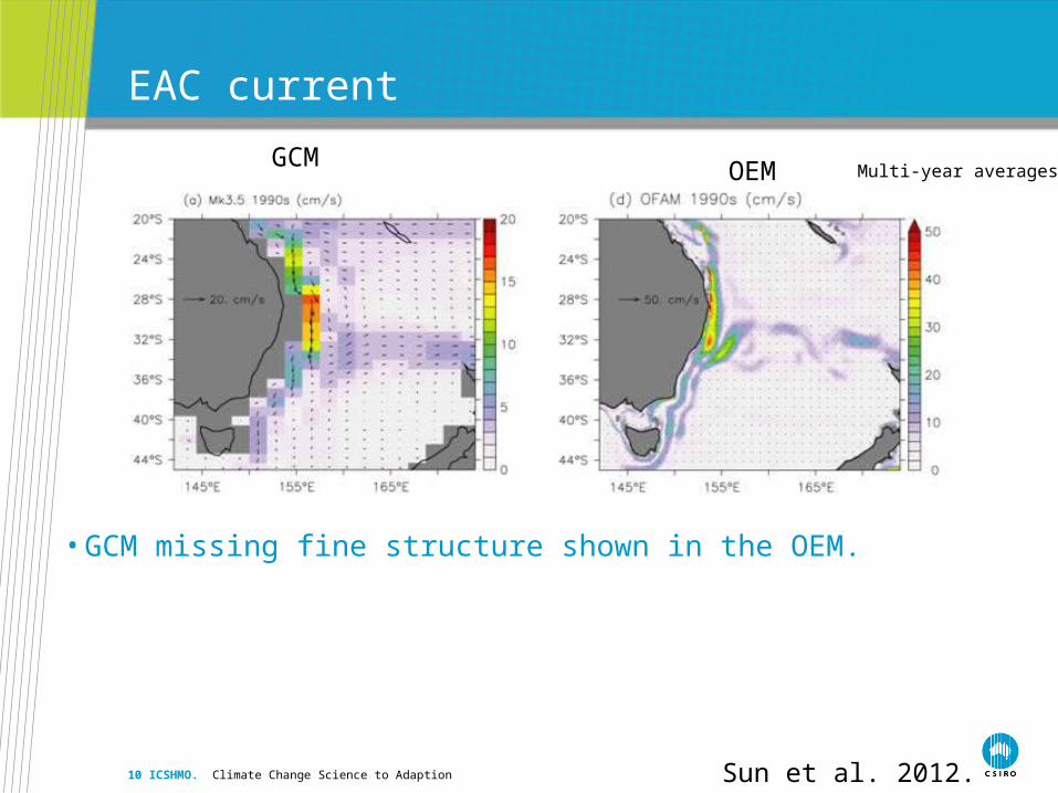
EAC current

10 ICSHMO. Climate Change Science to Adaption Sun et al. 2012.

GCM OEM Multi-year averages

• GCM missing fine structure shown in the OEM.

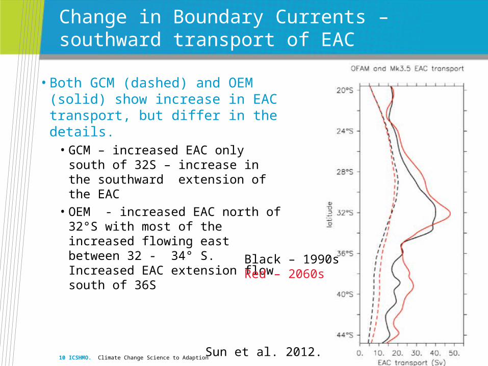
Change in Boundary Currents – southward transport of EAC

• Both GCM (dashed) and OEM (solid) show increase in EAC transport, but differ in the details.

• GCM – increased EAC only south of 32S – increase in the southward extension of the EAC

• OEM - increased EAC north of 32°S with most of the increased flowing east between 32 - 34° S. Increased EAC extension flow south of 36S

10 ICSHMO. Climate Change Science to AdaptionSun et al. 2012.

Black – 1990sRed – 2060s