Embed Size (px)
Citation preview
U.S. Department of the Interior Bureau of Reclamation August 2013
Technical Memorandum No. 1
Climate Change Analysis for the Santa Ana River Watershed Santa Ana Watershed Basin Study, California Lower Colorado Region

Mission Statements The mission of the Department of the Interior is to protect and provide access to our Nation’s natural and cultural heritage and honor our trust responsibilities to Indian Tribes and our commitments to island communities. The mission of the Bureau of Reclamation is to manage, develop, and protect water and related resources in an environmentally and economically sound manner in the interest of the American public.
i
BUREAU OF RECLAMATION Water and Environmental Resources Division (86-68200) Water Resources Planning and Operations Support Group (86-68210) Technical Services Center, Denver, Colorado Technical Memorandum No. 86-68210-2013-02
Climate Change Analysis for the Santa Ana River Watershed Santa Ana Watershed Basin Study, California Lower Colorado Region Prepared by: Kristine Blickenstaff, Hydraulic Engineer Subhrendu Gangopadhyay, Hydrologic Engineer Ian Ferguson, Hydrologic Engineer Laura Condon, Hydrologic Engineer Tom Pruitt, Civil Engineer Peer reviewed by: Marketa Elsner, Hydrologic Engineer

ii
This page intentionally left blank.
iii
Contents
Page
Executive Summary .............................................................................................. 1 1.0 Introduction ..................................................................................................... 5
1.1 Purpose, Scope, and Objective of Study .................................................... 5 1.1.1 Location and Description of Study Area ......................................... 5
1.2 Summary of Previous and Current Studies ................................................ 7 1.2.1 Historical Trends ............................................................................... 7 1.2.2 Climate Projections ........................................................................... 9 1.2.3 Hydrological Projections .................................................................. 9 1.2.4 Climate Change Impacts ................................................................. 10
1.3 Identification of Interrelated Activities .................................................... 10 1.3.1 Federal – WaterSMART ................................................................. 10 1.3.2 State – Proposition 84 and IRWM .................................................. 11 1.3.3 Local – OWOW .............................................................................. 11
2.1 Climate Projections .................................................................................. 12 2.2 Hydrology Models for the Santa Ana River Watershed .......................... 13
2.2.1 Surface Water .................................................................................. 13 2.2.2 Groundwater ................................................................................... 18
Development of Groundwater Model Inputs ...................................... 23 Historical Input Data (1990-2009) ...................................................... 23
Groundwater Elevation (ht) ........................................................... 23 Precipitation (Pt) ........................................................................... 25 Evaporative Demand (Et) .............................................................. 25 Streamflow (Qt) ............................................................................. 25 Municipal and Industrial Demand (Mt) ........................................ 27 Agricultural Demand (At) ............................................................. 27 Trans-basin Imported Water (It) ................................................... 27 Exogenous Variable (Xt) ............................................................... 27
Projected (Future) Input Data (2010-2099) ........................................ 28 Precipitation (Pt) ........................................................................... 28 Evaporative Demand (Et) .............................................................. 28 Streamflow (Qt) ............................................................................. 28 Municipal and Industrial Demand (Mt) ........................................ 28 Agricultural Demand (At) ............................................................. 29 Trans-basin Imported Water (It) ................................................... 29 Exogenous Variable (Xt) ............................................................... 29
3.0 Water Supply and Demand Projections ..................................................... 30 3.1 Water Supply ........................................................................................... 30
3.1.1 Hydroclimate Projections ................................................................ 30 Timeseries Plots .................................................................................. 30 Spatial Plots ........................................................................................ 32
3.1.2 Impacts on Runoff Annual and Seasonal Cycles ............................ 35 3.1.3 Groundwater Impacts ...................................................................... 38

iv
3.2 Water Demands ........................................................................................ 43 3.2.1 Water Demand Projections ............................................................. 43
3.3 Supply and Demand Summary ................................................................ 45 4.0 Decision Support and Impact Assessment ................................................. 46
4.1 Impacts on Recreation in Lake Elsinore .................................................. 46 4.1.1 Background ..................................................................................... 46 4.1.2 Methodology ................................................................................... 47 4.1.3 Results ............................................................................................. 47
4.2 Alpine Climate Impacts ........................................................................... 48 4.2.1 Background ..................................................................................... 48 4.2.2 Methodology ................................................................................... 49 4.2.3 Results ............................................................................................. 49
Recreation at Big Bear ........................................................................ 49 Jeffrey Pine Ecosystem ....................................................................... 51
4.3 Extreme Temperature Impacts ................................................................. 54 4.3.1 Background ..................................................................................... 54 4.3.2 Methodology ................................................................................... 54 4.3.3 Results ............................................................................................. 54
4.4 Flood Impacts ........................................................................................... 56 4.4.1 Background ..................................................................................... 56 4.4.2 Methodology ................................................................................... 58 4.4.3 Results ............................................................................................. 59
4.5 Sea Level Rise Impacts ............................................................................ 62 4.5.1 Background ..................................................................................... 62 4.5.2 Methodology ................................................................................... 62 4.5.3 Results ............................................................................................. 64
4.6 Decision Support and Impact Assessment Summary .............................. 66 5.0 Demand Management to Inform Adaptive Strategies ............................... 69
5.1 Background ............................................................................................... 69 5.2 Methods.................................................................................................... 70 5.3 Application ............................................................................................... 72
6.0 Uncertainties ................................................................................................. 75 6.1 Climate Projection Information ............................................................... 75
6.1.1 Global Climate Forcing................................................................... 75 6.1.2 Global Climate Simulations ............................................................ 76 6.1.3 Climate Projection Bias Correction ................................................ 76 6.1.4 Climate Projection Spatial Downscaling ........................................ 76
6.2 Assessing Hydrologic Impacts ................................................................. 77 6.2.1 Generating Weather Sequences Consistent with Climate Projections................................................................................................. 77 6.2.2 Natural Runoff Response ................................................................ 77 6.2.3 Hydrologic Modeling ...................................................................... 77 6.2.4 Bias and Calibration ........................................................................ 77 6.2.5 Time Resolution of the Applications .............................................. 78
7.0 References ..................................................................................................... 79
v
Figures Figure 1: SAWPA member agencies .................................................................................. 6 Figure 2: Downscaled GCM key elements figure ............................................................. 13 Figure 3: VIC macroscale hydrologic model .................................................................... 15 Figure 4: VIC routing model ............................................................................................. 16 Figure 5: Distribution of routing locations ....................................................................... 18 Figure 6: Groundwater basins and monitoring well locations .......................................... 19 Figure 7: Conceptual model of basin-scale groundwater fluctuations used in developing
the groundwater screening tool ................................................................................ 21 Figure 8: Locations for streamflow inputs ........................................................................ 26 Figure 9: Projection ensemble for six hydroclimate indicators for the site Santa Ana River
at Adams Street Gage ............................................................................................... 32 Figure 10: Spatial distribution of simulated decadal precipitation. The vertical axis
represent latitude, the horizontal axis represent longitude ....................................... 34 Figure 11: Spatial distribution of simulated decadal temperature. The vertical axis
represent latitude, the horizontal axis represent longitude ....................................... 35 Figure 12: Simulated mean annual and mean-seasonal runoff change ............................. 36 Figure 13: (a) Timeseries of observed and simulated fluctuations in monthly groundwater
elevation for the period 1990-2009; (b) scatter plot of simulated monthly change in groundwater elevation as a function of observed change groundwater elevation; (c) Timeseries of observed and simulated monthly groundwater elevation for the period 1990-2009 (zero represents mean sea level); (d) scatter plot of simulated monthly groundwater elevation as a function of observed groundwater elevation (all plots are for Orange County groundwater basin) .................................................................... 39
Figure 14: Projected groundwater elevations for Orange County for a no action scenario .......................................................................................................... 40
Figure 15: Projected groundwater elevations for Upper Santa Ana Valley for a no action scenario .................................................................................................................... 41
Figure 16: Projected groundwater elevations for San Jacinto for a no action scenario .... 42 Figure 17: Projected groundwater elevations for Elsinore for a no action scenario ......... 42 Figure 18: Population for the Santa Ana River Watershed ............................................... 43 Figure 19: Water demand by member agency (Western Municipal Water District
(WMWD); San Bernardino Valley Municipal Water District (SBVMWD); Orange County Water District (OCWD); Inland Empire Utilities Agency (IEUA); Eastern Municipal Water District (EMWD)) ........................................................................ 44
Figure 20: Santa Ana Watershed water demand calculated for this study ........................ 44 Figure 21: Lake Elsinore and VIC model grid cell used to determine data for Lake
Elsinore analysis ....................................................................................................... 47 Figure 22: Projected average annual volumes for Lake Elsinore for two future periods,
with and without EVMWD project ......................................................................... 48 Figure 23: Median percent change (from 112 climate projections) in April 1st SWE for
the grid cells containing the Bear Mountain and Snow Summit ski areas ............... 50 Figure 24: Percent change in April 1st SWE from Hayhoe et al. (2004) for areas of 2,000
to 3,000 m elevation ................................................................................................. 51 Figure 25: Fig. 4 from Lenihan et al., (2008). Percent change in total land cover for
vegetation classes by 2100 for three climate change scenarios predicted using the MC1 Dynamic Vegetation Model ............................................................................ 52
vi
Figure 26: Viability scores for Jeffery Pine currently and for three future projections for 2030 .......................................................................................................................... 53
Figure 27: Viability scores for Jeffery Pine currently and for three future projections for 2090 .......................................................................................................................... 53
Figure 28: Projected annual number of days above 95°F. Solid black line is the median and the red shading denotes the 5th and 95th percentile bounds ............................... 56
Figure 29: Station 8 Prado Dam - boxplots of 200-year flood volumes and future return periods for the median historical 200-year flood ..................................................... 59
Figure 30: Station 34 Seven Oaks Dam - boxplots of 200-year flood volumes and future return periods for the median historical 200-year flood ........................................... 60
Figure 31: Station 21 Adams Street Gage - boxplots of 200-year flood volumes and future return periods for the median historical 200-year flood ........................................... 60
Figure 32: Locations selected for OCWD analysis ........................................................... 63 Figure 33: Projections of global mean sea level rise ........................................................ 64 Figure 34: Area at risk of inundation from 100-year flood event under current conditions
(blue) and under 1400 mm sea level rise (yellow) ................................................... 65 Figure 35: AB 32 GHG Emission Reduction Targets ...................................................... 70 Figure 37: Conservation for Orange County to meet a 20% reduction in GHG emissions
by 2020 (also referred to as 20x2020) ...................................................................... 73 Figure 38: GHG emissions resulting from a 20% reduction in per capita water use every
10 years from 2020 to 2030 for Orange County ...................................................... 74 Figure 39: GHG emissions resulting from reductions in per capita water use shown in
Table 7 for Orange County....................................................................................... 74 Figure 40: Comparison of GHG emissions resulting from conservation scenarios ......... 75 Tables Table 1: Routing locations in the Santa Ana River Watershed ......................................... 17 Table 2: Streamflow locations for groundwater basins .................................................... 26 Table 3: Percent change from 1990s for annual, DJFM, and AMJJ runoff ...................... 37 Table 4: Summary of Effects of Climate Change on Supply ............................................ 45 Table 5: Summary of Water Demand for the Santa Ana River Watershed ...................... 45 Table 6: Median annual number of days above 95°F for one historical (1951-1999), and
three future (2005-2034, 2035-2064, 2055-2084) time periods ............................... 55 Table 7: Summary of 200-year flood flows (cfs) .............................................................. 61 Table 8: Summary of return periods, in years, for the median 200-year historical flood . 61 Table 9: Conservation measures required to meet AB 32 2050 target ............................. 75

vii
Acronyms and Abbreviations
°C degrees Celsius
°F degrees Fahrenheit
% percent
~ Approximately
AB 32 Assembly Bill 32
AMJJ April - July
AR4 Fourth Assessment Report
BCSD Bias Correction and Spatial Disaggregation or bias-corrected and spatially downscaled
CDF Cumulative Distribution Function
CO2e Carbon Dioxide Equivalent
CMIP Coupled Model Intercomparison Project (CMIP1, CMIP2, CMIP3, and CMIP5 are CMIP phases 1, 2, 3, and 5 respectively)
DCP Downscaled Climate Projections
DEM Digital Elevation Model
DJFM December - March
DOE U.S. Department of Energy
DWR California Department of Water Resources
EMWD Eastern Municipal Water District
EVMWD Elsinore Valley Municipal Water District
FAQs Frequently Asked Questions
GCM General Circulation Model, or Global Climate Model

viii
GHG Greenhouse Gas
IEUA Inland Empire Utilities Agency
IPCC Intergovernmental Panel on Climate Change
IRWM Integrated Regional Water Management
km kilometer
LESJWA Lake Elsinore and San Jacinto Watersheds Authority
LLNL Lawrence Livermore National Laboratory
MAF million acre-feet
MAFY million acre feet per year
MGD million gallons per day
MWDSC The Metropolitan Water District of Southern California
NCAR National Center for Atmospheric Research
OCWD Orange County Water District
OWOW One Water One Watershed
PCMDI Program for Climate Model Diagnosis and Intercomparison
PET Potential Evapotranspiration
QSA Quantification Settlement Agreement
Reclamation U.S. Department of the Interior, Bureau of Reclamation
SARP Santa Ana River Mainstem Project
SARW Santa Ana River Watershed
SAWPA Santa Ana Watershed Project Authority
SBVMWD San Bernardino Valley Municipal Water District

ix
SECURE Science and Engineering to Comprehensively Understand and Responsibly Enhance
SCAG Southern California Association of Governments
SLR Sea Level Rise
SWE Snow Water Equivalent
USGCRP U.S. Global Change Research Program
USGS U.S. Geological Survey
VIC Variable Infiltration Capacity hydrologic model
WaterSMART WaterSMART (Sustain and Manage America’s Resources for Tomorrow)
WCRP World Climate Research Programme
WMWD Western Municipal Water District
WRMS Water Resources Management System

x

Climate Change Analysis for the Santa Ana River Watershed – California Santa Ana Watershed Basin Study
1
Executive Summary The Santa Ana Watershed Basin Study (Basin Study) is a collaborative effort by the Santa Ana Watershed Project Authority (SAWPA) and the Bureau of Reclamation (Reclamation), authorized under the Sustain and Manage America's Resources for Tomorrow SECURE Water Act (Title IX, Subtitle F of Public Law 111-11). The study began in 2011 and was completed in the spring of 2013. The Basin Study complements SAWPA’s Integrated Regional Water Management (IRWM) planning process, also known as the “One Water One Watershed” (OWOW) Plan, and refines the watershed’s water projections, and identifies potential adaptation strategies, in light of projected effects of climate change. This climate change analysis for the Santa Ana River Watershed (SARW) is a contributing section to the Basin Study. This report explains the methods used to develop an analysis of potential implications of the changing climate, and how those implications might affect issues of importance to the Santa Ana River Watershed. Chapter 1 provides an introduction to the project and the study area, along with a summary of relevant previous studies. The development of climate projections and hydrology models used can be found in Chapter 2. Chapter 3 provides projections for water supply and demand in the SARW. An impact analysis was conducted focusing on key areas of importance to the SARW, the results of which can be found in Chapter 4. A tool to evaluate demand management is presented in Chapter 5, along with a case study of potential adaptation strategies. Chapter 6 addresses uncertainties in climate change analysis. In light of climate change, prolonged drought conditions, growth, and population projections, a strong concern exists to ensure there will be adequate water supplies to meet future water demand. The findings of this Basin Study will be used to update the OWOW Plan, evaluate the implications of climate change, assess increased energy demand, and ensure that future water quality and supply needs are met. Goals of the study include: incorporating existing regional and local planning studies within the watershed; sustaining the innovative “bottom up” approach to regional water resources management planning; ensuring an integrated, collaborative approach; using science and technology to assess climate change and greenhouse emissions effects; facilitating watershed adaptation planning; and expanding outreach to all major water uses and stakeholders. Future water supply was analyzed for the Santa Ana River Watershed using the Variable Infiltration Capacity (VIC) hydrologic model (Liang et al., 1994; Liang et al., 1996; Nijssen et al., 1997) to project streamflow using 112 different projections of future climate. Projected climate variables, including daily precipitation, minimum temperature, maximum temperature, and wind speed,
Climate Change Analysis for the Santa Ana River Watershed – California Santa Ana Watershed Basin Study
2
came from the Bias Corrected and Spatially Downscaled Coupled Model Intercomparison Project Phase 3 (BCSD-CMIP3) archive. Historical VIC model simulations over the period 1950-1999 were conducted using historical meteorological forcings (factors affecting the climate of the earth that drive or “force” the climate to change) developed by Maurer et al., (2002), and subsequent extensions. The VIC hydrologic model solves the water balance for each of a series of 1/8° by 1/8° (~12km x 12 km) grid cells, which represent the watershed. Daily climate projections span the time period January 1, 1950 to December 31, 2099 and exist for each grid cell. Grid based outputs of daily runoff and baseflow generated by the VIC hydrologic model are routed to select sites throughout the watershed to produce daily streamflow projections. Through coordination with SAWPA and local water agencies, 36 key locations in the basin were determined, so that sub-basins could be delineated. Change factors were developed by calculating decade mean (reference decade – 1990s; three future decades – 2020s, 2050s, and 2070s) total precipitation and temperature, then calculating percent change, and finally calculating the median change for all the 112 projections. Final products include data sets at key locations for precipitation, temperature, evapotranspiration, April 1st Snow Water Equivalent (SWE), and streamflow. These data sets were used to answer frequently asked questions regarding impacts of climate change on the Santa Ana River Watershed. The questions and key findings can be found below. Will surface water supply decrease?
• Annual surface water is likely to decrease over future periods. • Precipitation shows somewhat long term decreasing trends. • Temperature will increase, which is likely to cause increased water
demand and reservoir evaporation. • April 1st SWE will decrease.
Will groundwater availability be reduced?
• Groundwater currently provides approximately 54% of total water supply in an average year, and groundwater use is projected to increase over the next 20 years.
• Projected decreases in precipitation and increases in temperature will decrease natural recharge throughout the basin. • Management actions such as reducing municipal and industrial
water demands or increasing trans-basin water imports and recharge will be required in order to maintain current groundwater levels.
• A basin-scale groundwater screening tool was developed to facilitate analysis of basin-scale effects of conservation, increasing imported supply, changing agricultural land use, and other factors on basin-scale groundwater conditions.
Climate Change Analysis for the Santa Ana River Watershed – California Santa Ana Watershed Basin Study
3
Is Lake Elsinore in danger of drying up?
• Lake Elsinore has less than a 10% chance of drying up (2000- 2099). • In the 2000-2049 period, Lake Elsinore has a greater than 75% chance of meeting the minimum elevation goal of 1,240 ft. • In the future period 2050-2099, Lake Elsinore has less than a 50% chance of meeting the minimum elevation goal of 1,240 ft. • There is less than a 25% chance that Lake Elsinore will drop below low lake levels (1,234 ft) in either period. • The Elsinore Valley Municipal Water District (EVMWD) project does aid in stabilizing lake levels; however, for the period 2050- 2099 additional measures will likely be required to help meet the minimum elevation goal of 1,240 ft.
Will the region continue to support an alpine climate and how will the Jeffrey Pine ecosystem be impacted?
• Warmer temperatures will likely cause Jeffrey pines to move to higher elevations and may decrease their total habitat. • Forest health may also be influenced by changes in the magnitude
and frequency of wildfires or infestations. • Alpine ecosystems are vulnerable to climate change because they have little ability to expand to higher elevations. • Across the State it is projected that alpine forests will decrease in area by 50-70% by 2100.
Will skiing at Big Bear Mountain Resorts be sustained?
• Simulations indicate significant decreases in April 1st snowpack that amplify throughout the 21st century. • Warmer temperatures will also result in a delayed onset and shortened ski season. • Lower elevations are most vulnerable to increasing temperatures. • Both Big Bear Mountain Resorts lie below 3,000 m and are projected to experience declining snowpack that could exceed 70% by 2070.
How many additional days over 95°F are expected in Anaheim, Riverside and Big Bear City?
• All the climate projections demonstrate clear increasing temperature trends. • Increasing temperatures will result in a greater number of days above 95°F in the future.
Climate Change Analysis for the Santa Ana River Watershed – California Santa Ana Watershed Basin Study
4
• The number of days above 95°F gets progressively larger for all cities advancing into the future. • By 2070 it is projected that the number of days above 95°F will quadruple in Anaheim (4 to 16 days) and nearly double in Riverside (43 to 82 days). The number of days above 95°F at Big Bear City is projected to increase from 0 days historically to 4 days in 2070.
Will floods become more severe and threaten flood infrastructure?
• Simulations indicate a significant increase in flow for 200-year storm events in the future.
• The likelihood of experiencing what was historically a 200-year event will nearly double (i.e. the 200-year historical event is likely to be closer to a 100-year event in the future). • Findings indicate an increased risk of severe floods in the future, though there is large variability between climate simulations.
How will climate change and sea level rise affect coastal communities and beaches?
• Climate change will contribute to global sea level rise (SLR) through melting of glaciers and ice caps and thermal expansion of ocean waters, both of which increase the volume of water in the oceans. • Regional SLR may be higher or lower than global SLR due to effects of regional ocean and atmospheric circulation. • Average sea levels along the Southern California coast are
projected to rise by 5-24 inches by 2050 and 16-66 inches by 2100.
• SLR is likely to inundate beaches and coastal wetlands and may increase coastal erosion. Effects on local beaches depend on changes in coastal ocean currents and storm intensity, which are highly uncertain at this time. • SLR will increase the area at risk of inundation due to a 100-year flood event. • Existing barriers are sufficient to deter seawater intrusion at Talbert and Alamitos gaps under a 3-foot rise in sea levels. However, operation of barriers under SLR may be constrained by shallow groundwater concerns.
As climate science continues to evolve, periodic reanalysis and evaluation will be needed to inform the decision-making process.
Climate Change Analysis for the Santa Ana River Watershed – California Santa Ana Watershed Basin Study
5
1.0 Introduction
1.1 Purpose, Scope, and Objective of Study
The Santa Ana Watershed Basin Study (Basin Study) is a collaborative effort by the Santa Ana Watershed Project Authority (SAWPA) and the Bureau of Reclamation (Reclamation), authorized under the Sustain and Manage America's Resources for Tomorrow SECURE Water Act (Title IX, Subtitle F of Public Law 111-11). The study began in 2011 and was completed in the spring of 2013. The Basin Study complements SAWPA’s Integrated Regional Water Management (IRWM) planning process, also known as their “One Water One Watershed” (OWOW) Plan, and refines the watershed’s water projections, and identifies potential adaptation strategies, in light of projected effects of climate change. This climate change analysis for the Santa Ana River Watershed is a contributing section to the Basin Study. SAWPA is a joint powers authority that represents five major water resource agencies. SAWPA’s area includes over 350 water, wastewater and groundwater management, flood control, environmental, and other nongovernmental organizations. These entities work together collaboratively and focus on the region’s OWOW Plan. In light of climate change, prolonged drought conditions, growth, and population projections, a strong concern exists to ensure there will be adequate water supplies to meet future water demand. The findings of this Basin Study will be used to update the OWOW Plan, evaluate the implications of climate change, and ensure that future water quality and supply needs are met. Goals of the study include: incorporating existing regional and local planning studies within the watershed; sustaining the innovative “bottom up” approach to regional water resources management planning; ensuring an integrated, collaborative approach; using science and technology to assess climate change and greenhouse emissions affects; facilitating watershed adaptation planning; and expanding outreach to all major water uses and stakeholders.
1.1.1 Location and Description of Study Area The Santa Ana River Watershed (also referred to as SARW, or ‘Watershed’) is home to over 6 million people, within an area of 2,650 square miles in southern California. The regional population is projected to grow to almost ten million within the next 50 years (U.S. Census Bureau, 2010). The watershed includes much of Orange County, the northwestern corner of Riverside County, the southwestern corner of the San Bernardino County, and small portions of Las Angeles County. The watershed is bounded on the south by the Santa Margarita watershed, on the east by the Salton Sea and Southern Mojave watersheds, and on the northwest by the Mojave and San Gabriel watersheds. SAWPA has five member agencies: Eastern Municipal Water District (EMWD), Inland Empire
Climate Change Analysis for the Santa Ana River Watershed – California Santa Ana Watershed Basin Study
6
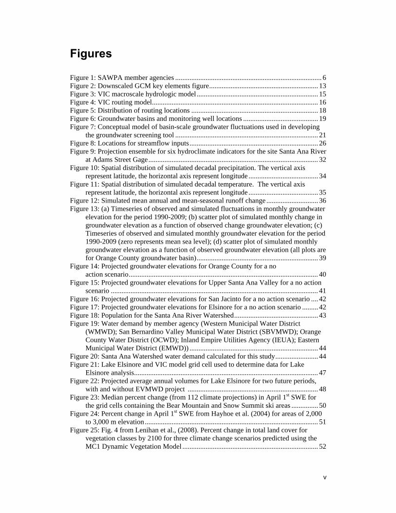
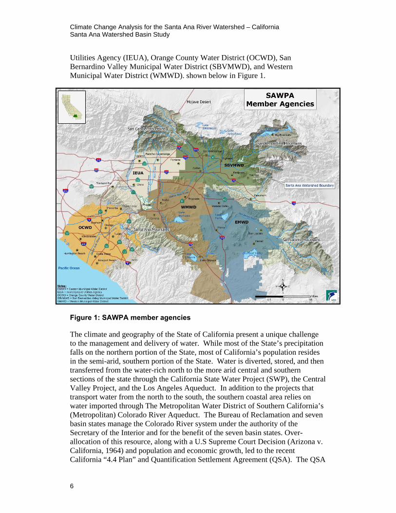
Utilities Agency (IEUA), Orange County Water District (OCWD), San Bernardino Valley Municipal Water District (SBVMWD), and Western Municipal Water District (WMWD). shown below in Figure 1.
Figure 1: SAWPA member agencies The climate and geography of the State of California present a unique challenge to the management and delivery of water. While most of the State’s precipitation falls on the northern portion of the State, most of California’s population resides in the semi-arid, southern portion of the State. Water is diverted, stored, and then transferred from the water-rich north to the more arid central and southern sections of the state through the California State Water Project (SWP), the Central Valley Project, and the Los Angeles Aqueduct. In addition to the projects that transport water from the north to the south, the southern coastal area relies on water imported through The Metropolitan Water District of Southern California’s (Metropolitan) Colorado River Aqueduct. The Bureau of Reclamation and seven basin states manage the Colorado River system under the authority of the Secretary of the Interior and for the benefit of the seven basin states. Over-allocation of this resource, along with a U.S Supreme Court Decision (Arizona v. California, 1964) and population and economic growth, led to the recent California “4.4 Plan” and Quantification Settlement Agreement (QSA). The QSA

Climate Change Analysis for the Santa Ana River Watershed – California Santa Ana Watershed Basin Study
7
limits California’s share of the Colorado River water supply to 4.4 million acre-feet (MAF). As a result of these actions, Metropolitan’s supply from the Colorado River was significantly reduced, especially during extended dry periods. In the past, a buffer supply was developed by constructing new facilities, such as dams and/or aqueducts, to provide water supply for future growth. Today, the gap between supply and demand has closed and increasing emphasis is placed on conservation and development of local supplies. Building new facilities is costly and such projects face strict environmental review before they can be approved. This has caused California to seek more creative and sustainable solutions to water resource management.
1.2 Summary of Previous and Current Studies
A large body of research has been conducted over the past ten or more years on climate change and its potential impacts on the western United States. Most of this research has focused on large scale implications (for example, over the western United States), while providing limited regional scale information. The following section summarizes research that is relevant to the Watershed, and shows that although these results are applicable, additional research was required, through this Basin Study, to evaluate smaller scale, site specific, climate change impacts. For additional information on previous and current climate change studies, not directly related to the Watershed, please see Reclamation’s Literature Synthesis on Climate Change Implications for Water and Environmental Resources (http://www.usbr.gov/research/docs/climatechangelitsynthesis.pdf).
1.2.1 Historical Trends California’s historical temperature has increased by about 1.7°F over the past 116 years (Moser et al., 2012), while showing declines in spring snowpack and a shift to earlier spring runoff (Knowles et al., 2007; Regonda et al., 2005; Peterson et al., 2008; Stewart et al., 2009). It is difficult to distinguish long-term climate change from natural climate variability, although many studies have tried to distinguish between the two (Bonfils et al., 2007; Cayan et al., 2001; Gershunov et al., 2009). It is likely that the historical temperature trends are due to a combination of anthropogenic climate change and natural climate variability (Reclamation, 2011k). A study by Gershunov et al., (2012) shows that generally, there is a positive trend (1950-2010) in heat wave activity over the entire California region that is expressed most strongly and clearly in nighttime rather than daytime temperature extremes. This trend in nighttime heat wave activity has intensified markedly since the 1980s and especially since 2000. The two most recent nighttime heat waves were also strongly expressed in extreme daytime temperatures. Circulations associated with great regional heat waves advect hot air into the region. This air can be dry or moist, depending on whether a moisture source is available, causing heat waves to be expressed preferentially during day or night.
Climate Change Analysis for the Santa Ana River Watershed – California Santa Ana Watershed Basin Study
8
A remote moisture source centered within a marine region west of Baja California has been increasing in prominence because of gradual sea surface warming and a related increase in atmospheric humidity. Adding to the very strong synoptic dynamics during the 2006 heat wave were a prolonged stream of moisture from this southwestern source, and despite the heightened humidity, an environment in which afternoon convection was suppressed, keeping cloudiness low and daytime temperatures high. Vermeera and Rahmstorf (2009) suggest a simple relationship linking global sea-level variations to temperature. This relationship is tested on synthetic data from a global climate model for the past millennium and the next century. When applied to observed data of sea level and temperature for 1880–2000, and taking into account known anthropogenic hydrologic contributions to sea level, the correlation explains 98% of the variance. Trends in historical precipitation are more sporadic making it difficult to attribute them to climate change (Hoerling et al., 2010). A series of regression analyses, conducted by Dettinger and Cayan (1995), indicate that runoff timing responds equally to the observed decadal-scale trends in winter temperature and interannual temperature variations of the same magnitude, suggesting that the trend in temperature is sufficient to explain the increasingly early runoff. However, this trend is not immediately distinguishable from natural atmospheric variability. A well‐documented shift towards earlier runoff can be attributed, in part, to more precipitation falling as rain instead of snow (Regonda et al., 2005; Pierce et al., 2008; Das et al., 2009; Hidalgo et al., 2009; Lindquist et al., 2009). Knowles et al., (2007) showed a regional trend during the period 1949–2001 toward smaller ratios of winter‐total snowfall water equivalent (SWE) to winter‐total precipitation, with the most pronounced reductions occurring in the Sierra Nevada and the Pacific Northwest, with more varied changes (but still predominantly reductions) in the Rockies. The trends in this ratio correspond to shifts toward less SWE rather than to changes in overall precipitation, except in the Southern Rockies, where both snowfall and precipitation have increased. The trends toward reduced SWE are a response to warming across the region, with the most significant reductions occurring where winter‐average wet‐day minimum temperature changes have been less than +3°C over the course of the study period. The observed trends in hydroclimatology over the western United States will likely have significant impacts on water resources planning and management. There have been preliminary efforts by agencies managing California’s water resources to incorporate climate change research into their planning and management tools, including preliminary modeling studies of potential impacts of climate change to operations of the State Water Project and Central Valley Project, Delta water quality and water levels, flood forecasting and evapotranspiration rates (Anderson et al., 2008).
Climate Change Analysis for the Santa Ana River Watershed – California Santa Ana Watershed Basin Study
9
1.2.2 Climate Projections The Intergovernmental Panel on Climate Change (IPCC) projections of future climate have been utilized in assessing climate over California. Projections indicate the rate of increase in global mean annual temperature nearly doubles before 2100, and that increases in summer temperatures are greater than winter (IPCC, 2007). There is less confidence in projections of future precipitation than temperature (Reclamation, 2011). However, precipitation projections show less snowfall and more rainfall, less snowpack development and earlier runoff, more intense and heavy rainfall interspersed with longer dry periods (Congressional Budget Office, 2009; Lundquist et al., 2009; Moser et al., 2009; Rauscher et a l2008; Maurer et al.,2007).
1.2.3 Hydrological Projections The changing climate will likely result in lower stream flow, lower reservoir storage, and decreased water supply deliveries and reliability later in the 21st century throughout California (Vicuna and Dracup, 2007). Drought in the Southwest may no longer be driven by precipitation, but rather by temperature (Hoerling and Eischeid, 2007). Two hydrologic impacts, in which there is high confidence, are increasing winter streamflow and decreasing late spring and summer flow (Maurer, 2007). There is also high confidence in reduced snowpack at the end of winter, and earlier arrival of the annual peak flow volume, which has important implications for California’s water management. The shift to earlier peak streamflow timing, and the decline in end-of-winter snow pack, results in more extreme impacts under higher emissions scenarios in all cases. This indicates that future emissions scenarios play a significant role in the degree of impacts to water resources in California. The potential effects of climate change on the hydrology and water resources of the Sacramento–San Joaquin River Basin were evaluated by Van Rheenen et al., (2004) using an ensemble of climate projections generated by the U.S. Department of Energy and National Center for Atmospheric Research Parallel Climate Model (DOE/NCAR PCM). From these global simulations, transient monthly temperature and precipitation sequences were statistically downscaled to produce continuous daily hydrologic model forcings, which drove a macro-scale hydrology model (VIC) of the Sacramento–San Joaquin River Basins at a 1/8° spatial resolution, and produced daily streamflow sequences for each climate projection. Each streamflow scenario was used in a water resources system model that simulated current and predicted future performance of the system. Results from the water resources system model indicated that achieving and maintaining status quo system performance in the future would be nearly impossible, given the altered hydrologic projections.
Climate Change Analysis for the Santa Ana River Watershed – California Santa Ana Watershed Basin Study
10
1.2.4 Climate Change Impacts With respect to management, a number of studies have investigated the implications of climate change on water management in the region, suggesting management of reservoir systems will become more challenging (Vicuna and Dracup, 2007). The impacts are expected to be expensive, but not catastrophic for California (Harou et al., 2010). Subtle changes in hydrology due to climate change can alter wetlands, resulting in a positive biotic feedback, contributing methane and carbon dioxide to the atmosphere (Burkett and Kusler, 2007). Policy options for minimizing the adverse impacts of climate change on wetland ecosystems include the reduction of current anthropogenic stresses, allowing for inland migration of coastal wetlands as sea-level rises, active management to preserve wetland hydrology, and a wide range of other management and restoration options. Ficke et al. (2007) summarizes the general effects of climate change on freshwater systems to be increased water temperatures, decreased dissolved oxygen levels, and the increased toxicity of pollutants. Altered hydrologic regimes and increased groundwater temperatures could affect the quality of fish habitat. Eutrophication may be exacerbated and stratification will likely become more pronounced. Model predictions indicate that global climate change will continue even if greenhouse gas emissions decrease or cease. Therefore, proactive management strategies such as removing other stressors from natural systems will be necessary to sustain our freshwater fisheries. Projected temperature and carbon dioxide increases may extend growing seasons, stimulate weed growth, increase pests, and may impact pollination (Baldocchi and Wong 2006). Stream temperatures in many areas are increasing due to increases in air temperature and reduced summer flows that make streams more sensitive to warmer air temperatures (Haak et al., 2010).
1.3 Identification of Interrelated Activities
1.3.1 Federal – WaterSMART The WaterSMART Program, established by the Secretary of the Interior under Secretarial Order 3297, addresses an increasing set of water supply challenges, including chronic water supply shortages due to increased population growth, climate variability and change, and heightened competition for finite water supplies. The WaterSMART Program was developed as means of implementing the SECURE Water Act of 2009 (Public Law 111-11). The WaterSMART Program provides the scientific and financial tools and the collaborative environment needed to help balance water supply and demand through the efficient use of current supplies and the development of new supplies. Through WaterSMART, Reclamation is making use of the best available science in the assessments it conducts and the policies it employs. WaterSMART science has
Climate Change Analysis for the Santa Ana River Watershed – California Santa Ana Watershed Basin Study
11
and will continue to inform the real-time decisions of water managers who need reliable estimates of current conditions in the hydrologic cycle and projections of supply and demand in watersheds throughout the nation. Many examples of best available science are being developed through the WaterSMART Program. Much of that science can be accessed through the WaterSMART Clearinghouse, an online collaborative site where best practices and cost-effective technologies for water conservation and sustainable water strategies are shared with the public (http://www.doi.gov/watersmart/html/index.php).
1.3.2 State – Proposition 84 and IRWM California’s Safe Drinking Water, Water Quality and Supply, Flood Control, River and Coastal Protection Bond Act of 2006 (Prop 84) authorizes $5.388 billion in general obligation bonds to fund safe drinking water, water quality and supply, flood control, waterway and natural resource protection, water pollution and contamination control, state and local park improvements, public access to natural resources, and water conservation efforts. Integrated Regional Water Management (IRWM) is a collaborative effort to manage all aspects of water resources in a region. IRWM crosses jurisdictional, watershed, and political boundaries; involves multiple agencies, stakeholders, individuals, and groups; and attempts to address the issues and differing perspectives of all the entities involved through mutually beneficial solutions. The California Department of Water Resources is currently working to ensure that IRWM planning is continued and expanded throughout the State; better align state and federal programs, polices, and regulations to support IRWM; identify stable and sufficient funding for IRWM; and further support regional water management groups.
1.3.3 Local – OWOW The Santa Ana Watershed Project Authority is a planning and implementation agency that was formed in 1972 with the goal of building facilities to protect the water quality of the Watershed. Their planning efforts have expanded and, in 2006, SAWPA’s One Water One Watershed (OWOW) plan was adopted. The OWOW plan is a comprehensive view of the watershed and water issues. The plan encompasses all sub-regions, political jurisdictions, water agencies and non-governmental stakeholders (private sector, environmental groups, and the public at large) in the watershed. All types of water (imported, local surface and groundwater, stormwater, and wastewater effluent) are viewed as components of a single water resource, inextricably linked to land use and habitat, and the plan tries to limit impacts of water use and climate change on natural hydrology.

Climate Change Analysis for the Santa Ana River Watershed – California Santa Ana Watershed Basin Study
12
2.0 Climate Projections and Hydrology Models
2.1 Climate Projections
Projected changes in climate (including both anthropogenic changes and natural variability), and their influence on streamflow and basin water supply, have been studied by several researchers in recent years, as described in Chapter 1. Future projections from global climate models (GCMs) indicate that the climate may exhibit trends and increased variability over the 21st century, beyond what has occurred historically. Downscaled GCM projections are one way to consider plausible future conditions. Downscaled GCM projections are produced by internationally recognized climate modeling centers around the world and make use of greenhouse gas (GHG) emissions scenarios, which include assumptions of projected population growth and economic activity. GCM projections used in this study are spatially downscaled to 12 km grids to make them relevant for regional climate change impacts analysis. This process is illustrated in Figure 2. The downscaled GCM projections used in the Basin Study are based on the Coupled Model Intercomparison Project Phase 3 (CMIP3). These projections were the basis for analysis in the IPCC Fourth Assessment Report (IPCC, 2007).The emission scenarios used in the downscaled GCM projections based on CMIP3 are A2 (high), A1b (medium), and B1 (low), and reflect a range of future GHG emissions. The A2 scenario is representative of high population growth, slow economic development, and slow technological change. It is characterized by a continuously increasing rate of GHG emissions, and features the highest annual emissions rates of any scenario by the end of the 21st Century. The A1B scenario features a global population that peaks mid-century and rapid introduction of new and more efficient technologies balanced across both fossil- and non-fossil intensive energy sources. As a result, GHG emissions in the A1B scenario peak around mid-century. Last, the B1 scenario describes a world with rapid changes in economic structures toward a service and information economy. GHG emission rates in this scenario peak prior to mid-century and are generally the lowest of the scenarios. Emission scenarios exist that have both higher and lower GHG emissions than those considered in this Basin Study (e.g. A1fi). However, the three scenarios included in the analysis span a wide range of projected GHG, and there are more GCM projections available based on these three emissions scenarios than any others.

Climate Change Analysis for the Santa Ana River Watershed – California Santa Ana Watershed Basin Study
13
This Study used the downscaled CMIP3 climate projections; however, new projections from the CMIP5 were recently published in May 2013. CMIP5 climate projections are based on emission scenarios referred to as representative concentration pathways (RCPs; Taylor, 2011). Even though CMIP5 projections are more current, it has not been determined that they are a more reliable source of climate projections compared to existing CMIP3 climate projections. At this time, CMIP5 projections should be considered an addition to (not a replacement for) the existing CMIP3 projections, unless the climate science community can offer an explanation as to why CMIP5 should be favored over CMIP3.
Figure 2: Downscaled GCM key elements figure
2.2 Hydrology Models for the Santa Ana River Watershed
2.2.1 Surface Water Surface water hydrology projections for the Watershed were developed using the Variable Infiltration Capacity (VIC) model (Liang et al., 1994; Liang et al., 1996; Nijssen et al., 1997) as part of Reclamation’s SECURE report on surface water hydrology projections (Reclamation, 2011). The VIC model is a spatially distributed hydrology model that solves the water balance at each model grid cell. The model initially was designed as a land-surface model to be incorporated in a GCM so that land-surface processes could
Climate Change Analysis for the Santa Ana River Watershed – California Santa Ana Watershed Basin Study
14
be more accurately simulated. However, the model now is run almost exclusively as a stand-alone hydrology model (not integrated with a GCM) and has been widely used in climate change impact and hydrologic variability studies. For climate change impact studies, VIC is run in what is termed the water balance mode that is less computationally demanding than an alternative energy balance mode, in which a surface temperature that closes both the water and energy balances is solved for iteratively. A schematic of the VIC hydrology and energy balance model is given in Figure 3. The VIC model may be implemented at any spatial resolution, adhering to a latitude-longitude grid. For this Basin Study, and for consistency with Reclamation’s West-Wide Climate Risk Assessment, the model was implemented over the study area at 1/8° or ~12 km resolution. Physical characteristics of each cell are predefined within the study area to simulate runoff and other water/land/atmosphere interactions at each grid cell. The VIC hydrology model uses daily weather data (precipitation, maximum temperature, minimum temperature and wind) along with land cover, soils, and elevation information at 1/8° grid scale to simulate hydrologic processes. VIC provides a wide array of hydrologic outputs, typically including runoff, snow-water equivalent and evapotranspiration, which are routinely analyzed to assess climate change impacts on watershed hydrology. Also, note that all these outputs are produced at the native VIC grid cell resolution of 1/8° or ~12 km. Analysis of these hydrologic variables for the watershed is described in Chapter 3.
Climate Change Analysis for the Santa Ana River Watershed – California Santa Ana Watershed Basin Study
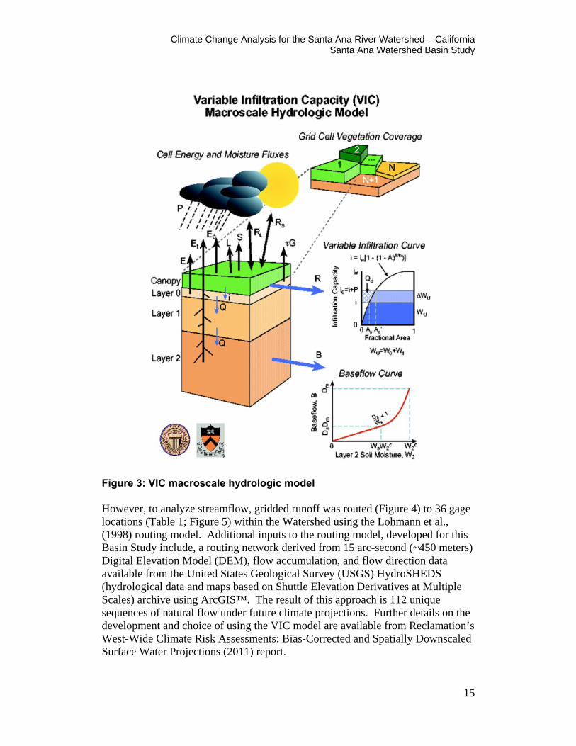
15
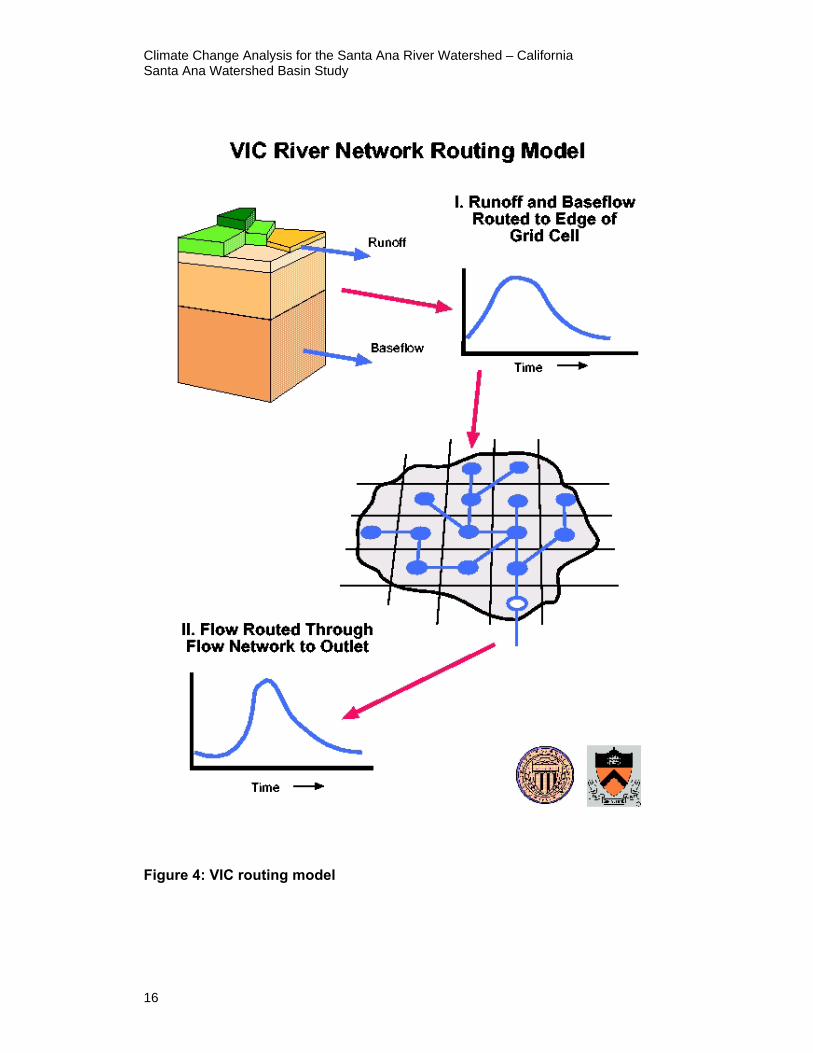
Figure 3: VIC macroscale hydrologic model However, to analyze streamflow, gridded runoff was routed (Figure 4) to 36 gage locations (Table 1; Figure 5) within the Watershed using the Lohmann et al., (1998) routing model. Additional inputs to the routing model, developed for this Basin Study include, a routing network derived from 15 arc-second (~450 meters) Digital Elevation Model (DEM), flow accumulation, and flow direction data available from the United States Geological Survey (USGS) HydroSHEDS (hydrological data and maps based on Shuttle Elevation Derivatives at Multiple Scales) archive using ArcGIS™. The result of this approach is 112 unique sequences of natural flow under future climate projections. Further details on the development and choice of using the VIC model are available from Reclamation’s West-Wide Climate Risk Assessments: Bias-Corrected and Spatially Downscaled Surface Water Projections (2011) report.
Climate Change Analysis for the Santa Ana River Watershed – California Santa Ana Watershed Basin Study
16
Figure 4: VIC routing model

Climate Change Analysis for the Santa Ana River Watershed – California Santa Ana Watershed Basin Study
17
Table 1: Routing locations in the Santa Ana River Watershed
IDLatitude
(decimal degree)Longitude
(decimal degree) Site Description1 33.675020160 -117.835611000 Peters Canyon Wash Tustin Gage
2 33.683909460 -117.745330710 Marshburn Channel Gage
3 33.681686820 -117.809499150 San Diego Creek Myford Rd Gage
4 33.725442191 -117.802408768 El Modina-Irvine Channel Gage
5 33.693809460 -117.823037908 Peters Canyon Wash Irvine Gage
6 33.672798000 -117.835888800 San Diego Creek Lane Rd Gage
7 33.655576290 -117.845611300 San Diego Creek Campus Dr Gage
8 33.885294816 -117.651816486 Santa Ana River Prado Dam Gage
9 33.872738742 -117.670852174 Santa Ana River County Line Gage
10 33.856404490 -117.790611220 Santa Ana River Imperial Highway Gage
11 33.855848910 -117.797555880 Santa Ana River AB SPRD Imperial Highway Gage
12 33.856404440 -117.800889300 Santa Ana River SPRD Imperial Highway Gage
13 33.888903530 -117.845335820 Carbon Creek Olinda Gage
14 33.889459080 -117.845335830 Carbon Creek Yorba Linda Gage
15 33.818812586 -117.873013779 Santa Ana River Ball Rd Gage
16 33.802238450 -117.878390750 Santa Ana River Katella Ave Gage
17 33.822794190 -117.776721310 Santiago Creek Villa Park Gage
18 33.822794190 -117.776721310 Santiago Creek Div Villa Park Gage
19 33.777261477 -117.878057039 Santiago Creek Santa Ana Gage
20 33.752045602 -117.906379262 Santa Ana River Santa Ana Gage
21 33.672033347 -117.943733939 Santa Ana River Adams St Gage
22 33.887792060 -117.926449600 Brea Channel Brea Dam Gage
23 33.873625670 -117.925893710 Brea Channel Fullerton Gage
24 33.895847650 -117.886170600 Fullteron Channel Fullerton Dam Gage
25 33.872875108 -117.902127395 Fullerton Channel Fullerton Gage
26 33.860696271 -117.929366516 Fullerton Channel Richman Ave Gage
27 33.810571570 -118.075342080 Coyote Creek Los Alamitos Gage
28 34.259256110 -117.330684440 Devils Canyon
29 33.968611110 -117.447500000 Santa Ana River AT Metropolitan Water District Crossing NR Arlington
30 34.064688346 -117.303911477 Santa Ana River AT E Street NR San Bernardino
31 33.889166670 -117.561944440 Temescal Creek AB Main Street AT Corona
32 33.982777780 -117.598611110 Cucamonga Creek NR Mira Loma
33 34.003888890 -117.726111110 Chino Creek AT Schaefer Avenue NR Chino
34 34.114206940 -117.096661940 Seven Oaks Dam Outlet
35 34.252500000 -117.525277780 Middle Fork Lytle Creek Gage
36 34.263888890 -117.401388890 Ridge Top Gage NR Devore
Climate Change Analysis for the Santa Ana River Watershed – California Santa Ana Watershed Basin Study
18
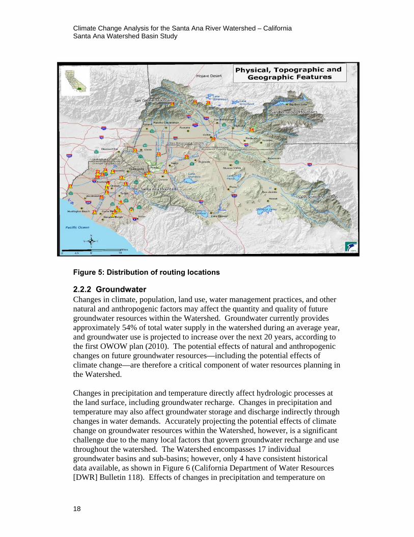
Figure 5: Distribution of routing locations
2.2.2 Groundwater Changes in climate, population, land use, water management practices, and other natural and anthropogenic factors may affect the quantity and quality of future groundwater resources within the Watershed. Groundwater currently provides approximately 54% of total water supply in the watershed during an average year, and groundwater use is projected to increase over the next 20 years, according to the first OWOW plan (2010). The potential effects of natural and anthropogenic changes on future groundwater resources—including the potential effects of climate change—are therefore a critical component of water resources planning in the Watershed. Changes in precipitation and temperature directly affect hydrologic processes at the land surface, including groundwater recharge. Changes in precipitation and temperature may also affect groundwater storage and discharge indirectly through changes in water demands. Accurately projecting the potential effects of climate change on groundwater resources within the Watershed, however, is a significant challenge due to the many local factors that govern groundwater recharge and use throughout the watershed. The Watershed encompasses 17 individual groundwater basins and sub-basins; however, only 4 have consistent historical data available, as shown in Figure 6 (California Department of Water Resources [DWR] Bulletin 118). Effects of changes in precipitation and temperature on

Climate Change Analysis for the Santa Ana River Watershed – California Santa Ana Watershed Basin Study
19
groundwater resources are likely to vary substantially between groundwater basins due to differences in local hydrologic, geologic, and topographic conditions, as well as differences in local water supplies, water demands, and water management practices between basins.
Figure 6: Groundwater basins and monitoring well locations (illustrated by red dots) The effects of climate change on groundwater resources are commonly evaluated using a spatially distributed numerical model of the groundwater flow system in question, which may consist of a single aquifer or unit, multiple aquifers, or an entire groundwater basin or sub-basin. A numerical model of the groundwater flow system is constructed to represent the relevant physical properties of the system, including its geographic extent and orientation, the porosity and permeability of subsurface materials, and the location and extent of key features affecting groundwater flow such as faults, aquitards, and aquicludes. Historical inflows and outflows from the groundwater system are estimated from available data and formatted as model inputs, including spatially distributed recharge from precipitation, focused recharge from stream and canal seepage losses or deep percolation of irrigation water, groundwater abstraction by pumping, and other inflows and outflows. The model is then calibrated and verified with respect to available observations. A second set of groundwater inflows and outflows is then developed based on projected future climate conditions, and is again formatted as model inputs. Finally, the model is used to simulate groundwater flow and storage under historical and projected climate conditions and the resulting model
Upper Santa Ana Valley
Elsinore
San Jacinto
Orange County

Climate Change Analysis for the Santa Ana River Watershed – California Santa Ana Watershed Basin Study
20
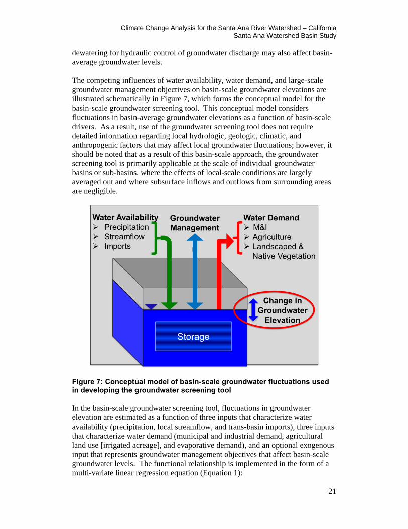
outputs are compared to evaluate the effects of climate change on groundwater resources. The use of spatially-distributed numerical models to evaluate climate change impacts on groundwater is both data intensive and computationally intensive, and requires explicit representation of the many local factors that affect groundwater recharge and use. As a result, this approach generally bears a large cost and long timeline. Moreover, the use of spatially-distributed numerical models to evaluate climate change impacts on groundwater resources in the Watershed would require development of separate models for individual groundwater basins and sub-basins. The cost of such an analysis is therefore prohibitive at the watershed scale. In order to evaluate basin-scale groundwater conditions in the Watershed under future climate, population, land use, and water management scenarios, a basin-scale groundwater screening tool was developed based on a simplified representation of individual groundwater basins. The groundwater screening tool estimates fluctuations in basin-scale groundwater levels in response to natural and anthropogenic drivers, including climate and hydrologic conditions, agricultural land use, municipal water demand, and trans-basin water imports. The tool allows users to quickly estimate basin-scale groundwater conditions under a broad range of future scenarios and provides insight into the primary factors driving basin-scale groundwater fluctuations. A basin-scale groundwater screening tool was developed to facilitate evaluation of groundwater conditions within the Watershed under future climate, population, land use, and water management scenarios. The tool estimates fluctuations in average groundwater levels over a given groundwater basin, at a monthly time scale, in response to natural and anthropogenic drivers, including climate and hydrologic conditions, agricultural land use, municipal water demand, and trans-basin water imports. The tool allows users to quickly estimate changes in basin-average groundwater levels in response to projected changes in future climate, and provides insight into the primary factors driving basin-scale groundwater fluctuations. In groundwater basins where groundwater is a primary source of water supply, fluctuations in basin-averaged groundwater level depend on both water availability and water demands. In general, higher than average water availability from precipitation, local streamflow, and imported water contributes to increased recharge and/or decreased groundwater pumping, resulting in rising groundwater levels. By contrast, higher than average water demands for municipal and agricultural uses and higher than average evaporative demand from native and landscaped vegetation contribute to decreased recharge and/or increased groundwater pumping, resulting in declining groundwater levels. In addition to supply and demand, large-scale management objectives in some groundwater basins such as pressurization of hydraulic barriers against sea water intrusion and
Climate Change Analysis for the Santa Ana River Watershed – California Santa Ana Watershed Basin Study
21
dewatering for hydraulic control of groundwater discharge may also affect basin-average groundwater levels. The competing influences of water availability, water demand, and large-scale groundwater management objectives on basin-scale groundwater elevations are illustrated schematically in Figure 7, which forms the conceptual model for the basin-scale groundwater screening tool. This conceptual model considers fluctuations in basin-average groundwater elevations as a function of basin-scale drivers. As a result, use of the groundwater screening tool does not require detailed information regarding local hydrologic, geologic, climatic, and anthropogenic factors that may affect local groundwater fluctuations; however, it should be noted that as a result of this basin-scale approach, the groundwater screening tool is primarily applicable at the scale of individual groundwater basins or sub-basins, where the effects of local-scale conditions are largely averaged out and where subsurface inflows and outflows from surrounding areas are negligible.
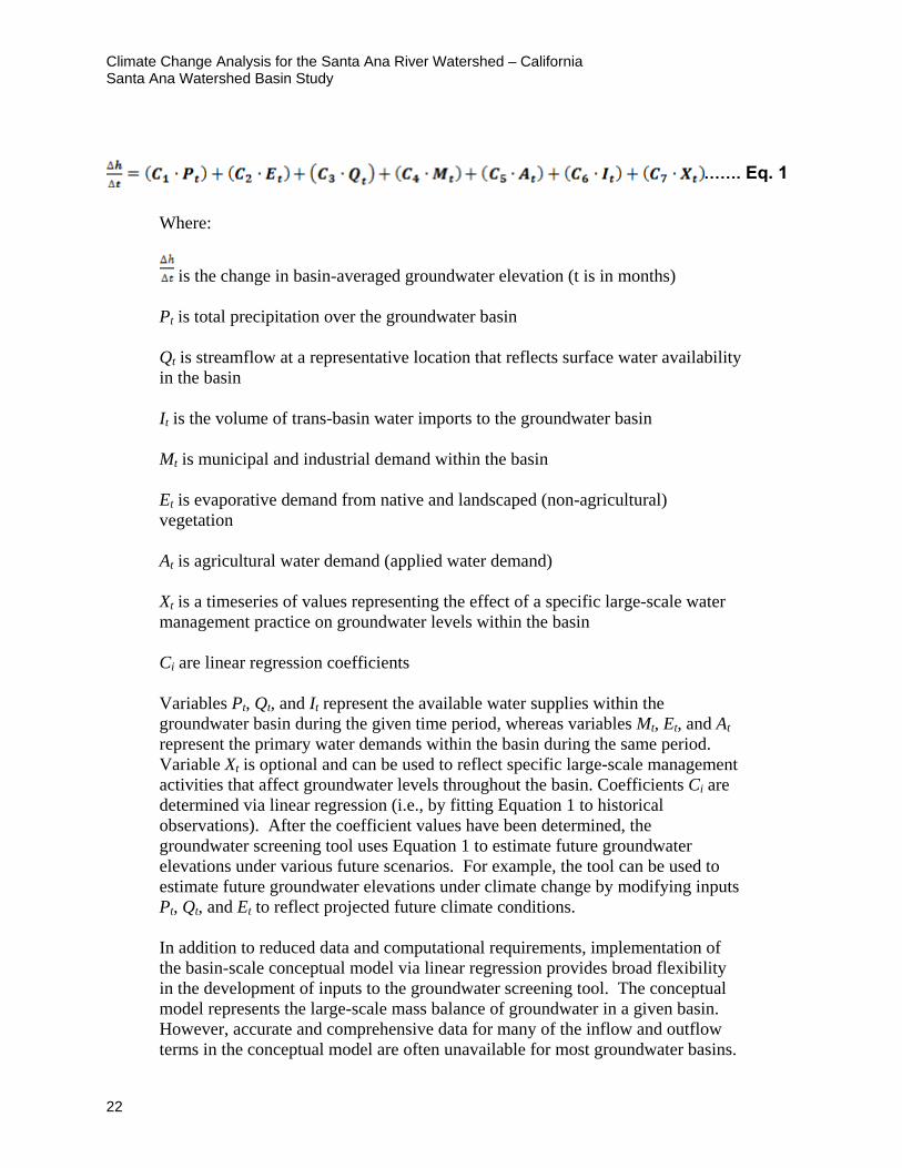
Figure 7: Conceptual model of basin-scale groundwater fluctuations used in developing the groundwater screening tool In the basin-scale groundwater screening tool, fluctuations in groundwater elevation are estimated as a function of three inputs that characterize water availability (precipitation, local streamflow, and trans-basin imports), three inputs that characterize water demand (municipal and industrial demand, agricultural land use [irrigated acreage], and evaporative demand), and an optional exogenous input that represents groundwater management objectives that affect basin-scale groundwater levels. The functional relationship is implemented in the form of a multi-variate linear regression equation (Equation 1):
Climate Change Analysis for the Santa Ana River Watershed – California Santa Ana Watershed Basin Study
22
……. Eq. 1 Where:
is the change in basin-averaged groundwater elevation (t is in months) Pt is total precipitation over the groundwater basin Qt is streamflow at a representative location that reflects surface water availability in the basin It is the volume of trans-basin water imports to the groundwater basin Mt is municipal and industrial demand within the basin Et is evaporative demand from native and landscaped (non-agricultural) vegetation At is agricultural water demand (applied water demand) Xt is a timeseries of values representing the effect of a specific large-scale water management practice on groundwater levels within the basin Ci are linear regression coefficients Variables Pt, Qt, and It represent the available water supplies within the groundwater basin during the given time period, whereas variables Mt, Et, and At represent the primary water demands within the basin during the same period. Variable Xt is optional and can be used to reflect specific large-scale management activities that affect groundwater levels throughout the basin. Coefficients Ci are determined via linear regression (i.e., by fitting Equation 1 to historical observations). After the coefficient values have been determined, the groundwater screening tool uses Equation 1 to estimate future groundwater elevations under various future scenarios. For example, the tool can be used to estimate future groundwater elevations under climate change by modifying inputs Pt, Qt, and Et to reflect projected future climate conditions. In addition to reduced data and computational requirements, implementation of the basin-scale conceptual model via linear regression provides broad flexibility in the development of inputs to the groundwater screening tool. The conceptual model represents the large-scale mass balance of groundwater in a given basin. However, accurate and comprehensive data for many of the inflow and outflow terms in the conceptual model are often unavailable for most groundwater basins.

Climate Change Analysis for the Santa Ana River Watershed – California Santa Ana Watershed Basin Study
23
For example, evaporative demand for native and landscaped vegetation generally is not readily available for most groundwater basins. The regression-based approach used here allows the user to substitute a related variable in place of the missing data. In the case of evaporative demand, the user may substitute temperature data for evaporative demand as temperature is strongly correlated with evaporative demand. As long as fluctuations in the substituted dataset (in this case temperature) are strongly correlated with fluctuations in the primary input variable (in this case evaporative demand), discrepancies in magnitudes of two variables are accounted for by the regression coefficient on this term.
Development of Groundwater Model Inputs As detailed above, the groundwater screening tool estimates changes in basin-averaged groundwater levels over time as a function of seven natural and anthropogenic factors that govern groundwater recharge and discharge: precipitation, local streamflow, trans-basin water imports, municipal and industrial water demands, agricultural water demand, evaporative demand from native and landscaped vegetation (non-agricultural), and an optional exogenous input that represents groundwater management objectives that affect basin-scale groundwater levels. The regression-based approach used in the groundwater screening tool allows substitution of related datasets where accurate data for one or more model input is not available. This section summarizes the development of inputs to the groundwater screening tool for groundwater basins within the Watershed.
Historical Input Data (1990-2009) Historical data were used to fit the regression coefficients in Equation 1 and to evaluate model performance over the historical period (1990-2009). For each groundwater basin, historical inputs are required for the six primary input variables to Equation 1. Additional inputs may be provided for the optional exogenous variable if desired. No exogenous inputs were developed for groundwater basins within the Watershed; however, exogenous inputs may be incorporated by water resources planners and decision makers in the watershed based on knowledge of management operations relevant to individual groundwater basins.
Groundwater Elevation (ht) The groundwater screening tool requires an input timeseries representative of historical monthly groundwater elevations within the basin for the period 1990-2009. For this study, a database of historical groundwater elevations from more than 4,000 monitoring wells within the Watershed was obtained from SAWPA. Monitoring well locations are shown in Figure 6. Well records were evaluated to determine the period of record, completeness of record, and occurrence of outlier or spurious values. Wells exhibiting records shorter than 10 consecutive years or exhibiting a high frequency of missing values were excluded from this analysis. For each well identified as having a sufficient period of record and sufficient sampling frequency, monthly mean groundwater elevations were calculated from the available instantaneous measurements. For months containing more than one
Climate Change Analysis for the Santa Ana River Watershed – California Santa Ana Watershed Basin Study
24
measurement, the monthly average was computed as the unweighted arithmetic average of the available measurements. For months with a single measurement, the single measurement was assumed to reflect average conditions during that month. It should be noted that individual outlier points were excluded from averaging; outliers likely reflect measurement errors, data transcription errors, or measurements taken during or after permeability testing was carried out (i.e., during or after a slug test or pump test). Lastly, monthly averages were linearly interpolated to develop a complete timeseries of monthly mean groundwater elevations over the period of record. Accuracy of monthly timeseries was evaluated by sub-sampling and cross-validation. Interpolated monthly timeseries were shown to accurately reflect raw measurements. Monthly timeseries of basin-averaged groundwater elevations were then developed for each of the individual groundwater basins and sub-basins (defined by DWR) in the Watershed. Steps were required to avoid two sources of bias in calculating basin-average groundwater elevations: variations in the period of record between wells, and outlier wells that are not representative of large-scale groundwater fluctuations within a basin. These steps are described below. Very few wells in the database used here exhibit complete monthly timeseries for the full historical period (1990-2009). As a result, simply taking the arithmetic average of well records over each groundwater basin results in a biased estimate of basin-average groundwater elevations. This bias occurs due to differences in the period of record of wells within a given basin: if the basin average for different months is based on a different sub-set of wells, and each well has a different mean groundwater elevation, then the resulting average reflects variations in the sub-set of well used. To minimize biases associated with varying record lengths, averaging was carried out based on monthly deviations rather than monthly groundwater elevations. This was done by computing monthly deviations (anomalies) for each record (i.e. for each well), where monthly deviations are calculated as the difference between the monthly mean value and the long-term average value for that month. In addition to differences in record length, potential biases may occur in cases where individual well records reflect unique local conditions that are not broadly representative of groundwater fluctuations within the basin. This situation might occur when groundwater pumping throughout a basin is not driven primarily by municipal and industrial demand, but is driven by agricultural demand in one small area of the basin. Groundwater fluctuations in the agricultural portion of the basin are likely to exhibit substantially different behavior than groundwater fluctuations throughout the rest of the basin. In basins where a large number of monitoring wells are available, individual outliers have little effect on the basin-scale average and therefore do not need to be excluded from analysis. Where a small number of samples are available, however, individual outliers can disproportionately impact the basin average, resulting in potentially significant bias.
Climate Change Analysis for the Santa Ana River Watershed – California Santa Ana Watershed Basin Study
25
For this study, a correlation-based clustering procedure was developed to group wells into sub-sets exhibiting similar behavior. In basins and sub-basins where a large number of monitoring records were available, the majority of wells fell into a single cluster. For the purposes of this analysis, the largest cluster was assumed to reflect basin-average conditions, and basin-average groundwater elevations were calculated based on wells in this cluster. In basins and sub-basins where, only a small number of records were available, wells generally fell into a small number of similar size clusters. For the purposes of this analysis, these clusters were assumed to represent conditions in different portions of the basin where groundwater fluctuations were subject to different primary stressors. In these cases, averages were computed for each cluster and were evaluated separately. This report only presents results for basins where the majority of groundwater records fell into a single cluster.
Precipitation (Pt) The groundwater screening tool requires an input timeseries that is representative of historical monthly precipitation over the groundwater basin for the period 1990-2009. Precipitation input may be basin-averaged monthly precipitation calculated from multiple gage records or from a gridded precipitation dataset. Alternatively, precipitation input may be derived from gage data at a single location or selected locations that represent key areas within the groundwater basin, such as areas of significant recharge or runoff. For this study, basin-average monthly precipitation was calculated for each groundwater basin based on the historical gridded daily precipitation dataset developed by Maurer et al. (2002), the same dataset used to derive the surface water projections. Area-weighted monthly total precipitation was computed for each basin based on groundwater basin polygons developed by DWR.
Evaporative Demand (Et) The groundwater screening tool requires an input timeseries that is representative of historical monthly evaporative demand from native and landscaped (non-agricultural) vegetation over the groundwater basin for the period 1990-2009. Because evaporative demand is generally not measured directly, monthly mean temperature or calculated monthly potential evapotranspiration (PET) may be used as surrogates for evaporative demand. For this study, basin-average monthly-mean temperature was calculated for each groundwater basin based on the historical gridded daily temperature dataset developed by Maurer et al. (2002), the same dataset used to derive the surface water hydrology projections. Area-weighted monthly-mean temperature was computed for each basin based on groundwater basin polygons developed by DWR.
Streamflow (Qt) The groundwater screening tool requires an input timeseries that is representative of historical monthly streamflow that contributed to water supply in the groundwater basin for the period 1990-2009. This streamflow excludes that
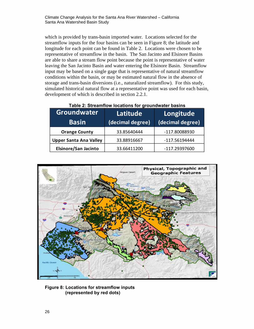
Climate Change Analysis for the Santa Ana River Watershed – California Santa Ana Watershed Basin Study
26
which is provided by trans-basin imported water. Locations selected for the streamflow inputs for the four basins can be seen in Figure 8; the latitude and longitude for each point can be found in Table 2. Locations were chosen to be representative of streamflow in the basin. The San Jacinto and Elsinore Basins are able to share a stream flow point because the point is representative of water leaving the San Jacinto Basin and water entering the Elsinore Basin. Streamflow input may be based on a single gage that is representative of natural streamflow conditions within the basin, or may be estimated natural flow in the absence of storage and trans-basin diversions (i.e., naturalized streamflow). For this study, simulated historical natural flow at a representative point was used for each basin, development of which is described in section 2.2.1.
Table 2: Streamflow locations for groundwater basins
Figure 8: Locations for streamflow inputs (represented by red dots)
Groundwater Basin
Latitude (decimal degree)
Longitude (decimal degree)
Orange County 33.85640444 -117.80088930
Upper Santa Ana Valley 33.88916667 -117.56194444
Elsinore/San Jacinto 33.66411200 -117.29397600
Climate Change Analysis for the Santa Ana River Watershed – California Santa Ana Watershed Basin Study
27
Municipal and Industrial Demand (Mt) The groundwater screening tool requires an input timeseries that is representative of historical monthly municipal and industrial water demand within the groundwater basin for the period 1990-2009. Where municipal and industrial demand data are not directly available, demand may be estimated from available population and per capita water use data, interpolated as needed to obtain monthly data for the period 1990-2009. For this study, population within each groundwater basin was calculated from census tract data for years 1990, 2000, and 2010, and were interpolated to obtain monthly values. Data for annual per capita water use were obtained from urban water management plans for SAWPA member agencies and other water providers within each basin, and were similarly interpolated to obtain monthly values. Municipal and industrial demand was then estimated as the product of population and per capita use.
Agricultural Demand (At) The groundwater screening tool requires an input timeseries that is representative of historical monthly agricultural water demand within the groundwater basin for the period 1990-2009. Accurate and consistent data on agricultural water use is not available for the groundwater basins within the Watershed. For this study, agricultural land area (irrigated acreage) was used as a surrogate for agricultural demand. For each groundwater basin, irrigated acreage was calculated from available land use datasets developed by the Southern California Association of Governments (SCAG). Available values were interpolated to obtain estimates of monthly values over the period 1990-2009. Where cropping patterns and irrigation practices are reasonably constant, agricultural acreage is strongly correlated with agricultural demand.
Trans-basin Imported Water (It) The groundwater screening tool requires an input timeseries that is representative of historical monthly trans-basin water imported into the groundwater basin for the period 1990-2009. For this study, import data were obtained from SAWPA member agencies and associated, to the extent possible, with the corresponding groundwater basin. Initial analysis revealed that trans-basin imports are generally small compared to precipitation and natural streamflow for most groundwater basins in the watershed; as a result, uncertainties associated with the historical trans-basin import data used in this analysis is considered negligible.
Exogenous Variable (Xt) The simplified approach used by the groundwater screening tool does not represent many of the complex and dynamic processes that may affect groundwater fluctuations within a given basin. For this purpose, the tool allows for an optional exogenous input, which provides the user an opportunity to account for a key driver that is not explicitly represented by the above inputs. Key drivers may include groundwater injection operations for a hydraulic barrier against sea water intrusion, dewatering for hydraulic control of groundwater

Climate Change Analysis for the Santa Ana River Watershed – California Santa Ana Watershed Basin Study
28
discharge, or other management objectives that affect groundwater levels. No exogenous variable was used in this study.
Projected (Future) Input Data (2010-2099) The groundwater screening tool estimates future groundwater elevations over the period 2010-2099 based on input data reflecting projected water supply, water demand, and water management conditions over this period. Future inputs are required for each of the primary input variables to the screening tool. If an exogenous variable is used for the historical period, projected values of the same exogenous variable are required for the future period. As noted above, no exogenous inputs were developed for groundwater basins within the Watershed. It should also be noted that projected groundwater elevations are calculated by the screening tool; groundwater elevation is not an input for the future period.
Precipitation (Pt) The groundwater screening tool allows users to provide up to 250 projections of future precipitation for a given basin. Consideration of multiple future projections provides insight into the range of future conditions corresponding to uncertainties in projected future climate. For this study, projected basin-average monthly precipitation for the period 2010-2099 was calculated based on an ensemble of 112 bias corrected and spatially disaggregated climate projections (see Section 2.2.1). For each projection, input timeseries were developed by calculating the area-weighted monthly total precipitation for groundwater basin polygons developed by DWR.
Evaporative Demand (Et) Similar to precipitation, the groundwater screening tool allows users to provide up to 250 projections of future evaporative demand for a given basin. For consistency with historical inputs, basin-average monthly-mean temperature was used to represent monthly evaporative demand over the future period. Projected basin-average monthly average temperature inputs were calculated for each groundwater basin based on an ensemble of 112 BCSD climate projections (see Section 2.2.1). For each projection, input timeseries were developed by calculating the area-weighted monthly average temperature for groundwater basin polygons developed by DWR.
Streamflow (Qt) Similar to precipitation and temperature, the groundwater screening tool allows users to provide up to 250 projections of streamflow for a given basin. For this study, projected natural flow at a representative point for the period 2010-2099 was used for each basin (see Section 2.2.1).
Municipal and Industrial Demand (Mt) The groundwater screening tool requires a single timeseries input representing projected municipal and industrial demand for the future period. For the purposes of this study, it was assumed that future municipal and industrial demand will
Climate Change Analysis for the Santa Ana River Watershed – California Santa Ana Watershed Basin Study
29
remain at current levels. However, the tool allows water resources planners and decision makers to input alternative projections of future municipal and industrial demand based on various scenarios and planning objectives related to individual groundwater basins.
Agricultural Demand (At) The groundwater screening tool requires a single timeseries input representing projected agricultural demand for the future period. For consistency with historical inputs, agricultural land area (irrigated acreage) was used to represent agricultural water demand in the future. For the purposes of this study, it was assumed that future agricultural land area will remain at current levels. However, the tool allows water resources planners and decision makers to input alternative projections of future agricultural demand based on various scenarios and planning objectives related to individual groundwater basins.
Trans-basin Imported Water (It) The groundwater screening tool requires a single timeseries input representing projected trans-basin imported water for the future period. For the purposes of this study, it was assumed that future water imports will remain at the average historical level, calculated as the average over the period 1990-2009. However, the tool allows water resources planners and decision makers to input alternative projections of future water imports based on various scenarios and planning objectives related to individual groundwater basins.
Exogenous Variable (Xt) As for the historical period, no exogenous variable was used in this study for the future period. The methods described in this chapter were used to project hydroclimate conditions including surface water and groundwater supplies, which are presented in Chapter 3 along with projected demand.

Climate Change Analysis for the Santa Ana River Watershed – California Santa Ana Watershed Basin Study
30
3.0 Water Supply and Demand Projections
3.1 Water Supply
Future water supply projections were made using the CMIP3 projections and the VIC hydrology model. The CMIP3 archive provides a downscaled 12 kilometer resolution grid on a monthly time-series of precipitation and temperature from 1950-2099 for 112 climate projections.
3.1.1 Hydroclimate Projections
Timeseries Plots This set includes projection specific annual timeseries plots for six hydroclimate indicator variables covering the period 1950–2099 (water years 1951-2099). The six variables are:
• Annual Total Precipitation • Annual Mean Temperature • April 1st Snow Water Equivalent • Annual Runoff • December–March Runoff • April–July Runoff
The three variables—annual total precipitation, annual mean temperature, and April 1st SWE—vary spatially (at 1/8° or ~ 12-km-grid resolution) across the basins. To estimate total annual precipitation for the basin, basin-wide average precipitation (average across the grid cells in the basin) was first calculated for each month of the years 1950–2099. These basin average monthly precipitation values then were summed for each water year 1951-2099 to obtain the annual total precipitation. To estimate basin mean temperature, average monthly temperature was calculated from all the grid cells in the basin for each month of the water years 1951–2099. These monthly temperatures for any given year next were averaged across the grid cells in the basin to estimate the basin-wide annual mean temperature. SWE on April 1st of a given year is a widely used measure to assess snowpack and subsequent spring–summer runoff conditions in the snowmelt dominated basins of the western United States. SWE is one possible output from the VIC hydrology model. For each of the simulation water years, April 1st SWE was
Climate Change Analysis for the Santa Ana River Watershed – California Santa Ana Watershed Basin Study
31
saved from the simulations for each model grid cell in the basin. Gridded SWE on April 1st was averaged over all the grid cells for the given basin to calculate the basin-wide April 1st SWE for water years, 1950–2099. Runoff for each of the 36 site locations (Table 1) was calculated for the annual timescale and for two seasonal timescales December–March (DJFM) total runoff depicting winter season runoff conditions and April–July (AMJJ) total runoff depicting spring–summer runoff conditions. For each of the simulation years 1950–2099, monthly runoff was aggregated on a water year basis to calculate water year specific total annual runoff, DJFM runoff, and AMJJ runoff. The annual time series plots for the six hydrologic indicator variables for all 112 projections were calculated, and the results are presented to reflect ensemble central tendency and ensemble spread. The central tendency is measured using the ensemble median. The 5th and 95th percentiles from the 112 projections provide the lower and upper uncertainty bounds in the envelope of projections through time. Figure 9 shows the projection ensemble for six hydroclimate indicators for the site Santa Ana River at Adams Street Gage (most downstream location): annual total precipitation (top left), annual mean temperature (top right), April 1st SWE (middle left), annual runoff (middle right), DJFM runoff season (bottom left), and AMJJ runoff season (bottom right). The heavy black line is the annual time series of 50th percentile values (i.e., ensemble-median). The shaded area is the annual time series of 5th to 95th percentiles. The annual total precipitation over the basin shows a somewhat declining trend over the transient period going out to 2099. The uncertainty envelope does not appear to expand or contract over time. The mean annual temperature over the basin shows a monotonically increasing trend and a diverging uncertainty envelope over time. April 1st SWE also shows a decreasing trend. The annual runoff follows the long-term declining trend pattern similar to precipitation. The winter season DJFM runoff shows a declining trend, so does the AMJJ summer season runoff.
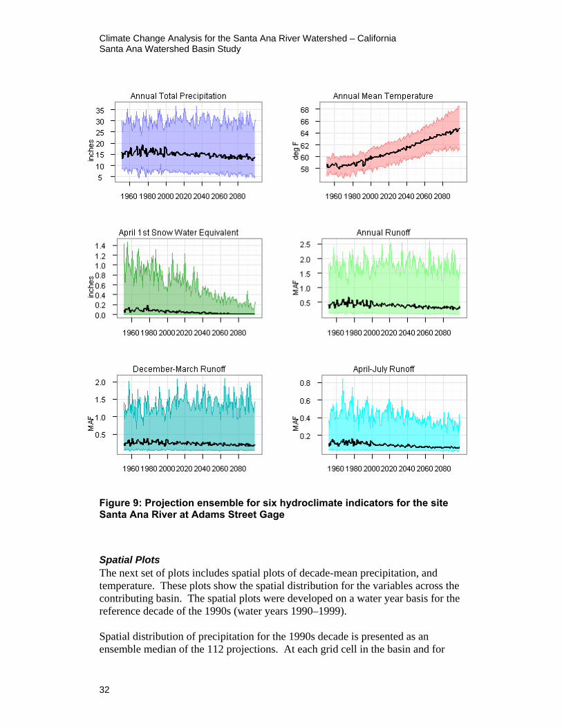
Climate Change Analysis for the Santa Ana River Watershed – California Santa Ana Watershed Basin Study
32
Figure 9: Projection ensemble for six hydroclimate indicators for the site Santa Ana River at Adams Street Gage
Spatial Plots The next set of plots includes spatial plots of decade-mean precipitation, and temperature. These plots show the spatial distribution for the variables across the contributing basin. The spatial plots were developed on a water year basis for the reference decade of the 1990s (water years 1990–1999). Spatial distribution of precipitation for the 1990s decade is presented as an ensemble median of the 112 projections. At each grid cell in the basin and for
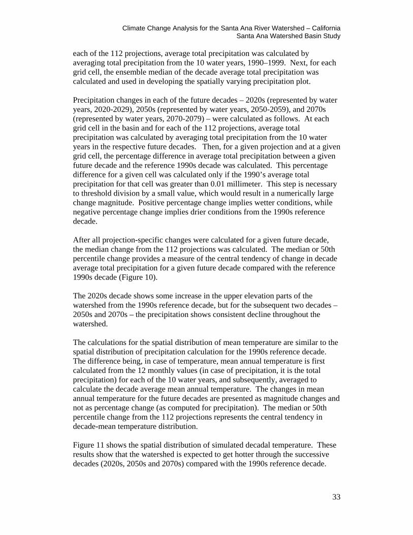
Climate Change Analysis for the Santa Ana River Watershed – California Santa Ana Watershed Basin Study
33
each of the 112 projections, average total precipitation was calculated by averaging total precipitation from the 10 water years, 1990–1999. Next, for each grid cell, the ensemble median of the decade average total precipitation was calculated and used in developing the spatially varying precipitation plot. Precipitation changes in each of the future decades – 2020s (represented by water years, 2020-2029), 2050s (represented by water years, 2050-2059), and 2070s (represented by water years, 2070-2079) – were calculated as follows. At each grid cell in the basin and for each of the 112 projections, average total precipitation was calculated by averaging total precipitation from the 10 water years in the respective future decades. Then, for a given projection and at a given grid cell, the percentage difference in average total precipitation between a given future decade and the reference 1990s decade was calculated. This percentage difference for a given cell was calculated only if the 1990’s average total precipitation for that cell was greater than 0.01 millimeter. This step is necessary to threshold division by a small value, which would result in a numerically large change magnitude. Positive percentage change implies wetter conditions, while negative percentage change implies drier conditions from the 1990s reference decade. After all projection-specific changes were calculated for a given future decade, the median change from the 112 projections was calculated. The median or 50th percentile change provides a measure of the central tendency of change in decade average total precipitation for a given future decade compared with the reference 1990s decade (Figure 10). The 2020s decade shows some increase in the upper elevation parts of the watershed from the 1990s reference decade, but for the subsequent two decades – 2050s and 2070s – the precipitation shows consistent decline throughout the watershed. The calculations for the spatial distribution of mean temperature are similar to the spatial distribution of precipitation calculation for the 1990s reference decade. The difference being, in case of temperature, mean annual temperature is first calculated from the 12 monthly values (in case of precipitation, it is the total precipitation) for each of the 10 water years, and subsequently, averaged to calculate the decade average mean annual temperature. The changes in mean annual temperature for the future decades are presented as magnitude changes and not as percentage change (as computed for precipitation). The median or 50th percentile change from the 112 projections represents the central tendency in decade-mean temperature distribution. Figure 11 shows the spatial distribution of simulated decadal temperature. These results show that the watershed is expected to get hotter through the successive decades (2020s, 2050s and 2070s) compared with the 1990s reference decade.
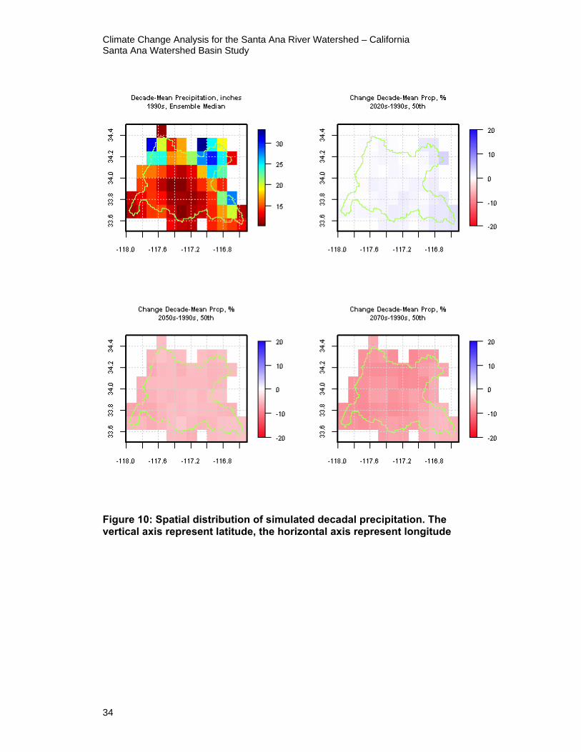
Climate Change Analysis for the Santa Ana River Watershed – California Santa Ana Watershed Basin Study
34
Figure 10: Spatial distribution of simulated decadal precipitation. The vertical axis represent latitude, the horizontal axis represent longitude
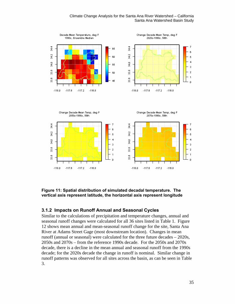
Climate Change Analysis for the Santa Ana River Watershed – California Santa Ana Watershed Basin Study
35
Figure 11: Spatial distribution of simulated decadal temperature. The vertical axis represent latitude, the horizontal axis represent longitude
3.1.2 Impacts on Runoff Annual and Seasonal Cycles Similar to the calculations of precipitation and temperature changes, annual and seasonal runoff changes were calculated for all 36 sites listed in Table 1. Figure 12 shows mean annual and mean-seasonal runoff change for the site, Santa Ana River at Adams Street Gage (most downstream location). Changes in mean runoff (annual or seasonal) were calculated for the three future decades – 2020s, 2050s and 2070s – from the reference 1990s decade. For the 2050s and 2070s decade, there is a decline in the mean annual and seasonal runoff from the 1990s decade; for the 2020s decade the change in runoff is nominal. Similar change in runoff patterns was observed for all sites across the basin, as can be seen in Table 3.

Climate Change Analysis for the Santa Ana River Watershed – California Santa Ana Watershed Basin Study
36
Figure 12: Simulated mean annual and mean-seasonal runoff change
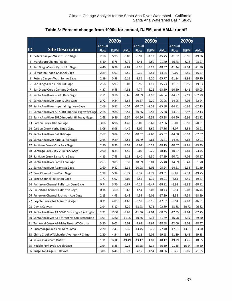
Climate Change Analysis for the Santa Ana River Watershed – California Santa Ana Watershed Basin Study
37
Table 3: Percent change from 1990s for annual, DJFM, and AMJJ runoff
Annual Flow DJFM AMJJ
Annual Flow DJFM AMJJ
Annual Flow DJFM AMJJ
1 Peters Canyon Wash Tustin Gage 2.58 5.95 -6.08 -8.92 -1.19 -15.75 -11.82 -8.96 -19.06
2 Marshburn Channel Gage 5.10 6.76 -8.79 -6.41 -2.60 -21.70 -10.73 -8.12 -23.97
3 San Diego Creek Myford Rd Gage 4.40 6.98 -7.87 -8.36 -3.28 -18.67 -11.44 -7.34 -21.36
4 El Modina-Irvine Channel Gage 2.89 4.01 -3.50 -6.36 -3.54 -14.84 -9.05 -8.46 -15.37
5 Peters Canyon Wash Irvine Gage 2.59 5.98 -6.15 -8.86 -1.20 -15.77 -11.84 -8.98 -19.10
6 San Diego Creek Lane Rd Gage 2.58 5.93 -6.03 -8.95 -1.19 -15.73 -11.81 -8.95 -19.03
7 San Diego Creek Campus Dr Gage 4.37 6.48 -4.81 -7.74 -3.22 -13.80 -10.30 -8.42 -15.05
8 Santa Ana River Prado Dam Gage 2.71 9.76 -6.65 -10.69 -1.90 -26.04 -14.97 -7.19 -32.29
9 Santa Ana River County Line Gage 2.72 9.84 -6.66 -10.67 -2.20 -25.96 -14.95 -7.08 -32.24
10 Santa Ana River Imperial Highway Gage 2.69 9.87 -6.54 -10.57 -2.52 -25.88 -14.91 -6.92 -32.13
11 Santa Ana River AB SPRD Imperial Highway Gage 2.68 9.86 -6.54 -10.56 -2.53 -25.88 -14.91 -6.92 -32.13
12 Santa Ana River SPRD Imperial Highway Gage 2.68 9.86 -6.54 -10.56 -2.53 -25.88 -14.90 -6.92 -32.12
13 Carbon Creek Olinda Gage 3.06 6.96 -4.49 -3.09 -3.69 -17.86 -8.07 -6.58 -20.91
14 Carbon Creek Yorba Linda Gage 3.06 6.96 -4.49 -3.09 -3.69 -17.86 -8.07 -6.58 -20.91
15 Santa Ana River Ball Rd Gage 2.67 9.84 -6.53 -10.52 -2.60 -25.82 -14.88 -6.92 -32.07
16 Santa Ana River Katella Ave Gage 2.65 9.89 -6.55 -10.49 -2.83 -25.71 -14.85 -6.88 -32.01
17 Santiago Creek Villa Park Gage 2.90 8.35 -4.59 -5.09 -0.25 -18.15 -10.07 -7.81 -23.45
18 Santiago Creek Div Villa Park Gage 2.90 8.35 -4.59 -5.09 -0.25 -18.15 -10.07 -7.81 -23.45
19 Santiago Creek Santa Ana Gage 4.15 7.43 -5.11 -5.40 -1.30 -17.99 -10.42 -7.02 -20.97
20 Santa Ana River Santa Ana Gage 2.63 9.85 -6.39 -10.09 -3.01 -25.48 -14.69 -6.41 -31.70
21 Santa Ana River Adams St Gage 2.60 9.82 -6.35 -10.08 -3.01 -25.24 -14.61 -6.38 -31.39
22 Brea Channel Brea Dam Gage 1.99 5.34 -5.77 -3.37 -1.79 -19.51 -8.88 -7.33 -19.75
23 Brea Channel Fullerton Gage 1.73 4.97 -6.04 -3.54 -1.35 -19.91 -8.84 -7.45 -19.87
24 Fullteron Channel Fullerton Dam Gage 0.94 3.76 -5.87 -4.13 -1.47 -18.91 -8.98 -8.82 -18.91
25 Fullerton Channel Fullerton Gage 0.14 3.60 -5.68 -4.54 -3.08 -18.43 -9.14 -9.08 -16.44
26 Fullerton Channel Richman Ave Gage 2.15 4.95 -5.48 -4.55 -2.02 -17.80 -8.58 -7.34 -18.39
27 Coyote Creek Los Alamitos Gage 0.31 4.85 -4.60 -3.59 -3.16 -17.37 -9.54 -7.87 -16.51
28 Devils Canyon 2.94 5.12 -3.29 -13.23 -6.71 -22.69 -13.38 -10.72 -26.62
29 Santa Ana River AT MWD Crossing NR Arlington 2.73 10.54 -9.68 -11.36 -2.04 -30.55 -17.35 -7.84 -37.75
30 Santa Ana River AT E Street NR San Bernardino 3.03 10.66 -11.25 -10.86 -2.34 -31.89 -16.98 -7.35 -39.70
31 Temescal Creek AB Main Street AT Corona 5.50 9.02 -6.01 -7.65 -1.64 -18.68 -12.06 -5.03 -28.47
32 Cucamonga Creek NR Mira Loma 2.20 7.43 -3.35 -13.45 -8.76 -27.40 -17.51 -13.81 -33.20
33 Chino Creek AT Schaefer Avenue NR Chino 2.30 4.54 -3.62 -7.11 -2.05 -19.63 -11.19 -8.46 -19.83
34 Seven Oaks Dam Outlet 1.11 12.83 -19.49 -13.17 -4.07 -40.17 -19.29 -4.76 -48.65
35 Middle Fork Lytle Creek Gage 2.94 6.88 -9.22 -15.28 -8.14 -36.30 -21.35 -16.24 -40.80
36 Ridge Top Gage NR Devore 3.08 6.48 -6.72 -7.15 -1.54 -18.56 -6.26 -5.05 -21.65
2020s 2050s 2070s
ID Site Description
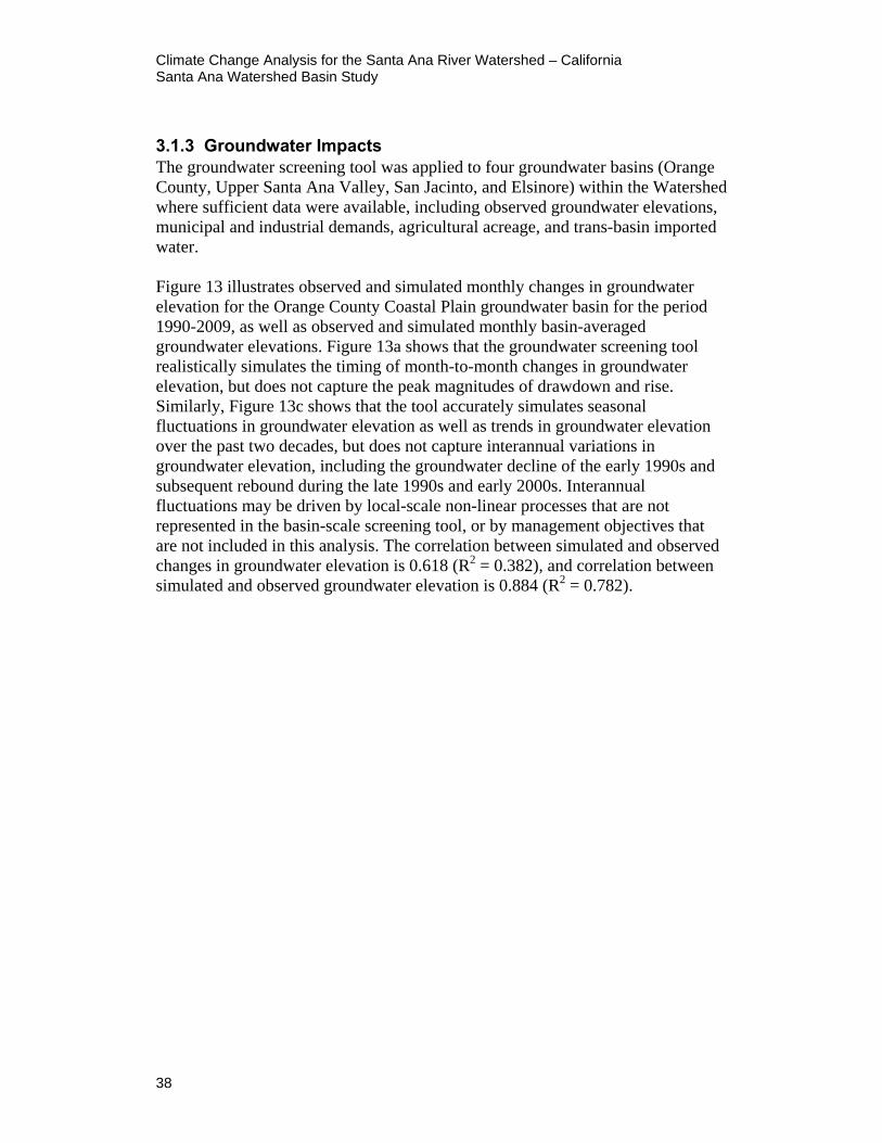
Climate Change Analysis for the Santa Ana River Watershed – California Santa Ana Watershed Basin Study
38
3.1.3 Groundwater Impacts The groundwater screening tool was applied to four groundwater basins (Orange County, Upper Santa Ana Valley, San Jacinto, and Elsinore) within the Watershed where sufficient data were available, including observed groundwater elevations, municipal and industrial demands, agricultural acreage, and trans-basin imported water. Figure 13 illustrates observed and simulated monthly changes in groundwater elevation for the Orange County Coastal Plain groundwater basin for the period 1990-2009, as well as observed and simulated monthly basin-averaged groundwater elevations. Figure 13a shows that the groundwater screening tool realistically simulates the timing of month-to-month changes in groundwater elevation, but does not capture the peak magnitudes of drawdown and rise. Similarly, Figure 13c shows that the tool accurately simulates seasonal fluctuations in groundwater elevation as well as trends in groundwater elevation over the past two decades, but does not capture interannual variations in groundwater elevation, including the groundwater decline of the early 1990s and subsequent rebound during the late 1990s and early 2000s. Interannual fluctuations may be driven by local-scale non-linear processes that are not represented in the basin-scale screening tool, or by management objectives that are not included in this analysis. The correlation between simulated and observed changes in groundwater elevation is 0.618 (R2 = 0.382), and correlation between simulated and observed groundwater elevation is 0.884 (R2 = 0.782).
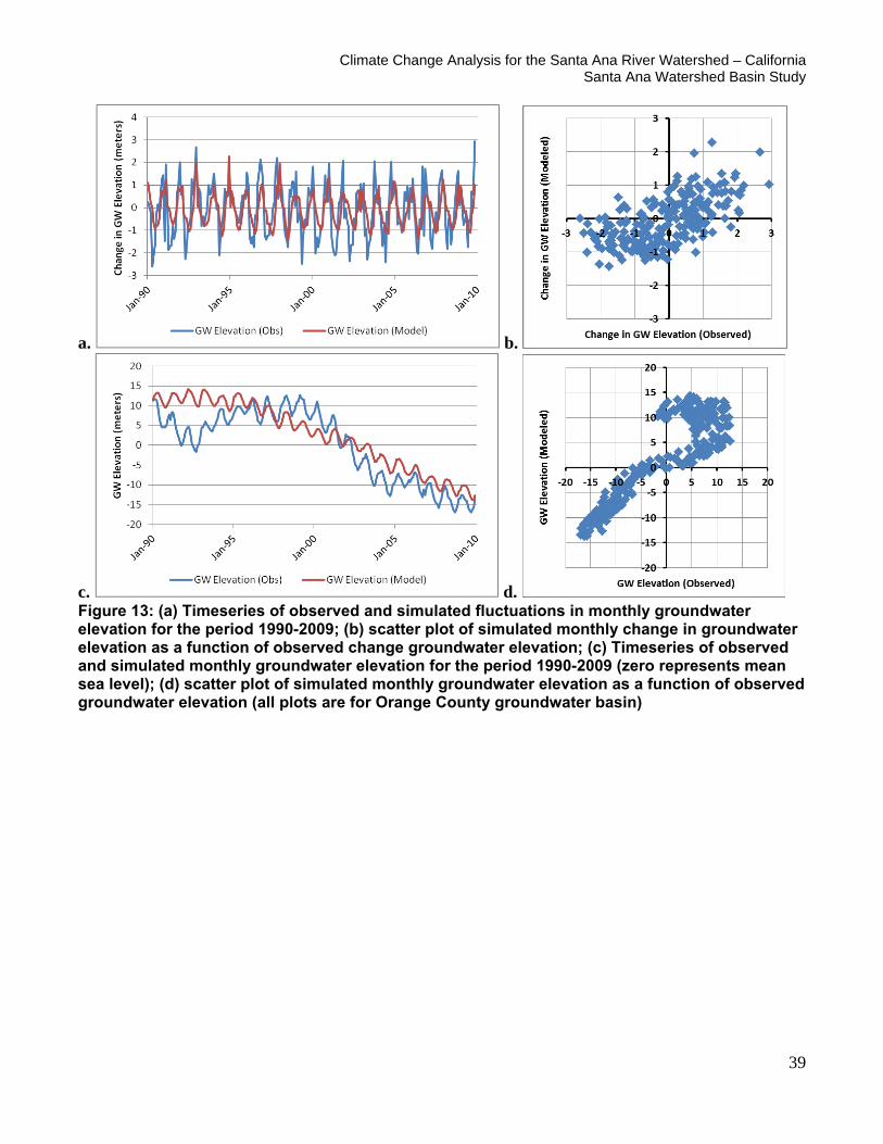
Climate Change Analysis for the Santa Ana River Watershed – California Santa Ana Watershed Basin Study
39
a. b.
c. d. Figure 13: (a) Timeseries of observed and simulated fluctuations in monthly groundwater elevation for the period 1990-2009; (b) scatter plot of simulated monthly change in groundwater elevation as a function of observed change groundwater elevation; (c) Timeseries of observed and simulated monthly groundwater elevation for the period 1990-2009 (zero represents mean sea level); (d) scatter plot of simulated monthly groundwater elevation as a function of observed groundwater elevation (all plots are for Orange County groundwater basin)

Climate Change Analysis for the Santa Ana River Watershed – California Santa Ana Watershed Basin Study
40
Future groundwater availability in the Watershed will depend on future recharge from precipitation, stream seepage, and managed infiltration facilities, as well as future groundwater withdrawals to for municipal, industrial, and agricultural uses. Projected increases in temperature and decreases in precipitation will result in increased water demands and decreased groundwater recharge, respectively. Management actions will be required to protect groundwater resources under projected future climate conditions. Figure 14 illustrates the observed range of basin-averaged groundwater levels in the Orange County groundwater basin for 1990-2009, along with simulated groundwater levels under projected climate conditions. In the absence of groundwater management actions, groundwater levels are projected to decline significantly over the 21st century. It should be noted that projected declines are not constrained by the physical limits of the aquifer; for example, projected declines may exceed the actual amount of usable groundwater in the basin.
Figure 14: Projected groundwater elevations for Orange County for a no action scenario The groundwater screening tool, developed by Reclamation for this Basin Study, can be used to evaluate potential deficiencies in future supplies and to develop sustainable management alternatives. As an example, potential actions to avoid projected water level declines in Orange County are listed below. Each alternative listed will protect against groundwater declines through 2060.
• Reduce M&I demand, gradual reduction of approx. 15% by 2020 (i.e., reduce per capita use from ~175 gallons per day in 2010 to ~150 gallons per day by 2020).
• Increase imports from the Colorado River Aqueduct and State Water Project gradually from ~30,000 acre-ft per year to ~105,000 acre-ft per

Climate Change Analysis for the Santa Ana River Watershed – California Santa Ana Watershed Basin Study
41
year (this may not be feasible due to cost, greenhouse gas emissions, or availability).
• Increase local water supplies by ~75,000 acre-ft per year through recycled water treatment capacity, development of seawater desalination capacity, and increase storm water capture efficiency.
Figures 15, 16, and 17 show the projected groundwater elevations for a no action scenario for the Upper Santa Ana Valley, San Jacinto, and Elsinore respectively. The groundwater screening tool can be used to develop and compare additional management alternatives in order to meet the projected growing demands that are discussed in the next section.
Figure 15: Projected groundwater elevations for Upper Santa Ana Valley for a no action scenario
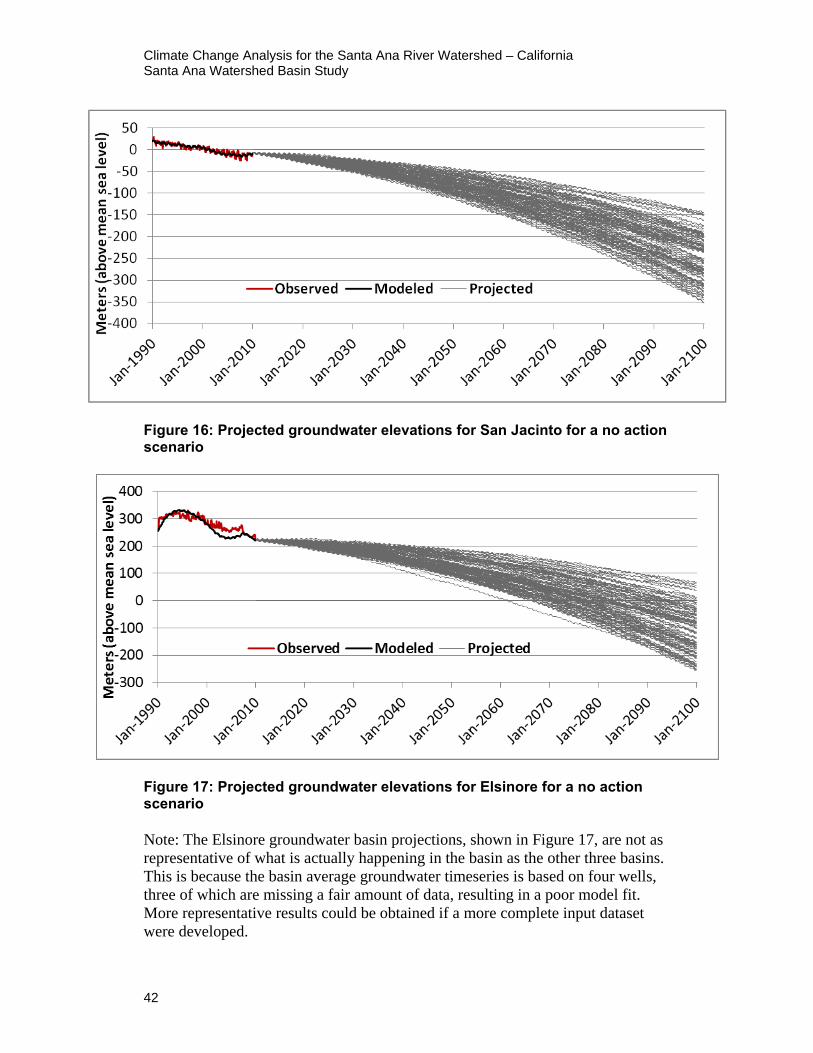
Climate Change Analysis for the Santa Ana River Watershed – California Santa Ana Watershed Basin Study
42
Figure 16: Projected groundwater elevations for San Jacinto for a no action scenario
Figure 17: Projected groundwater elevations for Elsinore for a no action scenario Note: The Elsinore groundwater basin projections, shown in Figure 17, are not as representative of what is actually happening in the basin as the other three basins. This is because the basin average groundwater timeseries is based on four wells, three of which are missing a fair amount of data, resulting in a poor model fit. More representative results could be obtained if a more complete input dataset were developed.
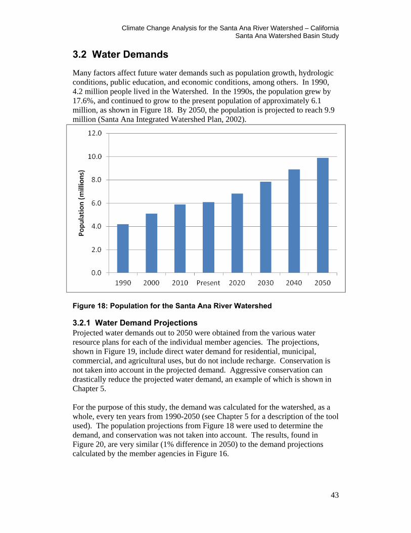
Climate Change Analysis for the Santa Ana River Watershed – California Santa Ana Watershed Basin Study
43
3.2 Water Demands
Many factors affect future water demands such as population growth, hydrologic conditions, public education, and economic conditions, among others. In 1990, 4.2 million people lived in the Watershed. In the 1990s, the population grew by 17.6%, and continued to grow to the present population of approximately 6.1 million, as shown in Figure 18. By 2050, the population is projected to reach 9.9 million (Santa Ana Integrated Watershed Plan, 2002).
Figure 18: Population for the Santa Ana River Watershed
3.2.1 Water Demand Projections Projected water demands out to 2050 were obtained from the various water resource plans for each of the individual member agencies. The projections, shown in Figure 19, include direct water demand for residential, municipal, commercial, and agricultural uses, but do not include recharge. Conservation is not taken into account in the projected demand. Aggressive conservation can drastically reduce the projected water demand, an example of which is shown in Chapter 5. For the purpose of this study, the demand was calculated for the watershed, as a whole, every ten years from 1990-2050 (see Chapter 5 for a description of the tool used). The population projections from Figure 18 were used to determine the demand, and conservation was not taken into account. The results, found in Figure 20, are very similar (1% difference in 2050) to the demand projections calculated by the member agencies in Figure 16.
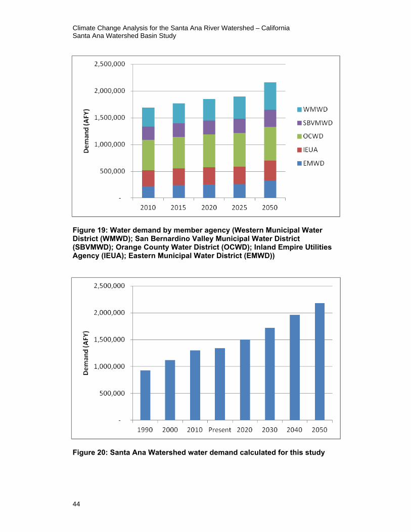
Climate Change Analysis for the Santa Ana River Watershed – California Santa Ana Watershed Basin Study
44
Figure 19: Water demand by member agency (Western Municipal Water District (WMWD); San Bernardino Valley Municipal Water District (SBVMWD); Orange County Water District (OCWD); Inland Empire Utilities Agency (IEUA); Eastern Municipal Water District (EMWD))
Figure 20: Santa Ana Watershed water demand calculated for this study
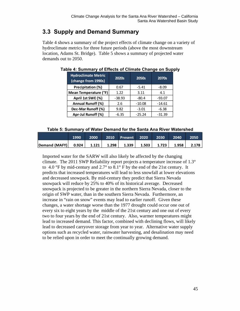
Climate Change Analysis for the Santa Ana River Watershed – California Santa Ana Watershed Basin Study
45
3.3 Supply and Demand Summary
Table 4 shows a summary of the project effects of climate change on a variety of hydroclimate metrics for three future periods (above the most downstream location, Adams St. Bridge). Table 5 shows a summary of projected water demands out to 2050.
Table 4: Summary of Effects of Climate Change on Supply
Table 5: Summary of Water Demand for the Santa Ana River Watershed
Imported water for the SARW will also likely be affected by the changing climate. The 2011 SWP Reliability report projects a temperature increase of 1.3° to 4.0 °F by mid-century and 2.7° to 8.1° F by the end of the 21st century. It predicts that increased temperatures will lead to less snowfall at lower elevations and decreased snowpack. By mid-century they predict that Sierra Nevada snowpack will reduce by 25% to 40% of its historical average. Decreased snowpack is projected to be greater in the northern Sierra Nevada, closer to the origin of SWP water, than in the southern Sierra Nevada. Furthermore, an increase in “rain on snow” events may lead to earlier runoff. Given these changes, a water shortage worse than the 1977 drought could occur one out of every six to eight years by the middle of the 21st century and one out of every two to four years by the end of 21st century. Also, warmer temperatures might lead to increased demand. This factor, combined with declining flows, will likely lead to decreased carryover storage from year to year. Alternative water supply options such as recycled water, rainwater harvesting, and desalination may need to be relied upon in order to meet the continually growing demand.
Hydroclimate Metric (change from 1990s)
2020s 2050s 2070s
Precipitation (%) 0.67 -5.41 -8.09Mean Temperature (°F) 1.22 3.11 4.1
April 1st SWE (%) -38.93 -80.4 -93.07Annual Runoff (%) 2.6 -10.08 -14.61
Dec-Mar Runoff (%) 9.82 -3.01 -6.38Apr-Jul Runoff (%) -6.35 -25.24 -31.39
1990 2000 2010 Present 2020 2030 2040 2050
Demand (MAFY) 0.924 1.121 1.298 1.339 1.503 1.723 1.958 2.178
Climate Change Analysis for the Santa Ana River Watershed – California Santa Ana Watershed Basin Study
46
4.0 Decision Support and Impact Assessment The analyses presented in this chapter were performed using the climate and hydrological projections and models described in Chapter 3.
4.1 Impacts on Recreation in Lake Elsinore
4.1.1 Background Lake Elsinore, shown in Figure 21, is southern California’s largest natural lake and is situated at the bottom of the San Jacinto Watershed. Because Lake Elsinore is a terminal lake, historically fed only by rain and natural runoff, it has been impacted by low lake levels. As the climate continues to change it is likely that these impacts will become more severe. Lake Elsinore is used for recreation and is currently not considered a water supply source. In 2005, Elsinore Valley Municipal Water District (EVMWD) began a two-year pilot project to introduce recycled water into Lake Elsinore to stabilize lake levels. Soon thereafter, a discharge permit was granted to EVMWD by the Santa Ana Regional Water Quality Control Board to allow recycled water to be delivered to the lake. In 2008, a 36-inch-diameter pipeline was constructed to deliver recycled water from EVMWD’s Regional Wastewater Treatment Plant, funded by the State of California Proposition 40 Water Bond and the Lake Elsinore and San Jacinto Watersheds Authority. The project delivers approximately 5 million gallons per day (MGD) of recycled water to Lake Elsinore, and includes repair and retrofit of three local, shallow groundwater wells that deliver approximately 1 MGD. As part of the Basin Study, an analysis was done to determine if these measures would be enough to meet the minimum goal volume of 41,704 acre-ft (elevation 1,240 ft), avoid low lake levels (below 24,659 acre-ft, elevation 1,234 ft), and prevent the lake from drying up altogether (as occurred in the 1930s) under a changing climate.
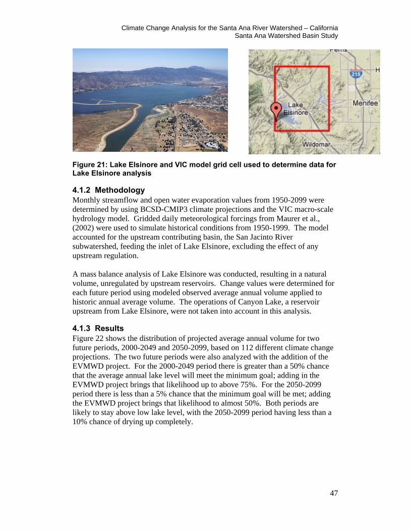
Climate Change Analysis for the Santa Ana River Watershed – California Santa Ana Watershed Basin Study
47
Figure 21: Lake Elsinore and VIC model grid cell used to determine data for Lake Elsinore analysis
4.1.2 Methodology Monthly streamflow and open water evaporation values from 1950-2099 were determined by using BCSD-CMIP3 climate projections and the VIC macro-scale hydrology model. Gridded daily meteorological forcings from Maurer et al., (2002) were used to simulate historical conditions from 1950-1999. The model accounted for the upstream contributing basin, the San Jacinto River subwatershed, feeding the inlet of Lake Elsinore, excluding the effect of any upstream regulation. A mass balance analysis of Lake Elsinore was conducted, resulting in a natural volume, unregulated by upstream reservoirs. Change values were determined for each future period using modeled observed average annual volume applied to historic annual average volume. The operations of Canyon Lake, a reservoir upstream from Lake Elsinore, were not taken into account in this analysis.
4.1.3 Results Figure 22 shows the distribution of projected average annual volume for two future periods, 2000-2049 and 2050-2099, based on 112 different climate change projections. The two future periods were also analyzed with the addition of the EVMWD project. For the 2000-2049 period there is greater than a 50% chance that the average annual lake level will meet the minimum goal; adding in the EVMWD project brings that likelihood up to above 75%. For the 2050-2099 period there is less than a 5% chance that the minimum goal will be met; adding the EVMWD project brings that likelihood to almost 50%. Both periods are likely to stay above low lake level, with the 2050-2099 period having less than a 10% chance of drying up completely.
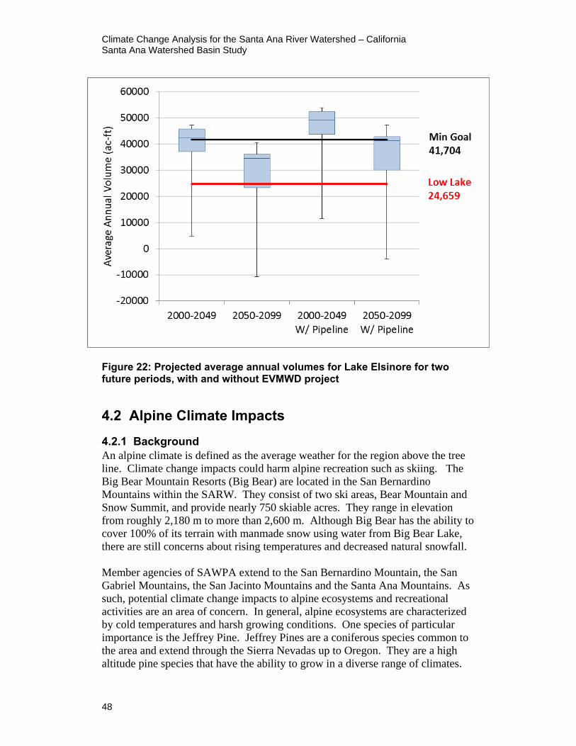
Climate Change Analysis for the Santa Ana River Watershed – California Santa Ana Watershed Basin Study
48
Figure 22: Projected average annual volumes for Lake Elsinore for two future periods, with and without EVMWD project
4.2 Alpine Climate Impacts
4.2.1 Background An alpine climate is defined as the average weather for the region above the tree line. Climate change impacts could harm alpine recreation such as skiing. The Big Bear Mountain Resorts (Big Bear) are located in the San Bernardino Mountains within the SARW. They consist of two ski areas, Bear Mountain and Snow Summit, and provide nearly 750 skiable acres. They range in elevation from roughly 2,180 m to more than 2,600 m. Although Big Bear has the ability to cover 100% of its terrain with manmade snow using water from Big Bear Lake, there are still concerns about rising temperatures and decreased natural snowfall. Member agencies of SAWPA extend to the San Bernardino Mountain, the San Gabriel Mountains, the San Jacinto Mountains and the Santa Ana Mountains. As such, potential climate change impacts to alpine ecosystems and recreational activities are an area of concern. In general, alpine ecosystems are characterized by cold temperatures and harsh growing conditions. One species of particular importance is the Jeffrey Pine. Jeffrey Pines are a coniferous species common to the area and extend through the Sierra Nevadas up to Oregon. They are a high altitude pine species that have the ability to grow in a diverse range of climates.

Climate Change Analysis for the Santa Ana River Watershed – California Santa Ana Watershed Basin Study
49
They can do well in harsh settings and infertile sites because they require a shorter growing season than some other species (Moore, 2006).
4.2.2 Methodology Impacts to skiing near Big Bear Lake were analyzed by considering projected changes for April 1st SWE. April 1st SWE values from 1950 to 2099 were generated for 112 CMIP3 climate projections using the VIC model forced with downscaled (BCSD) climate variables. Each climate projection consists of 1/8° x 1/8° degree (~12 km x 12km) grid cell daily forcings. For this analysis, the locations of the Bear Mountain and Snow Summit ski areas were mapped to the single grid cell that contained them. Results shown in Section 4.2.3 summarize the median change (taken from the 112 projections) in April 1st SWE compared to the 1990s. For comparison, results were also summarized from a study of climate change impacts in California by Hayhoe et al. (2004). They used climate forcing data generated with two GCMs of low (Parallel Climate Model, PCM) and medium (Hadley Center Climate Model version 3, HadCM3) sensitivity, forced using two emissions scenarios, one lower (B1) and one higher (A1fi). SWE results were generated using the VIC model forced with the BCSD temperature and precipitation. Results are provided in Section 4.2.3 on a statewide basis grouped by elevation. Quantitative analysis of ecosystem impacts was not conducted as part of this work. Rather a literature review of existing climate change impact studies was conducted and the relevant findings are provided here.
4.2.3 Results
Recreation at Big Bear It is likely that future snowpack at Big Bear will be significantly less than what is currently normal and accumulated snowpack will remain on the ground for a shorter season. Figures 23 and 24 illustrate future changes in April 1st SWE. Projected declines are between 30% and 40% by the 2020s, and are generally projected to be greater than 70% by the 2070s. These changes are largely a result of increased winter temperatures and potential declines in winter precipitation. Warmer temperatures will result in a delayed onset of the ski season, as well as earlier spring melting. Future precipitation is much more uncertain but many projections show decreased winter precipitation. Lower altitudes will likely be the most sensitive to increased temperature because small temperature changes can result in precipitation falling as rain rather than snow. Hayhoe et al. (2004) note that reductions in SWE are most pronounced below 3,000 m where roughly 80% of California’s snowpack storage currently occurs. The Bear Mountain and Snow Summit ski areas both fall between roughly 2,100 and 2,600 m, making them vulnerable to increased temperatures.

Climate Change Analysis for the Santa Ana River Watershed – California Santa Ana Watershed Basin Study
50
While there is general consensus for a projected decrease in snowpack, it is also important to note that there is significant variability between climate projections. For example, the low sensitivity, low emissions scenario in Figure 24 projects only a 20% decrease in snowpack by 2070, while the other scenarios as well as the median, shown in Figure 23, project a greater than 70% decrease. Also, the grid resolution for both methodologies is 1/8° which is much larger than either ski area. As such, results include surrounding areas that are at lower elevations and beyond ski area itself. However, the overall findings in Figures 23 and 24 are consistent.
Figure 23: Median percent change (from 112 climate projections) in April 1st SWE for the grid cells containing the Bear Mountain and Snow Summit ski areas
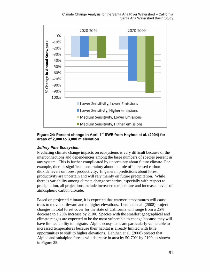
Climate Change Analysis for the Santa Ana River Watershed – California Santa Ana Watershed Basin Study
51
Figure 24: Percent change in April 1st SWE from Hayhoe et al. (2004) for areas of 2,000 to 3,000 m elevation
Jeffrey Pine Ecosystem Predicting climate change impacts on ecosystems is very difficult because of the interconnections and dependencies among the large numbers of species present in any system. This is further complicated by uncertainty about future climate. For example, there is significant uncertainty about the role of increased carbon dioxide levels on forest productivity. In general, predictions about forest productivity are uncertain and will rely mainly on future precipitation. While there is variability among climate change scenarios, especially with respect to precipitation, all projections include increased temperature and increased levels of atmospheric carbon dioxide. Based on projected climate, it is expected that warmer temperatures will cause trees to move northward and to higher elevations. Lenihan et al. (2008) project changes in total forest cover for the state of California will range from a 25% decrease to a 23% increase by 2100. Species with the smallest geographical and climate ranges are expected to be the most vulnerable to change because they will have limited ability to migrate. Alpine ecosystems are particularly vulnerable to increased temperatures because their habitat is already limited with little opportunities to shift to higher elevations. Lenihan et al. (2008) project that Alpine and subalpine forests will decrease in area by 50-70% by 2100, as shown in Figure 25.
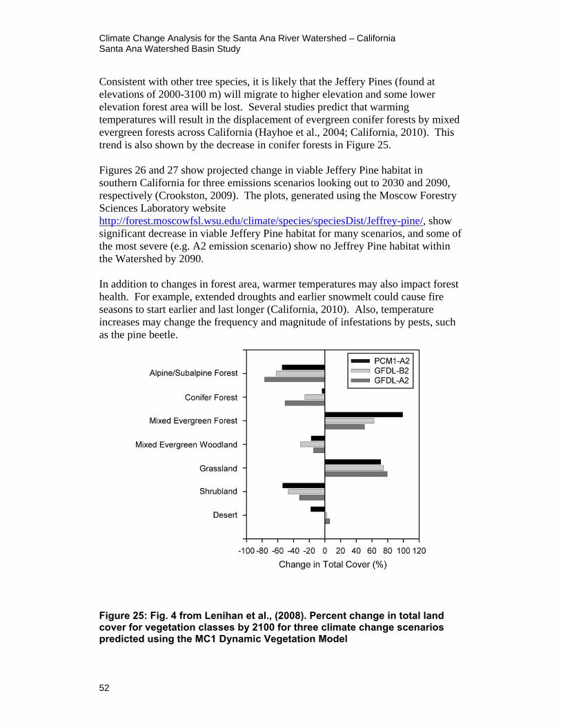
Climate Change Analysis for the Santa Ana River Watershed – California Santa Ana Watershed Basin Study
52
Consistent with other tree species, it is likely that the Jeffery Pines (found at elevations of 2000-3100 m) will migrate to higher elevation and some lower elevation forest area will be lost. Several studies predict that warming temperatures will result in the displacement of evergreen conifer forests by mixed evergreen forests across California (Hayhoe et al., 2004; California, 2010). This trend is also shown by the decrease in conifer forests in Figure 25. Figures 26 and 27 show projected change in viable Jeffery Pine habitat in southern California for three emissions scenarios looking out to 2030 and 2090, respectively (Crookston, 2009). The plots, generated using the Moscow Forestry Sciences Laboratory website http://forest.moscowfsl.wsu.edu/climate/species/speciesDist/Jeffrey-pine/, show significant decrease in viable Jeffery Pine habitat for many scenarios, and some of the most severe (e.g. A2 emission scenario) show no Jeffrey Pine habitat within the Watershed by 2090. In addition to changes in forest area, warmer temperatures may also impact forest health. For example, extended droughts and earlier snowmelt could cause fire seasons to start earlier and last longer (California, 2010). Also, temperature increases may change the frequency and magnitude of infestations by pests, such as the pine beetle. Figure 25: Fig. 4 from Lenihan et al., (2008). Percent change in total land cover for vegetation classes by 2100 for three climate change scenarios predicted using the MC1 Dynamic Vegetation Model

Climate Change Analysis for the Santa Ana River Watershed – California Santa Ana Watershed Basin Study
53
Figure 26: Viability scores for Jeffery Pine currently and for three future projections for 2030
Figure 27: Viability scores for Jeffery Pine currently and for three future projections for 2090 Source: http://forest.moscowfsl.wsu.edu/climate/species/speciesDist/Jeffrey-pine/
Climate Change Analysis for the Santa Ana River Watershed – California Santa Ana Watershed Basin Study
54
4.3 Extreme Temperature Impacts
4.3.1 Background There is no standard definition of an extreme heat event, commonly known as a “heat wave.” It is most commonly defined as a period with more than three consecutive days of maximum temperatures at or above 90°F. However, temperature is only one component of heat, which also depends on humidity, wind speed and radiant load. Climate change is resulting in more frequent and severe heat waves (Dia, 2011). The increased heat could lead to additional air pollution in urban areas, bringing increased health risks. In 2007, the IPCC concluded that “hot extremes” and “heat waves” are very likely (>90% probability of occurrence) to increase as our climate continues to change. This predicted temperature increase is particularly pronounced for night temperatures, resulting in reduced night-time relief from the heat. These changing weather conditions are a growing concern for individuals and communities in the Watershed.
4.3.2 Methodology Daily maximum temperature values came from the BCSD-CMIP3 archive for 112 climate projections. Each projection has 1/8° x 1/8° (~12 km x 12 km) grid cell daily forcings that start on January 1, 1950 and run through December 31, 2099. For this analysis, the location of each city was matched to the single VIC grid cell that contains it. The data was analyzed and days with maximum temperatures over 95°F were considered to contribute to the results, found in Section 4.3.3, which summarize temperature trends for all 112 projections from 1950 to 2099 for the selected grid cell.
4.3.3 Results Figure 28 shows the distribution of the annual number of days above 95°F from 1950-2099 for each of the cities (Anaheim, Riverside, and Big Bear City) for all 112 climate projections. As shown here, there is a clear, increasing trend in the number of days above 95°F for all three locations, with Riverside in the lead, followed by Anaheim. Big Bear City has the least number of days with a median of zero for all years prior to about 2030. The shaded area in Figure 28 shows the range of the 112 climate projections and demonstrates a large spread in projected results. Table 6 summarizes the median number of days above 95°F for each location for the historical time period (1951-1999) and three 30-year future time periods centered around 2020, 2050 and 2070. As shown in Table 6, the number of days increases for all stations advancing into the future. Changes are quite significant; for example, the median value for Anaheim quadrupled from 4 to 16 days between the historical time period and 2070. Similarly, the median value for Riverside nearly doubled between the historical time period and 2070 going from 43 to 82 days.
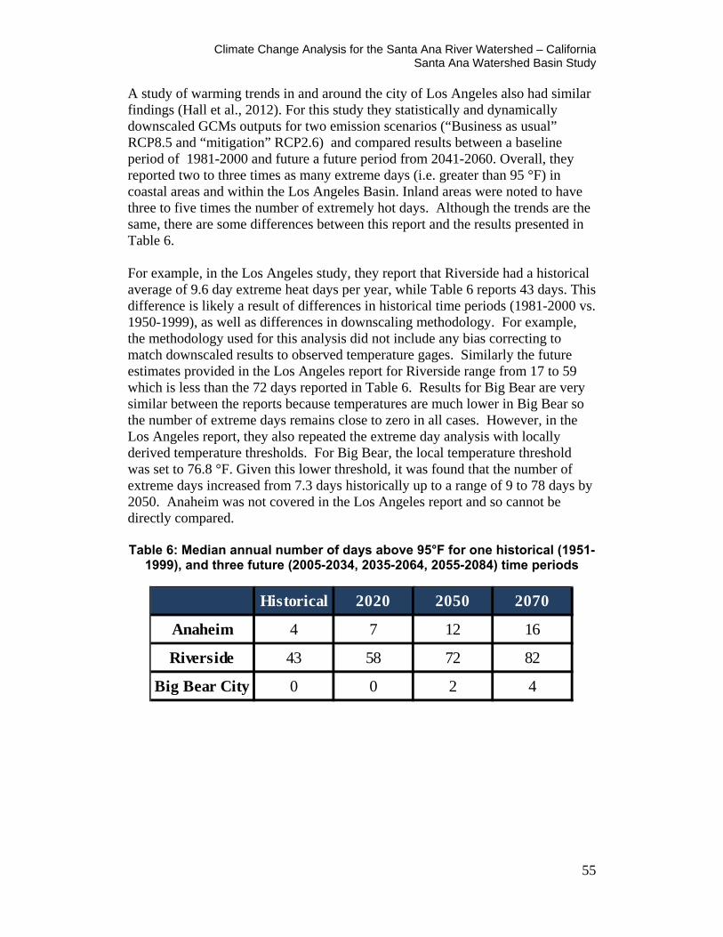
Climate Change Analysis for the Santa Ana River Watershed – California Santa Ana Watershed Basin Study
55
A study of warming trends in and around the city of Los Angeles also had similar findings (Hall et al., 2012). For this study they statistically and dynamically downscaled GCMs outputs for two emission scenarios (“Business as usual” RCP8.5 and “mitigation” RCP2.6) and compared results between a baseline period of 1981-2000 and future a future period from 2041-2060. Overall, they reported two to three times as many extreme days (i.e. greater than 95 °F) in coastal areas and within the Los Angeles Basin. Inland areas were noted to have three to five times the number of extremely hot days. Although the trends are the same, there are some differences between this report and the results presented in Table 6. For example, in the Los Angeles study, they report that Riverside had a historical average of 9.6 day extreme heat days per year, while Table 6 reports 43 days. This difference is likely a result of differences in historical time periods (1981-2000 vs. 1950-1999), as well as differences in downscaling methodology. For example, the methodology used for this analysis did not include any bias correcting to match downscaled results to observed temperature gages. Similarly the future estimates provided in the Los Angeles report for Riverside range from 17 to 59 which is less than the 72 days reported in Table 6. Results for Big Bear are very similar between the reports because temperatures are much lower in Big Bear so the number of extreme days remains close to zero in all cases. However, in the Los Angeles report, they also repeated the extreme day analysis with locally derived temperature thresholds. For Big Bear, the local temperature threshold was set to 76.8 °F. Given this lower threshold, it was found that the number of extreme days increased from 7.3 days historically up to a range of 9 to 78 days by 2050. Anaheim was not covered in the Los Angeles report and so cannot be directly compared. Table 6: Median annual number of days above 95°F for one historical (1951-
1999), and three future (2005-2034, 2035-2064, 2055-2084) time periods
Historical 2020 2050 2070
Anaheim 4 7 12 16
Riverside 43 58 72 82
Big Bear City 0 0 2 4
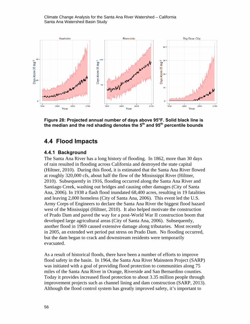
Climate Change Analysis for the Santa Ana River Watershed – California Santa Ana Watershed Basin Study
56
Figure 28: Projected annual number of days above 95°F. Solid black line is the median and the red shading denotes the 5th and 95th percentile bounds
4.4 Flood Impacts
4.4.1 Background The Santa Ana River has a long history of flooding. In 1862, more than 30 days of rain resulted in flooding across California and destroyed the state capital (Hiltner, 2010). During this flood, it is estimated that the Santa Ana River flowed at roughly 320,000 cfs, about half the flow of the Mississippi River (Hiltner, 2010). Subsequently in 1916, flooding occurred along the Santa Ana River and Santiago Creek, washing out bridges and causing other damages (City of Santa Ana, 2006). In 1938 a flash flood inundated 68,400 acres, resulting in 19 fatalities and leaving 2,000 homeless (City of Santa Ana, 2006). This event led the U.S. Army Corps of Engineers to declare the Santa Ana River the biggest flood hazard west of the Mississippi (Hiltner, 2010). It also helped motivate the construction of Prado Dam and paved the way for a post-World War II construction boom that developed large agricultural areas (City of Santa Ana, 2006). Subsequently, another flood in 1969 caused extensive damage along tributaries. Most recently in 2005, an extended wet period put stress on Prado Dam. No flooding occurred, but the dam began to crack and downstream residents were temporarily evacuated. As a result of historical floods, there have been a number of efforts to improve flood safety in the basin. In 1964, the Santa Ana River Mainstem Project (SARP) was initiated with a goal of providing flood protection to communities along 75 miles of the Santa Ana River in Orange, Riverside and San Bernardino counties. Today it provides increased flood protection to about 3.35 million people through improvement projects such as channel lining and dam construction (SARP, 2013). Although the flood control system has greatly improved safety, it’s important to
Climate Change Analysis for the Santa Ana River Watershed – California Santa Ana Watershed Basin Study
57
note that increased development in the area has also increased impervious area and decreased the effectiveness of existing infrastructure. Generally, the goal of flood frequency analysis is to determine the probability of occurrence for a range of flood values. Often this is expressed in terms of return periods (equal to the inverse of the threshold exceedance probability). If the probability of a given flood magnitude occurring in a given year is 1%, then the return interval is equal to 100-years (assuming every year is an independent sample from all years and that events are equally likely). There are two main approaches to flood frequency analysis. The extreme value approach uses historical flood data to generate a probability distribution that can be used to predict the flood magnitude for any number of return intervals. Alternatively, flood process can be modeled directly using physically-based hydrodynamic models driven by meteorological forcings. For this analysis we combine both approaches; first we simulate floods using a physically based hydrologic model, then we fit an extreme value distribution to the results. Extreme value functions are designed to capture the distribution of extremes drawn from other distributions. Pearson Type III and Generalized Extreme Value (GEV) are two of the most commonly used distributions. The Gumbel and Weibul distributions are special cases of the GEV distribution that are commonly applied in hydrology. For this work we use the Log Pearson Type III distribution following the standard United States Government methodology presented in Bulletin 17B, “Guidelines for Determining Flood Flow Frequency” (Bulletin 17B, 1982). Once an extreme value function has been chosen, the next task is to fit it to the observed data. There are three main approaches: plotting positions, method of moments, and maximum likelihood. Plotting positions is the simplest approach; it’s based on visualizing the observed data and fitting a distribution visually or by minimizing errors (e.g. using least squares fitting). Although this method is very straightforward, it is not very commonly used because it is problematic when dealing with limited data. Also, when using least squares to fit, the errors are minimized between sample values and distribution values, but the error that should in fact be considered is frequency not value (FEMA, 2007). To improve upon this, the method of moments fits distributions using the various moments of the observed data (e.g. mean, variance, skew, kurtosis) rather than the values themselves. For example, one can simply compute sample moments and distribution moments and solve for distribution parameters. This approach can also be difficult, because simple moments may not exist for a given distribution and higher order moments may be limited by sample size (FEMA, 2007). Probability-weighted moments and linear moments (L-Moments) can address these issues (Hosking and Wallis, 1997). Finally, the maximum likelihood approach calculates the likelihood of a sample given the assumed distribution. Parameters are determined by trying to maximize the likelihood or often (log

Climate Change Analysis for the Santa Ana River Watershed – California Santa Ana Watershed Basin Study
58
likelihood) for a chosen distribution. Once again following the standard methodology recommended in Bulletin 17B, we will fit distributions using the methods of moments for this analysis. Before applying flood frequency analysis, it is important to understand key underlying assumptions. All extreme value distributions assume that annual max floods are independent samples from a population. Also the distribution approach assumes point data. If data is available from multiple sites, regional frequency analysis can be used to improve parameter estimation. Finally, most extreme value approaches, including the methodology used here, assume that the distribution that is fit to the observed data remains stationary throughout time. This assumption can be problematic in the face of changing climate in which we might expect increased frequency of extreme events. To address this issue, a number of studies have explored the use of non-stationary extreme value distributions in which distribution parameters are allowed to vary as a function of covariates such as time, precipitation or temperature (Katz and Naveau, 2002; Graffis and Stedinger, 2007). For this study, we fit the traditional stationary models. However, we do account for climate change through the physical modeling step by applying non-stationary climate forcings to simulate future floods.
4.4.2 Methodology As previously noted, for this analysis we used a combined physical and statistical modeling approach. First, floods are modeled using the VIC physical model forced with climate data from 112 climate simulations. Next, Log Pearson distributions are fit to the annual maximum flood values for each simulation for a range of historical and future time periods. We consider three locations along the Santa Ana: Prado Dam, Seven Oaks Dam, and the Adams Street gage near the river outlet. Three 30-year periods are considered centered around: 2020, 2050 and 2070. The historical period spans 50 years from 1950 to 1999. Annual maximum one-day flood values are calculated from the VIC outputs for each of the 112 150-year simulations. Flood frequencies are estimated following the standard United States Government method outlined in Bulletin 17-B. For each analysis time period (one historical and three 30-year futures) and climate scenario, a Log Pearson III distribution is fit to the annual maximum values using the L-moments approach. Note that each time period is treated separately. For example, each future period will have 30 values with which to fit the distribution. Using the parameters for the Log-Pearson III distributions, the 200-year return period flow values are estimated for every climate simulation and analysis period. The 200-year storm was used in order to fill the requirements set forth in the California Department of Water Resources’ Climate Change Handbook for Regional Water Planning (Appendix B). The distribution is also used to calculate the return period for the median historical 200-year flood for each climate simulation and future time period.
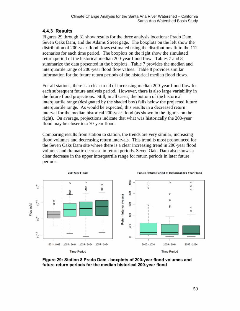
Climate Change Analysis for the Santa Ana River Watershed – California Santa Ana Watershed Basin Study
59
4.4.3 Results Figures 29 through 31 show results for the three analysis locations: Prado Dam, Seven Oaks Dam, and the Adams Street gage. The boxplots on the left show the distribution of 200-year flood flows estimated using the distributions fit to the 112 scenarios for each time period. The boxplots on the right show the simulated return period of the historical median 200-year flood flow. Tables 7 and 8 summarize the data presented in the boxplots. Table 7 provides the median and interquartile range of 200-year flood flow values. Table 8 provides similar information for the future return periods of the historical median flood flows. For all stations, there is a clear trend of increasing median 200-year flood flow for each subsequent future analysis period. However, there is also large variability in the future flood projections. Still, in all cases, the bottom of the historical interquartile range (designated by the shaded box) falls below the projected future interquartile range. As would be expected, this results in a decreased return interval for the median historical 200-year flood (as shown in the figures on the right). On average, projections indicate that what was historically the 200-year flood may be closer to a 70-year flood. Comparing results from station to station, the trends are very similar, increasing flood volumes and decreasing return intervals. This trend is most pronounced for the Seven Oaks Dam site where there is a clear increasing trend in 200-year flood volumes and dramatic decrease in return periods. Seven Oaks Dam also shows a clear decrease in the upper interquartile range for return periods in later future periods.
Figure 29: Station 8 Prado Dam - boxplots of 200-year flood volumes and future return periods for the median historical 200-year flood
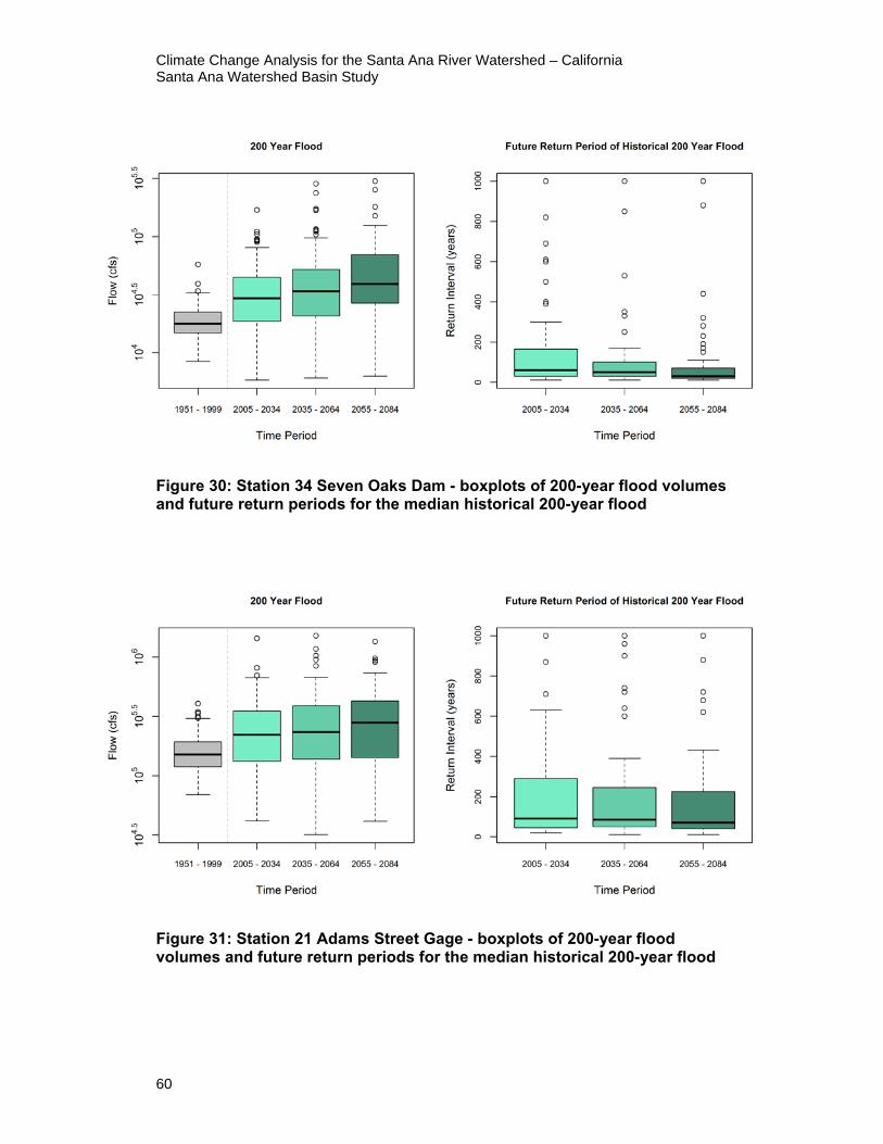
Climate Change Analysis for the Santa Ana River Watershed – California Santa Ana Watershed Basin Study
60
Figure 30: Station 34 Seven Oaks Dam - boxplots of 200-year flood volumes and future return periods for the median historical 200-year flood
Figure 31: Station 21 Adams Street Gage - boxplots of 200-year flood volumes and future return periods for the median historical 200-year flood
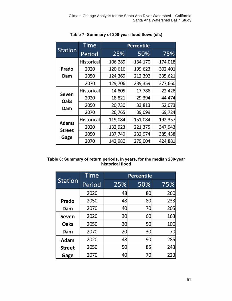
Climate Change Analysis for the Santa Ana River Watershed – California Santa Ana Watershed Basin Study
61
Table 7: Summary of 200-year flood flows (cfs)
Table 8: Summary of return periods, in years, for the median 200-year historical flood
25% 50% 75%Historical 106,289 134,170 174,018
2020 120,616 199,623 302,4012050 124,369 212,392 335,6212070 129,706 239,359 377,660
Historical 14,805 17,786 22,4282020 18,821 29,394 44,4742050 20,730 33,813 52,0732070 26,765 39,099 69,724
Historical 119,084 151,084 192,3572020 132,923 221,375 347,9432050 137,749 232,974 385,4382070 142,980 279,004 424,881
StationTime
PeriodPercentile
Prado Dam
Seven Oaks Dam
Adams Street Gage
25% 50% 75%2020 48 80 2602050 48 80 2332070 40 70 2052020 30 60 1632050 30 50 1002070 20 30 702020 48 90 2852050 50 85 2432070 40 70 223
PercentileStation
Time Period
Prado Dam
Seven Oaks Dam
Adam Street Gage
Climate Change Analysis for the Santa Ana River Watershed – California Santa Ana Watershed Basin Study
62
Results from this analysis indicate increased risk of flooding in the future. This is demonstrated by increased 200-year flood magnitudes as well as decreased recurrence intervals for what was historically considered a 200-year flood. While these results show clear trends, it is also important to note that there is large variability between climate simulations. For the purposes of this analysis, it is assumed that all future scenarios are equally likely. Variability in the results reflects large underlying uncertainties with GCM outputs and downscaling methodologies. Additionally, the quality of results is necessarily limited by the ability of the VIC model to accurately generate flood flows from forcing data. While these constraints are acknowledged, it should be noted that this analysis follows standard methodologies and utilizes the best available input data.
4.5 Sea Level Rise Impacts
4.5.1 Background Climate change will contribute to global sea level rise (SLR) through melting of glaciers and ice caps and thermal expansion of ocean waters, both of which increase the volume of water in the oceans. Regional SLR may be higher or lower than global SLR due to effects of regional ocean and atmospheric circulation. California’s 2,000 miles of coastline has experienced just under eight inches of sea level rise over the past decade (Cayan et al., 2009), a number that is likely to increase drastically as the climate continues to change. Critical infrastructure, such as roads, hospitals, schools, emergency facilities, wastewater treatment plants, power plants, and more will also be at increased risk of inundation, as are vast areas of wetlands and other natural ecosystems. Flooding and erosion already pose a threat to communities along the California coast and there is compelling evidence that these risks will increase in the future. In areas where the coast erodes easily, sea level rise will likely accelerate shoreline recession due to erosion. Erosion of some barrier dunes may expose previously protected areas to flooding.
4.5.2 Methodology Orange County Water District (OCWD) conducted a study to evaluate the potential effects of projected sea level rise on coastal Orange County groundwater conditions. Two locations were selected near the Talbert and Alamitos injection barriers, shown in Figure 32. Projected sea level rise scenarios were developed by the California Climate Change Center (Cayan et al., 2009). For this analysis, the moderate projected sea level rise along the California coast was used. The projected time horizon or year is not critical for the model runs (described below), but rather just the sea level rise amount. Therefore, to bracket the entire range of projected moderate case sea
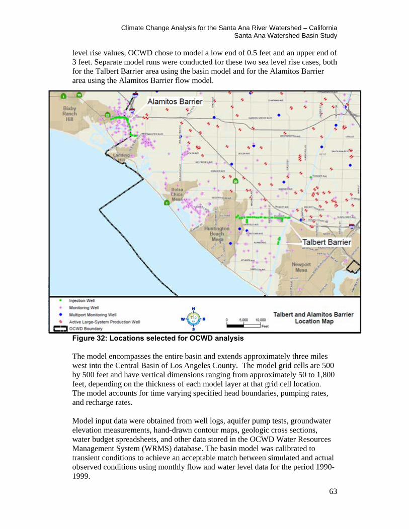
Climate Change Analysis for the Santa Ana River Watershed – California Santa Ana Watershed Basin Study
63
level rise values, OCWD chose to model a low end of 0.5 feet and an upper end of 3 feet. Separate model runs were conducted for these two sea level rise cases, both for the Talbert Barrier area using the basin model and for the Alamitos Barrier area using the Alamitos Barrier flow model.
Figure 32: Locations selected for OCWD analysis The model encompasses the entire basin and extends approximately three miles west into the Central Basin of Los Angeles County. The model grid cells are 500 by 500 feet and have vertical dimensions ranging from approximately 50 to 1,800 feet, depending on the thickness of each model layer at that grid cell location. The model accounts for time varying specified head boundaries, pumping rates, and recharge rates. Model input data were obtained from well logs, aquifer pump tests, groundwater elevation measurements, hand-drawn contour maps, geologic cross sections, water budget spreadsheets, and other data stored in the OCWD Water Resources Management System (WRMS) database. The basin model was calibrated to transient conditions to achieve an acceptable match between simulated and actual observed conditions using monthly flow and water level data for the period 1990-1999.
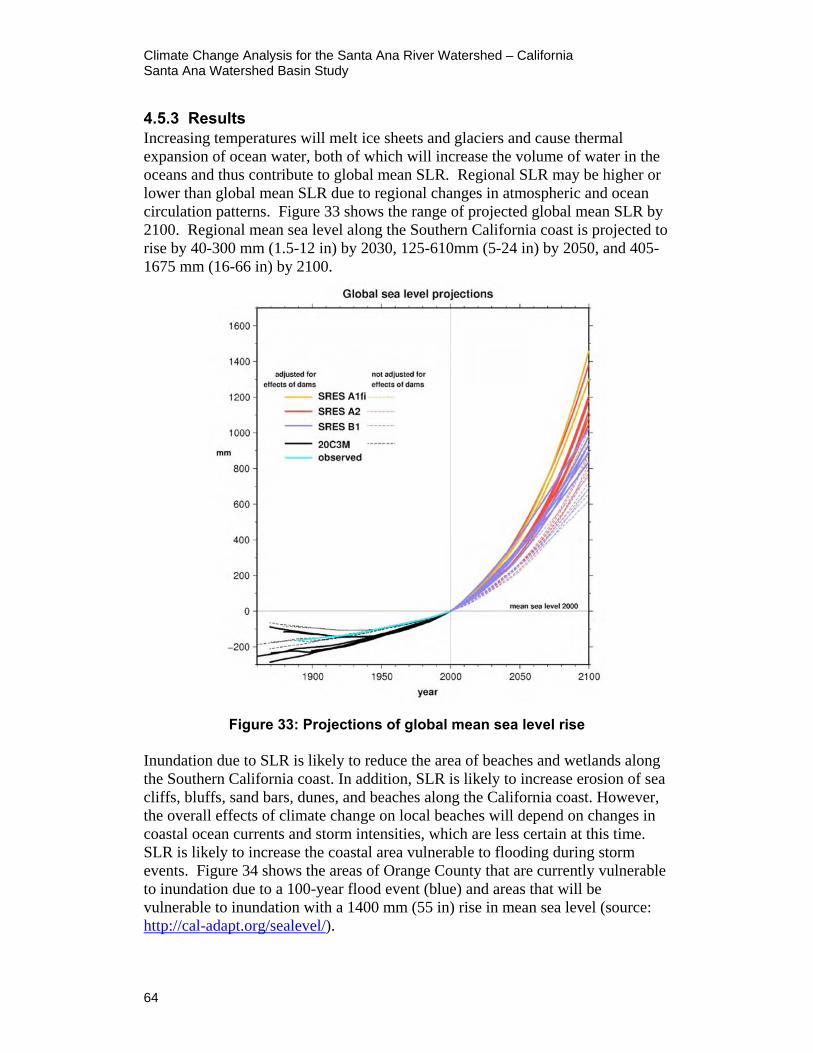
Climate Change Analysis for the Santa Ana River Watershed – California Santa Ana Watershed Basin Study
64
4.5.3 Results Increasing temperatures will melt ice sheets and glaciers and cause thermal expansion of ocean water, both of which will increase the volume of water in the oceans and thus contribute to global mean SLR. Regional SLR may be higher or lower than global mean SLR due to regional changes in atmospheric and ocean circulation patterns. Figure 33 shows the range of projected global mean SLR by 2100. Regional mean sea level along the Southern California coast is projected to rise by 40-300 mm (1.5-12 in) by 2030, 125-610mm (5-24 in) by 2050, and 405-1675 mm (16-66 in) by 2100.
Figure 33: Projections of global mean sea level rise Inundation due to SLR is likely to reduce the area of beaches and wetlands along the Southern California coast. In addition, SLR is likely to increase erosion of sea cliffs, bluffs, sand bars, dunes, and beaches along the California coast. However, the overall effects of climate change on local beaches will depend on changes in coastal ocean currents and storm intensities, which are less certain at this time. SLR is likely to increase the coastal area vulnerable to flooding during storm events. Figure 34 shows the areas of Orange County that are currently vulnerable to inundation due to a 100-year flood event (blue) and areas that will be vulnerable to inundation with a 1400 mm (55 in) rise in mean sea level (source: http://cal-adapt.org/sealevel/).
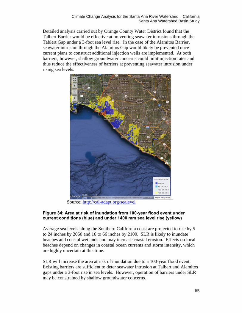
Climate Change Analysis for the Santa Ana River Watershed – California Santa Ana Watershed Basin Study
65
Detailed analysis carried out by Orange County Water District found that the Talbert Barrier would be effective at preventing seawater intrusions through the Tablert Gap under a 3-foot sea level rise. In the case of the Alamitos Barrier, seawater intrusion through the Alamitos Gap would likely be prevented once current plans to construct additional injection wells are implemented. At both barriers, however, shallow groundwater concerns could limit injection rates and thus reduce the effectiveness of barriers at preventing seawater intrusion under rising sea levels.
Figure 34: Area at risk of inundation from 100-year flood event under current conditions (blue) and under 1400 mm sea level rise (yellow) Average sea levels along the Southern California coast are projected to rise by 5 to 24 inches by 2050 and 16 to 66 inches by 2100. SLR is likely to inundate beaches and coastal wetlands and may increase coastal erosion. Effects on local beaches depend on changes in coastal ocean currents and storm intensity, which are highly uncertain at this time. SLR will increase the area at risk of inundation due to a 100-year flood event. Existing barriers are sufficient to deter seawater intrusion at Talbert and Alamitos gaps under a 3-foot rise in sea levels. However, operation of barriers under SLR may be constrained by shallow groundwater concerns.
Source: http://cal-adapt.org/sealevel

Climate Change Analysis for the Santa Ana River Watershed – California Santa Ana Watershed Basin Study
66
4.6 Decision Support and Impact Assessment Summary
A set of frequently asked questions (FAQs) were answered using the previous analyses. Those questions and the key findings are summarized below. Will surface water supply decrease?
• Annual surface water is likely to decrease over future periods. • Precipitation shows somewhat long-term decreasing trends. • Temperature will increase, which is likely to cause increased water
demand and reservoir evaporation. • April 1st SWE will decrease.
Will groundwater availability be reduced?
• Groundwater currently provides approximately 54% of total water supply in an average year, and groundwater use is projected to increase over the next 20 years.
• Projected decreases in precipitation and increases in temperature will decrease natural recharge throughout the basin.
• Management actions such as reducing municipal and industrial water demands or increasing trans-basin water imports and recharge will be required in order to maintain current groundwater levels.
• A basin-scale groundwater screening tool was developed to facilitate analysis of basin-scale effects of conservation, increasing imported supply, changing agricultural land use, and other factors on basin-scale groundwater conditions.
Is Lake Elsinore in danger of drying up?
• Lake Elsinore has less than a 10% chance of drying up (2000-2099). • In the 2000-2049 period, Lake Elsinore has a greater than 75% chance of
meeting the minimum elevation goal of 1,240 ft. • In the future period 2050-2099, Lake Elsinore has less than a 50% chance
of meeting the minimum elevation goal of 1,240 ft. • There is less than a 25% chance that Lake Elsinore will drop below low
lake levels (1,234 ft) in either period. • The Elsinore Valley Municipal Water District (EVMWD) project does aid
in stabilizing lake levels; however, for the period 2050-2099 additional measures will likely be required to meet the minimum elevation goal of 1,240 ft.
Climate Change Analysis for the Santa Ana River Watershed – California Santa Ana Watershed Basin Study
67
Will the region continue to support an alpine climate and how will the Jeffrey Pine ecosystem be impacted?
• Warmer temperatures will likely cause Jeffrey pines to move to higher elevations and may decrease their total habitat.
• Forest health may also be influenced by changes in the magnitude and frequency of wildfires or infestations.
• Alpine ecosystems are vulnerable to climate change because they have little ability to expand to higher elevations.
• Across the State it is projected that alpine forests will decrease in area by 50-70% by 2100.
Will skiing at Big Bear Mountain Resorts be sustained?
• Simulations indicate significant decreases in April 1st snowpack that amplify throughout the 21st century.
• Warmer temperatures will also result in a delayed onset and shortened ski season.
• Lower elevations are most vulnerable to increasing temperatures. • Both Big Bear Mountain Resorts lie below 3,000 m and are projected to
experience declining snowpack that could exceed 70% by 2070.
How many additional days over 95°F are expected in Anaheim, Riverside and Big Bear City?
• All the climate projections demonstrate clear increasing temperature trends.
• Increasing temperatures will result in a greater number of days above 95°F in the future.
• The number of days above 95°F gets progressively larger for all cities advancing into the future.
• By 2070 it is projected that the number of days above 95°F will quadruple in Anaheim (4 to 16 days) and nearly double in Riverside (43 to 82 days). The number of days above 95°F at Big Bear City is projected to increase from 0 days historically to 4 days in 2070.
Will floods become more severe and threaten flood infrastructure?
• Simulations indicate a significant increase in flow for 200-year storm events in the future.
• The likelihood of experiencing what was historically a 200-year event will nearly double (i.e. the 200-year historical event is likely to be closer to a 100-year event in the future).
• Findings indicate an increased risk of severe floods in the future, though there is large variability between climate simulations.
Climate Change Analysis for the Santa Ana River Watershed – California Santa Ana Watershed Basin Study
68
How will climate change and sea level rise affect coastal communities and beaches?
• Climate change will contribute to global sea level rise (SLR) through melting of glaciers and ice caps and thermal expansion of ocean waters, both of which increase the volume of water in the oceans.
• Regional SLR may be higher or lower than global SLR due to effects of regional ocean and atmospheric circulation.
• Average sea levels along the Southern California coast are projected to rise by 5 to 24 inches by 2050 and 16 to 66 inches by 2100.
• SLR is likely to inundate beaches and coastal wetlands and may increase coastal erosion. Effects on local beaches depend on changes in coastal ocean currents and storm intensity, which are highly uncertain at this time.
• SLR will increase the area at risk of inundation due to a 100-year flood event.
• Existing barriers are sufficient to deter seawater intrusion at Talbert and Alamitos gaps under a 3-foot rise in sea levels. However, operation of barriers under SLR may be constrained by shallow groundwater concerns.
In order to adapt to the impacts of climate change described in this chapter, water managers need tools that enable them to make informed decisions. Reclamation has developed a tool, the Greenhouse Gas (GHG) Emissions Calculator, which can be used to inform adaptive strategies. This tool was used to conduct a demand management case study for Orange County. The tool and case study are presented in Chapter 5.
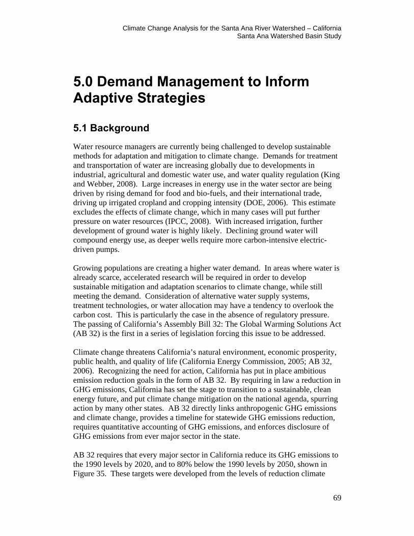
Climate Change Analysis for the Santa Ana River Watershed – California Santa Ana Watershed Basin Study
69
5.0 Demand Management to Inform Adaptive Strategies
5.1 Background
Water resource managers are currently being challenged to develop sustainable methods for adaptation and mitigation to climate change. Demands for treatment and transportation of water are increasing globally due to developments in industrial, agricultural and domestic water use, and water quality regulation (King and Webber, 2008). Large increases in energy use in the water sector are being driven by rising demand for food and bio-fuels, and their international trade, driving up irrigated cropland and cropping intensity (DOE, 2006). This estimate excludes the effects of climate change, which in many cases will put further pressure on water resources (IPCC, 2008). With increased irrigation, further development of ground water is highly likely. Declining ground water will compound energy use, as deeper wells require more carbon-intensive electric-driven pumps. Growing populations are creating a higher water demand. In areas where water is already scarce, accelerated research will be required in order to develop sustainable mitigation and adaptation scenarios to climate change, while still meeting the demand. Consideration of alternative water supply systems, treatment technologies, or water allocation may have a tendency to overlook the carbon cost. This is particularly the case in the absence of regulatory pressure. The passing of California’s Assembly Bill 32: The Global Warming Solutions Act (AB 32) is the first in a series of legislation forcing this issue to be addressed. Climate change threatens California’s natural environment, economic prosperity, public health, and quality of life (California Energy Commission, 2005; AB 32, 2006). Recognizing the need for action, California has put in place ambitious emission reduction goals in the form of AB 32. By requiring in law a reduction in GHG emissions, California has set the stage to transition to a sustainable, clean energy future, and put climate change mitigation on the national agenda, spurring action by many other states. AB 32 directly links anthropogenic GHG emissions and climate change, provides a timeline for statewide GHG emissions reduction, requires quantitative accounting of GHG emissions, and enforces disclosure of GHG emissions from ever major sector in the state. AB 32 requires that every major sector in California reduce its GHG emissions to the 1990 levels by 2020, and to 80% below the 1990 levels by 2050, shown in Figure 35. These targets were developed from the levels of reduction climate
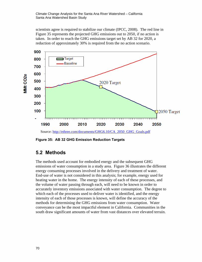
Climate Change Analysis for the Santa Ana River Watershed – California Santa Ana Watershed Basin Study
70
scientists agree is required to stabilize our climate (IPCC, 2008). The red line in Figure 35 represents the projected GHG emissions out to 2050, if no action is taken. In order to reach the GHG emissions target set by AB 32 for 2020, a reduction of approximately 30% is required from the no action scenario.
Figure 35: AB 32 GHG Emission Reduction Targets
5.2 Methods
The methods used account for embodied energy and the subsequent GHG emissions of water consumption in a study area. Figure 36 illustrates the different energy consuming processes involved in the delivery and treatment of water. End-use of water is not considered in this analysis; for example, energy used for heating water in the home. The energy intensity of each of these processes, and the volume of water passing through each, will need to be known in order to accurately inventory emissions associated with water consumption. The degree to which each of the processes used to deliver water is identified, and the energy intensity of each of those processes is known, will define the accuracy of the methods for determining the GHG emissions from water consumption. Water conveyance can be the most impactful element in California. Communities in the south draw significant amounts of water from vast distances over elevated terrain.
Source: http://ethree.com/documents/GHG6.10/CA_2050_GHG_Goals.pdf
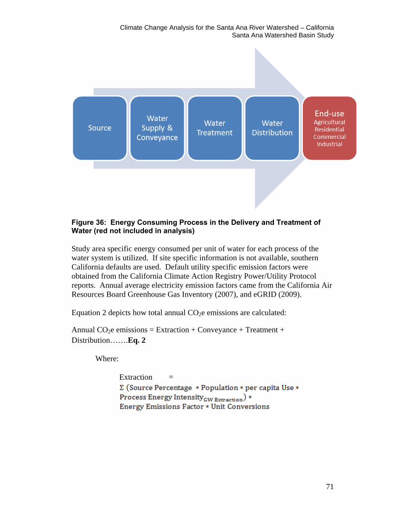
Climate Change Analysis for the Santa Ana River Watershed – California Santa Ana Watershed Basin Study
71
Figure 36: Energy Consuming Process in the Delivery and Treatment of Water (red not included in analysis) Study area specific energy consumed per unit of water for each process of the water system is utilized. If site specific information is not available, southern California defaults are used. Default utility specific emission factors were obtained from the California Climate Action Registry Power/Utility Protocol reports. Annual average electricity emission factors came from the California Air Resources Board Greenhouse Gas Inventory (2007), and eGRID (2009). Equation 2 depicts how total annual CO2e emissions are calculated:
Annual CO2e emissions = Extraction + Conveyance + Treatment + Distribution…….Eq. 2
Where:
Extraction =
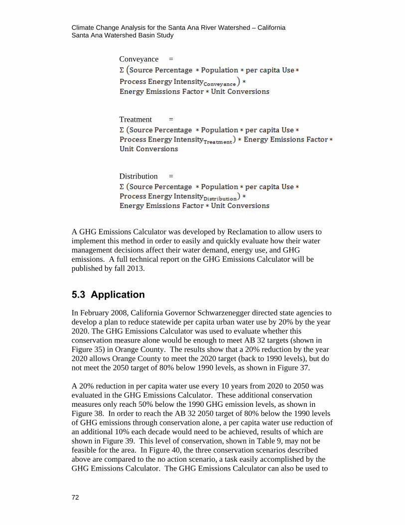
Climate Change Analysis for the Santa Ana River Watershed – California Santa Ana Watershed Basin Study
72
Conveyance =
Treatment =
Distribution =
A GHG Emissions Calculator was developed by Reclamation to allow users to implement this method in order to easily and quickly evaluate how their water management decisions affect their water demand, energy use, and GHG emissions. A full technical report on the GHG Emissions Calculator will be published by fall 2013.
5.3 Application
In February 2008, California Governor Schwarzenegger directed state agencies to develop a plan to reduce statewide per capita urban water use by 20% by the year 2020. The GHG Emissions Calculator was used to evaluate whether this conservation measure alone would be enough to meet AB 32 targets (shown in Figure 35) in Orange County. The results show that a 20% reduction by the year 2020 allows Orange County to meet the 2020 target (back to 1990 levels), but do not meet the 2050 target of 80% below 1990 levels, as shown in Figure 37. A 20% reduction in per capita water use every 10 years from 2020 to 2050 was evaluated in the GHG Emissions Calculator. These additional conservation measures only reach 50% below the 1990 GHG emission levels, as shown in Figure 38. In order to reach the AB 32 2050 target of 80% below the 1990 levels of GHG emissions through conservation alone, a per capita water use reduction of an additional 10% each decade would need to be achieved, results of which are shown in Figure 39. This level of conservation, shown in Table 9, may not be feasible for the area. In Figure 40, the three conservation scenarios described above are compared to the no action scenario, a task easily accomplished by the GHG Emissions Calculator. The GHG Emissions Calculator can also be used to
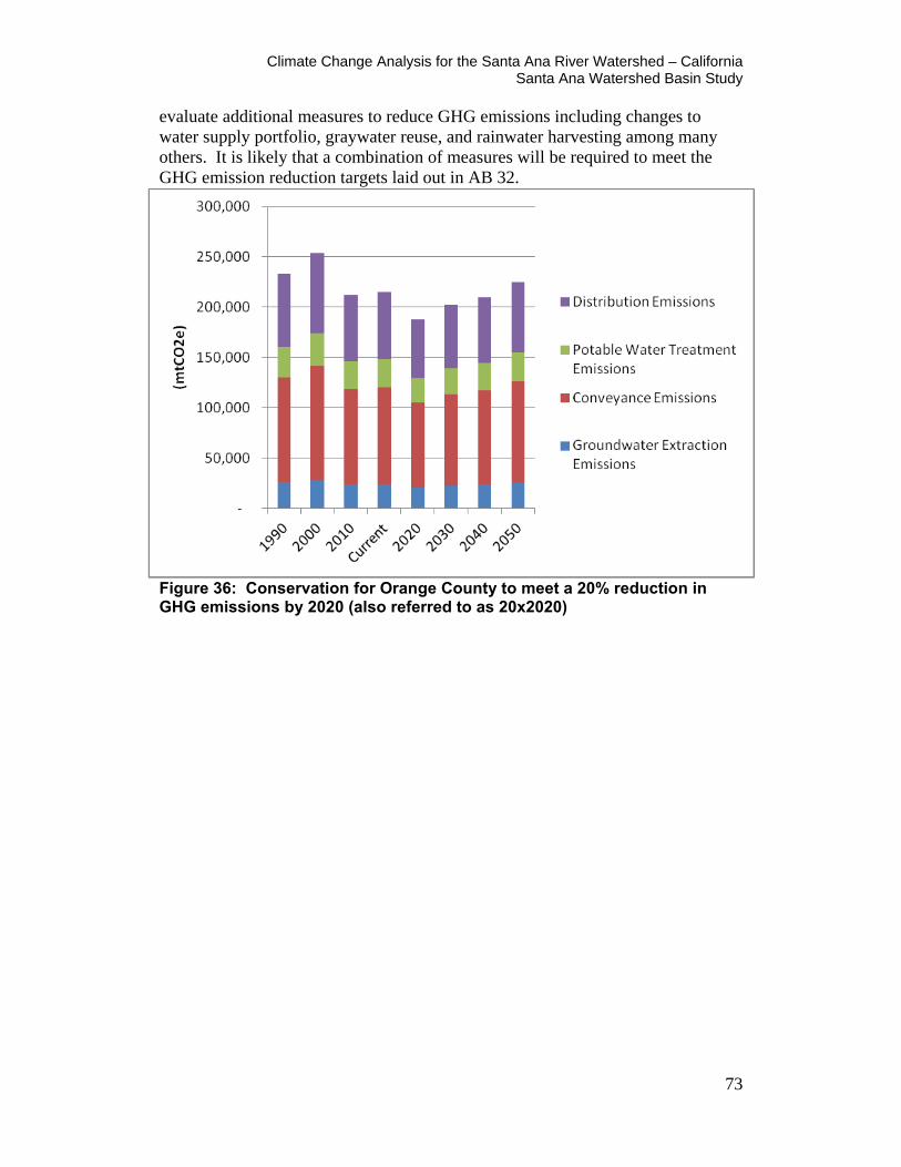
Climate Change Analysis for the Santa Ana River Watershed – California Santa Ana Watershed Basin Study
73
evaluate additional measures to reduce GHG emissions including changes to water supply portfolio, graywater reuse, and rainwater harvesting among many others. It is likely that a combination of measures will be required to meet the GHG emission reduction targets laid out in AB 32.
Figure 36: Conservation for Orange County to meet a 20% reduction in GHG emissions by 2020 (also referred to as 20x2020)
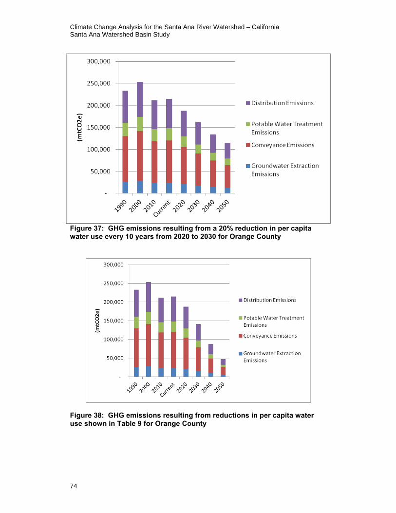
Climate Change Analysis for the Santa Ana River Watershed – California Santa Ana Watershed Basin Study
74
Figure 37: GHG emissions resulting from a 20% reduction in per capita water use every 10 years from 2020 to 2030 for Orange County
Figure 38: GHG emissions resulting from reductions in per capita water use shown in Table 9 for Orange County

Climate Change Analysis for the Santa Ana River Watershed – California Santa Ana Watershed Basin Study
75
Figure 39: Comparison of GHG emissions resulting from conservation scenarios
Table 9: Conservation measures required to meet AB 32 2050 target
6.0 Uncertainties This analysis was designed to take advantage of best available datasets and modeling tools and to follow methodologies documented in peer-reviewed literature. However, there are a number of analytical uncertainties that are not reflected in study results, including uncertainties associated with the following analytical areas that can be grouped under two categories: climate projection information and assessing hydrologic impacts that inform many of the Basin Study FAQs.
6.1 Climate Projection Information
6.1.1 Global Climate Forcing Although surface water hydrologic projections often consider future climate projections representing a range of future greenhouse emission paths, the uncertainties associated with these pathways are often not explored. Such uncertainties include those introduced by assumptions about technological and
1990 2000 2010 2020 2030 2040 2050Per Capita Water Use (gpd) 240 221 175 140 98 59 29Decadal Conservation Rate -8% -21% -20% -30% -40% -50%
Historical and Projected Per Capita Water Use
Climate Change Analysis for the Santa Ana River Watershed – California Santa Ana Watershed Basin Study
76
economic developments, globally and regionally; how those assumptions translate into global energy use involving GHG emissions; and biogeochemical analysis to determine the fate of GHG emissions in the oceans, land, and atmosphere. Also, not all the uncertainties associated with climate forgings are associated with GHG assumptions. Considerable uncertainty remains associated with natural forcings, with the cooling influence of aerosols being regarded as the most uncertain on a global scale (e.g., figure SPM-2 in IPCC 2007).
6.1.2 Global Climate Simulations While the activity presented in this report considers climate projections produced by state-of-the-art coupled ocean-atmosphere climate models, there are still uncertainties about the scientific understanding of physical processes that affect climate. For example, how to represent such processes in GCMs (e.g., atmospheric circulation, clouds, ocean circulation, deep ocean heat update, ice sheet dynamics, sea level, land cover effects from water cycle, vegetative, and other biological changes); and how to do so in a mathematically efficiently manner, given computational limitations. Still, these models have shown an ability to simulate the influence of increasing GHG emissions on global climate (IPCC 2007).
6.1.3 Climate Projection Bias Correction Surface water hydrologic projections inherit GCM biases toward being too wet, too dry, too warm, or too cool. Such systematic biases in GCMs should be identified and accounted for through bias-correction of climate projections, prior to use in impacts studies. Bias correction of climate projections data affects results on incremental runoff and water supply response.
6.1.4 Climate Projection Spatial Downscaling The Basin Study uses projections that have been spatially disaggregated on a monthly time step (following GCM bias correction on a monthly time step). Although this technique has been used to support numerous water resources impacts studies (e.g., Van Rheenan et al., 2004; Maurer, 2007; Anderson et al., 2008; Reclamation, 2008; Reclamation, 2010; Elsner et al., 2010), uncertainties remain about the limitations of empirical downscaling methodologies. One potential limitation relates to how empirical methodologies require historical reference information use on spatial climatic patterns at the downscaled spatial resolution. These finer-grid patterns are implicitly related to historical large-scale atmospheric circulation patterns, which presumably would change somewhat with global climate change. Application of the historical finer-grid spatial patterns to guide downscaling of future climate projections implies an assumption that the historical relationship between finer-grid surface climate patterns and large-scale atmospheric circulation is still valid under the future climate. In other words, the relationship is assumed to have statistical stationarity, meaning the joint probability distribution does not change when shifted in time or space. In actuality, it is possible that such stationarity will not hold at various space and time scales, over various locations, and for various climate variables. However,

Climate Change Analysis for the Santa Ana River Watershed – California Santa Ana Watershed Basin Study
77
the significance of potential non-stationarity in empirical downscaling methods, and the need to utilize alternative downscaling methodologies remains not well understood.
6.2 Assessing Hydrologic Impacts
6.2.1 Generating Weather Sequences Consistent with Climate Projections The temporal disaggregation method developed first by Wood et al., (2002), was used in this Basin Study to translate monthly BCSD climate projections into daily VIC weather forcings. However, other techniques might have been considered. Choice of weather generation technique depends on aspects of climate change that are being targeted in a given study. Preference among available techniques remains to be established. Various characteristics, such as that the resampling approach, does not allow daily temperature ranges to vary from those selected with the sample, make the disaggregation approach unsuitable for studies focusing on potential changes in the diurnal range of temperature. In contrast, it may be sufficient for monthly time step hydrological assessments if the disaggregation is performed with thoughtful sampling constraints.
6.2.2 Natural Runoff Response This Basin Study analyzes natural runoff response to changes in precipitation, temperature, and change in natural vegetation PET while holding other watershed features constant. Other watershed features might be expected to change as climate changes and affects runoff (e.g., vegetation affecting evapotranspiration and infiltration, etc.). On the matter of land cover response to climate change, the runoff models’ calibrations would have to change if land cover changed, because the models were calibrated to represent the historical relationship between weather and runoff as mediated by historical land cover. Adjustment to watershed land cover and model parameterizations are difficult to consider due to lack of available information to guide such an adjustment. Eco-hydrological frameworks, perhaps involving dynamic vegetation response, may be suitable to represent such land surface changes for studies in which such sensitivities are important.
6.2.3 Hydrologic Modeling The hydrology model used in the Basin Study excludes ground water interaction with surface water systems. The fate of precipitation is modeled as loss only to runoff and evapotranspiration; and loss of precipitation to deep percolation and return flows to stream channel networks are not considered in the VIC hydrology model. The groundwater impacts in the basin are simulated using a simplified tool.
6.2.4 Bias and Calibration Where the VIC applications have been calibrated, they can reproduce historical natural streamflow with little bias. Where the VIC applications have not been

Climate Change Analysis for the Santa Ana River Watershed – California Santa Ana Watershed Basin Study
78
calibrated, they can exhibit significant bias. The location-specific implications of calibration, or lack thereof, on the conclusions of the study have not been quantified.
6.2.5 Time Resolution of the Applications Simulations were conducted at daily time steps, while the applications were calibrated to reproduce monthly and annual runoff characteristics at a subset of locations in the basin. For this reason, users should cautiously interpret the daily hydrologic information coming from these simulations. The daily runoff information is physically consistent with assumed weather forcings and hydrologic model structure; however, there could be significant simulation biases at the submonthly level.

Climate Change Analysis for the Santa Ana River Watershed – California Santa Ana Watershed Basin Study
79
Page Intentionally Left Blank
7.0 References Anderson, J., F. Chung, M. Anderson, L. Brekke, D. Easton, M. Ejeta, R.
Peterson, and R. Snyder. 2008. “Progress on Incorporating Climate Change into Management of California’s Water Resources.” Climatic Change, Springer, Netherlands, Volume 89, Supplement 1, pp. 91–108. Published online December 22, 2007. ISSN: 0165-0009 (Print) 1573–1480 (Online) DOI: 10.1007/s10584-007-9353-1.
Anning, David W., 2011. "Modeled Sources, Transport, and Accumulation of Dissolved Solids in Water Resources of the Southwestern United States." Journal of the American Water Resources Association (JAWRA) 1-23. DOI: 10.1111/j.1752-1688.2011.00579.x
Baldocchi, D., and S. Wong. 2006. An Assessment of the Impacts of Future CO2 and Climate on California Agriculture. Prepared for California Energy Commission Public Interest Energy Research Program, Project Report CEC-500-2005-187-SF.
Barnett, T.P., D.W. Pierce, H.G. Hidalgo, C. Bonfils, B.D. Santer, T. Das, G. Bala, A. Wood, T. Nazawa, A. Mirin, D. Cayan, and M. Dettinger. 2008. “Human-induced changes in the hydrology of the Western United States.” Science, 319(5866), 1080–1083, doi:10.1126/science.1152538.
Bonfils, C., P.B. Duffy, B.D. Santer, T.M.L. Wigley, D.B. Lobell, T.J. Phillips, and C. Doutriaux. 2007. “Identification of External Influences on Temperatures in California,” Prepared for California Energy Commission Public Interest Energy Research Program, Project Report CEC-500-2007-047.
Bonfils, C., D.W. Pierce, B.D. Santer, H. Hidalgo, G. Bala, T. Das, T. Barnett, C. Doutriaux, A.W. Wood, A, Mirin, and T. Nazawa. 2008. “Detection and attribution of temperature changes in the mountainous Western United States.” Journal of Climate 21(23): 6404–6424, doi:10.1175/ 2008JCLI2397.1.
Brekke, L.D., E.P. Maurer, J.D. Anderson, M.D. Dettinger, E.S. Townsley, A. Harrison, and T. Pruitt. 2009b. “Assessing Reservoir Operations Risk under Climate Change.” Water Resour. Res., doi:10.1029/ 2008WR006941
Bromirski, Miller, Flick, Auad, "Dynamical Suppression of Coastal Sea Level Rise." JGRC, sub. Oct. 2010, rev. 1 Jan. 2011, rev. 2 Mar. 2011.
Climate Change Analysis for the Santa Ana River Watershed – California Santa Ana Watershed Basin Study
80
Burkett, V., and J. Kusler. 2000. Climate Change: “Potential Impacts and Interactions in Wetlands of the United States.” Journal of the American Water Resources Association. Vol. 36, No. 2, p.313–320, 10.1111/j.1752-1688.2000.tb04270.x.
California Department of Water Resources (2009). “California State Water Project Overview.” California Department of Water Resources, <http://www.water.ca.gov/swp/>, (October 21, 2009).
California Energy Commission (2003). “ California Agricultural Water Electrical Energy Requirements.” California Energy Commission, Sacramento, Ca.
California Energy Commission (2005). “California’s Water-Energy Relationship.” California Energy Commission, Sacramento, Ca.
California Energy Commission (2006). “Refining Estimates of Water-Related Energy in California.” California Energy Commission, Sacramento, Ca.
California Department of Forestry and Fire Protection, Fire and Resource Assessment Program. 2010. California’s Forests and Rangelands: 2010 Assessment. Chapter 3.7. http://frap.fire.ca.gov/assessment2010.html.
Cayan, D.R., S.A. Kammerdiener, M.D. Dettinger, J.M. Caprio, and D.H. Peterson. 2001. “Changes in the Onset of Spring in the Western United States.” Bulletin of the American Meteorology Society 82(3): 399–415.
Cayan D, M Tyree, M Dettinger, H Hidalgo, T Das, E Maurer, P Bromirski, N Graham, R Flick (2009). Climate Change Scenarios and Sea Level Rise Estimates for the California 2008 Climate Change Scenarios Assessment. California Climate Change Center, California Energy Commission Paper No. CEC-500-2009-014-D.
CCSP (Climate Change Science Program). 2009. Thresholds of Climate Change in Ecosystems. A report by the U.S. Climate Change Science Program and the subcommittee on Global Change Research. Fagre, D.B., C.W.
Christensen, N.S. and D.P. Lettenmaier. 2007. “A multimodel ensemble approach to assessment of climate change impacts on the hydrology and water resources of the Colorado River basin,” Hydrology and Earth System Sciences, 11, 1417-1434.
Christensen, N.S., A.W. Wood, D.P. Lettenmaier, and R.N. Palmer. 2004. “Effects of climate change on the hydrology and water resources of the Colorado river basin,” Climate Change, 62(1-3), 337-363
City of Santa Ana. 2006. “Santa Ana River Vision Plan: History of the Santa Ana River,” Adopted June 13, 2006.
Climate Change Analysis for the Santa Ana River Watershed – California Santa Ana Watershed Basin Study
81
Crookston, N. L. 2009. “Species-Climate Profile for Jeffrey Pine.” Tree Species Climate Profiles. Moscow Forestry Sciences Laboratory. http://forest.moscowfsl.wsu.edu/climate/species/index.php.
Crookston, N. L. G.E. Rehfeldt, G.E. Dixon, A.R. Weiskittel. 2010. “Addressing Climate Change in the Forest Vegetation Simulator to Assess Impacts on Landscape Forest Dynamics.” Forest Ecology and Management. Moscow Forestry Sciences Laboratory http://www.fs.fed.us/rm/pubs_other/rmrs_2010_crookston_n001.pdf
Dai,"A."(2011)."Drought"under"global"warming:"a"review."Wiley"Interdisciplinary"Reviews:"Climate"Change,"2: 45–65." doi: 10.1002/wcc.81
Das, T., H.G. Hidalgo, M.D. Dettinger, D.R. Cayan, D.W. Pierce, C. Bonfils, T.P. Barnett, G. Bala, and A. Mirin. 2009. “Structure and Detectability of Trends in Hydrological Measures over the Western United States.” Journal of Hydrometeorology, Vol. 10, doi:10.1175/2009JHM1095.1.
Dettinger, M.D., and D.R. Cayan. 1995. “Large-scale Atmospheric Forcing of Recent Trends toward Early Snowmelt Runoff in California.” Journal of Climate, Vol. 8(3).
DOE (2006). “Energy Demands on Water Resources: Report to Congress on the Interdependency of Energy and Water.” United States Department of Energy.
Federal Emergency Management Agency (FEMA). 2007. “Guidelines and specifications for flood hazard mapping partners: Atlantic Ocean and Gulf of Mexico coastal guidelines update,” FEMA Region VI, FEMA Headquarters.
Ficke, A.D., C.A. Myrick, and L.J.Hansen. 2007. “Potential impacts of global climate change fisheries.” Reviews in Fish Biology and Fisheries, 17(4): 581–613, 10.1007/s11160-007-9059-5.
Gershunov, A., D.R. Cayan, and S.F. Iacobellis. 2009. “The Great 2006 heat wave over California and Nevada: Signal of an Increasing Trend.” J. Climate., 22(23), 6181–6203.
Gershunov, A., and K. Guirguis (2012), California heat waves in the present and future, Geophys. Res. Lett.,39, L18710, doi:10.1029/2012GL052979.
Griffis, V. W. and Stedinger, J. R. 2007. “Incorporating Climate Change and Variability into Bulletin 17B LP3 Model,” World Environmental and Water Resources Congress 2007: Restoring Our Natural Habitat, American Society of Civil Engineers, 8 pp.

Climate Change Analysis for the Santa Ana River Watershed – California Santa Ana Watershed Basin Study
82
Haak, A.L., J.E. Williams, D. Isaak, A. Todd, C. C. Muhlfeld, J.L. Kershner, R. Gresswell, S. Hostetler, and H. Neville. 2010In review. “The potential influence of changing climate on the persistence of western trout and grayling.” USGS Open File Report, Reston, Virginia, USA.
Hall, Alex; Sun, Fengpeng; Walton, Daniel; Capps, Scott; Qu, Xin; Huang, Hsin-Yuan; et al.(2012). Mid-Century Warming in the Los Angeles Region - Part I of the “Climate Change in the Los Angeles Region” projec. UC Los Angeles: Institute of the Environment and Sustainability. http://www.escholarship.org/uc/item/6v88k76b
Hamlet, A.F., and D.P. Lettenmaier. 2007. “Effects of 20th century warming and climate variability on flood risk in the Western United States.” Water Resources Research 43, W06427, doi:10.1029/2006WR005099.
Harou, J.J., J. Medellín-Azuara, T. Zhu, S.K. Tanaka, J.R. Lund, S. Stine, M.A. Olivares, and M.W. Jenkins. 2010. “Economic consequences of optimized water management for a prolonged, severe drought in California.” Journal of Water Resources Research, Vol. 46, W05522, doi:10.1029/2008WR007681.
Hayhoe, K. et al., 2004. Emissions pathways, climate change, and impacts on California. PNAS, 101:34, pp 12422-12427.
Hidalgo,H., D. Cayan, and M. Dettinger. 2005. “Sources of Variability of Evapotranspiration in California.” Journal of Hydrometeorology 6: 3–19.
Hidalgo H.G., T. Das, M.D. Dettinger, D.R. Cayan, D.W. Pierce, T.P. Barnett, G. Bala, A. Mirin, A.W. Wood, and C. Bonfils. 2009. “Detection and Attribution of Streamflow Timing Changes to Climate Change in the Western United States.” Journal of Climate 22(13): 3838, doi:10.1175/ 2008JCLI2470.1.
Hiltner, N. 2010. “Santa Ana River was wests greatest flood hazard,” The press Enterprise, August 21, 2010.
Hoerling, M., and J. Eischeid. 2007. “Past Peak Water in the Southwest.” Southwest Hydrology, 6(1):18–19: 35.
Hoerling M., J. Eischeid, and J. Perlwitz. 2010. “Regional Precipitation Trends: Distinguishing Natural Variability from Anthropogenic Forcing.” Journal of Climate (in press).
Hosking, J.R.M. and J.R. and Wallis. 1997. “Regional Frequency Analysis: An Approach Based on L-moments,” Cambridge University Press. ISBN 0-521-43045-3.

Climate Change Analysis for the Santa Ana River Watershed – California Santa Ana Watershed Basin Study
83
Interagency Committee on Water Data (IACWD). (1982). “Guidelines for determining flood flow frequency.” Bulletin No. 17B (revised and corrected), Hydrology Subcommittee, Washington, D.C. Read More: http://ascelibrary.org/doi/ref/10.1061/%28ASCE%291084-0699%282007%2912%3A3%28283%29
[IPCC] Intergovernmental Panel on Climate Change, 2006 IPCC Guidelines for National Greenhouse Gas Inventories, Prepared by the National Greenhouse Gas Inventories Programme, Eggleston H.S., Buendia
[IPCC] Intergovernmental Panel on Climate Change, The Physical Science Basis, Fourth Assessment, Working Group I Report (2007).
[ICLEI] ICLEI-Local Governments for Sustainability, Draft International Local Government GHG Emissions Analysis Protocol (April 21, 2008).
L., Miwa K., Ngara T. and Tanabe K. (eds) (2006). Katz, R. and Naveau, P. 2002. “Statistics of extremes in hydrology,” Advances in water Resources, 25, 1287-1304.
King C W and Webber M E 2008 Water intensity of transportation Environ. Sci. Technol. 42 7866-72
Knowles, N., M. Dettinger, and D. Cayan. 2007. Trends in Snowfall Versus Rainfall for the Western United States, 1949–2001. Prepared for California Energy Commission Public Interest Energy Research Program, Project Report CEC-500-2007-032.
Knowles, N. 2010. “Potential Inundation Due to Rising Sea Levels in the San Francisco Bay Region.” California Climate Change Center. San Francisco Estuary and Watershed Science, 8(1).
Kunkel, K.E., D.R. Easterling, K. Redmond, and K. Hubbard. 2003. “Temporal variations of estreme precipitation events in the United States: 1895–2000.” Geophysical Research Letters, Vol. 30, No. 17, 1900, doi:10.1029/2003GLO18052, 2003.
Lenihan, J. M., D. Bahelet, D. P. Nielson, R. Drapek. 2008. Response of vegetation distribution, ecosystem productivity, and fire to climate change scenarios for California. Climate Change, 87 (supply 1), pp. S215-S230. Doi 10.1007/s10584-007-9362-0.
Liang, X., D.P. Lettenmaier, E.F. Wood, and S.J. Burges. 1994. “A simple hydrologically based model of land surface water and energy fluxes for general circulation models,” Journal of Geophysical Research, 99(D7), 14415-14428.
Climate Change Analysis for the Santa Ana River Watershed – California Santa Ana Watershed Basin Study
84
Liang, X., E.F. Wood, and D.P. Lettenmaier. 1996. “Surface soil moisture parameterization of the VIC-2L model: Evaluation and modifications,” Glob Planet Change, 13” 195-206.
Lohmann, D., E. Raschke, B. Nijssen, and D.P. Lettenmaier, 1998: Regional scale hydrology: I. Formulation of the VIC-2L model coupled to a routing model. Hydrol. Sci. J., 43, 131-141.
Lundquist, J.D., M.D. Dettinger, I.T. Stewart, and D.R. Cayan. 2009. “Variability and Trends in Spring Runoff in the Western United States.” Climate warming in western North America—Evidence and environmental effects, University of Utah Press. pp. 63-76.
Madsen, T., and E. Figdor. 2007. “When It Rains It Pours - Global Warming and the Rising Frequency of Extreme Precipitation in the United States.” Environment America Research and Policy Center. Available online at http://www.environmentamerica.org/uploads/oy/ws/oywshWAwZy-EXPsabQKd4A/When-It-Rains-It-Pours----US---WEB.pdf.
Maurer, E.P., L. Brekke, T. Pruitt, and P.B. Duffy. 2007. “Fine-resolution climate projections enhance regional climate change impact studies,” Eos Trans. AGU, 88(47), 504.
Maurer, E.P., L.D. Brekke, and T. Pruitt. 2010. “Contrasting lumped and distributed hydrology models for estimating climate change impacts on California watersheds,” Journal of the American Water Resources Association (JAWRA) 46(5):1024–1035. DOI: 10.1111/j.1752-1688.2010.00473.x.
Elsner, M., L. Cuo, N. Voisin, J.S. Deems, A.F. Hamlet, J.A. Vano, K.E.B. Mickelson, S.Y. Lee, and D.P. Lettenmaier. 2010. “Implications of 21st century climate change for the hydrology of Washington State,” Climatic Change, DOI:10.1007/s10584-010-9855-0.
Moore, L. M. 2006. Jeffrey Pine Plant Guide. United States Department of Agriculture (USDA) Natural Resources Conservation Service (NRCS)
Moser, S., G. Franco, S. Pittiglio, W. Chou, and D. Cayan. 2009. The Future Is Now: An Update on Climate Change Science Impacts and Response Options for California. California Energy Commission, PIER Energy-Related Environmental Research Program, CEC-500-2008-071.
Mote, P.W., A.F. Hamlet, and E.P. Salathé. 2008. “Has spring snowpack declined in the Washington Cascades?” Hydrology and Earth System Sciences 12: 193–206.
Climate Change Analysis for the Santa Ana River Watershed – California Santa Ana Watershed Basin Study
85
Nijssen, B., D.P. Lettenmaier, X. Liang, S.W. Wetzel, and E.F. Wood. 1997. “Streamflow simulation for continental-scale river basins,” Water Resour. Res., 33, 711-724.
Null, S.E., J.H. Viers, and J.F. Mount. 2010. “Hydrologic Response and Watershed Sensitivity to Climate Warming in California’s Sierra Nevada.” PLoS One. Vol. 5(4): e9932, doi:10.1371/journalpone.0009932.
Payne, J.T., A.W. Wood, A.F. Hamlet, R.N. Palmer, and D.P. Lettenmaier. 2004. “Mitigating the effects of climate change on the water resources of the Columbia River basin,” Climate Change, 62(1-3):233-256.
Peterson, D.H., I. Stewart, and F. Murphy. 2008. “Principal Hydrologic Responses to Climatic and Geologic Variability in the Sierra Nevada, California.” San Francisco Estuary and Watershed Science 6(1): Article 3.
Pierce, D.W., T. Barnett, H. Hidalgo, T. Das, C. Bonfils, B.D. Santer, G. Bala, M. Dettinger, D. Cayan, A. Mirin, A.W. Wood, and T. Nazawa. 2008. “Attribution of declining Western U.S. snowpack to human effects.” Journal of Climate 21(23): 6425–6444, doi:10.1175/2008JCLI2405.1.
Pierce D., Das T., Cayan D., Maurer., Miller M., Bao Y., Kanamitsu M., Yoshimura K., Snder M., Sloan M., Franco G., Tyree M. 2011. "Probabilistic estimates of California climate change by the 2060s using statistical and dynamical downscaling." California Energy Commission, Contract Number: 500-07-042.
Rahmstorf, S. 2007. “A Semi-Empirical Approach to Projecting Future Sea-Level Rise.” Science, 315: 368–370.
Rauscher, S.A., J.S. Pal, N.S. Diffenbaugh, and M.M. Benedetti. 2008. “Future Changes in Snowmelt-driven Runoff Timing Over the Western United States.” Geophysical Research Letters, Vol. 35, L16703, doi:10.1029/ 2008GL034424.
Reclamation. 2008. “Sensitivity of Future CVP/SWP Operations to Potential Climate Change and Associated Sea Level Rise,” Appendix R in Biological Assessment on the Continued Long-term Operations of the Central Valley Project and the State Water Project. Prepared by the U.S. Department of the Interior, Bureau of Reclamation, Mid-Pacific Region, Central Valley Operations Office, Sacramento, California. August 2008. 134 pp.
Reclamation. 2010. Climate Change and Hydrology Scenarios for Oklahoma Yield Studies, prepared by the U.S. Department of the Interior, Bureau of Reclamation, Technical Services Center, Denver Colorado. April 2010. 71 pp.
Climate Change Analysis for the Santa Ana River Watershed – California Santa Ana Watershed Basin Study
86
Reclamation. 2011. West-wide climate risk assessments: Bias-corrected and spatially downscaled surface water projections, Tech. Memo., 86-68210-2011-01, 138 pp., Tech. Serv. Cent., U.S. Dep. of the Inter., Denver Colo., March.
Regonda, S.K., B. Rajagopalan, M. Clark, and J. Pitlick. 2005. “Seasonal Cycle Shifts in Hydroclimatology Over the Western United States.” Journal of Climate 18(2): 372–384.
Santa Ana River Mainstem Project (SARP). Web. 2013. “SARP History,” ocflood.com.
Seager R., M.Ting, I. Held, Y. Kushnir, J. Lu, and G. Vecchi. 2007. “Model Projections of an Imminent Transition to a More Arid Climate in Southwestern North America.” Science 316(5828): 1181–1184.
Shin, S., and P.D. Sardeshmukh. 2010. “Critical influence of the pattern of Tropical ocean warming on remote climate trends.” Climate Dynamics, DOI 10.1007/s00382-009-0732-3.
Sun, Y., S.Solomon, A.Dai, and R.W. Portmann. 2007. “How Often Will It Rain?” J. Climate, 20, 4801–4818, doi: 10.1175/JCLI4263.1.
Taylor, K.E., R.J. Stouffer, and G.A. Meehl, 2011. A Summary of the CMIP5 Experiment Design. January 22, 2011, 33 p., available at: http://cmip-pcmdi.llnl.gov/cmip5/docs/Taylor_CMIP5_design.pdf.
U.S. Interagency Advisory Committee on Water Data. 1982. “Guidelines for determining flood flow frequency, Bulletin 17-B of the Hydrology Subcommittee.” Reston, Virginia, U.S. Geological Survey, Office of Water Data Coordination.
Van Rheenen, N.T., A.W. Wood, R.N. Palmer, D.P. Lettenmaier. 2004. “Potential implications of PCM climate change scenarios for Sacramento-San Joaquin River Basin hydrology and water resources,” Climatic Change, 62, 257-281
Vermeera, M., and S. Rahmstorf. 2009. “Global sea level linked to global temperature.” Proceedings of the National Academy of Sciences. Available online at www.pnas.org/cgi/doi/10.1073/pnas.0907765106.
Vicuna, S., and J.A. Dracup. 2007. “The Evolution of Climate Change Impact Studies on Hydrology and Water Resources in California.” Climatic Change 82(3–4): 327–350.
Climate Change Analysis for the Santa Ana River Watershed – California Santa Ana Watershed Basin Study
87
Vicuna, S., E.P. Maurer, B. Joyce, J.A. Dracup, and D. Purkey, 2007. “The Sensitivity of California Water Resources to Climate Change Scenarios,” Journal of the American Water Resources Association 43:482-498.
Vicuna, S., J.A. Dracup, J.R. Lund, L.L. Dale, and E.P. Maurer. 2010. “Basin-scale water system operations with uncertain future climate conditions: Methodology and case studies.” Journal of Water Resources Research, Vol. 46, W04505, doi:10.1029/2009WR007838, 2010.
Villarini, G., F. Serinaldi, J.A. Smith, and W.F. Krajewski. 2009. “On the stationarity of annual flood peaks in the continental United States during the 20th century.” Water Resources Research, Vol. 45, W08417, doi:10.1029/2008WR007645.
Wood, A.W. , E.P. Maurer, A. Kumar, and D.P. Lettenmaier. 2002. “Long-range experimental hydrologic forecasting for the Eastern United States,” J. Geophysical Research-Atmospheres, 107(D20), 4429, doi:10.1029/2001JD000659.
Wood, A.W., L.R. Leung, V. Sridhar, and D.P. Lettenmaier. 2004. “Hydrologic implications of dynamical and statistical approaches to downscaling climate model outputs,” Climate Change, 15, 189-216.