CLIMATE CHANGE, AGRICULTURE AND TRADE POLICY:

CGE ANALYSES AT REGIONAL, NATIONAL AND GLOBAL LEVEL

A THESIS SUBMITTED TO

THE GRADUATE SCHOOL OF SOCIAL SCIENCES

OF

MIDDLE EAST TECHNICAL UNIVERSITY

BY

HASAN DUDU

IN PARTIAL FULFILLMENT OF THE REQUIREMENTS

FOR

THE DEGREE OF DOCTOR OF PHILOSOPHY

IN

THE DEPARTMENT OF ECONOMICS

DECEMBER, 2013

Approval of the Graduate School of Social Sciences

Prof. Dr. Meliha Altunışık

Director

I certify that this thesis satisfies all the requirements as a thesis for the degree of

Doctor of Philosophy.

Prof. Dr. Nadir Öcal

Head of Department

This is to certify that we have read this thesis and that in our opinion it is fully

adequate, in scope and quality, as a thesis for the degree of Doctor of Philosophy.

Prof. Dr. Nadir Öcal

Supervisor

Examining Committee Members (first name belongs to the chairperson of the jury

and the second name belongs to supervisor)

Prof. Dr. Halis Akder (METU, ECON)

Prof. Dr. Nadir Öcal (METU, ECON)

Prof. Dr. Erol Çakmak (TED Uni., ECON)

Assoc. Prof. Dr. Ebru Voyvoda (METU, ECON)

Assoc. Prof. Dr. Ozan Eruygur (Gazi Uni, ECON)

iii

PLAGIARISM

I hereby declare that all information in this document has been obtained and

presented in accordance with academic rules and ethical conduct. I also

declare that, as required by these rules and conduct, I have fully cited and

referenced all material and results that are not original to this work.

Name, Last name : Hasan Dudu

Signature :

iv

ABSTRACT

CLIMATE CHANGE, AGRICULTURE AND TRADE POLICY:

CGE ANALYSES AT REGIONAL, NATIONAL AND GLOBAL LEVEL

Dudu, Hasan

Ph.D., Department of Economics

Supervisor: Prof. Dr. Nadir Öcal

December 2013, 228 pages

This thesis investigates the effects of climate change on the Turkish economy by

using computable general equilibrium (CGE) models at regional, national and

global level. The physical impact of climate change is first translated into yield and

irrigation requirement shocks by using a crop-hydrology model developed for this

study. Then these are introduced into the CGE models as productivity shocks to

investigate their effects on the overall economy. Simulation results suggest that

climate change will come into play after 2035, and its effects on the economy will

get worse after 2060. The final economic effects at regional and global levels will

depend on the location and structure of agricultural production.

Trade liberalization is considered as a policy response to contain the negative

impact of the climate change. The results indicate that trade liberalization helps, but

the positive effects are limited. International trade plays a key role in the response

of the economy to the climate change shocks. Trade liberalization with the

European Union is found to have positive effects on welfare of households,

however these effects are low compared to the harm caused by climate change.

Moreover, it was also noted that these positive effects increased as climate change

effects are worsened.

v

At the global level, the simulation results suggest that there is a significant

uncertainty about the impact of climate change on the global economy. The effects

are not homogenous for different regions of the world or different sectors in a

region. On the other hand, effects of trade liberalization are not affected by the

uncertainty in the climate change scenarios. Our results suggest that adverse effects

of climate change on welfare can be alleviated by trade liberalization in most parts

of the world.

Keywords: Climate Change, International Trade, Turkey, Agriculture, Computable

General Equilibrium

vi

ÖZ

İKLİM DEĞİŞİKLİĞİ, TARIM VE TİCARET POLİTİKASI:

BÖLGESEL, ULUSAL VE KÜRESEL DÜZEYDE BİR HGD ANALİZİ

Dudu, Hasan

Doktora, İktisat Bölümü

Tez Yöneticis: Prof. Dr. Nadir Öcal

Aralık 2013, 228 sayfa

Bu tez iklim değişikliğinin Türkiye ekonomisi üzerindeki etkilerini bölgesel, ulusal

ve küresel düzeyde hesaplanabilir genel denge (HGD) modelleri ile incelemektedir.

Öncelikle iklim değişikliğinin fiziksel etkileri bu çalışma için geliştirilmiş olan bir

bitki-sulama modeli ile verim ve sulama gereksinimi değişimlerine

dönüştürülmüştür. Daha sonar bu değişimler HGD modeline üretkenlik şokları

olarak kullanılmıştır.

Sonuçlar iklim değişikliğinin 2035 yılından itibaren etkili olmaya başlayacağını,

2060 yılından sonra etkilerin ağırlaşacağını göstermektedir. Hem bölgesel hem de

küresel etkiler konuma ve tarımsal üretimin yapısına göre değişikliklik

göstermektedir. Uluslararası ticaret ekonominin iklim değişikliği şoklarına verdiği

tepkide anahtar rol oynamaktadır. Ulusal düzeyde ticaret serbesleştirmesinin etkileri

de incelenmiştir. Avrupa Birliği ile yapılacak olan bir ticaret serbestleşmesi refahı

arttırmakta ancak bu artış iklim değişikliğinin sebep olduğu zararı karşılamak

konusunda düşük kalmaktadır. Ancak refah artışı iklim değişikliğinin etkileri

ağırlaştıkça artmaktadır.

Benzetim sonuçları küresel düzeyde iklim değişikliğinin etkilelerinin olası

etkilerinin geniş bir yelpazeye yayıldığını göstermektedir. Sonuçlar dünyanın farklı

vii

bölgeleri ve bir bölgedeki farklı sektörler için değişiklikler göstermektedir. Diğer

taraftan, ticaret serbestleşmesinin etkileri genellikle varsayılan iklim değişikliği

senaryosundan bağımsızdır. Sonuçlar, iklim değişikliğinin olumsuz etkilerinin

küresel çaptaki yapılacak bir ticaret serbestleşmesi ile hafifletilebileceğini

göstermektedir.

Anahtar Kelimeler: İklim değişikliği, Uluslararası Ticaret, Tarım, Türkiye,

Hesaplanabilir Genel Denge

viii

In memory of my grandmother, Feride Dudu

ix

ACKNOWLEDGMENTS

This thesis would not have existed without the guidance and support of Dr. Erol

Çakmak. I am deeply indebted for his encouraging and understanding attitude

towards me and my work which made the process enjoyable and allowed me to

push my frontiers as much as possible. He was also a generous mentor about life

and helped me to adopt a sense of perfection and hard-work.

I am also indebted to Dr. Nadir Öcal not only for accepting this work for

supervision at a late stage, but also for his support throughout my Ph.D. studies. I

wish to express my sincere gratitude to Dr. Halis Akder and Dr. Ebru Voyvoda for

their constructive and invaluable recommendations.

I would also like to thank to Dr. Ozan Eruygur, who treated me like a brother from

the very beginning of my academic career. His inspiring vision and unique

approach have always showed me the right path whenever I felt lost during my

studies.

I am thankful to Dr. Kemal Sarıca, Dr. Wally Tyner, Dr. Xinshen Diao, and Dr.

James Thurlow for their insightful comments during the course of my studies. I am

also thankful to Annette Morcos for her support in the final editing of the text.

Some parts of this work is supported by the CAPRI-RD project financed by

European Commission within the 7th

Framework Programmé and “Economic

Growth in the Euro-Med Area through Trade Integration Project” financed by JRC-

IPTS.

I should also mention my gratitude to my family for their precious support. They

have always been there for me whenever I needed someone to rely on. The last but

not the least, I would also like to thank to my colleagues in the Department of

Economics of METU, especially to Ünal Töngür.

x

TABLE OF CONTENTS

PLAGIARISM............................................................................................................. iii

ABSTRACT ................................................................................................................ iv

ÖZ .............................................................................................................................. vi

ACKNOWLEDGMENTS ........................................................................................... ix

TABLE OF CfigfigureONTENTS ............................................................................... x

LIST OF FIGURES .................................................................................................... xii

LIST OF TABLES ................................................................................................... xvii

LIST OF ABBREVIATIONS ................................................................................. xviii

CHAPTER

1. INTRODUCTION ................................................................................................. 1

2. AN INTEGRATED ANALYSIS OF ECONOMY-WIDE EFFECTS OF

CLIMATE CHANGE FOR TURKEY ................................................................. 5

2.1 Climate Change ................................................................................................ 6

2.2 Integrated Modeling Approach ...................................................................... 10

2.2.1 Crop Water Requirement Model ............................................................ 14

2.2.2 Regional CGE model.............................................................................. 20

2.3 Description of Data and Simulations.............................................................. 24

2.4 Results and Discussion ................................................................................... 30

2.5 Conclusion ...................................................................................................... 38

3. CLIMATE CHANGE, AGRICULTURE AND TRADE

LIBERALIZATION: A DYNAMIC CGE ANALYSIS FOR TURKEY ........... 40

3.1 Description of the model ................................................................................ 41

3.2 Description of Data ........................................................................................ 47

3.3 Trade Liberalization between EU and Turkey ............................................... 52

3.3.1 Scenario Design ...................................................................................... 55

3.3.2 Simulation Results .................................................................................. 65

3.4 Conclusion ...................................................................................................... 92

4. TRADE POLICY AS A GLOBAL ADAPTATION MEASURE TO

CLIMATE CHANGE ......................................................................................... 95

xi

4.1 Modelling framework: GTAP Model ............................................................. 98

4.2 Scenario Design ........................................................................................... 100

4.3 Results and discussions ................................................................................ 104

4.3.1 Effects of Climate Change ................................................................... 104

4.3.2 Effects of Trade Liberalization ............................................................ 109

4.4 Conclusion.................................................................................................... 123

5. CONCLUDING REMARKS ............................................................................ 125

REFERENCES ......................................................................................................... 129

APPENDICES.......................................................................................................... 143

A. Structure and Results of Crop Water Requirement Model ............................... 143

B. Supplementary Tables and Figures for Chapter 2 ............................................. 173

C. Supplementary Tables and Figures for Chapter 3 ............................................. 177

D. Supplementary Tables and Figures for Chapter 4 ............................................. 184

E. TURKISH SUMMARY .................................................................................... 201

F. CURRICULUM VITAE ................................................................................... 221

G. TEZ FOTOKOPİSİ İZİN FORMU ................................................................... 228

xii

LIST OF FIGURES

FIGURES

Figure 2.1: Summary of modeling approach .......................................................................... 14

Figure 2.2: Change in reference evapotranspiration ............................................................... 15

Figure 2.3: Average yield change and irrigation water requirement ...................................... 17

Figure 2.4: Distribution of yield shocks ................................................................................. 18

Figure 2.5: Spatial effects of climate change ......................................................................... 19

Figure 2.6: Production structure of the model ........................................................................ 21

Figure 2.7: Distribution of nominal gross value added .......................................................... 32

Figure 2.8: Regional production in value added units. ........................................................... 38

Figure 3.1: Consumption pattern of households ..................................................................... 50

Figure 3.2: Changes in average yields and irrigation water requirements ............................. 58

Figure 3.3: Yield and irrigation water requirement changes in periods ................................. 59

Figure 3.4: Expected value of equivalent variation ................................................................ 67

Figure 3.5: Real GDP over time ............................................................................................. 68

Figure 3.6: Standard deviation of EV and GDP levels over time ........................................... 69

Figure 3.7: Contribution of the GDP components on the GDP change under climate

change scenario ...................................................................................................................... 70

Figure 3.8: Contribution of GDP components to the GDP change under trade

liberalization scenario............................................................................................................. 71

Figure 3.9: Decomposition of changes in the value of imports under the climate

change scenario ...................................................................................................................... 72

xiii

Figure 3.10: Decomposition of change in exports under climate change scenario ................ 73

Figure 3.11: Decomposition of change in value of imports under trade liberalization .......... 74

Figure 3.12: Decomposition of change in exports under trade liberalization ........................ 75

Figure 3.13: Change in imports from EU27 for highly affected agricultural commodities ... 76

Figure 3.14: Change in imports from EU27 for other commodities ...................................... 77

Figure 3.15: Change in imports from other regions ............................................................... 78

Figure 3.16: Change in total imports ..................................................................................... 79

Figure 3.17: Change in exports .............................................................................................. 80

Figure 3.18: Domestic prices of agricultural commodities .................................................... 82

Figure 3.19: Change in agricultural production ..................................................................... 83

Figure 3.20: Decomposition of the change in agricultural production in 2099 ..................... 84

Figure 3.21: Change in production of non-agricultural commodities .................................... 85

Figure 3.22: Decomposition of change in quantity of composite good in 2099

for non-agricultural sectors .................................................................................................... 86

Figure 3.23: Total factor employment ................................................................................... 87

Figure 3.24: Factor use in selected sectors ............................................................................ 88

Figure 3.25: Unemployment, labor force and leisure ............................................................ 89

Figure 3.26: Trade liberalization impact on agri-food consumption ..................................... 90

Figure 3.27: Trade lib. Impact on non-agrifood consumption ............................................... 91

Figure 3.28: Food security indicators .................................................................................... 92

Figure 4.1: Structure of consumption and production in GTAP Model ................................ 99

Figure 4.2: Distribution of yield changes for Turkey, EU and World ................................. 103

Figure 4.3: Distribution of EV for all regions in the model under baseline scenarios ......... 106

xiv

Figure 4.4: Change in GDP under climate change scenarios ............................................... 107

Figure 4.5: Change in aggregate imports and exports under climate change scenarios ....... 108

Figure 4.6: Distribution of EV for Turkey under all scenarios ............................................ 109

Figure 4.7: Distribution of EV for main trading partners of Turkey under trade

liberalization scenarios ......................................................................................................... 110

Figure 4.8: Decomposition of EV for Turkey ...................................................................... 112

Figure 4.9: Average change in GDP for Turkey and her trading partners ........................... 113

Figure 4.10: Decomposition of GDP change for Turkey ..................................................... 114

Figure 4.11: Average Change in Turkish import price index under trade

liberalization scenarios ......................................................................................................... 115

Figure 4.12: Average change in Turkish export price index under trade

liberalization scenarios ......................................................................................................... 116

Figure 4.13: Change in Turkish imports and exports under the EU scenario ...................... 118

Figure 4.14: Change in Turkish imports and exports under AGRI scenario ........................ 119

Figure 4.15: Change in Turkish imports and exports under FULL scenario ........................ 120

Figure 4.16: Average change in consumption for Turkey .................................................... 121

Figure 4.17: Food Security indicators .................................................................................. 122

Figure A.1: Crop water requirement modelling approach .................................................... 144

Figure A.2: Crop coefficient as a function of time ............................................................... 154

Figure A.3: Ks as a function of RAW and TAW .................................................................. 155

Figure A.4: Change in precipitation ..................................................................................... 161

Figure A.5: Change in mean temperatures ........................................................................... 162

Figure A.6: Change in yields of selected crops .................................................................... 165

Figure A.7: Change in irrigation requirements.................................................................... 166

xv

Figure A.8: Change in yields and irrigation requirements ................................................... 168

Figure B.1: Kernel distribution of yield change for each region ......................................... 173

Figure C.1: Change in yield and irrigation water requirement of selected .......................... 179

Figure C.2: Sectoral value added and GDP growth under baseline ..................................... 180

Figure C.3: Change in CPI under baseline ........................................................................... 180

Figure C.4: Change in Imports and exports under the baseline ........................................... 181

Figure C.5: Labor Force growth in the baseline scenario. ................................................... 181

Figure C.6: Growth path of factor supplies in the baseline scenario ................................... 182

Figure C.7: Standard deviation of change in imports to EU ................................................ 182

Figure C.8: Change in imports to the other trading partners for the rest of the sectors ....... 183

Figure D.1: Detailed structure of GTAP model ................................................................... 184

Figure D.2: Yield Shocks for selected regions and crops .................................................... 186

Figure D.3: Most important trading partners of Turkey ...................................................... 187

Figure D.4: Distribution of decomposition of EV for USA ................................................. 187

Figure D.5: Distribution of decomposition of EV for East Asia.......................................... 188

Figure D.6: Distribution of decomposition of EV for Former USSR Region ..................... 188

Figure D.7: Distribution of decomposition of EV for Middle East ..................................... 189

Figure D.8: Distribution of decomposition of EV for East Asia.......................................... 189

Figure D.9: Distribution allocative efficiency effects according to sectors for Turkey ....... 190

Figure D.10: Distribution decomposition of terms of trade component of EV.................... 190

Figure D.11: Change in import and export values of agri-food sectors in Turkey

under baseline ...................................................................................................................... 191

Figure D.12: Distribution of change in import and export price of agri-food

xvi

commodities in Turkey under EU scenario .......................................................................... 192

Figure D.13: Distribution of change in import and export price of agri-food

commodities in Turkey under AGRI scenario...................................................................... 193

Figure D.14: Distribution of change in import and export price of agri-food

commodities in turkey under full scenario ........................................................................... 194

Figure D.15: Import and export prices under trade liberalization scenarios ........................ 195

Figure D.16: Import and export quantities under trade liberalization scenarios .................. 196

Figure D.17: Distribution of change in domestic prices of selected agri-food

commodities in Turkey ......................................................................................................... 197

Figure D.18: Distribution of change in production of agri-food commodities in Turkey .... 198

Figure D.19: Distribution of change in consumption of agri-food commodities in Turkey . 199

Figure D.20: Average change in domestic prices under trade liberalization scenarios ........ 200

Figure D.21: Average change in production of agri-food commodities ............................... 200

xvii

LIST OF TABLES

TABLES

Table 2.1: Effects on selected aggregate variables ................................................................ 31

Table 2.2: Household income according to regions ............................................................... 33

Table 2.3: Sectoral results ...................................................................................................... 35

Table 3.1: Subsidies on agricultural activities ....................................................................... 49

Table 3.2: Tariff rates according to trading partners.............................................................. 51

Table 3.3: Foreign savings and transfers ............................................................................... 52

Table 3.4: Mean and standard deviation of the world price shocks ....................................... 64

Table 3.5: Tariffs imposed by Turkey ................................................................................... 64

Table 4.1: Regional and sectoral aggregation in the GTAP model ...................................... 100

Table 4-2: Summary of scenarios ........................................................................................ 104

Table B.1: Effects on selected aggregate variables of other sectors .................................... 175

Table C.1: Statistics about yield and irrigation requirement changes .................................. 177

Table D.1: Yield Shocks for selected regions and crops ..................................................... 185

xviii

LIST OF ABBREVIATIONS

AEZ Agro-Ecological Zones

CDE Constant Difference of Elasticity

CES Constant Elasticity of Substitution

CET Constant Elasticity of Transformation

CGE Computable General Equilibrium

CU Customs Union

ET Evapotranspiration

EU European Union

EV Equivalent Variation

GCM Global Circulation Model

GDP Gross Domestic Project

GHG Green House Gases

GTAP Global Trade Analysis Project

I/O Input Output Table

IPCC Intergovernmental Panel on Climate Change

MENA Middle East and North Africa

NUTS Nomenclature of Territorial Units for Statistics

OECD Organization for Economic Co-operation and Development

SAM Social Accounting Matrix

TurkStat Turkish Statistical Institute

1

CHAPTER 1

1. INTRODUCTION

Climate change has been the biggest challenge for the human kind from the dawn of

her existence. Changes in the climatic conditions during the 2 million years of

evolution of modern human were far more severe than the one expected in the next

century. However, human kind was successful to adapt to these conditions. Since

the last cyclical swings in the climate of Africa that started 500 thousand years ago

and lasted until the existence of modern human, Homo Sapiens was profoundly

successful in adapting to the changing climate. Today, adaptation stands as one of

the most challenging problems that humans need to solve collectively to survive.

Scientific community responded quickly to the early signs of climate change to alert

the global community. However, current state of knowledge about the climate

change can at best be described as primitive due to the complex and uncertain

nature of the problem. Some people may even claim that it is too early to be

alarmed. The studies show that it will have significant impact on daily life, and the

need to adapt is inescapable. Nonetheless, neither the time frame of the realization

of effects, nor the sign and magnitude of the impact are known. Different tools used

for impact estimation result in different conclusions; and this raises new questions.

The underlying reason is the lack of detailed information that is required to

eliminate the uncertainty in climate estimates; both in terms of theoretical basis and

applied work. We are at the beginning of our long journey to explore the effects of

climate change. However, the accumulation of knowledge is proceeding fast.

Numerous studies undertook the challenge to quantify the effects of climate change

at the global level and the count increases exponentially.

Adaptation to climate change is mostly an economic problem. Most important

adaptation measure that our early ancestors have developed to cope with the climate

2

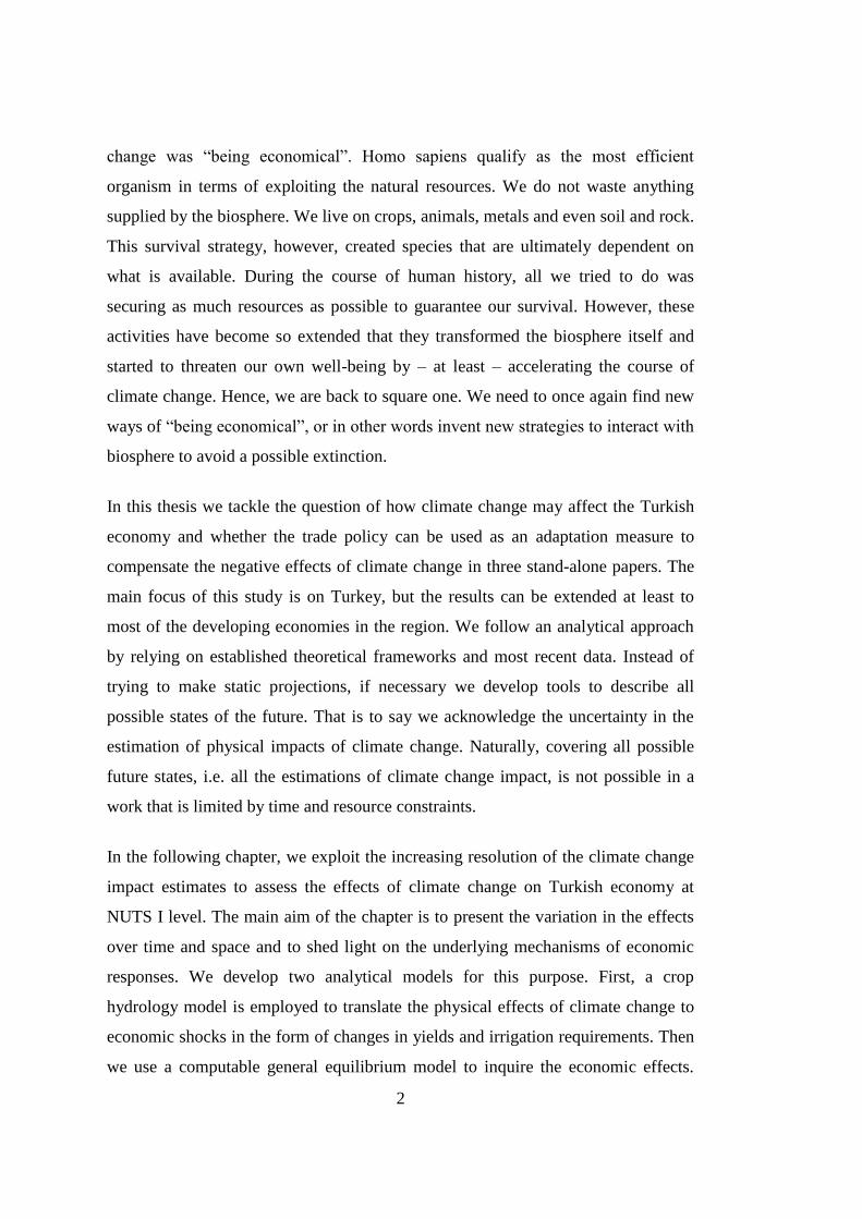
change was “being economical”. Homo sapiens qualify as the most efficient

organism in terms of exploiting the natural resources. We do not waste anything

supplied by the biosphere. We live on crops, animals, metals and even soil and rock.

This survival strategy, however, created species that are ultimately dependent on

what is available. During the course of human history, all we tried to do was

securing as much resources as possible to guarantee our survival. However, these

activities have become so extended that they transformed the biosphere itself and

started to threaten our own well-being by – at least – accelerating the course of

climate change. Hence, we are back to square one. We need to once again find new

ways of “being economical”, or in other words invent new strategies to interact with

biosphere to avoid a possible extinction.

In this thesis we tackle the question of how climate change may affect the Turkish

economy and whether the trade policy can be used as an adaptation measure to

compensate the negative effects of climate change in three stand-alone papers. The

main focus of this study is on Turkey, but the results can be extended at least to

most of the developing economies in the region. We follow an analytical approach

by relying on established theoretical frameworks and most recent data. Instead of

trying to make static projections, if necessary we develop tools to describe all

possible states of the future. That is to say we acknowledge the uncertainty in the

estimation of physical impacts of climate change. Naturally, covering all possible

future states, i.e. all the estimations of climate change impact, is not possible in a

work that is limited by time and resource constraints.

In the following chapter, we exploit the increasing resolution of the climate change

impact estimates to assess the effects of climate change on Turkish economy at

NUTS I level. The main aim of the chapter is to present the variation in the effects

over time and space and to shed light on the underlying mechanisms of economic

responses. We develop two analytical models for this purpose. First, a crop

hydrology model is employed to translate the physical effects of climate change to

economic shocks in the form of changes in yields and irrigation requirements. Then

we use a computable general equilibrium model to inquire the economic effects.

3

Results of the models suggest that the effects can be grouped into three periods.

During the first period, which covers from 2009 to 2035, Turkish economy is not

affected seriously and climate change may even have positive contributions to the

economic activities. The production conditions worsen between 2036 and 2060 with

the increase in the frequency of extreme events. This situation increases the

probability of observing serious adverse effects. Average of the effects is also

worsened. In the last period, from 2065 to 2100, economy is hit hard by the climate

change. Agricultural production is mostly hampered in almost all regions.

In the third chapter, we incorporate the effects under trade liberalization by

developing a recursive dynamic CGE model at the national level. Eliminating the

regional detail from the model allows us to increase sectoral resolution, especially

for agriculture. Both approaches yield similar results related to the impact of

climate change: Amplified effects are observed in the latter two periods, and

agricultural production declines significantly. International trade plays a key role in

the response of the economy to the climate change shocks. Oilseeds and maize turns

out to be the most affected activities. Trade liberalization with EU is found to have

welfare improving effects but these effects are low compared to the harm caused by

climate change. Though the effects increase as climate change effects are worsened.

The main reason is the increase in the substitution possibilities under trade

liberalization.

The last chapter deals with the effects of climate change at the global level. GTAP

model based analysis utilizes a large set of climate change scenarios. The effects of

climate change can now be described by probability distributions. Simulation

results suggest that impact of climate change on global economy spans a large range

of probabilities. The effects are not homogenous for different regions of the world

or for different sectors in a region. On the other hand, the effects of trade

liberalization are generally independent from the assumed climate change scenario.

The results suggest that adverse effects of climate change on welfare can be

alleviated by trade liberalization in most parts of the world. This is especially true

for Turkey where welfare improvement is accompanied by an increase in GDP

4

under full trade liberalization. However, effects of trade liberalization with EU are

again found to be weak.

To sum up, our analysis suggests that Turkey still has time to take necessary

adaptation measures and trade policy can be a policy to contribute to these measures

by removing the constraints on the supply of good for intermediate input use and

consumption. However, results also suggests that trade liberalization cannot cure all

drawbacks of the changing climate by itself. Hence Turkey needs to take more

adaptation measures before it is too late.

5

CHAPTER 2

2. AN INTEGRATED ANALYSIS OF ECONOMY-WIDE

EFFECTS OF CLIMATE CHANGE FOR TURKEY

“Le contraire du simple n'est pas le complexe, mais le faux.”

Andre Comte-Sponville

Effects of climate change in Turkey, which is already a water stressed country, are

expected to be significant. The aim of this chapter is to quantify the effects of

climate change on the overall economy. We use an integrated framework which

incorporates the results of a crop water requirement model in a computable general

equilibrium model for the period 2010-2099. Since agriculture is the most important

sector that will be affected by climate change, analysis of climate change effects on

the overall economy necessitates taking into account backward and forward

linkages to agriculture. The CGE model establishes the links between agriculture,

the other sectors, and also with the economic agents in 12 NUTS-1 regions. A crop

water requirement model is used to translate the results of global climate models to

the changes in yields and irrigation requirements for the period 2008-2099 at 81

NUTS-3 regions for 35 crops. The results of the crop water requirement model are

then introduced to CGE model as climate shocks.

The results suggest that the economic effects of climate change will not be

significant until the late 2030s; which allows Turkey to develop appropriate

adaptation policies. However after 2030s, effects of climate change are significant.

Production patterns and relative prices will change drastically. The economic

effects differ among regions. The effects are milder in the regions where irrigated

agriculture is relatively low. This suggests that climate change policy needs to be

6

region-specific. Agriculture and food production are the most affected sectors.

Increasing irrigation requirements will cause farmers to reduce irrigated production.

Combined with the decline in yields, this will lead to the deterioration of

agricultural production and an increase in agricultural prices. Consequently the loss

in household welfare will be significant. Part of the decline in production can be

compensated by imports, causing an increase in agro-food trade. Trade balance will

worsen with declining manufacturing exports due to increasing cost of production.

In the following sections we will first give a survey of studies related to the effects

of climate change on agriculture and overall economy for Turkey. Then we will

present the modeling approach and the models that are used in this chapter.

Afterwards, we will describe the data used in the models. Results and discussions

will follow. We reserved the last section for concluding remarks.

2.1 Climate Change

A significant effort has been spent by scientists from various disciplines to shed

light on the causes and effects of climate change in recent years (Tol, 2010).

Although there are still some controversies about the details (Idso et al., 2009), it is

widely accepted that the effects of climate change have already started to be felt,

and the significance of the impacts is expected to increase throughout the 21st

century (Agrawala et al., 2008; Parry et al., 2007; Stern, 2006). Although, a wide

range of social and physical effects has been linked to climate change, the most

significant effects are expected to be increasing temperatures accompanied by

declining precipitation, as well as increasing frequency of climatic extremes (Stern,

2006). Hence, agricultural production, which ranks high in terms of climate

dependence, is likely to be the most vulnerable sector (Fankhauser, 2005). The

changes in temperature and precipitation will affect the yields in crop production,

while climate related risks will increase due to increasing frequency of climatic

extremes (Rosegrant et al., 2008).

7

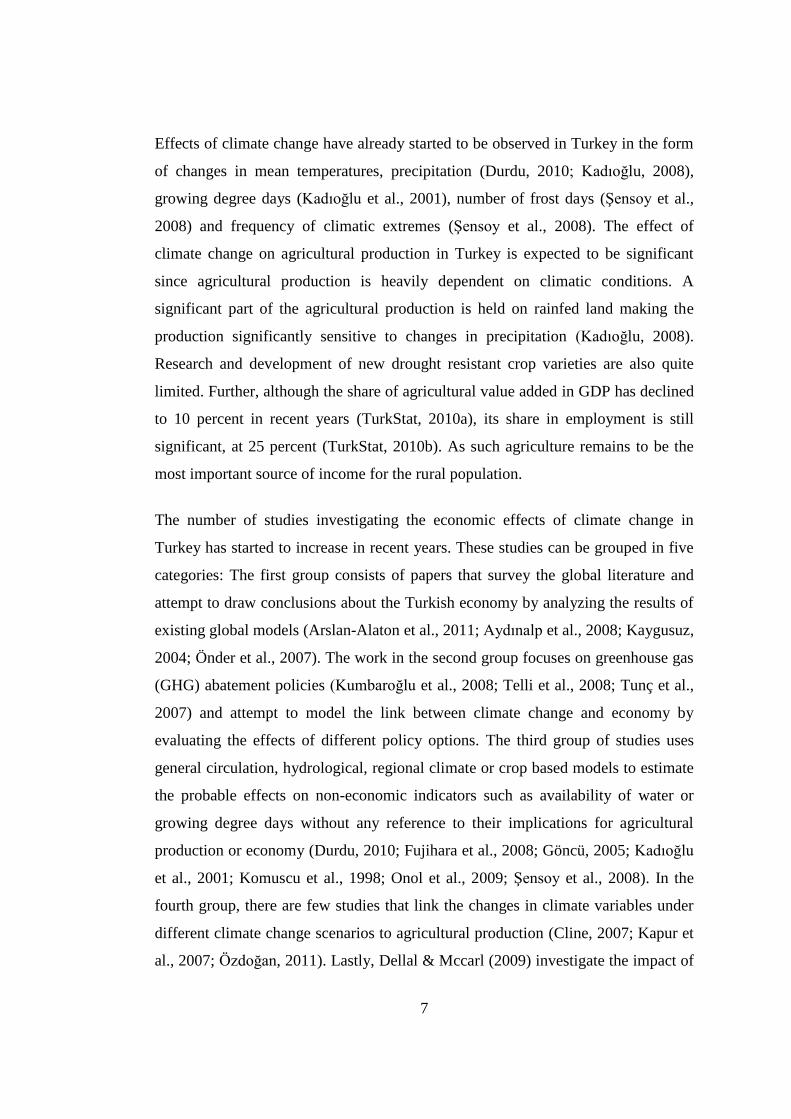
Effects of climate change have already started to be observed in Turkey in the form

of changes in mean temperatures, precipitation (Durdu, 2010; Kadıoğlu, 2008),

growing degree days (Kadıoğlu et al., 2001), number of frost days (Şensoy et al.,

2008) and frequency of climatic extremes (Şensoy et al., 2008). The effect of

climate change on agricultural production in Turkey is expected to be significant

since agricultural production is heavily dependent on climatic conditions. A

significant part of the agricultural production is held on rainfed land making the

production significantly sensitive to changes in precipitation (Kadıoğlu, 2008).

Research and development of new drought resistant crop varieties are also quite

limited. Further, although the share of agricultural value added in GDP has declined

to 10 percent in recent years (TurkStat, 2010a), its share in employment is still

significant, at 25 percent (TurkStat, 2010b). As such agriculture remains to be the

most important source of income for the rural population.

The number of studies investigating the economic effects of climate change in

Turkey has started to increase in recent years. These studies can be grouped in five

categories: The first group consists of papers that survey the global literature and

attempt to draw conclusions about the Turkish economy by analyzing the results of

existing global models (Arslan-Alaton et al., 2011; Aydınalp et al., 2008; Kaygusuz,

2004; Önder et al., 2007). The work in the second group focuses on greenhouse gas

(GHG) abatement policies (Kumbaroğlu et al., 2008; Telli et al., 2008; Tunç et al.,

2007) and attempt to model the link between climate change and economy by

evaluating the effects of different policy options. The third group of studies uses

general circulation, hydrological, regional climate or crop based models to estimate

the probable effects on non-economic indicators such as availability of water or

growing degree days without any reference to their implications for agricultural

production or economy (Durdu, 2010; Fujihara et al., 2008; Göncü, 2005; Kadıoğlu

et al., 2001; Komuscu et al., 1998; Onol et al., 2009; Şensoy et al., 2008). In the

fourth group, there are few studies that link the changes in climate variables under

different climate change scenarios to agricultural production (Cline, 2007; Kapur et

al., 2007; Özdoğan, 2011). Lastly, Dellal & Mccarl (2009) investigate the impact of

8

climate change using a sector model with restricted coverage of agriculture, and

Dudu et al. (2010) try to link climate change projections with the overall economy.

Cline (2007) presents a detailed impact analysis of climate change on 60 countries,

including Turkey, by downscaling the results of five global circulation models.

Cline (2007) reports that the increase in average temperature will be between 1.1°C

and 1.6°C, while average precipitation will decline by 30 percent which translates to

11.8 percent decline in average agricultural yield for the period 2070-2099. This

will result in 16 percent loss in the value added produced by agricultural sector

(Cline, 2007: p.40 and p. 64 and p.71). Cline (2007) also reveals that the initial 1 to

2°C increase in temperature will in fact benefit the agricultural sector. However, the

effects will be reversed when the increase in temperature is higher than 2°C (Cline,

2007, p. 60). The results indicate that estimates of climate change effects for Turkey

have the highest coefficient of variation across different global climate models and

probably are less robust to different model assumptions.

Kapur et al. (2007) attempt to link the climate change effects in Turkey to

agricultural production. They employ a regional climate model to estimate the

effects of climate change on wheat production for the period 2070-2099 under A2

scenario of IPCC in the Çukurova Basin, which is one of Turkey’s most advanced

regions in agricultural production. Their results suggest 35 percent decline in

precipitation accompanied by 2.8°C increase in the mean temperature. However,

they do not report any quantitative results for the probable change in wheat yield.

Recently, Özdoğan (2011) reported the results of a crop model. The impact of

climate change is obtained from a GCM. The study analyzes the effects on wheat

production in the Thrace region. Özdoğan (2011) reports that CO2 effects are likely

to be small and there will be a 15 to 20 percent decline in wheat yield.

Although these studies report the impact of climate change on yields or water

availability, they still do not give much information about the economic effects for

the agricultural sector. Furthermore, these studies also lack spatial and sectoral

depth, in the sense that they merely focus on either the national level or on

9

analyzing specific sub-regions and that they generally limit their analysis to few

major crops.

There are only two well documented studies in the literature that employ economic

models to investigate the implications of climate projections under different climate

change scenarios. Dellal & Mccarl (2009) use a partial equilibrium model for the

agricultural sector to investigate the effects of a climate change on production.

Dudu et al. (2010) on the other hand uses a computable general equilibrium model

to analyze effects of yield changes on the overall economy. Both models suffer

from various deficiencies. In Dellal & Mccarl (2009) the average of results from a

global climate model is used to estimate yield responses. The regional dimension of

the model used is outdated and is not compatible with NUTS classifications of

TurkSTAT. Furthermore the study runs simulations for a limited number of crops.

Dudu et al. (2010), use the average of expected yield changes compiled from

existing literature. The regions chosen are aggregated and they use 2003 social

accounting matrix.

Consequently, there is a need for a more detailed economic analysis of climate

change by combining the results of climate models with economic models at the

regional level. In this chapter, we aim to improve the current modeling efforts in the

literature by using an integrated approach to evaluate the effects of climate change

on the overall economy of Turkey in a detailed regional setting. For this purpose,

we use a crop water requirement model to translate the regionalized results of a

global climate model to yield shocks and irrigation requirement changes. These

changes are introduced as productivity shocks to a CGE model. The following

section presents the modeling approach for the CGE model in detail and the crop

water requirement model. Section 2.3 presents the data and aggregated results of

crop water model. The results of CGE analysis are discussed in Section 2.4 reports.

The last section is reserved for the concluding remarks.

10

2.2 Integrated Modeling Approach

Climate change is a complex issue and any complete assessment of its effects needs

to take into account the interactions of physical, economic and social factors.

Consequently, a comprehensive impact assessment requires different types of

models. Complicated climate and hydrology models are needed to estimate the

physical effects at the global level. The estimates from these models then need to be

downscaled to smaller spatial resolutions to obtain the effects at the regional level.

In addition, the interaction within an economy and the rest of the world needs to be

considered in detail to have a solid interpretation of the economic effects. As

mentioned before, climate change is expected to affect the economy via the

agricultural sector. Hence, a special impact assessment model is required to link the

results of climate models to the economic models. Therefore, complete impact

analysis of climate change necessitate to integrate physical models, specific impact

assessment models and economic models.

This “three pillar” approach has started to dominate the literature recently supported

by the availability of disaggregated climate change data and by the increasing

computational power. Global Circulation Models (GCMs) are now used extensively

to make projections related to the main climatic variables under different scenarios.

Although the results of these models are controversial, especially at the regional

level, the mean values of the results from many available GCMs are used as a

proxy. The type and specification of special impact models used to translate GCMs

output to economic impacts differ according to the aim of the study. Lastly,

computable general equilibrium modeling has become the standard approach to

estimate the economic effects.

There is vast literature related to the agricultural and economy-wide effects of

climate change. The literature survey here will be selective by considering the

studies that adopted similar approach to the one adopted in this chapter. More

comprehensive surveys on the integrated approach can be found in Hertel & Rosch

(2010) and also in Palatnik & Roson (2009).

11

In their study Bosello & Zhang (2005) use a GCM that combines a crop- growth

model with a global CGE model (GTAP-E). The climate scenario is endogenously

produced by the economic model. The results indicate that climate change has a

limited impact on agricultural sectors mainly due to the smoothing effect of

economic adaptation. Bosello & Zhang (2005) are separated from the other studies

since they report insignificant effects on agriculture.

Rosegrant et al. (2008) and Nelson et al. (2009) use a global food supply and

demand model (IMPACT) together with a biophysical model (DSSAT) to estimate

the impacts of climate change on agriculture at the global level. They report that

climate change will affect human well-being negatively due to declining yields and

increasing prices. Calorie availability will be worsened and child malnutrition will

increase by 20 percent. They estimate that USD1.7 billion in 2000 prices is needed

to offset the effect of climate change on calorie availability.

Cretegny (2009) develops a conceptual framework that uses an integrated approach

at national and global level. The study presents an implementation of bottom-up and

top-down approaches for integrated modeling of climate change. In the bottom-up

methodology, the projected changes in climatic variables obtained from multiple

GCMs are first downscaled to local levels, and then they are used to estimate the

vector of impacts on key economic sectors using sector-specific impact assessment

models. In the top-down methodology, the climate projections are used to derive

regional sector-specific damage functions that are used to calibrate a global

dynamic multi-sectoral CGE model.

Thurlow et al. (2012) investigate the effect of climate variability and climate change

on Zambian economy by using a hydro-crop model (CropWAT model of FAO) for

maize in Zambia together with a dynamic CGE model. They use historical climatic

data and HadCM3 results from a hydro-crop model to obtain yield responses of

maize under different drought and climate change scenarios. They estimate yield

losses up to 50 percent in years with severe drought. The results of CGE model

suggest that climate variability may result in USD4.3 billion losses over a 10-year

12

period, leaving 300,000 people below the poverty line. Climate change effects add

another USD2.15 billion to the losses; pushing 74,000 more people below poverty

line.

Ciscar et al. (2009) use various impact assessment models with a CGE (GEM-E3)

model. Most EU countries are modeled individually in the CGE model. DSSAT

crop models have been used to quantify the physical impact on agriculture. Their

findings suggest that most European regions would experience yield improvements

during the 2020s, but in the 2080s average crop yield will fall by 10 percent.

Southern Europe would experience relatively higher yield losses. They estimate that

annual damage of climate change to the EU economy in terms of GDP loss will be

between €20 billion to €65 billion implying 0.2 percent and one percent welfare

loss, respectively.

Pauw et al. (2010) use a general equilibrium model to estimate the economy wide

impact of production losses due to hydrological extremes in Malawi. Climate

simulations are based on production loss estimates from stochastic drought and

flood models. Results show that 1.7 percent of GDP will be lost due to climate

change, small farmers will be affected more prominently, and food shortages are

likely to affect urban households significantly.

Calzadilla et al. (2011) investigate the impact of variation in water availability due

to climate change on the global agricultural production. They use a multi-sectoral

global CGE model (GTAP-W) and a Global Environmental Model, which includes

a dynamic river routing model (HadGEM1-TRIP), to simulate changes in

temperature, precipitation and river flow over the next century under the IPCC

scenarios. They report that global food production, welfare and GDP will decline.

Food prices are expected to increase. They also show that countries are not only

influenced by regional climate change, but also by climate-induced changes in

competitiveness in the global markets.

Fernandes et al. (2012) use an agro-ecological model together with an applied

general equilibrium model (ENVISAGE) to assess the impact of climate change in

13

Latin America. The agro-ecological model consists of crop development, soil types,

water availability, abiotic factors, management and crop suitability components.

The results suggest that there will be significant decline in the yields of major crops

and the effects will be higher after 2050. Adaptation is partially effective in off-

setting the climate change effects. Economic impacts are also significant, adding up

to 1.3 percent decline in region’s GDP.

All studies share two common findings. First is that climate change effects on the

overall economy and particularly on agricultural production may be significant,

especially for developing countries where the share of agricultural value added in

GDP is high. Secondly, the effects accelerate in the second half of the 21st century,

especially for developed countries. The results are region and crop specific, and

aggregation at any level underestimates the effects. Adaptation policies can be

effective to lessen the economic losses.

The modeling approach used in this Chapter follows the three pillar approach

presented in Figure 2.1. We use the output of a GCM as an input for the crop water

requirement model to estimate the yield and irrigation water requirement of

different crops. Then the output of the crop water requirement model is used as an

input for the CGE model in the form of productivity shocks. Details of the modeling

structure are provided in the next two sections.

14

Figure 2.1: Summary of modeling approach

2.2.1 Crop Water Requirement Model

The physical effects of climate change on agricultural commodity production are

generally assessed by using hydrology and crop simulation models. These models

take the forecasts of the major climatic variables, i.e. precipitation, temperature and

wind speed, from the global circulation models (GCM), and use them to calculate or

estimate the induced yield changes. The aggregated results obtained from the crop

water requirement model are presented in this section and the detailed description of

the model can be found in Appendix A. The estimated changes in yields and

irrigation requirements are then introduced to the CGE model as climate change

shocks.

The average value of (the reference evapotranspiration) is presented in Figure

2.2. increases slowly until 2060. However the oscillation around the mean

0ET

0ET

CG

E M

odel

Hydro

-crop

Mo

del

Clim

ate Model

Precipitation

Change

Climate Change

Temperature

Change

Water Stress

Yield Change

GHG Emissions

Agricultural Production

Rest of the economy

Water Supply

Irrigation Requirement

15

value increases significantly between 2035 and 2060. Significant rise in the pace of

increase in is observed from 2060 to 2075, and the variation in remains

high after 2075.

Source: Author’s Calculations

Figure 2.2: Change in reference evapotranspiration (percentage change with

respect to base period)

We use the change in yields for 35 crops (for details see Appendix A) to calculate

the change in agricultural value added relative to the production value of

agricultural products in 2008 for each NUTS-3 regions. Then, we aggregate the

results at NUTS-1 regions by using the following formula:

, 3 , 3 , 3

1 3 1, 3 , 3

. .

.

c R c R c RcR R R

c R c Rc

Y P QVA

P Q

(2.1)

where is the change in yield, is the price, is the production

quantity of crop c in NUTS-3 region R3.

0ET 0ET

, 3c RY, 3c RP , 3c RQ

16

Monthly irrigation requirements for each crop in each region and year are calculated

as the deficiency between precipitation and . Area of cultivated land in 2008 is

used to find a weighted sum of the total irrigation for each NUTS-1 region, and also

to determine a region-wide irrigation requirement per hectare.

, 3, , 3, , , 3,20083 11,

, 3,2008

C R M Y R M Y C RR R C MR Y

C RC

ETS PR AIRQ

A

(2.2)

where is evapotranspiration of crop C under water stress in region R3,

month M and year Y. is the effective precipitation in region R3, month M

and year Y. is the harvested area of crop C in region R3 in 2008.

The change in the irrigation water requirement is calculated relative to the average

irrigation water requirement for the period 2001-2010.

1,

1, 2010

, 1,

2001

10

R Y

R Y

C R B

B

IRQIRQ

IRQ

(2.3)

Figure 2.3 displays the estimated changes in yields and irrigation water

requirements from 2001 to 2099. The changes in yields and water requirements

follow slightly different trends than . Yield changes oscillate less in comparison

with water requirements, which is highly dependent on precipitation. Both figures

oscillate around base decade values until 2035. After 2035 the yields start to decline

while irrigation requirements start to increase. Consequently, increase in irrigation

requirements and decline in yields become significant after 2060. Lastly, note that

variation in yields and irrigation requirements are significantly higher than the

variation in

sET

, 3, ,C R M YETS

3, ,R M YPR

, 3,2008C RA

0ET

0ET

17

Source: Author’s Calculations

Figure 2.3: Average yield change and irrigation water requirement

A more accurate way to look at these yield changes is considering them as drawn

from a probability distribution. In that case climate change will affect the mean and

standard deviation of the distribution of yield changes. Effects on the economy for

each period will also be drawn from a probability distribution. Figure 2.4 shows the

estimated probability density1 of the yield shocks for the periods mentioned above.

The distribution of yields shifts to the left indicating lower means for the yield

shocks. The spread of the distribution, which is related to the climate risk, is also

higher in the second and third period compared to the first period. In the first period

the distribution is centered on zero median and almost zero mean with extreme

1 Kernel density estimation graphs are used to visualize this approach. Kernel density estimations are

smoothing methods to estimate the probability density function. We follow the methods developed

in Silverman (1992) to estimate the probability distributions from the model results.

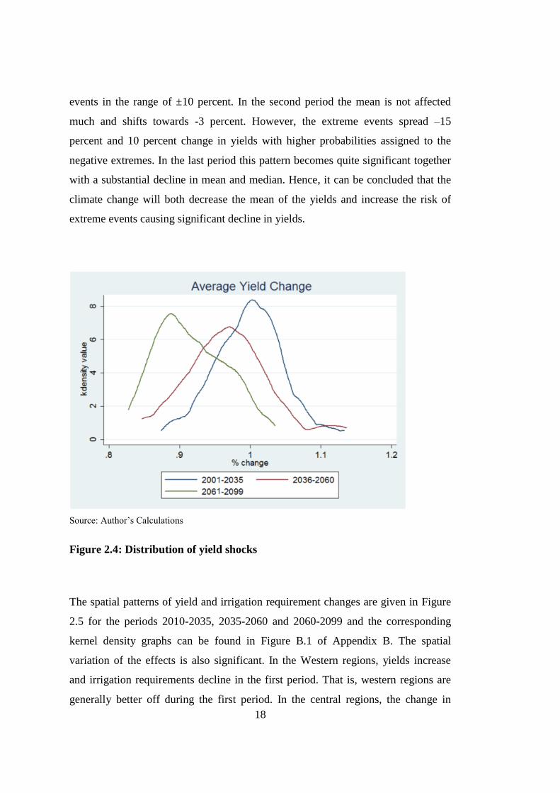
18

events in the range of ±10 percent. In the second period the mean is not affected

much and shifts towards -3 percent. However, the extreme events spread –15

percent and 10 percent change in yields with higher probabilities assigned to the

negative extremes. In the last period this pattern becomes quite significant together

with a substantial decline in mean and median. Hence, it can be concluded that the

climate change will both decrease the mean of the yields and increase the risk of

extreme events causing significant decline in yields.

Source: Author’s Calculations

Figure 2.4: Distribution of yield shocks

The spatial patterns of yield and irrigation requirement changes are given in Figure

2.5 for the periods 2010-2035, 2035-2060 and 2060-2099 and the corresponding

kernel density graphs can be found in Figure B.1 of Appendix B. The spatial

variation of the effects is also significant. In the Western regions, yields increase

and irrigation requirements decline in the first period. That is, western regions are

generally better off during the first period. In the central regions, the change in

19

yields is generally small with lower irrigation requirements. The eastern parts, on

the other hand, are likely to experience an increasing water requirement and slight

declines in the yields starting from the first period.

Change in Yields Change in Irrigation Requirements

Source: Author’s Calculations

Figure 2.5: Spatial effects of climate change

In coastal zones, central regions and eastern parts of the country, the effects of

climate change differ significantly in the second period. In the coastal regions, yield

changes are not significant, except in the Thrace, and irrigation requirements

increase slightly. Eastern parts of the country become slightly worse off with lower

yields and higher irrigation requirements. However, Central regions are heavily

affected from of climate change. Average yield loss exceeds 10 percent for some

20

provinces, while decreasing trend in irrigation water requirements in the first period

is completely reversed.

The difference in the effects of climate change becomes significant in the north-

south axis, rather than the east-west axis. Furthermore, although the changes in

yields and irrigation requirements follow approximately the same spatial pattern in

the first two periods, they follow completely different patterns in the third period.

The provinces that suffer from high yield loss form a belt like shape starting from

Thrace, extending through the northern parts of the central regions and ending in the

central parts of the eastern regions. The increase in the irrigation requirement is

higher in the Northern regions, especially in the central regions and Thrace.

Our results support the findings of the other studies in the literature, both at the

national and global level. The effects become more significant after 2060s.

Furthermore, the effects are significant for all periods in some regions. Results also

show that the variation in yields is higher than the variation in climatic conditions.

This suggests that agricultural production is more prone to climatic changes and

risks related to it. Lastly, as predicted by many studies the technical conditions

become more favorable for agricultural production at the early stages of climate

change when the increase in the mean temperature is below 2°C.

2.2.2 Regional CGE model

The Walrasian CGE model developed in this chapter disaggregates the economy

into seven activities producing commodities for seven sectors in each of the 12

NUTS-1 regions. The activities are agriculture, food production, textiles, other

manufacturing, energy, public services and private services. The production

structure of the activities is presented in Figure 2.6. We use a three level nested

production function which aggregates different factors and inputs at different levels.

21

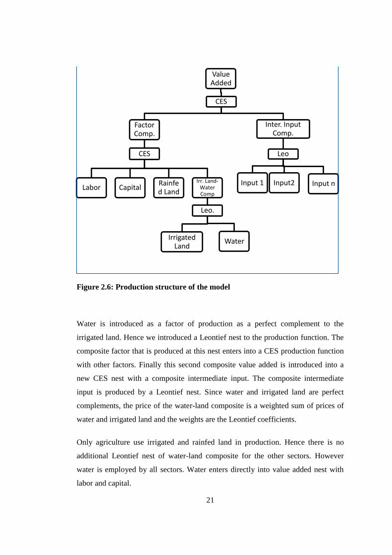
Figure 2.6: Production structure of the model

Water is introduced as a factor of production as a perfect complement to the

irrigated land. Hence we introduced a Leontief nest to the production function. The

composite factor that is produced at this nest enters into a CES production function

with other factors. Finally this second composite value added is introduced into a

new CES nest with a composite intermediate input. The composite intermediate

input is produced by a Leontief nest. Since water and irrigated land are perfect

complements, the price of the water-land composite is a weighted sum of prices of

water and irrigated land and the weights are the Leontief coefficients.

Only agriculture use irrigated and rainfed land in production. Hence there is no

additional Leontief nest of water-land composite for the other sectors. However

water is employed by all sectors. Water enters directly into value added nest with

labor and capital.

Value Added

CES

Factor Comp.

CES

Labor Capital Rainfed Land

Irr. Land-Water Comp

Leo.

Irrigated Land

Water

Inter. Input Comp.

Leo

Input 1 Input2 Input n

22

There is only one type of household in each region. Income generated by factors in

a region is distributed to the household in the same region. Households receive

income from labor, land and water, while capital income goes to firms. From this

income, firms pay institutional taxes, make transfers to the rest of the world, and

distribute the remainder to households together with the transfers from the

government. Households use their income for consumption, leisure, savings and

taxes. Households maximize a Linear Expenditure System (LES) utility function to

make consumption decision. Leisure enters the utility function like any other

commodity, while the wage income is included as a budget constraint. The utility

maximization problem is:

, 0 , 0, , , , , , ,

1

, , , , , , , , , , ,

1

max ln ln

. .

k

r h r h r h r i i r h i r h

i

k

r i r i r h r h r h r h r h r h r h r h r h

i

U L QH

s t P QH w L EH w L w T YNL Y

(2.4)

where the indice i denotes commodities, r denotes regions and h denotes the

households. is household demand for commodity i, is labor supply,

is unemployment, is leisure, is commodity prices, is wage rate of

labor, is total consumption spending of the households, is the total

number of working age individuals in a household. is non-labor income,

is total income. The above formulation suggests that households decide how many

people should work to earn wages and how many of them are reserved for leisure.

Unemployment is determined in the labor market as the difference between labor

supply and labor demand. We assume that households neither receive leisure nor

wages for unemployed people.

The analytical solution of this problem yields the following demand functions:

, ,

, , , , , , , ,

10, , ,1

ki r h

i r h i r h r h i r i r h

ir h r i

QH EH PP

(2.5)

, ,i r hQH ,r hQFS

,r hU ,r hL,r iP ,r hw

,r hEH ,r hT

,r hYNL,r hY

23

0, ,

, , , 0, , , , , ,

10, , ,1

kr h

r h r h r h r h r h r i i r h

ir h r h

QFS U T EH Pw

(2.6)

In the above equations, is the total working-age population and it is not

adjusted for wages since household cannot control the total population or the

parameter . Hence, following Thurlow (2008), we introduce the following “rule

of motion” for total available working-age population:

,, , 0, , ,

, , 0, , ,

r tr h t r h t t

r h b r h b b b

wfr cpiT

T wfr cpi

(2.7)

where the t denotes a post-simulation values and b denotes the base run values,

is wage rate and is the consumer price index. Accordingly, an increase in real

wage rate increases the total available working age population, and vice versa.

Government receives tax income from activities, commodities, firms and

households as well as transfers from the rest of the world. This income is used for

government consumption, transfers to households and firms, government savings

and transfers to the rest of the world.

Production activities make payments to commodity accounts for intermediate

inputs, to factors such as wage payments and to government as net taxes. They

receive payments from commodity accounts in exchange for supply of goods and

services. Commodity accounts also make payments to the rest of the world for

imports and to government for indirect taxes. They receive payments from

households for consumption of goods and from the rest of the world for exports.

Model closure rules follow conventional neoclassical assumptions. Since

simulations are designed to account for the long run climate change effects, it is

assumed that the price of capital and land is fixed while their supply and demand

adjust to the new equilibrium. Water is assumed to be fully employed and mobile

, 0, ,r h r hT

,r hT

0, ,r h

wfr

cpi

24

among activities within a region and its supply is fixed. Demand for water adjusts to

the new equilibrium. Consumer price index is the numéraire and hence is fixed

while domestic producer price index adjusts to clean the markets. We use a

balanced closure rule for saving-investment market. Investment is a fixed share of

absorption and marginal propensity to save is scaled to equalize savings and

investments. Exchange rate is fixed by allowing foreign savings to adjust to keep

the current account at balance. The share of government demand in total absorption

is also fixed. Lastly, government savings are fixed, while direct tax rates are flexible

and are scaled for households and firms to sustain the balance of government

accounts. Further discussion of closure rules can be found in Lofgren, Harris, &

Robinson (2003).

2.3 Description of Data and Simulations

The aggregate version of the SAM (Social Accounting Matrix) used in the analysis

follows from Yiğiteli (2010) who presents a national SAM of the Turkish Economy

for the year 2008. The SAM developed by Yiğiteli (2010) consists of 49 production

activities which produce 49 commodities using formal and informal labor, land and

capital. It has five household types differentiated according to income groups. We

used various data sources to regionalize the 2008 National SAM into 12 NUTS-1

regions.

The I/O table used in this model is a regionalized version of 2002 I/O table that is

published by TurkSTAT (2011a). Augmented Flegg Location Quotients method

(Flegg & Webber, 2000) is used to regionalize the 2002 National I/O table by using

regional data on employment. The latest regional employment data available for all

sectors of the model is for 2002. Hence the shares of each region in each sector are

used to interpolate 2008 employment figures across regions. These employment

figures are in turn used in AFLQ formula as described in Flegg & Webber (2000):

25

2 2

,

2

log 1 log 1 1

log 1 1

R RR R RR Rj ji i ii j ji i

N N N N N N N

i j i j j i ii j iR

i jR R RR R

i i ii j i i

N N N N N

i j i i ii i

E EE E EE Eif

E E E E E E EAFLQ

E E EE Eif

E E E E E

(2.8)

where is employment in sector i of region R, and is national employment in

sector I, while is a constant assumed to be 0.3 following Flegg & Webber (2000).

that denotes the element of I/O table in ith row and jth column, is calculated as:

, , ,.R N R

i j i j i ja a AFLQ (2.9)

where is the national I/O share.

After calculating new regional I/O shares further adjustments are made in the SAM.

Firstly, the regional coefficients do not necessarily add-up to one for an activity in a

region, that makes I/O table imbalanced. To keep the balance of I/O columns, it is

assumed that the deficiency (or excess) in the row sum of regional I/O table is due

to the missing intermediate input trade among regions. Hence intermediate input

trade among regions that make I/O table consistent is calculated by assuming that

the intermediate input flow from one (exporting) region to another (importing)

region is proportional with the share of exporting region in national production.

Secondly, the row sums of I/O table do not necessarily add up to regional

production figures. Hence regional production figures are adjusted according to new

I/O table. The imbalance in the commodity accounts, which is caused by this

operation, is in turn balanced by introducing inter-regional trade.

Interregional trade is the key economic link among regions. Since the data on

interregional trade is scanty, it is calculated for the purpose of this analysis. The

discrepancy between the production and consumption of a region needs to be

supplied by other regions to keep the SAM balanced. In doing so, it is assumed that

R

iE N

iE

R

ija

N

ija

26

every region's supply of commodities to the other regions is proportional to the

former's share in the national production. That is to say, differences in

transportation costs among different regions are ignored. Regions where production

exceeds consumption are assumed to consume only their own products and export

the remainder to other regions. For importing regions, the imported amount is

subtracted from the region's production to keep the balance between consumption

and production. In other words, we assume that interregional trade is done among

producers of exporting and importing region and wholesalers of importing region.

Hence value added produced in a region also includes the value of commodities

obtained by trade. A better alternative would have been introducing interregional

trade through households but due to lack of data this option is not viable for the

current model.2

The need for intermediate input and commodity trade among regions can be

elucidated with an example. Istanbul, namely TR1, is characterized by high

industrial employment and production with small agricultural employment and

production. However, the consumption of agricultural products is significantly

higher than the production in Istanbul due to the population size. It is impossible to

satisfy the consumption in Istanbul with its own production. Hence, the discrepancy

in regional supply and demand is assumed to be supplied by other regions,

according to the share of the latter in national production. That is, a region with

higher agricultural production supplies more agricultural commodities to Istanbul.

The need for interregional trade in intermediate goods can also be explained in the

context of agricultural production in Istanbul. Istanbul has a high share in

2 This interregional trade is neutral in the sense that, we do not introduce any behavioral assumption

for wholesalers. They only transport the goods of the importing sector to the suppliers of exporting

sectors and there is no transaction cost in the process. Further, we also assume that the commodities

from different regions are perfectly substitutable.

27

manufacturing production and hence an important part of agricultural inputs is

produced in Istanbul. However, since Istanbul produces small amounts of

agricultural products either the intermediate input use of agricultural sector in

Istanbul needs to be unrealistically high or some of the intermediate inputs need to

be exported to the other regions. The distribution among regions is again

proportional to the production of the exporting region. By following this logic we

create a bilateral intermediate input and commodity trade matrix.

The value added for water is calculated from the rent differentials obtained from the

Quantitative Household Survey (QHS) held by the G&G Consulting et al. (2005).

Data for the 1,356 farm households are used to calculate the rent for irrigated and

rainfed land at NUTS-1 level. Average rental rate per ha. in 2004 is projected to

2008 by assuming that the change in rent would be same as the change in wholesale

price index for agricultural sector which is approximately 32 percent between 2004

and 2008. The difference between the rental rate of irrigated land and rainfed land

was attributed to the irrigation, and hence that difference was used as the price of

water. The value added of water in agricultural sector is calculated by multiplying

the rent difference with the area of irrigated land. The payments from other sectors

to water factors are calculated from TurkSTAT Municipality Water Statistics

(TurkStat, 2011a).

Regional employment shares for each sector are obtained from the Annual Industry

and Services Statistics (TurkStat, 2011b). Then, national employment figures

reported in Regional Household Labor Force Statistics (TurkStat, 2011c) for each

sector are distributed to the regions by using these shares. Total working-age

population is based on the number of people between 14 and 65 years of age.

Regional unemployment figures are also obtained from the Regional Household

Labor Force Statistics (TurkStat, 2011c).

The regional disaggregation of the trade figures was done by using TurkStat’s

Regional Foreign Trade database for 2008 (TurkStat, 2010c). Agriculture, energy,

manufacturing and services are disaggregated directly by using the shares of regions

28

in the trade of these sectors. Regional trade data for food and textiles are not

available. Hence trade figures of regions are adjusted by taking into account the

region’s share in the national production of the relevant sector and region's share in

the trade of manufacturing. The formula used is as follows:

Q R Q R

R R

R RR

S R S R

S R R

R R

X Y

X Y

X Y

X Y

(2.10)

where R is the regional share, is a region’s production in the sector and is

volume of the region’s trade in manufacturing. Shares that are less than one percent

are ignored. For imports, region’s share in manufacturing trade is directly used for

adjustment.

Yiğiteli (2010) assumed a constant rate of tariff for all commodities. Tariffs are

recalculated from the average applied tariff rates at HS6 level for 2008 (Ministry of

Customs and Trade, 2011).

Consumption is disaggregated according to TurkStat (2010b) which reports

distribution of household consumption according to regions and income quintiles.

Households are not allowed to consume commodities from other regions.

Government consumption is distributed according to the 2008 Public Accounts

Bulletin (General Directorate of Public Accounts, 2010a). Government

consumption in each sector is distributed according to the region's share in total

government expenditures on goods and services purchases. Transfers are also

distributed according to 2008 Public Accounts Bulletin (General Directorate of

Public Accounts, 2010b). On the other hand, investments in different sectors are

distributed according to region's share in value added.

Factor incomes are distributed according to the regions' shares in factor value

added. However since capital income is distributed to the regional firms, an

X Y

29

adjustment is made in the capital account to keep the balance of SAM intact. Firm

income is then distributed to households as rent income, government as taxes and

rest of the world as transfers abroad. The imbalance in the firm account is balanced

by increasing the government transfers to the firm. Since this difference is generally

small, the balancing procedure is not likely to affect the model results.

Profit transfers to abroad and workers’ remittances from the rest of the world are

distributed according to the regions’ shares in the national capital income3. The

number of people receiving pensions per region, as reported by Social Security

Institution Yearbook 2008 (Social Security Institution, 2010) is used to distribute

the transfers from SSI to households. Other transfers from government to

households are distributed according to each region’s share in the total transfers as

reported in the Social Assistance and Solidarity Fund (2010). Government savings

and payments to ROW made by government, as well as tax incomes of government

are not distributed since these accounts are national. Tax payments of domestic

institutions are distributed according to data reported by General Directorate of

Public Accounts (2010a). Regions' shares are calculated using accrued tax amounts.

Some minor adjustments are done in the SAM to eliminate very small trade figures

that appear in the energy trade of the North Western and Central Regions as well as

food trade of the Eastern regions. Small exports are added to the S-I account. Import

taxes are deducted from S-I account. A similar adjustment is done for interregional

trade. Accordingly, small interregional trade is eliminated by moving these figures

to the production of consuming regions. Then the difference is added to the S-I

account. The sum of moved figures are added to the government savings accounts

and discounted from the transfers made to the government from the rest of the

3 The method of distribution of remittances from abroad does not have a significant effect on the

model, since the share of remittances in household income is only about 0.2 percent.

30

world. I/O table is also adjusted for small figures. Small figures flowing from

agriculture to energy and to private and public service commodities are added to the

labor value added. The increase in the income generated by the labor is distributed

to households. Then the household consumption is increased respectively to balance

the commodity accounts.

The climate change scenario is simulated by simultaneously shocking the average

yield and irrigation water requirements at NUTS-1 level. One important caveat

about simulations is that they are static experiments derived from annual changes

and hence the results lack any dynamic feedback effects.

2.4 Results and Discussion

Simulation results suggest that the effects of climate change on economy will be

quite significant4. Table 2.1 shows the effect of climate change on main

macroeconomic variables. Welfare indicators such as absorption and household

consumption do not change significantly in the first period, but worsen in the

second and third periods. The change in the second period is likely to be caused by

the years with extreme conditions, while the changes in the third period are due to

decline in the average technical conditions of agriculture. Although the maximum

values are close to the first period, the minimum values are significantly lower. This

implies that the effects of climate change in the second period may be essentially

attributed to the “bad” years due to extreme climatic events, which in turn affect the

economy adversely. In the third period, the negative effects become considerably

higher, with vast declines in maximum values and relatively small declines in

minimum values. This suggests that in the third period, the effects of climate

4 We run statistical tests to see if the mean and variance of the total production differs across the

periods. Difference between the average changes in the production value of all sectors among

periods is statistically significant at 5 percent significance level.

31

change will not only be felt through the extreme events but the average conditions

will also worsen. The effect on the foreign savings and the ratio of other macro

indicators to the GDP is insignificant. This implies that the change in these

indicators is parallel to the change in GDP.

Table 2.1: Effects on selected aggregate variables (base values at billion TL)

Base Percentage Change

Level 2010-2035 2036-2060 2061-2099

Billion TL. Min. Avg. Max Min. Avg. Max Min. Avg. Max

Rea

l

GDP 843.6 -6.46 0.10 5.96 -8.02 -1.39 5.99 -9.72 -3.99 1.70

Absorption 996.4 -6.13 0.08 5.56 -7.61 -1.33 5.60 -9.25 -3.78 1.57

Household Cons.

688.9 -6.59 0.09 5.98 -8.20 -1.43 6.00 -9.96 -4.06 1.70

Export 227.2 -6.14 0.08 5.89 -7.66 -1.39 5.86 -9.20 -3.83 1.57

Import 269.3 -5.18 0.07 4.97 -6.46 -1.17 4.94 -7.76 -3.23 1.32

Real Exch. Rate

100 -0.28 0.01 0.28 -0.37 -0.08 0.29 -0.40 -0.18 0.10

Dom. Price Ind.

100 -2.54 -0.01 2.11 -3.19 -0.57 2.17 -3.92 -1.59 0.48

Rati

o t

o G

DP

Investment 22.23 -0.03 0.00 0.04 -0.03 0.01 0.05 -0.01 0.02 0.06

Private Saving

15.08 -0.31 0.00 0.27 -0.39 -0.07 0.26 -0.49 -0.19 0.08

Foreign Saving

5.24 -0.19 0.00 0.22 -0.19 0.05 0.27 -0.06 0.13 0.33

Trade Deficit

6.62 -0.16 0.00 0.19 -0.16 0.04 0.24 -0.06 0.11 0.30

Gov. Saving 1.91 -0.11 0.00 0.14 -0.11 0.03 0.17 -0.03 0.08 0.21

Source: Author’s calculations

The risk associated with the climate change is illustrated by the spread of change in

GDP over three periods in Figure 2.7. Risk is relatively low with a mean and

median around zero and higher probabilities assigned to relatively small changes in

the first period. Hence the probability of observing a positive growth is high. In the

second period, although the mean and median of the distribution do not change

considerably, the probability assigned to the tails increases. Thus the probability of

observing a negative change increases substantially. Finally, in the third period, the

32

mean and median shift to -5 percent while the spread increases. Hence, in the third

period the probability of observing a positive change in GDP is very small.

Consequently, climate change does not only decrease the average growth rate but

also increase the frequency of extreme events. This has quite significant

implications for the climate policy. Adaptation under these circumstances implies

reducing the adverse effects not only in the average but especially in negative

extreme years. Hence this fact should be taken into account when making the cost

benefit analysis for adaptation.

Source: Author’s calculations

Figure 2.7: Distribution of nominal gross value added

Table 2.2 shows the change in household income. The average change in the

household income is small for the first period while it becomes significant in the

following periods. The difference between the average values gets wider in the

second and third period. Furthermore, the maximum and minimum values of the

change in the household income differ significantly across regions. Accordingly,

incomes of the households in the western and central regions are more sensitive to

33

the extreme climatic conditions. This is mainly due to significant decline in the

prices of the factors that are more often employed by these regions, since the prices

of capital and land are fixed and the share of water in the total income is quite

small, the changes in household income are mainly driven by wages. The change in

wages is in turn driven by the ability of firms to substitute water with labor in the

non-agricultural sectors and with water-land composite in agriculture. Accordingly,

the substitution is limited in Thrace, central Anatolia and eastern regions due to the

low water use in the base year. These regions benefit from the increase in the water

price since income generated by water goes to households. This brings about an

important feedback effect. The increase in the demand for water will drive the price

of water up and this will compensate the loss in household welfare due to

decreasing wages in the mentioned regions.

Table 2.2: Household income according to regions (base values at billion TL)

Base Percentage Change

Level 2010-2035 2036-2060 2061-2100

million TL. Min. Avg. Max. Min. Avg. Max. Min. Avg. Max.

TR1 212,394 -11.13 0.13 10.44 -13.80 -2.50 10.45 -16.49 -6.90 2.67

TR2 41,916 -3.94 -0.14 4.21 -2.20 0.09 2.04 -3.95 -0.04 2.66

TR3 117,556 -7.71 -0.15 6.58 -9.65 -1.87 7.36 -11.60 -4.98 1.36

TR4 87,828 -7.86 0.10 7.25 -9.82 -1.71 7.39 -11.81 -4.92 1.73

TR5 89,146 -8.28 0.09 7.64 -10.32 -1.81 7.73 -12.52 -5.16 1.78

TR6 100,333 -5.74 0.10 5.35 -7.17 -1.18 5.54 -8.88 -3.61 1.30

TR7 38,343 -2.35 0.15 3.63 -2.32 0.17 2.81 -3.38 -0.45 1.45

TR8 46,688 -4.32 0.06 3.93 -4.70 -0.98 3.07 -5.57 -2.30 2.77

TR9 29,798 -2.80 0.05 2.82 -3.72 -0.80 2.26 -4.45 -1.92 0.19

TRA 21,083 -2.37 0.75 5.55 -3.46 0.69 5.44 -3.53 2.17 7.93

TRB 35,165 -1.02 0.88 3.41 -2.49 1.54 3.78 -1.10 2.94 6.05

TRC 70,180 -1.35 0.00 1.03 -1.43 -0.22 1.10 -2.01 -0.80 0.81

Turkey 890,431 -6.18 0.10 5.73 -7.66 -1.33 5.76 -9.28 -3.81 1.61

Source: Author’s calculations

Climate change affects all sectors significantly, although the shocks are introduced

only to the agriculture. This is a result of complex interactions among the sectors.

The significant change in food production can be explained by the fact that

agricultural commodities are important intermediate inputs for this sector. However,

34

this is not the only linkage between the sectors. All sectors compete for factors and

hence a change in the factor demand in one sector affects all sectors. Secondly, the

sectors also interact in the commodity markets. Since all commodities are

substitutable in household demand, a change in the price of one commodity affects

the demand for other commodities as well. Table 2.3 reports the state of commodity

and factor markets. Details for the rest of the sectors can be found in Appendix

Table B.1. The average changes in the markets are not significant for the first

period. There is a slight increase in production and consumption of all commodities

while prices remain almost constant. The most important changes in international

trade are observed in agriculture, food and textile trade. Agricultural trade increases

significantly due to the increase in exports. Despite the slight increase in imports,

the trade balance improves.

Food and textile sectors follow the same trend where exports increase more than

imports. Imports and exports in the other sectors do not change significantly. The

second significant effect in the first period is on water and irrigated land markets.

Declining water requirement causes the price of water to decline and this, together

with the increasing productivity of agriculture, drives the demand of irrigated land

upwards.

The effects are reversed and become significant in the second and third periods. All

sectors suffer from a serious fall in production. The decline is higher in agriculture.

Consumption of all commodities also falls. For agriculture and food sectors,

decreasing household incomes and increasing domestic prices underlie the decline

in consumption. That is to say, income and substitution effects work in the same

direction for these sectors. For the rest of the sectors, income and substitution

effects work in the opposite direction. Declining household incomes decreases the

consumption while declining relative prices increases it. Consequently, the decline

in consumption is milder in non-agri-food sectors while it is higher for agriculture.

35

Table 2.3: Sectoral results

Base Percentage Change

Levela 2008-2035 2036-2060 2061-2099

Ag

ricultu

re

Market

Prod. 107,560 0.36 -1.69 -5.12

Cons. 64,939 0.19 -1.15 -3.31

Prices 1.00 -0.07 2.58 7.30

Employment

Labor 5,018 0.08 1.54 4.52

Irr. Land 5,261 0.78 -3.96 -13.92

Rf. Land 16,708 0.21 1.40 3.49

Capital 55,017 0.03 1.20 3.23

Water 1,935 0.00 0.00 0.00

Wage

Labor 7.68 0.00 -0.45 -1.69

Irr. Land 0.28 1.24 0.96 0.47

R. Land 0.33 -0.32 -0.71 -1.23

Capital 1.09 0.00 0.00 0.00

Water 1.00 -1.56 8.04 26.63

Trade

Import 9,117 0.02 5.86 15.60

Export 5,759 3.53 -5.76 -19.80

Deficit -3,358 -6.00 25.78 76.32

Fo

od

Pro

duction

Market

Prod. 30,330 0.11 -1.14 -3.32

Cons. 92,422 0.08 -0.71 -2.12

Prices 1.00 -0.06 0.64 2.05

Employment

Labor 687 0.04 -0.55 -1.66

Capital 21,218 0.14 -1.37 -3.99

Water 131 0.03 0.15 0.40

Wage

Labor 13.07 0.11 -1.11 -3.13

Capital 1.00 0.00 0.00 0.00

Water 1.00 0.17 -1.98 -5.74

Trade

Import 5,416 0.04 1.40 3.74

Export 9,310 0.41 -3.89 -10.97

Deficit 3,893 0.94 -11.25 -31.43

To

tal N

on

-Ag

ri-f

oo

d

Market

Prod. 705,713 0.06 -1.36 -3.85

Cons. 665,690 0.06 -1.36 -3.85

Prices 1.00 0.01 -0.51 -1.41

Employment

Labor 15,494 0.02 -0.65 -1.87

Capital 428,803 0.11 -1.76 -5.00

Water 3,775 0.00 -0.01 -0.01

Wage

Labor 17.63 0.09 -1.41 -3.94

Capital 1.00 0.00 0.00 0.00

Water 1.00 0.16 -2.22 -6.35

Trade

Import 275,867 0.09 -2.06 -5.69

Export 212,184 0.00 -1.80 -4.87

Deficit -63,682 0.40 -2.95 -8.43

Note: a Production and consumption figures and quantity of water are in value added units, i.e. units

that make base prices 1. Labor is in thousand persons. Rest of the base values are in million TL

Source: Author’s calculations

36

Agricultural and food prices increase while prices in the other sectors decline in

second and third periods. Price changes get higher in absolute value throughout the

periods. The increases in agricultural and food prices are supply driven.

Agricultural production falls due to the decline in productivity of agriculture which

decreases supply of agricultural products and drives agricultural prices up. This

causes a negative supply shock in food production for which agricultural products

are important intermediate inputs. Consequently, food prices also increase. Since all

prices are relative to consumer price index, price of other commodities decline.

Effects on factor markets occur mainly through the price of water and employment

of irrigated land for agriculture, in the last two periods. For the other sectors, capital

plays a more significant role. Increase in irrigation requirement causes a boost in the

demand and the price of water since its supply is fixed. Consequently, farmers

decrease their demand for irrigated land which is perfect complement with water.

Other factors are mobilized towards agriculture to compensate the decreasing TFP

and water productivity. Hence, capital, rainfed land and labor employment in

agriculture increase. In the rest of the sectors, there is significant decline in the use

of capital and employment. Prices of labor and capital also fall since firms lay off

labor due to decreasing production. Some of this labor is absorbed by agriculture

with lower wages.

In the last two periods, trade is affected significantly by climate change. As

production falls, imports increase and exports decline in both the agricultural and

food sectors. For the rest of the sectors, both imports and exports decline despite the

falling prices. These changes are driven by income and substitution effects among

imported and domestic good. For agriculture and food products, income and

substitution effects work in opposite direction: Since imports become relatively

cheaper, demand for imported goods is favored by substitution effect while falling

household income decreases it. For the rest of the sectors, since prices decline both

effects work in the same direction: Domestic goods become cheaper and substitute

imported goods while declining income of households further reduces demand for

imports. Trade deficit deteriorates in all sectors except manufacturing. This means,

37

the decline in imports is proportionally smaller than the decline in exports for the

non-agri-food sectors. Total trade deficit increases since manufacturing is the main

trading sector with 80 percent share in imports and 60 percent share in exports.

Figure 2.8 shows the spatial distribution of value added for agri-food sectors and

other sectors. Although the effects in the first period are small for all sectors, there

are some regional disparities. Agricultural production increases in the

Mediterranean and Aegean regions, while it declines in Southeastern Anatolia. In

the second period, west central regions and southeastern regions are amongst the

most affected. The Mediterranean region is relatively worse off although effects are

magnified for all regions in the third period. In the eastern regions, change in

agricultural production is generally smaller, except for the Southeast Anatolia. In

both periods, regions which are more dependent on irrigation are affected more.

Thus, increase in irrigation water requirement is as important as the decline in

yields in determining the final effect on agricultural production.

Effects on the production of non- agri-food sectors are determined by the strength

of the link between agriculture and other sectors. The west central regions are

affected significantly in the second period. In northwestern and eastern regions, the

effects are slightly positive due to the weak forward linkages of agriculture with the

non- agri-food sectors. In coastal regions, the decline in production of non- agri-

food sectors is generally higher in the third period, except in the eastern Black Sea

region. In Aegean region non-agri-food production declines quite significantly

although the change in agricultural production is significantly milder. This suggests

that, non-agri-food sectors in the coastal regions can substitute agricultural inputs

with other inputs up to a threshold, but once this threshold is exceeded, non-agri-

food sectors become more vulnerable to climate change. The effects on the

manufacturing and services sectors in the eastern regions are relatively small in both

the second and third periods. This is mainly due to the weak link between

agriculture and the rest of the economy in these regions.

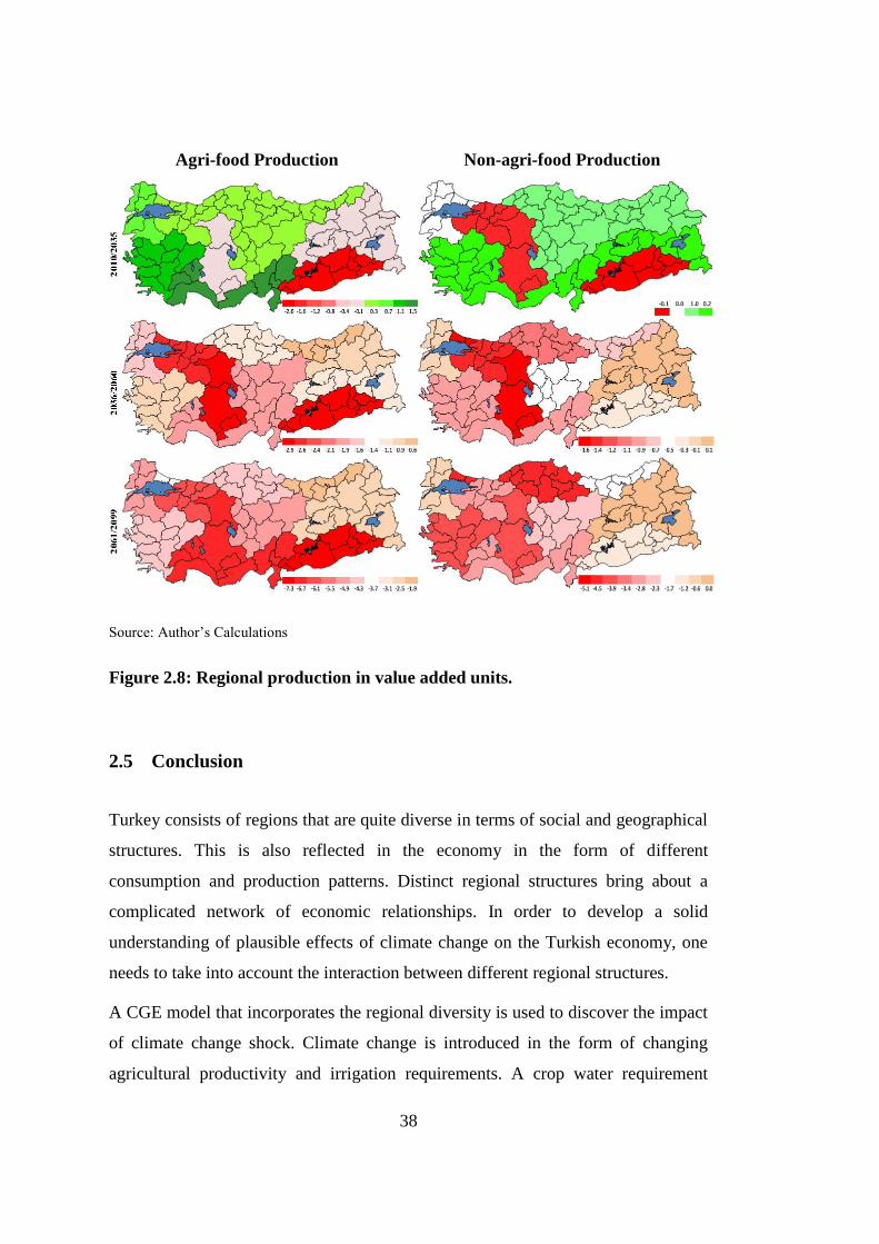
38

Agri-food Production Non-agri-food Production

Source: Author’s Calculations

Figure 2.8: Regional production in value added units.

2.5 Conclusion

Turkey consists of regions that are quite diverse in terms of social and geographical

structures. This is also reflected in the economy in the form of different

consumption and production patterns. Distinct regional structures bring about a

complicated network of economic relationships. In order to develop a solid

understanding of plausible effects of climate change on the Turkish economy, one

needs to take into account the interaction between different regional structures.

A CGE model that incorporates the regional diversity is used to discover the impact

of climate change shock. Climate change is introduced in the form of changing

agricultural productivity and irrigation requirements. A crop water requirement

39

model is used to estimate these effects for the years 2010-2099. The estimated

values of changes in the climatic conditions were obtained from a regionalized

global climate model. The results of the climate model suggest that the effects of

climate change will become significant after 2035. The average climate conditions

in the period between 2035 and 2060 will get worse, mainly due to increasing

frequency of “bad” years and higher irrigation requirements. On the other hand, the

negative impact after 2060 will be caused mainly by deteriorating average

conditions together with the increasing frequency of climatic extremes.

The effects of climate change on the economy will be witnessed through drastic

changes both in agricultural production and in the relative prices of commodities.

Production of agricultural and food commodities are severely affected by the shock,

accompanied by considerable increase in their prices. Coastal regions are affected

relatively less until 2060s, then they are significantly worse off afterwards. In all

periods, the effects on the regions which use less irrigation water are milder. This

suggests that the increase in irrigation requirements is as important as declining

yields. A similar pattern is also observed in welfare indicators. Household in the

eastern regions are affected less.

The volume of trade declines severely after 2035 and the trade balance deteriorates

in all sectors, except manufacturing. As a result, the total trade deficit decreases.

The need for agricultural and food imports become more severe and this may

contribute in giving higher priority to food security in medium and long term policy

design.

Results presented in this study are compatible with the findings of other studies at

the national or global level. The economic effects are region specific. Hence,

climate change adaptation policy needs to be region specific but should also

consider the interaction among the regions. There are welfare gains in some regions

and significant losses in others. Furthermore, the effects are also asymmetric among

economic agents. As predicted by many studies, the effects become more

significant after 2030s, especially in the form of increasing frequency of extreme

events.

40

CHAPTER 3

3. CLIMATE CHANGE, AGRICULTURE AND TRADE

LIBERALIZATION: A DYNAMIC CGE ANALYSIS FOR

TURKEY

Things should be made as simple as possible, but not simpler.

Albert Einstein

In Chapter 2, we showed that the effects of climate change would be significant for

Turkey especially after 2035. We will analyze the effects of trade liberalization in

the form of tariff elimination as an adaptation measure to climate change in this

Chapter. The model used in Chapter 2 is a static, multi-regional CGE model with

only one aggregated agricultural sector. These simplifications are required to carry

out the analysis at the regional level, but this framework may not be suitable to

analyze the effects of trade liberalization. First, Turkey’s foreign trade has a

diversified structure with respect to its trading partners. Since the rest of the world

is represented with a single aggregate trading partner, the tariffs are average tariffs

implemented on all imports. However, trade liberalization analysis requires a finer

representation of the trade structure. Secondly, an investigation of the interaction

between climate change and trade liberalization requires the introduction of time

dimension to observe the dynamics of the adjustments on the economy over time.

Thirdly protection on the agricultural imports is not homogenous across different

commodities. However, the tariff implemented on the aggregated agricultural sector

in Chapter 2 is an overall average. Hence agricultural sector needs to be represented

at a more disaggregated level, to capture the heterogeneity in protection. Lastly,

although regional details are important for scrutinizing the effects of climate

change, disaggregation of national accounts at regional level is not crucial in

41

studying the effects of trade liberalization since the commodities produced in each

region are perfect substitutes.

In this chapter, we develop a dynamic CGE model at the national level with

disaggregated agricultural sector, and diversified rest of the world accounts. Then

we simulate climate change and trade liberalization scenarios to evaluate the extent

of trade liberalization to alleviate the adverse effects of climate change. The climate

change scenario is a detailed version of the one used in Chapter 2. For the trade

liberalization scenario we simulate the elimination of the tariffs imposed by Turkey

on imports from EU27 countries.

World prices are likely to be affected by the climate change. However neither the

sign nor the magnitude of the effect is known. In order to introduce the uncertainty

about the world prices, we assume that world prices follow a normal distribution for

which the mean and the variation are affected by climate change. We assume that

under climate change, mean and variation of the distribution of world prices will

increase reflecting the worsening average conditions and increasing climate risk.

Then we use the stochastic series obtained from the simulation results to derive

conclusions about the importance of the effect of climate change on world prices.

In the following section we present the structure of the dynamic model. The

emphasis will be on the modifications done to the static model. A detailed

description of the data used to modify the SAM will follow. Then the description of

the simulated scenarios and a comprehensive discussion of the obtained results will

be provided in Section 3.3. Finally, the last section will be reserved for the

concluding remarks.

3.1 Description of the model

The model used in this study is an extended version of the CGE model presented in

Chapter 2. The model considers production activities, households, firms,

government and major trading partners of Turkey as the main economic agents and

42

attempts to model the behaviors of these agents and their interactions in a well-

established algebraic framework.

Every sector in the economy is represented with one activity that produces one

commodity using labor, capital, rainfed land, irrigated land and water together with

intermediate inputs supplied from the other sectors. The production function has a

nested structure. The first nest is a Leontief type production function between

irrigated land and water to reflect the complementarity between these two factors.

The second level nest consists of two separate production functions. The first

production function is a CES, and it transforms the water-irrigated land composite

obtained from the first level nest and other factors of production to a composite

factor. The second production function in the second nest is a Leontief production

function that transforms intermediate inputs into a composite intermediate input. In

the third level nest, the composite factor and composite intermediate input obtained

from the second level nest are introduced to another CES production function to

obtain the value added. A detailed description of the production structure can be

found in Chapter 2.

The outputs of the production activities are supplied to the domestic markets as

intermediate inputs, and final consumption goods as well as to the international

markets as exports. Production activities pay taxes to and receive subsidies from the

government.

The value added created by capital is paid to firms as income. Firms receive also

transfers from the government and the rest of the world. This income is used to pay

capital earnings to the households, institutional taxes to government and profit

transfers to the trading partners.

Households receive directly the value added created by labor, land and water as

income, while capital income is received by the firms. Households also receive

transfers from the government and the rest of the world. Household income is used

for consumption, to pay income taxes and to accumulate savings. Consumption is

43

modeled with a linear expenditure system. Households receive utility from the part

of the consumption that is above the subsistence level of consumption.

Leisure is also included in the utility function. We used the number of people who

are in the work force but who are not looking for jobs as an indicator of leisure to

overcome the calibration difficulties. People who are not in the workforce (students,

housewives, retired people etc.) are taken as a proxy for the subsistence level of

leisure. This approach can approximate the labor supply decision of the household,

but labor force participation decision is still treated exogenously in the model, since

it is impossible to endogenize the subsistence level of leisure in this framework.

However, we define a “rule of motion” for the labor force participation. Labor force

participation responses to changes in real wage. A detailed account of the

implemented utility maximization framework can be found in Chapter 2.

Saving behavior of the household is determined by the closure rule. We assume an

investment driven saving behavior at the macro level while the adjustments in

absorption are spread to the all components uniformly. Hence, the share of

investment in absorption is fixed; saving rates of the agents are uniformly scaled to

finance the investment (Löfgren et al., 2002).

There is no behavioral assumption imposed on the government. Government

collects taxes and receives transfers from the rest of the world. Government income

is used for government consumption, savings, and to make transfer payments to

domestic institutions and to the rest of the world. The share of government outlays

in total absorption is constant. We assume that government savings are flexible

while the tax rates are fixed.

Rest of the world account consists of five trading partners who supply imports and

demand exports, pay and receive transfers, and invest in Turkey. Imports follow

Armington specification while exports are modeled with a CET approach.

Accordingly, imported commodities are not perfect substitutes of domestic

alternatives and the relationship between demand for domestic and imported

commodities is managed by the substitution elasticity. The share of export supply in

44

domestic production is also managed by a constant elasticity of transformation

function. Foreign savings are always equal to the difference between value of

imports and exports to balance the current account. The share of transfers from and

to domestic institutions in their income is constant. We assume that the foreign

exchange rate for all trading partners is fixed while the foreign savings are free to

adjust.

Following Thurlow (2004), the recursive dynamic process is introduced into the

model through capital accumulation, productivity, population and labor force

growth. The amounts of the aggregate and sectoral capital in the current period are

given respectively by:

1 1t t tK K R (3.1)

, 1, ,1t A t A t Ak k r (3.2)

where denotes the amount of capital used in the activity , while is the

amount of aggregate capital stock5. is the annual growth rate of capital stock

used in activity , while is the annual growth rate of the aggregate capital

stock. The annual growth rates are calculated by

tt t

t

DR

K

(3.3)

,

, ,

,

t A

t A t A

t A

dr

K

(3.4)

5 t is the time index for all variables and parameters.

,t Ak A tK

Ar

A R

45

where is the change in real aggregate capital stock, and is the change in

real sectoral capital stock, while and denote the corresponding depreciation

rates. The change in aggregate capital is calculated as

,t

t F t

t

GFCFD

P (3.5)

where is the investment share of capital type in the total investment. Since

we have only one type of capital, is always 1. is the gross fixed capital

formation and is the price of the aggregate capital. Gross fixed capital formation

is simply the value of investment in the previous period.

1, 1, t t C t CCGFCF PQ QINV (3.6)

where is the price of commodity , is the amount of good used

for investment. The price of the aggregate capital in Equation (5) is calculated as

follows:

, ,t t C t CCP PQ B (3.7)

where are the shares of investment goods in the aggregate capital and is

calculated as

,

,

,

t C

t C

t CC

QINVB

QINV (3.8)

Lastly the sectoral capital stock is calculated by

, ,t A t A tD D (3.9)

tD,t Ad

t t

,F t F

t tGFCF

tP

,t CPQ C,t CQINV C

,t cB

46

where is the investment share of the capital stock of activity in an aggregate

capital stock. is calculated as follows:

, ,

, 2

,

1 1t A t A

t A

t A tA

K W

K W

(3.10)

where is an exogenous constant that determines the mobility of capital across

sectors, is the price of capital in sector . is the average price of capital

and is calculated by

,

,

,

t A

t t AAt AA

KW W

K

(3.11)

In other words, shows the share of investment in sector adjusted for the

differences in the price of capital. When the price of capital increases in a sector, a

relatively higher portion of the gross fixed capital formation is devoted to that

sector.

Productivity growth is introduced as an exogenous increase in the shift parameter of

the top level CES production function, .

, 1, ,1t A t A t A (3.12)

where is the total factor productivity growth.

Population growth causes changes in two parameters in the model, which also need

to be considered: an increase in the subsistence level of consumption and an

increase in the labor force. Subsistence level consumption growth is introduced as

an exogenous shock to the subsistence level consumption parameter, .

,t A A

,t A

2

,t AW AtW

A A

,t A

,t A

t

47

1 1t t t (3.13)

where is the population growth rate. Growth in the labor force is also introduced

as an exogenous change in the number of people participating in the labor force,

denoted by .

1 1t t tL L (3.14)

where is the labor force growth. It is necessary to distinguish between the labor

force growth and population growth, since the former is generally lower than the

latter. Note that the increase in labor force does not necessarily imply increasing

labor force participation since labor force participation is determined by real wage.

3.2 Description of Data

The social accounting matrix (SAM) used in this Chapter involves making three

modifications to the SAM used in Chapter 2. First, the SAM used in Chapter 2 is

aggregated to the national level. Secondly, the agricultural sector of the SAM used

in Chapter 2 is disaggregated into 13 sub-activities: wheat, maize, rice, other

cereals, oilseeds, sugar beet, other field crops, fruits, vegetables, dairy, meat,

livestock and other agricultural production. Thirdly, rest of the world account is

disaggregated into five trading partners who supply imports and demand exports,

make and receive transfers, and invest in Turkey. Non-agricultural sectors are kept

intact. There are 4 manufacturing activities (food, textiles, energy and other

manufacturing production) and 2 services (private and public services).

The disaggregation of the agricultural sector is accomplished using the 2008

production statistics (TurkSTAT, 2012a). We assumed that input-output (I/O)

coefficients of all disaggregated activities are the same as the aggregate agriculture

(TurkSTAT, 2012b). We then introduced some adjustments in the I/O table. Crop

production activities use only their own commodities as intermediate inputs and no

t

tL

t

48

other crop products. Milk and meat production activities are linked only with

livestock production activity which mainly consists of livestock raising. Livestock

activity uses wheat, maize and sugar beet as feed. Agricultural activities do not use

any textiles or public services commodities. To balance the I/O table for the

agricultural activities, we increased the intermediate input use of food production

activity from the agricultural activities. Hence a significant part of the intermediate

input supply of agricultural activities is used by food production. Textiles

production activities use inputs only from other cereals and other field crops. The

energy sector receives input from sugar beet production to reflect the small amount

of ethanol production in Turkey. Minor adjustments are done to balance the other

sectors in the I/O table. The value added of land is calculated from irrigated and

rainfed land rent data reported by G&G Consulting et al. (2005). The share of

irrigated land in the total cultivated land is obtained from the agricultural master

plans of 81 provinces (Ministry of Food Agriculture and Livestock, 2012). These

shares are then used to find the total irrigated land at the national level. We assume

that the share of irrigated and rainfed land is the same across different crops, since

there is no data at the crop level for the use of irrigated land. However we used

priori information for the use of irrigated and rainfed land by specific crops. For

example, the production of rice and vegetable requires irrigated land. The value

added for water is calculated from the rental difference between the rainfed and

irrigated land at 12 NUTS-1 level from G&G Consulting et al. (2005) and

aggregated to the national level by using irrigated land data.

Agricultural subsidies are introduced to the national SAM using the OECD data as

negative activity taxes. Then capital value added account is adjusted accordingly.

The results are presented in Table 3.1. According to OECD (2013) the highly

supported activities are livestock, other field crops, wheat and dairy. Rice and

vegetables do not receive any subsidies while support for meat, fruits and other

cereals are quite low.

49

Table 3.1: Subsidies on agricultural activities (Thousand TL)

Activity Subsidy Activity Subsidy

Wheat 673,138 Fruits 3,775

Maize 71,414 Vegetables 0

Rice 0 Dairy 310,252

Other Cereals 6,163 Meat 1,210

Oil Seeds 114,583 Livestock 853,277

Sugar Beet 16,722 Other Agriculture 49,027

Other field Crops 682,500

Source: Authors’ calculation from OECD (2011)

Households do not directly consume wheat, maize, other cereals, oilseeds, sugar

beet, other field crops, livestock and other agricultural products. The outputs of

these activities are used as intermediate inputs, mostly by the food production

activity. Households, however, directly consume rice, fruits, vegetables and dairy

products. We assume that ‘government’ does not consume any agricultural

products. The resulting consumption pattern is given in Figure 3.1 with ‘private

services for the households’ being the most important consumption item with a 45

percent share. Agri-food products constitute 24 percent of the total consumption; 17

percent of which is made up of processed food.

The ROW account is disaggregated into 5 trading partners: EU27, MENA, North

America, Other Europe, and the Rest of the World. Imports are distributed across

trading partners according to foreign trade statistics (TurkSTAT, 2012c). Minor

adjustments in saving-investment account were necessary to balance the

discrepancy in the trade accounts.

50

Source: Author’s calculations from the SAM

Figure 3.1: Consumption pattern of households

Tariffs are recalculated according to the GTAP data. We made minor adjustments in

the SAM since the reported amount of tariff revenue is lower than the revenue

obtained when the GTAP tariff rates are implemented. The increase in tariff

revenue is added to the government account while the same amount is discounted

from the supply of commodities. The decline in supply is then balanced by reducing

the capital value added and hence the capital income of firms is reduced. Transfers

from the government to firms are then increased by the same amount to keep

household income intact. Changes in capital and government transfers to firms are

small relative to the initial levels of these accounts.

The tariff rates used in the model are given in Table 3.2. Although the Turkish

protection against EU imports is low at the average, dairy products, meat and fruit

imports are heavily taxed. High protection against the other regions is likely to

favor EU products in case of trade liberalization. The main competitor of the EU27

countries in the Turkish imports market is ‘other European countries’. According to

the baseline data, Turkey’s imports of cereals from other European countries are

higher than the amount of imports of these commodities from EU27.

51

Table 3.2: Tariff rates according to trading partners (percent) EU27 MENA North America Other Europe Rest of the World

Wheat 28.5 43.3 42.9

Maize 125.1 121.2

Rice 32.1 0 32.1 31.6

Other Cereals 92.3 125.1 97.9 121.2

Oil Seeds 1.2 4.8 4.8 8.4

Sugar Beet

Other field Crops 9.3 12.2 15.6

Fruits 39.1 24.5 35.4 59.5

Vegetables 24.5 59.5

Dairy 101.8 116.4 122.8 118.5

Meat 83.6 22.1 7 102.6

Livestock 2.0 4.9 5.3

Other Agriculture 2.3 7.1 0.1 1.9

Other Manufacturing 0 3.9 2.7 1.8

Food Production 12.3 16.9 18.9 21.2

Textiles 0 6.5 5.1

Energy 0 0 0.3

Services 0

Source: Authors’ calculation from (Narayanan et al., 2008).

Foreign savings and transfers from firms to trading partner accounts are distributed

across trading partners according to the foreign direct investment data reported in

the General Directorate of Foreign Capital (2009). Transfers from trading partners

to households (i.e. mainly workers’ remittances) are distributed according to the

data reported by the World Bank (2012). Transfers from trading partners to firms

are distributed according to the Turkish foreign direct investment in other countries

as reported by OECD (2012). This means that that the money transferred from

abroad to the firms are mainly profits of firms from abroad and they are

proportional to the investment made abroad. The results are given in Table 3.3.

The remaining accounts are obtained by aggregating the SAM developed in Chapter

2 over the regions. The compilation methods and assumptions used there remained

unchanged.

52

Table 3.3: Foreign savings and transfers (TL million)

EU27 MENA

North America

Other Europe

Rest of the World

Tra

nsfe

rs

from Firms to ROW 10,136 536 1,021 1,072

from Government to ROW 19,151 63,195

from ROW to Households 1,317 140 189 130 78

from ROW to Firms 2,979 4,434 461 1,113

from ROW to Government 16,907 5,381 53,902

Foreign Savings 46,745 2,472 4,709 4,945

Source: Authors’ own calculation

3.3 Trade Liberalization between EU and Turkey

Trade relationship between Turkey and the EU has been shaped mainly by the

Custom Union (CU) Decision of 1996. The benefits and costs of the agreement

have been the topic of many studies in the literature since then. Starting from the

year 2000, a significant effort has been also devoted to understand the possible

economic effects of liberalization of agricultural trade between EU and Turkey.

Studies in the literature generally focus on full accession of Turkey to the EU or

extending CU decision to agricultural products. So far, the results are ambiguous,

but some general trends can be identified.

The foremost addressed question in the literature regarding the full trade

liberalization between EU and Turkey focuses on the sign and size of possible

welfare effects. Most of the studies reports around 0.5 percent welfare gain or GDP

increase under various agricultural trade liberalization scenarios (Eruygur, 2006;

Harrison et al., 1997; Lejour et al., 2004; Mercenier et al., 1997; Özer et al., 2009).

On the other hand, a deeper integration with the EU is reported to provide higher

levels of gain for Turkey. Such actions as: improving EU market access (Harrison et

al., 1997), the abolition of nontariff barriers by Turkey (Mercenier et al., 1997;

Zahariadis, 2002), the inclusion of Turkey in the CAP support system (Eruygur,

2006; Nowak-Lehmann et al., 2007), creating a sustainable competitive

environment (Bayar et al., 2000), maintaining a flexible labor market (De Santis,

53

2000), improvement of the national institutions and free movement of labor (Lejour

et al., 2004), taking into account the scale economies (Sulamaa et al., 2006), timing

of liberalization (Acar et al., 2007), harmonization with the EU’s health and safety

standards (Oskam et al., 2004) are all reported to increase the gains from trade

liberalization for Turkey. Depending on the modeling structure and assumptions

about the way trade liberalization is implemented, it can be stated that an extension

of CU to agricultural sector would result in a welfare gain between 0.5 to 1.5

percent of GDP annually. However, only a few studies report either insignificant

total welfare effects (Augier & Gasiorek, 2003; Çağatay, Saunders, & Amor, 2001;

Çakmak & Kasnakoğlu, 2003; Grethe, 2004) or even welfare losses (Bekmez, 2002)

for Turkey.

The winners and the losers from agricultural trade liberalization are also heavily

investigated. The results depend on the scale and structure of the models. Partial

equilibrium models give a clear answer for the distribution of welfare gain from

trade liberalization across producers and consumers. Producers are generally

reported to be losing, while consumers gain (Çakmak & Kasnakoğlu, 2003; Grethe,

2004; Oskam et al., 2004). The main reason for this is the declining producer prices

as a result of liberalization. However, this effect is not uniform across all producers

(Oskam et al., 2004). Crop producers are generally worse off (Fellmann et al., 2011)

while the effect on livestock producers’ welfare is ambiguous. Çakmak &

Kasnakoğlu (2003), Grethe (2004) and Eruygur (2006) report negative effects while

Fellmann et al. (2011) and Leeuwen et al. (2011) report positive effects. As well,

consumers’ gain is not uniform. De Santis (2000) reports that urban population

would be better off, while rural population is likely to be worse off under CU,

although the effect on income distribution would be negligible.

Studies based on global or multiregional CGE models provide country or region

specific results. The global effect of agricultural trade liberalization between Turkey

and EU is found to be negligible (Sulamaa et al., 2006). Change in EU welfare is

insignificant whether it is positive (Alessandri, 2000; Augier et al., 2003;

Zahariadis, 2002) or negative (Acar et al., 2007; Adam et al., 2008; Alessandri,

54

2000; Francois et al., 2005). These effects are also not uniform within the EU.

Given the fact that Turkey’s main competitors for EU market access are the

Southern European countries, Southern European countries are more likely to lose

while northern European countries win (Nowak-Lehmann et al., 2007; Sulamaa et

al., 2006).

The findings about the effects on trade are ambiguous. There is no doubt that the

overall effect on volume of trade between Turkey and EU will increase (Bekmez,

2002; De Santis, 2000; Lejour et al., 2004). In some cases this is accompanied with

a significant trade diversion (De Santis, 2000). Some studies report that Turkey will

become a net importer of crops (Çağatay et al., 2001), while others state that crop

exports will increase more than the imports (Çakmak & Kasnakoğlu, 2003; Grethe,

2004; Özer & Özçelik, 2009); others assert that Turkey will be net importer of

livestock products (Grethe, 2004). Almost all find that fruits and vegetable exports

will increase (Çakmak, 2007; Eruygur, 2006; Nowak-Lehmann et al., 2007).

Impacts of trade liberalization under climate change have not been subjected to any

analytical studies for Turkey. However, the issue of interaction between trade

liberalization and climate change has been addressed at the global scale. The main

argument in the literature is that trade liberalization can alleviate the negative

effects of climate change by boosting international trade. Trade liberalization is

reported to have welfare improving effects (Calzadilla et al., 2011; Chen et al.,

2012; Laborde, 2011; Reilly et al., 1993). However these effects are generally weak

and won’t compensate for the adverse effects of climate change (Randhir & Hertel,

2000; Reilly & Hohmann, 1993). Welfare gains from trade liberalization are

dependent on the elimination of production and export subsidies (Randhir et al.,

2000). The effects are not uniform and depend on the geographic location

(Calzadilla et al., 2010; Reilly et al., 1993) and the degree of regional vulnerability

to climate change (Reilly et al., 1993). Poor people are expected to be affected more

from the changes (Laborde, 2011).

55

To sum up, trade liberalization is expected to increase the welfare of Turkey,

especially through its effects on consumers. However, the findings in the literature

are quite diverse and vary based on the data and method of analysis, and exclude the

effects of climate change. Most of the studies rely on quite old databases such as the

GTAP database with the base year being 1997, long before CU became fully

functional. Almost all studies employ static models which ignore the dynamic

aspects of the problem. Almost all CGE models lack a detailed disaggregation of

agriculture while partial equilibrium models ignore the feedback mechanisms.

In this chapter we try to fill the gap in the literature with a detailed and enhanced

modeling framework. The welfare effects of trade liberalization and its reflection in

production, consumption and food security will be at the center of our analysis. We

will also explore the relationship between climate change and trade liberalization to

see if trade liberalization can alleviate the adverse effects of the climate change. We

will address whether unilateral trade liberalization can be considered as a policy

alternative to help climate change adaptation efforts of Turkey.

3.3.1 Scenario Design

To simulate the effects of trade liberalization between EU and Turkey under climate

change, we run three scenarios over the period 2008-2099. First, we run a baseline

scenario that mimics the growth path of the Turkish economy for the period 2008-

2099. The results of the baseline scenario are used for benchmarking the other

scenarios. Climate change effects on yields and irrigation requirements are then

incorporated on top of the assumptions made for the baseline in the second scenario.

Lastly, we introduce unilateral tariff elimination by Turkey against the EU imports

as a policy response to climate change effects. Climate change and tariff elimination

scenarios are run under 52 different changes in the world prices for each year. The

series for world price changes are calculated using the Gaussian-Quadrature method

from the historical world price series for each commodity.

56

We start this section with the description of the scenarios. Then the simulation

results are discussed. More emphasis will be given on the results of trade

liberalization scenario by benchmarking them against the results of the climate

change scenario.

Baseline Scenario

The baseline is the “business as usual” scenario where we try to mimic the historical

growth rate of the economy over the period 2008 and 2099. In other words, the

model is calibrated to yield an average GDP growth rate of 3.5 percent, which is the

average growth rate of GDP between 1950 and 2008 (TurkSTAT, 2010b). The

annual population growth is assumed to be 0.9 percent. The subsistence

consumption levels are automatically updated to reflect the increase in population.

Labor force endogenously adjusts to the population growth by taking into account

the change in real wages. The resulting change in labor supply is given in Figure

C.5.

We assume that the annual total factor productivity (TFP) growth is 0.8 percent in

agriculture, 1.06 percent in industry and 0.4 percent in services. We use the yield

projections for wheat presented in Bruinsma (2003) and reported in Kavallari, Rau,

& Rutten (2013). We assume that TFP growth in services is half of the increase in

agricultural activities, while the industrial TFP growth is 2.65 times the TFP growth

in services. Capital growth is endogenous in the model. The growth in capital stock

is determined by the dynamics of the model. We assume that the default

capital/output ratio is 4.2 6 and the depreciation rate is 3 percent. We do not change

the world prices in the baseline since we assume that world prices are changing due

climate change.

6 We calculated 4.2 as capital/output ratio from the data published by the Ministry of Development

(2012).

57

Climate Change Scenario

This scenario introduces climate change effects to the baseline. These effects are in

the form of yield and irrigation requirement changes. They are obtained from the

crop water requirement model described in Annex A for all crops at the national

level. We use a 5-year moving average for the yield change since there are

significant outliers for a few highly irrigated crops. This reduces the extreme events

caused by frequent harvest failures foreseen by the crop model. However, deviation

from the base year is still significant (Figure 3.2) and the story line for the climate

change effects does not change. Yields are generally increasing between 2008 and

2035; they start to decline between 2036 and 2060. In the last period, 2061-2099,

the decline in yields becomes substantial. Irrigated water requirement oscillates

significantly throughout the all periods.

Yields of fruits and cereals are not affected much while maize and oilseeds are the

most affected crops. The impact is reversed in the case of irrigation water

requirements. Effects on wheat, vegetables and other field crops are significant both

in terms of yields and irrigation requirements. All crops more or less follow the

pattern in Figure 3.2. In the first period the change in average yields is rather small

and even positive for some crops. Yields of all crops start to decline in the second

period, but the magnitude of the average decline is not more than 10 percent.

However, the decline becomes prominent in the last period, especially for maize

and oilseeds. Yield and irrigation water requirements at the activity level are given

in the Appendix Figure C.1. Descriptive statistics for the introduced shocks

according to the periods can be found in appendix Table C.1.

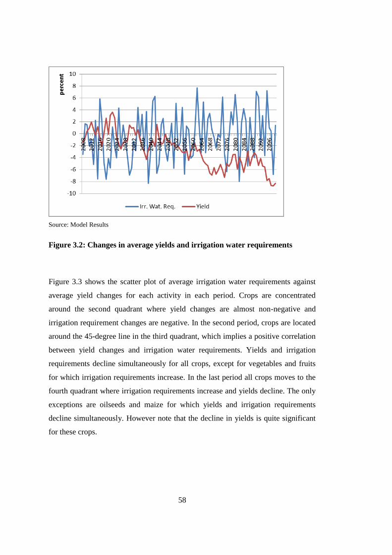
58

Source: Model Results

Figure 3.2: Changes in average yields and irrigation water requirements

Figure 3.3 shows the scatter plot of average irrigation water requirements against

average yield changes for each activity in each period. Crops are concentrated

around the second quadrant where yield changes are almost non-negative and

irrigation requirement changes are negative. In the second period, crops are located

around the 45-degree line in the third quadrant, which implies a positive correlation

between yield changes and irrigation water requirements. Yields and irrigation

requirements decline simultaneously for all crops, except for vegetables and fruits

for which irrigation requirements increase. In the last period all crops moves to the

fourth quadrant where irrigation requirements increase and yields decline. The only

exceptions are oilseeds and maize for which yields and irrigation requirements

decline simultaneously. However note that the decline in yields is quite significant

for these crops.

59

Source: Model Results

Figure 3.3: Yield and irrigation water requirement changes in periods

Climate change is a global phenomenon and hence it is likely to affect world prices

of agricultural commodities significantly. However, it is not possible to capture this

effect with a small single country model where world prices are assumed to be

exogenously determined. Many studies in the literature ignore this effect. We

incorporate the effects of climate change on world prices as exogenous shocks. In

other words, we assume that climate change does not only affect the yields and

irrigation requirements but also the world prices.

There are various studies in the literature that attempts to quantify climate-induced

changes on world prices by using global CGE models. These studies generally

report significant changes in world prices of major staples. However we cannot

incorporate these findings in our simulations since their assumptions about the

climate change are generally different from that of ours. Further these studies are

generally static exercises and report world prices only for a specific year. Lastly, the

reported world price changes are generally inconsistent. Hence instead of taking

world price changes from other studies in the literature we use Gaussian Quadrature

method to generate different world price series.

60

Gaussian quadrature is an approximation method for numerical integration.

Weighted sum of function values at specific points in the domain of the function are

used to approximate the value of the function (DeVuyst and Preckel, 1997).

Gaussian quadrature method gives the weights and nodes in the following

approximation:

1

n

i i

i

f x dx f x w

(3.15)

where is a continuous function, is the vector of independent variables,

is the vector of nodes selected in the domain of the integral, are weights assigned

to the value of the function at corresponding nodes and are called quadratures, is

the minimum number of the nodes required for a good approximation. There are

various formulas in the literature to calculate the weights and nodes efficiently.

Strauds method is used widely in the CGE literature (Arndt, 1996). Strauds method

solves the following equation system to find nodes and weights.

1 1 1

0,1,2....,m m

bM MNl l

m m

i i i

i m ma

w x x f x dx s d

such that 1

m

j

j

l d

(3.16)

for all combinations of nonnegative integers, . is known as the order of the

quadrature. Many formulas for different orders and arbitrary dimensions of

quadratures are developed in the literature. Most frequently used formulas are

derived by Stroud (1957) and Liu (1997) for order 3 quadratures (Arndt, 1996),

which are exact for orders smaller than 3 (Preckel et al., 2011). If is the kth

quadrature point with the elements such that and if

where is the greatest integer smaller than , then it can

be shown that

2 1 2

2 1 2 12 cos 2 sinr r

r k r k

n n

(3.17)

f x x ix

iw

n

ml d

k

,1 ,2 ,n, ,...,k k k 1,2,...,k n

1,2,..., 2r n 2n 2n

61

yields the elements of the which is the kth

quadrature. If n is an odd number

then , 1k

k n . In this case weights are equal and sum up to 1:

1

2kw

n (3.18)

Gaussian quadrature method is used for stochastic sensitivity analysis in the CGE

literature and is shown to be quite efficient in capturing the uncertainty in the

parameter values (Arndt, 1996; DeVuyst and Preckel, 1997). Stochastic sensitivity

analysis assumes that model parameters are stochastic variables following a

distribution function. Hence the values used in the model are just one point drawn

from this distribution. In this case model results are also stochastic. If we consider

the CGE model as a function that relates the pre-simulation and post simulation

values of the variables in the model, then the expected value and variation of the

post-simulation values of the variables can be approximated by using Gaussian

quadrature approach. In this way one can select a limited number of parameter sets

and weights and run the model for these parameter sets. Then the stochastic

properties of the model results can be derived from the output of these runs. A high

variation in the values of key model variables would mean that model is sensitive to

the relevant parameters.

To conduct a sensitivity analysis with respect to a symmetrically distributed random

variable vector that consists of elements with mean and variance

covariance matrix , the desired quadrature is given by

D (3.19)

where D is a diagonal matrix obtained by Cholesky factorization:

'LDL (3.20)

Then is obtained by transforming the quadrature in equation (3.17) by

k

x 1 2, ,..., nx x x

62

L (3.21)

If is diagonal then

(3.22)

Preckel et al. (2011) propose an algorithm to extend the quadratures suggested by

Straoud. They propose to use two copies of the Straoud quadratures: stretching one

and shrinking the other to achieve the desired broadening of the sample while

keeping the mean intact and redistributing the weights (or probabilities) so that the

variance is maintained. Hence they introduce an expansion factor, denoted by , a

contraction factor, denoted by , and a probability allocation factor, denoted by p.

The resulting quadrature is

1 1, , 1 ,

n ni i i i

i ipw x p w x

(3.23)

Preckel et al. (2011) show that once the expansion factor, , is chosen, the

parameters and are given by

2

4 2 2

1

2 1q

(3.24)

We follow this approach to capture the variation in the model’s results due to the

world prices. Accordingly, we assume that percentage change in real world price of

each agricultural commodity follows a symmetric distribution. The mean of the

distribution is assumed to be zero for all commodities in the base period. Then we

assume that the mean of the distribution will increase by one, two and three

standard deviations in the first, second and last period respectively. We further

increase the variation in the percentage change of the world prices (i.e. diagonal

elements of the variance covariance matrix) by one percent in each period. Hence in

each period we assume that mean of the distribution of percentage change in world

prices are increasing together with the variation in the prices. These assumptions are

p

63

compatible with the recent studies in the literature (Hertel and Rosch, 2010;

Valenzuela and Anderson, 2011a and 2011b; Diffenbough et al., 2012; Calzadilla et

al., 2013).

Changes in the world prices of different commodities are not independent from each

other. This stems from two facts. Firstly, different agricultural commodities are

substitutes to some extent. Hence their prices are linked to each other. Secondly,

price changes are linked to production, and production of all commodities is

dependent on the same climate conditions. For example, if the price of one

commodity is rising due to drought, other crops will be affected from the drought as

well and their prices will also rise. To take this correlation into account we form the

variance covariance matrix by using the historical correlation between the annual

price changes of the commodities. We eliminate small correlations to avoid

problems in Cholesky decomposition. We also assume that correlation among the

percentage change of world prices of different commodities remains constant over

time.

Table 3.4 shows the expected values and standard deviations of the world price

shocks calculated by Gaussian quadrature method for all commodities over the

three periods. Our assumptions yield world price changes that are consistent with

the climate change patterns. The average percentage change increase over time is as

expected. The highest increases occur in the world price of rice, wheat, oilseeds and

other field crops. Variations for these crops are also high. The lowest increases, on

the other hand, occur in vegetables, meat and other agricultural crops.

We run the climate change simulations by shocking the shift parameter of the top

level CES production function with the yield changes, the coefficient of water in

irrigated land – water nest with irrigation water requirements and the world prices

with the world price change series generated by Gaussian quadrature. Hence, we

run 48 simulations each with a different world price assumption. Therefore the

results for the levels of the variables show the expected values. We also report the

standard deviations when it is appropriate.

64

Table 3.4: Mean and standard deviation of the world price shocks

Period 1 Period 2 Period 3

Exp. Val. Std. Dev. Exp. Val. Std. Dev. Exp. Val. Std. Dev.

Wheat 1.01 1.46 2.01 1.46 3.01 1.46

Maize 0.62 0.76 1.62 0.76 2.62 0.76

Rice 1.27 1.67 2.27 1.67 3.27 1.67

Oth. Cereals 0.99 0.62 1.99 0.62 2.99 0.62

Oilseeds 1.72 0.95 2.72 0.95 3.72 0.95

Oth. Fld. Crp. 3.06 1.10 4.06 1.10 5.06 1.10

Fruit -0.18 0.57 0.82 0.57 1.82 0.57

Vegetable 0.50 0.26 1.50 0.26 2.50 0.26

Milk -0.12 0.85 0.88 0.85 1.88 0.85

Meat 5.55 0.41 6.55 0.41 7.55 0.41

Livestock 4.15 0.85 5.15 0.85 6.15 0.85

Other Agriculture 3.63 0.39 4.63 0.39 5.63 0.39

Note: Mean and standard deviation are first and second moments of distribution, respectively

Source: Author's calculations

Trade Liberalization Scenario

Under the trade liberalization scenario we assume that all tariffs implemented by

Turkey on EU imports are unilaterally eliminated on top of the climate change

scenario. This scenario is called “Tariff Elimination scenario (TRF)”, and

eliminated tariffs are given in Table 3.5. Protection is generally high in agricultural

commodities. The share of agricultural imports in the total imports from EU is low

with a value of less than two percent. On the other hand, EU’s share in agricultural

imports of Turkey is significant varying between 20 to 45 percent. Although

agriculture is a minor item in imports from EU, EU is still the most important

trading partner of Turkey. Hence trade liberalization with EU is likely to have a

significant direct impact on Turkish agriculture while the impact on the rest of the

economy will be through the backward and forwards linkages of agriculture with

the other sectors.

65

Table 3.5: Tariffs imposed by Turkey (percent)

Tariff Rate Share of EU in total imports of

commodity

Share of commodity in total imports

from EU

Wheat 28.5 25.2 0.36

Maize 0 0.0 0.00

Rice 32.1 19.8 0.03

Cereals 92.3 21.9 0.02

Oil Seeds 1.2 28.6 0.39

Sugar Beet 0 0.0 0.00

Field Crops 9.3 30.4 0.03

Fruits 39.1 9.6 0.03

Vegetables 0 0.0 0.00

Dairy 101.8 39.6 0.05

Meat 83.6 12.0 0.00

Livestock 2 35.8 0.02

Oth. Agriculture 2.3 45.9 0.09

Manufacturing 0 52.3 82.69

Food 12.3 24.0 0.85

Textiles 0 28.6 2.19

Energy 0 8.0 0.00

Services 0 52.3 13.24

Source: Authors’ calculation from (Narayanan et al., 2008).

3.3.2 Simulation Results

In this section we present the main conclusions from the simulation results and

explore the main drivers of change in order to derive policy implications. We will

present the results relative to the changes in the baseline scenario. The main results

of baseline scenario are given in Appendix A.2.3. In this section, we will first give

an overview of macro results of the two scenarios. Then we will focus on the effects

of trade liberalization by presenting them relative to the results of climate change

scenario.

66

3.3.2.1 Macro Results and Welfare Effects

The results obtained are largely consistent with what have been suggested in the

literature and provide important insights about the main drivers of the effects of

climate change. Figure 3.4 shows the expected value of the equivalent variation7

(EV), which is an indicator of welfare gains for the households. Change in EV is

between -3.3 percent and +1.3 percent of the initial household consumption for

climate change scenario and -2.8 percent and 1.63 percent for the trade

liberalization scenario.

EV is higher under trade liberalization compared to the climate change scenario.

However, the trade liberalization is far from alleviating the negative effects of

climate change. In the last period, 2060-2099, the EV is always negative under both

scenarios. Though, the difference between the climate change and the trade

liberalization scenarios increases as the effects of climate change worsen. This

suggests that the welfare improving effects of trade liberalization are enhanced

when the effects of climate change are worsened. As agricultural production

becomes less productive as a result of the climate change, welfare improving effects

of trade liberalization are amplified. This is mainly due to the fact that trade

liberalization allows economic agents to substitute domestic and imported

commodities more freely. Consumers can consume more imported commodities as

a substitute to the domestic products which become relatively scarce under climate

change. Producers can also substitute domestic intermediate inputs with imported

inputs to compensate the decline in the productivity of land. Consequently, the more

agriculture is affected from climate change the higher is the welfare improving

effect of trade liberalization.

7 More formally, EV shows the minimum payment that the consumer would require for foregoing the

welfare gains under the relevant scenario (Sadoulet and Janvry, 1995).

67

Source: Model Results

Figure 3.4: Expected value of equivalent variation

The change in GDP is generally small until the 2060s (Figure 3.5). Changes in

tariffs may not be fully reflected in the production side of the economy up to this

period. The impacts of tariff elimination are generally absorbed by the substitution

mechanisms in trade, consumption and production. GDP starts to decline after 2035

but the decline is significant only after 2060s. This is consistent with what is

generally reported in the literature. The trends are similar to those we noted in

Chapter 2. Welfare and other macro indicators follow the same path: they get better

off in the first period (2008-2035), start to decline in the second period (2035-2060)

and worsen in the last period (2060-2099). Thus, Turkey is likely to have time to

take necessary measures for adaptation before climate change has significant

impacts at economy level. Furthermore ignoring the probable adverse effects of the

climate change in the second and the last period can have devastating effects and

significant costs for all economic agents.

68

Source: Model Results

Figure 3.5: Real GDP over time (percentage deviation from baseline)

Figure 3.6 shows the evolution of the standard deviation of the GDP and the EV

over time. Since we use the same world price shocks in both climate change and

trade liberalization scenarios standard deviations in both simulations are very

similar. Hence for the sake of clarity we will present only the standard deviations

for the trade liberalization scenario.

The standard deviation of EV increases in the first two periods and it stabilizes and

follows a horizontal trend after 2060s. On the other hand, although the standard

deviation of the GDP starts at a low level compared to the standard deviation of EV,

it increases throughout the simulation period. Thus we can conclude that although

changes in world prices do not cause any further changes in the variation for

household welfare in the last period, their impact on the variation of the GDP

persists. This implies that changing world prices affect both the consumption and

production sides in the first period and only the production side in the last period.

69

Source: Model Results

Figure 3.6: Standard deviation of EV and GDP levels over time

Figure 3.7 shows the decomposition of the changes in GDP under the climate

change scenario. The most important drivers of the change in the GDP are private

consumption, imports and exports. Government consumption contributes very little

to the changes in the GDP and therefore its activity on change will not be reflected

in this figure. Changes in fixed investments are however included, and in spite of

their minimal influence at the start, their contribution becomes more significant in

the last period.

The contribution of the changes in private consumption to the changes in GDP

moves generally in opposite direction compared to those in trade. This is valid

throughout the whole simulation period. In the first period, trade contributes

negatively to the changes in GDP, implying a decreasing value of exports and an

increasing value of imports in the first period. The decline in total exports is caused

mainly by a decline in exports to the regions other than EU27.

70

Source: Model Results

Figure 3.7: Contribution of the GDP components on the GDP change under

climate change scenario (percentage deviation from the baseline)

In the second and third period, however, the effects are reversed. In the second

period, the positive contribution of imports and exports are able to compensate the

negative contribution from consumption. However, in the third period the combined

effect of consumption and fixed investments has a stronger influence than the

combined effect of imports and exports, and as a result GDP declines significantly.

In the second and third periods the effects of consumption and trade are almost

symmetrical around the horizontal axis since increasing exports and decreasing

imports due to increasing world prices put a significant pressure on consumption.

Thus consumption adjusts to handle the change in the world prices.

The contributions of the components of GDP to the changes in the overall GDP

under the trade liberalization scenario are presented in Figure 3.8. Private

consumption and fixed investments have positive impact on GDP (i.e. less negative,

under trade liberalization), while exports’ contribution is almost the same between

the two scenarios. However, positive contribution of imports decreases under the

trade liberalization scenario. That is, as import prices decline the imports are

71

substituted with domestic commodities and this increases the consumption. The

changes are weak, as they are not likely to reverse the sign of the GDP change.

Hence, trade liberalization only weakly alleviates the effects of climate change in

terms of GDP growth. Note that the difference gets higher over time. Hence, the

benefits of trade liberalization increase as climate shocks get significant.

Source: Model Results

Figure 3.8: Contribution of GDP components to the GDP change under trade

liberalization scenario (percentage deviation from climate change scenario)

Figure 3.9 and Figure 3.10 show the sectoral decomposition of the change in

imports and exports under climate change scenario with respect to the baseline.

Contribution of services to the change in imports and exports is small compared to

the agri-food and manufacturing. The main driver of the change in imports is

manufacturing, especially in the first period. The contribution of manufacturing is

generally positive in the first period while it deteriorates significantly in the second

and third periods.

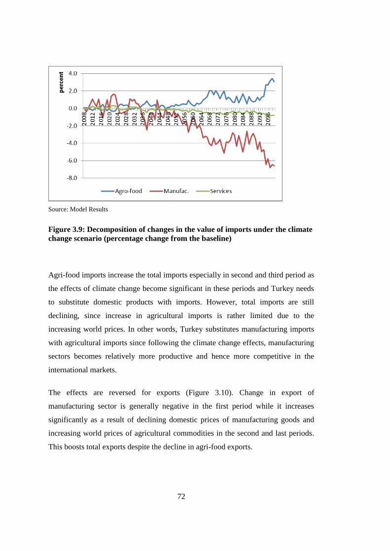
72

Source: Model Results

Figure 3.9: Decomposition of changes in the value of imports under the climate

change scenario (percentage change from the baseline)

Agri-food imports increase the total imports especially in second and third period as

the effects of climate change become significant in these periods and Turkey needs

to substitute domestic products with imports. However, total imports are still

declining, since increase in agricultural imports is rather limited due to the

increasing world prices. In other words, Turkey substitutes manufacturing imports

with agricultural imports since following the climate change effects, manufacturing

sectors becomes relatively more productive and hence more competitive in the

international markets.

The effects are reversed for exports (Figure 3.10). Change in export of

manufacturing sector is generally negative in the first period while it increases

significantly as a result of declining domestic prices of manufacturing goods and

increasing world prices of agricultural commodities in the second and last periods.

This boosts total exports despite the decline in agri-food exports.

73

Source: Model Results

Figure 3.10: Decomposition of change in exports under climate change

scenario (percentage change from baseline)

Trade liberalization does not change the contribution of sectors to trade

significantly (Figure 3.11 and Figure 3.12). However, the contribution of

manufacturing sector to the change in total imports starts with two percent and

climbs up to eight percent. This implies that the negative contribution of

manufacturing sector to the total imports decreases by 10 percent throughout the

whole period. This points out the importance of the manufacturing sector for the

rest of the economy to adjust the adverse effects of the climate change.

The contribution of manufacturing sector to the change in total exports decreases

under trade liberalization and this effect does not follow a consistent path. The

effects of trade liberalization on the contribution of agri-food imports are stable

around 0.3 percent while the effect on exports is negligible.

74

Source: Model Results

Figure 3.11: Decomposition of change in value of imports under trade

liberalization (percentage change from the climate change scenario)

To sum up, effects of climate change become significant after 2035 with declining

welfare and GDP. Imports are reduced substantially while there is a boost in

exports, mainly due to manufacturing sector. Trade liberalization wirth EU in

agricultural commodities is likely to have a limited overall effect to alleviate the

adverse effects of climate change.

Welfare gains are positive but not significant enough to change the sign of the

overall effects. On the production side, the total value added does not change much

from the climate change scenario implying a limited feedback effect. The main

drivers of change on the GDP are imports and consumption. The positive effect of

declining imports on the GDP is reduced by the negative contribution of domestic

demand under trade liberalization. Hence the effects of declining productivity in

agricultural sector cannot be fully recovered with imports and this causes a decline

in consumption which drags down the GDP.

75

Source: Model Results

Figure 3.12: Decomposition of change in exports under trade liberalization

(percentage change from the climate change scenario)

3.3.2.2 Prices and Trade

The final effect of trade liberalization on imports and exports of different sectors

depends on various factors. First of all, the size of the protection is the main driving

factor. Trade volume of the commodities with high protection more is likely to be

affected more. Secondly the final effect also depends on the production structure.

Commodities which are produced less efficiently or cannot substitute different

factors or intermediate inputs easily are also likely to be affected more. Another

important factor is income and substitution elasticities in household demand, import

supply and export demand.

Figure 3.13 shows the change in imports of the selected commodities from the

EU27. The variation over time is quite small. Imports of other cereals, which are

heavily protected in Turkey, increase more than three times. Dairy and meat

products follow with more than 170 percent increase. The increase in wheat and rice

imports is around 100 percent. Food and fruit imports increase by about 50 percent.

76

These rates are directly proportional to the amount of protection presented in the

baseline. The protection on other cereals, meat and dairy is between 85 and 100

percent, while wheat, rice and fruits are protected by 30 to 40 percent. Hence, the

more a product is protected, the more the increase in its imports after the trade

liberalization. The standard deviation of the changes in imports is quite small

(between 0 and 7) compared to the expected value (see Appendix Figure C.7).

Source: Model Results

Figure 3.13: Change in imports from EU27 for highly affected agricultural

commodities (percentage deviation from climate change scenario)

The large increase in the imports of other cereals is caused mainly as a result of the

low trade level with EU27, and the trade volume does not increase much under the

climate change scenario. Hence, the percentage change relative to the climate

change scenario is quite high. Furthermore, production cost of other cereals is

higher compared to the other agricultural products. Hence, once the import price of

other cereals declines as a result of trade liberalization, cheaper imports largely

substitutes domestic production. Factors of production are mostly diverted to

77

oilseeds and maize production from the production of other cereals. A similar

argument is also correct for the imports of dairy and meat products. The high

percentage changes are mostly due the low level of trade under the baseline which

does not change much under the climate change scenario. However, since meat and

dairy sectors’ main inputs are agricultural products that become relatively cheaper

(see Figure 3.18) as a result of trade liberalization, the increase is not as high as the

one observed in imports of other cereals.

Effects on other sectors are rather small (Figure 3.14). Relatively small effects on

imports of oilseeds, livestock, and other agricultural sectors’ are mostly due to low

protection on these commodities (e.g. between one to two percent). Although the

change in the non-agri-food sectors is not as significant as that of the agri-food

sectors, they are mostly increasing. These small changes are as a result of feedback

effects in the economy. Increase in household consumption due to the increasing

incomes is the driving factor. Although there are slight increases in production,

most of the increase in household consumption is supplied by imports.

Source: Model Results

Figure 3.14: Change in imports from EU27 for other commodities (percentage

deviation from climate change scenario)

78

Significant increase in the imports of agricultural products from the EU27 results in

a decline of imports from other trading regions (Figure 3.15). This trade diversion is

caused by two effects of trade liberalization. Firstly, as import prices from EU27

fall, imports from the other regions become non-competitive. Secondly, declining

import prices cause domestic prices to decrease making domestic products more

competitive relative to imports from other regions. Cereals, wheat, rice, other field

crops and food are the most affected commodities by the trade diversion. Trade

diversion becomes more evident over time especially for wheat and other cereals,

both of which are significantly affected by climate change.

Source: Model Results.

Figure 3.15: Change in imports from other regions (percentage deviation from

climate change scenario)

Figure 3.16 shows the sectoral decomposition of the change in the imports.

Contribution of services to the total imports is relatively small compared to those of

manufacturing and agricultural sectors. Almost half of the increase in total imports

is due to manufacturing sector in all periods. Contribution of agri-food imports is

close to the contribution of manufacturing imports. The most significant

contribution to total imports arises from the imports of wheat, dairy products, other

79

cereals and food sectors. Contributions of oilseeds and maize imports are negative

under trade liberalization but the negative contribution is relatively higher in the last

period.

Source: Model Results

Figure 3.16: Change in total imports (difference from the climate change

scenario, TL Billion)

The change in exports8 is given in Figure 3.17. Under trade liberalization, exports of

maize, oilseeds and other field crops and food increase significantly, while exports

of rice, cereals and manufacturing declines. The effects get more pronounced over

time as the effect of climate change increases. The increases in the exports of maize,

oilseeds, other field crops and food are mainly driven by the declining domestic

prices due to the elimination of tariffs. This effect gets significant over time as

8 The change in exports is same for all regions due to the constant CET elasticity assumption.

80

climate change reduces the production of these commodities significantly and

causes more import substitution. Manufacturing exports decline slightly following

the small increase in domestic prices. However, exports of wheat, rice and cereals

decline despite the fall in their prices. Decline in exports of these commodities is

due to the decreasing production. Moreover, it should be noted that the imports of

these commodities increase significantly. Contrary to what is observed for the other

crops, the cost structure of wheat, rice and cereals makes those less competitive

compared to other agricultural activities under climate change. Eventually they

cannot compete with other activities for the factors of production, especially land.

Source: Model Results.

Figure 3.17: Change in exports (percentage deviation from climate change

scenario)

81

Standard deviation of exports does not change over time but it varies significantly

across crops. Standard deviation is significantly higher than what was expected for

all crops, implying that Turkish exports are sensitive to the changes in world prices.

Hence we can conclude that exported crops face higher climate risk.

Domestic prices can adjust depending on the market conditions dictated by trade

liberalization. Households demand shifts to the imports which become relatively

cheaper due to the elimination of the tariffs. Decline in demand for the domestic

goods decreases the domestic prices. However, indirect effects work on the other

direction. Decline in domestic prices may cause exports to become more attractive.

Consequently, the final effect depends on the substitutability of the domestic

commodities with the imports and demand elasticity of exports. If a commodity is

not traded or has low protection then the effect is negligible, since the only impact

is through income and substitution effects on household demand.

Prices decline for all agricultural commodities except sugar beet, vegetables, meat

and other agriculture (Figure 3.18). Small positive changes in the prices of these

commodities can be explained by the fact that sugar beet and meat are not traded

while protection on vegetables and other agriculture is quite low. The decline in the

prices of other commodities is higher over time, with the most significant changes

being observed for wheat, rice and other cereals for which export demand also

declines. Small changes in the prices of oilseeds, other field crops and fruits are due

to increasing export demand after the trade liberalization. Prices of commodities of

non-agricultural sectors also increase but the changes are negligible.

82

Source: Model Results

Figure 3.18: Domestic prices of agricultural commodities (percentage deviation

from climate change scenario)

Standard deviations of the domestic prices under the different world price

assumptions are higher for wheat, maize, rice, cereals and oilseeds. Low expected

values and high standard deviations for maize, cereals and oilseeds prices suggest a

significant variation and hence sensitivity to the changes in world prices. The

standard deviations are quite low for other commodities. This implies the fact that

the variations in world prices of the agricultural commodities are not transmitted to

the domestic prices of the manufacturing and services sectors. This holds true even

for the sectors such as food processing and textiles which have strong linkages with

agriculture.

83

3.3.2.3 Production, Employment and Food Security

The effect of trade liberalization on agricultural production is significant (Figure

3.19). Cereals are generally more affected compared to the other activities. The

production of wheat, rice and other cereals declines while the production of maize

and oil seeds increases. Moreover, declines pertaining to the production of highly

protected cereals seem to be substantial: between 2 and 4.5 per cent. In general, as

effects of climate change are worsened, the declines get higher, especially for

wheat.

Source: Model Results

Figure 3.19: Change in agricultural production (percentage deviation from

climate change scenario)

The main driver for the change in production is substitution of imports with

domestic products (Figure 3.20). The contribution of production and imports on the

change in the amount of composite commodity is negative for the commodities of

which production declines. This implies the fact that a decline in production and

84

increase in imports. Although one may expect export demand to increase and drag

up the production, this effect remains limited.

The upsurge in maize and oilseeds production is significant especially in the final

period of the simulations. The main drivers of this upsurge are the substitution of

domestic products with imports, and the increasing demand for maize as an

intermediary input. The production of oilseeds increases due to the increasing

demand as an intermediate input. Hence, the impact of trade liberalization on

agriculture is quite diverse depending on the commodity, and it is determined more

by the structure of production, rather than the structure of demand.

Source: Model Results

Figure 3.20: Decomposition of the change in agricultural production in 2099

(percentage deviation from climate change scenario)

The effects of trade liberalization on the production of other commodities are small

(Figure 3.21). The production of manufacturing products and services declines

while the production of food increases. The latter is due to the fact that agricultural

commodities which become relatively cheaper are the main inputs for the food

production.

85

Source: Model Results

Figure 3.21: Change in production of non-agricultural commodities

(percentage deviation from climate change scenario)

The effects on production of non-agricultural sectors are also higher in the final

period. The main driver for the change in the production of manufacturing sector is

also the substitution of imports with domestic products (Figure 3.22). Decreasing

demand for exports, due to increasing relative price of manufacturing goods, also

plays an important role in decreasing the production. The combined effect of these

two factors dominates the positive contributions of increasing investments and

intermediate input demand.

86

Source: Model Results

Figure 3.22: Decomposition of change in quantity of composite good in 2099

for non-agricultural sectors (percentage deviation from climate change

scenario)

Changes in the use of factors under trade liberalization scenario are given in Figure

3.23. The use of capital, rainfed land and industrial water is predetermined by the

closure rule which assumes a full employment for these factors. Growth in the

supply of rainfed land and industrial water is determined by the growth of capital

since we assume that the growth of these factors is equal to the 25 percent of growth

of capital.

In the model, the use of irrigated land, irrigation water and labor is considered

endogenous and is therefore not governed by the closure rules. Employment of

irrigated land and irrigation water declines significantly under trade liberalization.

The main reason for this fall is the decline in the production of rice, wheat and other

cereals. As these sectors become uncompetitive under climate change due to the

decreasing productivity, they substitute land and water with other factors or inputs.

Consequently these factors are employed less.

87

Source: Model Results

Figure 3.23: Total factor employment (percentage deviation from climate

change scenario)

Wheat, cereals and rice are the sectors that are most affected from in terms of

change in factor employment. The impact of climate change on the production of

these sectors is also highest. The significant decline is mostly due to the substitution

of intermediate inputs with the factors of production, especially with irrigated water

and irrigated land. As factors become less productive, producers change their

production techniques to reduce the employment of factors. However, since the

capital, rainfed land and industrial water are fully employed, the substitution occurs

between irrigated land - irrigation water composite and intermediate inputs (Figure

3.24). Labor that is outlaid from these sectors is absorbed by other sectors which

increase their production. However, irrigated land and irrigation water is mostly left

unemployed.

88

Source: Model Results

Figure 3.24: Factor use in selected sectors (percentage deviation from climate

change scenario)

Unemployment declines at a slow pace over time (Figure 3.25). The reason for

observing declining unemployment together with a decline in employment of labor

in all sectors is mainly due to the declining labor supply by households. The labor

force increases slightly as a result of an increase in real wages, however the leisure

demand by households also increases, especially in the final period. This means that

a significant part of the increasing population does not participate in the labor

market. This also means that household will limit the supply of labor to avoid a

significant decline in wages under the trade liberalization. Instead, “new comers”

contributes to the household utility as leisure. Consequently, unemployment rate

declines together with the employment. The increase in leisure demand is mainly

due to the income effect. Actually, increase in the consumption of leisure is not

higher than the increase in the consumption of the other commodities.

89

Source: Model Results

Figure 3.25: Unemployment, labor force and leisure (percentage deviation

from climate change scenario)

Consumption increases under trade liberalization as a result of declining agri-food

prices and increasing (or at least non-decreasing) household incomes (Figure 3.26).

However the increase is not uniform across commodities. The consumption of agri-

food products increases at an increasing pace in the first two periods. In the final

period the increase stabilizes.

The most significant increase is in rice, meat, milk and processed food. Protection is

very high in the first three of these commodities and thus tariff elimination causes

their prices to decline significantly. Therefore household demand for these

commodities increases significantly following the trade liberalization. On the other

hand, price of processed food declines due to the the declining costs of this sector as

the price of the main intermediate inputs of this sector, e.g. agricultural

commodities, declines.

90

Source: Model Results

Figure 3.26: Trade liberalization impact on agri-food consumption (percentage

deviation from climate change scenario)

The consumption of manufactured goods and services maintain their increasing

pace even in the final period (Figure 3.27). Manufacturing and services constitute

almost 60 percent of the total consumption; hence the increase in their consumption

is normal despite the slight increase in their prices. Lastly, the increase in the

consumption of energy and textile commodities starts at a much slower pace and

almost stabilizes at the end of first period.

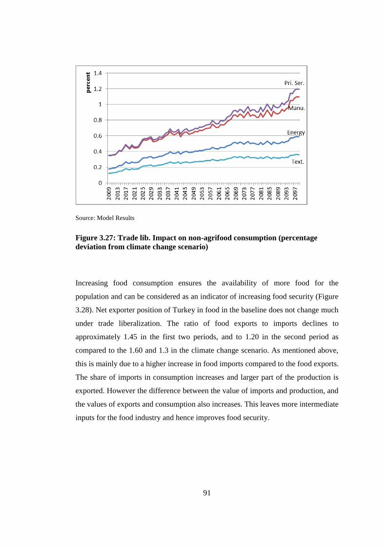
91

Source: Model Results

Figure 3.27: Trade lib. Impact on non-agrifood consumption (percentage

deviation from climate change scenario)

Increasing food consumption ensures the availability of more food for the

population and can be considered as an indicator of increasing food security (Figure

3.28). Net exporter position of Turkey in food in the baseline does not change much

under trade liberalization. The ratio of food exports to imports declines to

approximately 1.45 in the first two periods, and to 1.20 in the second period as

compared to the 1.60 and 1.3 in the climate change scenario. As mentioned above,

this is mainly due to a higher increase in food imports compared to the food exports.

The share of imports in consumption increases and larger part of the production is

exported. However the difference between the value of imports and production, and

the values of exports and consumption also increases. This leaves more intermediate

inputs for the food industry and hence improves food security.

92

Source: Model Results

Figure 3.28: Food security indicators (percentage deviation from climate

change scenario)

3.4 Conclusion

In this chapter we analyzed the effects of elimination of tariffs imposed on

agricultural imports from EU under a climate change. For this purpose we simulated

climate change and trade liberalization scenarios, by taking into account possible

effects of climate change on world prices. The results show that climate change can

cause a GDP loss as high as 3.5 percent. Main drivers of the loss in GDP due to

climate change are the significant decline in private consumption, and up to two

percent increase in imports.

Elimination of tariffs on imports from EU alleviates the negative effects of climate

change only marginally for Turkey as is the case for many other regions in the

world. The increase in welfare due to trade liberalization is very small compared to

the loss caused by climate change. However, benefits from trade liberalization

increases as the climate change effects worsen, especially after 2060. This is due to

93

the fact that under trade liberalization the economic agents have more substitution

possibility both in production and consumption.

Main adjustment mechanism of the economy under trade liberalization works

through the substitution intermediate goods with factors of production, as well as

substitution of domestic goods with imported goods. This causes significant

changes at the sectoral level. Wheat, rice and cereals are the most affected

commodities from trade liberalization, under climate change. They lose

competitiveness against alternative commodities both in domestic and international

markets, since the climate change reduces their yields substantially. Their

production, exports and prices decline simultaneously and substitution of domestic

production with imports is highest in these commodities.

Maize, oilseeds, fruits and processed food benefit from trade liberalization. Their

production and exports increase, domestic prices decline while imports remain

unchanged or increase slightly. Factors of production are directed towards the

production of these commodities as they become relatively more competitive after

the climate shocks.

Imports from the EU27 countries increase significantly and this causes domestic

prices to decline in the trade liberalization scenarios. Consequently, production of

agricultural commodities falls. Since the decline in domestic prices is lower than the

tariffs imposed to the other trading regions, prices of agricultural imports from the

other regions increases. This causes aggregate imports to decline. Hence, trade

liberalization with EU causes an “overcrowding” effect and decreases imports from

other trading regions. Food consumption increases under trade liberalization. As a

result, trade liberalization increases food security.

The findings from the simulation exercises suggest that although overall welfare

effect of trade liberalization is limited, it increases the economy’s ability to adapt by

fostering reallocation of scarce domestic resources to more efficient sectors. This

occurs as imports and domestic commodities become more substitutable.

94

The analysis in this chapter provides several paths for the improvement of the

model’s structure and scenario design. For instance, other countries will also be

affected by the climate change, and this is likely to be reflected in their demand for

Turkish commodities and their supply of commodities to Turkey. This can change

the implications of climate change and trade liberalization for Turkey. Secondly,

bilateral trade liberalization with the EU is not the only policy option for Turkish

policy makers. Trade liberalization with the other countries/regions can have

amplified effects. Lastly, analysis in this chapter uses the results of only one GCM

to calculate the economic shock parameters; however various estimates by different

GCMs are available. The results can be altered by different climate change

scenarios reported by different GCMs. In the next chapter, we will extend our

analysis to the global scale to compare various trade policy alternatives for Turkey

by taking into account the results of different GCMs.

95

CHAPTER 4

4. TRADE POLICY AS A GLOBAL ADAPTATION

MEASURE TO CLIMATE CHANGE

Simplicity is the ultimate sophistication.

Leonardo da Vinci

The physical effects of climate change in different parts of the world will depend on

various factors including geographic location, soil type, and land use pattern.

Nevertheless, the atmosphere is globally shared making climate change a global

issue. The outcome of the climate change include more frequent heat waves,

droughts, extreme precipitation, and related impacts (such as wild fires, heat stress,

vegetation changes, and rising sea level); all of which will be regionally dependent

(Karl et al., 2003). The impact on a country’s economy will differ according to the

country’s mitigation and adaptive capacity which is in turn determined by many

economic and social factors including its development status, income distribution,

structure of production, and integration to the international markets. Hence the final

impact of climate change will be determined by the interaction of various regional

effects throughout the world. One important link for this worldwide complex

interaction is international trade. The effects in a country can be spread to other

regions or can be accommodated for by the international markets. Thus, to

complement our analysis in the previous chapters, we extend our analysis to see

how the relationship between trade liberalization and climate change would change

when taking into account these global dynamics.

96

Economic effects of climate change at the global level have been the topic of a vast

literature. Various methods have been employed to translate the physical effects to

economic shocks. The most popular way has been through the introduction of

climate change shocks to the agricultural sector as changes in yields and/or

irrigation requirements. Although no consensus has been reached in these studies,

some general results can be derived. The results suggest an average negative

welfare effect between one percent to two percent of GDP at the global level

(Calzadilla et al., 2010; Tol, 2012). The effects are generally considered weak due

to the smoothing of economic adaptation (Arndt, Chinowsky, et al., 2012; Bosello

et al., 2010). They display some diversity depending on location, time, sectors and

social groups. Country level analyses suggest more significant effects, both positive

or negative, especially in the Middle East (Sowers et al., 2010; World Bank, 2010),

Africa (Arndt, Farmer, et al., 2012; Pauw et al., 2010; Thurlow, Dorosh, et al.,

2012; Thurlow, Zhu, et al., 2012) and South Asia (Thurlow, Dorosh, et al., 2012).

The impact of climate change depends highly on the adaptive capacity of the social

groups or countries considered. Crop pattern, long-run assets such as physical

infrastructure, investment capacity in adaptation measures are reported to be

important factors (Arndt, Chinowsky, et al., 2012). Poor people and small farmers,

as well as most developing countries are more vulnerable to adverse effects

(Bosello et al., 2005; Thurlow, Zhu, et al., 2012). Sectoral effects are also diverse.

Most studies report negative effects on agriculture (Bosello et al., 2005; Calzadilla

et al., 2010; Nelson et al., 2009; Rosegrant et al., 2008), while some (Tol, 2012)

present possible positive effects. The effect on agriculture is mostly felt through

water availability (Nelson et al., 2009). Hence drought resistance of major crops

grown in a region, cropping pattern and farm structure are important in determining

final effects on agriculture. The effects can vary, not only among different crops,

but also among different varieties of the same crop (Thurlow, Dorosh, et al., 2012).

Negative effects on agricultural production bring about food security concerns

(Arndt, Farmer, et al., 2012; Calzadilla et al., 2011; Dell et al., 2008; Nelson et al.,

2009; Rosegrant et al., 2008). Poorer households (Thurlow et al., 2009) and urban

97

population (Pauw et al., 2010) are hit the hardest by food shortages under climate

change. Child malnutrition is likely to increase with declining calorie intake

(Nelson et al., 2009; Rosegrant et al., 2008).

The link between trade liberalization and climate change has been the analyzed by a

few studies. The main argument in the literature is that trade liberalization can

alleviate the negative effects of climate change by boosting international trade.

Trade liberalization is reported to have welfare-improving effects (Calzadilla,

Rehdanz, & Tol, 2011; Chen, McCarl, & Chang, 2012; Laborde, 2011; Reilly &

Hohmann, 1993). However these effects are generally weak and are not sufficient to

compensate for adverse effects of climate change (Randhir & Hertel, 2000; Reilly

& Hohmann, 1993). Welfare gains from trade liberalization depend on the

elimination of production and export subsidies (Randhir & Hertel, 2000). The

effects are not uniform and depend on the geographic location (Calzadilla et al.,

2010; Reilly & Hohmann, 1993) and the vulnerability of the region to climate

change (Reilly & Hohmann, 1993). Changes are expected to affect more the poor

people (Laborde, 2011). The studies that consider the effects of trade liberalization

under climate change do not report any specific results or implications for Turkey.

In this chapter we will analyses the effects of climate change at the global level and

evaluate the effects of various trade policies as an adaptive measure by using the

GTAP model. GTAP is a detailed global CGE model that is used extensively in the

literature for trade policy analysis. Our version has 16 regions and 15 activities that

are aggregated from the GTAP 7 database. We follow the same approach adopted in

Chapter 3. We first introduce yield shocks based on 25 different climate projections

to obtain our baseline and then analyses the consequences of different trade

liberalization scenarios by benchmarking the simulation results to these baselines.

The rest of the chapter is organized as follows: Section 4.1 summarizes the

modelling approach and data. Then, a detailed description of scenarios follows. In

section 4.3 we present the simulation results. The final section is reserved for

concluding remarks.

98

4.1 Modelling framework: GTAP Model

GTAP is a multi-regional global static CGE model that represents the behavior of

households, producers and governments in each region following the standard

assumptions of the general equilibrium theory. Figure 4.1 shows the basic structure

of consumption and production in GTAP model. Households are utility maximizing

agents that receive all income generated in the economy. They spend it on private

consumption and save according to a Cobb-Douglas utility function. Income is

generated by skilled and unskilled labor, land, capital and natural resources that are

owned by households as endowments. Private consumption is distributed between

different commodities according to a non-homothetic Constant Difference of

Elasticity (CDE) implicit expenditure function, while government consumption is

distributed by a Cobb-Douglas function. Government consumption decision is done

by households’ utility maximization decision. Therefore tax revenues return back to

households as income. Households also consume imported commodities both for

private and government consumption. Imported commodities are bought directly

from the rest of the world. The consumption of imports is modeled with Armington

specification. Hence imports and domestic consumption are not perfect substitutes.

The saving decisions of household are made at the same time as their consumption

decisions. The sum of the savings accumulated by the households in all regions is

distributed among regions and sectors according to the price of capital. Hence,

savings drive investments and the model closure is essentially neo-classical in

nature. Investments change only the capital stock of the sectors and are not related

to technological change or productivity.

Producers are profit-maximizing agents that produce various commodities

according to a Constant Elasticity of Substitution (CES) production function by

using intermediate inputs and factors supplied by households. Firms use both

domestic and imported intermediate inputs and the substitution between these two

follows the Armington specification.

99

Source: GTAP (2011)

Figure 4.1: Structure of consumption and production in GTAP Model

A detailed documentation of the model can be found in (Hertel, 1997) and

(Brockmeier, 1996). A graphical representation of the GTAP model structure can be

found in the Appendix Figure D.1. We use GTAP database Version 7 that consists

of bilateral trade, protection and transport data as well as national accounts of 113

regions that spans the entire world for the year 2004. We also used the Land Use

Data Base9 of GTAP, which consists of a disaggregation of agricultural production

and a harvested area by agro-ecological zones (AEZ). It covers 57 sectors, four

types of factors and one type of household. Turkey is represented as a single region

in GTAP database. For this study, we aggregated the data of 16 regions and 15

sectors (see Table 4.1) to keep the analysis focused on Turkey.

9 Land use data is based on FAO’s 2004 data on production, harvested area and price. The AEZ

structure is based on the SAGE database which consists of 6 categories identified by the length of

growing period (LPG), and divides the world into three climatic zones, namely: tropical, temperate,

and boreal.

100

Table 4.1: Regional and sectoral aggregation in the GTAP model

Regions Sectors

Oceania Paddy, rice

East Asia Wheat

Southeast Asia Coarse grains

South Asia Vegetables, Fruits

Canada Oilseeds

United States Sugar crops

Rest of Latin America Other crops

Brazil Dairy, Livestock

OECD Europe Extract

Rest of the Middle-East Vegetable oil

Eastern Europe Other processed food

Former-USSR Textile, Apparel

Turkey Manufactures

Rest of North Africa Utilities, Construction

Morocco Services

Sub-Saharan Africa

4.2 Scenario Design

We simulate four scenarios to analyze the effects of trade liberalization under

climate change. We first simulate a set of baseline scenarios (BASE) for each

climate projection and introduce only the climate change shocks. Then we run three

trade liberalization scenarios for each one of these baselines: Bilateral trade

liberalization between EU and Turkey (EU); world-wide trade liberalization in

agriculture (AGRI); and world-wide trade liberalization in all commodities

(FULL)10

.

Quantification of the physical effects of the climate change is accomplished

generally by using General Circulation Models (GCMs) that incorporate various

10 We also simulated agricultural trade liberalization with EU scenario but we will not present the

results here, since they are not very different from the full trade liberalization with EU scenario.

Negligible difference between the two scenarios is due to already low protection on non-agricultural

products because of the Customs Union Decision. See Chapter 3 for details.

101

global climate scenarios. There are several GCMs that try to project the future state

of the climate at the global level (Randall et al., 2007). However, the results and

conclusions of different GCMs diverge substantially (Fischer et al., 2005;

Schönwiese et al., 1987; Stern, 2006). One can think of these different results as a

description of different probable futures. If we imagine the realized future as a draw

from a probability distribution, then the results of different GCMs can be

considered as a sampling from this probability distribution which is defined by the

mean and variation of the main climatic variables such as temperature and

precipitation. Since the yield estimates are functions of these climate variables, they

can also be considered as stochastic variables that also come from a probability

distribution. Consequently, using the results of as many GCMs as possible will

increase the accuracy of the estimates by making it possible to span a large number

of probable futures.

The set of scenarios that are used by GCMs creates another source of variability in

the state of future climate. These scenarios are generally composed of various

assumptions about the economy (GDP and population growth, consumption and

production patterns, energy use, GHG emissions etc.) and society (political systems,

international relations, culture, life style etc.). Assumptions are generally supported

by a storyline that is, in turn, backed up by expert opinion and/or results of various

qualitative or quantitative analyses. Hence, even if only one GCM is used, each

simulated scenario will provide results that would reflect one draw from the

probability distribution of future state of the global climate. The most popular set of

scenarios about the future state of the world are developed by IPCC emission

scenarios (Bates et al., 2008).

Following this line of reasoning, we collected estimates of future yield changes

caused by climate change from two different sources: IFPRI Food Security CASE

Maps database (IFPRI, 2012) and the Integrated Model to Assess the Global

Environment (IMAGE) Project’s database (IMAGE Team, 2009). Both sources use

an integrated approach to derive yield changes from the results of different GCMs

under different climate scenarios. The IFPRI database provides global projected

102

yield impacts for six crops (rice, wheat, maize, cassava, groundnut, and soybean)

with a wide range of scenario specifications for five year increments over a period

ending in 2050. The effects of climate change are translated to yield shocks by

using a biophysical model. The climate scenarios introduced to the crop model

follow from two different GCMs (namely CSIRO and MIROC) used to simulate

pessimistic, optimistic and normal versions of A1B and B1 SRES scenarios. The

database also supplies results of pessimistic, optimistic and normal versions of a

perfect mitigation scenario. Hence IFPRI database contains yield estimates for 15

different probable futures. A detailed description of the models and the database can

be found in Nelson et al. (2010).

The IMAGE database provides global yield impacts for 14 crop categories under

four SRES scenarios (A1B, B1, A2, and B2), and covers 17 regions/countries until

2100. The projected yield impacts are generated via terrestrial models in the

IMAGE framework which are coupled to the LEITAP model, by using input data

such as CO2 concentration, cloudiness, temperature and precipitation as projected

under each SRES climate scenario. IMAGE contains the impact of 10 different

climate change scenarios. Detailed description can be found in Hoogwijk et al.

(2005) and Bouwman et al. (2006).

The autonomous productivity growth, which exists in both models as an exogenous

TFP increase, is deducted from the yield change estimates. The regional and crop

dimensions of the yield shocks calculated from these databases are aggregated to

synchronize them with the dimensions of GTAP. We used average yield changes

weighted according to the production area of different crops in different regions.

We also treated the change in the yields of irrigated activities separately by giving a

relatively higher share to them in the weighting.

The distribution of yield changes for Turkey under all climate scenarios is given in

Figure 4.2. Average yields of oilseeds, wheat and other crops decline while the

average yields of rice, other grains and vegetables and fruits increase. The increase

in average value is quite susceptible due to high variability in the yield changes of

103

these crops in different climate scenarios. For grains, the minimum change is

around -35 percent, while it is lower than -20 percent for vegetables and fruits. The

variability in yield change is generally higher for Turkey compared to the EU and

the world averages, except for wheat. However the distribution is right skewed for

all crops except rice which means that the probability of optimistic scenarios is

higher.

Source: Authors’ Calculation from Hoogwijk et al., (2005) and Bouwman et al., (2006)

Figure 4.2: Distribution of yield changes for Turkey, EU and World

(percentage change)

Yield changes for the EU are generally negative but less volatile. Thus, Turkey is

likely to be affected more by climate change compared to the rest of the world. The

distributions of yield changes for the other regions are given in Figure D.2. The

estimates are in line with the expectations, in the sense that adverse effects on

Africa and Middle East are higher compared to the other regions while Oceania and

Canada turns out to be benefiting from climate change in terms of yield changes.

104

We introduce these yield changes as productivity shocks to the respective sectors

and regions. The results are then used to obtain 25 different baselines, which in turn

are used as the benchmark of the trade scenarios. Trade liberalization scenarios are

run on top of each baseline separately to obtain 25 different results for each trade

scenario. The first trade scenario is based on bilateral tariff elimination between

Turkey and European countries. Then we simulate global trade liberalization in

agricultural trade by eliminating tariffs imposed in all regions on agricultural

commodities. Lastly, we eliminate all tariffs imposed on all commodities by all

regions to analyze the effects of a full global trade liberalization scenario.

Table 4-2: Summary of scenarios

Trade scenario

Description

BASE Climate change only

EU Climate change + Tariff elimination on all tradable commodities between OECD Europe + Eastern Europe and Turkey

AGRI Climate change + Global tariff elimination on all agricultural tradable commodities

FULL Climate change + Global tariff elimination on all tradable commodities

4.3 Results and discussions

4.3.1 Effects of Climate Change

The distribution of the equivalent variation (EV) is given in Figure 4.3 as a box

plot11

for all regions. The global EV varies quite significantly for the different

11 The vertical line at the end of spikes shows the upper and lower adjacent values. The box covers

25th

and 75th

quintiles. The white line inside the boxes shows the value of median. The dots outside

the spikes show outliers.

105

climate change scenarios. The minimum is about a $20 billion loss, while the

maximum is as high as a $40 billion gain. The median of world EV is reduced to

about a $9 billion loss12

when the two extreme outcomes are considered as outliers.

The maximum welfare loss is around 0.1 percent of the global consumption, which

is also small. However, it is important to note that the world EV is sum of the EV

for different regions, and therefore a small impact at the global level does not

necessarily imply negligible effects at the regional/country level. For example, for

Turkey and the EU maximum welfare losses are around 0.3 percent of initial

consumption level, which is much higher than the global average. East Asia and

Europe are the most adversely affected regions. In all regions, the median EV is

generally negative except South Asia and South America. On the other hand, for

Sub-Saharan Africa13

, South Asia and Latin America almost the whole distribution

is above zero implying a high probability of welfare gains for these regions. These

regions are actually benefiting from climate change and the productivity shocks

implemented to the agricultural production of these regions is generally positive

(see appendix Figure D.2). For the rest of the regions the distribution of the EV

spans both negative and positive values, suggesting an uncertain outcome but the

distribution is not very dispersed and is centered around zero.

12 This corresponds to 0.04 percent of the initial world consumption.

13

The performance of GCMs is quite questionable for Sub-Saharan Africa. Precipitation projections

which are the main driver of the change in yields are particularly unreliable. Hence the positive

effects in Sub-Saharan Africa can be due to the bias in GCMs. A comparative analysis of

controversial results of different GCMs in Sub-Saharan Africa can be found in Müller (2009).

106

Source: Model Results

Figure 4.3: Distribution of EV for all regions in the model under baseline

scenarios (USD million)

Changes in regional GDPs are more significant and have more disperse

distributions (Figure 4.4). GDPs in South Asia and Sub-Saharan Africa increase

under all climate scenarios, while the impact is small for USA, Europe and the

Former USSR countries. The benefits from climate change are high for the former

group while agriculture constitutes a relatively smaller part of the economy in the

latter. However for Oceania, East and South East Asia the median value for the

GDP change is slightly negative although the absolute value of positive changes in

GDP are higher than the absolute value of negative changes. In Middle East and

North Africa (including Turkey), the change in the median value is slightly positive

but the negative changes are higher than the positive changes in absolute terms.

-40,0

00

-20,0

00

0

20,0

00

40,0

00

BA

SE

Oce EAs SEAs SAs Can USA XLA Bra EU XME EEur XRus Tur NAf SSAfr World

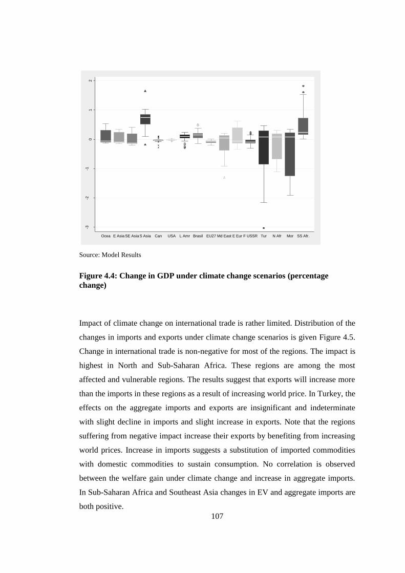
107

Source: Model Results

Figure 4.4: Change in GDP under climate change scenarios (percentage

change)

Impact of climate change on international trade is rather limited. Distribution of the

changes in imports and exports under climate change scenarios is given Figure 4.5.

Change in international trade is non-negative for most of the regions. The impact is

highest in North and Sub-Saharan Africa. These regions are among the most

affected and vulnerable regions. The results suggest that exports will increase more

than the imports in these regions as a result of increasing world price. In Turkey, the

effects on the aggregate imports and exports are insignificant and indeterminate

with slight decline in imports and slight increase in exports. Note that the regions

suffering from negative impact increase their exports by benefiting from increasing

world prices. Increase in imports suggests a substitution of imported commodities

with domestic commodities to sustain consumption. No correlation is observed

between the welfare gain under climate change and increase in aggregate imports.

In Sub-Saharan Africa and Southeast Asia changes in EV and aggregate imports are

both positive.

-3-2

-10

12

Ocea E Asia SE Asia S Asia Can USA L Amr Brasil EU27 Md East E Eur F USSR Tur N Afr Mor SS Afr.

108

Overall, the welfare impact of climate change is negative for most of the regions but

more pronounced in East Asia and Europe. The variation across the climate

scenarios is high implying a significant degree of uncertainty. In South Asia, Sub-

Saharan Africa, and Latin America welfare is improved mostly due to increasing

imports and exports. Global trade liberalization improves the welfare of all regions

and partially alleviates the negative effects for most of them.

Source: Model Results

Figure 4.5: Change in aggregate imports and exports under climate change

scenarios (percentage change)

-10

12

34

-10

12

34

Ocea E Asia S E Asia S Asia Can USA L Amer Bra EU27 Md East E Eur F USSR Tur N Africa Mor SS Afr.

Ocea E Asia S E Asia S Asia Can USA L Amer Bra EU27 Md East E Eur F USSR Tur N Africa Mor SS Afr.

Exports

Imports

Graphs by type

109

4.3.2 Effects of Trade Liberalization

The distribution of welfare effects under trade liberalization and the baseline

scenarios for Turkey is given in Figure 4.6. Firstly, note that the variation in EV is

very small across the different baselines. Hence, the effect of trade liberalization on

welfare is independent of the selected climate scenario. The effects of trade

liberalization scenarios are magnified with the extent of liberalization. The welfare

gain under the FULL scenario is higher than the negative effects of climate change

for almost 75 percent of the climate change scenarios. However, gains from AGRI

or EU scenarios are weak and hardly compensate for the losses observed under

most of the climate change scenarios. The variation in the EV is very small across

different climate change scenarios. Hence, welfare effect of trade liberalization is

independent of the selected climate scenario. The effects of climate change on

agricultural productivity do not change the structure of the global economy.

Source: Model Results

Figure 4.6: Distribution of EV for Turkey under all scenarios (million USD)

-8,0

00

-6,0

00

-4,0

00

-2,0

00

0

2,0

00

Turkey

EU AGRI FULL BASE

110

The EVs of Turkey’s major trading partners under trade liberalization are displayed

in Figure 4.7. The EV is generally positive under all trade liberalization scenarios

for Turkey. However, as expected this is not true for all countries and regions. For

example, gains for the USA from agricultural trade liberalization are close to zero

while they are negative under full trade liberalization. Gains in the EV for the EU,

East Asia and Middle East due to full trade liberalization are positive, and they are

likely to recover the losses caused by climate change at least for the 75 percent of

the climate scenarios.

Agricultural trade liberalization alleviates the welfare loss in East Asia. The effects

are limited for other regions. The effect of trade liberalization between the EU and

Turkey is also limited and hardly alleviates the negative impacts of climate change.

Source: Model Results

Figure 4.7: Distribution of EV for main trading partners of Turkey under

trade liberalization scenarios (million USD)

-26

,98

71

0,2

03

EU AGRI FULL BASE

EU27

-12

,33

85

8,8

36

EU AGRI FULL BASE

East Asia

-2,6

23

.94

,77

9.1

EU AGRI FULL BASE

East Europe

-2,3

43

.83

,45

5.8

EU AGRI FULL BASE

Former USSR

-11

,70

66

,16

1.8

EU AGRI FULL BASE

Middle East

-12

,24

23

,09

4.3

EU AGRI FULL BASE

USA

Graphs by reglng

111

The decomposition of the change in EV for Turkey according to the main drivers,

namely allocative efficiency, technological efficiency and terms of trade, is

presented in Figure 4.8. Contribution of changes in investment and saving to the

total EV is generally small. Under climate change, technological change is the

major contributor to the change in EV. This contribution is generally negative,

although the median value is slightly above zero. This is expected since climate

change scenarios are introduced as negative productivity shocks in the agricultural

sector. Terms of trade effect is generally driven by the changes in export prices for

Turkey (see appendix Figure D.10 for the decomposition of the terms of trade

effects). Under the AGRI scenario, the terms of the trade effect is negative. Since

Turkey is a net exporter of the agricultural products, declining world prices has a

negative terms of trade effect on the Turkish EV. However, the sign of terms of

trade effect is reversed under the FULL scenario as the positive effect of declining

world prices of the manufacturing and services trade dominates the negative impact

due to agricultural trade. Under the EU scenario, the effect of terms of trade effect

becomes positive and constitutes the largest part of the EV change. The effect is

again driven by the change in export prices. The allocative efficiency contributes

positively to the EV under the global trade liberalization scenarios since the

removal of tariffs eliminates a significant distortion. Under the AGRI scenario the

positive effect of allocative efficiency is higher than the negative effect of the terms

of trade effect. The contribution of allocative efficiency does not change much

under the FULL scenario. More than 80 percent of the contribution of allocative

efficiency is comes from other crops sector under both AGRI and FULL scenarios.

Other crops sector is heavily protected and has a significant share in the agricultural

trade. The most important difference between the two scenarios is observed in the

livestock and processed food sectors which form more than 25 percent of the

allocative efficiency contribution under the FULL scenario. However, allocative

efficiency declines due to the declining use of production factors under the FULL

scenario, while it increases under the AGRI scenario. These two opposing effects

cancel each other out and the contribution of allocative efficiency ends up being

close to zero. Under the EU scenario, the contribution of allocative efficiency to the

112

EV is insignificant, although it is slightly negative. The decline is mostly due to the

negative effects in the manufacturing and textile sectors. The highest positive

contribution comes from the processed food, vegetable oils and fruits & vegetables

sectors (see Appendix Figure D.9).

Source: Model Results

Note: Tech./Sav. Inv. shows effect of technological change for BASE and effect of investment

change for the other scenarios. Alloc. shows allocative efficiency effect and ToT shows terms of

trade effect.

Figure 4.8: Decomposition of EV for Turkey (million USD)

The change in Turkey’s GDP and those of her trading partners is given in Figure

4.9. Turkish GDP increases under the EU and the FULL scenarios while it declines

under the AGRI scenario. The change in GDP for third countries is negative under

the EU scenario as expected. For Turkey’s main trading partners, the changes in the

GDP are also insignificant under the AGRI scenario; only East Asia and the Former

USSR countries see a slight increase in their GDP. East Asia is the only region that

benefits from the FULL scenario together with Turkey. The increase in the East

-9,1

65.7

1,42

6.9

Alloc. Tech./Sav. Inv. ToT

BASE

-322

.86

1,12

2.2

Alloc. Tech./Sav. Inv. ToT

AGRI

-51.

9348

7.07

Alloc. Tech./Sav. Inv. ToT

EU

8.7

1,35

6.6

Alloc. Tech./Sav. Inv. ToT

FULL

Graphs by Scenarios

113

Asian GDP is greater than 1.5 percent. The rest of the regions see significant GDP

losses. The highest decline is noted for the former USSR countries with more than a

two percent decline.

Private consumption and trade are the main drivers of the change in GDP for

Turkey (Figure 4.10). The contribution of exports is positive while contribution of

imports is negative on the GDP implying a simultaneous increase in exports and

imports. Private consumption increases under the EU and FULL scenarios, while it

declines under the AGRI scenario. Under the EU scenario, although the effects are

small, the positive contributions of exports and consumption dominate over the

negative effect of imports and private consumption on the GDP. Furthermore, the

contribution of investments is positive and relatively high under the EU scenario.

This implies an increasing return of capital in Turkey after trade liberalization with

EU.

Source: Model Results

Figure 4.9: Average change in GDP for Turkey and her trading partners

(percentage change)

114

The decreasing contribution of private consumption to the change in the GDP under

the FULL scenario is the main reason for the smaller change in the GDP compared

to the one observed for the EU scenario. Under the AGRI scenario, private

consumption declines and together with the increasing imports, dominates the

positive effects of the increase in exports.

The immediate effect of tariff elimination for Turkey is the decline in world prices, which in turn

affects the import and export prices. Under the EU scenario, the decline in import prices is

negligible, while export prices increase, but the change is still under one percent. The increase in the

export prices of non-agri-food sectors is even smaller. The variation in the changes of export prices

over climate scenarios is given in Appendix Source: Model Results

Figure D.12. The variation is quite low for all products except rice, which is traded

thinly in the world, and also between the EU and Turkey.

Source: Model Results

Figure 4.10: Decomposition of GDP change for Turkey (difference from

baseline average, million USD)

115

Changes in the export and import prices are relatively higher under both the AGRI

and FULL scenarios. The changes are mainly driven by the change in the world

prices after the trade liberalization. Import prices increase for all sectors, except

vegetables & fruits, under both scenarios (Figure 4.11). Global scale trade

liberalization increases the world price for agricultural commodities. This is mainly

due to the increasing demand for agricultural products as intermediate inputs.

Increasing production (see Appendix Figure D.21) by the food, manufacturing and

services sectors shifts up the global demand for the agricultural commodities. Since

a significant part of agricultural imports is used as intermediate inputs (60 percent

to 95 percent), the demand for these commodities increases causing import prices to

increase. Domestically produced commodities substitute for the imports. This in

turn causes consumption to increase as the production in the other sectors that use

agricultural commodities as intermediate input increases, accompanied by a

decrease in the domestic prices. As a result the price of agricultural imports

increases. Note that for fruits and vegetables, a relatively smaller share of imports is

used as intermediate inputs with 35 percent, and hence the effect of tariff

elimination remains dominant for these products.

Source: Model Results

Figure 4.11: Average Change in Turkish import price index under trade

liberalization scenarios (percentage change)

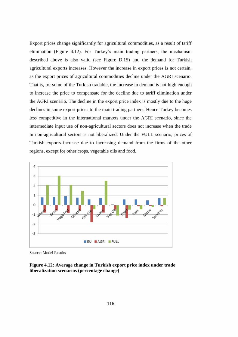
116

Export prices change significantly for agricultural commodities, as a result of tariff

elimination (Figure 4.12). For Turkey’s main trading partners, the mechanism

described above is also valid (see Figure D.15) and the demand for Turkish

agricultural exports increases. However the increase in export prices is not certain,

as the export prices of agricultural commodities decline under the AGRI scenario.

That is, for some of the Turkish tradable, the increase in demand is not high enough

to increase the price to compensate for the decline due to tariff elimination under

the AGRI scenario. The decline in the export price index is mostly due to the huge

declines in some export prices to the main trading partners. Hence Turkey becomes

less competitive in the international markets under the AGRI scenario, since the

intermediate input use of non-agricultural sectors does not increase when the trade

in non-agricultural sectors is not liberalized. Under the FULL scenario, prices of

Turkish exports increase due to increasing demand from the firms of the other

regions, except for other crops, vegetable oils and food.

Source: Model Results

Figure 4.12: Average change in Turkish export price index under trade

liberalization scenarios (percentage change)

117

The volume of trade of agricultural commodities changes significantly under all

scenarios. Exports in agricultural commodities increase in line with the change in

export prices under the EU scenario (Figure 4.13). The most important increase in

exports is observed in wheat, grains and vegetable oils. Exports of vegetable oil

triple under the EU scenario and the increase for wheat and grains is also quite

significant with increases reaching 105 percent and 68 percent respectively. The

increase is mostly due to increasing trade with the EU. Vegetable oil exports from

Turkey to the EU27 countries are heavily protected. Food exports also increases

around 20 percent. On the other hand, exports in non-agrifood sectors decline by

around two percent. The most important increase is observed for vegetables &

fruits, wheat, vegetable oils and processed food with increases ranging from 20

percent to 30 percent.

Agricultural imports are mostly used as intermediate inputs. Hence, the change in

agricultural imports is mainly driven by the increasing intermediate input demand.

However it is important to note that the increase in imports under the EU scenarios

is significant only for the commodities that become cheaper than their domestic

counterparts. Wheat, vegetable & fruits, vegetable oils and food are the most

important among these commodities. The increase in these commodities is mainly

driven by the boosting of production of grains, livestock products and vegetable

oils.

118

Source: Model Results

Figure 4.13: Change in Turkish imports and exports under the EU scenario

Exports of wheat, grains, oilseeds and other crops increase significantly under the

AGRI scenario (Figure 4.14). However, this increase is accompanied by a decline in

export prices, implying that Turkey is non-competitive in these commodities on the

global scale. Declining domestic prices in most regions (see Appendix Figure D.20)

forces Turkey to export at lower prices. Turkey is able to increase exports even with

decreasing prices. Note that exports of vegetables and fruits decline due to small

changes in domestic prices. Trade in livestock, vegetable oil and food sectors do not

change significantly as domestic and imported commodities are not substitutable

due to the low trade levels reflected in the baseline. Imports of agricultural

commodities also increase significantly, this time as substitutes for domestic

production. This is caused by declining domestic prices, which inevitably cause

production to decline.

119

Source: Model Results

Figure 4.14: Change in Turkish imports and exports under AGRI scenario

The effects of full global trade liberalization are quite significant (Figure 4.15).

Under the FULL scenario, exports of livestock, vegetable oil and food increase by

almost 200 percent. This causes a significant increase in the domestic production of

these commodities, which in turn causes an increase in imports needed as

intermediate inputs. The increase in imports is higher in vegetable & fruits than the

rest, mostly due to the increase in intermediate input use from the food sector.

Wheat, sugar and other crop imports also increase since the livestock and food

processing sectors use them extensively. The ‘Trade opening’ effect is also

observed under the FULL scenario in the sense that, declining domestic prices and

increasing export prices makes exporting more appealing for the producers.

120

Source: Model Results

Figure 4.15: Change in Turkish imports and exports under FULL scenario

The change in consumption is relatively modest compared to the change in trade

(Figure 4.16). This is not surprising considering the fact that trade is mostly driven

by intermediate input use. Change in consumption of agricultural commodities is

insignificant under the EU scenario. The consumption of agricultural commodities

increases significantly under the AGRI and the FULL scenarios. The increase in the

consumption of food, livestock commodities and vegetable oils as well as non-

agrifood commodities are very high under the FULL scenario compared to the

changes in consumption of these commodities under AGRI scenario. This is mainly

due to the increase in imports of these commodities and underlies higher welfare

gains. Note that without the trade liberalization in the textiles and manufacturing

sectors, the consumption of these commodities does not increase at all. This

suggests that cheaper intermediate inputs are not enough to make these sectors

competitive in the international markets, but the elimination of tariffs has an

important role in sustaining the competitiveness of these sectors.

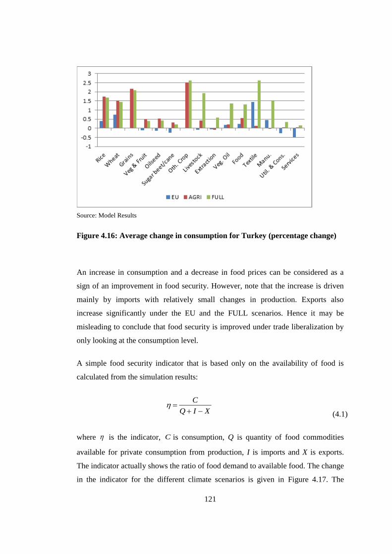
121

Source: Model Results

Figure 4.16: Average change in consumption for Turkey (percentage change)

An increase in consumption and a decrease in food prices can be considered as a

sign of an improvement in food security. However, note that the increase is driven

mainly by imports with relatively small changes in production. Exports also

increase significantly under the EU and the FULL scenarios. Hence it may be

misleading to conclude that food security is improved under trade liberalization by

only looking at the consumption level.

A simple food security indicator that is based only on the availability of food is

calculated from the simulation results:

(4.1)

where is the indicator, is consumption, Q is quantity of food commodities

available for private consumption from production, I is imports and X is exports.

The indicator actually shows the ratio of food demand to available food. The change

in the indicator for the different climate scenarios is given in Figure 4.17. The

C

Q I X

C

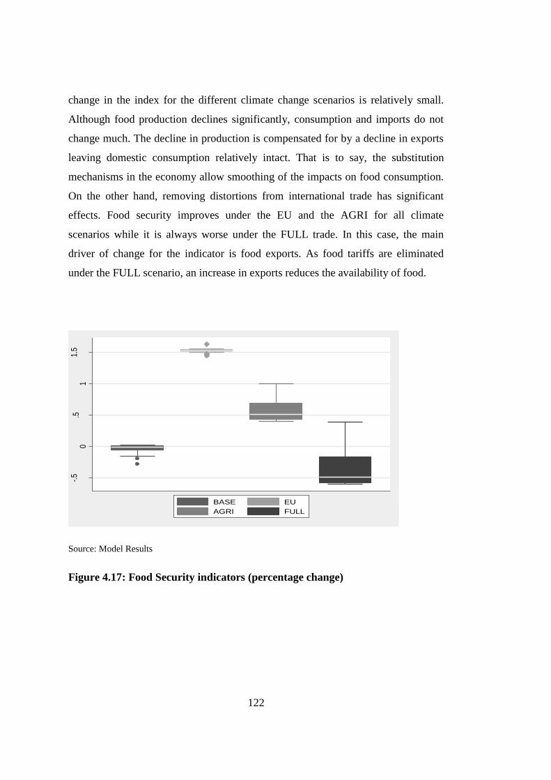
122

change in the index for the different climate change scenarios is relatively small.

Although food production declines significantly, consumption and imports do not

change much. The decline in production is compensated for by a decline in exports

leaving domestic consumption relatively intact. That is to say, the substitution

mechanisms in the economy allow smoothing of the impacts on food consumption.

On the other hand, removing distortions from international trade has significant

effects. Food security improves under the EU and the AGRI for all climate

scenarios while it is always worse under the FULL trade. In this case, the main

driver of change for the indicator is food exports. As food tariffs are eliminated

under the FULL scenario, an increase in exports reduces the availability of food.

Source: Model Results

Figure 4.17: Food Security indicators (percentage change)

-.5

0.5

11.

5

BASE EU

AGRI FULL

123

4.4 Conclusion

The results suggest that the impact of climate change on the global economy spans a

wide range of probabilities. Effects can be either positive or negative depending on

the size and characteristics of the physical effects, although the probability of

observing negative effects is higher. The final effect is determined by a complex set

of interactions among different regions of the world and sectors within these

regions. This increases the level of uncertainty making the climate risk vital when

evaluating possible impacts of different adaptation measures.

Economic impacts of climate change differ significantly among regions. Sub-

Saharan Africa and South Asia are the only benefiting regions in terms of economic

welfare while Europe, Middle East and North Africa are affected adversely. On the

other hand for East Asia and Europe, the variation in the results for the different

climate scenarios is very high. Hence for Europe, the effects of climate change are

likely to hamper the welfare significantly.

The variation in the effects of climate change over different climate scenarios is not

fully reflected in the macroeconomic variables. For most regions the changes in

GDP are scattered around zero. The disperse distribution of GDP shows the

contribution of economic interactions to the climate risk. The most affected regions

are small economies that are in the vulnerable regions such as Turkey, Morocco,

Middle East, and North African countries.

The most important conclusion of the simulation results is that the negative welfare

effects of climate change can be alleviated by trade liberalization for most parts of

the world. The increase in welfare under a full trade liberalization scenario is higher

than the loss under the climate change scenarios. However, regional trade

liberalization such as tariff elimination between Turkey and EU does not alleviate

the effects of climate change.

Turkey can alleviate the negative welfare effects of climate change through the

implementation of global trade liberalization policies. Furthermore, the Turkish

124

GDP increases after trade liberalization implying a relatively higher increase in

exports compared to imports. Actually, the change in the GDP under trade

liberalization is driven mainly by imports and exports. The effects of trade

liberalization on Turkey are mainly through the imported intermediate input use.

Although effects on sectors may differ, Turkish imports generally increase to

accommodate the increased demand of intermediate inputs by exporting sectors,

thus in turn resulting in an increase in exports. Imports of agricultural commodities

increase to supply the intermediate input demand by food, manufacturing, livestock

and vegetable oil sectors thus boosting production and in turn exports.

The effect of trade liberalization on food security is sensitive to the climatic

conditions, although the variation in sectoral results across climate scenarios is

generally low. The worse the effect of climate change is, the more the food security

is improved by trade liberalization. This is mainly due to the increase in imports and

decline in exports under severe climate conditions since domestic production

declines significantly under more pessimistic climate scenarios.

The availability of food is generally determined by the export demand for Turkish

food commodities. As domestic prices decline due to tariff elimination, Turkish

exports increase putting pressure on the availability of food supply for domestic

consumption. On the other hand, increasing food imports decreases this pressure by

increasing the amount of available food. Food security improves the most after the

liberalization of trade between Turkey and the EU as export pressure on domestic

food availability is decreased. Under full global trade liberalization the increase in

production and imports is not sufficient to compensate for the effect of increasing

food exports.

125

CHAPTER 5

5. CONCLUDING REMARKS

Climate change is likely to be one of the most vital issues in the following decades.

The urge for adaptation is obvious. However, it is not costless and involves various

trade-offs between generations, regions, countries and social groups. This thesis is

an attempt to shed some light on the potential costs and trade-offs. In addition, an

overall picture of the interaction of the economy with climate change through the

agricultural sector is presented. The study considered the interactions among

economic agents at the regional and national level for Turkey as well as the global

dynamics that Turkey can face through-out the next century. An integrated

approach that uses a crop-water requirement model together with three CGE models

at regional, national and global levels was adopted to achieve this purpose.

The findings suggest that the effect of climate change on agricultural production is

likely to increase over time. The results show that the effects of the climate change

are likely to vary depending on the period. The first period lasts until 2030s, and

Turkish agriculture is likely to benefit from the climate change with increasing

average yields and declining irrigation requirements in this period. The second

period starts after the first period and extends until 2060s. The frequency of

negative climatic extremes increases significantly, although the average yield and

irrigation requirements deteriorate only slightly over this period. The last period

starts in 2060s and lasts until the end of the time-scope for the analysis, 2099. The

frequency of extreme negative climatic events continues to increase and the average

conditions deteriorate significantly. Consequently, last period witness a drastic fall

in agricultural yields and increase in irrigation requirements.

Effects on Turkish regions are quite diverse. Eastern parts of the country are

affected less while the western and southern coastal regions are hit the most.

126

Western parts of the country are relatively better off in the first period, and

relatively worse of in the following periods. This is mostly due to the relatively

higher importance of irrigation in these regions. In the absence of the adequate

water supply, the increasing price of irrigation water causes production to decline

drastically in these regions. On the other hand, eastern and southern regions are

affected less from the increasing irrigation water prices since the share of irrigated

activities is relatively lower.

Similar trends are observed at the national level. In the first period change in GDP

is between -0.1 and 0.7 with mostly positive GDP growth. GDP change remains

between -0.5 and 0.5 with more frequent negative changes in the second period. In

the last period, GDP growth is always negative between -0.5 and -3.5 percent.

Changes in EV vary between -3.3 percent and +1.3 percent of the household

consumption under climate change. Imports are reduced substantially while there is

a boost in exports, mainly due to manufacturing sector. Liberalization of

agricultural trade with EU is likely to have a limited overall effect to alleviate the

adverse effects of climate change. Welfare gains are positive but not significant

enough to change the sign of the overall effects. On the production side, the total

value added does not change much from the climate change scenario implying a

limited feedback effect. The main drivers of change on the GDP are imports and

consumption. The positive effect of declining imports on the GDP is reduced by the

declining domestic demand under trade liberalization.

Introducing the global dynamics does not change the effects of trade liberalization

policies for Turkey. Effects of EU trade liberalization are still weak and far from

alleviating climate change effect. However, global trade liberalization can alleviate

the adverse effects for Turkey. The effects of global trade liberalization on Turkey

are mainly through the imported intermediate input use. Although effects on sectors

may differ, Turkish imports generally increase to accommodate the increased

demand for intermediate inputs by exporting sectors, thus resulting in an increase in

exports. Imports of agricultural commodities increase to supply the intermediate

127

input demand by food, manufacturing, livestock and vegetable oil sectors thus

boosting production and in turn exports.

The effect of trade liberalization on food security is sensitive to the climatic

conditions, although the variation in sectoral results across climate scenarios is

generally low. The worse the effect of climate change is, the more the food security

is improved by trade liberalization. This is mainly due to the increase in imports and

decline in exports under severe climate conditions since domestic production

declines significantly under more pessimistic climate scenarios.

Turkey still has time to take necessary adaptation measures. Prioritizing the

irrigation projects by taking into account the extent of regional impact of climate

change, investing in R&D activities to develop drought resistant crops, rationalizing

the irrigation water use by farmers, improving the integration of farmers to the

markets, enhancing the linkages between food and agricultural sectors, enriching

the links between agricultural markets in different regions can be considered as

policies to increase the resilience of the economy to the effects of climate change.

However, our analysis shows that any policy should be elaborated carefully for

costs and benefits. For example, trade liberalization can alleviate the negative

effects of the climate change only if implemented at the global scale. However,

regional trade liberalization can still contribute to adaptation efforts by relaxing the

constraints on consumption and on the supply of intermediate inputs.

The tools presented in this thesis can also be used to analyze many other adaptation

policy options by introducing relevant data into the model. For example, irrigation

policies can be introduced to the model in more detail to simulate the effects of

different water management strategies as an adaptation measure. Likewise, different

subsidy schemes can be simulated to see their effectiveness in climate change

adaptation and mitigation. Similarly, R&D investments can also be included in the

model to test if the technological development can create opportunities for

adaptation.

128

The analysis presented in the chapters of this thesis also paves the way for further

methodological improvements. For example, the modeling approach in second and

third chapters can be combined to analyze the effects of climate change at regional

level in a dynamic setting. Another possible improvement can be including more

household types in the model to extend the analysis to cover the distributional

effects of the climate change. Further, the model used in the last chapter can be

improved by including GHG emissions to see how adaptation through the trade

liberalization can affect the mitigation efforts to decreases GHG emission.

129

REFERENCES

Acar, M., Afyonoğlu, B., Kuş, S., & Vural, B. (2007). Turkey’s agricultural

integration with the EU: Quantifying the implications. 10th Annual Conference on

Global Economic Analysis, Purdue University, USA, June 7-9, 2007.

Adam, A., & Moutos, T. (2008). The trade effects of the EU–Turkey customs

union. The World Economy, 31(5), 685–700. doi:10.1111/j.1467-

9701.2008.01099.x

Agrawala, S., & Fankhauser, S. (Eds.). (2008). Economic aspects of adaptation to

climate change: costs, benefits and policy instruments. OECD Publishing. 1: 98–99

doi:10.3763/cdev.2009.0011

Alessandri, P. (2000). European and Euro-Mediterranean agreements: Some

simulation analysis on the effects of the EU trade policy. Centro Studi sui Processi

di Internazionalizzazione, Working Paper No: 110

Allen, R.G., Pereira, L.S., Raes, D., Smith, M., 1998. Crop evapotranspiration:

Guidelines for computing crop water requirements. Irr. Drain. Paper 56. UN-FAO,

Rome

Arndt, C. (1996). An introduction to systematic sensitivity analysis via Gaussian

quadrature, GTAP Technical Paper No. 2, Center for Global Trade Analysis,

Purdue University

Arndt, C., Chinowsky, P., Strzepek, K., & Thurlow, J. (2012). Climate change,

growth and infrastructure investment: The case of Mozambique. Rev. Devel. Econ.,

16(3), 463–475. doi:10.1111/j.1467-9361.2012.00674.x

Arndt, C., Farmer, W., Strzepek, K., & Thurlow, J. (2012). Climate change,

agriculture and food security in Tanzania. Rev. Devel. Econ., 16(3), 378–393.

doi:10.1111/j.1467-9361.2012.00669.x

Arslan-Alaton, I., Türkman, A., & Orhon, D. (2011). Climate change and its effects

on water resources. In A. Baba, G. Tayfur, O. Gündüz, K. W. F. Howard, et al.

(Eds.), Climate change and its effects on water resources issues of national and

global security (Vol. 3, pp. 285–292). Dordrecht: Springer Netherlands.

doi:10.1007/978-94-007-1143-3

130

Augier, P., & Gasiorek, M. (2003). The welfare implications of trade liberalization

between the Southern Mediterranean and the EU. Appl. Econ., 35(10), 1171–1190.

doi:10.1080/0003684032000081311

Aydınalp, C., & Cresser, M. S. (2008). The effects of global climate change on

agriculture. Am Eurasian J Agric Environ Sci, 3(5), 672–676.

Bates, B. C., Kundzewicz, Z. W.., Wu, S., & Palutikof, J. P. (2008). Climate change

and water. IPCC Technical Paper IV (pp. 1–220). Geneva: IPCC Secretariat.

Bayar, A., Diao, X., & Yeldan, E. (2000). Intertemporal, multi-region general

equilibrium model of agricultural trade liberalization in the South Mediterranean

NIC’s, Turkey, and the European Union. International Food Policy Research

Institute TMD Discussion Paper, (56).

Bekmez, S. (2002). Sectoral impacts of Turkish Accession to the European Union.

Eastern Europ. Econ., 40(2), 57–84.

Bosello, F., Eboli, F., & Parrado, R. (2010). Climate change impacts in the

Mediterranean: a CGE analysis. GTAP Working Paper, 5385.

Bosello, F., & Zhang, J. (2005). Assessing climate change impacts: Agriculture.

Fondazione Eni Enrico Mattei Nota di lavoro, 94.2005.

Bouwman, A. F., Kram, T., & Goldewijk, K. K. (2006). Integrated modeling of

global environmental change: An overview of IMAGE 2.4. Bilthoven: Netherlands

Environmental Assessment Agency (MNP).

Brockmeier, M. (1996). A graphical exposition of the GTAP model. GTAP

technical paper No. 8, Center for Global Trade Analysis, Purdue University, West

Lafayette, USA.

Bruinsma, J. (2003). World agriculture: Towards 2015/2030: an FAO perspective.

London: Earthscan.

Çağatay, S., Saunders, C., & Amor, R. (2001). The impact on the Turkish

agricultural sector of the potential extension of the CU agreement to cover

agricultural commodities. European Trade Study Group Third Annual Conference,

September 14-16, Brussels, Belgium,, 1–22.

131

Çakmak, E. H. (2007). Trade liberalization and turkish agriculture: Threat or

opportunity. Cal-Med Workshop IIII (Mediterranean Products in a …, 1–16.

Çakmak, E. H., & Kasnakoglu, H. (2003). The impact of EU membership on

agriculture in Turkey. Paper presented in Conference Femise, 4-6 December,

Marsilya France.

Calzadilla, A., Rehdanz, K., Betts, R., Falloon, P., et al. (2010). Climate change

impacts on global agriculture. Kiel Institute for the World Economy Working

Papers 1617, (1617).

Calzadilla, A., Rehdanz, K., & Tol, R. S. J. (2011). Trade liberalization and climate

change: A computable general equilibrium analysis of the impacts on global

agriculture. Water, 3(2), 526–550. doi:10.3390/w3020526

Calzadilla, A., Rehndaz, K., Betts, R., et al. (2013). Climate change impacts on

global agriculture. Climatic Change, 120:357-374. doi: 10.1007/s10584-013-0822-4

Chen, C.-C., McCarl, B., & Chang, C.-C. (2012). Climate change, sea level rise and

rice: global market implications. Climatic Change, 110(3-4), 543–560.

doi:10.1007/s10584-011-0074-0

Ciscar, J. C. (ed), Soria, A., Iglesias, A., Garrote, L., et al. (2009). Climate change

impacts in Europe: Final report of the PESETA research project. JRC Scientific and

Technical Reports, EUR 24093. doi:10.2791/32500

Cline, W. (2007). Global warming and agriculture: Impact estimates by country.

Peterson Institute for International Economics: Washington D.C.

Cretegny, L. (2009). The Economics of adaptation to climate change: An integrated

assessment framework. 12th Annual Conference on Global Economic Analysis,

Santiago, Chile, June 10-12.

Dalfes, H. N., Karaca, M., Sen, Ö. L., Kindap, T., et al. (2011). Türkiye için İklim

değişikliği senaryoları. Online Database. Retrieved May 18, 2011, from

gaia.itu.edu.tr

132

De Santis, R. (2000). The impact of a customs union with the EU on Turkey’s

welfare, employment and income distribution: an AGE model with alternative

labour market structures. Journal of Economic Integration, 15(2):195-238

Dell, M., Jones, B., & Olken, B. (2008). Climate change and economic growth:

Evidence from the last half century. NBER Working Paper No. 14132, NBER

Working Paper Series.

Dellal, İ., & Mccarl, B. (2009). The Economic Assessment of Climate Change on

Agriculture: US and Turkish Case. 1st International Congress on Global Climate

Change and Agriculture, 27-29 May, Tekirdag.

DeVuyst, E.A., Preckel, P.V., (1997). Sensitivity analysis revisited: A quadrature-

based approach, Journal of Policy Modeling, 19(2), 175–185

Diffenbaugh, N.S., Hertel T.W., Scherer, M. & Verma, M. (2012). Response of

corn markets to climate volatility under alternative energy futures, Nature Climate

Change, 2(7):514-517, doi: 10.1038/nclimate1491

Dudu, H., Çakmak, E. H., & Saraçoğlu, Ş. D. (2010). Climate change and irrigation

in Turkey: A CGE approach. İktisat İşletme ve Finans, 25(286), 9–33.

doi:10.3848/iif.2010.286.2577

Durdu, Ö. F. (2010). Effects of climate change on water resources of the Büyük

Menderes river basin, western Turkey. Turk J Agric For, 34, 319–332.

doi:10.3906/tar-0909-402

Eruygur, H. (2006). Impacts of policy changes on Turkish agriculture: an

optimization model with maximum entropy. Unpublished Ph.D thesis, Middle East

Technical University Department of Economics. Retrieved from

http://goo.gl/KOVIfI

Evans, J. P. (2005). Impact of global warming on the Euphrates-Tigris watershed.

Prooceedings of American Geophysical Union Fall Meeting, December (pp. 209–

218).

FAOSTAT. (2013) FAO statistics portal, trade database. Retrieved May 22, 2013,

from http://goo.gl/eIjY6S

133

Fankhauser, S. (2005). Valuing climate change: the economics of the greenhouse.

Earthscan: London.

Fellmann, T., Leeuwen, M. van, & Salamon, P. (2011). EU enlargement to Turkey:

Potential impacts on agricultural markets and how they are shaped by changes in

macroeconomic conditions. 51st Annual Conference of GEWISOLA, Halle 28-30

September 2011: Germany, 1–11.

Fernandes, E. C.M.; Soliman, A.; Confalonieri, R.; Donatelli, M. & Tubiello, F.

(2012). Climate change and agriculture in Latin America, 2020-2050 : Projected

impacts and response to adaptation strategies. World Bank, Washington, DC.

https://23.21.67.251/handle/10986/12582

Fischer, G., Shah, M., Tubiello, F. N., & Van Velhuizen, H. (2005). Socio-

economic and climate change impacts on agriculture: an integrated assessment,

1990-2080. Philosophical transactions of the Royal Society of London. Series B,

Biological sciences, 360(1463), 2067–83. doi:10.1098/rstb.2005.1744

Flegg, A., & Webber, C. (2000). Regional size, regional specialization and the FLQ

formula. Reg. Stud. 34(6): 563-569

Food and Agriculture Organization. (2011). CLIMWAT 2.0 for CROPWAT.

Online database. Retrieved from http://goo.gl/ghdeT

Francois, J. F., McQueen, M., & Wignaraja, G. (2005). European Union–

developing country FTAs: Overview and analysis. World Devel., 33(10), 1545–

1565. doi:10.1016/j.worlddev.2005.05.006

Fujihara, Y., Simonovic, S. P., Topaloğlu, F., Tanaka, K., et al. (2008). An inverse-

modelling approach to assess the impacts of climate change in the Seyhan River

basin, Turkey. Hydrological Sciences Journal, 53(6), 1121–1136.

doi:10.1623/hysj.53.6.1121

G&G Consulting, Başkent Unv. Development Foundation, & TNS Siar JV. (2005).

Agricultural reform implementation project quantitative household survey: Final

report. Ankara.

General Directorate of Foreign Capital. (2009). Uluslararası doğrudan yatırım

verileri bülteni [Bulletin of international direct investment data]. Retrieved May 7,

2012, from http://goo.gl/OKh6m

134

General Directorate of Public Accounts. (2010a). Cumulative revenues and

expenditures of provinces: Central government budget expenditures (cumulative)

2008. online database. Retrieved August 6, 2010, from http://goo.gl/6lixv

General Directorate of Public Accounts. (2010b). Local administrations’ budget

expenditures according to provinces. Online Database. Retrieved August 6, 2010,

from http://goo.gl/6lixv

Grethe, H. (2004). Effects of including agricultural products in the customs union

between Turkey and the EU: A partial equilibrium analysis for Turkey. Frankfurt

am Main: Peter Lang Publisinh Group.

GTAP. (2011). GTAP short course lecture notes. West Lafayette, USA.: Purdue

University.

Göncü, S. (2005). İklim değişikliğinin su havzalarina etkisinin HSPF modeli ile

incelenmesi. unpublished Ph.D. Thesis, Anadolu University Dep. of Environmental

Engineering.

Harrison, G. W., Rutherford, T. F., & Tarr, D. (1997). Economic implications for

Turkey of a customs union with the European Union. Europ. Econ. Rev., 2921(97),

861–870.

Hertel, T. W. (1997). Global trade analysis: Modeling and applications. Cambridge

Universtiy Press: New York.

Hertel, T. W., & Rosch, S. D. (2010). Climate change, agriculture, and poverty.

Applied Economic Perspectives and Policy, 32(3), 355–385.

doi:10.1093/aepp/ppq016

Hoogwijk, M., Faaij, A., & Eickhout, B. (2005). Potential of biomass energy out to

2100 for four IPCC SRES land-use scenarios. Biomass and Bioenergy, 29(2005),

255–257.

Idso, C., & Singer, F. S. (2009). Climate change reconsidered. Report of the

Nongovernmental International Panel on Climate Change. The Heartland Institute:

Chicago

135

IFPRI. (2012). IFPRI food security CASE maps database. Online Data Base

generated by IFPRI in collaboration with StatPlanet. Retrieved August 19, 2012,

from www.ifpri.org/climate-change/casemaps.html

IMAGE Team. (2009). The IMAGE 2.2 implementation of the SRES scenarios: A

comprehensive analysis of emissions, climate change and impacts in the 21st

century. Bilthoven: National Institute of Public Health and the Environment, 2001.

Kadıoğlu, M. (2008). Küresel iklim değişikliği ve Türkiye. Mühendis ve Makina,

50(593), 15–25.

Kadıoğlu, M., & Saylan, L. (2001). Trends of growing degree-days in Turkey.

Water, Air & Soil Pollution, 126(1), 83–96.

Kapur, B., Topaloglu, F., & Ozfidaner, M. . (2007). Çukurova bölgesinde küresel

iklim değişikliği ve buğday verimliliği üzerine etkilerine genel bir yaklaşım.

Küresel İklim Değişimi ve Çevresel Etkileri Sempozyumu, 18-20 Ekim, Konya.

Karl, T., & Trenberth, K. (2003). Modern global climate change. Science,

302(5651), 1719–1723.

Kavallari, A., Rau, M., & Rutten, M. (2013). General equilibrium modelling of

Arab Spring. JRC Scientific and Policy Report

Kaygusuz, K. (2004). Climate change mitigation in Turkey. Energy Sources, Part

A: Recovery, Utilization, and Environmental Effects, 26(6), 563–573.

doi:10.1080/00908310490438632

Kömüşçü, A. U., Erkan, A., & Öz, S. (1998). Possible impacts of climate change on

soil moisture availability in the Southeast Anatolia Development Project Region

(GAP): an analysis from an agricultural drought perspective. Climatic Change,

40(3), 519–545.

Kumbaroğlu, G., Karali, N., Arıkan, Y., Arıkan, Y., et al. (2008). CO2, GDP and

RET: An aggregate economic equilibrium analysis for Turkey. Energy Policy,

36(7), 2694–2708. doi:10.1016/j.enpol.2008.03.026

Liu, S. (1997). Gaussian quadrature and applications. unpublished Ph.D.

Dissertation, Department of Agricultural Economics, Purdue University, June.

136

Laborde, D. (2011). Climate change and agriculture in South Asia: Looking for an

optimal trade policy. 2011 Annual Meeting of Agricultural and Applied Economics

Association, July 24-26, 2011, Pittsburgh, Pennsylvania.

Leeuwen, M. van, Salamon, P., Fellmann, T., Koç, A., et al. (2011). Potential

impacts on agricultural commodity markets of an EU enlargement to Turkey.

doi:10.2791/56007

Lejour, A., Mooij, R. de, & Capel, C. (2004). Assessing the economic implications

of Turkish accession to the EU. Netherlands Bureau for Economic Policy Analysis

Document No:56, (56).

Löfgren, H., Harris, R. L., & Robinson, S. (2002). A standard computable general

equilibrium (CGE) model in GAMS. IFPRI Technical Guides Microcomputers in

Policy Research Series, No:5, Washington: IFPRI.

Mercenier, J., & Yeldan, E. (1997). On Turkey’s trade policy: Is a customs union

with Europe enough? Europ. Econ. Rev., 41(3-5), 871–880. doi:10.1016/S0014-

2921(97)00044-5

Ministry of Customs and Trade. (2011). 2008 Applied tariff rates. Retrieved July 5,

2011, from http://goo.gl/1uI2F

Ministry of Development. (2012). Economic and social indicators 1950-2010.

Retrieved May 5, 2012, from http://goo.gl/TsKlT

Ministry of Food Agriculture and Livestock. (2012). Provincial master plans (81

provinces). Retrieved May 4, 2011, from http://goo.gl/Y7ufB

Müller, C. (2009). Climate change impact on Sub-Saharan Africa? German

Development Institute Discussion Paper No: 3/2009.

Nakicenovic, N., Davidson, O., Davis, G., Grübler, A., et al. (2000). Emission

scenarios: Summary for policymakers. Special Report of Working Group III of the

Intergovernmental Panel on Climate Change.

Narayanan, G. B., & Walmsley, T. L. (2008). 2008. Global trade, assistance, and

production: The GTAP 7 data base. Center for Global Trade Analysis, Purdue

University. Retrieved May 6, 2012, from http://goo.gl/fSy3N

137

Nelson, G. C., Rosegrant, M. W., Palazzo, A., Gray, I., et al. (2010). Food security,

farming, and climate change to 2050: Scenarios, results, policy options. Washington

D.C.: IFPRI.

Nelson, G., Rosegrant, M. W., Koo, J., Robertson, R., et al. (2009). Climate change:

Impact on agriculture and costs of adaptation. International Food Policy Research

Institute Food Policy Report. doi:10.2499/0896295354

Nowak-Lehmann, F., Herzer, D., Martinez-Zarzoso, I., & Vollmer, S. (2007). The

Impact of a customs union between Turkey and the EU on Turkey’s exports to the

EU. J. Common Market Stud., 45, 719–743. doi:10.1111/j.1468-5965.2007.00728.x

OECD. (2012). FDI Flows by Partner Country. OECD Stat. Extract. Retrieved May

25, 2012.

OECD. (2013). Producer and Consumer Support Estimates database. Online

database available at http://goo.gl/Uc464m, accessed on 13/6/2012.

Önder, S., & Önder, D. (2007). Evaluation of water resources on the basis of river

basins and the probable changes to occur in basin management in the future due to

global climate change. International Congress on River Basin Management, Ankara,

Turkey (pp. 777–786). Ankara: DSI Yayınları.

Önol, B., Ünal, Y. S., & Dalfes, H. N. N. (2009). İklim değişimi senaryosunun

Türkiye üzerindeki etkilerinin modellenmesi. İTÜ Dergisi, 8(5), 169–177.

Oskam, A. J., Burrell, A. M., Temel, T., Berkum, S., et al. (2004). Turkey in the

European Union: Consequences for agriculture, food, rural areas and structural

policy. Wageningen University and Research center Publications.

Özdoğan, M. (2011). Modeling the impacts of climate change on wheat yields in

Northwestern Turkey. Agriculture, Ecosystems & Environment, 141(1-2), 1–12.

doi:10.1016/j.agee.2011.02.001

Özer, O., & Özçelik, A. (2009). Tarım ürünlerinin gümrük birliği kapsamına

alınması durumunda etkiler : Bir genel denge analizi [Effects in case of extending

customs unions to agricultural products: A general equilibrium analysis]. Tarım

Ekonomisi Dergisi, 15(2), 73–81.

138

Pal, J. S., Giorgi, F., Bi, X., Elguindi, N., et al. (2007). Regional climate modeling

for the developing world: The ICTP RegCM3 and RegCNET. Bulletin of the

American Meteorological Society, 88(9), 1395–1409. doi:10.1175/BAMS-88-9-

1395

Palatnik, R., & Roson, R. (2009). Climate change assessment and agriculture in

general equilibrium models: Alternative modeling strategies. Fondazione Eni

Enrico Mattei Nota di Lavoro, 67.2009.

Parry, M. L., Canziani, O. F., Palutikof, J., Linden, P. Van Der, et al. (Eds.). (2007).

Climate change 2007: Impacts, adaptation and vulnerability. Contribution of

Working Group II to the Fourth Assessment Report of the Intergovernmental Panel.

Cambridge, UK: Cambridge University Press.

Pauw, K., Thurlow, J., & Van Seventer, D. (2010). Droughts and floods in Malawi:

Assessing the economywide effects. IFPRI Discussion Paper, 00962.

Penman, H. L. (1948). "Natural evaporation from open water, bare soil and grass."

Proc. Roy. Soc. London, A193, 120-146.

Preckel, P.V., Verma, M., Hertel, T., Martin, W., (2011). Gaussian quadrature with

correlation and broader sampling. Paper presented at 14th Annual GTAP

Conference, June 16-18, 2011, Venice, Italy

Preckel, P.V., and E. DeVuyst, 1992. “Efficient handling of probability information

for decision analysis under risk,” American Journal of Agricultural Economics,

74(3):655-662.

Randall, D., Wood, R., Bony, S., Colman, R., et al. (2007). Climate models and

their evaluation. In S. Solomon, D. Qin, M. Manning, Z. Chen, et al. (Eds.), Climate

Change 2007: The Physical Science Basis. Contribution of Working Group I to the

Fourth Assessment Report of the Intergovernmental Panel on Climate Change,.

Cambridge, UK: Cambridge University Press.

Randhir, T., & Hertel, T. W. (2000). Trade liberalization as a vehicle for adapting to

global warming. Agr. Resource Econ. Rev., 29(9), 1–14.

Reilly, J., & Hohmann, N. (1993). Climate change and agriculture: the role of

international trade. The American economic review.

139

Roeckner, E. (2003). The atmospheric general circulation model ECHAM5: Part 1:

Model description. Max Planck Institute for Meteorology Report, 349.

Rosegrant, M. W., Ewing, M., Yohe, G., Burton, I., et al. (2008). Climate change

and agriculture: Threats and opportunities. Eschborn: Climate Protection

Programme for Developing Countries.

Schönwiese, C.-D., & Malcher, J. (1987). The CO2 temperature response. A

comparison of the results from general circulation models with statistical

assessments. Journal of Climatology, 7(3), 215–229. doi:10.1002/joc.3370070303

Şensoy, S., Demircan, M., & Alan, İ. (2008). Trends in Turkey climate extreme

indices from 1971 to 2004. BALWOIS 2008 Conference– Ohrid, Republic of

Macedonia – 27, 31 May 2008. Perugia, Italy.

Silverman, B. (1992). Density estimation for statistics and data analysis. Chapman

& Hall:London

Social Assistance and Solidarity Fund. (2010). 2009 Annual Report. Ankara.

Social Security Institution. (2010). 2009 Annual statistics book: Number of person

in the social security coverage and rate to the Turkey population. Online Database.

Retrieved August 5, 2010, from www.sgk.gov.tr

Sowers, J., & Weinthal, E. (2010). Climate change adaptation in the Middle East

and North Africa: Challenges and opportunities. The Dubai Initiative Working

Paper No. 2.

Stern, N. (2006). Stern review on the economics of climate change. Cambridge,

UK: Cambridge Univ Press.

Stroud, A.H. (1957). Remarks on the disposition of points in numerical integration

formulas. Mathematical Tables and Aids to Computation, 11:257-261.

Sulamaa, P., & Widgrén, M. (2006). Turkish EU membership: a simulation study of

economic effects. Government Institute of Economic Research VATT Discussion

Papers No:410.

140

Telli, Ç., Voyvoda, E., & Yeldan, E. (2008). Economics of environmental policy in

Turkey: A general equilibrium investigation of the economic evaluation of sectoral

emission reduction policies for climate change. J. Pol. Modeling, 30(2), 321–340.

Thurlow, J. (2004). A dynamic computable general equilibrium (CGE) model for

South Africa: Extending the static IFPRI model. Trade and Industrial Policy

Strategies Working Paper, 1-2004.

Thurlow, J. (2008). A recursive dynamic CGE model and microsimulation poverty

module for South Africa. IFPRI, Washington D.C, 8(January).

Thurlow, J., Dorosh, P., & Yu, W. (2012). A stochastic simulation approach to

estimating the economic impacts of climate change in Bangladesh. Rev. Devel.

Econ., 16(3), 412–428. doi:10.1111/j.1467-9361.2012.00671.x

Thurlow, J., Zhu, T., & Diao, X. (2009). The impact of climate variability and

change on economic growth and poverty in Zambia. International Food Policy

Research Institute Discussion Paper, 00890(August).

Thurlow, J., Zhu, T., & Diao, X. (2012). Current climate variability and future

climate change: Estimated growth and poverty impacts for Zambia. Rev. Devel.

Econ., 16(3), 394–411. doi:10.1111/j.1467-9361.2012.00670.x

Tol, R. S. J. (2010). The economic impact of climate change. Perspektiven der

Wirtschaftspolitik, 11, 13–37. doi:10.1111/j.1468-2516.2010.00326.x

Tol, R. S. J. (2012). The economic impact of climate change in the 20th and 21st

centuries. Climatic Change. doi:10.1007/s10584-012-0613-3

Tunç, G. I., Türüt Aşık, S., & Akbostancı, E. (2007). CO2 emissions vs. CO2

responsibility: An input–output approach for the Turkish economy. Energy Policy,

35(2), 855–868. doi:10.1016/j.enpol.2006.02.012

TurkStat. (2010a). Comparative regional database: Agriculture. Online Database.

Retrieved August 6, 2010, from tuik.gov.tr

TurkStat. (2010b). Consumption, income and welfare indicators. Online Database.

Retrieved May 7, 2010, from www.tuik.gov.tr

141

TurkStat. (2010c). Comparative regional database: Foreign trade. Online Database.

Retrieved August 6, 2010, from tuik.gov.tr

TurkStat. (2011a). Environmental statistics. Online Database. Retrieved May 13,

2011, from tuik.gov.tr

TurkStat. (2011b). Annual industry and services statistics. Online Database.

Retrieved May 13, 2011, from tuik.gov.tr

TurkStat. (2011c). Regional household labor force survey. Online Database.

Retrieved May 13, 2011, from tuik.gov.tr

TurkSTAT. (2012a). Agricultural production statistics. Retrieved March 1, 2011,

from www.tuik.gov.tr

TurkSTAT. (2012b). 2002 Input-Output table. Retrieved August 7, 2009, from

http://goo.gl/fT5Ry

TurkSTAT. (2012c). Foreign trade statistics. Retrieved May 5, 2012, from

www.tuik.gov.tr

Valenzuela, E., Anderson, K. (2011a). Climate change and food security to 2030: A

global economy-wide perspective. Economía Agraria y Recursos Naturales. 11(1):

29-58

Valenzuela, E., Anderson, K. (2011b). Projecting the World economy to 2050:

Agriculture in the economy-wide GTAP model. University of Adelaida Centre For

International Economic Studies Discussion Papers No:1101: SA Australia

World Bank. (2010). Development horizon, Quarterly Publication, First/Second

quarter 2010. Lebanon: The World Bank Middle East Department.

World Bank. (2012). Migration & remittance data: Bilateral remittance estimates

using migrant stocks, host country incomes, and origin country incomes. Online

Database. Retrieved May 8, 2012, from http://goo.gl/RASXT

Yiğiteli, N. G. (2010). Sosyal güvenlik politikasi değişikliklerinin etkileri: Türkiye

için bir sosyal hesaplar matrisi çarpan çözümlemesi [The effects of social security

142

policies diversifications: Social accounting matrix multiply analysis for Turkey].

Unpublished M.Sc. Thesis, Gazi University Department of Economics: Ankara.

Zahariadis, Y. (2002). Deep integration in the EU-Turkey customs union: A

preliminary analysis based on the GTAP model. DESG Annual Conference in

Development Economics, university of Nottingham, 18-20 April 2002, 2002, 18–

20.

143

APPENDICES

APPENDIX A

A. Structure and Results of Crop Water Requirement Model

Modeling Framework

The methodology presented in Allen et al. (1998) is used to translate the physical

effects of climate change to economic impacts. This methodology allowed

calculating the monthly reference evapotranspiration for each of the 81 NUTS-3

regions from January 2001 until December 2099. Temperature and precipitation

data required for the calculations are taken from Dalfes et al. (2011). The soil and

crop specific parameters are obtained from FAO (Food and Agriculture

Organization, 2011). The approach used in Allen et al. (1998) depends on

calculating a reference crop evapotranspiration14

( ) and crop evapotranspiration

under standard conditions ( ) and under water stress ( ). is

evapotranspiration from a standardized vegetated surface and shows the evaporation

power of the atmosphere. is a parameter that can be calculated by using merely

weather data such as radiation, air temperature, humidity and wind speed.

14 Evapotranspiration is the simultaneous occurring of evaporation and transpiration. Evaporation is

the process where liquid water is converted into water vapor followed by the removal of this water

vapor from the evaporation surface. The degree of evaporation is determined by the amount of water

available in the soil and the degree of shading received from the crop canopy. Evaporation is mainly

determined by the soil type and meteorological conditions such as precipitation level and frequency,

temperature. Transpiration is the vaporization of liquid water from the plant tissues and removal of

vapor from the plant leaf. Transpiration depends on the type of crop, radiation, air temperature, air

humidity and wind (Allen et al., 1998).

0ET

CET sET 0ET

0ET

144

is the amount of evaporation in a specific crop type under optimum

management of water and environmental conditions to achieve maximum yield

under the given climatic conditions. Hence, the difference between and is

determined by crop specific factors such as “differences in resistance to

transpiration, crop height, crop roughness, reflection, ground cover and crop rooting

characteristics” (Allen et al., 1998). This difference is generally reflected to a

parameter, namely crop coefficient , which is calculated using different plant

characteristics (Allen et al., 1998).

Source: Allen et al. (1998).

Figure A.1: Crop water requirement modelling approach

is the evapotranspiration under water stress, caused by the low water content

of soil due to lack of precipitation or irrigation (Allen et al., 1998). The difference

between and is expressed as the water stress coefficient , which can be

calculated by using water availability, soil characteristics, precipitation and crop

characteristics.

CET

0ET CET

cK

sET

CET sETsK

145

and related values are generally measured by field experiments by using

“lysimeters where the crop grows in isolated tanks filled with either disturbed or

undisturbed soil” (Allen et al., 1998) . However, ET is generally computed using

weather data since lysimeters are expensive and hard to maintain. The FAO

Penman-Monteith method is the most commonly used method for the computation

of . ET from crop surfaces under standard conditions is determined by . Then

is used to find (Allen et al., 1998).

Reference Evapotranspiration

The Penman-Monteith method depends on the equation developed by Penman

(1948) which combined energy balance with the mass transfer method. The

equation was further developed by several researchers and extended to cropped

surfaces by introducing resistance factors, resulting in Penman-Monteith form of

the combination equation:

1

s r

n a p

a

s

a

e eR G c

rET

r

r

(A.1)

where is the net radiation, is the soil heat flux, represents the vapor

pressure deficit of the air, is the mean air density at constant pressure, is the

specific heat of the air, represents the slope of the saturation vapor pressure

temperature relationship, is the psychrometric constant, and and are the

surface and aerodynamic resistances (Allen et al., 1998).

In equation(A.1), is the Aerodynamic resistance? It determines the transfer of

heat and vapor from surface to air above the crop canopy and is calculated by the

following formula:

CETcK

0ETcK

sK sET

nR G s ae e

a pc

g sr ar

ar

146

2

ln lnm h

om oh

a

z

z d z d

z zr

k U

(A.2)

where is the aerodynamic resistance [s m-1

]15

, is the height of wind

measurements [m], is the height of humidity measurements [m], is the zero

plane displacement height [m], is the roughness length governing momentum

transfer [m], is the roughness length governing transfer of heat and vapor [m], k

is the von Karman's constant which is around 0.41 and is the wind speed at

height z [m s-1

] (Allen et al., 1998).

In equation(A.1), shows the surface resistance of vapor flow through crop and

soil surface. is dependent on a complicated relationship between the density and

the water status of vegetation, but the following formula has been shown to give a

good approximation:

ls

a

rr

LAI

(A.3)

where is the stomatal resistance of a well-illuminated leaf, which is generally

assumed to be 100 s m-1

, and is the active leaf area index [m2 m

-2, leaf area

per for soil surface] and is assumed to be half of the which is the leaf area

index and is generally approximated by the formula:

15 Units for the variables used in calculations are given in square brackets throughout the text.

Accordingly m is meter, mm is millimeters, s is seconds, kPa is kilopascal, °C is centigrade degrees,

MJ is mega joule and Kg is kilogram, rad is radian.

ar mz

hz d

omz

ohz

zu

sr

sr

lr

aLAI

LAI

147

24LAI h (A.4)

where is the height of the plant [m] (Allen et al., 1998).

Allen et al. (1998) combine the equations (A.1) and (A.4) to obtain the FAO

Penman-Monteith equation as follows:

2

0

2

9000.408

273

1 0.34

n s aR G u e eTET

u

(A.5)

where is the net radiation at the crop surface [MJ m-2

day-1

], is the soil heat

flux density [MJ m-2

day-1

], is the mean daily air temperature at 2 m height [°C],

is wind speed at 2 m height [m s-1

], is the saturation vapour pressure [kPa],

is the actual vapour pressure [kPa], is the saturation vapour pressure deficit

[kPa], is the slope of the vapour pressure curve [kPa °C-1

], is a psychrometric

constant [kPa °C-1

] (Allen et al., 1998).

Soil heat flux, , is calculated by:

10.14 i iG T T (A.6)

where is the mean temperature at month .

Psychrometric constant, , is calculated according to the following formula

3 31.01310 0.665 10

0.622 2.45

pc PP P

x

(A.7)

h

nR G

T

2u se ae

a se e

scG

iT i

148

where is the atmospheric pressure [kPa], is the latent heat of vaporization and

is approximately 2.45 MJ kg-1

, is the specific heat at a constant pressure and is

approximately 1.013x10-4

MJ kg-1

°C-1

, and is the ratio of the molecular weight

of water vapour/dry air and is approximately 0.622 (Allen et al., 1998).

From the simplification of ideal gas law, atmospheric pressure, , is calculated by

5.26293 0.0065

101.3293

zP

(A.8)

where is the elevation above sea level [m]. Hence psychrometric constant equals

5.26

3 293 0.00650.665 10 101.3

293

z

(A.9)

The mean daily air temperature, , is calculated from the average of maximum and

minimum temperatures reported by the meteorological sources (Allen et al., 1998).

We take this data directly from Dalfes et al. (2011).

The slope of the saturation vapor pressure curve, , is calculated according to the

following formula

2

17.274098 0.61 exp

237.3

237.3

T

T

T

(A.10)

To calculate and , one needs to know the saturation vapour pressure at the air

temperature, . This is calculated by

(A.11)

Then, can be calculated as:

P

pc

P

z

T

ae se

T

0 17.270.6108 exp

237.3

Te T

T

se

149

0 0

max min

2s

e T e Te

(A.12)

where is maximum temperature [°C], and is the minimum temperature

[°C]. Since Dalfes et al. (2011) do not report the minimum and maximum

temperatures, we extrapolated the mean temperature by using daily minimum and

maximum temperature data for each of the NUTS-3 regions reported by Allen et al.

(1998) according to the following formula:

max min

1 11 1 2

2 2mean meanT T T T

(A.13)

where is an extrapolation factor that is corrected for the sign of the mean

temperature as shown below and is not allowed to be greater than , which is

assumed to be 5 for this study. is calculated as

max min

mean

max ,abs

FAO FAO FAOmeanmean

FAO FAO

mean mean

abs Tabs T T T

T T T

(A.14)

where show the average, maximum and minimum daily

temperature values reported by Allen et al. (1998) for Turkey. Note that we also

make the minimum temperature adjustment for the arid regions suggested by Allen

et al. (1998).

Since dew point temperature is not reported in Dalfes et al. (2011), we used an

approximation formula suggested by Allen et al. (1998) to calculate :

0 minae e T (A.15)

Net radiation, is calculated as the difference between incoming and outgoing

radiation of both short and long wave lengths and calculated by

maxTminT

max min, ,FAO FAO FAO

meanT T T

ae

nR

150

n ns nlR R R (A.16)

where is net shortwave radiation [MJm-2

] and is net longwave radiation

[MJm-2

]. Net long wave radiation is calculated as follows:

4 4

max min273 2730.34 0.14 1.35 0.35

2

snl a

so

T T RR e

R

(A.17)

where is Stephan-Boltzmann constant and is approximately equal to

[MJm-2

day-1

], is the calculated solar radiation [MJm-2

day-1

],

is the calculated clear sky solar radiation [MJm-2

day-1

]. is calculated as

1

4 2s a

nR R

N

(A.18)

where is the actual duration of sunshine [hours], is the maximum possible

duration of sunshine [hours] and is the extraterrestrial radiation. is obtained

from the data reported by Allen et al. (1998) for Turkey at NUTS-3 level while

is calculated by

24sN

(A.19)

The extraterrestrial radiation, , for each day of the year and for the different

locations is estimated by the formula:

24 60

sin sin cos cos sina sc r s sR G d w

(A.20)

nsR nlR

nlR

94.0903 10 sR soR

sR

n N

aR n

N

aR

151

where is the solar constant and is approximately 0.0820 MJm-2

min-1

, is the

inverse relative distance between earth and sun, is sunset hour angle [rad],

solar decimation [rad], and is the latitude [rad] (Allen et al., 1998).

In equation (A.20), the inverse relative distance, , and the solar declination, ,

are calculated as follows:

21 0.033 cos

365rd J

(A.21)

20.409 sin 1.39

365J

(A.22)

where is the number of days in the year between 1 (January 1st) and 365

(December 31st).

The sunset hour angle, , is calculated as follows:

arccos tan tans (A.23)

Clear sky solar radiation, soR , is calculated with the following data

50.75 2 10so aR z R (A.24)

Then the net shortwave solar radiation, , is calculated as follows:

1ns sR R (A.25)

scG rd

s

rd

J

s

nsR

152

where is the net solar canopy reflection coefficient and is assumed to be 0.23 for

the hypothetical grass reference crop (Allen et al., 1998).

Crop Evapotranspiration

Crop Evapotranspiration, , is calculated as

0c cET K ET (A.26)

where is the crop coefficient that takes different values at different stages of

crop growth depending on the climate and soil evaporation. To calculate for

different stages of crop growth we use the crop growth periods and planting dates

that are supplied by Allen et al. (1998) for semi-arid regions. The crop growth is

separated into 4 periods: Initial, development, mid and late growth periods. The

values for the initial period, , is directly taken from the tables reported by

Allen et al. (1998) without any adjustments. However, crop coefficients for mid and

end period, and , are adjusted according to the weather conditions as

follows

0.3

,mid ,mid 2 min0.04 2 0.004 453

table

c c

hK K u RH

(A.27)

where is value reported by Allen et al. (1998), is the average

minimum relative humidity during the mid-season growth stage [ percent], and is

the average crop height during the mid-season growth stage (Allen et al., 1998). The

average minimum relative humidity during mid-season growth stage, is

calculated as follows:

cET

cK

cK

cK

,c iniK

,midcK ,endcK

,mid

table

cK,c midK minRH

h

minRH

153

min,i

max,i

min1

o

oi

i

e T

e TRH

(A.28)

where is time index, showing each month in the mid-season period.

The end period crop coefficient, is calculated in the same way:

0.3

,end ,end 2 min0.04 2 0.004 453

table

c c

hK K u RH

(A.29)

During the initial and mid-season stages is constant, but it increases and

declines linearly during the development and late seasons, respectively (see Figure

A.2) (Allen et al., 1998). To find for any given time, , we use the following

formula:

. , , ,

prev

c i c prev c next c prev

stage

i LK K K K

L

(A.30)

where is the crop coefficient of the previous period (initial for the

development period and mid-season for the late period), is the crop

coefficient for the next period (mid-season for the development period and end

value for the late period), is the length of the stage in days, is the sum

of the lengths of all previous periods.

i

,c endK

cK

cK i

,c prevK

,nextcK

stageL prevL

154

Source: Allen et al. (1998).

Figure A.2: Crop coefficient as a function of time

Crop Evapotranspiration under Water Stress

Crop ETs had to be adjusted to reflect water stress since the calculated ETs were

used to calculate both the changes in yield and the irrigation water requirements

under changing climate conditions. Water stress occurs when the potential energy of

the soil water falls below a threshold value. The potential energy of soil water is

determined by total available soil water in the root zone (TAW), readily available

water in the root zone (RAW) and root zone depletion ( ), all measured in mm

(Allen et al., 1998). The crop does not experience water stress as long as the soil

water content is more than the RAW. Once RAW is reached, crop experiences

water stress until the rest of the TAW is depleted when crop ET stops.

rD

155

Source: Allen et al. (1998).

Figure A.3: Ks as a function of RAW and TAW

A water stress coefficient, , is calculated from these factors. Crop coefficient is

reduced proportionally to reflect the effect of water stress on crop

evapotranspiration (Allen et al., 1998). Hence adjusted crop evapotranspiration is

calculated as follows:

,c adj s c cET K K ET (A.31)

and water stress coefficient, , is calculated as follows:

min 1, rs

TAW DK

TAW RAW

(A.32)

Total available water is calculated according to the following equation:

(A.33)

sK

sK

1000 FC WP rTAW Z

156

where is the water content at field capacity [m3m

-3], is the water content at

the wilting point [m3m

-3] and is the rooting depth [m] (Allen et al., 1998). ,

and follows from the tables supplied by Allen et al. (1998) for semi-arid

countries. However, the table values for are the rooting depth at the middle of

crop growth periods so we calculate the at a given time, , as follows:

, , , ,prev

prev

r i r prev r next r

stage

i LZ Z Z Z

L

(A.34)

Readily available water is calculated as follows:

RAW p TAW (A.35)

where is the average fraction of TAW that can be depleted from the root zone

before water stress. The initial values for is also taken from Allen et al. (1998)

and are adjusted according to the following formula:

max 1, 0.04 5tab Cp p ET (A.36)

is the average of daily root zone depletions. For the initial period it is calculated

as follows

, min ,10002

WPr i FC r eff CD TAW Z Pn ET

(A.37)

FC WP

rZ FC

WPrZ

rZ

,r iZ i

p

p

rD

157

where is the effective precipitation. Allen et al. (1998) also includes a

capillary rise16

and a deep percolation17

factor in the formula for root depletion but

since we work with monthly data, we ignore these factors.

Effective precipitation, , is calculated as follows:

125 0.2250

125

125 0.1 250

eff

PnPn if Pn

Pn

Pn if Pn

(A.38)

where is the reported precipitation.

For the following periods is calculated as follows:

, , 1min ,r i r i eff CD TAW D Pn ET (A.39)

Yield Change and Irrigation Water Requirement

Monthly and are used to estimate two model parameters: The yield change

and irrigation water requirement. Yield change is calculated from the yield loss with

respect to the maximum yield according to the following formula:

1 1a sloss c

M c

Y ETY

Y ET

(A.40)

16 “The amount of water transported upwards from the water table to the root zone” (Allen et al.,

1998).

17 Depletion becomes zero after heavy rain or irrigation (Allen et al., 1998).

effPn

effPn

Pn

,r iD

CETSET

158

where is yield loss, is actual yield, is maximum yield, is crop specific

yield response coefficient, is the crop evapotranspiration with water stress and

is crop evapotranspiration without water stress. Accordingly the change in

yields is given by

100 1 100 1a sc

M c

Y ETY

Y ET

(A.41)

Monthly irrigation requirements for each crop in each region and year are calculated

as the deficiency between effective precipitation and .

s s effIRQ ET Pn (A.42)

Annual irrigation requirement is obtained by summing the monthly irrigation

requirements within a year.

Data and Results

The necessary climate data are obtained from the results of the “Climate Change

Scenarios for Turkey” project carried out by the Istanbul Technical University and

the General Directorate of State Meteorological Services (Dalfes et al., 2011). In

this project, the results of the ECHAM5 model (Roeckner, 2003) are downscaled

using the RegCM3 regional climate model (Pal et al., 2007) in order to obtain the

monthly projections for key environmental variables starting from 2001 until 2099

(Dalfes et al., 2011). Önol et al. (2009) report the details of the models used in

Dalfes et al. (2011).

Yield and irrigation water requirements are based on IPCC-B1 scenario which

describes a relatively integrated world with rapid economic growth. IPCC-B1

scenario assumes that global population will increase to 9 billion in 2050 and

lossY aY MYc

sET

cET

sET

159

decline from then on. Economic development is primarily focused on services and

communication sectors and sustainability is important in economic decisions under

IPCC-B1 scenario (Nakicenovic et al., 2000).

Estimations of westerly and southerly wind speed, precipitation and mean

temperatures that are provided by Dalfes et al., (2011) are used to calculate the

reference evapotranspiration and increase in water stress for different crops in each

province (i.e. at NUTS-3 level) until 2100. The spread of minimum and maximum

temperature, critical depletion, crop height, initial values, crop planting date,

length of crop development stages, rooting depth, yield response coefficients and

soil parameters are taken from Allen et al. (1998) (see appendix A).

Figure A.4 shows the mean precipitation changes for the periods 2010-2035, 2036-

2060 and 2061-2099, throughout the year. Precipitation generally increases up to 20

percent in the first period, especially in the western regions. The most significant

increase is observed during the January-March season. In other seasons,

precipitation declines in the eastern regions but remains high in the west. However

precipitation declines all over the country, except in the Çukurova basin during

October-December season.

In the second period, the pattern remains same for the January-March period, but it

changes drastically for the rest of the year. While the south eastern regions enjoy

increased precipitation between April and September, the rest of the country

experiences significantly drier spring and summer. The mean precipitation between

October and December falls all over the country. Decline in precipitation becomes

severe for central, western and south western regions for all seasons in the last

period. However, there is an increase in precipitation in the northern regions

between January and March and south eastern regions between July and December.

These findings reflect a significant change in precipitation patterns over time and

space, especially after 2030s. Precipitation will increase in the Northwest regions

between January and March in all periods while it generally declines in the other

cK

160

seasons. The western regions are either not affected significantly or benefit from the

change in precipitation until 2035, while they suffer from declining precipitation

after 2035. In the southeastern regions, precipitation declines in all seasons in the

first period but increases after 2035, especially in the summer. However, note that

the mean precipitation is quite low in the summer for the eastern and south eastern

regions and hence high changes in percentage terms do not imply very high levels

of precipitation. The central regions follow a similar pattern as the western regions;

however the increases in precipitation are lower while the declines are higher.

Changes in temperature display a similar pattern. Higher precipitation in a region is

generally accompanied by lower temperatures and vice versa. The only exception is

the southeastern regions where higher precipitation is accompanied with quite high

temperature changes. The results suggest that the average temperature change

throughout the year in the western and central regions are between -0.2 and 1 °C

until 2035. The temperature change is slightly higher in the northern and eastern

regions during this period. In the second period, the increase is between 0 and 1.5

°C, all over the country. However, the western and central regions experience the

highest changes during the last quarter of the year while the eastern and northern

regions experience it in April-June season. Temperature increase becomes quite

significant after 2060. All regions suffer from higher temperatures in all seasons.

The mean temperature increases reach as high as 3 °C in eastern and southern

regions and 2.7 °C in the other regions. The western and central regions are affected

from temperature increase throughout the year except January-March season while

effects are higher in eastern and southern regions during April-September season.

161

Jan-Mar Apr-Jun Jul-Sep Oct-Dec

2061-2

099

So

urc

e: A

uth

or’

s ca

lcu

lati

on

s fr

om

Dal

fes

et a

l. (

20

11

)

Fig

ure

A.4

: C

han

ge

in p

reci

pit

ati

on

(p

erce

nta

ge

dif

feren

ce w

ith

2001

-2010 a

ver

age)

2036-2

060

2010

-2035

162

Jan-Mar Apr-Jun Jul-Sep Oct-Dec

2061-2

099

So

urc

e: A

uth

or’

s ca

lcu

lati

on

s fr

om

Dal

fes

et a

l. (

20

11

)

Fig

ure

A.5

: C

han

ge

in m

ean

tem

pera

ture

s (°

C d

iffe

ren

ce

wit

h 2

001

-2010 a

ver

age)

2036-2

060

2010-2

035

163

Impact of the change in precipitation and temperature depends both on crop type

and location. The results are given in Figure A.6. In the first period, yield changes

are generally non-negative indicating better conditions for the agricultural

production. However, in the second and especially in the last period the yields

decline and irrigation requirements increase significantly with some minor

exceptions. Yield gains are higher and yield losses are lower generally in the

western regions in all periods. On the other hand, the eastern regions generally

suffer yield losses in all periods for all crops.

Wheat yields increase in almost all western and central west Anatolia, together with

the Black Sea coast. Slight decline in the yields is observed in the Mediterranean

coast. The eastern and south eastern regions generally suffer a loss in wheat yields,

with the exception of Çukurova basin and GAP regions. The pattern changes

drastically in the second and third period. Although yield gains are sustained in the

Aegean and Black Sea coastal regions in the second period, yields decline

significantly in the rest of the country during the second period. In the last period,

yield losses are prevalent in almost all the country with the exception of the eastern

Black Sea. Yield losses are especially severe in east central Anatolia and the

western Mediterranean coast.

Maize yields respond less positively to the changes in climate conditions in general.

The yield gains are generally low and limited to the Aegean coast, the Çukurova

basin and the west Black Sea coast. Most of the regions on the Aegean coast cannot

sustain the gains in the second period, while the Thrace and Marmara regions suffer

significant losses in maize yields. In the last period, maize yields decline in almost

all regions with quite significant losses in the Black Sea region, the Thrace and

western Central Anatolia. Changes in sunflower yields are generally non-negative

in the major producing regions in the first period. However, the negative impact of

changing climatic conditions becomes significant in the second and last period. The

Thrace and Aegean coastal regions are among the most affected. In the last period,

the yield losses are quite high throughout the country, and they exceed 10 percent

for most of the Northern regions.

164

Fruit yields are generally better in the first period. The declines are observed only in

a few regions in central and north central Anatolia as well as the north east regions.

In the second period yield changes are nonnegative in the western coastal regions

and southeast Anatolia. In the last period, fruit yields declines all over the country

with a few exceptions.

The crop pattern crucially depends on the availability of irrigation water in these

regions together with the changes in yields. Changes in irrigation requirements are

less drastic compared to the change in yields. Irrigation requirements are lower than

the base period in the eastern central regions in all periods. In the first and second

period the irrigation requirements increase only for the northern and north-eastern

regions (Figure A.7).

165

Wheat Maize Sunflowers Fruits

2061-2

099

So

urc

e: M

od

el r

esu

lts

Fig

ure

A.6

: C

han

ge

in y

ield

s of

sele

cted

cro

ps

(per

cen

tag

e d

iffe

ren

ce w

ith

2001

-2010 a

ver

age)

2036-2

060

2010-2

035

166

Wheat Maize Sunflower Fruits

2061-2

099

So

urc

e: M

od

el r

esu

lts

Fig

ure

A.7

: C

han

ge

in i

rrig

ati

on

req

uir

emen

ts (

per

cen

t d

iffe

ren

ce f

rom

2001

-2010 a

ver

ag

e)

2036-2

060

20

10-2

035

167

Figure A.8 shows the changes in yields and irrigation requirements for each region.

The technical conditions for production of each crop in each region can be

classified under four groups. The first group is the crops for which both irrigation

requirement and yield increases (shown with yellow). Crops in this group require

higher irrigation to get higher yields. Hence these regions can have an advantage in

producing the crops in this group with appropriate investments in the irrigation

infrastructure. This is generally observed in the first period. The most important

examples are wheat production in the Black sea coast; sunflower production in the

northern Aegean regions, Thrace and western black sea regions; fruit production in

some eastern regions such as Erzincan, Erzurum, Tunceli and Van. This case is

observed less frequently in the second and last period. Only significant example is

wheat production in Black sea coast line.

The second category consists of the crops for which yields increase while irrigation

requirements decline. Hence crops in this group can dominate agricultural

production and constitute a good alternative to the conventionally produced crops.

These crops generally require irrigation in the months when precipitation is

relatively higher. Wheat and fruit production in the western regions and the Thrace,

fruit production in central Anatolia, and sunflower production in the south-western

regions are the most important examples in the first period. Cases for which

increase in yields are accompanied by decreasing irrigation requirements are quite

exceptional in the second and third period. Wheat production in the central Aegean

regions is the most significant example.

The third category is the most commonly observed scenario where yields and

irrigation requirements declines simultaneously. This scenario is observed in the

second period in almost all of the regions for wheat and sunflower; and in the third

period it is observed throughout the country for sunflower production, in east-

central Anatolia for wheat production, and for maize production in the black sea and

the north-central Anatolia regions.

168

Wheat Maize Sunflower Fruits

2061-2

099

Sourc

e: M

odel

res

ult

s

Fig

ure

A.8

: C

han

ge

in y

ield

s an

d i

rrig

ati

on

req

uir

emen

ts

2036-2

060

2008

-2035

169

The last category consists of the crops for which yields are declining while

irrigation requirements are increasing. The technical conditions for production of

these crops are likely to deteriorate significantly. This case is generally observed in

the second and last periods. Maize production in the southern regions and fruit

production in northern and eastern regions are the most significant examples in the

second period. In the last period irrigation requirements increase while yields

decline for wheat production in central Anatolia and eastern regions, for maize

production throughout the country except northern regions and for fruit production

throughout the country.

Considering these facts and scenarios we can conclude that wheat production is

likely to increase in western regions and decline in the eastern regions in the first

period. In the second period, only the Aegean and black sea coast lines are likely to

benefit from the changes in climatic conditions depending on the availability of

irrigation. In the last period, wheat production is likely to increase in eastern central

Anatolia and the northern Aegean regions.

Maize production is likely to spread to the western and southern coastline in the

first period. However in the second and last periods, the technical conditions for

maize production will deteriorate throughout the country. Marmara and the western

black sea regions will have relatively better conditions with simultaneously

declining yields and irrigation requirements.

In the first period, fruit production improves significantly in the western regions

while it deteriorates in southern Marmara, central Anatolia and in almost all eastern

regions. Meanwhile, in the second and third periods yields decline all over the

country either with declining or increasing irrigation requirements. In these periods,

there are few exceptions where fruit yields increase such as Aydın, Muğla, Isparta,

Kırşehir, and Bingöl. In the last period, declining yields are generally accompanied

by increasing irrigation requirements.

170

Conclusion

The results of the crop water requirement model are consistent with the past

findings in the literature. Technical conditions of agricultural production in Turkey

are likely to deteriorate on average. Significant adverse effects are also likely to be

observed after 2060s.

Our study also reveals that the effects of climate change are not homogenous

throughout the country. They also display high seasonal variability. Precipitation

generally will increase up to 20 percent in the first period (i.e. 2010-2035),

especially in the western regions. The most significant increase will be observed

during winter (i.e. January-March). In other seasons, precipitation will decline in

the eastern regions but will remain high in west. In the second period (i.e. 2036-

2060), the pattern will remain the same during the winter but it will change

drastically for the rest of the year. Precipitation will decline throughout the country

during the spring (i.e. April-June) and the fall (October-December). In the summer

(i.e. July-September), precipitation will increase significantly for the east central

regions, central south and south eastern Anatolia. In the last period (i.e. 2061-2099)

higher precipitation will be sustained in the northern regions during the winter but

precipitation will decline in the rest of the country. The decline in precipitation will

be quite significant during the spring throughout the country. In the summer,

precipitation will increase only in southeastern Anatolia. The decline will be milder

in the fall and the change in precipitation will be non-negative in the south-eastern

regions. Temperature changes will follow a similar trend. Higher precipitation in a

region will generally be accompanied by lower temperatures and vice versa.

The impact of the change in precipitation and temperature on the technical

conditions for agriculture will depend both on the crop type and the location. The

technical conditions for production of each crop in each region can be grouped

under four scenarios. The first group is the scenario where yields and irrigation

requirements will increase simultaneously. This scenario will generally be observed

in the first period and they are quite rare in the second and third period. Crops in

171

this group will require higher irrigation for higher yields and hence, with

appropriate investments in the irrigation infrastructure, the regions can have an

advantage in producing these crops. Wheat production in Black sea coast and

sunflower production in northern Aegean regions, Thrace and western black sea

regions are the most important examples. Hence, improving the irrigation

infrastructure in these regions will be crucial in helping these regions to adjust more

easily to changes in the agricultural production conditions.

The second category considers crops whose yields will increase with a decline in

irrigation requirements. Hence crops that fit in this category can dominate

agricultural production and can constitute a good alternative to the conventionally

produced crops. Such a scenario is generally observed in the first period. Important

examples of this would be wheat and fruit production in the western regions and the

Thrace, fruit production in central Anatolia, and sunflower production in the south-

western regions. This scenario is observed only on an exception basis in the second

and third periods. The most significant example here would be wheat production in

the central Aegean regions.

The third category is the scenario where yields and irrigation requirements decline

simultaneously. This is the most commonly observed scenario and is observed for

wheat and sunflower production in the second period, in almost all regions.

The last category consists of the crops whose yields decline with increased

irrigation requirements. The technical conditions for production of crops that fall in

this category are likely to deteriorate significantly. This scenario is generally

observed in the second and last periods. Maize production in the southern regions

and fruit production in the northern and eastern regions are the most significant

examples.

In Conclusion, the results suggest that agricultural production of most crops will

benefit from climate change until 2030s. However after 2030s and especially after

2060s the conditions will deteriorate significantly throughout the country and for

almost all crops. The conventional crops such as cereals will be hit the hard by the

172

changes in climatic conditions. Fruit production will also be affected quite

significantly, especially in the last period. The results also suggest that Turkey

needs to take into account the heterogonous effect of changes in climatic conditions

when prioritizing its irrigation infrastructure development activities. Sustaining

higher levels of yields is crucially dependent on the availability of irrigation, for

most regions and crops, especially in the first and second period. In the long-run,

more drought resistant crops seem to be only solution indicating the importance of

supporting R&D activities that focus on developing such seeds.

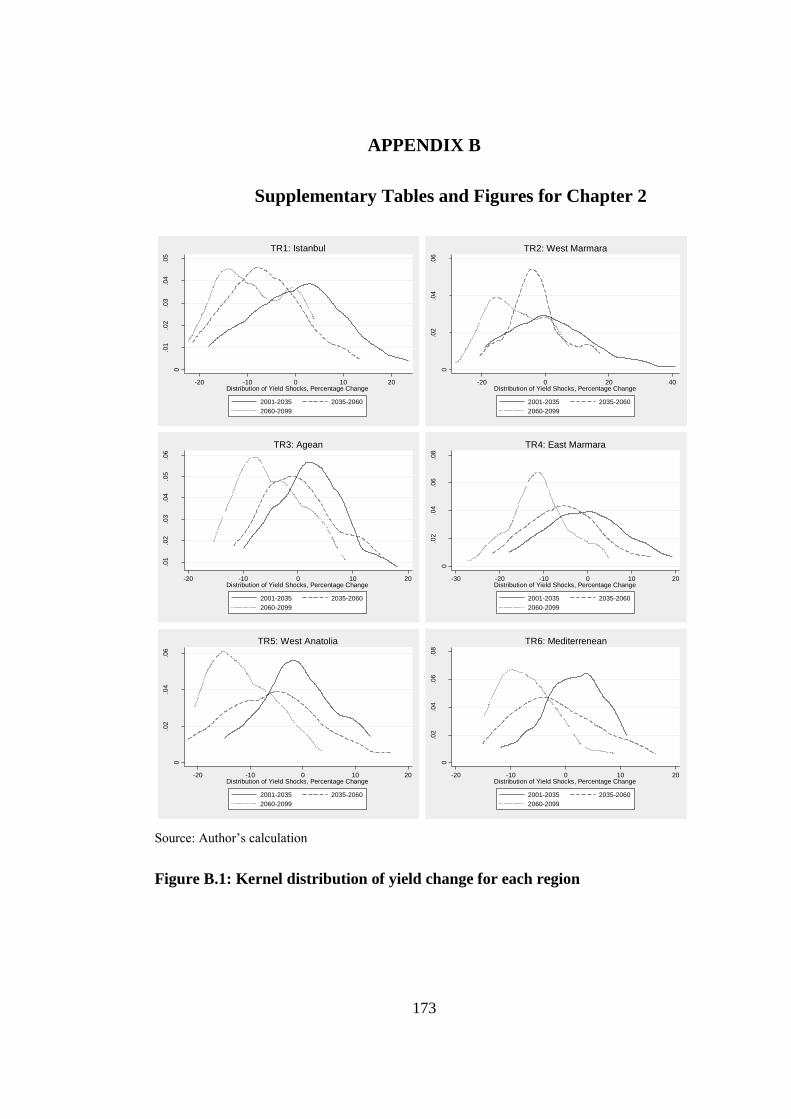
173

APPENDIX B

B. Supplementary Tables and Figures for Chapter 2

Source: Author’s calculation

Figure B.1: Kernel distribution of yield change for each region

0

.01

.02

.03

.04

.05

kd

en

sity d

tr1

-20 -10 0 10 20Distribution of Yield Shocks, Percentage Change

2001-2035 2035-2060

2060-2099

TR1: Istanbul

0

.02

.04

.06

kd

en

sity d

tr2

-20 0 20 40Distribution of Yield Shocks, Percentage Change

2001-2035 2035-2060

2060-2099

TR2: West Marmara

.01

.02

.03

.04

.05

.06

kd

en

sity d

tr3

-20 -10 0 10 20Distribution of Yield Shocks, Percentage Change

2001-2035 2035-2060

2060-2099

TR3: Agean0

.02

.04

.06

.08

kd

en

sity d

tr4

-30 -20 -10 0 10 20Distribution of Yield Shocks, Percentage Change

2001-2035 2035-2060

2060-2099

TR4: East Marmara

0

.02

.04

.06

kd

en

sity d

tr5

-20 -10 0 10 20Distribution of Yield Shocks, Percentage Change

2001-2035 2035-2060

2060-2099

TR5: West Anatolia

0

.02

.04

.06

.08

kd

en

sity d

tr6

-20 -10 0 10 20Distribution of Yield Shocks, Percentage Change

2001-2035 2035-2060

2060-2099

TR6: Mediterrenean

174

Source: Author’s calculation

Figure B.1: Kernel distribution of yield change for each region (continued)

0

.02

.04

.06

kd

en

sity d

tr7

-20 -10 0 10 20Distribution of Yield Shocks, Percentage Change

2001-2035 2035-2060

2060-2099

TR7: Central Anatolia

0.1

.2.3

kd

en

sity d

tr9

-6 -4 -2 0 2Distribution of Yield Shocks, Percentage Change

2001-2035 2035-2060

2060-2099

TR9: East Black Sea

0

.01

.02

.03

.04

.05

kd

en

sity d

tr8

-20 -10 0 10 20Distribution of Yield Shocks, Percentage Change

2001-2035 2035-2060

2060-2099

TR8: West Black Sea

0

.02

.04

.06

.08

kd

en

sity d

tra

-20 -10 0 10 20Distribution of Yield Shocks, Percentage Change

2001-2035 2035-2060

2060-2099

TRA: Northeast Anatolia

0

.02

.04

.06

.08

kd

en

sity d

trb

-20 -10 0 10Distribution of Yield Shocks, Percentage Change

2001-2035 2035-2060

2060-2099

TRB: Central East Anatolia

0

.02

.04

.06

.08

kd

en

sity d

trc

-20 -10 0 10 20Distribution of Yield Shocks, Percentage Change

2001-2035 2035-2060

2060-2099

TRC: Southeast Anatolia

175

Table B.1: Effects on selected aggregate variables of other sectors

BASE 2010-2035 2035-2060 2060-2100

Ma

nu

fac

turi

ng

Ma

rk. Prod. 142,478 0.01 -0.95 -2.62

Cons. 103,317 0.08 -1.52 -4.26

Prices 1.00 0.01 -0.60 -1.65

Em

pl. Labor 3,179 -0.01 -0.39 -1.06

Capital 73,739 0.05 -1.45 -4.01

Water 1,079 -0.02 0.32 0.90

Wa

ge Labor 21.29 0.06 -1.42 -3.93

Capital 1.00 0.00 0.00 0.00

Water 1.00 0.15 -2.27 -6.38

Tra

de Import 229,988 0.09 -2.14 -5.82

Export 135,216 -0.07 -1.46 -3.77

Deficit -94,772 0.31 -3.10 -8.74

Te

xti

le

Ma

rk. Prod. 35,046 0.04 -1.14 -3.14

Cons. 46,251 0.03 -0.53 -1.50

Prices 1.00 -0.01 -0.44 -1.19

Em

pl. Labor 1,657 0.03 -0.43 -1.17

Capital 22,141 0.06 -1.53 -4.24

Water 186.857 -0.01 0.21 0.64

Wa

ge Labor 7.68 0.03 -1.48 -4.11

Capital 1.00 0.00 0.00 0.00

Water 1.00 0.14 -2.25 -6.35

Tra

de Import 11,830 0.04 -0.90 -2.44

Export 32,308 0.06 -2.23 -6.03

Deficit 20,478 0.07 -3.00 -8.11

En

erg

y

Ma

rk. Prod. 14,031 0.06 -0.94 -2.68

Cons. 12,786 0.05 -0.75 -2.13

Prices 1.00 0.02 -0.37 -1.01

Em

pl. Labor 161 -0.05 -0.46 -1.26

Capital 10,800 0.08 -1.10 -3.13

Water 7.167 -0.01 0.40 1.12

Wa

ge Labor 20.09 0.16 -0.88 -2.58

Capital 1.00 0.00 0.00 0.00

Water 1.00 0.18 -1.91 -5.51

Tra

de Import 18.956 0.04 -1.17 -3.16

Export 101 0.00 -2.13 -5.68

Deficit 82 0.00 -2.35 -6.26

176

Table B.1: Effects on selected aggregate variables of other sectors (continued)

BASE 2010-2035 2035-2060 2060-2100

Pri

va

te S

erv

ices

Ma

rk. Prod. 429,450 0.09 -1.61 -4.51

Cons. 326,497 0.09 -1.85 -5.14

Prices 1.00 0.01 -0.45 -1.22

Em

pl.

Labor 10,012 0.03 -0.77 -2.22

Capital 308,817 0.12 -1.91 -5.36

Water 1,928 0.01 -0.15 -0.42

Wa

ge Labor 11.86 0.09 -1.55 -4.26

Capital 1.00 0.00 0.00 0.00

Water 1.00 0.17 -2.33 -6.54

Tra

de Import 34,029 0.14 -2.14 -5.86

Export 44,558 0.16 -2.59 -7.30

Deficit 10,529 0.21 -4.05 -6.00

Pu

bli

c S

erv

ice

s Ma

rk. Prod. 84,707 0.02 -1.07 -2.96

Cons. 19,477 0.04 -1.77 -4.85

Prices 1.00 0.08 -0.73 -2.07

Em

pl.

Labor 486 0.02 -0.94 -2.59

Capital 13,306 0.14 -1.71 -4.84

Water 573.957 0.01 -0.22 -0.59

Wa

ge Labor 145.59 0.13 -1.08 -3.07

Capital 1.00 0.00 0.00 0.00

Water 1.00 0.18 -1.97 -5.63

Note: Production and Consumption figures and quantity of water are quantities in terms of value added units,

i.e. units that make base prices 1. Labor is in thousand person. Rest of the base values are in million TL

Source: Author’s calculation

177

APPENDIX C

C. Supplementary Tables and Figures for Chapter 3

Table C.1: Statistics about yield and irrigation requirement changes

Crop Variable Statistics Period 1 Period 2 Period 3

Wheat

Irrigation Water Req.

Minimum -23.46 -31.28 -40.54 Mean -3.30 -3.92 1.06 Maximum 32.62 23.38 29.15 Standard Dev. 15.41 16.98 16.03

Yield

Minimum -9.14 -14.08 -30.51 Mean -2.15 -7.13 -17.55 Maximum 5.23 0.23 -7.53 Standard Dev. 4.16 3.51 5.68

Maize

Irrigation Water Req.

Minimum -20.33 -13.83 -23.28 Mean -3.30 -1.52 -5.02 Maximum 14.58 6.90 8.31 Standard Dev. 7.79 5.50 7.47

Yield

Minimum -19.32 -25.39 -54.83 Mean 2.45 -9.88 -29.73 Maximum 15.07 12.57 -8.62 Standard Dev. 9.40 8.46 13.15

Oilseeds

Irrigation Water Req.

Minimum -26.01 -20.52 -26.49 Mean -5.46 -6.62 -10.27 Maximum 12.06 5.42 7.33 Standard Dev. 9.52 8.38 7.59

Yield

Minimum -17.48 -22.71 -41.21 Mean -1.94 -15.44 -27.28 Maximum 27.26 -0.64 -11.00 Standard Dev. 13.20 5.15 7.37

Other Cereals

Irrigation Water Req.

Minimum -29.96 -28.24 -28.29 Mean -6.92 -3.01 1.33 Maximum 27.93 29.20 34.80 Standard Dev. 15.44 16.36 16.05

Minimum -0.47 -1.14 -4.94 Mean 0.82 -0.14 -2.32

Yield Maximum 1.93 1.32 -0.70 Standard Dev. 0.70 0.65 1.00

178

Table C.1: Statistics about yield and irrigation requirement (continued)

Crop Variable Statistics Period 1 Period 2 Period 3

Fruit

Irrigation Water Req.

Minimum -27.79 -30.95 -16.74

Mean -1.76 2.98 12.54

Maximum 24.80 33.26 40.26

Standard Dev. 12.65 16.28 13.53

Yield

Minimum -0.77 -2.77 -6.35

Mean 0.62 -1.32 -3.84

Maximum 2.58 -0.22 -0.87

Standard Dev. 0.84 0.62 1.35

Vegetable

Irrigation Water Req.

Minimum -36.37 -26.47 -19.87

Mean -4.44 1.09 10.41

Maximum 24.47 25.18 46.80

Standard Dev. 15.39 14.03 15.93

Yield

Minimum -2.86 -10.32 -15.61

Mean 5.35 -0.77 -7.33

Maximum 12.96 9.48 3.77

Standard Dev. 4.57 4.46 4.64

Other Field Crops

Irrigation Water Req.

Minimum -37.27 -31.86 -39.67

Mean -7.10 -3.61 0.73

Maximum 19.48 24.30 26.35

Standard Dev. 16.16 15.19 16.55

Yield

Minimum -6.88 -10.03 -21.35

Mean -0.25 -2.83 -10.02

Maximum 5.48 6.86 -0.55

Standard Dev. 3.45 3.59 5.22

Source: Crop water requirement model results

179

Wheat Maize

Oilseeds Other Cereals

Other Field Crops Fruit

Vegetable

Source: Model Results

Figure C.1: Change in yield and irrigation water requirement of selected crops

(percentage change from the base year)

180

Source: Model Results

Figure C.2: Sectoral value added and GDP growth under baseline (percentage

deviation from the base year)

Source: Model Results

Figure C.3: Change in CPI under baseline (percentage deviation from the base

year)

181

Source: Model Results

Figure C.4: Change in Imports and exports under the baseline (percentage

deviation from the base year)

Source: Model Results

Figure C.5: Labor Force growth in the baseline scenario.

182

Source: Model Results

Figure C.6: Growth path of factor supplies in the baseline scenario

Source: Model Results

Figure C.7: Standard deviation of change in imports to EU

183

Source: Model Results

Figure C.8: Change in imports to the other trading partners for the rest of the

sectors (percentage deviation from the baseline)

184

APPENDIX D

D. Supplementary Tables and Figures for Chapter 4

Source: Author’s adaptation from Brockmeier (1996)

Figure D.1: Detailed structure of GTAP model

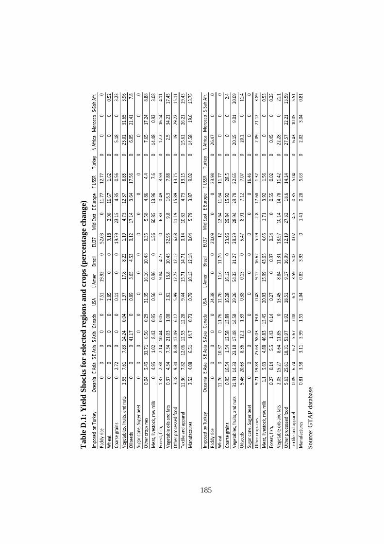
185

Tab

le D

.1:

Yie

ld S

hock

s fo

r se

lecte

d r

egio

ns

an

d c

rop

s (p

erce

nta

ge

cha

nge)

S

ou

rce:

GT

AP

dat

abas

e

186

So

urc

e: A

uth

ors

’ C

alcu

lati

on

fro

m I

MA

GE

an

d I

FP

RI

Dat

abas

es

Fig

ure

D.2

: Y

ield

Sh

ock

s fo

r se

lect

ed r

egio

ns

an

d c

rop

s (p

erce

nta

ge

chan

ge)

187

Source: Author’s adaptation from Brockmeier (1996)

Figure D.3: Most important trading partners of Turkey

Source: Model Results

Figure D.4: Distribution of decomposition of EV for USA

-97

9.0

82

,02

3.6

Alloc. ToT Inv-Sav

BASE

-49

1.3

82

76

.16

Alloc. ToT Inv-Sav

AGRI

-70

.49

13

.03

Alloc. ToT Inv-Sav

EU

-9,1

22

.98

93

.43

Alloc. ToT Inv-Sav

FULL

Graphs by sim

188

Source: Model Results

Figure D.5: Distribution of decomposition of EV for East Asia

Source: Model Results

Figure D.6: Distribution of decomposition of EV for Former USSR Region

-1,5

11.2

2,1

92.3

Alloc. ToT Inv-Sav

BASE

-191.4

224,3

66

Alloc. ToT Inv-Sav

AGRI

-99.2

950.3

1

Alloc. ToT Inv-Sav

EU-1

,857.6

39,1

68

Alloc. ToT Inv-Sav

FULL

Graphs by sim

-22

1.5

62

90

.49

Alloc. ToT Inv-Sav

BASE

-35

.72

50

0.4

7

Alloc. ToT Inv-Sav

AGRI

-10

0.8

8

3.4

8

Alloc. ToT Inv-Sav

EU

-1,5

28

.73

,09

8.3

Alloc. ToT Inv-Sav

FULL

Graphs by sim

189

Source: Model Results

Figure D.7: Distribution of decomposition of EV for Middle East

Source: Model Results

Figure D.8: Distribution of decomposition of EV for East Asia

-51

5.7

96

75

.22

Alloc. ToT Inv-Sav

BASE

-40

.84

53

5.4

3

Alloc. ToT Inv-Sav

AGRI

-13

0.6

5

5.4

3

Alloc. ToT Inv-Sav

EU

38

0.2

53

,39

0.7

Alloc. ToT Inv-Sav

FULL

Graphs by sim

-78

1.8

51

10

.06

Alloc. ToT Inv-Sav

BASE

-10

2.9

41

82

.86

Alloc. ToT Inv-Sav

AGRI

-48

.25

5.6

2

Alloc. ToT Inv-Sav

EU

99

.32

1,2

56

.8

Alloc. ToT Inv-Sav

FULL

Graphs by sim

190

Source: Model Results

Note: We present the average over all climate scenarios since variation is not significant

Figure D.9: Distribution allocative efficiency effects according to sectors for

Turkey (million USD)

Source: Model Results

Figure D.10: Distribution decomposition of terms of trade component of EV

(million USD)

-53.

275

275.

223

World Pri. Exp. Pri. Imp. Pri.

BASE

-270

10.6

75

World Pri.Exp. Pri. Imp. Pri.

AGRI

-7.8

8649

6.92

2

World Pri. Exp. Pri. Imp. Pri.

EU

-204

.914

909.

566

World Pri.Exp. Pri. Imp. Pri.

FULL

Graphs by Scenarios

191

So

urc

e: M

od

el R

esu

lts

Fig

ure

D.1

1:

Ch

an

ge

in i

mp

ort

an

d e

xp

ort

valu

es o

f agri

-food

sect

ors

in

Tu

rk

ey u

nd

er b

ase

lin

e (

per

cen

tage

chan

ge)

-42.534260.1423

Imp.

Val.

Exp

. V

al.

Ric

e

-39.066431.4969

Imp.

Val.

Exp

. V

al.

Whe

at

-41.587543.4875

Imp.

Val.

Exp

. V

al.

Gra

ins

-40.809274.1506

Imp.

Val.

Exp

. V

al.

Veg

& F

ruit

-89.627482.3163

Imp.

Val.

Exp

. V

al.

Oilse

ed

-28.776638.5243

Imp.

Val.

Exp

. V

al.

Sug

ar

bee

t/ca

ne

-70.024231.5726

Imp.

Val.

Exp

. V

al.

Oth

. C

rop

-53.972337.5144

Imp.

Val.

Exp

. V

al.

Liv

esto

ck

-8.543185.83248

Imp.

Val.

Exp

. V

al.

Veg

. O

il

-10.59025.45003

Imp.

Val.

Exp

. V

al.

Foo

d

Gra

ph

s b

y s

ecto

r

192

So

urc

e: M

od

el R

esu

lts

Fig

ure

D.1

2:

Dis

trib

uti

on

of

chan

ge

in i

mp

ort

an

d e

xp

ort

pri

ce o

f agri

-food

com

mod

itie

s in

Tu

rkey

un

der

EU

sce

nari

o (

per

cen

tag

e C

han

ge)

-.125428.13591

Imp

. P

ri.

Exp.

Pri.

Ric

e

-.17888.82611

Imp

. P

ri.

Exp.

Pri.

Whe

at

-.035997.841832

Imp

. P

ri.

Exp.

Pri.

Gra

ins

-.024899.972499

Imp

. P

ri.

Exp.

Pri.

Ve

g &

Fru

it

-.050698.815813

Imp

. P

ri.

Exp.

Pri.

Oilsee

d

-.11055.894953

Imp

. P

ri.

Exp.

Pri.

Su

ga

r be

et/

can

e

-.03751.59994

Imp

. P

ri.

Exp.

Pri.

Oth

. C

rop

-.005059.76997

Imp

. P

ri.

Exp.

Pri.

Liv

esto

ck

-.15198.056777

Imp

. P

ri.

Exp.

Pri.

Ve

g.

Oil

-.004214.59514

Imp

. P

ri.

Exp.

Pri.

Fo

od

Gra

ph

s b

y s

ecto

r

193

So

urc

e: M

od

el R

esu

lts

Fig

ure

D.1

3:

Dis

trib

uti

on

of

chan

ge

in i

mp

ort

an

d e

xp

ort

pri

ce o

f agri

-food

com

mod

itie

s in

Tu

rkey

un

der

AG

RI

scen

ari

o (

per

cen

tage

Ch

an

ge)

-2.707959.85154

Imp

. P

ri.

Exp.

Pri.

Ric

e

-1.584081.98353

Imp

. P

ri.

Exp.

Pri.

Whe

at

-1.5312.99067

Imp

. P

ri.

Exp.

Pri.

Gra

ins

-1.77647.29563

Imp

. P

ri.

Exp.

Pri.

Ve

g &

Fru

it-1.79965

1.19186

Imp

. P

ri.

Exp.

Pri.

Oilsee

d

-1.169451.05482

Imp

. P

ri.

Exp.

Pri.

Su

ga

r be

et/

can

e

-3.186721.21006

Imp

. P

ri.

Exp.

Pri.

Oth

. C

rop

-1.5559-.41108

Imp

. P

ri.

Exp.

Pri.

Liv

esto

ck

-.86708-.16885

Imp

. P

ri.

Exp.

Pri.

Ve

g.

Oil

-2.07648-.33084

Imp

. P

ri.

Exp.

Pri.

Fo

od

Gra

ph

s b

y s

ecto

r

194

So

urc

e: M

od

el R

esu

lts

Fig

ure

D.1

4:

Dis

trib

uti

on

of

chan

ge

in i

mp

ort

an

d e

xp

ort

pri

ce o

f agri

-food

com

mod

itie

s in

Tu

rkey

un

der

FU

LL

sce

nari

o

(per

cen

tage

chan

ge)

-.8511511.5969

Imp

. P

ri.

Exp.

Pri.

Ric

e

.599232.63083

Imp

. P

ri.

Exp.

Pri.

Whe

at

.118613.37775

Imp

. P

ri.

Exp.

Pri.

Gra

ins

-.697192.59587

Imp

. P

ri.

Exp.

Pri.

Ve

g &

Fru

it

-.221882.18446

Imp

. P

ri.

Exp.

Pri.

Oilsee

d

-2.256082.20309

Imp

. P

ri.

Exp.

Pri.

Su

ga

r be

et/

can

e

-2.380281.07457

Imp

. P

ri.

Exp.

Pri.

Oth

. C

rop

-.358923.02629

Imp

. P

ri.

Exp.

Pri.

Liv

esto

ck

-1.76772-.47599

Imp

. P

ri.

Exp.

Pri.

Ve

g.

Oil

-1.46377-.10505

Imp

. P

ri.

Exp.

Pri.

Fo

od

Gra

ph

s b

y s

ecto

r

195

Imp

ort

Pri

ces

un

der

AG

RI

Imp

ort

Pri

ces

un

der

FU

LL

sce

na

rio

So

urc

e: M

od

el R

esu

lts

Fig

ure

D.1

5:

Imp

ort

an

d e

xp

ort

pri

ces

un

der

tra

de

lib

erali

zati

on

sce

nari

os

(per

cen

tage

chan

ge)

Ex

po

rt P

rice

s u

nd

er A

GR

I

Ex

po

rt P

rice

s u

nd

er F

UL

L s

cen

ari

o

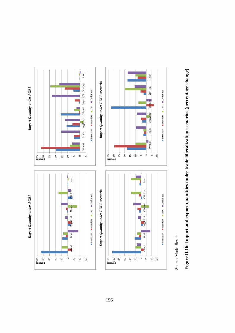
196

Imp

ort

Qu

an

tity

un

der

AG

RI

Imp

ort

Qu

an

tity

un

der

FU

LL

sce

na

rio

So

urc

e: M

od

el R

esu

lts

Fig

ure

D.1

6:

Imp

ort

an

d e

xp

ort

qu

an

titi

es u

nd

er t

rad

e li

ber

ali

zati

on

sce

nari

os

(per

cen

tage

chan

ge)

Ex

po

rt Q

uan

tity

un

der

AG

RI

Ex

po

rt Q

uan

tity

un

der

FU

LL

sce

na

rio

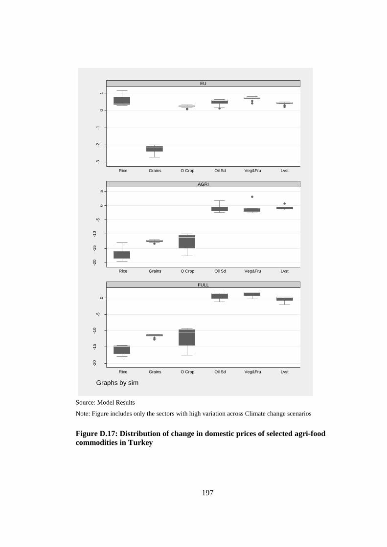
197

Source: Model Results

Note: Figure includes only the sectors with high variation across Climate change scenarios

Figure D.17: Distribution of change in domestic prices of selected agri-food

commodities in Turkey

-3-2

-10

1

Rice Grains O Crop Oil Sd Veg&Fru Lvst

EU

-20

-15

-10

-50

5

Rice Grains O Crop Oil Sd Veg&Fru Lvst

AGRI

-20

-15

-10

-50

Rice Grains O Crop Oil Sd Veg&Fru Lvst

FULL

Do

me

stic P

rice

Graphs by sim

198

Source: Model Results

Figure D.18: Distribution of change in production of agri-food commodities in

Turkey

010

20

30

Wht Gra VeFr OilSd Sug OCrp Lvst Extr V OilFoodManu Serv Tex Util

EU

-30

-20

-10

010

Wht Gra VeFr OilSd Sug OCrp Lvst Extr V OilFoodManu Serv Tex Util

AGRI

-20

020

40

Wht Gra VeFr OilSd Sug OCrp Lvst Extr V OilFoodManu Serv Tex Util

FULL

Pro

du

ctio

n

Graphs by Trade Simulations

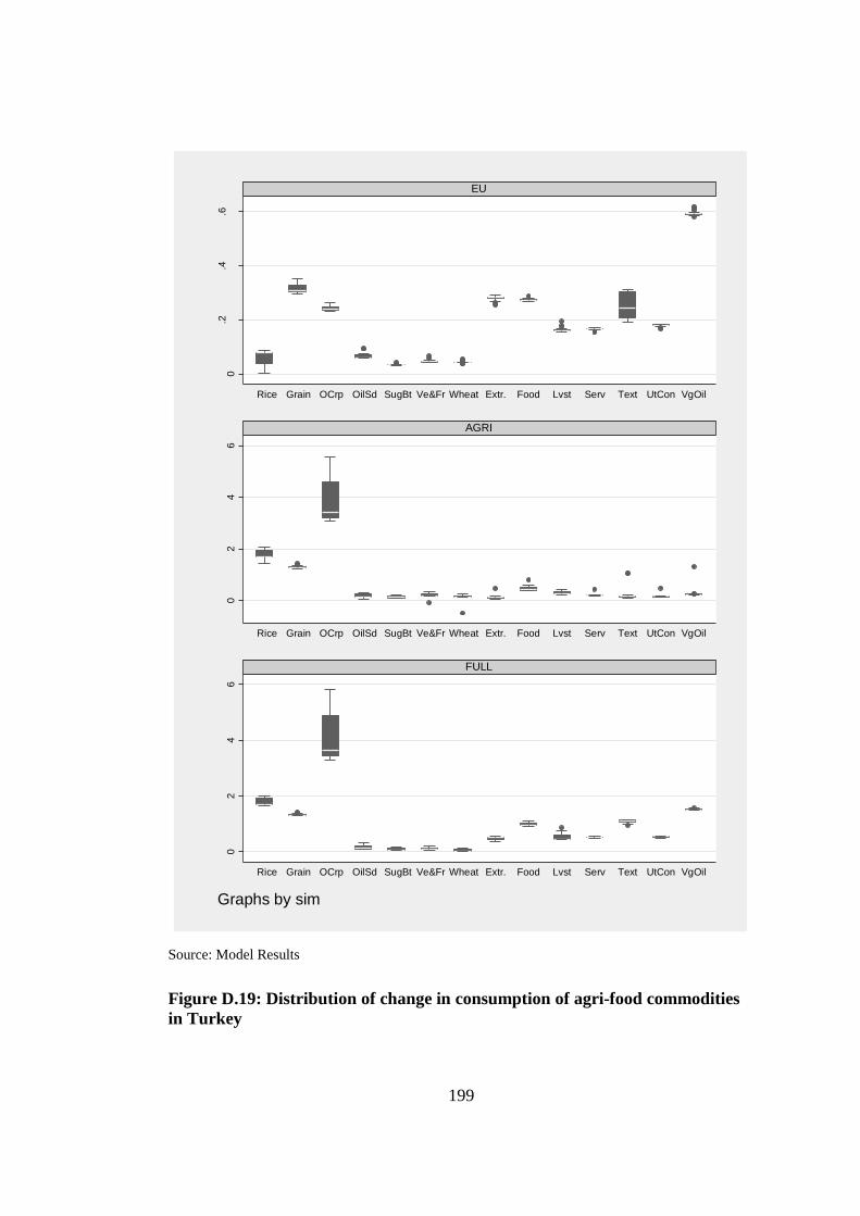
199

Source: Model Results

Figure D.19: Distribution of change in consumption of agri-food commodities

in Turkey

0.2

.4.6

Rice Grain OCrp OilSd SugBt Ve&Fr Wheat Extr. Food Lvst Serv Text UtCon VgOil

EU

02

46

Rice Grain OCrp OilSd SugBt Ve&Fr Wheat Extr. Food Lvst Serv Text UtCon VgOil

AGRI

02

46

Rice Grain OCrp OilSd SugBt Ve&Fr Wheat Extr. Food Lvst Serv Text UtCon VgOil

FULL

Pri

va

te C

on

su

mp

tio

n

Graphs by sim

200

Source: Model Results

Figure D.20: Average change in domestic prices under trade liberalization

scenarios

Source: Model Results

Figure D.21: Average change in production of agri-food commodities

201

APPENDIX E

E. TURKISH SUMMARY

Bölüm 1: Giriş

İklim değişikliği insanlığın, dünya üzerinde var olduğu günden bu yana, baş etmek

zorunda kaldığı en önemli sorunlardan birisi olmuştur. İnsan evriminin gerçekleştiği

2 milyon yıl boyunca iklim koşullarında meydana gelen döngüsel değişiklikler

önümüzdeki yüzyılda karşılaşmayı beklediğimiz değişikliklerden çok daha

şiddetliydi. Ancak türümüz, Afrika'da 500 bin yıl önce başlayıp, modern insanın

ortaya çıkmasına kadar devam eden büyük iklim dalgalanmalarına adapte olmak

konusunda oldukça başarılı oldu. Bugün de değişen iklim şartlarına adaptasyon

insanlığın kolektif olarak çözmek zorunda olduğu en büyük sorunlardan birisi

olarak uluslararası kamuoyunun gündemindedir.

İklim değişikliğine adaptasyon genel özellikleri itibariyle iktisadi bir problemdir.

Atalarımızın insan evriminin erken aşamalarında değişik iklimlere adaptasyon

konusunda geliştirdikleri en önemli yöntem "ekonomik" olmaktır. Homo sapiens

türü doğal kaynakları kullanmak konusunda en verimli organizmalardan birisi olma

özelliğine sahiptir. Sağlıklı bir insan vücudu biyosfer tarafından sağlanan hiç bir

şeyi israf etmez. Hayatta kalmak için bitkileri, hayvanları, madenleri ve hatta toprak

ve kayaları sonuna kadar kullanırız. Ne var ki bu hayatta kalma stratejisi tamamen

çevresinde var olanlara bağımlı bir tür ortaya çıkarmıştır. İnsanlık tarihi boyunca

türümüzün verdiği en temel mücadale hayatta kalmamızı sağlayacak kaynakları

güvence altına alma çabasıdır. Ancak bu çaba o kadar yoğun bir hale gelmiştir ki,

çabanın kendisi biyosferi değiştirerek –en azından iklim değişikliğini hızlandırarak-

esenliğimizi tehdit etmeye başlamıştır. Dolayısıyla insanlığın varlığını sürdürmek

konusunda başladığı noktaya döndüğü düşünülebilir. Yok olmak tehlikesini

202

atlatabilmek için "ekonomik olmanın" yeni yollarını bularak biyosferle etkileşim

stratejilerimizi geliştirmemiz gerekmektedir.

Bu tezin ana amacı iklim değişikliğini ve iklim değişikliğinin iktisadi faaliyetlerle

olan etkileşimini anlama çabasına katkıda bulunmakdır. Bu amaçla, tezi oluşturan

üç bölüm birbirlerinden bağımsız olarak tasarlanmakla birlikte, bir arada

değerlendirildiklerinde iklim değişikliği, tarım ve ticaret politkası arasındaki

bağlantıların bütüncül bir portresini çizmektedirler. Çalışmanın odağında Türkiye

olsa da, elde edilen sonuçlar çoğu gelişmekte olan ülke ve/veya bölgeyi kapsayacak

şekilde genelleştirilebilir. Çalışmamızda güncel teori ve verilere dayanan analitik

bir yaklaşım izlenmiştir. Statik yansıtımlar yerine, mümkün olan bütün gelecek

tasarımlarını betimlemeye çalışan stokastik bir yaklaşım takip edilmiştir. Yani,

iklim değişikliğinin fiziksel etkilerini değerlendirirken, sorunun özü itibariyle var

olan belirsizlikler de dikkate alınmıştır.

Bölüm 2: İklim Değişikliğinin Türkiye üzerindeki Etkilerinin Bütüncül bir

Yaklaşımla İncelenmesi

Hali hazırda su kaynakları önemli bir baskı altında olan Türkiye’de iklim

değişikliğinin etkilerinin belirgin olması kaçınılmazdır. Tezin ikinci bölümünün

amacı iklim değişikliklerinin ekonominin tamamı üzerindeki etkilerinin nicel

yöntemlerle ortaya konulmasıdır. Bu amaçla, 2008-2099 dönemi için hesaplanabilir

genel denge modeli ve bitki su gereksinimi modeli içeren bütünleşik bir yaklaşım

takip edilmiştir. İklim değişikliğinin etkileri en fazla tarım sektörünü etkileyeceği

için, olası etkilerin incelenmesinde tarımın ileri ve geri sektörel bağlantılarının

dikkate alınması gerekmektedir. Tezin ikinci bölümünde kullanılan hesaplanabilir

genel denge modeli tarım sektörü ve diğer sektörler arasındaki bağlantıları birinci

iktisadi bölge birimleri sınıflaması (İBBS-I) seviyesinde modellemektedir. Diğer

taraftan, 2010-2099 yılları arasında aylık olarak 81 ildeki 35 ürün için iklim

değişikliği kaynaklı verim ve sulama suyu gereksinimlerindeki değişimler bir bitki

su gereksinimi modeli ile hesaplanmıştır. Bitki su gereksinimi modelinin sonuçları

daha sonra hesaplanabilir genel denge modeline iklim şoku olarak sı-okulmuştur.

203

Bitki Su Gereksinimi Modeli ve Kullanılan Veri Seti

İklim değişikliğinin tarımsal üretimin teknik koşulları üzerindeki etkisi bitki-su

modelleri ile incelenebilir. Bu modeller yağış, sıcaklık ve rüzgâr hızı gibi ana iklim

değişkenleri ile ilgili tahminleri küresel dolaşım modellerinden alarak verim

değişikliklerini tahmin etmektedirler. Çalışmamızda iklim değişikliğinin bitkisel

üretim üzerindeki etkilerini ölçümlendirmek için Allen ve ark. (1998) tarafından

geliştirilen yöntemler takip edilmiştir. Bu yaklaşıma göre 81 ilde Aralık 2001 –

Aralık 2099 dönemi için aylık referans terleme-buharlaşmalar hesaplanmıştır.

Hesaplamalar için gerekli olan aylık yağış, sıcaklık ve rüzgar hızı verileri Dalfes ve

ark. (2010)’dan alınmıştır. Toprak ve bitkiye özel parametreler ise FAO (2011)’den

alınmıştır.

Allen ve ark. (1998)’de izlenen yöntem bitki terleme-buharlaşmasının referans

şartlarda (referans terleme-buharlaşma), standart şartlar altında (standart terleme-

buharlaşma) ve su stresi altında (stres altında terleme-buharlaşma) hesaplanmasına

dayanmaktadır. Referans terleme-buharlaşma standartlaştırılmış bir bitki örtüsünde

meydana gelen terleme-buharlaşmadır ve atmosferin buharlaştırma kapasitesini

gösterir. Referans terleme-buharlaşma sadece ışınım, hava durumu verileri

kullanılarak hesaplanmaktadır.

Standart terleme buharlaşma, veri iklim koşullarında belirli bir bitki türü için

optimum su yönetimi ve çevresel koşullar altında en yüksek verim elde edilen

terleme-buharlaşma miktarıdır. Dolayısıyla referans ve standart terleme-

buharlaşmalar arasındaki fark bitkiye özgü ”terleme direnci, bitki boyu, bitki

sertliği, yansıtım, yüzey kaplama ve bitki kök derinliği” (Allen ve ark., 1998) gibi

karakteristikler arasındaki farklar tarafından belirlenmektedir. Bu farklar değişik

bitki karakteristikleri kullanılarak hesaplanan ve standart bitki katsayısı olarak ifade

edilen bir parametre ile ifade edilir.

Su stresi altındaki terleme-buharlaşma, yağış veya sulama eksikliği nedeniyle

topraktaki su miktarının düşük olması nedeniyle ortaya çıkan terleme-

buharlaşmadır. Standart ve su stresi altındaki terleme-buharlaşma arasındaki fark

204

erişilebilir su miktarı, toprak karakteristikleri, yağış miktarı ve bitki özellikleri ile

hesaplanan su stresi katsayısı tarafından ifade edilmektir.

Çalışmamızda göreceli olarak entegre olmuş bir dünya ve hızlı ekonomik büyümeye

sahip bir gelecek öngörüsünde bulunan IPCC B1 senaryosu altında bitki sulama

gereksinimleri ve verimleri hesaplanmıştır. IPCC B1 senaryosu 2050 yılına kadar

dünya nüfusunun 9 Milyar kişiye ulaşacağını ve ondan sonra yavaş yavaş

düşeceğini varsaymaktadır. Bu senaryoda iktisadi büyüme hizmetler ve iletişim

sektörlerine odaklı seyrederken, iktisadi sürdürülebilirlik önemlidir.

Referans ve su stresi altındaki terleme-buharlaşma katsayıları Dalfes ve ark. (2011)

tarafından hesaplanan rüzgar hızları, yağış ve ortalama sıcaklıklar kullanılarak her

ilde ve 2001-2099 yılları için aylık olarak hesaplanmıştır. En düşük ve en yüksek

sıcaklıkların yayılımı, kritik boşalma, bitki boyu, başlangıç standart bitki katsayısı

değerleri, bitki ekim tarihleri, bitki gelişim süreleri, kök derinliği, verim yanıt

katsayıları ve toprak parametreleri Allen ve ark. (1998)’den alınmıştır.

Bitki su gereksinimi modelinin sonuçları literatürde yapılmış olan benzer

çalışmaların bulgularlıyla tutarlıdır. Model sonuçlarına göre, Türkiye’de tarımsal

üretimin teknik koşulları ortalamada kötüleşmektedir. İklim değişikliğinin olumsuz

etkileri 2060’dan sonra belirgin bir hal almaktadır. Model sonuçları ayrıca iklim

değişikliğinin etkilerinin ülke genelinde homojen olmayacağını ve mevsimler

arasında önemli farklılıklar göstereceğini de ortaya koymaktadır. Sonuçlar

incelendiğinde, iklim değişikliğinin tarımsal üretimin teknik koşulları üzerindeki

etkilerinin özellikleri açısından önümüzdeki yüzyılın üç döneme ayrılabileceği

görülmektedir. 2010-2035 yılları arasındaki birinci dönemde özellikle batı

bölgelerinde, ortalama yağışlarda %20’ye varan artışlar gözlemlenmektedir. En

önemli artış kış (Ocak-Mart) aylarında olacaktır. Diğer mevsimlerde, ortalama

yağışlar doğu bölgelerinde azalırken batı bölgelerinde yüksek seyretmektedir. 2036-

2060 yıllarını kapsayan ikinci dönemde kış aylarında yağış desenleri pek fazla

değişmezken, yılın geri kalan dönemlerinde belirgin bir şekilde değişmektedir.

2061-2099 yıllarını kapsayan üçüncü dönemde ise kuzey bölgelerinde kışın

205

gözlemlenen yüksek ortalama yağış miktarları korunurken, ülkenin geri kalanında

ortalama yağışlarda ciddi azalmalar meydana gelecektir.

Yağış ve sulama gereksinimlerindeki değişikliklerin verim ve sulama gereksinimleri

üzerindeki etkisi hem bölge hem de bitki türüne göre değişiklik göstermektedir. Bu

etkiler verim ve sulama gereksinimlerindeki değişiklikler bakımından dört grup

senaryo altında incelenebilir. Verim ve sulama gereksinimlerinin eş zamanlı olarak

arttığı durumlar birinci grubu oluşturmaktadır. Bu durum genellikle birinci

dönemde izlenmekte, ikinci ve üçüncü dönemlerde ise istisnai olarak ortaya

çıkmaktadır. Bu guruptaki bitki üretim faaliyetleri, daha yüksek verimler için daha

fazla sulama gerektireceğinden, uygun sulama yatırımları ile bu durumların

gözlendiği bölgelerin söz konusu ürünlerin yetiştirilmesinde bir avantaj sahibi

olması mümkündür. Verimler yükselirken, sulama gereksinimlerinin düştüğü

durumlar ikinci grubu oluşturmaktadır. Dolayısıyla bu gruptaki üretim faaliyetleri,

bu durumun gözlendiği bölgelerde tarımsal üretimde baskın hale gelecektir. Bu

durum genellikle birinci dönemde gözlemlenmektedir. Verimlerin ve sulama

gereksinimlerinin aynı anda düştüğü durumlar üçüncü grubu oluşturmaktadır. Bu

durum, ülke genelinde ve bütün dönemlerde en sık olarak gözlemlenen durumdur.

Verimler düşerken sulama gereksinimlerinin arttığı durumlar son grubu

oluşturmaktadır. Bu guruptaki üretim faaliyetlerinin teknik koşulları önemli ölçüde

kötüleşmektedir. Bu durum genellikle ikinci ve üçüncü dönemde

gözlemlenmektedir.

Sonuç olarak bulgularımız 2030’lu yıllara kadar tarımsal üretimin önemli bir

kısmının iklim değişikliğinin etkilerinden olumlu yönde etkileneceğini

göstermektedir. Ne var ki, bunda sonra ve özellikle 2060’lı yıllardan sonra hemen

hemen bütün ürünler için üretim koşulları belirgin bir şekilde kötüleşecektir.

Tahıllar gibi geleneksel ürünler iklim değişikliğinden oldukça olumsuz bir şekilde

etkilenecektir. Meyve üretimi üzerindeki etkiler de özellikle son dönemde oldukça

olumsuzdur. Bu sonuçlara göre Türkiye’de sulama yatırımı planlaması yapılırken

iklim değişikliğinin heterojen etkilerinin dikkate alınması çok önemlidir. Özellikle

birinci ve ikinci dönemlerde, verimlerin düşmesinin önlenmesi önemli ölçüde

206

sulama altyapısının geliştirilmesi ile mümkün olacaktır. Uzun vadede ise kuraklığa

dayanıklı türlerin geliştirilmesi ve yaygınlaştırılması tek çözüm olarak görünmekte

ve bu sebeple tarımsal Ar-Ge çalışmalarının desteklenmesinin önemini ortaya

koymaktadır.

Statik HGD Modeli ve Kullanılan Veri Seti

Bu bölümde geliştirilen Walrasyan hesaplanabilir genel denge modeli, ekonomiyi

12 IBBS-1 bölgesinde 7 sektör için üretim yapan 7 üretim faaliyetine ayırmaktadır.

Üretim faaliyetleri tarım, gıda üretimi, tekstil, diğer sanayi üretimi, enerji, özel

hizmetler ve kamu hizmetleri sektörleridir. Ekonomideki her sektör diğer

sektörlerden sağlanan ara malı girdileriyle birlikte üretim faktörü olarak işgücü,

sermaye, susuz toprak, sulu toprak, tarımsal sulama suyu ve sınai su kullanarak

üretim yapan bir üretim faaliyeti ile temsil edilmektedir. Üretim fonksiyonunun

kademeli bir yapısı vardır. Birinci kademede sulama suyu ile sulu toprak Leontief

tipi bir üretim fonksiyonuna girerek sulama suyu-sulu toprak bileşik faktörünü

oluşturmaktadır. Bu şekilde bu iki faktör arasındaki tamamlayıcılık ilişkisi modele

dâhil edilmektedir. Bu bileşik faktör ikinci kademede diğer üretim faktörleri ile

birlikte sabit ikame esneklikli bir üretim fonksiyonuna girerek bir çeşit bileşik

üretim faktörü üretmektedir. Diğer taraftan, yine ikinci kademede, ara malı girdileri

Leontief tipi bir üretim fonksiyonunda bileşik girdiye dönüştürülmektedir. Üçüncü

kademede ise bileşik üretim faktörü sabit ikame esneklikli bir üretim faktörüne

girerek katma değer cinsinden nihai ürünü oluşturmaktadır.

Üretim sürecinde üretilen ürünler yurt içi piyasalara ara malı ve nihai mal olarak ve

aynı zamanda uluslararası piyasalara ihracat ürünü olarak arz edilmektedir. Üretim

faaliyetleri devlete üretim vergisi ödemekte ve devletten destek almaktadırlar.

Sermaye tarafından yaratılan katma değer gelir olarak firmalara ödenmektedir.

Firmalar devletten ve yurt dışından gelir transferleri almaktadırlar. Firma gelirleri,

hanehalkına sermaye geliri, devlete kurumlar vergisi ve yurt dışına sermaye

transferi olarak aktarılmaktadır.

207

Hanehalkları işgücü, toprak ve su tarafından yaratılan katma değeri gelir olarak

doğrudan almaktadırlar. Hanehalklarına da devletten ve yurt dışından gelir transferi

yapılmaktadır. Hanehalkı bu gelirleri tüketim harcamaları yapmak, gelir vergisi

ödemek ve tasarruf yapmak için kullanmaktadır. Tüketim doğrusal harcama sistemi

yöntemi ile modellenmiştir. Buna göre hanehalkı geçimlik tüketim seviyesinin

üzerinde tükettiği ürün miktarı kadar fayda elde etmektedir.

Dinlence zamanı da fayda fonksiyonuna dâhil edilmiştir. Kalibrasyon ile ilgili

güçlükleri aşmak için işgücüne dâhil olan işsiz nüfusun hâlihazırda iş aramayan

kısmını dinlence zamanının bir göstergesi olduğu varsayılmıştır. İşgücüne dâhil

olmayan nüfus ise (öğrenciler, ev hanımları, emekli kişiler vs…) geçimlik dinlence

seviyesi olarak kabul edilmiştir. Bu yaklaşım, hanehalkının işgücü arzı davranışını

modelleme imkânı tanısa da mevcut tüketim sisteminde geçimlik dinlence

miktarının içsel hale getirilmesi mümkün olmadığı için işgücüne katılım hala dışsal

olarak ele alınmak zorundadır. Ne var ki, işgücüne katılımın sabit dışsal bir

değişken olarak kalmasının önüne geçmek için iş gücüne katılımın bir “hareket

kuralı” çerçevesinde belirlendiği varsayımı yapılmıştır. Buna göre, işgücüne

katılım reel ücretlerdeki değişimin bir fonksiyonudur. Reel ücretler arttıkça

işgücüne katılım da artmaktadır.

Hanehalkının tasarruf davranışı model kapama kuralları ile belirlenmektedir. Makro

düzeyde tasarrufların yatırımlar tarafından belirlendiği ve toplam absorpsiyondaki

düzeltmelerin tüm ürünlere aynı ölçüde yansıdığı varsayılmıştır. Dolayısıyla,

yatırımların absorpsiyon içindeki payı sabit olup iktisadi birimlerin tasarruf oranları

yatırımları finanse edecek şekilde eşit oranda ölçeklendirilmektedir.

Devlet ile ilgili herhangi bir davranışsal varsayım yapılmamıştır. Devlet vergi

toplamakta ve yurt dışından gelir transferleri almaktadır. Devlet gelirleri kamu

tüketimi, kamu tasarrufu, yurt içindeki kurumlar ve kişiler ile yurt dışına gelir

transferi ödemeleri yapmak için kullanılmaktadır. Toplam devlet harcamalarının

toplam absorpsiyon içindeki payı sabittir. Devlet tasarruflarının esnek, vergi

oranlarının ise sabit olduğu varsayılmıştır.

208

Dış âlemler hesabı Türkiye’ye ithal malları arz edip, Türkiye’den ihracat mallarını

talep etmektedir. Ayrıca yurtiçi kurumlara gelir transferi ödemeleri yapmakta ve

onlardan gelir transferi ödemeleri almakta ve Türkiye’ye yatırım yapmaktadır.

İthalat, Armington yaklaşımı ile modellenmiştir ve sabit esneklikli bir dönüşüm

fonksiyonu tarafından yönetilmektedir. Buna göre, ithal edilen ürünler yurt içinde

üretilen ürünlerle tam ikame malları değildir ve ithalat talebi ile yerli mal talebi bir

ikame esnekliği tarafından belirlenmektedir. Dış âlem tasarrufu her zaman cari açığı

finanse edecek şekilde ithalat ve ihracat arasındaki farka eşittir. Yurt içindeki

kurumlara ve bu kurumlardan yapılan gelir transferlerinin bu kurumların gelirleri

içindeki payı sabittir.

Çalışmamızda kullanılan sosyal hesaplar matrisi Yiğiteli (2010) tarafından

hesaplanmış olan toplulaştırılmış sosyal hesaplar matrisine dayanmaktadır. Yiğiteli

(2010) sosyal hesaplar matrisi 2008 yılı için gelir gruplarına göre 5 çeşit

hanehalkının tüketimi için kayıt dışı işgücü, kayıtlı işgücü, toprak ve sermaye

kullanarak üretim yapan 49 sektör içermektedir. Bu bölümün amaçları

doğrultusunda bu sosyal hesaplar matrisi yedi sektör ve bir hanehalkı içerecek

şekilde toplulaştırılmış ve daha sonra 12 IBBS-1 bölgesine ayrılmıştır. Girdi çıktı

tablosunun bölgeselleştirilmesi Artırılmış Flegg Mekânsal Orantılama (Augmented

Flegg Location Quotiens – AFLQ) yöntemi ile yapılmıştır. sosyal hesaplar

matrisinin diğer satır ve sütunları belirli varsayımlar altında çeşitli veri setleri

kullanılarak yapılmıştır.

Türkiye, coğrafi ve sosyal özellikleri bakımından birinden çok farklı bölgelere

sahiptir. Bu farklılıklar üretim ve tüketim desenlerindeki farklılıklar olarak

ekonomiye de yansımaktadır. Farklı bölgesel yapılar karmaşık bir ekonomik

ilişkiler ağı ortaya çıkarmaktadır. İklim değişikliğinin muhtemel etkilerinin tam

olarak anlaşılabilmesi bu karmaşık ilişkiler ağının da dikkate alınması

gerekmektedir.

Tezin ikinci bölümünün amaçlarına uygun olarak bitki su gereksinimi modelinden

elde edilen verim ve sulama gereksinimleri değişimleri hesaplanabilir genel denge

209

modeline iklim şokları olarak sokulmuştur. Verimlerdeki değişim, tarım sektöründe

toplam faktör verimliliği şoku olarak; sulama gereksinimlerindeki değişim ise

üretim fonksiyonunun sulanan toprak-sulama suyu kademesindeki Leontieff

katsayısının, yani birim alan için gereken su miktarının, artışı şeklinde modele dâhil

edilmiştir. Benzetimler 2008-2099 yılları için karşılaştırmalı statik deneyler

şeklinde yapılmaktadır.

Bulgular

Benzetim sonuçlarına göre iklim değişikliğinın sebep olduğu verim ve sulama

gereksinimlerindeki değişimler üretim deseni ve göreceli fiyatları sert bir biçimde

değiştirecektir. Bunun sonucunda tarım ve gıda üretimi önemli ölçüde azalacak, bu

ürünlerin fiyatları ise buna paralel olarak ciddi oranda yükselecektir. Kıyı bölgeleri

iklim değişikliğinin ekonomik etkilerinden 2060’lı yıllara kadar daha az etkilenecek

ancak bundan sonra bu etkiler önemli ölçüde kötüleşecektir. Bütün dönemlerde

göreceli olarak daha az sulu üretim yapan bölgeler üzerinde iklim değişikliğinin

etkileri daha az olumsuzdur ve bu, sulama gereksinimlerindeki artışın verimlerdeki

düşüşler kadar önemli olduğunu göstermektedir. Refah göstergelerinde de benzer

bir desen gözlemlenmektedir. Doğu bölgelerindeki Hanehalkları iklim

değişikliğinden daha az etkilenmektedirler.

2035 yılından sonra dış dış ticaret hacmi ciddi oranda düşmektedir. Sanayi dışındaki

bütün sektörlerde dış ticaret dengesi kötüleşmekte ancak toplam cari açık

azalmaktadır. Tarım ve gıda sektörlerinde ithalata bağımlılık artmakta ve bu da orta

ve uzun vadeli politika tasarımlarında gıda güvencesi ile ilgili politikaların önemini

göstermektedir.

Birinci bölümde elde edilen bulgular literatürdeki ulusal veya küresel düzeyde

yapılmış olan diğer çalışmaların bulguları ile de uyumludur. İklim değişikliğinin

iktisadi etkileri bölgelere göre farklılıklar göstermektedir. Örneğin, iklim değişikliği

bazı bölgelerde refah kaybına neden olmamaktadır. Bunun anlamı iklim değişikliği

politikasının tasarlanmasında bölgeler arasındaki farklılıkların dikkate alınması

gerektiğidir. Pek çok çalışma tarafından öngörüldüğü gibi olumsuz etkiler 2030’lu

210

yıllardan sonra özellikle aşırı olayların daha sık olarak yaşanması yoluyla daha

belirgin hale gelmektedir. En kötümser durumda gayri safi yurt içi hasıla (GSYİH)

kayıpları %10’a kadar yükselmektedir.

Bölüm 3: İklim Değişikliği, Tarım ve Ticari Serbestleşme: Türkiye için

Dinamik HGD Analizi

Tezin üçüncü bölümünde dinamik bir hesaplanabilir genel denge modeli

geliştirilmiştir. Bu model ulusal düzeydedir ve tüm Türkiye’yi tek bir bölge olarak

ele almaktadır. Modelde tarım sektörü daha detaylı olarak inceleme yapmak

amacıyla alt sektörlere ayrıştırılmıştır. Ayrıca modelin dış âlemler hesabı beş ticaret

ortağını içerecek şekilde yeniden tasarlanmıştır.

Geliştirilen bu modelle iklim değişikliği ve ticari serbestleşme benzetimleri

yapılarak dış ticareti serbestleştirmenin iklim değişikliğinin olumsuz etkilerini

hafifletip hafifletmediği incelenmiştir. Kullanılan iklim değişikliği senaryosu,

birinci bölümde kullanılan senaryonun detaylı bir versiyonudur. Dış ticaret

serbestleşmesi senaryosu ise Türkiye’nin AB’ne uyguladığı gümrük vergilerinin

kaldırılması şeklinde tasarlanmıştır. İklim değişikliği bütün dünyayı etkileyecek bir

olgu olduğu için küresel çapta tarımsal fiyatların değişmesi kaçınılmazdır ve bu, dış

ticaret serbestleşmesinin olası etkileri üzerinde önemli farklılıklar yaratabilir. Ne

var ki tarım fiyatlarındaki bu olası değişimin yönü ve büyüklüğü bilinmemektedir.

Tarım fiyatlarındaki belirsizliği analize dâhil etmek için dünya tarım fiyatlarının

normal bir dağılımdan geldiğini ve bu dağılımın ortalamasının ve standart

sapmasının iklim değişikliği tarafından değiştirileceği varsayılmıştır. Kötüleşen

ortalama şartları ve artan iklim riskini betimlemek için dünya fiyatlarının

dağılımının ortalamasının artacağı, ancak standart sapmasının aynı kalacağını

varsayılmıştır. Bu varsayım altında elde edilen model sonuçları iklim değişikliğinin

dünya fiyatları üzerindeki etkisinin ne kadar önemli olduğuna dair sonuçlar üretmek

için kullanılmıştır.

Model ve Kullanılan Veri Seti

211

Bu bölümün amaçlarına uygun olarak, ikinci bölümde geliştirilmiş olan statik

hesaplanabilir genel denge modeli Thurlow’un (2004) yöntemi izlenerek

özyinelemeli dinamik hale getirilmiştir. Dinamik süreç sermaye birikimi,

üretkenlik, nüfus ve işgücüne katılımdaki büyüme süreçleri üzerinden işlemektedir.

Dinamik hesaplanabilir genel denge modeli tarafından kullanılan sosyal hesaplar

matrisi, ikinci bölümde kullanılan sosyal hesaplar matrisinin üzerinde yapılan üç

değişiklikle elde edilmiştir. Öncelikle, bölüm 2’de kullanılan sosyal hesaplar matrisi

bölgeler üzerinde toplulaştırılarak ulusal sosyal hesaplar matrisi elde edilmiştir.

İkinci olarak, daha detaylı bir inceleme yapılabilmesi amacı ile tarım sektörü 13 alt

sektöre ayrılmıştır. Bu alt sektörler: buğday, mısır, pirinç, diğer tahıllar, yağlı

tohumlar, şeker pancarı, diğer tarla bitkileri, meyve, sebze süt ürünleri, et, diğer

hayvancılık faaliyetleri ve son olarak diğer tarımsal faaliyetlerdir. Tarım dışı

sektörler birinci bölümdeki halleri ile kalmıştır: Gıda üretimi, tekstil, enerji, diğer

snayi üretimi, özel hizmetler ve kamu hizmetleri. Son olarak, sosyal hesaplar

matrisinin dış âlemler hesabı 5 bölgeye ayrıştırılmıştır. Bu bölgeler: Avrupa Birliği

ülkeleri, diğer Avrupa ülkeleri, Kuzey Amerika, Orta Doğu ve Kuzey Afrika ile

Dünyanın geri kalanıdır.

İklim değişikliği senaryolarının altında AB ile Türkiye arasında meydana gelecek

bir ticari serbestleşmenin etkilerini incelemek için 2008-2099 yılları arasında üç

senaryo benzetimi yapılmıştır. Öncelikle ekonominin uzun vadeli ortalama büyüme

desenini taklit eden bir referans senaryo oluşturulmuştur. Referans senaryonun

sonuçları diğer senaryolar için kıyas noktası olarak kullanılmıştır. İklim değişikliği

senaryosunda verim ve sulama suyu gereksinimlerindeki değişimler referans

senaryodaki varsayımların üzerine iklim şoku olarak eklenmektedir. Son olarak

Türkiye’nin tek taraflı olarak ithalat vergilerini kaldırdığı durumun benzetimi

yapılmıştır. İklim değişikliği ve ithalat vergilerinin tek taraflı kaldırılması

senaryolarının benzetimi 48 farklı dünya fiyat değişikliği varsayımı altında

yapılmıştır. Varsayılan dünya fiyat değişimi serileri Gaussyan Dördülleme yöntemi

kullanılarak dünya fiyatlarının geçmiş yıllarda gözlemlenen istatistiksel özellikleri

kullanılarak hesaplanmıştır.

212

Benzetim sonuçlarına göre iklim değişikliği %3.5’e varan GSYİH kayıplarına

neden olabilecektir. GSYİH’deki kayıpların ana etmenleri özel tüketimlerdeki

düşüşler ve ithalatta meydana gelen belirgin artışlardır.

İthalat vergilerinin kaldırılması iklim değişikliğinin Türkiye ekonomisi üzerindeki

bu olumsuz etkilerini kısıtlı bir şekilde azaltmaktadır. Ticari serbestleşmenin

sağladığı refah artışı, iklim değişikliğinin sebep olduğu refah kayıpları ile

kıyaslandığında oldukça küçük kalmaktadır. Ne var ki, ticari serbestleşmenin refah

arttırıcı etkisi, iklim değişikliğinin etkileri kötüleştikçe – özellikle 2060’lı yıllardan

sonra – artmaktadır. Bunun sebebi, dış ticaret serbestleşmesinin iktisadi birimlere

hem üretim hem tüketim sürecinde daha fazla ikame olanağı vermesidir. Dış ticaret

serbestleşmesi altında ekonominin temel intibak mekanizması üretimde ara malı

girdilerinin faktörlerle ve tüketimde ithal malların yerli mallarla ikame edilmesidir.

Bunun sonucunda sektörel düzeyde önemli değişiklikler gözlenmektedir. Buğday,

pirinç ve diğer tahıllar dış ticaret serbestleşmesinden en fazla etkilenen sektörler

olarak ön plana çıkmaktadır. İklim değişikliği önemli ölçüde verimlilik kaybına

sebep olduğu için bu ürünler hem yerel hem de ithal alternatifleri karşısındaki

rekabet güçlerini önemli ölçüde kaybetmektedirler. Üretimleri, ihracatları ve

fiyatları önemli ölçüde gerilediği için bu ürünler ithal mallarla en fazla ikame edilen

ürünlerdir. Diğer taraftan mısır, yağlı tohumlar, meyve ve işlenmiş gıda dış ticaret

serbestleşmesinden olumlu etkilenmektedirler. Bu ürünlerin üretim ve ihracatları

artmakta fiyatları düşmekte ve ithalatları çok fazla değişmemektedir. İklim

değişikliği şoklarından sonra daha verimli hale geldikleri için üretim faktörlerinin

bu sektörlerdeki istihdamında artış gözlenmektedir.

AB ülkelerinden yapılan ithalatta belirgin artışlar meydana gelmekte ve bu da iç

piyasadaki fiyatların önemli ölçüde düşmesine sebep olmaktadır. Bunun neticesinde

tarımsal üretim düşmektedir. Yerel fiyatlarda meydan gelen düşüş, dış ticaret

yapılan diğer bölgelere uygulanan ithalat vergilerinden düşük olduğu için diğer

bölgelerden yapılan ithalatta düşüşler görülmektedir. Bunun neticesinde toplam

ithalat azalmaktadır. Dolayısıyla AB ile yapılan dış ticaret serbestleşmesi dış ticaret

kayması yaratmaktadır.

213

Bu bölümde sunulan analiz pek çok yönden geliştirilebilir. Örneğin, diğer ülkeler de

iklim değişikliğinden etkilenecekleri için Türk ihracat mallarına talepleri ve

Türkiye’ye yaptıkları ithalat arzı da bundan etkilenecektir. Böyle bir değişiklik

iklim değişikliğinin ve dış ticarette serbestleşmenin Türkiye üzerindeki etkilerini

değiştirebilir. İkinci olarak AB ile tek taraflı yapılacak olan bir dış ticaret

serbestleşmesi Türkiye’nin dış ticaret politikasındaki tek seçenek değildir. Diğer

bölge ve ülkelerle yapılacak olan bir dış ticaret anlaşmasının etkileri çok daha

büyük olabilir. Son olarak, bu bölümde tek bir küresel dolaşım modelinin sonuçları

kullanılmıştır. Farklı küresel dolaşım modellerinin kullanılması iklim değişikliğinin

olası sonuçları konusunda daha bütüncül bir analiz yapılmasına olanak tanıyabilir.

Bölüm 4: İklim Değişikliğine Küresel bir Adaptasyon Aracı olarak Dış ticaret

Politikaları

Tezin dördüncü bölümünde, iklim değişikliğinin küresel ekonomi üzerindeki etkisi

incelenmiş ve değişik ticari serbestleşme politikalarının bu etkilerle etkileşimi

incelenmiştir. Bu amaçla dördüncü bölümde GTAP modeli kullanılmıştır. GTAP

literatürde dış ticaret politikası analizi için sıkça kullanılan detaylı bir küresel

hesaplanabilir genel denge modelidir. GTAP’in tezin dördüncü bölümde kullanılan

versiyonunda 16 bölge ve 15 aktivite vardır ve GTAP 7 veri tabanını

kullanmaktadır. Benzetimler konusunda tezin dördüncü bölümde de üçüncü

bölümünde izlenen yaklaşım izlenmiştir. Modele 25 farklı iklim yansıtımından

gelen iklim şokları sokularak referans senaryolar oluşturulmuş, daha sonra dış

ticaret serbestleşmesi benzetimlerinin sonuçları bu referans senaryoların sonuçları

ile kıyaslanmıştır.

Kullanılan Model ve Veri Seti

GTAP, hanehalkaları, üreticiler ve kamu sektörünün davranışlarını genel denge

teorisinin standart varsayımlarını takip ederek modelleyen çok bölgeli, küresel ve

statik bir HGD modelidir. Hanehalkları fayda maksimizasyonu yapan ve ekonomide

üretilen bütün geliri alan ekonomik birimlerdir. Bu gelir, özel tüketim ve

tasarruflara Cobb-Douglas fayda fonksiyonuna göre harcanmaktadır. Yani hane

214

halkının tasarruf kararı tüketim kararı ile eşzamanlı olarak alınmaktadır. Gelir, her

biri hane halkının mülkiyetinde olan vasıflı işgücü, vasıfsız işgücü, toprak, sermaye

ve doğal kaynaklar tarafından üretilmektedir. Tüketimin değişik mallar arasındaki

dağılımı homotetik olmayan sabit fark esneklikli içsel bir fayda fonksiyonuna göre

yapılmaktadır. Kamu tüketiminin dağılımı ise ikinci bir Cobb-Douglas üretim

fonksiyonuna göre yapılmaktadır. Kamu tüketimi hanehalklarının fayda

maksimizasyonunun bir parçası olduğu için vergi gelirleri hanehalklarına gelir

transferi olarak geri dönmektedir. Hanehalkları hem özel tüketim hem de kamu

tüketimi için ithal malları da tüketmektedir. İthal mallar doğrudan dünyanın geri

kalanından alınmaktadır. İthal malların tüketimi Armington yaklaşımı ile

modellenmektedir. Dolayısıyla ithal mallarla yerli malları tam ikame malları

değildir.

Toplam tasarrufların dağıtılması küresel seviyede olmaktadır. Tüm bölgelerdeki

hanehalklarının toplam birikimi bölgelere ve sektörlere, sermayenin fiyatına göre

dağıtılmaktadır. Dolayısıyla, modelde yatırımların tasarruflar tarafından belirlendiği

neo-klasik bir kapama kuralı varsayılmaktadır. GTAP modelinde yatırımlar sadece

sektörlerin sermaye stoğunu değiştirmektedir ve teknolojik değişim veya

üretkenliğe bir etkisi yoktur.

Bu bölümün amaçları doğrultusunda GTAP veri tabanının 7. versiyonu

kullanılmıştır. GTAP veri tabanı iki yönlü dış ticaret, koruma ve nakliyat verisinin

yanı sıra dünya üzerindeki 113 bölgenin ulusal hesapları ile ilgili verileri de

içermektedir. Verilerin temel yılı 2004’tür. Veri tabanındaki her bölgede 57 sektör,

4 farklı üretim faktörü ve bir tane hanehalkı bulunmaktadır. Türkiye GTAP veri

tabanında tek başına bir ülke olarak yer almaktadır. Çalışmamız için, veriler 16

bölge ve 15 sektör içerecek şekilde toplulşatırılmıştır. Çalışmamızda ayrıca tarımsal

üretimin ayrıştırılması ve agro-ekolojik bölgelerde hasat alanlarını da içeren GTAP

Toprak kullanımı veri tabanı da kullanılmıştır.

İklim değişikliğinin fiziksel etkilerinin sayısal değerleri genellikle farklı iklim

senaryoları ihtiva eden genel dolaşım modelleri ile tahmin edilmektedir. Dünya

215

genelinde iklimin gelecekte nasıl bir durumda olacağını tahmin eden pek çok genel

dolaşım modelleri bulunmaktadır. (Randall ve ark., 2007). Ancak değişik genel

dolaşım modellerinin yaptıkları öngörüler arasında kayda değer farklılıklar

bulunmaktadır (Fischer ve ark., 2005; Schönwiese ve ark., 1987; Stern, 2006). Bu

farklı öngörüler, farklı olası gelecek tasarımları olarak düşünülebilir. Eğer

gerçekleşen geleceğin bir olasılık dağılımından çekilen bir gözlem olduğu

düşünülürse, farklı genel dolaşım modellerinin sonuçları da aynı olasılık

dağılımından elde edilen örneklemin elemanları gibi değerlendirilebilir. Bu

durumda söz konusu olasılık dağılımı sıcaklık ve yağış gibi temel iklim

değişkenlerinin ortalama değerleri ve standart sapmaları ile tanımlanıyor olacaktır.

Verim tahminleri bu iklim değişikenlerinin bir fonksiyonu olduğu için, onlar da bir

olasılık dağılımına sahip stokastik değişkenler gibi düşünülebilirler. Sonuç olarak,

mümkün olduğu kadar fazla farklı genel dolaşım modelinin sonucunun kullanılması

dikkate alınan olası gelecek tasarımlarının tahmininin daha yüksek bir hassasiyetle

yapılmasına olanak sağlayacaktır.

Bu mantık çerçevesinde, iklim değişikliği kaynaklı verim değişimleri iki farklı

kaynaktan derlenmiştir: IFPRI Gıda Güvenliği CASE haritaları veritabanı (IFPRI,

2012) ve Küresel Çevrenin İncelenmesi için Bütünleşik Model (IMAGE) Projesi

veritabanı (IMAGE Team, 2009). Her iki kaynak da değişik GDM’lerin farklı iklim

senaryoları için elde ettikleri sonuçları kullanarak verim değişimi hesaplaması

yapmaktadırlar. IFPRI veritabanı dünya genelinde iki yüz civarında bölgede altı

ürün için 2050 yılına kadar 5 yıllık aralıklarla ve çok geniş bir senaryo

spektrumunda olası verim değişikliklerini vermektedir. Söz konusu verim

değişimleri biyofizik model kullanılarak hesaplanmaktadır. Biyofizik modeline

sokulan iklim değişikliği şokları iki farklı genel dolaşım modeli (CSIRO ve

MIROC) kullanılarak SRES A1B ve B1 senaryolarının normal, kötümser ve iyimser

versiyonlarının benzetimlerinden elde edilmiştir. Veri tabanında ayrıca mükemmel

önleme senaryosunun sonuçları da bulunmaktadır. Dolayısıyla IFPRI veri tabanı 15

farklı olası gelecek tasarımı için verim değişimlerini içermektedir. Modeller ve

veritabanıyla ilgili detaylı açıklamalar Nelson ve ark. (2010)’da bulunabilir.

216

IMAGE veritabanı, dünya genelinde SRES A1B, B1, A2ve B2 senaryoları altında

2100 yılına kadar beş yıllık aralıklarla 14 ürün ve/veya ürün kategorisi için verim

değişimi tahmini vermektedir. Veri tabanında 17 ülke/bölge bulunmaktadır.

Veritabanında sunulan verim değişimleri IMAGE çerçevesinde bulunan karasal

modeller tarafından tahmin edilmektedir. Bu modeller LEITAP modeli ile

bağlantılıdır ve CO2 yoüunlukları, bulutluluk, sıcaklık ve yağış gibi değişkenleri

girdi olarak kullanmaktadırlar. Veritabanında 10 farklı SRES senaryosu

varyasyonunun benzetim sonuçları bulunmaktadır. Kullanılan modeller ve veri

tabanını ile ilgili detaylı açıklamalar Hoogwijk ve ark. (2005) ve Bouwman ve ark.

(2006)’da bulunabilir.

Dış ticaret politikasının iklim değişikliği altındaki etkilerini incelemek için 4

senaryo benzetimi yapılmıştır. İlk olarak, her iklim projeksiyonu için bir referans

senaryo (BASE) benzetimi yapılmıştır. Bu referans senaryolarda sadece iklim

değişikliği şokları modele sokulmuştur. Daha sonra her bir referans senaryoya üç

farklı dış ticaret senaryosu sokularak benzetimler yapılmıştır: AB ve Türkiye

arasında iki yönlü dış ticaret serbestleşmesi, dünya genelinde tarım mallarında dış

ticaret serbestleşmesi ve dünya genelinde bütün ürünlerde dış ticaret serbestleşmesi.

Bulgular

Sonuçlar iklim değişikliğinin küresel ekonomi üzerindeki etkilerinin geniş bir

olasılıklar kümesini kapsadığını göstermektedir. İklim değişikliğinin ekonomi

üzerindeki etkisi fiziksel etkilerin büyüklüğü ve karakteristiklerine bağlı olarak

olumlu veya olumsuz olabilmektetir. Genel olarak olumsuz etkilerin gözlenmesi

ihtimali daha yüksektir. Nihai etki, farklı bölgeler ve bu bölgelerdeki sektörler

arasındaki karmaşık etkileşimler neticesinde belirlenmektedir. Bu durum değişik

önleyici politkalar için yapılan fayda zarar analizlerinde iklim riskleri arttıkça

dikkate alınması gereken belirsizliği arttırmaktadır.

İklim değişikliğinin etkileri bölgeler arasında ciddi değişiklşkler göstermektedir.

İklim değişikliği iktisadi refahı sadece Sahra-altı Afrika ve Güney Asya’da olumlu

etkilemektedir. Avrupa, Orta duğu ve Kuzey Afrika ise iktisadi refah açısından

217

iklim değişikliğinden en olumsuz etkilenen bölgelerdir. Diğer taraftan, Doğu Asya

ve Avrupa’da iktisadi refahın iklim değişikliği senaryoları üzerindeki varyasyonu

oldukça yüksektir. Dolayısıyla iklim değişikliğinin bu bölgelerde ciddi refah

kaybına neden olacağı söylenebilir.

İklim değişikliğinin refah üzerindeki etkilerinde gözlemlenen yüksek varyasyon,

temel makroekonomik değişkenlere tam olarak yansımamaktadır. Pek çok bölge

için GSYİH sıfır etrafında yoğunlaşan sınırlı bir dağılıma sahiptir. Diğer taraftan

Türkiye, Fas, Orta Doğu ve Kuzey Afrika gibi iklim değişikliğine karşı göreceli

olarak daha kırılgan olan bölgelerde GSYİH dahageniş yayılımlı bir dağılıma sahip

olup, bu bölgelerde iktisadi etkileşimlerin iklim riskini arttırdığını göstermektedir.

Benzetimlerden elde edilen en önemli sonuç dış ticaret serbestleşmesinin iklim

değişikliğinin sebep olduğu refah kayıplarını dünyanın pekçok bölgesi için telafi

edebileceğidir. Tüm ürünlerde küresel dış ticaret serbestleşmesinin refah arttırıcı

etkileri, dünyanın pek çok bölgesi için iklim değişikliğinin refah seviyesi üzerindeki

olumsuz etkilerinden daha fazladır. Ne var ki AB-Türkiye dış ticaret serbestleşmesi

gibi bölgesel ticari serbestleşmelerin taraflara sağladığı refah kazancı iklim

değişikliğinin sebep olduğu refah kaybına kıyasla oldukça küçüktür.

Türkiye, bütün ürünlerde küresel çapta yapılan bir dış ticaret serbestleşmesi ile

iklim değişikliğinin olumsuz etkilerini telafi edebilmektedir. Ayrıca böyle bir

senaryoda Türkiye’nin GSYİH’sında artışlar gözlenmektedir. Bunun anlamı küresel

dış ticaret serbestleşmesinden sonra Türkiye’nin ihracatının ithalatından daha fazla

arttığıdır. Gerçekten de GSYİH’nın bileşenleri incelendiğinde GSYİH’daki

değişimin ana belirleyicilerinin ithalat ve ihracat olduğu görülmektedir. Ticari

serbestleşmenin Türkiye ekonomisi üzerindeki temel etkisi ara malı ithalatı

üzerinden olmaktadır. Sektörler arasında etkiler farkılılık gösterse de, Türkiye’de

ithalat talebinin artmasının başlıca sebebi ihracatı artan sektörlerin ithal ara malı

taleplerindeki artıştır. Tarım malları ithalatındaki artış gıda, sanayi, hayvancılık ve

bitkisel yağ sektörlerinde artan ihracat talebini karşılamak için meydana gelen

üretim artışından kaynaklanmaktadır.

218

Ticari serbestleşmenin gıda güvenliği üzerindeki etkileri, sektörel değişimlerde

gözlemlenen varyasyon düşük olmasına rağmen, iklim koşullarına duyarlılık

göstermektedir. İklim değişikliğinin etkileri kötüleştikçe dış ticaret

serbestleşmesinin gıda güvencesini arttırma etkisi de artmaktadır. Bunun temel

sebebi dış ticaret serbestleşmesinin iklim koşulları kötüleştikçe üretimi düşen yerli

malların ithal mallarla ikame edilmesini kolaylaştırmasıdır.

Bölüm 5: Sonuç

İklim değişikliği önümüzdeki yüzyılda insanlığın gündemindeki en önemli

konulardan birisi olarak kalacaktır. Uyum politikalarının bir an önce hayata

geçirilmesi kaçınılmaz bir gerekliliktir. Ne varki, bu politikaların çeşitli maliyetleri

bulunmaktadır ve değişik kuşaklar, bölgeler, ülkeler ve sosyal gruplar arasında

önemli ödünleşimler içermektedirler. Bu tez potansiyel fayda ve maliyetlere bir

nebze de olsa ışık tutmak yolunda bir adımdır. Bunun yanında, ekonominin tarım

sektörü üzerinden iklim değişikliği ile etkileşiminin genel bir resmini çizmektedir.

Çalışmamızda, önümüzdeki yüzyıl boyunca Türkiye’deki bölgesel ve ulusal

ekonomik karar vericiler arasındaki etkileşimlerin yanı sıra Türkiye’nin iklim

değişikliği senaryoları altında karşılaşacağı küresel dinamikler incelenmiştir. Bu

amaç doğrultusunda bölgesel, ulusal ve küresel hesaplanabilir genel denge

modelleri ile bitki su gereksinimi modelini birleştiren bütünleşik bir yaklaşım takip

edilmiştir.

Sonuçlar iklim değişikliğinin 2035 yılından itibaren etkili olmaya başlayacağını,

2060 yılından sonra etkilerin ağırlaşacağını göstermektedir. Hem bölgesel hem de

küresel etkiler konuma ve tarımsal üretimin yapısına göre değişikliklik

göstermektedir. Uluslararası ticaret ekonominin iklim değişikliği şoklarına verdiği

tepkide anahtar rol oynamaktadır. Ulusal düzeyde ticaret serbesleştirmesinin etkileri

de incelenmiştir. Avrupa Birliği ile yapılacak olan bir ticaret serbestleşmesi refahı

arttırmakta ancak bu artış iklim değişikliğinin sebep olduğu zararı karşılamak

konusunda düşük kalmaktadır. Ancak refah artışı iklim değişikliğinin etkileri

ağırlaştıkça artmaktadır.

219

Benzetim sonuçları küresel düzeyde iklim değişikliğinin etkilelerinin olası

etkilerinin geniş bir yelpazeye yayıldığını göstermektedir. Sonuçlar dünyanın farklı

bölgeleri ve bir bölgedeki farklı sektörler için değişiklikler göstermektedir. Diğer

taraftan, ticaret serbestleşmesinin etkileri genellikle varsayılan iklim değişikliği

senaryosundan bağımsızdır. Sonuçlar, iklim değişikliğinin olumsuz etkilerinin

küresel çaptaki yapılacak bir ticaret serbestleşmesi ile hafifletilebileceğini

göstermektedir.

Tezde elde edilen bulgular Türkiye’nin iklim politikasında izlenmesi gereken

yollarla ilgili de önemli ipuçları sunmaktadır. Sulama projelerinin iklim

değişikliğinin olası bölgesel sonuçları dikkate alınarak öncelendirilmesi, kuraklığa

dayanıklı tohumlar geliştirmek için AR-GE yatırım ve faaliyetlerinin teşvik

edilmesi, sulama suyu kullanımının akılcı bir şekilde düzenlenmesi, değişik

bölgeler arasındaki ekonomik bağların geliştirilmesi ekonominin iklim değişikliği

karşısındaki direncini arttırmaya yönelik politika alternatifleri olarak

değerlendirilebilir. Analizlerimiz ayrıca olası politika seçeneklerinin maliyet ve

faydaları açısından dikkatli bir şekilde incelenmesi gerektiğini de ortaya

koymaktadır. Örneğin dış ticaret serbestleşmesi ancak küresel düzeyde

gerçekleştirildiği takdirde bir uyum aracı olarak etkili olabilmektedir. Diğer taraftan

bölgesel dış ticaret anlaşmaları tüketim ve ara malı arzında ikame olanaklarını

arttırarak uyum çabalarını destekleyebilir.

Bu tezde geliştirilen modelleme araçları, farklı uyum politikalarının analizi için de

kullanılabilir. Örneğin, sulama politikaları ile ilgili daha detaylı veriler modele dâhil

edilerek değişik sulama suyu yönetim stratejilerinin uyum aracı olarak ne kadar

etkili olacakları test edilebilir. Aynı şekilde, değişik tarım destek politikaları ile

ilgili benzetimler yapılarak alternatif destek politikalarının iklim değişikliğine uyum

konusunda ne kadar etkili oldukları araştırılabilir. Bir başka politika analizi de

araştırma geliştirme politikalarının modellere dâhil edilerek teknolojik gelişmenin

adaptasyon için yeni fırsatlar yaratıp yaratmadığını incelemektir.

220

Tezde sunulan analizler pek çok metodolojik geliştirmenin de önünü açmaktadır.

Örneğin, ikinci ve üçüncü bölümlerde sunulan modeller birleştirilerek bölgesel

analizler dinamik bir çerçevede yapılabilir. Bir başka olası geliştirme farklı

hanehalkları tipleri eklenmesi olabilir. Bu şekilde iklim değişikliğinin ve değişik

politika seçeneklerinin gelir dağılımı üzerindeki etkileri incelenebilir. Ayrıca, son

bölümde kullanılan model sera gazı salınımlarını içerecek şekilde geliştirilerek, dış

ticaret serbestleşmesi politikalarının sera gazı salınımlarını azaltma çabasındaki

önleyici polikaları nasıl etkilediği incelenebilir.

221

APPENDIX F

F. CURRICULUM VITAE

PERSONAL INFORMATION

Surname, Name: Dudu, Hasan

Nationality: Turkey

E-mail: hasan@dudu.gen.tr

EDUCATION

2006 January – 2013 December: Ph.D. in Economics, Department of Economics,

Middle East Technical University, Ankara, Turkey

2003 September – 2006 January: M.Sc in Economics, Department of Economics,

Middle East Technical University, Ankara, Turkey

1998 June – 2003 June: B.Sc in Economics, Department of Economics, Bogazici

University, Istanbul, Turkey.

CERTIFICATES

2012 December, Institut Agronomique Mediterraneen de Montpellier, International

Course on Integrated Assesment of Agricultural Systems at Regional Level

2011 July, Purdue University Global Trade Analysis Project, Short Course for

Global Trade Analysis

EMPLOYMENT RECORD

Permanent Position

2013 January – Present: Researcher, Institute for Prospective Scientific Studies,

European Commision Joint Research Center, Seville Spain

2004 January – 2013 January: Teaching & Research Assistant, Department of

Economics, Middle East Technical University, Ankara, Turkey.

222

Visiting Position

2011 January – 2012 January: Visiting Scholar/Researcher, Department of

Agrciultural Economics, Purdue University, West Lafayette, Indiana, United States

of America

RESEARCH EXPERIENCE

2009 January – present: Research Assistant, in the project “CAPRI–RD: Common

Agricultural Policy Regionalized Impact - The Rural Development Dimension”

financed by European Commission, 7th. Framework Programmé on Research,

Technological Development and Demonstration.

2006 January – 2011 March: Researcher, in the project “SCENES: Water Scenarios

for Europe and for Neighboring States” financed by European Commission, 6th.

Framework Programmé on Research, Technological Development and

Demonstration.

2010 February – 2010 December: Research Assistant, in the project “State Planning

Organization Province Coordination and Monitoring System”, financed by Public

Research Group of Turkish Science & Technological Research Council of Turkey

and commissioned by Software and Data Engineering Department (G222) of

Turkish Science & Technological Research Council of Turkey

2009 September – 2009 December: Researcher, in the project “Anatolia Minerals

Co. Erzincan Çöpler Gold Mine Project Conflict and Human Rights Assesment”,

financed by Anatolia Minerals Co. and commissioned by METU Centre for

Blacksea and Central Asia Studies and Fund For Peace Institution

2009 September – 2010 December: Researcher in the project “The Impact of

Agricultural Enterprises on Productivity and Efficiency of Agricultural Production

in Turkey and Chaotic Dynamic Analysis of Selected Products: Problems, Solutions

and Policy Proposals”, financed by Social Sciences Research Group of Turkish

Science & Technological Research Council of Turkey, SOBAG 1001-109K129.

2009 September – 2010 April: Technical Assistant: in the project “Supporting

Turkey’s Efforts in Migration Management”, financed by International

Organization for Migration

2009 June – 2009 September: Researcher, in the project “Anatolia Minerals Co.

Erzincan Çöpler Gold Mine Project Social Impact Analysis”, financed by Anatolia

Minerals Co. and commissioned by METU Centre for Blacksea and Central Asia

Studies and Environmental Resources Management Consulting

2008 December – 2009 May: Research Assistant, in the project “History of State

Planning Organization” financed by History Foundation of Turkey.

223

2008 December – 2009 January: Research Assistant, in the project “Efficiency

Analysis of Forest Revolving Fund Enterprises in Turkey: Problems, Solutions and

Policy Recommendations”, financed by Social Sciences Research Group of Turkish

Science & Technological Research Council of Turkey, SOBAG 1002-107K552.

2006 June – 2008 June: Researcher, in the project, “Macro-Micro Feedback Links

of Irrigation Water Management” financed by World Bank.

2005 December – 2006 December: Researcher, in the project “Efficiency Structure

of Turkish Agriculture” financed by Social Sciences Research Group of Turkish

Science & Technological Research Council of Turkey, SOBAG 1001-105K030.

2003 August – 2006 May: Research Assistant, in the project “Impacts of

Agricultural Trade Liberalization between the EU and Mediterranean Countries”

(IAMM) financed by European Commission, 6th. Framework Programmé on

Research, Technological Development and Demonstration.

PUBLICATIONS

Journal Papers

Çakmak, E., Dudu., H., Eruygur,. O., Ger, M., Onurlu S., Tonguc, Ö., 2013,

Participatory Fuzzy Cognitive Mapping Analysis to Evaluate the Future of Water in

the Seyhan Basin, Journal of Water and Climate Change, 4(12): 131-145,

doi:10.2166/wcc.2013.029

Çakmak, E.H., Dudu, H., Saraçoğlu, D. Ş., 2010, “Climate Change and Agriculture

in Turkey: A CGE Modelling Approach”, İktisat İşletme ve Finans Dergisi,

25(286):9-33, doi: 10.3848/iif.2010.286.2577

Books

Çakmak, E.H., Dudu, H., Ocal, N., 2008, Turk Tarim Sektorunde Etkinlik: Yontem

ve Hanehalki Duzeyinde Nicel Analiz [Efficiency in Turkish Agricultural Sector:

Method and Farm Household Level Quantitative Analysis], (in Turkish) TEPAV

Yayinlari: Ankara

Book Chapters

Çakmak, E.H., Dudu, H., 2011, “Agricultural Policy Reform in Turkey: Sectoral

and Micro Implications”, in “Rethinking Structural Reform in Turkish Agriculture:

Beyond the World Bank’s Strategy”, eds. Karapinar, B., Adaman, F., and Ozertan,

G., Nova Science Publishers: New York

Dudu, H., Kilicaslan, Y., 2008, Concentration, Profitability and (In)Efficiency in

Large Scale Firms, in Productivity, Efficiency, and Economic Growth in the Asia-

Pacific Region, ed. Lee J.D. and Heshmati, A., Physica-Verlag

224

Working Papers and Conference Proceedings

Dudu, H., Çakmak, E. H., 2013, "Climate Change, Agriculture and Trade

Liberalization a Dynamic CGE Analysis for Turkey", Proceedings of "Anadolu

International Conference in Economics", Eskisehir, Turkey, June 19-21, 2013

Dudu, H., Çakmak, E. H., 2013, "Trade Liberalization and Productivity Growth: A

Recursive Dynamic CGE Analysis for Turkey", Proceedings of "IATRC 2013

Symposium Productivity and Its Impacts on Global Trade", June 2-4, 2013. Seville,

Spain

Dudu, H., Çakmak, E. H., 2012, “Climate Change and Agriculture: An Integrated

Approach to Evaluate Economy-wide Effects for Turkey”, Proceedings of the

“UNU-WIDER Climate Change and Development Policy Conference”, 28-29

September 2012 Helsinki, Finland

Dudu, H., Çakmak, E. H., 2011, “Regional impact of the climate change: A CGE

analysis for Turkey”, Working Paper No. 644, Economic Research Forum

Çakmak, E.H., Dudu, H., Eruygur, O., Ger, M., Onurlu, S., Tonguç, Ö., 2010,

“Visions for the Future of Water in Seyhan Basin, Turkey: A Backcasting

Application”, in “Proceedings of iEMSS 2010 International Congress on

Environmental Modelling and Software Modelling for Environment’s Sake, Ottawa,

Canada” eds. David A. Swayne, Wanhong Yang, A. A. Voinov, A. Rizzoli, T.

Filatova

Çakmak, E.H., Dudu, H., Saracoglu, S., Diao, X., Roe, T.L., Tsur, Y., 2008, Macro-

Micro Feedback Links of Irrigation Water Management in Turkey, World Bank

Policy Research Working Paper Series, No. WPS 4781, doi: 10.1596/1813-9450-

4781

Dudu, H., Chumi, S., 2008, Economics of Irrigation Water Management: A

Literature Survey with Focus on Partial and General Equilibrium Models, World

Bank Policy Research Working Paper, No. WPS 4556

Project Reports

Çakmak, E., Dudu, H., Eruygur, O., Aldan, M.C., 2011, Improving National and

Regional Time Series Database for Turkey, CAPPRI-RD Deliverable 2.3.3, of the

project “CAPRI–RD: Common Agricultural Policy Regionalized Impact - The

Rural Development Dimension” financed by European Commission, 7th.

Framework Programmé on Research, Technological Development and

Demonstration

Çakmak, E.H., Dudu. H. 2010, “Agricultural Support Policy Reform Program of

Turkey: Lessons Learned and Assessment”, Report submitted to the Trade and

Agriculture Directorate, OECD, Paris.

225

Çakmak, E., Dudu, H., Eruygur, O., Tonguc, Ö., Aldan, M.C., 2010, Regional and

National Data Sources Available for Turkey, CAPPRI-RD Deliverable 2.3.2 of the

project “CAPRI–RD: Common Agricultural Policy Regionalized Impact - The

Rural Development Dimension” financed by European Commission, 7th.

Framework Programmé on Research, Technological Development and

Demonstration

Çakmak, E., Dudu, H., Eruygur, O. H., Tonguç, Ö., 2010, Third versions of

storylines (enriched with back casting and short term policy options) at the Regional

and Pilot Area levels: Seyhan Pilot Area, Turkey, Delivarable DIA2.4/Annex-6 of

“Water Scenarios for Europe and for Neighbouring States (SCENES)” Project

Çakmak, E., Dudu, H., Eruygur, O. H., Tonguç, Ö., 2009, "Enriched sets of drivers,

storylines and conceptual models at the Regional and Pilot Area levels: Seyhan

Pilot Area Turkey", Deliverable DIA2.3/D.3 of “Water Scenarios for Europe and

for Neighbouring States (SCENES)” Project

Çakmak E.H., Eruygur, O., Dudu, H., 2006, "Turkish Production and Export

Potential for Fruits, Vegetables, Olive Oil, and Processed Foods An Expert Panel

Analysis", project report for “Impacts of Agricultural Trade Liberalization Between

The EU and Mediterranean Countries” (EUMED-AGPOL) financed by European

Commission, 6th. Framework Programme on Research, Technological

Development and Demonstration

Çakmak, E.H., Tozanli, S., Dudu, H., Kirisci, E. N., 2004 “Characterization of

Agricultural and Agro-Industrial Sectors in Turkey”, project report for “Impacts of

Agricultural Trade Liberalization Between The EU and Mediterranean Countries”

(IAMM) financed by European Commission, 6th. Framework Programme on

Research, Technological Development and Demonstration

Thesis Work

Dudu, H., 2013, Climate Change, Agriculture and Trade Policy: CGE Analyses at

Regional, National and Global Level, Unpublished M.Sc. Thesis, Supervisor: Nadir

Öcal, METU Department of Economics.

Dudu, H., 2006, Efficiency in Turkish Agriculture: A Farm Household Level

Analysis, Unpublished M.Sc. Thesis, Supervisor: Erol Çakmak, METU Department

of Economics.

Conference Presentations

2013, "Climate Change, Agriculture and Trade Liberalization a Dynamic CGE

Analysis for Turkey", paper presented at "Anadolu International Conference in

Economics", Eskisehir, Turkey, June 19-21, 2013. (with Çakmak, E.H.)

2013, "Trade Liberalization and Productivity Growth: A Recursive Dynamic CGE

Analysis for Turkey", paper presented at "IATRC 2013 Symposium Productivity

and Its Impacts on Global Trade", June 2-4, 2013. Seville, Spain. (with Çakmak,

226

E.H.)

2012, Climate Change and Agriculture: An Integrated Approach to Evaluate

Economy-wide Effects for Turkey, paper presented at “Climate Change and

Development Policy Conference”, Helsinki, Finland, 28-29 September 2012, (with

Çakmak, E.H.)

2011, “Regional Impact of the Climate Change: A Spatial CGE analysis for

Turkey”, paper presented at “The 72nd International Atlantic Economic

Conference”, Washington, D.C. USA, 20-23 October 2011, (with Çakmak, E.H.)

2010, “Regional Impact of the Climate Change: A Spatial CGE analysis for

Turkey”,paper presented at “International Conference on Economics – Turkish

Economic Association”, Kyrenia, Turkish Republic of Northern Cyrprus, 1-3

September 2010, (with Çakmak, E.H.)

2009, “Bank Efficiency and the Market Structure: An Analysis for Turkey”, paper

presented at “Anadolu International Conference in Economics”,Eskisehir, Turkey,

17-19 June 2009 (with Eruygur, O.)

2009, “Climate change and Agriculture in Turkey: Economy-wide impact

assessment using a CGE model”, paper presented at “Anadolu International

Conference in Economics”, Eskisehir, Turkey, 17-19 June 2009 (with Çakmak, E.

and Saracoglu S.)

2009, “Climate change and Agriculture in Turkey: Economy-wide impact

assessment using a CGE model”, paper presented at “1st International Conference

on Global Climate Change and Agriculture”, Namik Kemal University, Tekirdag,

Turkey, 27-29 May 2009 (with Çakmak, E. and Saracoglu S.)

2007, “Efficiency in Turkish Agriculture” paper presented at “10th European

Workshop on Efficiency and Productivity”, Lille, France, on 27-31 June 2007 (with

Çakmak, E. and Ocal, N)

2007, "Efficiency in Turkish Agriculture”, paper presented at "8th Turkish

Econometrics and Statistics Congress", Malatya, Turkey, on 24-25 May 2007 (with

Çakmak, E. and Ocal, N.)

2007, "Analysis of Nonlinear Dynamics in Turkish Food Sector Price Index”, paper

presented at "8th Turkish Econometrics and Statistics Congress", Malatya, Turkey,

on 24-25 May 2007 (with Çakmak, E. and Ocal, N.)

2006, “Concentration, Profitability and (In)Efficiency in Large Scale Firms”, paper

presented at 5th Asia-Pacific Productivity Conference, Seoul, South Korea, on 17-

19 August 2006. (with Kilicaslan, Y.)

227

EDITORIAL DUTIES

2009 June – 2011 January: Technical Manager, Spectrum: Journal of Global Studies

2008 March – 2009 June: Advisor to the Editor, Iktisat, Isletme ve Finans Dergisi

2005 January – 2009 February: Editorial Assistant, METU Studies in Development

PROFESSIONAL ACTIVITIES

2013, Member of Program Committee, Anadolu International Conference in

Economics, Eskisehir, Turkey, 19-21 June

2011, Member of Program Committee, Anadolu International Conference in

Economics, Eskisehir, Turkey, 15-17 June

2009, Member of Program Committee, International Conference of Poltical

Economy: Adam Smith Today, Kocaeli and Canakkale, Turkey, 1-4 October

2009, Member of Program Committee, Anadolu International Conference in

Economics, Eskisehir, Turkey, 17-19 June

2005 September – 2009 September: Member of Board of Executives and Treasurer,

Middle East Technical University Faculty Association,

LINGUISTIC SKILLS

Turkish: Native

English: Fluent

Spanish: Beginner

COMPUTER SKILLS

GAMS, GEMPACK, Stata, SPSS, RATS, E-views, MS Office Programs, Website

Building with Php and MySQL

228

APPENDIX G

G. TEZ FOTOKOPİSİ İZİN FORMU

ENSTİTÜ

Fen Bilimleri Enstitüsü

Sosyal Bilimler Enstitüsü

Uygulamalı Matematik Enstitüsü

Enformatik Enstitüsü

Deniz Bilimleri Enstitüsü

YAZARIN

Soyadı : Dudu

Adı : Hasan

Bölümü : İktisat

TEZİN ADI (İngilizce) : Climate Change, Agriculture And Trade Policy: CGE

Analyses at Regional, National And Global Level

TEZİN TÜRÜ : Yüksek Lisans Doktora

1. Tezimin tamamından kaynak gösterilmek şartıyla fotokopi alınabilir.

2. Tezimin içindekiler sayfası, özet, indeks sayfalarından ve/veya bir

bölümünden kaynak gösterilmek şartıyla fotokopi alınabilir.

3. Tezimden bir (1) yıl süreyle fotokopi alınamaz.

TEZİN KÜTÜPHANEYE TESLİM TARİHİ:

X

x