Click Here Full Article Improving the simulation of extreme ... to analyze and model extremal behavior of precipitation intensity (i.e., nonzero amount), which, although interesting

Improving the simulation of extreme precipitation events

by stochastic weather generators

Eva M. Furrer1 and Richard W. Katz2

Received 29 July 2008; revised 22 September 2008; accepted 3 October 2008; published 27 December 2008.

[1] Stochastic weather generators are commonly used to generate scenarios of climatevariability or change on a daily timescale. So the realistic modeling of extreme events isessential. Presently, parametric weather generators do not produce a heavy enoughupper tail for the distribution of daily precipitation amount, whereas those based onresampling have inherent limitations in representing extremes. Regarding this issue, wefirst describe advanced statistical tools from ultimate and penultimate extreme valuetheory to analyze and model extremal behavior of precipitation intensity (i.e., nonzeroamount), which, although interesting in their own right, are mainly used to motivateapproaches to improve the treatment of extremes within a weather generator framework.To this end we propose and discuss several possible approaches, none of which resolvesthe problem at hand completely, but at least one of them (i.e., a hybrid techniquewith a gamma distribution for low to moderate intensities and a generalized Paretodistribution for high intensities) can lead to a substantial improvement. An alternativeapproach, based on fitting the stretched exponential (or Weibull) distribution to either allor only high intensities, is found difficult to implement in practice.

Citation: Furrer, E. M., and R. W. Katz (2008), Improving the simulation of extreme precipitation events by stochastic weather

generators, Water Resour. Res., 44, W12439, doi:10.1029/2008WR007316.

1. Introduction

[2] Stochastic weather generators are commonly relied onto simulate daily time series of weather, including elementssuch as minimum and maximum temperature and precipi-tation amount [Richardson, 1981; Wilks and Wilby, 1999].Such simulations are sometimes intended to reflect solelynatural variations under the present climate or, alternatively,to be consistent with large-scale global change [Katz, 1996;Wilks, 1992]. These simulations are typically used as inputsin assessments of the societal impacts of variations inweather and climate, for example in statistical downscalingof the output from a general circulation model, see the studyby Wilby et al. [1998] for more details and approaches.Therefore the realistic modeling of the frequency andseverity of extreme weather events (e.g., hot or cold spellsor high precipitation amounts) is essential.[3] There are several types of stochastic weather gener-

ator, including parametric [e.g., Richardson, 1981] andresampling [e.g., Rajagopalan and Lall, 1999] approaches.The parametric approach involves a formal stochastic modelfor daily time series of weather variables, with parametricprobability distributions, such as the normal for temperatureand the gamma for precipitation ‘‘intensity’’ (i.e., nonzeroamount). The resampling approach imposes fewer con-straints about the structure of the time series of weather

variables, especially no parametric assumptions about theirdistributions. Although both these types of weather gener-ator perform reasonably well in terms of reproducingaverage characteristics of variables, neither necessarilyperforms particularly well in terms of simulating extremes,especially high precipitation amounts [Sharif and Burn,2006; Wilks, 1999].[4] Extensive efforts have been devoted, particularly

within the hydrology community, to statistically modelinghigh precipitation amount, with much evidence of itsdistribution being heavy-tailed [e.g., Koutsoyiannis, 2004].Ideally, stochastic weather generators ought to model pre-cipitation extremes in a manner consistent with this infor-mation. Yet achieving a unified treatment can be difficult inpractice. One advantage of stochastic weather generators istheir relatively simple structure, making feasible modelingmultiple variables, incorporating annual cycles, and intro-ducing covariates, such as the El Nino-Southern Oscillation(ENSO) phenomenon [Furrer and Katz, 2007]. So it wouldbe desirable to retain this simplicity in improving theperformance of weather generators in simulating extremes.[5] In the present paper, we focus on the parametric type

of stochastic weather generator, in attempting to improvethe simulation of high precipitation amounts. Because of itsconvenience for implementing such improvements, thegeneralized linear modeling (GLM) framework for stochasticweather generators, introduced by Furrer and Katz [2007], isused (see www.image.ucar.edu/�eva/GLMwgen/). Previousattempts at improvements have tended to be ad hoc, for themost part lacking any theoretical justification. Instead, werely on the statistical theory of extreme values [Coles, 2001]to guide our choice of improvements. Various subtleties inthis theory, especially so-called ‘‘penultimate’’ approxima-

1Institute for Mathematics Applied to Geosciences, National Center forAtmospheric Research, Boulder, Colorado, USA.

2Institute for Study of Society and Environment, National Center forAtmospheric Research, Boulder, Colorado, USA.

Copyright 2008 by the American Geophysical Union.0043-1397/08/2008WR007316$09.00

W12439

WATER RESOURCES RESEARCH, VOL. 44, W12439, doi:10.1029/2008WR007316, 2008ClickHere

for

FullArticle

1 of 13

http://dx.doi.org/10.1029/2008WR007316

tions, are exploited (see chapter 3 of Embrechts et al. [1997]and chapter 6 of Reiss and Thomas [2007]).[6] Two sets of time series of daily weather are modeled,

one for Fort Collins, CO for which precipitation extremeswere previously analyzed by Katz et al. [2002] and anotherfor Pergamino, Argentina for which minimum and maxi-mum temperature and precipitation amount were previouslyanalyzed by Furrer and Katz [2007]. First, some back-ground on stochastic weather generators is provided, cov-ering both parametric and resampling approaches, includingprevious attempts to improve the simulation of precipitationextremes (section 2). Then the modern point processapproach in extreme value theory is applied to dailyprecipitation extremes, allowing for annual cycles and othercovariates such as ENSO, as well as another distribution forhigh intensity, the ‘‘stretched exponential’’ (or Weibull),justified on the basis of a penultimate approximation(section 3). Next several approaches to improve the simu-lation of high precipitation amounts are considered, includ-ing a ‘‘hybrid’’ distribution for intensity consisting of thegamma for low to moderate values but a generalized Pareto(GP) for high values (section 4). Finally, the discussionemphasizes the remaining limitations in the various pro-posed approaches, particularly the difficulty in achievingparsimony (section 5).

2. Stochastic Weather Generators

2.1. Parametric Models

[7] We briefly describe the basic form of parametricstochastic weather generators, sometimes termed theRichardson model [Richardson, 1981]. To make wet anddry spells persist, the daily time series of precipitationoccurrence is modeled with a first- or higher-order, two-state Markov chain. Given the occurrence sequence, pre-cipitation intensities are assumed conditionally independent

and identically distributed (iid). The other weather elements(e.g., minimum and maximum temperature) are linked toprecipitation occurrence by shifting their conditional meansand, possibly, conditional standard deviations depending onwhether or not precipitation occurs. Dependence betweenthese remaining weather elements, after adjustment for theshifts in mean and standard deviation with precipitationoccurrence, is modeled as a first-order multivariate autore-gressive process.[8] Here our attention is focused primarily on how the

distribution of daily precipitation intensity is modeled. If welet Xt denote the precipitation amount on the tth day, thenthe cumulative distribution function of intensity can beexpressed as

FðxÞ ¼ PrfXt � xjXt > 0g; x > 0: ð1Þ

In parametric generators, it is common to assume that thisdistribution is the gamma; that is, with probability densityfunction given by

f ðx;a;sÞ ¼ 1

sGðaÞx

s

� �a1

exp x

s

� �; x > 0;a > 0;s > 0: ð2Þ

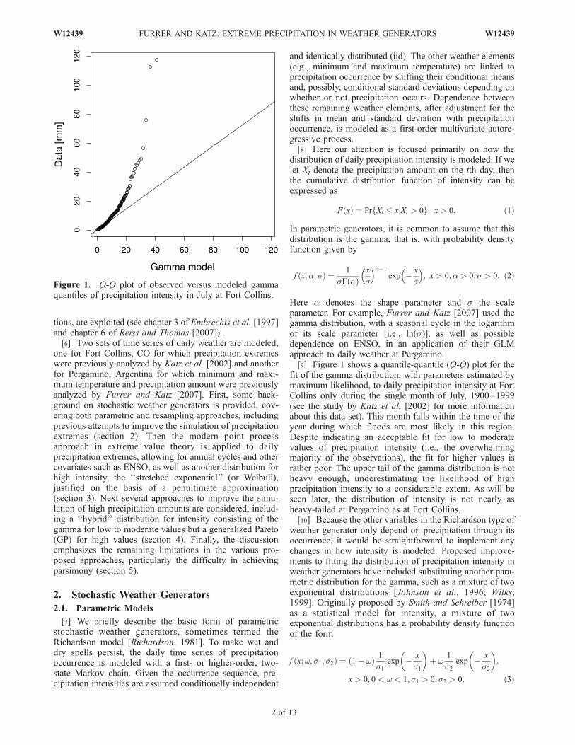
Here a denotes the shape parameter and s the scaleparameter. For example, Furrer and Katz [2007] used thegamma distribution, with a seasonal cycle in the logarithmof its scale parameter [i.e., ln(s)], as well as possibledependence on ENSO, in an application of their GLMapproach to daily weather at Pergamino.[9] Figure 1 shows a quantile-quantile (Q-Q) plot for the

fit of the gamma distribution, with parameters estimated bymaximum likelihood, to daily precipitation intensity at FortCollins only during the single month of July, 1900–1999(see the study by Katz et al. [2002] for more informationabout this data set). This month falls within the time of theyear during which floods are most likely in this region.Despite indicating an acceptable fit for low to moderatevalues of precipitation intensity (i.e., the overwhelmingmajority of the observations), the fit for higher values israther poor. The upper tail of the gamma distribution is notheavy enough, underestimating the likelihood of highprecipitation intensity to a considerable extent. As will beseen later, the distribution of intensity is not nearly asheavy-tailed at Pergamino as at Fort Collins.[10] Because the other variables in the Richardson type of

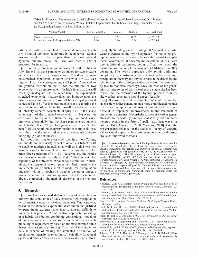
weather generator only depend on precipitation through itsoccurrence, it would be straightforward to implement anychanges in how intensity is modeled. Proposed improve-ments to fitting the distribution of precipitation intensity inweather generators have included substituting another para-metric distribution for the gamma, such as a mixture of twoexponential distributions [Johnson et al., 1996; Wilks,1999]. Originally proposed by Smith and Schreiber [1974]as a statistical model for intensity, a mixture of twoexponential distributions has a probability density functionof the form

f x;w;s1;s2ð Þ ¼ 1 wð Þ 1

s1

exp x

s1

� �þ w

1

s2

exp x

s2

� �;

x > 0; 0 < w < 1;s1 > 0; s2 > 0; ð3Þ

Figure 1. Q-Q plot of observed versus modeled gammaquantiles of precipitation intensity in July at Fort Collins.

2 of 13

W12439 FURRER AND KATZ: EXTREME PRECIPITATION IN WEATHER GENERATORS W12439

where w denotes the mixing weight and s1 and s2 the twoscale parameters. This type of mixture distribution does tendto result in a heavier tail than the gamma when fit tointensity, but still not necessarily heavy enough [Wilks,1999].[11] Alternatively, the use of a parametric form can be

relaxed and the distribution of intensity fit by nonparametrictechniques, such as kernel density smoothing. For example,Semenov [2008] used a simple binning technique. Whilethis technique does result in acceptable performance insimulating extremes consistent with observations [Semenov,2008], it has the serious limitation of not being capable ofsimulating extremes more than negligibly higher than thoseobserved. Further, it would no longer be straightforward toincorporate covariates into the weather generator (e.g.,seasonal cycles in intensity or dependence on ENSO).[12] In the stochastic modeling of precipitation, but

outside the realm of weather generators, several proposalsfor improvements in the treatment of extremes haveappeared in recent years. In a conceptual stochastic modelof rainfall, Cameron et al. [2001] used the generalizedPareto (GP), instead of the exponential, for the distributionof high intensities from a rain cell. The cumulative distri-bution function of the GP is given by

F x; x;s; uð Þ ¼ 1 1þ xx u

s

h i1=x;

x > u; 1þ xx u

s> 0;s > 0: ð4Þ

Here x denotes the shape parameter, where positive ximplies a heavy tail, negative x a bounded tail and thelimiting case of x ! 0 a light tail (i.e., the exponentialdistribution), s the scale parameter, and u the threshold forhigh intensity. Such an approach has a firm basis in extremevalue theory [e.g., Coles, 2001], which implies that theupper tail of essentially any distribution must be approxi-mately GP for sufficiently high u.[13] Making use of a heuristic physical argument, Wilson

and Toumi [2005] argued that the distribution of highprecipitation intensity ought to be approximately of thestretched exponential (or Weibull) form. Its cumulativedistribution function is given by

F x; c;s; uð Þ ¼ 1 exp x u

s

� �ch i; x > u; c > 0;s > 0; ð5Þ

where c denotes the shape parameter, s the scale parameterand u a threshold. This distribution can possess an apparentheavy tail, as formally established through a penultimateapproximation in extreme value theory (see section 3). It isappealing for stochastic weather generators because it canbe used within a GLM framework (chapter 13 ofMcCullagh and Nelder [1989]), which, for example, isnot possible for the GP distribution.[14] To avoid choosing a threshold for high intensity,

Vrac and Naveau [2007] used a dynamic mixture withgamma and GP components. Unlike an ordinary mixture,the dynamic mixture is designed to weight the gamma morefor low-intensity values, the GP more for high values. Onedrawback to this approach is that it requires the estimationof an unusually high number of parameters, at least six inpractice.

2.2. Resampling Approach

[15] The resampling approach to stochastic weather gen-eration involves drawing from the original observationswith replacement, termed the ‘‘bootstrap’’ in statistics[Efron and Tibshirani, 1993]. In practice, the resamplingscheme may be rather complicated, with the resampledobjects being vectors of weather observations (e.g., dailyminimum and maximum temperature and precipitationamount) and the resampling being restricted to nearestneighbors to preserve temporal dependence [Rajagopalanand Lall, 1999]. Several limitations, especially with respectto extremes, are inherent to any resampling scheme. Sinceonly observed values can be resampled, in particular, novalue in between the second highest value and the highestvalue is possible, etc. Moreover, a precipitation intensityhigher than the maximum observed value can never begenerated. These limitations of the resampling approachhave been previously recognized [e.g., Rajagopalan andLall, 1999]. Some sort of smoothed bootstrap would rectifythe issue of not being possible to generate values betweenthose observed. For example, Sharif and Burn [2006]introduced smoothness through perturbing the output ofthe resampling algorithm by adding a noise term. However,it is not clear how to modify the resampling approach togenerate values higher than the observed maximum, otherthan in an ad hoc fashion.

3. Upper Tail Modeling

[16] In principle we are interested in the simulation fromthe entire distribution of precipitation intensity, whichtraditionally is deficient for high intensities. Our goal beingto improve on the simulation of these high intensities, it iscrucial to first understand the upper tail behavior alone inorder be able to make plausible proposals for improvement.The statistical modeling of high precipitation intensity isnaturally linked to extreme value theory, which focuses onthe behavior and the modeling of the upper tails of distri-butions. In section 4 we will show how to use the obtainedresults for extremes in a unified modeling of the distributionof precipitation intensity.

3.1. Extreme Value Analysis

[17] We begin this section by explaining briefly how tocharacterize extreme value behavior using a two-dimensionalpoint process approach, see the work of Smith [1989],chapter 5 in the book by Leadbetter et al. [1983], andchapter 7 in the book by Coles [2001] for more details. Oneof the advantages of this representation is its unification ofthe more traditional block maxima (generalized extremevalue distribution, GEV) and peaks-over-threshold (POT,GP distribution) approaches. It uses the GEV parameteriza-tion given by the cumulative distribution function

F x; x; s*;mð Þ ¼ exp 1þ xx ms*

h i1=x� �

; 1þ xx ms*

> 0;

ð6Þ

with location parameter 1 < m <1, scale parameter s* >0 and shape parameter x having the same interpretation asfor the GP (with the limiting case of x ! 0 being theGumbel distribution). The scale parameters of the GEV and

W12439 FURRER AND KATZ: EXTREME PRECIPITATION IN WEATHER GENERATORS

3 of 13

W12439

GP parameterizations, s* and s respectively, are relatedthrough s = s* + x(u m). The point process approach isformulated in terms of the GEV parameters, which have theadvantage of not depending on a threshold, while notreducing the data to block maxima and while including thethreshold exceedance rate in the inference. As a conse-quence, non-stationarity can be easily and naturallyintroduced through covariate effects in the parameters and,theoretically, there is no difficulty in working with time-varying thresholds.[18] For the modeling of extreme values, a Poisson

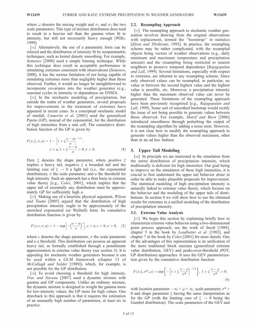
process is a natural model in a limiting sense, as seen inthe following. We start with the simplified situation of asample of iid random variables X1,. . ., Xn with commoncumulative distribution function F. Note that, in practice,the iid assumption is often not met implying the need todecluster temporally close excesses over the threshold u[Coles, 2001]. Then the distribution of the appropriatelynormalized maximum Mn = max{X1,. . ., Xn} converges tothe GEV distribution, and the distribution of the excessesover a high threshold u is approximated by a GP distributionunder mild conditions on F. The sequences used to appro-priately normalize the maximum, which ensure a non-degenerate limiting distribution, are not known in practice.Fortunately, if the appropriately normalized maximum hasasymptotic GEV distribution, so does the maximum itselfbut with different location and scale parameters. Hence, forstatistical applications of extreme value theory, it is cus-tomary to absorb the normalizing sequences into the esti-mated parameters. We use this convention in ourdescription of the point process approach. Defining asequence of two-dimensional point processes Nn by

Nn ¼ i= nþ 1ð Þ;Xið Þ : i ¼ 1; . . . ; nf g; ð7Þ

it can be seen that the number of points Nn(A) containedwithin the set A = [t1, t2] (u, 1), with [t1, t2] � (0, 1) (seeFigure 2) for sufficiently large u, is binomially distributedwith number of trials n and success probability approxi-mately given by

p � 1

nt2 t1ð Þ 1þ x

u ms*

� �h i1=x; ð8Þ

where we used the GEV/GP approximation mentionedabove. Standard convergence of a binomial distribution to aPoisson limit intuitively leads to a limiting Poisson process Nwith intensity measure np = (t2 t1)[1 + x(u mÞ=s*]1/x.We refer to mathematical details in the book by Coles[2001], for example Theorem 7.1.1, and the references

therein. Estimation of the parameters in the point processrepresentation is by maximum likelihood and requiresspecialized numerical techniques in the non-stationarycase. Coles [2001] also discusses how the simpler Poisson-GP approach, commonly used in hydrology [e.g., Madsenet al., 1997], is related to the point process representation.[19] Katz et al. [2002] applied the point process approach

to extreme value analysis of the Fort Collins daily precip-itation data over the entire year. Using a constant thresholdof u = 10 mm, they found a marked annual cycle in theextreme precipitation with a peak in July, modeled with asine wave for the location parameter m and another sinewave for the transformed scale parameter lns*. Fairlystrong evidence of a heavy tail was found, with an estimateof x of about 0.18 under the constraint of it having noannual cycle. Note that little evidence pointed to depen-dence within the excesses over u and therefore no decluster-ing was applied in this case.[20] Our goal is to apply the point process approach to the

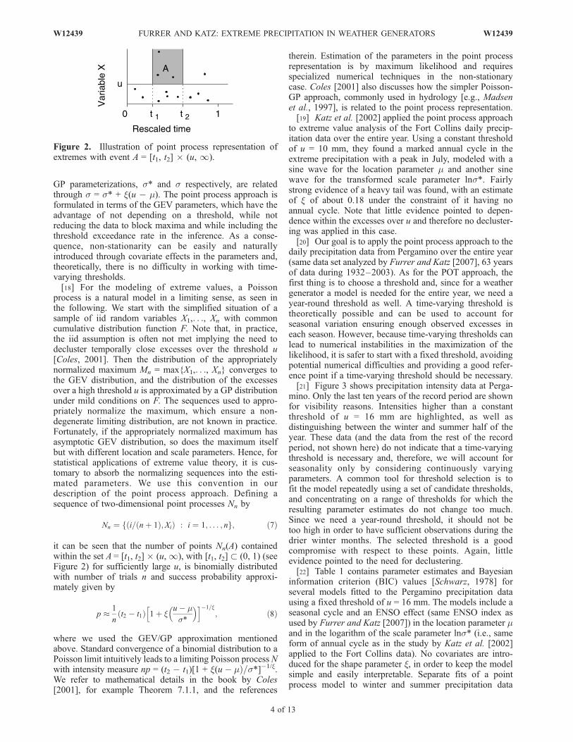
daily precipitation data from Pergamino over the entire year(same data set analyzed by Furrer and Katz [2007], 63 yearsof data during 1932–2003). As for the POT approach, thefirst thing is to choose a threshold and, since for a weathergenerator a model is needed for the entire year, we need ayear-round threshold as well. A time-varying threshold istheoretically possible and can be used to account forseasonal variation ensuring enough observed excesses ineach season. However, because time-varying thresholds canlead to numerical instabilities in the maximization of thelikelihood, it is safer to start with a fixed threshold, avoidingpotential numerical difficulties and providing a good refer-ence point if a time-varying threshold should be necessary.[21] Figure 3 shows precipitation intensity data at Perga-

mino. Only the last ten years of the record period are shownfor visibility reasons. Intensities higher than a constantthreshold of u = 16 mm are highlighted, as well asdistinguishing between the winter and summer half of theyear. These data (and the data from the rest of the recordperiod, not shown here) do not indicate that a time-varyingthreshold is necessary and, therefore, we will account forseasonality only by considering continuously varyingparameters. A common tool for threshold selection is tofit the model repeatedly using a set of candidate thresholds,and concentrating on a range of thresholds for which theresulting parameter estimates do not change too much.Since we need a year-round threshold, it should not betoo high in order to have sufficient observations during thedrier winter months. The selected threshold is a goodcompromise with respect to these points. Again, littleevidence pointed to the need for declustering.[22] Table 1 contains parameter estimates and Bayesian

information criterion (BIC) values [Schwarz, 1978] forseveral models fitted to the Pergamino precipitation datausing a fixed threshold of u = 16 mm. The models include aseasonal cycle and an ENSO effect (same ENSO index asused by Furrer and Katz [2007]) in the location parameter mand in the logarithm of the scale parameter lns* (i.e., sameform of annual cycle as in the study by Katz et al. [2002]applied to the Fort Collins data). No covariates are intro-duced for the shape parameter x, in order to keep the modelsimple and easily interpretable. Separate fits of a pointprocess model to winter and summer precipitation data

Figure 2. Illustration of point process representation ofextremes with event A = [t1, t2] (u, 1).

4 of 13


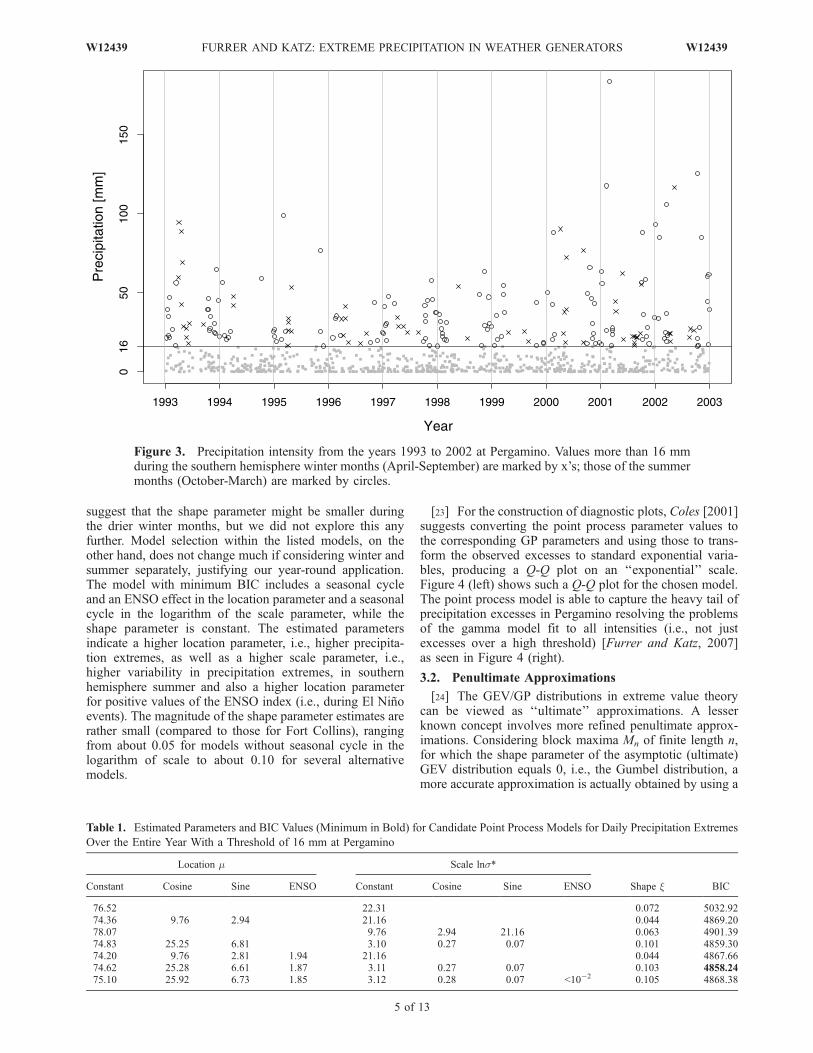
suggest that the shape parameter might be smaller duringthe drier winter months, but we did not explore this anyfurther. Model selection within the listed models, on theother hand, does not change much if considering winter andsummer separately, justifying our year-round application.The model with minimum BIC includes a seasonal cycleand an ENSO effect in the location parameter and a seasonalcycle in the logarithm of the scale parameter, while theshape parameter is constant. The estimated parametersindicate a higher location parameter, i.e., higher precipita-tion extremes, as well as a higher scale parameter, i.e.,higher variability in precipitation extremes, in southernhemisphere summer and also a higher location parameterfor positive values of the ENSO index (i.e., during El Ninoevents). The magnitude of the shape parameter estimates arerather small (compared to those for Fort Collins), rangingfrom about 0.05 for models without seasonal cycle in thelogarithm of scale to about 0.10 for several alternativemodels.

[23] For the construction of diagnostic plots, Coles [2001]suggests converting the point process parameter values tothe corresponding GP parameters and using those to trans-form the observed excesses to standard exponential varia-bles, producing a Q-Q plot on an ‘‘exponential’’ scale.Figure 4 (left) shows such a Q-Q plot for the chosen model.The point process model is able to capture the heavy tail ofprecipitation excesses in Pergamino resolving the problemsof the gamma model fit to all intensities (i.e., not justexcesses over a high threshold) [Furrer and Katz, 2007]as seen in Figure 4 (right).

3.2. Penultimate Approximations

[24] The GEV/GP distributions in extreme value theorycan be viewed as ‘‘ultimate’’ approximations. A lesserknown concept involves more refined penultimate approx-imations. Considering block maxima Mn of finite length n,for which the shape parameter of the asymptotic (ultimate)GEV distribution equals 0, i.e., the Gumbel distribution, amore accurate approximation is actually obtained by using a

Figure 3. Precipitation intensity from the years 1993 to 2002 at Pergamino. Values more than 16 mmduring the southern hemisphere winter months (April-September) are marked by x’s; those of the summermonths (October-March) are marked by circles.

Table 1. Estimated Parameters and BIC Values (Minimum in Bold) for Candidate Point Process Models for Daily Precipitation Extremes

Over the Entire Year With a Threshold of 16 mm at Pergamino

Location m Scale lns*

Shape x BICConstant Cosine Sine ENSO Constant Cosine Sine ENSO

76.52 22.31 0.072 5032.9274.36 9.76 2.94 21.16 0.044 4869.2078.07 9.76 2.94 21.16 0.063 4901.3974.83 25.25 6.81 3.10 0.27 0.07 0.101 4859.3074.20 9.76 2.81 1.94 21.16 0.044 4867.6674.62 25.28 6.61 1.87 3.11 0.27 0.07 0.103 4858.2475.10 25.92 6.73 1.85 3.12 0.28 0.07 <102 0.105 4868.38


5 of 13

W12439

non-zero shape parameter, xn say. In statistical terms thismeans that no advantage is obtained by constraining theestimation procedure to x = 0 even if it is known that thecorrect limiting distribution is the Gumbel. This approxi-mation applies equally well to the corresponding GP distri-bution for the excess over a high but finite threshold.Precise conditions and related theoretical results can befound in chapter 3 of Embrechts et al. [1997] and chapter 6of Reiss and Thomas [2007]. Examples of the use of pen-ultimate approximations in the geophysical sciences andrelated literature include that of Abaurrea and Cebrian[2002] for drought analysis and that of Cook and Harris[2004] for extreme winds in engineering design.[25] For our purposes it is sufficient to provide an

expression for xn together with a heuristic argument forhow to obtain it. In the notation of section 3.1 and assumingadditionally that the first and second derivatives of F existand that F has an infinite right endpoint, we have that thedistribution of Mn can, on the one hand, be approximated bya GEV distribution with parameters x, s*, m and, on theother hand, we have that

Pr Mn � xf g ¼ F xð Þ½ �n� expfn 1 F xð Þ½ �g ð9Þ

for n and x large such that n[1 F(x)] � constant. Equatingthese two approximations, substituting x = m, differentiatingand some further algebra yields

xn ¼F 00 mnð Þn F 0 mnð Þ½ �2

1 ¼ 1

H

� �0xð Þx¼mn

where mn ¼ F1 1 1

n

� �;H xð Þ ¼ F 0 xð Þ

1 F xð Þ ð10Þ

and H is called the hazard function. Moreover, in allpractical cases, (1/H)0(x) ! x as x ! 1. In other words, xnas given in (10) can be viewed as reflecting preasymptoticbehavior of the shape parameter.[26] The stretched exponential distribution, proposed by

Wilson and Toumi [2005] as a model for high precipitationintensity (see section 2), is not heavy-tailed in an ultimatesense, that is, the Gumbel distribution is the correct asymp-totic model. However, in a penultimate sense, this distribu-tion can have either an apparent heavy or bounded tail,depending on the value of its shape parameter c. Inparticular, the GEV shape parameter in the penultimateapproximation for block maxima of length n from astretched exponential can be expressed as

xn ¼1 c

c lnn; ð11Þ

which is easily shown by substituting the stretchedexponential cumulative distribution function (5) and itsfirst and second derivatives into (10). It is obvious fromformula (11) that c needs to be smaller than one in order forthe tail to be heavy in a penultimate sense, i.e., xn > 0. Notethat xn ! 0 as n ! 1 (i.e., consistent with the ultimateapproximation). Wilson and Toumi [2005] argued that cshould universally be 2/3, but they did not actually fix it tothat value in fitting the stretched exponential distribution tostation daily precipitation data from all over the world. Ifc = 2/3 and n = 100 (e.g., precipitation occurs on about 27%of the days within a year), then x100 � 0.11, a reasonablevalue for the shape parameter of annual maxima of dailyprecipitation. As a rough approximation for the frequencyof occurrence of precipitation within a year, we will taken = 100 days in subsequent use of (11). Because xn onlyvaries slowly with n, this approximation is not veryrestrictive.

Figure 4. (left) Q-Q plot of observed versus modeled GP quantiles of precipitation excesses over 16 mmand (right) Q-Q plot of observed versus modeled gamma quantiles of precipitation intensity for the entireyear at Pergamino.

6 of 13


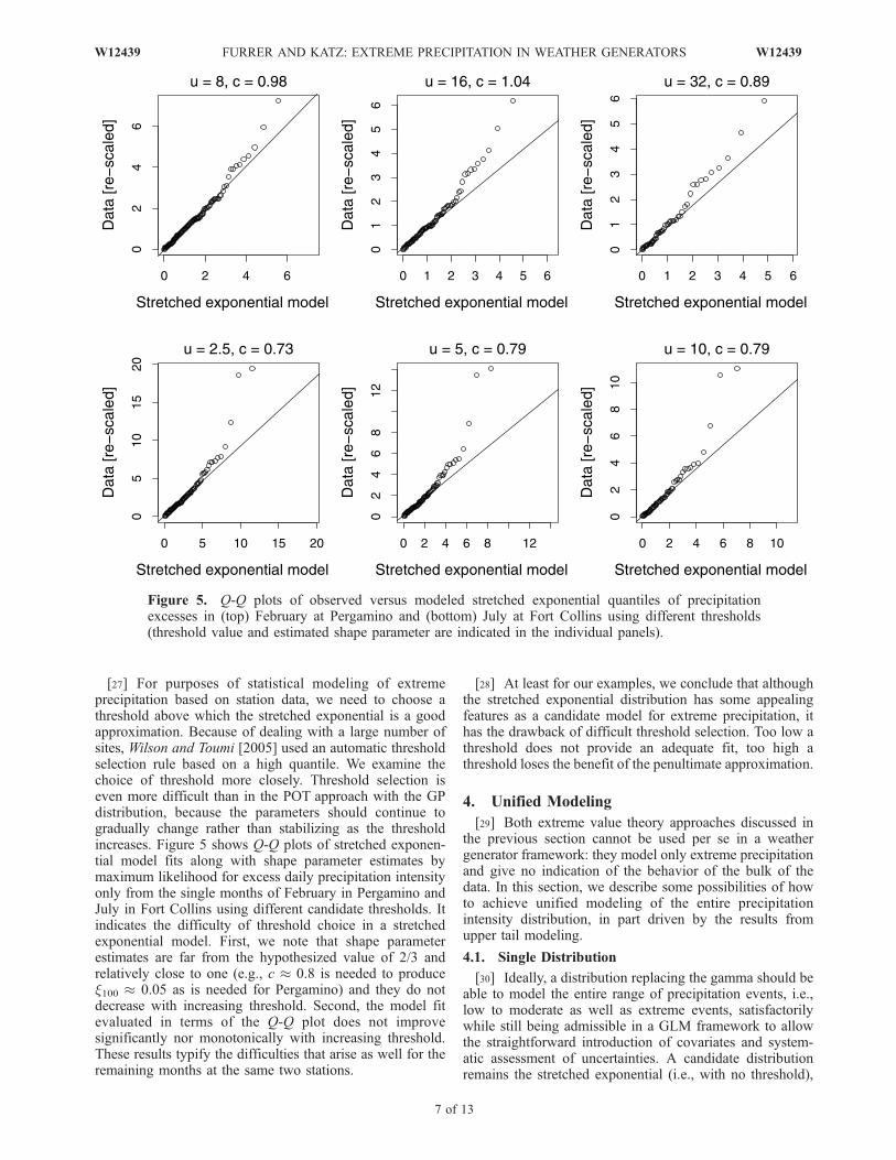
[27] For purposes of statistical modeling of extremeprecipitation based on station data, we need to choose athreshold above which the stretched exponential is a goodapproximation. Because of dealing with a large number ofsites, Wilson and Toumi [2005] used an automatic thresholdselection rule based on a high quantile. We examine thechoice of threshold more closely. Threshold selection iseven more difficult than in the POT approach with the GPdistribution, because the parameters should continue togradually change rather than stabilizing as the thresholdincreases. Figure 5 shows Q-Q plots of stretched exponen-tial model fits along with shape parameter estimates bymaximum likelihood for excess daily precipitation intensityonly from the single months of February in Pergamino andJuly in Fort Collins using different candidate thresholds. Itindicates the difficulty of threshold choice in a stretchedexponential model. First, we note that shape parameterestimates are far from the hypothesized value of 2/3 andrelatively close to one (e.g., c � 0.8 is needed to producex100 � 0.05 as is needed for Pergamino) and they do notdecrease with increasing threshold. Second, the model fitevaluated in terms of the Q-Q plot does not improvesignificantly nor monotonically with increasing threshold.These results typify the difficulties that arise as well for theremaining months at the same two stations.

[28] At least for our examples, we conclude that althoughthe stretched exponential distribution has some appealingfeatures as a candidate model for extreme precipitation, ithas the drawback of difficult threshold selection. Too low athreshold does not provide an adequate fit, too high athreshold loses the benefit of the penultimate approximation.

4. Unified Modeling

[29] Both extreme value theory approaches discussed inthe previous section cannot be used per se in a weathergenerator framework: they model only extreme precipitationand give no indication of the behavior of the bulk of thedata. In this section, we describe some possibilities of howto achieve unified modeling of the entire precipitationintensity distribution, in part driven by the results fromupper tail modeling.

4.1. Single Distribution

[30] Ideally, a distribution replacing the gamma should beable to model the entire range of precipitation events, i.e.,low to moderate as well as extreme events, satisfactorilywhile still being admissible in a GLM framework to allowthe straightforward introduction of covariates and system-atic assessment of uncertainties. A candidate distributionremains the stretched exponential (i.e., with no threshold),

Figure 5. Q-Q plots of observed versus modeled stretched exponential quantiles of precipitationexcesses in (top) February at Pergamino and (bottom) July at Fort Collins using different thresholds(threshold value and estimated shape parameter are indicated in the individual panels).


7 of 13

W12439

with extremal properties discussed in the previous section,see for example chapter 13, section 3.2 of McCullagh andNelder [1989] for its admissibility in a GLM framework andYan et al. [2006] for a climate application. In a fewinstances, the stretched exponential has been previouslyfitted to the entire distribution of precipitation intensity,particularly for accumulations over time periods shorterthan a day [Wilks, 1989; Wong, 1977]. Because the gammadistribution with shape parameter in the typical range fordaily intensity (i.e., 0.5 < a < 1) cannot produce more than anon-negligible apparent heavy tail in a penultimate sense, itis conceivable that its replacement with the stretchedexponential could still result in an improved fit for highintensity.[31] Similarly to the gamma GLM, we model the loga-

rithm of the scale of the stretched exponential distribution asa function of covariates in a GLM framework while theshape parameter is kept constant. Fitting gamma andstretched exponential GLMs to Fort Collins precipitationintensity over the entire year with seasonal cycles in thelogarithms of the respective scale parameters results in theQ-Q plots of Figure 6. In order to produce these plots, toadjust for the non-stationary form of the fitted model, theprecipitation intensity data have been re-scaled by theappropriate value of the modeled scale parameters asfunctions of the day of the year and then compared withrespective theoretical distributions of unit scale and estimated

shape parameter. As a consequence of the re-scaling, whichis different for the two models but necessary to obtain Q-Qplots in a non-stationary setting, the two plots can only becompared qualitatively. See Table 2 for estimated coeffi-cients and BIC values of gamma and stretched exponentialmodels with and without seasonal cycles. The estimate ofthe shape parameter of the stretched exponential (c = 0.77)is not too far from 2/3 but the apparent heavy tail charac-terized by the corresponding x100 � 0.06 is still rather light.From Figure 6 it is evident that the stretched exponentialmodel only results in a very slight improvement (if any)over the gamma for the fit in the upper tail of the precip-itation intensity distribution. At Pergamino, the estimatedshape parameter of the stretched exponential and thepenultimate shape parameter of the GEV take similar values(c = 0.70 and x100 � 0.09) to those at Fort Collins, again aQ-Q-plot (not shown here) reveals a slightly better fitthan that for the gamma model, but still inadequate in theupper tail.

4.2. Hybrid Approach

[32] A simple procedure to generate potentially improvedhigher precipitation intensity is to replace the values drawnfrom a gamma distribution which fall above a giventhreshold by values drawn from a GP distribution. However,this hybrid approach can create a problem of the underlyingdensity function not being continuous at the threshold u. We

Figure 6. Q-Q plots of (left) observed versus gamma and (right) stretched exponential GLM quantilesof precipitation intensity for the entire year at Fort Collins.

Table 2. Estimated Parameters and BIC Values (Minimum in Bold) for Candidate Gamma (Left) and Stretched Exponential (Right)

Models for Daily Precipitation Intensity Over the Entire Year at Fort Collins

Scale lns

Shape a BIC

Scale lns

Shape c BICConstant Cosine Sine Constant Cosine Sine

1.56 0.69 41,082.34 1.36 0.76 40,365.521.47 0.33 0.04 0.71 40,845.63 1.29 0.30 0.05 0.77 40,206.74

8 of 13


refine this simple procedure through a compromise byestimating a gamma distribution from all the data (i.e., asin a conventional weather generator), estimating a GPdistribution from the data above the threshold (i.e., as in aconventional extreme value analysis such as the pointprocess technique described in section 3), and then usingonly the estimated shape parameter x of the GP whileadjusting its scale parameter in order to achieve a contin-uous density. We call the resulting distribution a hybridgamma/GP distribution. With this approach, we need toabandon a simple GLM setting but, as elaborated below, itis still feasible to include covariates.[33] An expression for the adjustment of the scale

parameter of the GP is obtained as follows. Denote byh the hybrid gamma/GP density we want to specify, by fthe density and by F the cumulative distribution function ofthe fitted gamma distribution, and by g the density of the GPdistribution for the excesses over the threshold u with scaleparameter s and shape parameter x. Observe that g(u) = 1/sand that the mass of g is concentrated on the interval (u, 1)[see (4)]. By design the hybrid density satisfies

h xð Þ ¼ f xð Þ for x � u and

h xð Þ ¼ 1 F uð Þ½ �g xð Þ for x > u; ð12Þ

where the factor [1 F(u)] ensures that h is normalized.For h to be continuous at u it is necessary that f(u) = [1 F(u)]g(u) = [1 F(u)](1/s), i.e.,

s ¼ 1 F uð Þ½ �f uð Þ : ð13Þ

Note that s is hence the reciprocal of the hazard function[see (10)] of the gamma distribution evaluated at thethreshold u. Further note that (13) actually holds for thehybrid of any density with the GP, not just the gamma.[34] To apply (13) the gamma distribution needs to be

estimated based on the entire data set in order to obtain anestimate of the probability of intensity higher than thethreshold u. Covariate models (if any) are fitted separatelyfor the gamma and the GP distributions as in the usual GLMand extreme value analysis settings. However, since thescale parameter of the GP distribution is adjusted usingthe fitted gamma distribution, its functional dependence onthe covariates is no longer determined by the GP covariatemodel. A similar approach involving the gamma and the GPdistribution is described by Vrac and Naveau [2007], inparticular their limiting case of t = 0 (i.e., the parameter thatgoverns the speed of the transition from gamma to GP in theweight function for the dynamic mixture) models precipi-tation intensity with a gamma below a threshold and a GPabove a threshold. Drawbacks to the use of their approachin a weather generator setting are the discontinuity at thethreshold in the limiting case and the difficulty of incorpo-rating covariates.[35] Figure 7 shows the fitted gamma, GP and hybrid

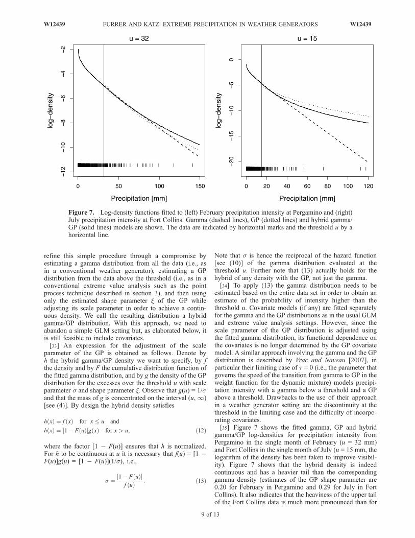
gamma/GP log-densities for precipitation intensity fromPergamino in the single month of February (u = 32 mm)and Fort Collins in the single month of July (u = 15 mm, thelogarithm of the density has been taken to improve visibil-ity). Figure 7 shows that the hybrid density is indeedcontinuous and has a heavier tail than the correspondinggamma density (estimates of the GP shape parameter are0.20 for February in Pergamino and 0.29 for July in FortCollins). It also indicates that the heaviness of the upper tailof the Fort Collins data is much more pronounced than for

Figure 7. Log-density functions fitted to (left) February precipitation intensity at Pergamino and (right)July precipitation intensity at Fort Collins. Gamma (dashed lines), GP (dotted lines) and hybrid gamma/GP (solid lines) models are shown. The data are indicated by horizontal marks and the threshold u by ahorizontal line.


9 of 13

W12439

Pergamino (at least in July and February, respectively),therefore more improvement is to be expected in applyingthis approach to the Fort Collins data. Note that the thresh-olds of 32 and 15mm, higher than when dealing with theentire year, were chosen because February and July are inthe respective wet seasons.[36] Figure 8 shows Q-Q plots of fitted gamma, hybrid

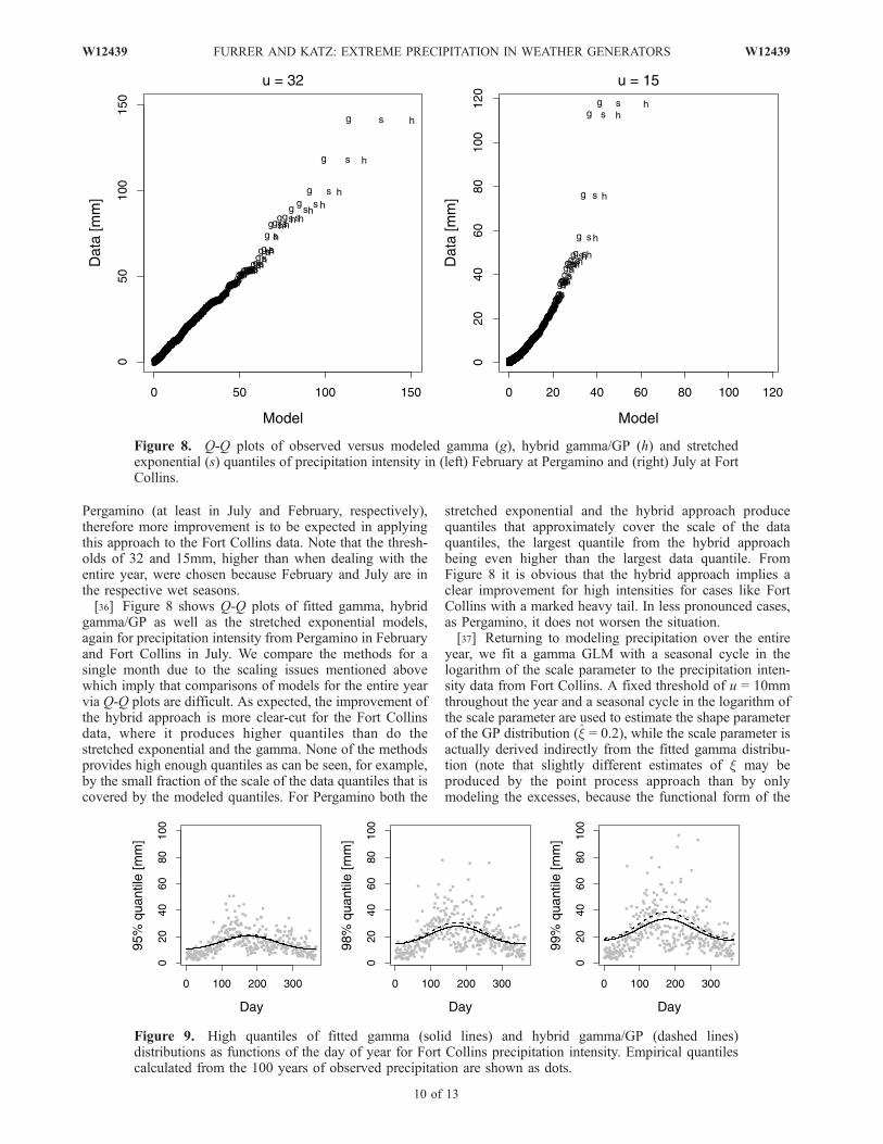
gamma/GP as well as the stretched exponential models,again for precipitation intensity from Pergamino in Februaryand Fort Collins in July. We compare the methods for asingle month due to the scaling issues mentioned abovewhich imply that comparisons of models for the entire yearvia Q-Q plots are difficult. As expected, the improvement ofthe hybrid approach is more clear-cut for the Fort Collinsdata, where it produces higher quantiles than do thestretched exponential and the gamma. None of the methodsprovides high enough quantiles as can be seen, for example,by the small fraction of the scale of the data quantiles that iscovered by the modeled quantiles. For Pergamino both the

stretched exponential and the hybrid approach producequantiles that approximately cover the scale of the dataquantiles, the largest quantile from the hybrid approachbeing even higher than the largest data quantile. FromFigure 8 it is obvious that the hybrid approach implies aclear improvement for high intensities for cases like FortCollins with a marked heavy tail. In less pronounced cases,as Pergamino, it does not worsen the situation.[37] Returning to modeling precipitation over the entire

year, we fit a gamma GLM with a seasonal cycle in thelogarithm of the scale parameter to the precipitation inten-sity data from Fort Collins. A fixed threshold of u = 10mmthroughout the year and a seasonal cycle in the logarithm ofthe scale parameter are used to estimate the shape parameterof the GP distribution (x = 0.2), while the scale parameter isactually derived indirectly from the fitted gamma distribu-tion (note that slightly different estimates of x may beproduced by the point process approach than by onlymodeling the excesses, because the functional form of the

Figure 8. Q-Q plots of observed versus modeled gamma (g), hybrid gamma/GP (h) and stretchedexponential (s) quantiles of precipitation intensity in (left) February at Pergamino and (right) July at FortCollins.

Figure 9. High quantiles of fitted gamma (solid lines) and hybrid gamma/GP (dashed lines)distributions as functions of the day of year for Fort Collins precipitation intensity. Empirical quantilescalculated from the 100 years of observed precipitation are shown as dots.

10 of 13


dependence of the extremal parameters on the covariates isnot necessarily identical). Figure 9 shows the 95%, 98% and99% quantiles of the fitted gamma and hybrid gamma/GPdistributions as functions of the day of the year, alongwith corresponding empirical quantiles calculated fromthe 100 years of observed precipitation. It indicates that thehigher the quantile the more noticeable the effect of thehybrid approach, especially during the wet summer season.[38] In order to further illustrate this ability of the hybrid

approach to model high quantiles, we simulated time seriesof daily precipitation from a GLM weather generator usingan identical (except for the lack of ENSO as a covariate)form of model for precipitation at Fort Collins as proposed byFurrer and Katz [2007] for Pergamino. 500 samples of 100years of daily data have been generated, and from thosesummer (April-September) maxima have been calculatedand GEV distributions fitted. The resulting 50-year returnlevels along with corresponding data values (includingconfidence intervals obtained by normal approximationusing an approximate variance of the estimated quantilederived by the delta method [Coles, 2001]) are shown inFigure 10. Although still not perfect, the hybrid distributionis a clear improvement over a gamma distribution for theFort Collins data. A similar exercise for the Pergamino dataleads to a less tangible improvement. However, as remarkedbefore, the heaviness of the tail for Pergamino precipitationis less pronounced and even if a hybrid approach does notnecessarily help, it does not hurt either.[39] As with the conventional POT technique, threshold

selection for the hybrid model is an important factor. Thesame techniques for threshold choice apply here, but itshould be kept in mind that the fitted gamma distribution isused to estimate the probability of exceeding the threshold

[i.e., 1 F(u)]. In other words, the mass of the heavy-tailedGP part of the hybrid distribution is determined by the fittedgamma distribution, hence estimating this probability toolow (i.e., choosing too high a threshold) implies lessemphasis on a possibly heavy tail. Therefore the thresholdu should be chosen in a region where the fit of the gammadistribution is not yet too bad, so that this probability is notunduly underestimated.

4.3. Mixture of Distributions

[40] Threshold selection for the stretched exponentialdistribution fit to daily precipitation intensity was founddifficult in practice (section 3.2). An alternative approachwould be to consider a mixture of distributions, with one ofthe components being the stretched exponential (i.e., withthreshold u = 0). In this way, threshold selection could beavoided, while still taking advantage of the capability of thestretched exponential to produce an apparent heavy uppertail. Given the common use of a mixture of two exponen-tials (3) as a model for intensity, it would be natural toreplace one of these exponentials with a stretched exponen-tial (note that the stretched exponential (5) with u = 0reduces to the exponential when the shape parameter c = 1);that is, a mixture whose cumulative distribution function isof the form

F x;w; s1; c;s2ð Þ ¼ 1 1 wð Þ exp x

s1

� � w exp x

s2

� �c �;

x > 0; 0 < w < 1;s1; c;s2 > 0: ð14Þ

It might also be plausible to constrain the shape parameter cin (14) to be equal to 2/3, the value hypothesized by Wilsonand Toumi [2005], rather than estimating it from the data.Then only three parameters (i.e., two scale parameters, s1and s2, and the mixing weight w) would need to be

Figure 10. Boxplots of 50-year return levels of summer(April-September) maximal precipitation intensity for FortCollins from 500 simulated samples using the gamma andthe hybrid gamma/GP models along with the correspondingobserved value and confidence interval (indicated byhorizontal dashed lines, range of confidence interval byvertical dashed line).

Figure 11. Q-Q plots of observed versus modeled gamma(g), mixed exponential (e) and mixed exponential/stretchedexponential with c = 2/3 (s) quantiles of precipitationintensity at Fort Collins in July.


11 of 13

W12439

estimated. Further, a stretched exponential component withc � 1 should dominate the mixture in the upper tail. Such amixture would still be simpler than the more generaldynamic mixture model that Vrac and Naveau [2007]proposed for intensity.[41] For daily precipitation intensity at Fort Collins in

July, Table 3 lists the parameter estimates for two mixturemodels, a mixture of two exponentials (3) and an exponen-tial/stretched exponential mixture (14) with c = 2/3. SeeFigure 11 for the corresponding Q-Q plots. Compared tothe gamma distribution the fit for the mixture of twoexponentials is an improvement for high intensity, but stillwoefully inadequate. On the other hand, the exponential/stretched exponential mixture does not improve upon themixed exponential in terms of overall fit (see log-likelihoodvalues in Table 3). Yet it comes much closer to capturing theapparent heavy tail, while the fit to small to moderate valuesof intensity remains acceptable (Figure 11). If the shapeparameter c of the stretched exponential in (14) were notconstrained to equal 2/3, then the log-likelihood valueimproves substantially, but the shape parameter estimate ismuch higher than 2/3 (in fact greater than one). So thebenefit of the penultimate approximation is completely lost,with the fit to the upper tail of intensity seriously deterio-rating (Q-Q plot not shown).[42] For other sites or even other months at Fort Collins,

one should not necessarily expect to obtain a satisfactory fitto small to moderate intensities as well as high intensitiesusing an exponential/stretched exponential mixture with thebrute force constraint of c = 2/3. Nevertheless, the resultsfor the single month of July at Fort Collins indicate thecapability of the stretched exponential distribution to man-ufacture an apparent heavy upper tail. Unfortunately, theimplementation of such a mixture model for precipitationintensity within a stochastic weather generator appearsproblematic, and the mixture approach therefore cannot bedirectly compared to the methods described in the previoustwo sections.

5. Discussion

[43] We have examined different ways of attempting toimprove the simulation of daily extreme high precipitationby parametric stochastic weather generators. One approach,based on the stretched exponential distribution and justifiedby penultimate extreme value theory, appears difficult toimplement in practice. An alternative approach, consistingof a hybrid distribution combining conventional modelingof precipitation intensity for low to moderate values withmodeling of high intensity based on ultimate extreme valuetheory, appears more promising. This hybrid technique notonly is capable of making the simulated distribution ofprecipitation intensity heavier, but still can allow for annualcycles and other covariates as needed in weather generators.

[44] By building on an existing GLM-based stochasticweather generator, the hybrid approach for modeling pre-cipitation intensity is reasonably straightforward to imple-ment. Nevertheless, it does require the estimation of at leastone additional parameter, being difficult to retain theparsimonious nature of the original GLM-based weathergenerator. The hybrid approach only avoids additionalcomplexity by constraining the relationship between highprecipitation intensity and any covariates to be driven by therelationship in the existing weather generator (i.e., primarilyby low to moderate intensity). Only the case of the gener-ation of time series of daily weather at a single site has beentreated, but the extension of the hybrid approach to multi-site weather generators would appear feasible.[45] Because temperature variables enter into parametric

stochastic weather generators in a more complicated mannerthan does precipitation intensity, it might well be moredifficult to implement improvements in the treatment oftemperature extremes. Nevertheless, present weather gener-ators do not necessarily simulate realistically extreme tem-perature events in the form of spells (e.g., heat waves orcold spells) [Qian et al., 2008; Semenov, 2008]. Like thepresent paper, reliance on the statistical theory of extremevalues would appear to be a promising avenue for devisingany such improved methods.

[46] Acknowledgments. We thank Philippe Naveau for advice on thisresearch. We would also like to thank three anonymous referees forvaluable suggestions that refined and improved the article. Research waspartially supported by NSF grant DMS-0355474 to the NCAR GeophysicalStatistics Project, by NSF’s Biocomplexity in the Environment programgrants BE-0410348 and CNH-0709681, and by NCAR’s Weather andClimate Assessment Science Program. The National Center for AtmosphericResearch is managed by the University Corporation for AtmosphericResearch under the sponsorship of the National Science Foundation. Allcalculations in this work have been done with the free software environmentfor statistical computing and graphics R, using the packages ismev andextRemes, see http://www.r-project.org/.

ReferencesAbaurrea, J., and A. C. Cebrian (2002), Drought analysis based on a clusterPoisson model: Distribution of the most severe drought, Clim. Res., 22,227–235.

Cameron, D., K. Bevin, and J. Tawn (2001), Modelling extreme rainfallsusing a modified pulse Bartlett-Lewis stochastic rainfall model (withuncertainty), Adv. Water Resour., 24, 203–211.

Coles, S. (2001), An Introduction to Statistical Modeling of Extreme Values,Springer, London.

Cook, N. J., and R. Harris (2004), Exact and general FT1 penultimatedistributions of extreme wind speeds drawn from tail-equivalent Weibullparents, Struct. Saf., 26, 391–420.

Efron, B., and R. J. Tibshirani (1993), An Introduction to the Bootstrap,Chapman and Hall, Boca Raton, Fla.

Embrechts, P., C. Kluppelberg, and T. Mikosch (1997), Modelling ExtremalEvents for Insurance and Finance, Springer-Verlag, Berlin.

Furrer, E. M., and R. W. Katz (2007), Generalized linear modeling approachto stochastic weather generators, Clim. Res., 34, 129–144.

Johnson, G. L., C. L. Hanson, S. P. Hardegree, and E. B. Ballard (1996),Stochastic weather simulation: Overview and analysis of two commonlyused models, J. Appl. Meteorol., 35, 1878–1896.

Table 3. Estimated Parameters and Log-Likelihood Values for a Mixture of Two Exponential Distributions

and for a Mixture of an Exponential With a Stretched Exponential Distribution (With Shape Parameter c = 2/3)

for Precipitation Intensity at Fort Collins in July

Mixture Model Mixing Weight w Scale s1 Scale s2 Log-Likelihood

Two exponentials 0.68 1.72 11.07 2053.35Exponential, stretched exponential (c = 2/3) 0.60 1.96 6.86 2062.08

12 of 13


Katz, R. W. (1996), Use of conditional stochastic models to generate climatechange scenarios, Clim. Change., 32(3), 237–255.

Katz, R. W., M. B. Parlange, and P. Naveau (2002), Statistics of extremes inhydrology, Adv. Water Resour., 25, 1287–1304.

Koutsoyiannis, D. (2004), Statistics of extremes and estimation of extremerainfall. 2: Empirical investigation of long rainfall records, Hydrol. Sci.J., 49, 591–610.

Leadbetter, M. R., G. Lindgren, and H. Rootzen (1983), Extremes andRelated Properties of Random Sequences and Processes, Springer-Verlag,New York.

Madsen, H., P. Rasmussen, and D. Rosbjerg (1997), Comparison of annualmaximum series and partial duration series methods for modeling extremehydrologic events: 1. At-site modeling,Water Resour. Res., 33, 747–757.

McCullagh, P., and J. A. Nelder (1989), Generalized Linear Models, 2nded., Chapman and Hall, London.

Qian, B., S. Gameda, and H. Hayhoe (2008), Performance of stochasticweather generators LARS-WG and AAFC-WG for reproducing dailyextremes of diverse Canadian climates, Clim. Res., 37, 17–33.

Rajagopalan, B., and U. Lall (1999), A k-nearest-neighbor simulator fordaily precipitation and other weather variables, Water Resour. Res., 35,3089–3101.

Reiss, R.-D., and M. Thomas (2007), Statistical Analysis of Extreme Valueswith Applications to Insurance, Finance, Hydrology and Other Fields,3rd ed., Birkhauser, Basel.

Richardson, C. W. (1981), Stochastic simulation of daily precipitation,temperature and solar radiation, Water Resour. Res., 17, 182–190.

Schwarz, G. (1978), Estimating the dimension of a model, Ann. Stat., 6,461–464.

Semenov, M. A. (2008), Simulation of extreme weather events by astochastic weather generator, Clim. Res., 35, 203–212.

Sharif, M., and D. H. Burn (2006), Simulating climate change scenariosusing an improved k-nearest neighbor model, J. Hydrol., 325, 179–196.

Smith, R. L. (1989), Extreme value analysis of environmental time series:An example based on ozone data (with discussion), Stat. Sci., 4, 367–393.

Smith, R. E., and H. A. Schreiber (1974), Point process of seasonal thunder-storm rainfall: 2. Rainfall depth probabilities, Water Resour. Res., 10,418–423.

Vrac, M., and P. Naveau (2007), Stochastic downscaling of precipitation:From dry events to heavy rainfalls, Water Resour. Res., 43, W07402,doi:10.1029/2006WR005308.

Wilby, R. L., T. M. L. Wigley, D. Conway, P. D. Jones, B. C. Hewitson,J. Main, and D. S. Wilks (1998), Statistical downscaling of generalcirculation model output: A comparison of methods, Water Resour.Res., 34, 2995–3008.

Wilks, D. S. (1989), Rainfall intensity, the Weibull distribution, and estima-tion of daily surface runoff, J. Appl. Meteorol., 28, 52–58.

Wilks, D. S. (1992), Adapting stochastic weather generation algorithms forclimate change studies, Clim. Change, 22, 67–84.

Wilks, D. S. (1999), Interannual variability and extreme-value characteris-tics of several stochastic daily precipitation models, Agric. For. Meteorol.,93, 153–169.

Wilks, D. S., and R. L. Wilby (1999), The weather generation game: Areview of stochastic weather models, Prog. Phys. Geogr., 23(3), 329–357.

Wilson, P. S., and R. Toumi (2005), A fundamental probability distributionfor heavy rainfall, Geophys. Res. Lett., 32, L14812, doi:10.1029/2005GL022465.

Wong, R. K. W. (1977), Weibull distribution, iterative likelihood techniqueand hydrometeorological data, J. Appl. Meteorol., 16, 1360–1364.

Yan, Z., S. Bate, R. E. Chandler, V. Isham, and H. Wheater (2006), Changesin extreme wind speeds in NW Europe simulated by generalized linearmodels, Theor. Appl. Climatol., 83, 121–137.

E. M. Furrer, Institute for Mathematics Applied to Geosciences, National

Center for Atmospheric Research, P.O. Box 3000, Boulder, CO 80307,USA. ([email protected])

R. W. Katz, Institute for Study of Society and Environment, NationalCenter for Atmospheric Research, P.O. Box 3000, Boulder, CO 80307,USA. ([email protected])


13 of 13

W12439

Documents

Click Here Full Article Improving the simulation of extreme ... to analyze and model extremal behavior of precipitation intensity (i.e., nonzero amount), which, although interesting