Embed Size (px)
Citation preview

CAEPR Working Paper #2015-013
Clearing Up the Fiscal Multiplier Morass
Eric M. Leeper
Indiana University
Nora Traum North Carolina State University
Todd B. Walker
Indiana University
July 26, 2015
This paper can be downloaded without charge from the Social Science Research Network electronic library at http://papers.ssrn.com/sol3/papers.cfm?abstract_id=2637446. The Center for Applied Economics and Policy Research resides in the Department of Economics at Indiana University Bloomington. CAEPR can be found on the Internet at: http://www.indiana.edu/~caepr. CAEPR can be reached via email at [email protected] or via phone at 812-855-4050.
©2015 by Eric M. Leeper, Nora Traum and Todd B. Walker. All rights reserved. Short sections of text, not to exceed two paragraphs, may be quoted without explicit permission provided that full credit, including © notice, is given to the source.
Clearing Up the Fiscal Multiplier Morass∗
Eric M. Leeper† Nora Traum‡ Todd B. Walker§
July 26, 2015
Abstract
We use Bayesian prior and posterior analysis of a monetary DSGE model, extended toinclude fiscal details and two distinct monetary-fiscal policy regimes, to quantify governmentspending multipliers in U.S. data. The combination of model specification, observable data,and relatively diffuse priors for some parameters lands posterior estimates in regions of theparameter space that yield fresh perspectives on the transmission mechanisms that underliegovernment spending multipliers. Posterior mean estimates of short-run output multipliers arecomparable across regimes—about 1.4 on impact—but much larger after 10 years under passivemoney/active fiscal than under active money/passive fiscal—means of 1.9 versus 0.7 in presentvalue.
Keywords : government spending; monetary-fiscal interactions; prior predictive analysis; BayesianestimationJEL Codes : C11, E62, E63
∗We would like to thank seminar participants at the Bank of Canada, the 2011 Bundesbank Spring Conference, theFederal Reserve Bank of Dallas, the 2011 Konstanz Seminar on Monetary Theory and Policy, the 2011 SED annualmeeting, and Henning Bohn, Marco Del Negro, Berthold Herrendorf, Campbell Leith, Giorgio Primiceri, MortenRavn, Harald Uhlig, Tao Zha, Marty Eichenbaum, and anonymous referees for helpful comments.
†Indiana University and NBER; [email protected].‡North Carolina State University; nora [email protected]§Indiana University; [email protected].
1 Introduction
The global recession of 2008 and the resulting fiscal stimulus packages in many countries reignited
academic interest in government spending multipliers to spawn a new and growing theoretical
and empirical literature. Despite intense professional attention, no consensus has emerged on
the dynamic impacts of government spending on macroeconomic aggregates. Because the fiscal
multiplier is a complex object that depends on nearly every detail of private and policy behavior,
different model specifications or identifying assumptions can produce wildly different quantitative
predictions of multipliers. Two broad studies neatly illustrate what we call the fiscal multiplier
morass: Coenen et al. (2012) examine seven dynamic stochastic general equilibrium (DSGE) models
to report “a robust finding across all models that fiscal policy can have sizable output multipliers;”
Cogan et al. (2010) study closely related models and similar data to conclude, “multipliers are less
than one. . . . The impact in the first year is very small. And as the government purchases decline
in the later years of the simulation, the multipliers turn negative.”1 Starkly different conclusions
from similar models and data constitute a morass.
This paper uses Bayesian prior and posterior analysis to clear up the morass by tracing differ-
ences in estimates of multipliers to different model specifications. We augment a monetary DSGE
model from the class that Smets and Wouters (2005, 2007) and Christiano et al. (2005) develop with
a rich set of fiscal details: government spending that may be valued as a public good, explicit rules
for fiscal instruments, a maturity structure of government debt, and distorting steady-state taxes.
We also go beyond existing empirical analyses of multipliers to consider alternative monetary-fiscal
regimes: either active monetary policy coupled with passive fiscal policy (regime M) or active fiscal
policy together with passive monetary policy (regime F).2
Prior predictive analysis reports the probability distribution of multiplier values that a particular
specification can produce before confronting data. That analysis finds, for example, that it is
impossible for standard real business cycle models to produce large multipliers, while new Keynesian
models with a substantial fraction of rule-of-thumb agents are quite unlikely to generate small
multipliers, regardless of the information that data contain about multipliers.
Prior predictive analysis guides our choice of model to take to the data. We seek a specification
that a priori is consistent with either small or large multipliers, depending on estimated parameter
values. The prior analysis suggests that a model that permits government spending to complement
or substitute for private consumption and conditions on either regime M or regime F supports the
widest ranges for multipliers.
We maintain the agnostic spirit of the prior predictive analysis when we estimate by employing
relatively diffuse prior distributions over some model parameters and by considering distinct priors
1Coenen et al. (2012) delves into some of the subtleties responsible for the differences in multipliers across studies.Gechert and Will (2012, p. 28) examine 89 multiplier studies spanning many methodologies to conclude that “reportedmultipliers very much depend on the setting and method chosen.”
2An active authority is defined as an authority who is not constrained by current budgetary conditions and freelychooses the decision rule it wants. A passive authority is constrained by the consumers’ and firms’ optimizations andby the actions of the active authority, so the passive authority must stabilize debt. See Leeper (1991), Sims (1994),Woodford (1995), and Cochrane (1999) for more discussion.
Leeper, Traum & Walker: Fiscal Multiplier Morass
that place the economy in one of the two monetary-fiscal regimes. The fiscal details in our model and
the data set, both of which rarely appear in estimated DSGE models, permit the posterior to land
in regions of the parameter space that produce 90-percent fresh perspectives on the transmission
mechanisms that underlie government spending multipliers. Despite our diffuse a priori views
about the sizes and the dynamics of multipliers, U.S. data are highly informative: they narrow the
posterior range of multipliers substantially to help us clear up the multiplier morass.
Over the full sample period, 1955q1–2014q2, the posterior estimates deliver high degrees of
nominal rigidities, strong habit formation and complementarity between government and private
consumption in both policy regimes. These estimates produce comparable short-run output multi-
pliers across regimes—mean impact multipliers are about 1.4—but substantially larger multipliers
in regime F than in regime M at long horizons—after 10 years the mean present-value multiplier
is 1.9 in F, but 0.7 in M. Consumption effects are positive in both regimes, with multipliers that
hover around 0.2 to 0.3 in present value. Investment multipliers are decidedly negative in regime
M but more likely to be positive in regime F: 90-percent credible sets at 10 years are [−1.4,−0.8]
in M and [−0.2, 0.3] in F.
Although private parameter estimates are quite similar across policy regimes, the two monetary-
fiscal mixes imply different fiscal financing schemes that transmit government spending through
the economy in different ways. Posterior estimates for the full sample yield somewhat unusual
passive fiscal behavior in regime M: higher government debt raises future lump-sum transfers
and the full brunt of debt stabilization is borne by government spending reversals of the kind that
Corsetti et al. (2012) emphasize. In regime F stabilization occurs from revaluations of debt through
surprise changes in inflation and bond prices. Steady-state distorting tax rates ensure that revenues
endogenously respond to economic conditions in both regime, even though the constant tax rates
cannot stabilize debt.
At the risk of some oversimplification, we can succinctly describe the transmission mechanisms.
Three aspects of behavior lie behind government spending impacts in regime M: strong rigidities—
price and wage stickiness and habit formation—complementarity of government spending to private
consumption, and fiscal financing through spending reversals. Complementarity ensures that higher
spending initially raises consumption even though long-run real interest rates also rise. Anticipated
cuts in future government spending, coupled with higher transfers, raise household wealth and
temper long-run real rate increases to support consumers’ strong desire to smooth consumption at
a level above steady state for many years after the initial spending impulse. Because the output
boost is short-lived, higher consumption in the long run comes out of reduced investment.
This estimated transmission mechanism differs from convention—as in, for example, Galı et al.
(2007), Woodford (2011) or Corsetti et al. (2012)—along several dimensions. First, most studies
do not permit government spending to interact directly with consumption through preferences.
Second, high estimated nominal rigidities dampen inflationary and real-interest rate effects. Third,
estimated fiscal financing produces positive, rather than the usual negative, wealth effects. These
differences account for the persistently positive consumption multipliers.
2
Leeper, Traum & Walker: Fiscal Multiplier Morass
Based on previous work on government spending multipliers when monetary policy is passive, it
may be surprising that our reported multipliers are not several times larger in regime F than in M.3
Although very large fiscal effects are possible when our model resides in regime F, the moderate
impacts that the posterior estimates produce stem primarily from three factors: high nominal
rigidities, the existence of a maturity structure for nominal government debt, and the presence of
steady-state taxes on labor and capital income.
Higher government spending financed by nominal bond sales raises household wealth when
fiscal policy is active and future surpluses are not expected to adjust to stabilize debt. Rigid prices
convert higher nominal debt into sustained increases in real debt and in household wealth. Higher
wealth boosts consumption demand, which price stickiness translates into higher labor demand,
rather than higher goods prices. Because the real value of debt cannot fall significantly through a
higher price level, it declines instead through lower bond prices; the maturity structure for bonds
permits revaluation to occur through higher future inflation. With inflation rising only modestly,
long-run real interest rates rise even under passive monetary policy, just as they do in regime M
when monetary policy is active.
Long-run output multipliers are substantially larger in regime F because real wages and employ-
ment increase strongly and persistently to increase human wealth and sustain consumption demand.
Consumption multipliers remain positive many years after the government spending increase has
dissipated without crowding out investment, as occurs in regime M. Multipliers are not implausi-
bly large in regime F, as previous research may suggest, because steady-state taxes levied against
factor incomes raise aggregate tax revenues along with the expansion in real economic activity to
temper the wealth effects that active fiscal policy engenders. Steady-state tax rates capture the
reality that even if a government does not systematically adjust tax schedules when government
debt rises, revenues nonetheless rise with incomes because existing tax rates remain in place.
As in regime M, the posterior estimates in regime F deliver a very different transmission mech-
anism for government spending than appears elsewhere in the literature. Sizeable multipliers for
output and consumption arise despite higher long-run real interest rates. Dupor and Li (2015)
argue that passive monetary policy gives government spending expansions unreasonably large in-
flationary consequences that are inconsistent with empirical evidence. This does not occur in our
estimates because the model includes fiscal details that most analyses neglect.
The paper’s emphasis on monetary-fiscal interactions is tightly connected to data. Previous
work relies on theoretical or calibrated results to argue that government spending’s impacts can
be quite different across regimes M and F. This paper confronts those theoretical possibilities with
data to find that model fit can be comparable across regions of the parameter space that produce
different government spending transmission mechanisms and multiplier dynamics.
3Work on government spending increases by Kim (2003), Christiano et al. (2011), Davig and Leeper (2011) andDupor and Li (2015) finds that in regime F or at the zero lower bound for nominal interest rates, output multiplierscan exceed 2, real interest rates fall and inflation rises substantially.
3
Leeper, Traum & Walker: Fiscal Multiplier Morass
2 The Models
The models we use for prior predictive analysis share several details with the class of models used
to evaluate the size of fiscal multipliers: (1) forward-looking, optimizing agents; (2) households who
receive utility from consumption and leisure and additionally may value government consumption;
(3) a distinction between households who can save (“savers”) and who are constrained to consume
their income each period (“non-savers”); (4) production sectors that use capital and labor inputs;
(5) monopolistic competition in the goods and labor sectors; (6) empirically relevant nominal and
real frictions; (7) fiscal and monetary authorities who set their instruments using simple feedback
rules; and (8) the economy at its cashless limit.
Our model structure nests many of the frameworks that researchers have used to quantify fiscal
multipliers, but expands on those frameworks by filling in many details of the fiscal side of the
model. Those details include allowing for public goods that may be valued in utility, explicit rules
for several fiscal instruments, a maturity structure for nominal government debt, and steady-state
distorting taxes.
2.1 Firms and Price Setting
The production sector consists of intermediate and final goods producing firms. A perfectly com-
petitive final goods producer uses a continuum of intermediate goods Yt(i), where i ∈ [0, 1], to
produce the final goods Yt, with the constant-return-to-scale technology (∫ 10 Yt(i)
1
1+ηpt di)1+η
pt ≥ Yt,
where ηpt denotes an exogenous, time-varying markup to the prices of intermediate goods.
The price of intermediate good i is Pt(i) and the price of final goods Yt is Pt. The final goods
producing firm chooses Yt and Yt(i) to maximize profits subject to the constant-return-to-scale
technology. Dixit-Stiglitz aggregation yields the demand Yt(i) = Yt(
Pt(i)/Pt)−(1+ηpt )/η
pt .
Intermediate goods producers are monopolistic competitors in their product market. Firm i has
access to the technology Yt(i) = Kt(i)α(AtLt(i))
1−α − AtΩ, where α ∈ [0, 1] and Ω > 0 represents
fixed costs to production that grow at the rate of technological progress. At is a permanent shock
to technology. The logarithm of its growth rate, uat = lnAt− lnAt−1, follows the stationary AR(1)
process uat = (1− ρa)γ + ρauat−1 + ǫat , ǫat ∼ N(0, σ2a), where γ defines the logarithm of the steady-
state gross growth rate of technology. Firms face perfectly competitive factor markets for capital
and labor. Cost minimization implies that the firms have identical nominal marginal costs per unit
of output, MCt = (1− α)α−1α−α(Rkt )αW 1−α
t A−1+αt .
Prices evolve by a Calvo (1983) mechanism. An intermediate firm faces probability (1−ωp) each
period that it may reoptimize its price. Firms that cannot reoptimize partially index their prices
to past inflation according to the rule Pt(i) = (πt−1)χp (π)1−χpPt−1(i), where πt−1 ≡ Pt−1/Pt−2 is
the inflation rate, π is the steady state inflation rate, and χp ∈ [0, 1].
Firms that reoptimize their price in period t maximize expected discounted nominal profits
subject to the demand for Yt(i). Given the production function, average and marginal costs coincide,
4
Leeper, Traum & Walker: Fiscal Multiplier Morass
which allows expected discounted nominal profits to be written as
Et
∞∑
s=0
(βωp)sλt+sλt
[(
s∏
k=1
πχpt+k−1π
1−χp
)
Pt(i)Yt+s(i)−MCt+sYt+s(i)
]
(1)
where λ is the marginal utility of wealth of saver households, defined below.
2.1.1 Labor Agency Each household supplies a continuum of differentiated labor services
indexed by l. These differentiated labor services are supplied by both savers and non-savers,
and demand is uniformly allocated among households. A competitive labor agency combines the
differentiated labor services into a homogenous labor input that is sold to intermediate firms,
according to the technology Lt = (∫ 10 Lt (l)
11+ηwt dl)1+η
wt where ηwt denotes a time-varying exogenous
markup to wages. The competitive labor agency’s demand function comes from solving its profit
maximization problem, which yields Lt (l) = Ldt (Wt(l)/Wt)−(1+ηwt )/ηwt where Ldt is the demand for
composite labor services, which is given by intermediate firms, and Wt is the aggregate nominal
wage that satisfies Wt = (∫ 10 Wt(l)
1ηwt dl)η
wt .
2.2 Households
The economy is populated by a continuum of households on the interval [0, 1], of which a fraction
µ are non-savers and a fraction 1−µ are savers. Superscript S indicates a variable associated with
savers and N with non-savers.
2.2.1 Savers An optimizing saver household j derives utility from composite consumption,
C∗S(j), consisting of private CSt (j) and public Gt consumption goods, C∗S(j) ≡ CSt (j)+αGGt. Pa-
rameter αG governs the degree of substitutability of the consumption goods: when αG < 0, private
and public consumption are complements; when αG > 0, the goods are substitutes. The household
values consumption relative to a habit stock defined in terms of lagged aggregate consumption of
savers (θC∗St−1 where θ ∈ [0, 1)). Each household j supplies a continuum of differentiated labor
inputs, LSt (j, l), l ∈ [0, 1]. The aggregate quantity of these labor services is LSt (j) ≡∫ 10 L
St (j, l)dl.
Households maximize lifetime utility Et∑∞
t=0 βtubt(ln (C
∗St (j)− θC∗S
t−1)−(LSt (j)1+ξ)/(1+ξ)), where
β is the discount rate, ξ is the inverse of the Frisch labor elasticity and ubt is an exogenous shock
to preferences.
Savers have access to one-period nominal private bonds, Bs,t, that pay 1 unit of currency in t+1,
sell at price R−1t in t, and are in zero net supply. They also have access to a portfolio of long-term
nominal government bonds, Bt, which sells at price PBt in t. Maturity of these zero-coupon bonds
decays at the constant rate ρ ∈ [0, 1] to yield the duration (1− βρ)−1.
Savers receive after-tax wage and rental income, lump-sum transfers from the government ZS ,
and profits from firms D. Savers spend income on consumption, investment in future capital IS ,
5
Leeper, Traum & Walker: Fiscal Multiplier Morass
and government bonds. The nominal flow budget constraint for saver j is
Pt(1 + τCt )CSt (j) + PtI
St (j) + PB
t Bt(j) +R−1
t Bs,t(j) = (1 + ρPBt )Bt−1(j) +Bs,t−1(j)
+ (1 − τLt )
∫
1
0
Wt(l)LSt (j, l)dl + (1− τKt )Rk
t vt(j)KSt−1
(j)− ψ(vt)KSt−1
+ PtZSt (j) +Dt(j)
Nominal consumption, PCC, is subject to a sales tax τC . Wt(l) is the nominal wage rate for labor
input l, and∫ 10 Wt(l)L
St (j, l)dl is the total nominal labor income for household j, which is taxed at
the rate τL. Since each saver-type household supplies all differentiated labor inputs in the economy,
all saver households have the same total after-tax labor income in equilibrium.
Effective capital is related to the physical capital stock K by Kst (j) = vt(j)K
St−1(j), where vt(j)
is the utilization rate of capital. Utilization incurs a cost of Ψ(vt) per unit of physical capital. In
steady state, v = 1 and Ψ(1) = 0. We define the parameter ψ ∈ [0, 1) such that Ψ′′(1)
Ψ′(1)
≡ ψ1−ψ , as in
Smets and Wouters (2003). As ψ → 1, utilization costs become infinite, and the capital utilization
rate becomes constant. Rental income on effective capital is taxed at the rate τK . Capital obeys
the law of motion
KSt (j) = (1− δ)KS
t−1(j) + uit
[
1− s
(
ISt (j)
ISt−1(j)
)]
ISt (j)
where s (·) ISt is an investment adjustment cost, as in Smets and Wouters (2003) and Christiano
et al. (2005) and satisfies s′ (eγ) = 0, and s′′ (eγ) ≡ s > 0. Investment costs decrease as s declines
and are subject to an investment-specific efficiency shock uit.
Saver households reset their nominal wages for each differentiated labor service with probability
(1 − ωw) each period. Wages that cannot be reoptimized are partially indexed to past inflation
according to the rule Wt (l) = Wt−1 (l) (πt−1euat−1)χ
w(πeγ)1−χw , where χw ∈ [0, 1] measures the
degree of indexation. When wages are reset, households choose the nominal wage rate Wt (l) to
maximize their utility.
2.2.2 Non-savers Non-savers have the same preferences as savers. Non-savers are rule-of-
thumb agents who consume their entire disposable income each period, which consists of after-tax
labor income and lump-sum transfers from the government ZN . Like savers, non-savers supply all
differentiated labor services. The budget constraint for a non-saver j ∈ (µ, 1] is
(1 + τCt )PtCNt (j) = (1− τ lt)
∫ 1
0Wt(l)L
Nt (j, l)dl + PtZ
Nt (j) (2)
Substantial variation in modeling wage-setting decisions exists in the literature. We assume that
savers optimally set wage rates, while non-savers follow a rule-of-thumb to set their wage rates to
be the average wage rates chosen by savers, as in Erceg et al. (2006) and Forni et al. (2009). Since
non-savers face the same labor demand schedule as savers, they work the same number of hours as
the average for savers.
6
Leeper, Traum & Walker: Fiscal Multiplier Morass
Non-savers’ nominal consumption PCCN is taxed at the same rate as savers, τC , and their
nominal wage income is taxed at the same rate as savers, τL. Because non-savers elastically meet
the demand for their labor and set their nominal wages according to savers’ optimization, budget
constraint (2) determines non-savers’ consumption.
2.3 Monetary & Fiscal Policy
The monetary authority follows a Taylor-type rule, in which the nominal interest rate Rt responds to
its lagged value, the current inflation rate, and current output. We denote a variable in percentage
deviations from steady state by a hat. The interest rate obeys Rt = ρrRt−1+(1−ρr)[
φππt + φyYt
]
+
umt , where um is a monetary policy shock, defined by the process umt = ρemu
mt−1 + ǫmt , ǫmt ∼
N(0, σ2m) .
The government collects tax revenues from capital, labor, and consumption taxes, and sells the
nominal bond portfolio, Bt, to finance its interest payments and expenditures, Gt, ZSt , Z
Nt . Fiscal
choices satisfy the identity PBt Bt + τKt RKt Kt + τLt WtLt+Ptτ
Ct Ct = (1+ ρPBt )Bt−1 +PtGt +PtZt,
where lump-sum transfers are assumed to be identical across households, so that Zt =∫ 10 Zt(j)dj =
ZSt = ZNt .
Fiscal rules are simple. They include a response of fiscal instruments to the market value of the
debt-to-GDP ratio—to ensure that policies stabilize debt—and an autoregressive term to allow for
serial correlation. Fiscal instruments follow the rules
Gt = ρGGt−1−(1−ρG)γGsbt−1
+uGt , Zt = ρZ Zt−1−(1−ρZ)γZ sbt−1
+uZt , τJt = ρJ τJt−1
+(1−ρJ )γJ sbt−1
,
where J = K,L, sbt−1 ≡PBt−1Bt−1
Pt−1Yt−1, ust = ρesu
st−1+ǫ
st and ǫ
st ∼N(0, σ2s ) for s = G, Z. Consumption
taxes are restricted to a constant, steady state value.4
2.4 Aggregation
Aggregate consumption is Ct =∫ 10 Ct(j)dj = (1 − µ)CSt + µCNt . Because only savers have access
to the asset and capital markets, aggregate bonds, private capital, investment, and dividends are
Υt =∫ 1−µ0 Υt(j)dj for Υ = B,K, I,D. The goods market clearing condition is Yt = Ct+ It+Gt+
ψ(vt)Kt−1.
2.5 Nested Models
Our broad model nests models that are commonly used to examine the size of the fiscal multiplier.
Table 1 lists the specific parameter restrictions that deliver each of the five nested models. Model
1 eliminates all nominal frictions (ωw = ωp = ηw = ηp = χw = χp = 0) and monetary policy
(φπ = φy = ρr = 0) to reduce to a standard RBC model. Model 2 is a standard new Keynesian
4We do not allow consumption taxes to respond to debt. In U.S. federal government data, consumption taxesconsist of excise taxes and custom duties, which average one percent of GDP. The online appendix documents thatconsumption tax financing has little quantitative effect on multipliers.
7
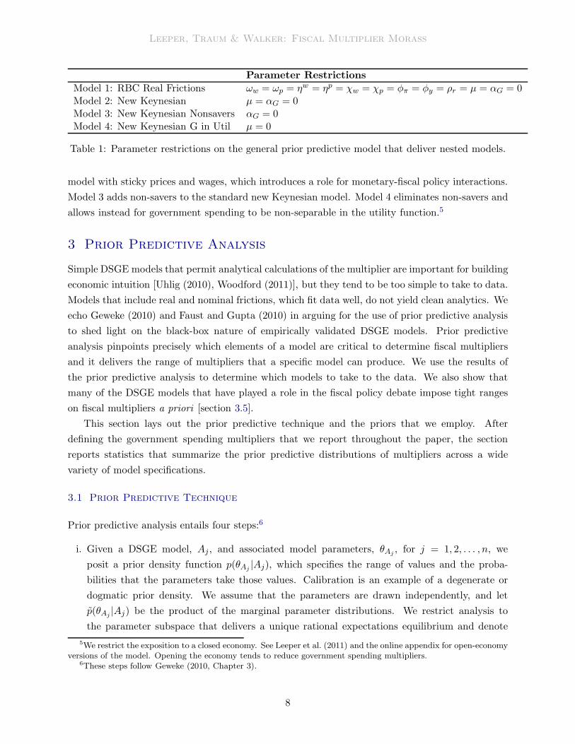
Leeper, Traum & Walker: Fiscal Multiplier Morass
Parameter Restrictions
Model 1: RBC Real Frictions ωw = ωp = ηw = ηp = χw = χp = φπ = φy = ρr = µ = αG = 0Model 2: New Keynesian µ = αG = 0Model 3: New Keynesian Nonsavers αG = 0Model 4: New Keynesian G in Util µ = 0
Table 1: Parameter restrictions on the general prior predictive model that deliver nested models.
model with sticky prices and wages, which introduces a role for monetary-fiscal policy interactions.
Model 3 adds non-savers to the standard new Keynesian model. Model 4 eliminates non-savers and
allows instead for government spending to be non-separable in the utility function.5
3 Prior Predictive Analysis
Simple DSGE models that permit analytical calculations of the multiplier are important for building
economic intuition [Uhlig (2010), Woodford (2011)], but they tend to be too simple to take to data.
Models that include real and nominal frictions, which fit data well, do not yield clean analytics. We
echo Geweke (2010) and Faust and Gupta (2010) in arguing for the use of prior predictive analysis
to shed light on the black-box nature of empirically validated DSGE models. Prior predictive
analysis pinpoints precisely which elements of a model are critical to determine fiscal multipliers
and it delivers the range of multipliers that a specific model can produce. We use the results of
the prior predictive analysis to determine which models to take to the data. We also show that
many of the DSGE models that have played a role in the fiscal policy debate impose tight ranges
on fiscal multipliers a priori [section 3.5].
This section lays out the prior predictive technique and the priors that we employ. After
defining the government spending multipliers that we report throughout the paper, the section
reports statistics that summarize the prior predictive distributions of multipliers across a wide
variety of model specifications.
3.1 Prior Predictive Technique
Prior predictive analysis entails four steps:6
i. Given a DSGE model, Aj , and associated model parameters, θAj , for j = 1, 2, . . . , n, we
posit a prior density function p(θAj |Aj), which specifies the range of values and the proba-
bilities that the parameters take those values. Calibration is an example of a degenerate or
dogmatic prior density. We assume that the parameters are drawn independently, and let
p(θAj |Aj) be the product of the marginal parameter distributions. We restrict analysis to
the parameter subspace that delivers a unique rational expectations equilibrium and denote
5We restrict the exposition to a closed economy. See Leeper et al. (2011) and the online appendix for open-economyversions of the model. Opening the economy tends to reduce government spending multipliers.
6These steps follow Geweke (2010, Chapter 3).
8
Leeper, Traum & Walker: Fiscal Multiplier Morass
this subspace as ΘDj . Let IθAj ∈ ΘDj be an indicator function that is one if θAj is in
the determinacy region and zero otherwise. Then, the joint prior distribution is defined as
p(θAj |Aj) =1c p(θAj |Aj)IθAj ∈ ΘDj, where c =
∫
θAj∈ΘDjp(θAj |Aj)dθAj
ii. The log-linearized DSGE model that section 2 describes and the nested models in table 1
constitute the set of models under consideration. Those models generate ex-ante predictive
distributions for the models’ observables, yT , from p(yT |Aj) =∫
ΘAjp(θAj |Aj)p(yT |θAjAj)dθAj
iii. We specify a vector of interest, ω, with corresponding distribution p(ωT |yT , θAj , Aj). Our vector
of interest consists of various measures of the fiscal multiplier, which we define in section 3.4.
As the conditional distribution makes explicit, the fiscal multiplier depends on the choice of
model (Aj), model-implied observables (yT ), and parameters (θAj).
iv. To generate prior predictive distributions for fiscal multipliers, the algorithm draws from θ(m)Aj
∼
p(θAj |Aj), and y(m)T ∼ p(yT |θ
(m)Aj
, Aj). Drawing sequentially from these distributions delivers
p(yT |Aj) and any function of yT including the vector of interest, ω(m). A model specification
and a prior distribution produce prior distributions for fiscal multipliers.
The distribution p(yT |Aj) gives the prior distribution of observables, which implies the distri-
bution of fiscal multipliers, p(ωT |yT , θAj , Aj). Computationally, it is straightforward and nearly
costless to simulate from p(yT |Aj). Given a prior density over model parameters, prior predictive
analysis produces the entire range of a model’s possible multipliers, to shed light on a model’s
predictions before confronting data. This narrows the set of models to estimate. For example, if
prior predictive analysis suggests that it is nearly impossible for a model to produce large multi-
pliers, then conclusions drawn from estimates of that model need to be tempered by the fact that
regardless of the information in actual data, the model will imply that multipliers are small. Prior
predictive analysis helps to gauge whether such a model is appropriate to study the magnitude of
fiscal multipliers.
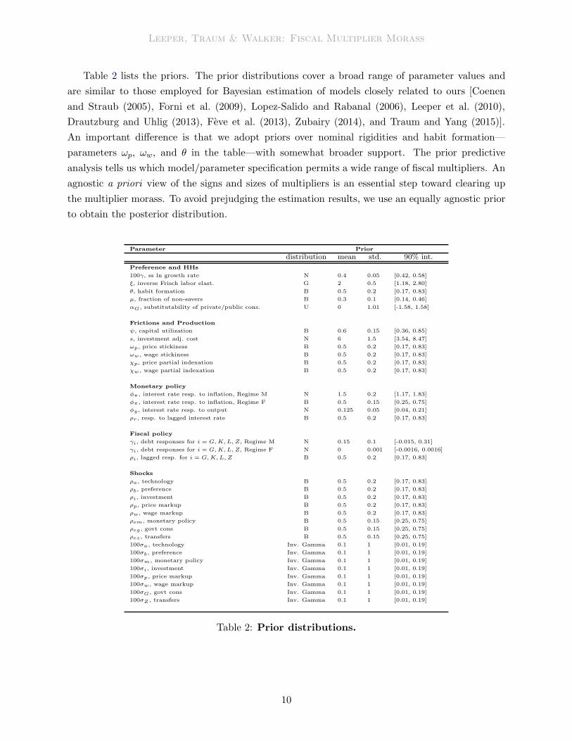
3.2 Prior Distributions
In all model specifications we fix a few parameters. The discount factor, β, is set to 0.99. The
capital income share of total output, α, is set to 0.33. The quarterly depreciation rate for private
capital, δ, is set to 0.025 so that the annual depreciation rate is 10 percent. Steady state inflation,
π, is 1. Because the price and wage markups cannot be separately identified in the estimation, we
calibrate them as ηw = ηp = 0.14.
Steady-state fiscal variables are calibrated to the mean values from U.S. data over the period
1955q1–2014q2. Federal government consumption as a share of model output (that is, GDP ex-
cluding net exports) is 0.11, the federal debt to annualized model output share is 1.47, the average
federal labor tax rate is 0.186, the capital tax rate is 0.218, and the consumption tax rate is 0.023.
See the online appendix for details of the data construction.
9
Leeper, Traum & Walker: Fiscal Multiplier Morass
Table 2 lists the priors. The prior distributions cover a broad range of parameter values and
are similar to those employed for Bayesian estimation of models closely related to ours [Coenen
and Straub (2005), Forni et al. (2009), Lopez-Salido and Rabanal (2006), Leeper et al. (2010),
Drautzburg and Uhlig (2013), Feve et al. (2013), Zubairy (2014), and Traum and Yang (2015)].
An important difference is that we adopt priors over nominal rigidities and habit formation—
parameters ωp, ωw, and θ in the table—with somewhat broader support. The prior predictive
analysis tells us which model/parameter specification permits a wide range of fiscal multipliers. An
agnostic a priori view of the signs and sizes of multipliers is an essential step toward clearing up
the multiplier morass. To avoid prejudging the estimation results, we use an equally agnostic prior
to obtain the posterior distribution.
Parameter Prior
distribution mean std. 90% int.
Preference and HHs
100γ, ss ln growth rate N 0.4 0.05 [0.42, 0.58]
ξ, inverse Frisch labor elast. G 2 0.5 [1.18, 2.80]
θ, habit formation B 0.5 0.2 [0.17, 0.83]
µ, fraction of non-savers B 0.3 0.1 [0.14, 0.46]
αG, substitutability of private/public cons. U 0 1.01 [-1.58, 1.58]
Frictions and Production
ψ, capital utilization B 0.6 0.15 [0.36, 0.85]
s, investment adj. cost N 6 1.5 [3.54, 8.47]
ωp, price stickiness B 0.5 0.2 [0.17, 0.83]
ωw, wage stickiness B 0.5 0.2 [0.17, 0.83]
χp, price partial indexation B 0.5 0.2 [0.17, 0.83]
χw , wage partial indexation B 0.5 0.2 [0.17, 0.83]
Monetary policy
φπ , interest rate resp. to inflation, Regime M N 1.5 0.2 [1.17, 1.83]
φπ , interest rate resp. to inflation, Regime F B 0.5 0.15 [0.25, 0.75]
φy , interest rate resp. to output N 0.125 0.05 [0.04, 0.21]
ρr, resp. to lagged interest rate B 0.5 0.2 [0.17, 0.83]
Fiscal policy
γi, debt responses for i = G,K, L, Z, Regime M N 0.15 0.1 [-0.015, 0.31]
γi, debt responses for i = G,K, L, Z, Regime F N 0 0.001 [-0.0016, 0.0016]
ρi, lagged resp. for i = G,K, L, Z B 0.5 0.2 [0.17, 0.83]
Shocks
ρa, technology B 0.5 0.2 [0.17, 0.83]
ρb, preference B 0.5 0.2 [0.17, 0.83]
ρi, investment B 0.5 0.2 [0.17, 0.83]
ρp, price markup B 0.5 0.2 [0.17, 0.83]
ρw, wage markup B 0.5 0.2 [0.17, 0.83]
ρem, monetary policy B 0.5 0.15 [0.25, 0.75]
ρeg , govt cons B 0.5 0.15 [0.25, 0.75]
ρez , transfers B 0.5 0.15 [0.25, 0.75]
100σa, technology Inv. Gamma 0.1 1 [0.01, 0.19]
100σb , preference Inv. Gamma 0.1 1 [0.01, 0.19]
100σm, monetary policy Inv. Gamma 0.1 1 [0.01, 0.19]
100σi, investment Inv. Gamma 0.1 1 [0.01, 0.19]
100σp , price markup Inv. Gamma 0.1 1 [0.01, 0.19]
100σw , wage markup Inv. Gamma 0.1 1 [0.01, 0.19]
100σG, govt cons Inv. Gamma 0.1 1 [0.01, 0.19]
100σZ , transfers Inv. Gamma 0.1 1 [0.01, 0.19]
Table 2: Prior distributions.
10
Leeper, Traum & Walker: Fiscal Multiplier Morass
3.3 Policy Regimes
In versions of our model that integrate monetary and fiscal policies, two distinct regions of the
parameter subspace deliver unique bounded rational expectations equilibria—an active mone-
tary/passive fiscal policy regime (regime M) or a passive monetary/active fiscal policy regime
(regime F). To reflect these two policy regimes, we consider two sets of policy parameter priors:
the first places nearly all probability mass on regions of the parameter space consistent with regime
M and the second does the same for regime F. In regime M the monetary authority raises the
interest rate aggressively in response to inflation while the fiscal authority adjusts expenditures
and tax rates to stabilize debt. Regime F has monetary policy responding only weakly to inflation,
while fiscal instruments react only weakly to government debt. The two regimes appear in table
2 as different priors on φπ in the monetary policy rule and on the γi’s in the fiscal rules. The
priors assign a small, non-zero density outside the determinacy regions of the parameter space, so
we restrict the parameter space to the subspaces in which the log-linearized model has a unique
bounded rational expectations solution by discarding draws from the indeterminacy region.
Cochrane (2001), Sims (2013) and Leeper and Leith (2017) show that in regime F, long-term
nominal government debt can have important effects on inflation dynamics. When prices and
wages are sticky, dynamics of real variables will also be affected by the presence of long debt, so we
examine specifications with one-period debt—the typical assumption in the literature—and with a
fixed duration of five years. Maturity structure is irrelevant in regime M when all fiscal financing
is lump sum and Ricardian equivalence holds; otherwise, maturity structure can matter even in
regime M.
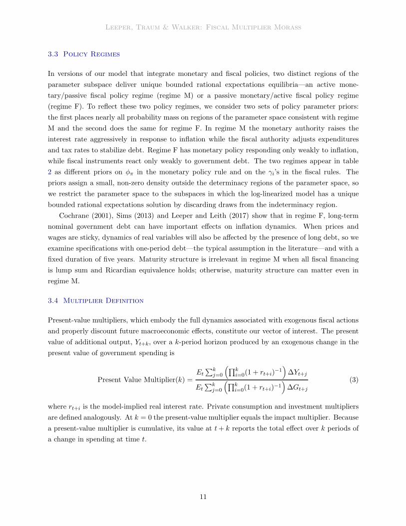
3.4 Multiplier Definition
Present-value multipliers, which embody the full dynamics associated with exogenous fiscal actions
and properly discount future macroeconomic effects, constitute our vector of interest. The present
value of additional output, Yt+k, over a k-period horizon produced by an exogenous change in the
present value of government spending is
Present Value Multiplier(k) =Et∑k
j=0
(
∏ki=0(1 + rt+i)
−1)
∆Yt+j
Et∑k
j=0
(
∏ki=0(1 + rt+i)−1
)
∆Gt+j(3)
where rt+i is the model-implied real interest rate. Private consumption and investment multipliers
are defined analogously. At k = 0 the present-value multiplier equals the impact multiplier. Because
a present-value multiplier is cumulative, its value at t+ k reports the total effect over k periods of
a change in spending at time t.
11
Leeper, Traum & Walker: Fiscal Multiplier Morass
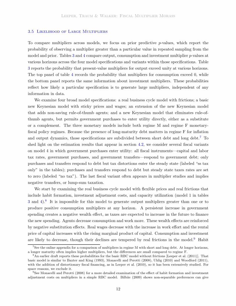
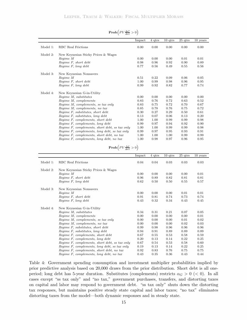
3.5 Likelihood of Large Multipliers
To compare multipliers across models, we focus on prior predictive p-values, which report the
probability of observing a multiplier greater than a particular value in repeated sampling from the
model and prior. Tables 3 and 4 compare output, consumption and investment multiplier p-values at
various horizons across the four model specifications and variants within those specifications. Table
3 reports the probability that present-value multipliers for output exceed unity at various horizons.
The top panel of table 4 records the probability that multipliers for consumption exceed 0, while
the bottom panel reports the same information about investment multipliers. These probabilities
reflect how likely a particular specification is to generate large multipliers, independent of any
information in data.
We examine four broad model specifications: a real business cycle model with frictions; a basic
new Keynesian model with sticky prices and wages; an extension of the new Keynesian model
that adds non-saving rule-of-thumb agents; and a new Keynesian model that eliminates rule-of-
thumb agents, but permits government purchases to enter utility directly, either as a substitute
or a complement. The three monetary models include both regime M and regime F monetary-
fiscal policy regimes. Because the presence of long-maturity debt matters in regime F for inflation
and output dynamics, those specifications are subdivided between short debt and long debt.7 To
shed light on the estimation results that appear in section 4.2, we consider several fiscal variants
on model 4 in which government purchases enter utility: all fiscal instruments—capital and labor
tax rates, government purchases, and government transfers—respond to government debt; only
purchases and transfers respond to debt but tax distortions enter the steady state (labeled “ss tax
only” in the tables); purchases and transfers respond to debt but steady state taxes rates are set
to zero (labeled “no tax”). The last fiscal variant often appears in multiplier studies and implies
negative transfers, or lump-sum taxation.
We start by examining the real business cycle model with flexible prices and real frictions that
include habit formation, investment adjustment costs, and capacity utilization (model 1 in tables
3 and 4).8 It is impossible for this model to generate output multipliers greater than one or to
produce positive consumption multipliers at any horizon. A persistent increase in government
spending creates a negative wealth effect, as taxes are expected to increase in the future to finance
the new spending. Agents decrease consumption and work more. These wealth effects are reinforced
by negative substitution effects. Real wages decrease with the increase in work effort and the rental
price of capital increases with the rising marginal product of capital. Consumption and investment
are likely to decrease, though their declines are tempered by real frictions in the model.9 Habit
7See the online appendix for a comparison of multipliers in regime M with short and long debt. At longer horizons,a longer maturity often implies higher multipliers, but the differences are small compared to regime F.
8An earlier draft reports these probabilities for the basic RBC model without frictions [Leeper et al. (2011)]. Thatbasic model is similar to Baxter and King (1993), Monacelli and Perotti (2008), Uhlig (2010) and Woodford (2011),with the addition of distortionary fiscal financing, as in Leeper et al. (2010), so it has been extensively studied. Forspace reasons, we exclude it.
9See Monacelli and Perotti (2008) for a more detailed examination of the effect of habit formation and investmentadjustment costs on multipliers in a simple RBC model. Bilbiie (2009) shows non-separable preferences can give
12
Leeper, Traum & Walker: Fiscal Multiplier Morass
Prob(
PV ∆Y∆G
> 1)
Impact 4 qtrs 10 qtrs 25 qtrs 10 years
Model 1: RBC Real Frictions 0.00 0.00 0.00 0.00 0.00
Model 2: New Keynesian Sticky Prices & WagesRegime M 0.12 0.01 0.00 0.01 0.01Regime F, short debt 1.00 0.98 0.94 0.92 0.92Regime F, long debt 0.96 0.79 0.68 0.68 0.68
Model 3: New Keynesian NonsaversRegime M 0.59 0.22 0.06 0.04 0.04Regime F, short debt 1.00 1.00 0.97 0.95 0.94Regime F, long debt 1.00 0.94 0.81 0.77 0.76
Model 4: New Keynesian G-in-UtilityRegime M, substitutes 0.00 0.00 0.00 0.00 0.00Regime M, complements 0.84 0.69 0.49 0.31 0.25Regime M, complements, ss tax only 0.84 0.69 0.54 0.47 0.47Regime M, complements, no tax 0.86 0.72 0.56 0.51 0.52Regime F, substitutes, short debt 0.43 0.48 0.66 0.79 0.81Regime F, substitutes, long debt 0.23 0.18 0.21 0.39 0.45Regime F, complements, short debt 1.00 1.00 1.00 0.98 0.97Regime F, complements, long debt 1.00 0.98 0.93 0.89 0.88Regime F, complements, short debt, ss tax only 1.00 1.00 0.99 0.97 0.97Regime F, complements, long debt, ss tax only 1.00 0.98 0.93 0.89 0.86Regime F, complements, short debt, no tax 1.00 1.00 0.99 0.99 0.98Regime F, complements, long debt, no tax 1.00 0.99 0.95 0.93 0.92
Table 3: Government spending output multiplier probabilities implied by prior predictive analysisbased on 20,000 draws from the prior distribution. Short debt is all one-period; long debt has 5-yearduration. Substitutes (complements) restricts αG > 0 (< 0). In all cases except “ss tax only” and“no tax,” government purchases, transfers, and distorting taxes on capital and labor may respondto government debt. “ss tax only” shuts down the distorting tax responses, but maintains positivesteady state capital and labor taxes; “no tax” eliminates distorting taxes from the model—bothdynamic responses and in steady state.
formation makes agents less willing to decrease consumption quickly as changes in consumption are
costly. Investment adjustment costs and capacity utilization costs deter large swings in investment,
offsetting some of the potential crowding out of investment. Despite these tempering forces, declines
in private demand offset most of the increased public demand, causing output to increase by less
than the increase in government consumption.
There is only a small probability that investment will increase at most horizons. This result is
consistent across all regime M specifications, except in the short run when government purchases
enter utility as substitutes for private consumption, as in model 4 in the bottom panel of table 4.
Apart from that exception, any possibility of higher investment stems from a subset of very high
draws for ρG, the serial correlation of government spending. As ρG approaches one, agents view an
exogenous change in government spending as approximately permanent. Permanent increases in
government consumption encourage households to save more, raising investment. This difference
positive consumption multipliers but require consumption to be an inferior good. Feve et al. (2011) shows that amodel with a labor externality can give positive consumption multipliers. Finn (1998) discusses how private andpublic consumption complementarity affect consumption in a RBC model.
13
Leeper, Traum & Walker: Fiscal Multiplier Morass
between permanent and temporary changes to public expenditures echoes earlier work, such as
Aiyagari et al. (1992) and Baxter and King (1993). In the absence of a near-unity value of ρG or
sufficiently strong substitution of purchases for consumption, investment would never rise in regime
M.
Model 2 introduces sticky prices and sticky wages, which increase output multipliers at all
horizons, as Woodford (2011) shows analytically. Greater price stickiness means that more firms
respond to higher government spending by increasing production rather than prices, so markups
respond more strongly. Although the likelihood of large multipliers tapers off over time, in the long
run there continues to be some small probability of sizeable multipliers in regime M. RBC models
cannot produce these positive long-run multipliers; nominal rigidities are necessary for spending
increases to persistently raise output.
Non-savers (model 3) raise fiscal multipliers substantially, a point that Galı et al. (2007), Furlan-
etto (2011), and Colciago (2011) emphasize. In this model, the fraction of non-savers is the most
influential parameter for the output multiplier, as variations in this parameter are necessary to get
mean impact output multipliers greater than one in regime M. Unlike savers, non-savers ignore the
wealth effects of future taxes and consume their entire income each period. If wages are sticky,
then real wages rise with government spending, increasing non-savers’ consumption. With enough
non-savers in the economy, the increase in non-saver consumption can be large enough to cause
total consumption to increase on impact.10 Both the output and consumption effects in regime M
are short-lived, with most of the increase in multipliers disappearing after two years.
In regime M, permitting government spending to enter utility can consistently generate large
multipliers, even in the long run (model 4). The effect is direct: when government purchases
substitute for private consumption, higher purchases raise output, crowd out consumption and
increase investment; when purchases complement consumption, output and consumption multipli-
ers are likely to be large and fairly persistent.11 Higher consumption comes at the cost of lower
investment. The preference parameter that determines the elasticity of substitution between gov-
ernment and private consumption, αG, is by far the most important parameter for determining the
magnitude of multipliers within a given policy regime.
Across all model specifications, the monetary-fiscal policy regime is the dominant factor in
determining government spending impacts: output, consumption and investment multipliers are
far more likely to be large in regime F than in regime M. Long-term debt reduces the probability
of large multipliers in regime F, compared to when all debt is one-period. For example, even when
αG is restricted to being positive, so government spending substitutes for private consumption,
there is a substantial probability of sizeable output and consumption multipliers in regime F; those
probabilities are 0 in regime M. Long-term debt cuts those probabilities in regime F by factors of
10Alternatively, Bilbiie (2011) and Monacelli and Perotti (2008) suggest non-separability in preferences over con-sumption and leisure also can produce positive consumption multipliers, as can deep habits, as shown by Ravn et al.(2006). Devereux et al. (1996) show an externality in production also can give large output responses.
11Models with public spending in the utility function have a long history, see for example Barro (1981), Aschauer(1985), Christiano and Eichenbaum (1992), McGrattan (1994), Finn (1998), and Linnemann and Schabert (2004).
14
Leeper, Traum & Walker: Fiscal Multiplier Morass
Prob(
PV ∆C∆G
> 0)
Impact 4 qtrs 10 qtrs 25 qtrs 10 years
Model 1: RBC Real Frictions 0.00 0.00 0.00 0.00 0.00
Model 2: New Keynesian Sticky Prices & WagesRegime M 0.00 0.00 0.00 0.01 0.01Regime F, short debt 0.98 0.96 0.92 0.90 0.89Regime F, long debt 0.77 0.56 0.49 0.55 0.56
Model 3: New Keynesian NonsaversRegime M 0.51 0.22 0.09 0.06 0.05Regime F, short debt 1.00 0.99 0.98 0.96 0.95Regime F, long debt 0.99 0.92 0.82 0.77 0.74
Model 4: New Keynesian G-in-UtilityRegime M, substitutes 0.00 0.00 0.00 0.00 0.00Regime M, complements 0.83 0.76 0.72 0.63 0.52Regime M, complements, ss tax only 0.83 0.75 0.72 0.70 0.67Regime M, complements, no tax 0.85 0.78 0.76 0.75 0.72Regime F, substitutes, short debt 0.30 0.27 0.29 0.50 0.61Regime F, substitutes, long debt 0.13 0.07 0.06 0.13 0.20Regime F, complements, short debt 1.00 1.00 0.99 0.99 0.98Regime F, complements, long debt 0.99 0.97 0.94 0.92 0.90Regime F, complements, short debt, ss tax only 1.00 1.00 0.99 0.99 0.98Regime F, complements, long debt, ss tax only 0.99 0.97 0.95 0.93 0.91Regime F, complements, short debt, no tax 1.00 1.00 1.00 0.99 0.99Regime F, complements, long debt, no tax 1.00 0.98 0.97 0.96 0.95
Prob(
PV ∆I∆G
> 0)
Impact 4 qtrs 10 qtrs 25 qtrs 10 years
Model 1: RBC Real Frictions 0.04 0.04 0.03 0.03 0.03
Model 2: New Keynesian Sticky Prices & WagesRegime M 0.00 0.00 0.00 0.00 0.01Regime F, short debt 0.96 0.89 0.82 0.81 0.81Regime F, long debt 0.62 0.50 0.50 0.55 0.57
Model 3: New Keynesian NonsaversRegime M 0.00 0.00 0.00 0.01 0.01Regime F, short debt 0.91 0.81 0.74 0.73 0.74Regime F, long debt 0.43 0.32 0.34 0.43 0.45
Model 4: New Keynesian G-in-UtilityRegime M, substitutes 0.34 0.31 0.21 0.07 0.05Regime M, complements 0.00 0.00 0.00 0.00 0.01Regime M, complements, ss tax only 0.00 0.00 0.00 0.01 0.02Regime M, complements, no tax 0.00 0.00 0.00 0.02 0.03Regime F, substitutes, short debt 0.99 0.98 0.96 0.96 0.96Regime F, substitutes, long debt 0.94 0.91 0.89 0.89 0.89Regime F, complements, short debt 0.67 0.55 0.53 0.58 0.59Regime F, complements, long debt 0.20 0.13 0.14 0.22 0.25Regime F, complements, short debt, ss tax only 0.67 0.54 0.53 0.58 0.60Regime F, complements, long debt, ss tax only 0.19 0.13 0.14 0.22 0.25Regime F, complements, short debt, no tax 0.92 0.83 0.76 0.75 0.75Regime F, complements, long debt, no tax 0.43 0.35 0.36 0.43 0.44
Table 4: Government spending consumption and investment multiplier probabilities implied byprior predictive analysis based on 20,000 draws from the prior distribution. Short debt is all one-period; long debt has 5-year duration. Substitutes (complements) restricts αG > 0 (< 0). In allcases except “ss tax only” and “no tax,” government purchases, transfers, and distorting taxeson capital and labor may respond to government debt. “ss tax only” shuts down the distortingtax responses, but maintains positive steady state capital and labor taxes; “no tax” eliminatesdistorting taxes from the model—both dynamic responses and in steady state.
15
Leeper, Traum & Walker: Fiscal Multiplier Morass
between 2 and 5.
Similar patterns emerge in models 2 (sticky prices and wages) and 3 (rule-of-thumb agents).
Moving from regime M to regime F dramatically increases output and consumption multipliers at
all horizons. While the likelihood of large multipliers with non-saving agents in regime M tapers off
sharply beyond horizons of four quarters, in regime F the tapering off is barely discernible. Once
again, though, long debt systematically reduces the probability of realizing large multipliers.
In regime F, large consumption multipliers do not come at the expense of lower investment, as is
true in regime M. All regime F specifications produce a high probability of positive investment mul-
tipliers along with positive consumption effects. The least likely specifications to generate positive
investment impacts combine two factors: government and private consumption are complements
and distorting taxes are present, either in steady state or dynamically responding to increases in
debt. Even in those cases, positive investment effects occur in about 20 percent of the parameter
draws in regime F. Eliminating steady-state taxes increases the likelihood of large multipliers for
all three variables.
3.6 Prior Predictive for Model Selection
Rule-of-thumb agents are prevalent in models of government spending multipliers. Models that
include a sufficiently large fraction of such agents are likely to produce sizeable output and con-
sumption multipliers in the short run in both policy regimes, as tables 3 and 4 show.12 In contrast,
when government spending enters utility, both a broader range and a larger persistence of mul-
tipliers are possible, depending on whether the spending substitutes for or complements private
consumption. This information gleaned from the prior predictive helps to select a model specifica-
tion with which to confront data.
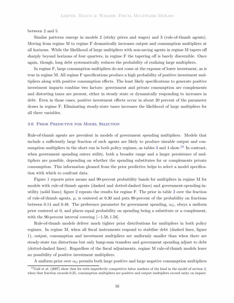
Figure 1 reports prior means and 90-percent probability bands for multipliers in regime M for
models with rule-of-thumb agents (dashed and dotted-dashed lines) and government-spending-in-
utility (solid lines); figure 2 repeats the results for regime F. The prior in table 2 over the fraction
of rule-of-thumb agents, µ, is centered at 0.30 and puts 90-percent of the probability on fractions
between 0.14 and 0.48. The preference parameter for government spending, αG, obeys a uniform
prior centered at 0, and places equal probability on spending being a substitute or a complement,
with the 90-percent interval covering [−1.58, 1.58].
Rule-of-thumb models deliver much tighter prior distributions for multipliers in both policy
regimes. In regime M, when all fiscal instruments respond to stabilize debt (dashed lines, figure
1), output, consumption and investment multipliers are uniformly smaller than when there are
steady-state tax distortions but only lump-sum transfers and government spending adjust to debt
(dotted-dashed lines). Regardless of the fiscal adjustments, regime M rule-of-thumb models leave
no possibility of positive investment multipliers.
A uniform prior over αG permits both large positive and large negative consumption multipliers
12Galı et al. (2007) show that for with imperfectly competitive labor markets of the kind in the model of section 2,when that fraction exceeds 0.25, consumption multipliers are positive and output multipliers exceed unity on impact.
16
Leeper, Traum & Walker: Fiscal Multiplier Morass
0 10 20 30 40
−0.5
0
0.5
1
1.5
2
(a) Output Multiplier
0 10 20 30 40
−1.5
−1
−0.5
0
0.5
1
(b) Consumption Multiplier
0 10 20 30 40
−0.6
−0.5
−0.4
−0.3
−0.2
−0.1
0
0.1
(c) Investment Multiplier
Figure 1: Present-value government spending multipliers in regime M for output, consumptionand investment at various horizons with 90-percent probability bands. Government spending inutility unrestricted, steady-state taxes only, long debt (solid lines); rule-of-thumb agents, everythingresponds to debt, long debt (dashed lines); rule-of-thumb agents, steady-state taxes only, long debt(dotted-dashed lines).
(solid lines), which rule-of-thumb agents preclude. Although most probability mass is on negative
investment effects, this specification does offer some chance for small positive investment multipliers.
Government spending in utility can also generate more persistence in multipliers.
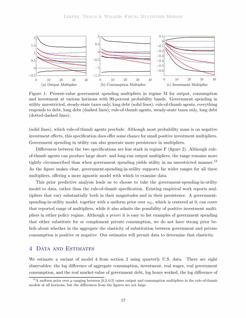
Differences between the two specifications are less stark in regime F (figure 2). Although rule-
of-thumb agents can produce large short- and long-run output multipliers, the range remains more
tightly circumscribed than when government spending yields utility in an unrestricted manner.13
As the figure makes clear, government-spending-in-utility supports far wider ranges for all three
multipliers, offering a more agnostic model with which to examine data.
This prior predictive analysis leads us to choose to take the government-spending-in-utility
model to data, rather than the rule-of-thumb specification. Existing empirical work reports mul-
tipliers that vary substantially both in their magnitudes and in their persistence. A government-
spending-in-utility model, together with a uniform prior over αG, which is centered at 0, can cover
that reported range of multipliers, while it also admits the possibility of positive investment multi-
pliers in either policy regime. Although a priori it is easy to list examples of government spending
that either substitute for or complement private consumption, we do not have strong prior be-
liefs about whether in the aggregate the elasticity of substitution between government and private
consumption is positive or negative. Our estimates will permit data to determine that elasticity.
4 Data and Estimates
We estimate a variant of model 4 from section 2 using quarterly U.S. data. There are eight
observables: the log difference of aggregate consumption, investment, real wages, real government
consumption, and the real market-value of government debt, log hours worked, the log difference of
13A uniform prior over µ ranging between [0.2, 0.5] raises output and consumption multipliers in the rule-of-thumbmodels at all horizons, but the differences from the figures are not large.
17
Leeper, Traum & Walker: Fiscal Multiplier Morass
0 10 20 30 40
0
0.5
1
1.5
2
2.5
(a) Output Multiplier
0 10 20 30 40
−1
−0.5
0
0.5
1
1.5
(b) Consumption Multiplier
0 10 20 30 40
−0.4
−0.2
0
0.2
0.4
(c) Investment Multiplier
Figure 2: Present-value government spending multipliers in regime F for output, consumptionand investment at various horizons with 90-percent probability bands. Government spending inutility unrestricted, steady-state taxes only, long debt (solid lines); rule-of-thumb agents, everythingresponds to debt, long debt (dashed lines); rule-of-thumb agents, steady-state taxes only, long debt(dotted-dashed lines).
the GDP deflator, and the Federal Funds rate. Data are neither detrended nor demeaned. Details
of the data construction and linkage to observables are given in the online appendix. The sample
period is 1955q1 to 2014q2, but we also estimate over two sub-samples: the pre-Volcker era, 1955q1
to 1979q4 and the Great Moderation, 1982q1 to 2007q4. To further investigate the sensitivity of
results to specific sub-samples, we conduct rolling window estimation. The first rolling window
sample consists of 100 quarters from 1955q1 to 1979q4, and consecutively increases the start and
end date by four quarters until the end of our data, with the last sample estimated from 1989q1 to
2013q4.
Our dataset differs from the conventional ones used to estimate new Keynesian models [for
example, Christiano et al. (2005) or Smets and Wouters (2007)] because it includes government debt
and government consumption. Given the question at hand, these are natural additions, but they
change the structure of the data in important ways. Fiscal data typically have more persistence than
other macro aggregates, particularly the market value of government debt. By adding government
debt, our data have more prominent lower frequency variation, so slightly larger than usual frictions
are likely to improve the fit of the data.
4.1 Methodology
We use Bayesian methods to construct the parameters’ posterior distribution, which is a combi-
nation of our priors and the likelihood function, calculated using the Kalman filter. The model
eliminates rule-of-thumb agents and restricts µ = 0. We also do not include tax revenues or
tax rates in the observables and restrict the model so that only public consumption and trans-
fers potentially respond to debt. Tax distortions enter only the steady state, which restricts
γK = γL = ρK = ρL = 0.14 The remaining parameters have either the priors listed in table 2
14We do not include tax rates as observables because quarterly measures of marginal tax rates are problematic.Jones’s (2002) average labor tax rate is not marginal and it exhibits a trend in certain sub-samples. Effective tax rates
18
Leeper, Traum & Walker: Fiscal Multiplier Morass
or the dogmatic priors discussed in section 3.2. As in the prior predictive with long debt, we as-
sume a five-year duration for government bonds. We estimate subject to a monetary-fiscal regime
prior. For regime M, we further restrict the parameters ρZ and ρez. Since transfers are non-
distortionary in regime M, ρZ , ρez, and σZ cannot be separately identified. We restrict ρZ = 0.98
and ρez = 0.8.15 Finally, the investment-specific, price and wage markup shocks are normalized to
enter with a unit coefficient in the investment, price and wage inflation equations respectively.
We take 1.5 million draws from the posterior distribution using the random walk Metropolis-
Hastings algorithm. For purposes of inference, we discard the first 500,000 draws and keep one
every 50 draws to remove some correlation of the draws and obtain a sample from the posterior
equal to our prior sample of 20,000.16
4.2 Posterior Estimates
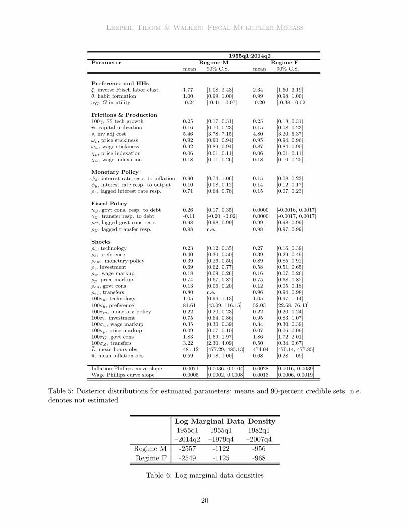
Table 5 reports the posterior estimates for the entire sample 1955q1–2014q2 for regimes M and
F. The online appendix contains parameter estimates for other sub-periods. Three aspects of the
estimates are critical for inferences. First, despite the diffuse priors, the credible sets indicate tight
posteriors for nearly all parameters and across both regimes. Diffuse priors preserve agnosticism
with respect to the multipliers. But data are sufficiently informative to push the posterior distri-
butions into much tighter regions of the parameter space to deliver tightly estimated multipliers.
Second, the posterior means and credible sets are roughly in line with the values reported in the
literature. Public and private consumption are estimated to be complements, as in Bouakez and
Rebei (2007) and Feve et al. (2013). Parameters governing nominal rigidities are slightly larger
than those in Smets and Wouters (2007), but consistent with values reported in Del Negro and
Schorfheide (2008) and Herbst and Schorfheide (2014), who note that higher values in the wage
and price stickiness parameters arise from more diffuse priors. Relatively high degrees of stickiness
make the inflation and wage Phillips curves quite flat. Our estimates of habit formation are high,
but they are within the 90th percentile bands of macro studies of external habits that Havranek,
Rusnak, and Sokolova’s (2015) meta study reports.
Finally, table 6 reports the log marginal data densities for both regimes, and for the entire
sample and subsamples. Log marginal data densities are calculated using Geweke’s (1999) modified
harmonic mean estimator with a truncation parameter of 0.5. The data do not systematically prefer
one regime over the other, so our analysis gives equal weight to the two regimes.17
calculated with alternative procedures, for instance Mendoza et al. (1994), give annual rates that require assumptionsfor interpolating quarterly values.
15In regime M, combinations of high (low) AR(1) coefficients and low (high) standard deviations are similar. Thecalibration for ρZ and ρez was based on estimates from regime F and estimates in regime M with the high AR(1)coefficient and low standard deviation combination. Having AR(1) coefficients in both policy rules and policy shocksare essential in regime F to match features of the data.
16We set the step size to target an acceptance rate in the range of 20 to 40 percent across all cases. Diagnosticsto determine chain convergence include cumulative sum of the draws (CUMSUM) statistics and Geweke’s SeparatedPartial Means (GSPM) test. See the online appendix for more details.
17In contrast to Tan (2014) and Traum and Yang (2011), we find regime F is preferred by the data over someperiods, particularly 1955q1–2014q2. This difference stems from elements of our model in regime F that help the
19
Leeper, Traum & Walker: Fiscal Multiplier Morass
1955q1:2014q2Parameter Regime M Regime F
mean 90% C.S. mean 90% C.S.
Preference and HHsξ, inverse Frisch labor elast. 1.77 [1.08, 2.43] 2.34 [1.50, 3.19]θ, habit formation 1.00 [0.99, 1.00] 0.99 [0.98, 1.00]αG, G in utility -0.24 [-0.41, -0.07] -0.20 [-0.38, -0.02]
Frictions & Production100γ, SS tech growth 0.25 [0.17, 0.31] 0.25 [0.18, 0.31]ψ, capital utilization 0.16 [0.10, 0.23] 0.15 [0.08, 0.23]s, inv adj cost 5.46 [3.78, 7.15] 4.80 [3.20, 6.37]ωp, price stickiness 0.92 [0.90, 0.94] 0.95 [0.94, 0.96]ωw, wage stickiness 0.92 [0.89, 0.94] 0.87 [0.84, 0.90]χp, price indexation 0.06 [0.01, 0.11] 0.06 [0.01, 0.11]χw, wage indexation 0.18 [0.11, 0.26] 0.18 [0.10, 0.25]
Monetary Policyφπ, interest rate resp. to inflation 0.90 [0.74, 1.06] 0.15 [0.08, 0.23]φy, interest rate resp. to output 0.10 [0.08, 0.12] 0.14 [0.12, 0.17]ρr , lagged interest rate resp. 0.71 [0.64, 0.78] 0.15 [0.07, 0.23]
Fiscal PolicyγG, govt cons. resp. to debt 0.26 [0.17, 0.35] 0.0000 [-0.0016, 0.0017]γZ , transfer resp. to debt -0.11 [-0.20, -0.02] 0.0000 [-0.0017, 0.0017]ρG, lagged govt cons resp. 0.98 [0.98, 0.99] 0.99 [0.98, 0.99]ρZ , lagged transfer resp. 0.98 n.e. 0.98 [0.97, 0.99]
Shocksρa, technology 0.23 [0.12, 0.35] 0.27 [0.16, 0.39]ρb, preference 0.40 [0.30, 0.50] 0.39 [0.29, 0.49]ρem, monetary policy 0.39 [0.26, 0.50] 0.89 [0.85, 0.92]ρi, investment 0.69 [0.62, 0.77] 0.58 [0.51, 0.65]ρw, wage markup 0.18 [0.09, 0.26] 0.16 [0.07, 0.26]ρp, price markup 0.74 [0.67, 0.82] 0.75 [0.68, 0.82]ρeg , govt cons 0.13 [0.06, 0.20] 0.12 [0.05, 0.18]ρez , transfers 0.80 n.e. 0.96 [0.94, 0.98]100σa, technology 1.05 [0.96, 1.13] 1.05 [0.97, 1.14]100σb, preference 81.61 [43.09, 116.15] 52.03 [22.68, 76.43]100σm, monetary policy 0.22 [0.20, 0.23] 0.22 [0.20, 0.24]100σi, investment 0.75 [0.64, 0.86] 0.95 [0.83, 1.07]100σw , wage markup 0.35 [0.30, 0.39] 0.34 [0.30, 0.39]100σp, price markup 0.09 [0.07, 0.10] 0.07 [0.06, 0.09]100σG, govt cons 1.83 [1.69, 1.97] 1.86 [1.72, 2.01]100σZ , transfers 3.22 [2.30, 4.09] 0.50 [0.34, 0.67]L, mean hours obs 481.12 [477.29, 485.13] 474.04 [470.14, 477.85]π, mean inflation obs 0.59 [0.18, 1.00] 0.68 [0.28, 1.09]
Inflation Phillips curve slope 0.0071 [0.0036, 0.0104] 0.0028 [0.0016, 0.0039]Wage Phillips curve slope 0.0005 [0.0002, 0.0008] 0.0013 [0.0006, 0.0019]
Table 5: Posterior distributions for estimated parameters: means and 90-percent credible sets. n.e.denotes not estimated
Log Marginal Data Density
1955q1 1955q1 1982q1–2014q2 –1979q4 –2007q4
Regime M -2557 -1122 -956Regime F -2549 -1125 -968
Table 6: Log marginal data densities
20
Leeper, Traum & Walker: Fiscal Multiplier Morass
5 Multipliers
Government spending multipliers are complex objects that depend on every aspect of a model’s
specification. Our estimates reveal some obvious aspects: the presence and degree of nominal and
real rigidities; the role that government spending plays as a complement or substitute for pri-
vate consumption; the stance of monetary and fiscal policies, which encompasses the sources of
fiscal financing and the prevailing monetary-fiscal policy regime. But more subtle aspects of the
model specification also emerge as important for determining multipliers: the absence or presence
of steady-state distorting taxes; the level of steady-state government debt; and the maturity struc-
ture of outstanding debt. Both sets of aspects affect the transmission mechanism of government
spending.
To understand the economic mechanisms that underlie our estimates of multipliers, we present
results in several parts. We begin with an overview of similarities and differences in estimated
responses to a government spending increase across the two policy regimes and then turn to dis-
cussions of the transmission mechanisms, first in regime M, then in regime F. Because differences
in labor market behavior account for much of the variation in government spending effects in the
two regimes, we discuss these differences in detail. Finally, fiscal financing of government spending
differs markedly between regimes, so we end with an analysis of the sources of financing. In all re-
sults, government spending initially rises by 1 percent of steady-state government purchases, which
is calibrated to be 11 percent of model GDP, in line with the average over the estimation period.
5.1 Overview of Multipliers Across Policy Regimes
Tables 7 and 8 summarize present-value multipliers for output, consumption and investment from
the prior predictive and posterior estimates over three sample periods: the full sample, 1955q1–
2014q2; the pre-Volcker period, 1955q1–1979q4; the post-Volcker pre-crisis period, 1982q1–2007q4.
The tables report mean values and 90-percent credible sets for multipliers at selected horizons. Prior
predictive analysis produces very wide ranges for possible multipliers, suggesting that a priori the
model is agnostic about both the magnitudes and signs of government spending effects. Data are
extremely informative about multipliers: posterior credible sets are substantially narrower than the
prior sets and in many cases leave little ambiguity about government spending impacts.
Table 7 reports that in regime M posterior mean estimates of output multipliers are positive
at all horizons and quite likely to be greater than 1 in the short run, but well below 1 over longer
periods. These multipliers are larger over the full sample, which includes the 2008 crisis, than over
either shorter sub-samples.18 This pattern carries over to consumption multipliers: positive in the
short run and at all horizons over the full sample, but zero or even negative at longer horizons
model match features of the data, such as the inclusion of long-term debt and steady-state tax rates. See section5.3 for more discussion. Tan (2014) finds the minimal econometric approach, which elicits priors from a simpler newKeynesian model, can change regime rankings.
18Ramey (2011) reviews the theoretical and empirical literature and concludes that the output multiplier is between0.8 and 1.5, in line with our impact estimates in both regimes.
21
Leeper, Traum & Walker: Fiscal Multiplier Morass
in the 1955–1979 and 1982–2007 sub-periods. Higher government spending unambiguously crowds
out private investment in regime M: at all horizons and sub-periods, the 90-percent credible sets for
investment multipliers are strongly negative even though the prior predictive places some probability
on positive investment multipliers.
Output Multiplier: PV ∆Y∆G
Impact 4 qtrs 10 qtrs 25 qtrs 10 years
Prior 0.80 0.67 0.56 0.50 0.49[-0.58,2.12] [-0.48,1.77] [-0.38,1.55] [-0.39,1.49] [-0.41,1.53]
Posterior1955q1–2014q2 1.36 1.16 0.90 0.70 0.70
[1.17,1.55] [0.99,1.34] [0.72,1.09] [0.48,0.91] [0.45,0.94]1955q1–1979q4 1.41 1.06 0.67 0.41 0.36
[1.15,1.68] [0.84,1.28] [0.50,0.83] [0.29,0.53] [0.24,0.47]1982q1–2007q4 1.26 1.02 0.68 0.39 0.33
[1.03,1.48] [0.82,1.22] [0.50,0.86] [0.22,0.57] [0.13,0.54]
Consumption Multiplier: PV ∆C∆G
Impact 4 qtrs 10 qtrs 25 qtrs 10 years
Prior -0.22 -0.29 -0.33 -0.36 -0.39[-1.53,1.02] [-1.45,0.83] [-1.44,0.73] [-1.40,0.71] [-1.41,0.66]
Posterior1955q1–2014q2 0.24 0.23 0.23 0.23 0.23
[0.07,0.40] [0.06,0.40] [0.06,0.39] [0.06,0.40] [0.06,0.41]1955q1–1979q4 0.45 0.36 0.22 0.03 -0.10
[0.19,0.69] [0.12,0.59] [-0.00,0.44] [-0.18,0.23] [-0.29,0.11]1982q1–2007q4 0.20 0.15 0.05 -0.09 -0.18
[-0.01,0.41] [-0.07,0.36] [-0.17,0.29] [-0.34,0.16] [-0.42,0.07]
Investment Multiplier: PV ∆I∆G
Impact 4 qtrs 10 qtrs 25 qtrs 10 years
Prior -0.06 -0.11 -0.18 -0.23 -0.24[-0.17,0.05] [-0.31,0.07] [-0.51,0.13] [-0.68,0.17] [-0.71,0.20]
Posterior1955q1–2014q2 -0.15 -0.31 -0.56 -0.90 -1.11
[-0.19,-0.10] [-0.40,-0.22] [-0.72,-0.41] [-1.13,-0.66] [-1.42,-0.80]1955q1–1979q4 -0.31 -0.51 -0.75 -0.92 -1.00
[-0.42,-0.20] [-0.65,-0.37] [-0.92,-0.55] [-1.18,-0.66] [-1.33,-0.68]1982q1–2007q4 -0.15 -0.30 -0.52 -0.75 -0.84
[-0.20,-0.10] [-0.40,-0.20] [-0.70,-0.34] [-1.06,-0.45] [-1.24,-0.44]
Table 7: Prior versus posterior mean multipliers for regime M. 90-percent credible sets in brackets.
Regime F multipliers appear in table 8. Unlike regime M, now the prior suggests that positive
output multipliers are nearly certain over longer horizons. For the 1955–2014 sample period, mean
estimates of output multipliers are more than twice the size in regime M: at 10 years, the 90-
percent set in F is [1.65, 2.09], whereas it is [0.45, 0.94] in M. Starker differences emerge in estimates
from the two sub-periods, where the longer-run output multipliers are three to four times larger
in F. Consumption multipliers over the three sample periods are comparable across the regimes,
but marginally more likely to be positive in F. Investment impacts also display regime differences:
22
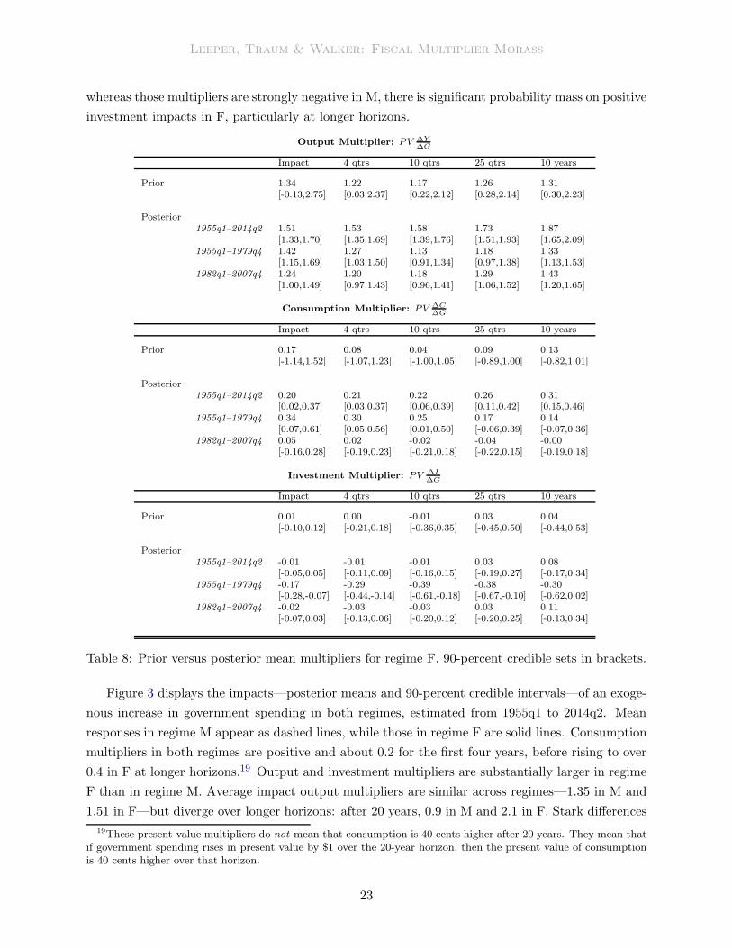
Leeper, Traum & Walker: Fiscal Multiplier Morass
whereas those multipliers are strongly negative in M, there is significant probability mass on positive
investment impacts in F, particularly at longer horizons.
Output Multiplier: PV ∆Y∆G
Impact 4 qtrs 10 qtrs 25 qtrs 10 years
Prior 1.34 1.22 1.17 1.26 1.31[-0.13,2.75] [0.03,2.37] [0.22,2.12] [0.28,2.14] [0.30,2.23]
Posterior1955q1–2014q2 1.51 1.53 1.58 1.73 1.87
[1.33,1.70] [1.35,1.69] [1.39,1.76] [1.51,1.93] [1.65,2.09]1955q1–1979q4 1.42 1.27 1.13 1.18 1.33
[1.15,1.69] [1.03,1.50] [0.91,1.34] [0.97,1.38] [1.13,1.53]1982q1–2007q4 1.24 1.20 1.18 1.29 1.43
[1.00,1.49] [0.97,1.43] [0.96,1.41] [1.06,1.52] [1.20,1.65]
Consumption Multiplier: PV ∆C∆G
Impact 4 qtrs 10 qtrs 25 qtrs 10 years
Prior 0.17 0.08 0.04 0.09 0.13[-1.14,1.52] [-1.07,1.23] [-1.00,1.05] [-0.89,1.00] [-0.82,1.01]
Posterior1955q1–2014q2 0.20 0.21 0.22 0.26 0.31
[0.02,0.37] [0.03,0.37] [0.06,0.39] [0.11,0.42] [0.15,0.46]1955q1–1979q4 0.34 0.30 0.25 0.17 0.14
[0.07,0.61] [0.05,0.56] [0.01,0.50] [-0.06,0.39] [-0.07,0.36]1982q1–2007q4 0.05 0.02 -0.02 -0.04 -0.00
[-0.16,0.28] [-0.19,0.23] [-0.21,0.18] [-0.22,0.15] [-0.19,0.18]
Investment Multiplier: PV ∆I∆G
Impact 4 qtrs 10 qtrs 25 qtrs 10 years
Prior 0.01 0.00 -0.01 0.03 0.04[-0.10,0.12] [-0.21,0.18] [-0.36,0.35] [-0.45,0.50] [-0.44,0.53]
Posterior1955q1–2014q2 -0.01 -0.01 -0.01 0.03 0.08
[-0.05,0.05] [-0.11,0.09] [-0.16,0.15] [-0.19,0.27] [-0.17,0.34]1955q1–1979q4 -0.17 -0.29 -0.39 -0.38 -0.30
[-0.28,-0.07] [-0.44,-0.14] [-0.61,-0.18] [-0.67,-0.10] [-0.62,0.02]1982q1–2007q4 -0.02 -0.03 -0.03 0.03 0.11
[-0.07,0.03] [-0.13,0.06] [-0.20,0.12] [-0.20,0.25] [-0.13,0.34]
Table 8: Prior versus posterior mean multipliers for regime F. 90-percent credible sets in brackets.
Figure 3 displays the impacts—posterior means and 90-percent credible intervals—of an exoge-
nous increase in government spending in both regimes, estimated from 1955q1 to 2014q2. Mean
responses in regime M appear as dashed lines, while those in regime F are solid lines. Consumption
multipliers in both regimes are positive and about 0.2 for the first four years, before rising to over
0.4 in F at longer horizons.19 Output and investment multipliers are substantially larger in regime
F than in regime M. Average impact output multipliers are similar across regimes—1.35 in M and
1.51 in F—but diverge over longer horizons: after 20 years, 0.9 in M and 2.1 in F. Stark differences
19These present-value multipliers do not mean that consumption is 40 cents higher after 20 years. They mean thatif government spending rises in present value by $1 over the 20-year horizon, then the present value of consumptionis 40 cents higher over that horizon.
23
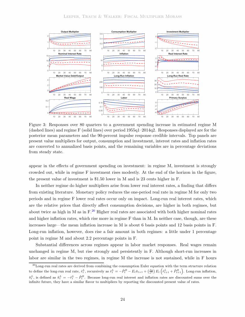
Leeper, Traum & Walker: Fiscal Multiplier Morass
10 20 30 40 50 60 70 80
0
1
2
Output Multiplier
10 20 30 40 50 60 70 80
0
0.2
0.4
0.6
Consumption Multiplier
10 20 30 40 50 60 70 80
-2
-1
0
Investment Multiplier
10 20 30 40 50 60 70 80
0
5
10
15
Nominal Interest Rate
10 20 30 40 50 60 70 80
0
5
10
Inflation
10 20 30 40 50 60 70 80
-4
-2
0
2
Real Interest Rate
10 20 30 40 50 60 70 80
0
2
4
Market Value Debt/Output
10 20 30 40 50 60 70 80
0
100
200
Long-Run Inflation
10 20 30 40 50 60 70 80
0
10
20
30
Long-Run Real Rate
10 20 30 40 50 60 70 80
0
0.1
0.2
Real Wage
10 20 30 40 50 60 70 80
0
0.05
0.1
0.15
Labor
10 20 30 40 50 60 70 80
-6
-4
-2
0
Primary Surplus
Figure 3: Responses over 80 quarters to a government spending increase in estimated regime M(dashed lines) and regime F (solid lines) over period 1955q1–2014q2. Responses displayed are for theposterior mean parameters and the 90-percent impulse response credible intervals. Top panels arepresent value multipliers for output, consumption and investment, interest rates and inflation ratesare converted to annualized basis points, and the remaining variables are in percentage deviationsfrom steady state.
appear in the effects of government spending on investment: in regime M, investment is strongly
crowded out, while in regime F investment rises modestly. At the end of the horizon in the figure,
the present value of investment is $1.50 lower in M and is 23 cents higher in F.
In neither regime do higher multipliers arise from lower real interest rates, a finding that differs
from existing literature. Monetary policy reduces the one-period real rate in regime M for only two
periods and in regime F lower real rates occur only on impact. Long-run real interest rates, which
are the relative prices that directly affect consumption decisions, are higher in both regimes, but
about twice as high in M as in F.20 Higher real rates are associated with both higher nominal rates
and higher inflation rates, which rise more in regime F than in M. In neither case, though, are these
increases large—the mean inflation increase in M is about 6 basis points and 12 basis points in F.
Long-run inflation, however, does rise a fair amount in both regimes: a little under 1 percentage
point in regime M and about 2.2 percentage points in F.
Substantial differences across regimes appear in labor market responses. Real wages remain
unchanged in regime M, but rise strongly and persistently in F. Although short-run increases in
labor are similar in the two regimes, in regime M the increase is not sustained, while in F hours
20Long-run real rates are derived from combining the consumption Euler equation with the term structure relation
to define the long-run real rate, rLt , recursively as rLt = −PBt −Etπt+1 +(
βρ
eγ
)
Et(
rLt+1 + PBt+1
)
. Long-run inflation,
πLt , is defined as πLt = −rLt − PBt . Because long-run real interest and inflation rates are discounted sums over theinfinite future, they have a similar flavor to multipliers by reporting the discounted present value of rates.
24

Leeper, Traum & Walker: Fiscal Multiplier Morass
0 100 200 300 400 500 600 700 800 900 1000−1
0
1
2
3
4
5
6
(a) Market Value of Debt / Output
0 100 200 300 400 500 600 700 800 900 1000−8
−6
−4
−2
0
2
4
6
8
(b) Primary Surplus
Figure 4: Responses of debt and primary surplus to a government spending increase in estimatedregime M (dashed lines) and regime F (solid lines) over period 1955q1–2014q2. Responses displayedare for the posterior mean parameters and variables are in percentage deviations from steady state.
worked remain high over the 20-year period in the figure. These differences, which section 5.4
dissects, highlight how the transmission mechanisms vary across regimes.
In both regimes, the fiscal expansion initially lowers the market value of debt as a share of output
because both output rises and bond prices fall. The very different sources of fiscal financing in the
two regimes appear in figure 4, which reports fiscal responses over 1000 periods to reveal the model’s
low-frequency dynamics. The transition to the initial steady state is extremely slow, echoing Chung
and Leeper’s (2007) VAR evidence. In regime M estimates, fiscal policy raises transfers and reduces
government purchases in response to higher debt, while in regime F those responses are muted.
Both regimes have tax revenues rise passively with capital, labor and consumption increases. A
critical difference in financing comes from the spending reversals that regime M triggers. These
reversals raise surpluses and the value of debt more than in F, but then cause debt to overshoot
the steady state to generate low-frequency oscillations around steady state. Oscillating government
spending produces oscillations in other variables that are absent from regime F, where long-run
convergence to steady state is monotonic.
We now dig more deeply into the transmission mechanisms in the two regimes to better under-
stand the crucial differences that appear in figure 3: multipliers are larger in regime F than in M,
especially over the long run; variables are substantially more persistent in F than in M.
5.2 Transmission Mechanism in Regime M
Regime M combines active monetary policy with passive fiscal policy. Estimates of fiscal behavior,
however, differ somewhat from canonical new Keynesian models that assume lump-sum taxes are
the passive instrument that stabilizes debt. In the 1955q1–2014q2 estimates, government spending
25
Leeper, Traum & Walker: Fiscal Multiplier Morass
is the stabilizing instrument: estimates have spending fall as the debt-output ratio rises, while
lump-sum transfers move perversely and rise as debt rises. The estimated “spending reversals,”
in Corsetti, Meier and Muller’s (2012) terminology, play a key role in regime M’s transmission
mechanism.
5.2.1 Important Parameters To shed light on the transmission mechanisms that under-
lie the estimated multipliers, we calculate a measure of root mean square deviation (RMSD)
for each parameter. For each draw of the posterior parameters, θ = [θ1 ... θn]′ from the
posterior distribution p(θ), we calculate multipliers ω(θ). Denote the new parameter vector by
θi = [θ1 ... E[θi] ... θn]′, where E[θi] fixes the i
th parameter at its posterior mean, and calcu-
late the multipliers, ωi(θi). Repeat this for each i = 1, 2, . . . n. The RMSD is the root mean square
deviation between the two multipliers ω(θ) and ωi(θi): it measures how much the multiplier varies
on average due to parameter i. The RMSD is largest for the parameters that are most influential
for the multiplier.
Table 9 displays the top five parameters by the RMSD ranking, as well as their total contribution
to RMSD variation, across a range of estimated model specifications. The table displays results
for output and consumption present-value multipliers on impact and after 25 quarters following a
government spending shock. Most of the parameters that RMSD calculations identify as important
for output and consumption multipliers fall into three categories: preferences (αG, the coefficient
on government consumption in utility; θ, the degree of habit formation), nominal rigidities (ωp,
the Calvo parameter for price setting; ωw, the Calvo parameter for wage setting; χp, the degree
of inflation indexation), and policy parameters (φπ and φy, the responses of monetary policy to
inflation and output; γZ and γG, the responses of transfers and government spending to debt in
regime M; ρG and ρeg, the persistence of the government spending shock).
5.2.2 Counterfactuals Based on the rankings in table 9, table 10 reports posterior means
and 90-percent credible sets for impact and 25-quarter multipliers under a variety of counterfactual
parameter settings in regime M. For comparison, the table also displays multipliers in the estimated
model. For each counterfactual, we fix the parameters indicated in the table, and let the remaining
parameters vary over the posterior.21
The persistently positive consumption multipliers in regime M that figure 3 depicts come from
a combination of two estimated parameters: the complementarity of government spending (αG <
0) and strong external habit formation (large θ). With complementarity, the initial increase in
government spending raises private consumption despite higher real interest rates. Strong habits
increase the desire for smooth consumption paths that rise only gradually over time, even as
government spending decays back to steady state. Reducing habit formation, θ = 0.8, or removing
government spending’s complementarity to private consumption, αG = 0, reduces output impacts
and shifts the estimated consumption multipliers from positive to negative or zero. These preference
parameters interact: it is the combination of the two counterfactuals that moves credible sets into
21Results come from the same set of 20,000 draws in all cases. We discard draws that lead to indeterminacy.
26
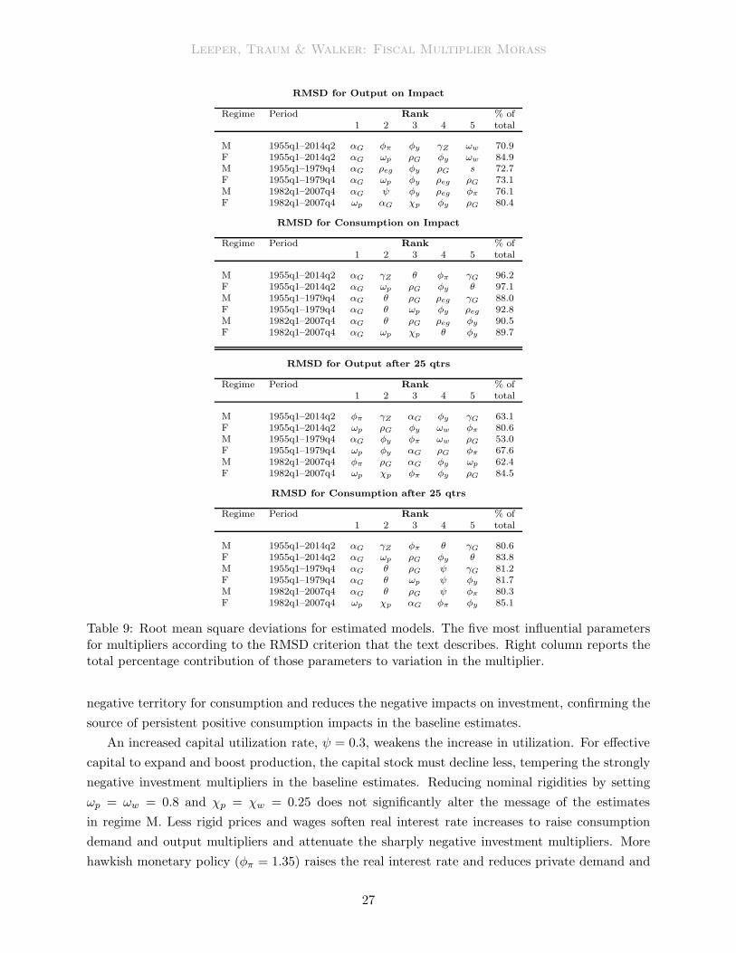
Leeper, Traum & Walker: Fiscal Multiplier Morass
RMSD for Output on Impact
Regime Period Rank % of1 2 3 4 5 total
M 1955q1–2014q2 αG φπ φy γZ ωw 70.9F 1955q1–2014q2 αG ωp ρG φy ωw 84.9M 1955q1–1979q4 αG ρeg φy ρG s 72.7F 1955q1–1979q4 αG ωp φy ρeg ρG 73.1M 1982q1–2007q4 αG ψ φy ρeg φπ 76.1F 1982q1–2007q4 ωp αG χp φy ρG 80.4
RMSD for Consumption on Impact
Regime Period Rank % of1 2 3 4 5 total
M 1955q1–2014q2 αG γZ θ φπ γG 96.2F 1955q1–2014q2 αG ωp ρG φy θ 97.1M 1955q1–1979q4 αG θ ρG ρeg γG 88.0F 1955q1–1979q4 αG θ ωp φy ρeg 92.8M 1982q1–2007q4 αG θ ρG ρeg φy 90.5F 1982q1–2007q4 αG ωp χp θ φy 89.7
RMSD for Output after 25 qtrs
Regime Period Rank % of1 2 3 4 5 total
M 1955q1–2014q2 φπ γZ αG φy γG 63.1F 1955q1–2014q2 ωp ρG φy ωw φπ 80.6M 1955q1–1979q4 αG φy φπ ωw ρG 53.0F 1955q1–1979q4 ωp φy αG ρG φπ 67.6M 1982q1–2007q4 φπ ρG αG φy ωp 62.4F 1982q1–2007q4 ωp χp φπ φy ρG 84.5
RMSD for Consumption after 25 qtrs
Regime Period Rank % of1 2 3 4 5 total
M 1955q1–2014q2 αG γZ φπ θ γG 80.6F 1955q1–2014q2 αG ωp ρG φy θ 83.8M 1955q1–1979q4 αG θ ρG ψ γG 81.2F 1955q1–1979q4 αG θ ωp ψ φy 81.7M 1982q1–2007q4 αG θ ρG ψ φπ 80.3F 1982q1–2007q4 ωp χp αG φπ φy 85.1
Table 9: Root mean square deviations for estimated models. The five most influential parametersfor multipliers according to the RMSD criterion that the text describes. Right column reports thetotal percentage contribution of those parameters to variation in the multiplier.
negative territory for consumption and reduces the negative impacts on investment, confirming the
source of persistent positive consumption impacts in the baseline estimates.
An increased capital utilization rate, ψ = 0.3, weakens the increase in utilization. For effective
capital to expand and boost production, the capital stock must decline less, tempering the strongly
negative investment multipliers in the baseline estimates. Reducing nominal rigidities by setting
ωp = ωw = 0.8 and χp = χw = 0.25 does not significantly alter the message of the estimates
in regime M. Less rigid prices and wages soften real interest rate increases to raise consumption
demand and output multipliers and attenuate the sharply negative investment multipliers. More
hawkish monetary policy (φπ = 1.35) raises the real interest rate and reduces private demand and
27
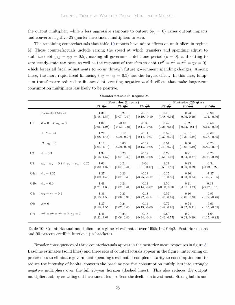
Leeper, Traum & Walker: Fiscal Multiplier Morass
the output multiplier, while a less aggressive response to output (φy = 0) raises output impacts
and converts negative 25-quarter investment multipliers to zero.
The remaining counterfactuals that table 10 reports have minor effects on multipliers in regime
M. Those counterfactuals include raising the speed at which transfers and spending adjust to
stabilize debt (γZ = γG = 0.5), making all government debt one period (ρ = 0), and setting to
zero steady-state tax rates as well as the response of transfers to debt (τK = τL = τC = γZ = 0),
which forces all fiscal adjustments to occur through future government spending changes. Among
these, the more rapid fiscal financing (γZ = γG = 0.5) has the largest effect. In this case, lump-
sum transfers are reduced to finance debt, creating negative wealth effects that make longer-run
consumption multipliers less likely to be positive.
Counterfactuals in Regime M
Posterior (Impact) Posterior (25 qtrs)
PV ∆Y∆G
PV ∆C∆G
PV ∆I∆G
PV ∆Y∆G
PV ∆C∆G
PV ∆I∆G
Estimated Model 1.36 0.24 -0.15 0.70 0.23 -0.90[1.18, 1.55] [0.07, 0.40] [-0.19, -0.10] [0.48, 0.91] [0.06, 0.40] [-1.14, -0.66]
C1: θ = 0.8 & αG = 0 1.02 -0.10 -0.08 0.42 -0.29 -0.50[0.96, 1.08] [-0.13, -0.06] [-0.11, -0.06] [0.26, 0.57] [-0.42, -0.17] [-0.61, -0.38]
A: θ = 0.8 1.26 0.12 -0.11 0.52 -0.13 -0.62[1.08, 1.44] [-0.04, 0.27] [-0.14, -0.07] [0.32, 0.70] [-0.31, 0.05] [-0.78, -0.45]
B: αG = 0 1.10 0.00 -0.12 0.57 0.00 -0.73[1.05, 1.15] [-0.01, 0.00] [-0.15, -0.08] [0.40, 0.75] [-0.05, 0.04] [-0.89, -0.57]
C2: ψ = 0.3 1.34 0.23 -0.12 0.78 0.21 -0.73[1.16, 1.52] [0.07, 0.40] [-0.18, -0.08] [0.54, 1.03] [0.04, 0.37] [-0.98, -0.49]
C3: ωp = ωw = 0.8 & χp = χw = 0.25 1.60 0.24 0.04 1.21 0.23 -0.34[1.32, 1.87] [0.07, 0.41] [-0.13, 0.18] [0.50, 1.86] [0.06, 0.39] [-0.99, 0.27]
C4a: φπ = 1.35 1.27 0.23 -0.21 0.25 0.16 -1.27[1.09, 1.45] [0.07, 0.40] [-0.25, -0.17] [0.13, 0.36] [0.00, 0.34] [-1.49, -1.05]
C4b: φy = 0.0 1.41 0.24 -0.11 1.56 0.21 0.03[1.21, 1.60] [0.07, 0.41] [-0.14, -0.07] [-0.08, 3.10] [-1.11, 1.71] [-0.07, 0.16]
C5: γG = γZ = 0.5 1.31 0.23 -0.18 0.56 0.16 -0.95[1.13, 1.50] [0.00, 0.34] [-0.22, -0.14] [0.44, 0.69] [-0.01, 0.31] [-1.12, -0.78]
C6: ρ = 0 1.37 0.24 -0.14 0.72 0.24 -0.91[1.18, 1.55] [0.07, 0.40] [-0.19, -0.09] [0.49, 0.96] [0.07, 0.41] [-1.15, -0.65]
C7: τK = τL = τC = 0, γZ = 0 1.41 0.23 -0.18 0.60 0.21 -1.04[1.22, 1.61] [0.06, 0.40] [-0.24, -0.14] [0.42, 0.77] [0.05, 0.39] [-1.25, -0.82]
Table 10: Counterfactual multipliers for regime M estimated over 1955q1–2014q2. Posterior meansand 90-percent credible intervals (in brackets).
Broader consequences of three counterfactuals appear in the posterior mean responses in figure 5.
Baseline estimates (solid lines) and three sets of counterfactuals appear in the figure. Intervening on
preferences to eliminate government spending’s estimated complementarity to consumption and to
reduce the intensity of habits, converts the baseline positive consumption multipliers into strongly
negative multipliers over the full 20-year horizon (dashed lines). This also reduces the output
multiplier and, by crowding out investment less, softens the decline in investment. Strong habits and
28
Leeper, Traum & Walker: Fiscal Multiplier Morass
10 20 30 40 50 60 70 80
0
0.5
1
Output Multiplier
10 20 30 40 50 60 70 80
-0.2
0
0.2
Consumption Multiplier
10 20 30 40 50 60 70 80
-2
-1
0
Investment Multiplier
10 20 30 40 50 60 70 80
0
5
10
Nominal Interest Rate
10 20 30 40 50 60 70 80
0
2
4
6
Inflation
10 20 30 40 50 60 70 80
-2
0
2
4
Real Interest Rate
10 20 30 40 50 60 70 80
0
2
4
Market Value Debt
10 20 30 40 50 60 70 80
0
50
100
Long-Run Inflation
10 20 30 40 50 60 70 80
0
20
40
Long-Run Real Rate
10 20 30 40 50 60 70 80
-0.03
-0.02
-0.01
0
Real Wage
10 20 30 40 50 60 70 80
0
0.05
0.1
Labor
10 20 30 40 50 60 70 80
-6
-4
-2
0
Primary Surplus
Figure 5: Counterfactual posterior mean responses to a government spending increase in estimatedregime M, 1955q1–2014q2. Baseline estimates (solid lines); lower habits, θ = 0.8 and no governmentspending in utility, αG = 0 (dashed lines); more aggressive monetary policy, φπ = 1.35 and φy = 0.2(dotted-dashed lines); Ricardian model, γG = 0, γZ = 0.2 (dotted lines). Top panels are presentvalue multipliers for output, consumption and investment, interest rates and inflation rates areconverted to annualized basis points, and the remaining variables are in percentage deviations fromsteady state.
complementary of government spending are essential to deliver the sustained positive consumption
multipliers in the baseline estimates.
More aggressive monetary policy raises nominal and real interest rates after the fiscal expansion,
tempering the increase in inflation for several years (dotted-dashed lines). Sharply higher real rates
reduce consumption multipliers relative to baseline estimates and dramatically lower investment.
A reduced capital stock, together with substantially lower wages and short-lived labor increases,
drive the present-value output multiplier to near zero at longer horizons.
The last counterfactual makes regime M Ricardian in the sense that only non-distorting trans-
fers respond to debt; spending reversals that arise through the rule for government purchases are
eliminated (dotted lines).22 Ricardian fiscal financing coincides with analyses in Christiano et al.
(2011) and Cogan et al. (2010) and other multiplier studies. It produces smaller output multipliers
than the estimated baseline, with consumption multipliers that turn negative after 10 years. These
effects stem from somewhat higher real interest rates and much lower wages.
22“Ricardian” refers only to the sources of financing that respond to the state of government debt. Some revenueis raised through (constant) steady-state tax rates on capital, labor and consumption.
29
Leeper, Traum & Walker: Fiscal Multiplier Morass
5.3 Transmission Mechanism in Regime F
Regime F couples passive monetary policy with active fiscal policy, a policy mix that breaks Ricar-
dian equivalence. Debt-financed government spending does not trigger expectations of sufficiently
high surpluses to stabilize debt. Instead, changes in bond prices and the price level ensure that
the market value of debt is aligned with the expected present value of surpluses. Unlike simple
expositions of this policy regime, the estimated model includes constant tax rates levied against
capital and labor income and consumption, so a fiscal expansion does generate expectations of
somewhat higher surpluses; those surpluses, though, are not a marginal source of financing and
cannot stabilize debt.
Counterfactuals in Regime F
Posterior (Impact) Posterior (25 qtrs)
PV ∆Y∆G
PV ∆C∆G
PV ∆I∆G
PV ∆Y∆G
PV ∆C∆G
PV ∆I∆G
Estimated Model 1.51 0.20 -0.01 1.73 0.26 0.03[1.33, 1.70] [0.02, 0.37] [-0.05, 0.05] [1.51, 1.93] [0.11, 0.42] [-0.19, 0.27]
C1: θ = 0.8 & αG = 0 1.32 0.04 0.01 1.64 0.19 0.05[1.24, 1.40] [-0.01, 0.09] [-0.03, 0.04] [1.41, 1.87] [0.01, 0.36] [-0.11, 0.21]
A: θ = 0.8 1.49 0.20 -0.01 1.67 0.26 -0.01[1.32, 1.67] [0.05, 0.34] [-0.05, 0.03] [1.43, 1.88] [0.07, 0.45] [-0.20, 0.17]
B: αG = 0 1.31 0.01 0.03 1.67 0.10 0.18[1.25, 1.36] [0.00, 0.02] [-0.01, 0.07] [1.47, 1.88] [0.05, 0.16] [0.01, 0.35]
C2: ψ = 0.3 1.49 0.20 0.02 1.78 0.25 0.18[1.31, 1.68] [0.03, 0.38] [-0.03, 0.07] [1.57, 1.99] [0.09, 0.40] [-0.01, 0.38]
C3: ωp = ωw = 0.8 & χp = χw = 0.25 2.30 0.24 0.57 3.91 0.51 2.19[1.99, 2.60] [0.06, 0.41] [0.39, 0.76] [3.21, 4.57] [0.30, 0.71] [1.53, 2.84]
C4a: φπ = 0.225, ρr = 0.71 1.56 0.21 0.03 1.74 0.27 0.05[1.38, 1.76] [0.04, 0.38] [-0.02, 0.08] [1.52, 1.95] [0.11, 0.42] [-0.19, 0.28]
C4b: φy = 0.0 2.60 0.25 0.79 6.19 0.67 4.24[2.24, 2.96] [0.07, 0.43] [0.58, 0.99] [5.13, 7.26] [0.42, 0.92] [3.22, 5.25]
C6: ρ = 0 1.56 0.21 0.03 1.95 0.31 0.18[1.37, 1.75] [0.04, 0.39] [-0.03, 0.08] [1.71, 2.19] [0.15, 0.47] [-0.06, 0.42]
C7: τK = τL = τC = 0 3.41 0.34 1.12 9.77 1.56 5.14[2.82, 3.98] [0.14, 0.52] [0.77, 1.43] [7.47, 12.04] [0.96, 2.13] [3.74, 6.52]
Table 11: Counterfactual multipliers for Regime F estimated over 1955q1–2014q2. Posterior meansand 90-percent credible intervals (in brackets).
5.3.1 Important Parameters Table 9 reports the five most important parameters for output
and consumption multipliers in regime F. Important parameters include price and wage sticki-
ness (ωp and ωw), preferences over government spending and habits (αG and θ), monetary policy
reactions to inflation and output (φπ and φy), and the persistence of government spending (ρG).
These RMSD results guide the counterfactual experiments that follow. Missing from the RMSD
analysis is whether changes in steady-state variables matter for multipliers. As table 10’s C6 and
C7 counterfactuals suggest, steady-state changes in average maturity or tax rates have only tiny
effects in regime M. This is not the case in regime F, as section 5.3.2 discusses.
30
Leeper, Traum & Walker: Fiscal Multiplier Morass
5.3.2 Counterfactuals Table 11 repeats for regime F many of the counterfactuals conducted
in table 10 for regime M. Reducing habit intensity (θ = 0.8) and removing government spending’s
complementarity (αG = 0) have much less effect on consumption multipliers in F than in regime M.
The impact multiplier falls from 0.2 to zero, but the 25-quarter multiplier continues to be positive.
Merely setting αG = 0 still reduces the impact consumption multiplier, but it raises the longer-term
investment multiplier from essentially zero to 0.18.
Multipliers are uniformly higher when prices and wages are more flexible, an outcome that is no
mystery in regime F. Less stickiness permits inflation to rise more after the increase in government
spending which, when monetary policy is passive, reduces real interest rates in the short run.23
Lower real rates raise consumption and investment demand at the same time that they raise supply
of labor.
Monetary policy’s reaction to output, φy, becomes quite powerful when nominal rigidities are
strong, as in the baseline estimates. Making monetary policy unresponsive to output (φy = 0) raises
impact multipliers for output and investment, but the largest effects occur at longer horizons: the
output multiplier exceeds six and the investment multiplier is over four at 25 quarters.
Very large multipliers arise when steady-state tax rates are zero. Impact multipliers for output
and investment rise substantially, but the biggest increases appear in longer-run multipliers, which
are several times larger than in baseline estimates. Eliminating steady-state taxes as a source of
revenue produces very large wealth effects in regime F: now an expansion in debt is completely
unbacked by changes in future surpluses, sharply increasing demand now and in the future.24
Figure 6 reports dynamic impacts of a public spending expansion on the baseline posterior mean
estimates (solid lines) and three counterfactuals. Reducing nominal rigidities (dashed lines) makes
the real interest rate the dominant force in the transmission mechanism because inflation, which
rises dramatically on impact, is transformed into sharply lower real rates by the passive monetary
policy in regime F (dashed lines). Lower real rates trigger the typical reactions: households raise
consumption and investment demand, firms with sticky prices increase labor demand to satisfy
production, increasing equilibrium labor. All three multiplier measures are significantly higher
than in the baseline estimates.
Enhanced price and wage flexibility raises the slopes of the inflation and wage Phillips curves
to transmit increased real activity into still higher inflation and wages, with larger adjustments
in both variables in the short run. Bond prices drop precipitously and drive the market value of
debt-output ratio below steady state over the 20-year horizon in the figure. These large initial
impacts are more fleeting because diminished stickiness reduces persistence in many responses,
most notably nominal interest rates, inflation and labor-market variables.
Dramatic effects come from intervening on preference parameters to reduce habit intensity and
eliminate government spending’s complementarity, while also reducing the persistence of govern-
ment spending (dotted-dashed lines). Without complementarity, the short-run consumption mul-
23A similar mechanism is in play when monetary policy confronts the zero lower bound [Christiano et al. (2011)].24This counterfactual brings the model closest to the canonical fiscal theory setting with exogenous primary sur-
pluses, which Dupor and Li (2015) study.
31
Leeper, Traum & Walker: Fiscal Multiplier Morass
10 20 30 40 50 60 70 80
0
2
4
Output Multiplier
10 20 30 40 50 60 70 80
0
0.2
0.4
0.6
Consumption Multiplier
10 20 30 40 50 60 70 80
0
1
2
Investment Multiplier
10 20 30 40 50 60 70 80
0
20
40
Nominal Interest Rate
10 20 30 40 50 60 70 80
0
20
40
60
Inflation
10 20 30 40 50 60 70 80
-40
-20
0
Real Interest Rate
10 20 30 40 50 60 70 80
-2
-1
0
1
Market Value Debt
10 20 30 40 50 60 70 80
0
200
400
600
Long-Run Inflation
10 20 30 40 50 60 70 80
-200
-100
0
Long-Run Real Rate
10 20 30 40 50 60 70 80
0
0.05
0.1
0.15
Real Wage
10 20 30 40 50 60 70 80
0
0.2
0.4
Labor
10 20 30 40 50 60 70 80
-6
-4
-2
0
Primary Surplus
Figure 6: Counterfactual posterior mean responses to a government spending increase in estimatedRegime F, 1955q1–2014q2. Baseline estimates (solid lines); lower nominal rigidities, ωp = ωw = 0.7(dashed lines); lower habits, θ = 0.8, no government spending in utility, αG = 0, and less persistentspending shock, ρG = 0.9 (dotted-dashed lines); lower nominal rigidities, ωp = ωw = 0.7, lowerhabits, θ = 0.8, no government spending in utility, αG = 0, and less persistent spending shock,ρG = 0.9 (dotted lines). Top panels are present value multipliers for output, consumption andinvestment, interest rates and inflation rates are converted to annualized basis points, and theremaining variables are in percentage deviations from steady state.
tiplier can turn negative as real interest rates rise modestly, while weaker habits permit long-run
consumption multipliers to rise to the baseline’s levels, even as the government spending injection
dissipates. Output and investment multipliers also fall below their baseline levels. With a less
sustained increase in demand due to reduced serial correlation in government purchases, labor and
wages rise only tepidly.
The third counterfactual combines the first two to show that complementarity of government
and private consumption and extremely persistent government spending—all of which emerge from
the baseline estimates—are not necessary to generate persistently positive consumption multipliers
in regime F (dotted lines). This scenario generates small, transitory increases in inflation, nominal
interest rates and labor, yet a set of multipliers that is larger than in the baseline.
Persistence in regime F—in contrast to regime M—comes in large part from slowly evolving
government debt. Analytical models of the two regimes make clear that government debt is an
important state variable in F, but disappears in equilibrium in purely Ricardian versions of M.
This role of debt is difficult to glean from the counterfactuals in figure 6, so we now turn to
interventions on features of the steady state that have a direct bearing on the state of government
debt.
Figure 7 reports the baseline responses (solid lines) and responses from interventions on three
32
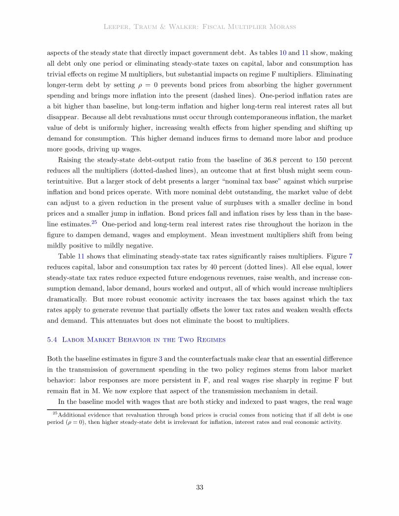
Leeper, Traum & Walker: Fiscal Multiplier Morass
aspects of the steady state that directly impact government debt. As tables 10 and 11 show, making
all debt only one period or eliminating steady-state taxes on capital, labor and consumption has
trivial effects on regime M multipliers, but substantial impacts on regime F multipliers. Eliminating
longer-term debt by setting ρ = 0 prevents bond prices from absorbing the higher government
spending and brings more inflation into the present (dashed lines). One-period inflation rates are
a bit higher than baseline, but long-term inflation and higher long-term real interest rates all but
disappear. Because all debt revaluations must occur through contemporaneous inflation, the market
value of debt is uniformly higher, increasing wealth effects from higher spending and shifting up
demand for consumption. This higher demand induces firms to demand more labor and produce
more goods, driving up wages.
Raising the steady-state debt-output ratio from the baseline of 36.8 percent to 150 percent
reduces all the multipliers (dotted-dashed lines), an outcome that at first blush might seem coun-
terintuitive. But a larger stock of debt presents a larger “nominal tax base” against which surprise
inflation and bond prices operate. With more nominal debt outstanding, the market value of debt
can adjust to a given reduction in the present value of surpluses with a smaller decline in bond
prices and a smaller jump in inflation. Bond prices fall and inflation rises by less than in the base-
line estimates.25 One-period and long-term real interest rates rise throughout the horizon in the
figure to dampen demand, wages and employment. Mean investment multipliers shift from being
mildly positive to mildly negative.
Table 11 shows that eliminating steady-state tax rates significantly raises multipliers. Figure 7
reduces capital, labor and consumption tax rates by 40 percent (dotted lines). All else equal, lower
steady-state tax rates reduce expected future endogenous revenues, raise wealth, and increase con-
sumption demand, labor demand, hours worked and output, all of which would increase multipliers
dramatically. But more robust economic activity increases the tax bases against which the tax
rates apply to generate revenue that partially offsets the lower tax rates and weaken wealth effects
and demand. This attenuates but does not eliminate the boost to multipliers.
5.4 Labor Market Behavior in the Two Regimes
Both the baseline estimates in figure 3 and the counterfactuals make clear that an essential difference
in the transmission of government spending in the two policy regimes stems from labor market
behavior: labor responses are more persistent in F, and real wages rise sharply in regime F but
remain flat in M. We now explore that aspect of the transmission mechanism in detail.
In the baseline model with wages that are both sticky and indexed to past wages, the real wage
25Additional evidence that revaluation through bond prices is crucial comes from noticing that if all debt is oneperiod (ρ = 0), then higher steady-state debt is irrelevant for inflation, interest rates and real economic activity.
33
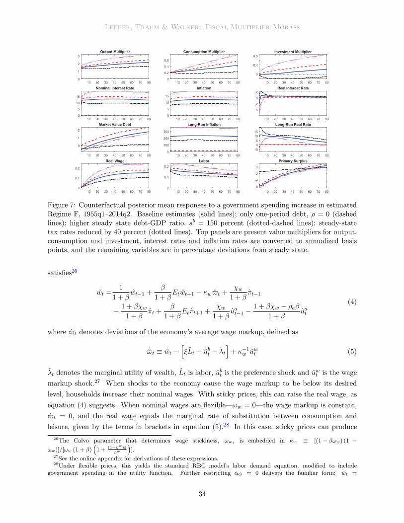
Leeper, Traum & Walker: Fiscal Multiplier Morass
10 20 30 40 50 60 70 80
0
1
2
3
Output Multiplier
10 20 30 40 50 60 70 80
0
0.2
0.4
0.6
Consumption Multiplier
10 20 30 40 50 60 70 80
0
0.4
0.8
Investment Multiplier
10 20 30 40 50 60 70 80
0
5
10
15
Nominal Interest Rate
10 20 30 40 50 60 70 80
0
5
10
15
Inflation
10 20 30 40 50 60 70 80
-4
-2
0
2
Real Interest Rate
10 20 30 40 50 60 70 80
0
1
2
Market Value Debt
10 20 30 40 50 60 70 80
0
100
200
300
Long-Run Inflation
10 20 30 40 50 60 70 80
-5
0
5
10
15
Long-Run Real Rate
10 20 30 40 50 60 70 80
0
0.1
0.2
Real Wage
10 20 30 40 50 60 70 80
0
0.1
0.2
Labor
10 20 30 40 50 60 70 80
-6
-4
-2
0
Primary Surplus
Figure 7: Counterfactual posterior mean responses to a government spending increase in estimatedRegime F, 1955q1–2014q2. Baseline estimates (solid lines); only one-period debt, ρ = 0 (dashedlines); higher steady state debt-GDP ratio, sb = 150 percent (dotted-dashed lines); steady-statetax rates reduced by 40 percent (dotted lines). Top panels are present value multipliers for output,consumption and investment, interest rates and inflation rates are converted to annualized basispoints, and the remaining variables are in percentage deviations from steady state.
satisfies26
wt =1
1 + βwt−1 +
β
1 + βEtwt+1 − κw ˆ t +
χw1 + β
πt−1
−1 + βχw1 + β
πt +β
1 + βEtπt+1 +
χw1 + β
uat−1 −1 + βχw − ρaβ
1 + βuat
(4)
where ˆ t denotes deviations of the economy’s average wage markup, defined as
ˆ t ≡ wt −[
ξLt + ubt − λt
]
+ κ−1w uwt (5)
λt denotes the marginal utility of wealth, Lt is labor, ubt is the preference shock and uwt is the wage
markup shock.27 When shocks to the economy cause the wage markup to be below its desired
level, households increase their nominal wages. With sticky prices, this can raise the real wage, as
equation (4) suggests. When nominal wages are flexible—ωw = 0—the wage markup is constant,
ˆ t = 0, and the real wage equals the marginal rate of substitution between consumption and
leisure, given by the terms in brackets in equation (5).28 In this case, sticky prices can produce
26The Calvo parameter that determines wage stickiness, ωw, is embedded in κw ≡ [(1− βωw) (1 −
ωw)]/[ωw (1 + β)(
1 + (1+ηw)ξηw
)
].27See the online appendix for derivations of these expressions.28Under flexible prices, this yields the standard RBC model’s labor demand equation, modified to include
government spending in the utility function. Further restricting αG = 0 delivers the familiar form: wt =
34
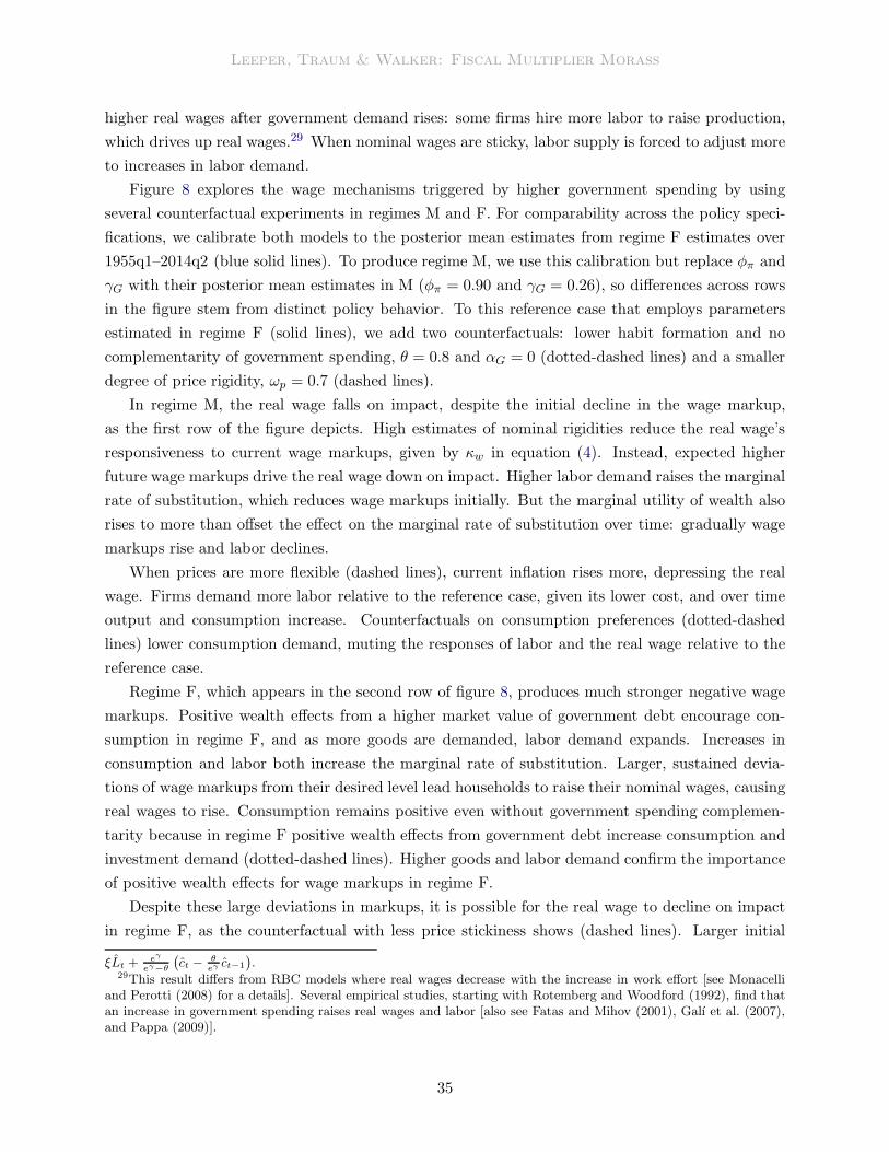
Leeper, Traum & Walker: Fiscal Multiplier Morass
higher real wages after government demand rises: some firms hire more labor to raise production,
which drives up real wages.29 When nominal wages are sticky, labor supply is forced to adjust more
to increases in labor demand.
Figure 8 explores the wage mechanisms triggered by higher government spending by using
several counterfactual experiments in regimes M and F. For comparability across the policy speci-
fications, we calibrate both models to the posterior mean estimates from regime F estimates over
1955q1–2014q2 (blue solid lines). To produce regime M, we use this calibration but replace φπ and
γG with their posterior mean estimates in M (φπ = 0.90 and γG = 0.26), so differences across rows
in the figure stem from distinct policy behavior. To this reference case that employs parameters
estimated in regime F (solid lines), we add two counterfactuals: lower habit formation and no
complementarity of government spending, θ = 0.8 and αG = 0 (dotted-dashed lines) and a smaller
degree of price rigidity, ωp = 0.7 (dashed lines).
In regime M, the real wage falls on impact, despite the initial decline in the wage markup,
as the first row of the figure depicts. High estimates of nominal rigidities reduce the real wage’s
responsiveness to current wage markups, given by κw in equation (4). Instead, expected higher
future wage markups drive the real wage down on impact. Higher labor demand raises the marginal
rate of substitution, which reduces wage markups initially. But the marginal utility of wealth also
rises to more than offset the effect on the marginal rate of substitution over time: gradually wage
markups rise and labor declines.
When prices are more flexible (dashed lines), current inflation rises more, depressing the real
wage. Firms demand more labor relative to the reference case, given its lower cost, and over time
output and consumption increase. Counterfactuals on consumption preferences (dotted-dashed
lines) lower consumption demand, muting the responses of labor and the real wage relative to the
reference case.
Regime F, which appears in the second row of figure 8, produces much stronger negative wage
markups. Positive wealth effects from a higher market value of government debt encourage con-
sumption in regime F, and as more goods are demanded, labor demand expands. Increases in
consumption and labor both increase the marginal rate of substitution. Larger, sustained devia-
tions of wage markups from their desired level lead households to raise their nominal wages, causing
real wages to rise. Consumption remains positive even without government spending complemen-
tarity because in regime F positive wealth effects from government debt increase consumption and
investment demand (dotted-dashed lines). Higher goods and labor demand confirm the importance
of positive wealth effects for wage markups in regime F.
Despite these large deviations in markups, it is possible for the real wage to decline on impact
in regime F, as the counterfactual with less price stickiness shows (dashed lines). Larger initial
ξLt +eγ
eγ−θ
(
ct −θeγ
ct−1
)
.29This result differs from RBC models where real wages decrease with the increase in work effort [see Monacelli
and Perotti (2008) for a details]. Several empirical studies, starting with Rotemberg and Woodford (1992), find thatan increase in government spending raises real wages and labor [also see Fatas and Mihov (2001), Galı et al. (2007),and Pappa (2009)].
35
Leeper, Traum & Walker: Fiscal Multiplier Morass
20 40 60 80
0.4
0.6
0.8
1
1.2
M: Output Multiplier
20 40 60 80
-0.4
-0.3
-0.2
-0.1
0
0.1
M: Consumption Multiplier
20 40 60 80
-0.03
-0.02
-0.01
0
0.01
0.02
0.03
M: Real Wage
20 40 60 80
-0.25
-0.2
-0.15
-0.1
-0.05
0
M: Wage Markup
20 40 60 80
0.02
0.04
0.06
0.08
0.1
0.12
M: Labor
20 40 60 80
1.5
2
2.5
3
3.5
4
F: Output Multiplier
20 40 60 80
0.2
0.4
0.6
0.8
1
1.2
1.4
F: Consumption Multiplier
20 40 60 80
0
0.05
0.1
0.15
F: Real Wage
20 40 60 80
-1.4
-1.2
-1
-0.8
-0.6
-0.4
F: Wage Markup
20 40 60 80
0.15
0.2
0.25
0.3
0.35
0.4
F: Labor
Figure 8: Counterfactual labor market responses to a government spending increase in regime M(top row) and F (bottom row) calibrating both regime using regime F estimates over 1955–2014.Regime M replaces monetary and fiscal parameters with their regime M estimates (φπ = 0.90and γG = 0.26). Reference case (solid lines); reduced habits and eliminating complementarity ofgovernment spending, θ = 0.8 and αG = 0 (dotted-dashed lines); reduced price rigidities, ωp = 0.7(dashed lines).
increases in prices lower the real wage, but strong negative markups make this effect short-lived.
Higher inflation devalues a larger share of government debt, and with more flexible prices, the real
interest rates falls; both effects fuel consumption and further depress wage markups, leading the
real wage to increase over time.
Returning to our baseline posterior estimates in the two regimes that appear in figure 3, dif-
ferences in the effects of government spending on real wages lie at the heart of the differences in
multiplier estimates. Regime F produces larger declines in wage markups, which lead to higher
nominal and real wage adjustments. Coupled with the slightly higher estimated degree of price
stickiness in regime F, which further raises real wages on impact, it is not surprising that real
wages are far more expansive in regime F.
5.5 Fiscal Financing in the Two Regimes
Further insights into the observed differences in multipliers come from accounting for the financing
of government spending increases, which differs across policy regimes and sample periods. Letting
rBt ≡ (βρ/eγ)PBt − PBt−1 − πt denote the ex-post real return on government bonds and St be the
primary surplus, the intertemporal equilibrium condition is30
bt−1 = −βρ
eγPBt + PBt−1 + πt + (1− β)Et
∞∑
j=0
βj St+j − Et
∞∑
j=1
βj rBt+j (6)
30The primary surplus consists of the sum of revenues from capital, labor and consumption taxes less lump-sum
transfers and government purchases: St =TK
S
(
τKt + rKt + Kt
)
+ TL
S
(
τLt + wt + Lt)
+ TC
S
(
τCt + Ct)
−ZSZt−
GSGt.
To focus solely on financing of government purchases, we set all disturbances to zero other than government spending.
36
Leeper, Traum & Walker: Fiscal Multiplier Morass
The model’s rule for government spending at t includes both the exogenous disturbance to
spending, uGt , and an endogenous response of spending to the debt-output ratio, sbt−1, Gt =
ρGGt−1 − γG(1− ρG)sbt−1 + uGt .
We separate government spending into its exogenous, Gxt , and endogenous, Get components,
so Gt = Gxt + Get . Define the effect on the present value of surpluses of an exogenous change in
spending at t by ξt ≡ −(1 − β)GSEt∑∞
j=0 βjGxt+j . We can now split the present value of primary
surpluses following a shock to government spending into exogenous and endogenous parts
(1− β)Et
∞∑
j=0
βj St+j = (1− β)Et
∞∑
j=0
βj [Sxt+j + Set+j] = ξt + (1− β)Et
∞∑
j=0
βj Set+j (7)
where Set is the surplus exclusive of exogenous government spending, Gxt − ρGGxt−1 + uGt .
Substitute (7) into (6) to yield
ξt = bt−1 +βρ
eγPBt − PBt−1 − πt − uGt + Et
∞∑
j=1
βj rBt+j − (1− β)Et
∞∑
j=0
βjSet+j (8)
Table 12 reports the fraction of ξt accounted for by each element in (8) dated t and later,
with endogenous surpluses broken into their component parts. The table includes posterior means
and 90-percent credible sets for the six estimated models, as well as mean predictions for select
counterfactuals. Positive entries in the table mean that the component supports financing of higher
government spending, while negative entries counter financing.
In both regimes, the baseline estimates (1954–2014) imply that a drop in bond prices at the time
of the fiscal shock supports the financing of spending by reducing the market value of debt (PBt
column). Lower PBt alone accounts for 11 percent of the financing in regime M and over 14 percent
in F. By spreading inflation into the future, lower bond prices coincide with contemporaneous
inflation that accounts for less than 1 percent in each regime (πt column). Because the fiscal
expansion raises real interest rates in both M and F, the higher ex-post return on bonds counters
fiscal financing (PV (rB) column), and counters more strongly in M, where real rates rise more.
Important financing differences between regimes emerge from the components of the primary
surplus. Higher tax revenues—the sum of columns PV (TK), PV (TL) and PV (TC)—provide 24
percent of financing in regime M, but nearly 87 percent in F. Under regime M policies, higher
government spending leaves wages unchanged, raises labor moderately, reduces the capital stock,
and raises the return to capital to produce offsetting effects that net out to a modest increase in
tax revenues. Regime F, in contrast, permits higher spending to raise wages and hours worked
dramatically and, if anything, increase the capital stock. This passive, but large, increase in tax
revenues in regime F moderates the wealth effects of fiscal expansions that would otherwise produce
huge multipliers.31
31Tables 10 and 11 show that eliminating these passive revenue adjustments by setting steady-state tax rates tozero has little impact on multipliers in regime M, but raises them significantly in regime F.
37
Leeper, Traum & Walker: Fiscal Multiplier Morass
Of course, if passive tax revenues are not stabilizing debt in regime M, then fiscal adjustments
must be occurring on the expenditures side. Posterior estimates of the response of transfers to debt
in M suggest that transfers actually rise with higher debt [see estimate of γZ in table 5]. In the
accounting exercise, this policy implies that transfers counter the financing of a fiscal expansion.
Financing’s heavy lifting comes from endogenous government spending reversals that rise in present
value by over 113 percent to compensate for the contrary movement in transfers [PV (Z) and
PV (Ge) columns]. This underscores the centrality of government spending reversals in baseline
estimates of regime M. Regime F’s prior is tightly centered on no response of expenditures to debt,
so PV (Z) and PV (Ge) account for less than 0.05 percent of financing.
This general pattern of financing is largely robust across the 1955–1979 and 1982–2007 sub-
periods. One notable difference is that in the earlier sub-period contemporaneous bond prices
play a bigger role in financing in regime F, accounting for nearly a quarter of the expansion in
spending. In the earlier sub-period, both transfers and spending help to stabilize debt in regime
M, so spending reversals are less pronounced and consumption multipliers are smaller.
The counterfactual exercises whose dynamic impacts appear in figures 5 through 7 shift sources
of financing substantially. A Ricardian environment in regime M reduces the role of debt revaluation
through bond prices and current inflation to push nearly all financing into lower future lump-
sum transfers. Reduced habits and removing government spending from utility produces stronger
spending reversals, with PV (Ge) = 130 percent. More aggressive monetary policy shifts more
financing into declines in current bond prices and, by increasing ex-post real returns on debt, raise
debt service to produce a higher path for debt that generates still larger spending reversals. In
these last two cases, large ultimate declines in government purchases make consumption multipliers
higher than they would be in the absence of reversals.
More dramatic reshuffling of fiscal financing appears in regime F counterfactuals. Reduced
nominal stickiness enhances the role of debt revaluations to concentrate more than a third of
financing in current bond prices and inflation. Because less rigidity reduces real interest rates,
ex-post returns on bonds now support the financing of spending. But less expansive real wages and
less persistent labor increases conspire to make endogenous tax revenues less important, cutting
PV (Se) in half.
Removing the maturity structure on government debt also removes any role for drops in bond
prices to support financing. But it also produces larger multipliers and pushes most financing into
endogenous tax revenues that account for 100 percent of the present-value increase in government
spending. Higher steady-state debt-output makes drops in bond prices and surprise inflation more
potent, accounting for 48 percent of financing. The lower associated multipliers reduce the financing
role of steady-state tax rates. Of course, the role of endogenous revenues is also diminished when
steady-state tax rates are reduced 40 percent. With lower future tax revenues, bond prices and
inflation take on larger revaluation roles, as in conventional fiscal theory exercises.
38

Leeper,Traum
&Walker:FiscalMult
iplierMorass
Percentage of Government Spending Financing, ξt, Due to
Specification PBt πt PV (rB) PV (TK) PV (TL) PV (TC) PV (Z) PV (Ge) PV (Se)Posterior Estimates
1955q1–2014q2Regime M 11.1 0.4 -6.3 8.1 14.1 2.0 -42.9 113.5 94.8
[8.2, 13.6] [0.3, 0.6] [-8.7, -3.7] [4.8, 11.6] [8.3, 20.0] [1.1, 2.9] [-78.3, -6.5] [77.9, 149.4] [91.8, 97.7]Regime F 14.4 0.7 -1.7 30.8 53.4 2.5 0.0 0.0 86.8
[11.8, 17.0] [0.5, 0.8] [-3.3, -0.2] [29.6, 32.0] [51.3, 55.5] [1.8, 3.2] [-0.2, 0.2] [-0.2, 0.2] [83.9, 89.7]1955q1–1979q4
Regime M 6.7 0.0 -6.8 1.0 1.7 -0.6 51.6 46.5 100.1[0.7, 12.7] [-0.3, 0.3] [-9.0, -4.5] [-0.7, 2.7] [-1.3, 4.7] [-0.9, -0.3] [30.0, 73.6] [24.9, 66.6] [94.2, 105.7]
Regime F 24.3 0.9 -9.8 30.4 52.7 1.7 0.0 0.0 84.8[18.4, 29.9] [0.6, 1.2] [-14.6, -5.2] [28.6, 32.2] [49.5, 55.8] [1.0, 2.4] [-0.3, 0.3] [-0.4, 0.5] [79.9, 89.6]
1982q1–2007q4Regime M 10.8 0.3 -9.1 4.0 6.9 0.5 -20.9 107.6 98.0
[7.3, 14.2] [0.1, 0.4] [-12.1, -6.1] [0.1, 8.1] [0.1, 14.1] [-0.2, 1.2] [-56.5, 19.4] [69.6, 143.2] [95.3, 100.8]Regime F 17.9 0.4 -5.1 31.1 53.8 2.0 0.0 0.0 86.9
[13.2, 22.9] [0.1, 0.9] [-7.8, -2.5] [29.4, 32.8] [50.9, 56.8] [1.2, 2.8] [-0.3, 0.3] [-0.4, 0.4] [82.2, 91.3]Counterfactuals Based on 1955q1–2014q2 Estimates
Regime MRicardian 3.2 0.0 −6.9 3.4 5.9 −0.9 95.2 0 103.6
θ = 0.8, αG = 0 6.2 0.2 −4.2 5.0 8.6 1.9 −48.1 130.4 97.8φπ = 1.35, φy = 0.2 12.0 0.4 −10.8 1.5 2.6 1.4 −54.3 147.2 98.4
Regime FParameters
ωp = ωw = 0.7 30.9 4.4 18.5 16.4 28.4 1.5 0.0 0.0 46.2θ = 0.8, αG = 0, ρG = 0.9 19.9 0.7 −9.1 31.4 54.3 2.9 0.0 0.0 88.6
ωp = ωw = 0.7 &θ = 0.8, αG = 0, ρG = 0.9 38.6 5.0 8.1 17.0 29.5 1.8 0.0 0.0 48.3
Regime FSteady State
ρ = 0 0 0.8 −0.9 35.5 61.5 3.1 0.0 0.0 100.1sb = 150% 46.0 2.0 −11.7 22.8 39.5 1.4 0.0 0.0 63.7
Lower τ 20.8 1.0 0.2 27.6 47.9 2.5 0.0 0.0 78.0
Table 12: Reports the percentage of ξt accounted for by each element on the right side of equation (8); means and 90-percent credibleintervals (in brackets) of priors and posteriors displayed. Positive entries support financing and negative entries counter financing ofhigher government spending. 0.0 entries represent values < 0.05. Mean rows may not sum to 100 percent due to rounding. Regime M(Ricardian) sets γG = 0 and γZ = 0.2; regime M (θ = 0.8, αG = 0) reduces habit formation and removes government spending fromutility; regime M (απ = 1.35, αy = 0.2) raises monetary policy reactions to inflation and output; regime F (ωp = ωw = 0.5) reduces priceand wage stickiness; regime F (θ = 0.8, αG = 0, ρG = 0.9) reduces habit formation, removes government spending from utility, and makesgovernment spending less persistent; regime F (ωp = ωw = 0.5, θ = 0.8, αG = 0, ρG = 0.9) combines the two previous counterfactuals;regime F (sb = 150%) sets the steady-state ratio of the market value of debt to output at 150 percent; regime F (ρ = 0) makes all debtone period; regime F (lower τ) reduces steady-state tax rates on capital, labor and consumption by 40 percent.
39
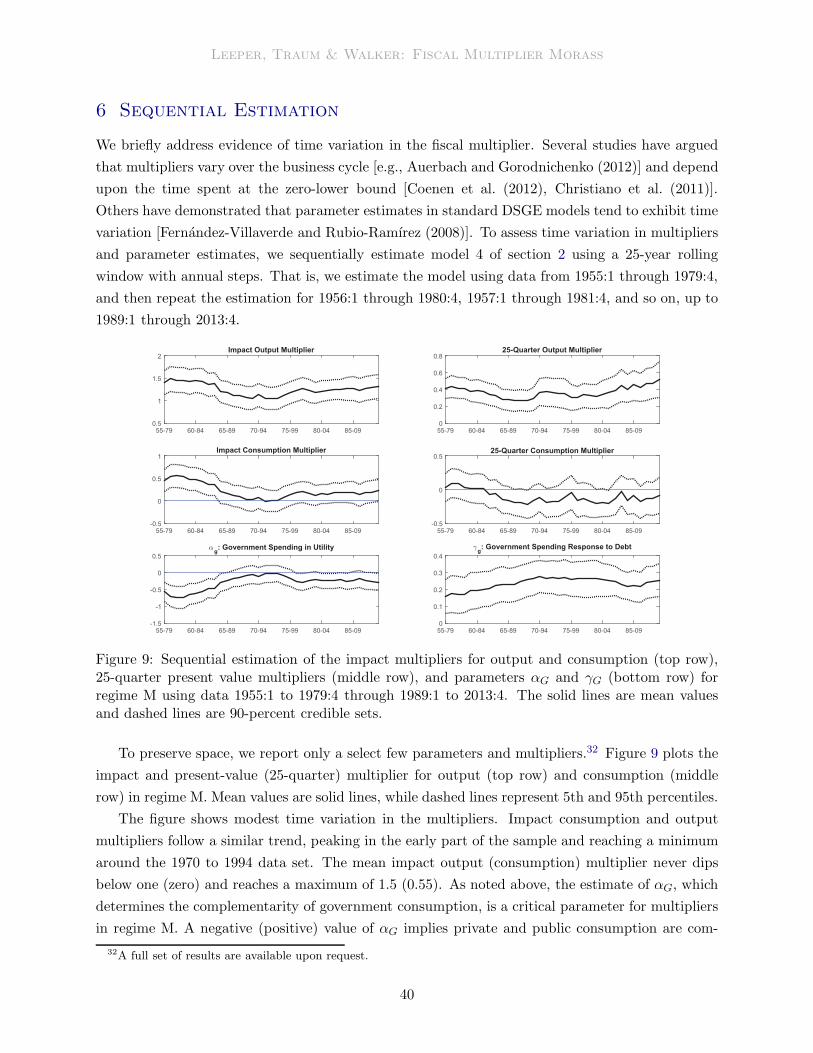
Leeper, Traum & Walker: Fiscal Multiplier Morass
6 Sequential Estimation
We briefly address evidence of time variation in the fiscal multiplier. Several studies have argued
that multipliers vary over the business cycle [e.g., Auerbach and Gorodnichenko (2012)] and depend
upon the time spent at the zero-lower bound [Coenen et al. (2012), Christiano et al. (2011)].
Others have demonstrated that parameter estimates in standard DSGE models tend to exhibit time
variation [Fernandez-Villaverde and Rubio-Ramırez (2008)]. To assess time variation in multipliers
and parameter estimates, we sequentially estimate model 4 of section 2 using a 25-year rolling
window with annual steps. That is, we estimate the model using data from 1955:1 through 1979:4,
and then repeat the estimation for 1956:1 through 1980:4, 1957:1 through 1981:4, and so on, up to
1989:1 through 2013:4.
55-79 60-84 65-89 70-94 75-99 80-04 85-09
0.5
1
1.5
2
Impact Output Multiplier
55-79 60-84 65-89 70-94 75-99 80-04 85-09
0
0.2
0.4
0.6
0.8
25-Quarter Output Multiplier
55-79 60-84 65-89 70-94 75-99 80-04 85-09
-0.5
0
0.5
1
Impact Consumption Multiplier
55-79 60-84 65-89 70-94 75-99 80-04 85-09
-0.5
0
0.525-Quarter Consumption Multiplier
55-79 60-84 65-89 70-94 75-99 80-04 85-09
-1.5
-1
-0.5
0
0.5
αg: Government Spending in Utility
55-79 60-84 65-89 70-94 75-99 80-04 85-09
0
0.1
0.2
0.3
0.4
γg: Government Spending Response to Debt
Figure 9: Sequential estimation of the impact multipliers for output and consumption (top row),25-quarter present value multipliers (middle row), and parameters αG and γG (bottom row) forregime M using data 1955:1 to 1979:4 through 1989:1 to 2013:4. The solid lines are mean valuesand dashed lines are 90-percent credible sets.
To preserve space, we report only a select few parameters and multipliers.32 Figure 9 plots the
impact and present-value (25-quarter) multiplier for output (top row) and consumption (middle
row) in regime M. Mean values are solid lines, while dashed lines represent 5th and 95th percentiles.
The figure shows modest time variation in the multipliers. Impact consumption and output
multipliers follow a similar trend, peaking in the early part of the sample and reaching a minimum
around the 1970 to 1994 data set. The mean impact output (consumption) multiplier never dips
below one (zero) and reaches a maximum of 1.5 (0.55). As noted above, the estimate of αG, which
determines the complementarity of government consumption, is a critical parameter for multipliers
in regime M. A negative (positive) value of αG implies private and public consumption are com-
32A full set of results are available upon request.
40
Leeper, Traum & Walker: Fiscal Multiplier Morass
plements (substitutes). Trends in output and consumption impact multipliers mirror movements
in αG. The early time periods yield a large negative value for αG, where impact multipliers are
largest. Estimates of αG increase over time, reaching a mean value of zero for the 1971 to 1995
data set. This time period coincides with the smallest impact multipliers.
Longer-horizon multipliers exhibit less variation than the impact multipliers. The mean present-
value output multiplier begins around 0.4, dips to roughly 0.3 mid-sample before returning to 0.5
by the end of the sample. The 25-quarter consumption multiplier trends slightly lower for several
periods, and then stabilizes around -0.2 beginning with the 1965 to 1989 sample. Movements in
the 25-quarter multipliers connect to time variation in γG, the strength of spending reversals. This
parameter increases over the same horizon that the consumption multiplier is falling, and both
stabilize around the same time period. Increases in γG bring forth faster spending reversals. At
longer horizons, this makes more goods available to the private sector and increases consumption
multipliers. But in the short run, faster spending reversals lower expected government demand,
muting inflation responses and raising the real interest rate. The higher real interest rate depresses
consumption, explaining the negative relationship between γG and consumption multipliers at the
25-quarter horizon.
Figure 9 underscores the tightness of the estimates for the multipliers and parameters for all
time periods. Recall that the prior predictive range for impact multipliers extends well beyond two
(one) and below zero (-0.5) for output (consumption). The 90-percent posterior credible sets are
much narrower than the prior predictive analysis, indicating that the data are informative.
7 Concluding Remarks
This paper differs from the bulk of research on government spending multipliers in several ways: (1)
expands the set of observables used in estimation; (2) fills out details on the fiscal side of the model,
including explicit rules for fiscal instruments, maturity structure of government debt, government
spending that may complement or substitute for private consumption, distorting steady-state taxes;
(3) adopts more diffuse priors over nominal rigidities and habit formation; (4) permits the posterior
to land in regions of the parameter space that uncover fresh perspectives on the transmission
mechanism of government spending; (6) finds that monetary-fiscal regime is important for the size
and persistence of multipliers: they are larger and more persistent in regime F, but even regime M
estimates produce larger and longer lasting multipliers than most studies.
Our model departs from many others by permitting government spending to enter utility and
allowing data to determine whether public goods substitute for or complement private consump-
tion. This is a crude way to deviate from the common assumption that government spending is
“unproductive” or “wasteful.” More detailed analysis would divide spending into its uses—pure
public goods, national defense, wages of government employees, infrastructure, and so forth—and
aim to model each component. Surely government spending’s impacts hinge on its uses.
The paper highlights an issue that transcends multipliers: getting the prevailing monetary-
fiscal policy regime right is the first order of business for understanding macroeconomic policy
41
Leeper, Traum & Walker: Fiscal Multiplier Morass
impacts. Fiscal details that bring the model closer to actual policy environments matter a great
deal for making regime F dynamics palatable to data. These details, together with other aspects
of model specifications—private sector behavior, the role of government spending, policy rules—
require systematic study to understand their contributions to model fit.
References
Aiyagari, S. R., L. J. Christiano, and M. Eichenbaum (1992): “The Output, Employment,
and Interest Rate Effects of Government Consumption,” Journal of Monetary Economics, 30,
73–86.
Aschauer, D. A. (1985): “Fiscal Policy and Aggregate Demand,” American Economic review,
75.
Auerbach, A. J. and Y. Gorodnichenko (2012): “Measuring the Output Responses to Fiscal
Policy,” American Economic Journal: Economic Policy, 4, 1–27.
Barro, R. J. (1981): “Output Effects of Government Purchases,” Journal of Political Economy,
89, 1086–1121.
Baxter, M. and R. G. King (1993): “Fiscal Policy in General Equilibrium,” American Economic
Review, 86, 1154–1174.
Bilbiie, F. (2009): “Non-Separable Preferences, Fiscal Policy Puzzles and Inferior Goods,” Journal
of Money, Credit and Banking, 41, 443–450.
——— (2011): “Nonseparable Preferences, Frisch Labor Supply, and the Consumption Multiplier
of Government Spending: One Solution to a Fiscal Policy Puzzle,” Journal of Money, Credit and
Banking, 43, 221–251.
Bouakez, H. and N. Rebei (2007): “Why Does Private Consumption Rise After a Government
Spending Shock?” Canadian Journal of Economics, 40, 954–979.
Calvo, G. A. (1983): “Staggered Prices in a Utility Maxmimizing Model,” Journal of Monetary
Economics, 12, 383–398.
Christiano, L., M. Eichenbaum, and S. Rebelo (2011): “When Is the Government Spending
Multiplier Large?” Journal of Political Economy, 119, 78–121.
Christiano, L. J. and M. Eichenbaum (1992): “Current Real-Business-Cycle Theories and
Aggregate Labor-Market Fluctuations,” American Economic Review, 82, 430–450.
Christiano, L. J., M. Eichenbaum, and C. L. Evans (2005): “Nominal Rigidities and the
Dynamic Effects of a Shock to Monetary Policy,” Journal of Political Economy, 113, 1–45.
42
Leeper, Traum & Walker: Fiscal Multiplier Morass
Chung, H. and E. M. Leeper (2007): “What Has Financed Government Debt?” National
Bureau of Economic Research Working Paper No. 13425.
Cochrane, J. H. (1999): “A Frictionless View of U.S. Inflation,” in NBER Macroeconomics
Annual 1998, ed. by B. S. Bernanke and J. J. Rotemberg, Cambridge, MA: MIT Press, vol. 14,
323–384.
——— (2001): “Long Term Debt and Optimal Policy in the Fiscal Theory of the Price Level,”
Econometrica, 69, 69–116.
Coenen, G., C. Erceg, C. Freedman, D. Furceri, M. Kumhof, R. Lalonde, D. Lax-
ton, J. Linde, A. Mourougane, D. Muir, S. Mursula, C. de Resende, J. Roberts,
W. Roeger, S. Snudden, M. Trabandt, and J. in’t Veld (2012): “Effects of Fiscal Stim-
ulus in Structural Models,” American Economic Journal: Macroeconomics, 22–68.
Coenen, G. and R. Straub (2005): “Does Government Spending Crowd In Private Consump-
tion? Theory and Empirical Evidence for the Euro Area,” International Finance, 8, 437–470.
Cogan, J. F., T. Cwik, J. B. Taylor, and V. Wieland (2010): “New Keynesian versus Old
Keynesian Government Spending Multipliers,” Journal of Economic Dynamics and Control, 34,
281–295.
Colciago, A. (2011): “Rule-of-Thumb Consumers Meet Sticky Wages,” Journal of Money, Credit
and Banking, 43, 325–353.
Corsetti, G., A. Meier, and G. Muller (2012): “Fiscal Stimulus with Spending Reversals,”
The Review of Economics and Statistics, 94, 878–895.
Davig, T. and E. M. Leeper (2011): “Monetary-Fiscal Policy Interactions and Fiscal Stimulus,”
European Economic Review, 55, 211–227.
Del Negro, M. and F. Schorfheide (2008): “Forming Priors for DSGE Models (and How It
Affects the Assessment of Nominal Rigidities),” Journal of Monetary Economics, 55, 1191–1208.
Devereux, M. B., A. C. Head, and B. J. Lapham (1996): “Monopolistic Competition, Increas-
ing Returns, and the Effects of Government Spending,” Journal of Money, Credit and Banking,
28, 233–254.
Drautzburg, T. and H. Uhlig (2013): “Fiscal Stimulus and Distortionary Taxes,” Federal
Reserve Bank of Philadelphia, working paper.
Dupor, B. and R. Li (2015): “The Expected Inflation Channel of Government Spending in the
Postwar U.S.” European Economic Review, 74, 36–56.
Erceg, C. J., L. Guerrieri, and C. J. Gust (2006): “SIGMA: A New Open Economy Model
for Policy Analysis,” International Journal of Central Banking, 2.
43
Leeper, Traum & Walker: Fiscal Multiplier Morass
Fatas, A. and I. Mihov (2001): “The Effects of Fiscal Policy on Consumption and Employment:
Theory and Evidence,” Mimeo, INSEAD.
Faust, J. and A. Gupta (2010): “Posterior Predictive Analysis for Evaluating DSGE Models,”
Working Paper, Johns Hopkins University.
Fernandez-Villaverde, J. and J. F. Rubio-Ramırez (2008): “How Structural Are Structural
Parameters?” in NBER Macroeconomics Annual 2007, ed. by D. Acemoglu, K. Rogoff, and
M. Woodford, Chicago, IL: University of Chicago Press, vol. 22.
Feve, P., J. Matheron, and J.-G. Sahuc (2011): “Externality in Labor Supply and Govern-
ment Spending,” Economic Letters, 112, 273–276.
——— (2013): “A Pitfall with Estimated DSGE-Based Government Spending Multipliers,” Amer-
ican Economic Journal: Macroeconomics, 5, 141–178.
Finn, M. G. (1998): “Cyclical Effects of Government’s Employment and Goods Purchases,” In-
ternational Economic Review, 39, 635–657.
Forni, L., L. Monteforte, and L. Sessa (2009): “The General Equilibrium Effects of Fiscal
Policy: Estimates for the Euro Area,” Journal of Public Economics, 93, 559–585.
Furlanetto, F. (2011): “Fiscal Stimulus and the Role of Wage Rigidity,” Journal of Economic
Dynamics and Control, 35, 512–527.
Galı, J., J. D. Lopez-Salido, and J. Valles (2007): “Understanding the Effects of Government
Spending on Consumption,” Journal of the European Economic Association, 5, 227–270.
Gechert, S. and H. Will (2012): “Fiscal Multipliers: A Meta Regression Analysis,” IMK
Working Paper No. 97, July.
Geweke, J. (1999): “Using Simulation Methods for Bayesian Econometric Models: Inference,
Development, and Communication,” Econometric Reviews, 18, 1–73.
——— (2010): Complete and Incomplete Econometric Models, Princeton, NJ: Princeton University
Press.
Havranek, T., M. Rusnak, and A. Sokolova (2015): “Habit Formation in Consumption: A
Meta-Analysis,” Czech National Bank Working Paper No. 2015/03.
Herbst, E. and F. Schorfheide (2014): “Sequential Monte Carlo Sampling for DSGE Models,”
Journal of Applied Econometrics, 29, 1073–1098.
Jones, J. B. (2002): “Has Fiscal Policy Helped Stabilize the Postwar U.S. Economy?” Journal of
Monetary Economics, 49, 709–746.
44
Leeper, Traum & Walker: Fiscal Multiplier Morass
Kim, S. (2003): “Structural Shocks and the Fiscal Theory of the Price Level in the Sticky Price
Model,” Macroeconomic Dynamics, 7, 759–782.
Leeper, E. M. (1991): “Equilibria Under ‘Active’ and ‘Passive’ Monetary and Fiscal Policies,”
Journal of Monetary Economics, 27, 129–147.
Leeper, E. M. and C. Leith (2017): “Inflation Through the Lens of the Fiscal Theory,” in
forthcoming in Handbook of Macroeconomics, ed. by J. B. Taylor and H. Uhlig, Amsterdam:
Elsevier Press, vol. 2.
Leeper, E. M., M. Plante, and N. Traum (2010): “Dynamics of Fiscal Financing in the
United States,” Journal of Econometrics, 156, 304–321.
Leeper, E. M., N. Traum, and T. B. Walker (2011): “Clearing Up the Fiscal Multiplier
Morass,” NBER Working Paper No. 17444, September.
Linnemann, L. and A. Schabert (2004): “Can Fiscal Spending Stimulate Private Consump-
tion?” Economic Letters, 82, 173–179.
Lopez-Salido, J. D. and P. Rabanal (2006): “Government Spending and Consumption-Hours
Preferences,” La Caixa Working Paper Series No. 02/2006, November.
McGrattan, E. R. (1994): “The Macroeconomic Effects of Distortionary Taxation,” Journal of
Monetary Economics, 33, 573–601.
Mendoza, E. G., A. Razin, and L. L. Tesar (1994): “Effective Tax Rates in Macroeconomics
Cross-country Estimates of Tax Rates on Factor Incomes and Consumption,” Journal of Mone-
tary Economics, 34, 297–323.
Monacelli, T. and R. Perotti (2008): “Fiscal Policy, Wealth Effects, and Markups,” National
Bureau of Economic Research Working Paper No. 14584, December.
Pappa, E. (2009): “The Effects of Fiscal Shocks on Employment and the Real Wage,” International
Economic Review, 50, 217–244.
Ramey, V. A. (2011): “Can Government Purchases Stimulate the Economy?” Journal of Eco-
nomic Literature, 49, 673–685.
Ravn, M., S. Schmitt-Grohe, and M. Uribe (2006): “Deep Habits,” Review of Economic
Studies, 73, 195–218.
Rotemberg, J. J. and M. Woodford (1992): “Oligopolistic Pricing and the Effects of Aggregate
Demand on Economic Activity,” Journal of Political Economy, 100, 1153–1207.
Sims, C. A. (1994): “A Simple Model for Study of the Determination of the Price Level and the
Interaction of Monetary and Fiscal Policy,” Economic Theory, 4, 381–399.
45
Leeper, Traum & Walker: Fiscal Multiplier Morass
——— (2013): “Paper Money,” American Economic Review, 103, 563–84.
Smets, F. and R. Wouters (2003): “An Estimated Dynamic Stochastic General Equilibrium
Model of the Euro Area,” Journal of the European Economic Association, 1, 1123–1175.
——— (2005): “Comparing Shocks and Frictions in U.S. and Euro Business Cycles: A Bayesian
DSGE Approach,” Journal of Applied Econometrics, 20, 161–183.
——— (2007): “Shocks and Frictions in US Business Cycles: A Bayesian DSGE Approach,” Amer-
ican Economic Review, 97, 586–606.
Tan, F. (2014): “Two Econometric Interpretations of U.S. Fiscal and Monetary Policy Interac-
tions,” Indiana University manuscript.
Traum, N. and S.-C. S. Yang (2011): “Monetary and Fiscal Policy Interactions in the Post-War
U.S.” European Economic Review, 55, 140–164.
——— (2015): “When Does Government Debt Crowd Out Investment?” Journal of Applied Econo-
metrics, 30, 24–45.
Uhlig, H. (2010): “Some Fiscal Calculus,” American Economic Review: Papers & Proceedings,
100, 30–34.
Woodford, M. (1995): “Price-Level Determinacy Without Control of a Monetary Aggregate,”
Carneige-Rochester Conference Series on Public Policy, 43, 1–46.
——— (2011): “Simple Analytics of the Government Expenditure Multiplier,” American Economic
Journal: Macroeconomics, 3, 1–35.
Zubairy, S. (2014): “On Fiscal Multipliers: Estimates from a Medium-Scale DSGE Model,”
International Economic Review, 55, 169–195.
46


![Microsoft PowerPoint - 2008 08 email morass [Compatibility Mode]](https://img.pdfslide.us/doc/110x75/555272e8b4c905d41d8b56a8/microsoft-powerpoint-2008-08-email-morass-compatibility-mode.jpg)