IZA DP No. 732

Clean Evidence on Peer Pressure

Armin FalkAndrea Ichino

March 2003

DI

SC

US

SI

ON

PA

PE

R S

ER

IE

S

Forschungsinstitutzur Zukunft der ArbeitInstitute for the Studyof Labor

Clean Evidence on Peer Pressure

Armin Falk University of Zurich, CEPR,

CESifo and IZA Bonn

Andrea Ichino European University Institute, CEPR,

CESifo and IZA Bonn

Discussion Paper No. 732 March 2003

IZA

P.O. Box 7240 D-53072 Bonn

Germany

Tel.: +49-228-3894-0 Fax: +49-228-3894-210

Email: iza@iza.org

This Discussion Paper is issued within the framework of IZA’s research area The Future of Labor. Any opinions expressed here are those of the author(s) and not those of the institute. Research disseminated by IZA may include views on policy, but the institute itself takes no institutional policy positions. The Institute for the Study of Labor (IZA) in Bonn is a local and virtual international research center and a place of communication between science, politics and business. IZA is an independent, nonprofit limited liability company (Gesellschaft mit beschränkter Haftung) supported by the Deutsche Post AG. The center is associated with the University of Bonn and offers a stimulating research environment through its research networks, research support, and visitors and doctoral programs. IZA engages in (i) original and internationally competitive research in all fields of labor economics, (ii) development of policy concepts, and (iii) dissemination of research results and concepts to the interested public. The current research program deals with (1) mobility and flexibility of labor, (2) internationalization of labor markets, (3) welfare state and labor market, (4) labor markets in transition countries, (5) the future of labor, (6) evaluation of labor market policies and projects and (7) general labor economics. IZA Discussion Papers often represent preliminary work and are circulated to encourage discussion. Citation of such a paper should account for its provisional character. A revised version may be available on the IZA website (www.iza.org) or directly from the author.

IZA Discussion Paper No. 732 March 2003

ABSTRACT

Clean Evidence on Peer Pressure∗ While confounding factors typically jeopardize the possibility of using observational data to measure peer effects, field experiments over the potential for obtaining clean evidence. In this paper we measure the output of subjects who were asked to stuff letters into envelopes, with a remuneration completely independent of output. We study two treatments. In the "pair" treatment two subjects work at the same time in the same room. Peer effects are possible in this situation and imply that outputs within pairs should be similar. In the "single" treatment, which serves as a control, subjects work alone in a room and peer effects are ruled out by design. Our main results are as follows: First, we find clear and unambiguous evidence for the existence of peer effects in the pair treatment. The standard deviations of output are significantly smaller within pairs than between pairs. Second, average output in the pair treatment largely exceeds output in the single treatment, i.e., peer effects raise productivity. Third, low productivity workers are significantly more sensitive to the behavior of peers than are high productivity workers. Our findings yield important implications for the design of the workplace. JEL Classification: D2, J2, K4 Keywords: peer effects, field experiments, incentives Corresponding author: Armin Falk University of Zurich Institute for Research in Empirical Economics Blumlisalpstr. 10 CH-8006 Zurich Switzerland Tel. +41-1-634 37 04 Email: falk@iew.unizh.ch

∗ We would like to thank Urs Fischbacher, Michel Kosfeld and Gianfranco Pieretti for useful conversations. Jasmin Gülden and Barbara Nabold provided excellent research assistantship.

1 Introduction

Scholars in many disciplines have long tried to estimate empirically the extent

to which individual behavior is modified by peer effects. The reason why

doing this is difficult, despite the apparent wealth of evidence from daily

experience, is that observational data do not allow us to easily separate the

pure effect of peer behavior from the effect of confounding factors. Using

data from a controlled field experiment where randomly selected subjects

were paid independently of their work output, we show in this paper that

the productivity of a worker is systematically influenced by the productivity

of peers in the absence of confounding factors. These results provide clean

evidence for the existence of peer effects on work behavior.

In order to understand the nature of our experiment, consider two indi-

viduals working at separate tasks, where one is in sight of the other. Suppose

that we observe them behaving in a similar way, which we suspect could be

generated by peer effects. To be precise, we say that peer effects exist if the

output of individual i increases when the output of j increases and nothing

else changes. Following Manski [1993], a first set of confounding factors is

generated by the possibility that local attributes of the environments in which

the two individuals operate determine their behavior. If observational data

do not allow us to fully control for these local attributes, we could observe

the behavior of i and j changing simultaneously even in the absence of true

peer effects simply because some unobserved local attributes have changed.

Second, it is possible that the two individuals have similar characteristics,

which would make them behave similarly even if they were not working one

in sight of the other. With respect to both of these possibilities, it could also

happen that i and j decide to work near each other because they like the

2

same local attribute, which in turn affects their behavior, or because they

both like to be near individuals with similar characteristics. In these cases,

the supposed effect of peers would instead be the result of sorting according

to local or personal attributes.

The most recent generation of studies, which try to measure peer effects

with observational data, has made several important steps towards solving

these problems.1 However, even if the setting offers an almost perfect oppor-

tunity to identify peer effects in many of these studies, the impossibility of

controlling for all local or personal confounding factors and for endogenous

sorting makes the identification strategy not fully convincing. The most sig-

nificant recent steps forward in this literature are offered by Sacerdote [2001]

and Katz, Kling and Liebman [2001] who use data based on randomized

assignments of individuals to peer groups. However, both of these papers

are confronted with the consequences of local confounding factors. More

specifically, Sacerdote [2001] finds evidence of peer effects among Dartmouth

students randomly assigned to the same dorm but cannot convincingly ex-

clude the possibility that these effects might be due to local time varying

shocks. This is less of a problem in Katz, Kling and Liebman [2001], who

analyze the consequences of randomly changing the residential neighborhood

of families residing in high-poverty public housing projects and, therefore,

are not primarily interested in isolating pure peer effects from local effects.

A further important difference with respect to our setting is that neither of

these papers focuses on a work environment.

In contrast, we focus explicitly on a real work environment in our study

1See, among others, Wilson [1987], Case and Katz [1991], Crane [1991], Glaeser etal. [1996], Topa [1997], Encinosa et al. [1998], Aaronson [1998], Van Den Berg [1998],Bertrand et al. [2000], Ichino and Maggi [2000], Katz, Kling and Liebman [2001] andSacerdote [2001]. See also the literature based on the classic Hawthorne experiments (e.g.,Whitehead [1938] and more recently Jones [1990]).

3

and we aim to assess the existence of peer effects in a fully controlled setting

where no possible confounding factor can hinder this assessment. As in any

other controlled experiment, the possibility of obtaining clean evidence com-

plements the evidence generated by observational studies in an informative

way.2

Our subjects were recruited randomly and asked to perform a typical

short term job, which was paid independently of individual or team output.

The work task was to stuff letters into envelopes. We study two treatments.

In the ‘pair’ treatment, which is our main treatment, two subjects work

simultaneously in the same room. This setting allows for the possibility that

the behavior of a subject is affected by the behavior of the other member

of the pair. Given two subjects i and j in a pair, we speak of positive peer

effects if the output of i systematically raises the output of j, and vice versa,

leading to similar output levels within the pair. A formal characterization

of this definition will be given in Section 3. In the second treatment (the

‘single’ treatment), which serves as control, peer effects are ruled out by

design because subjects work alone in a room. Output in this treatment

reveals the level of productivity in the absence of any peer influence. The

comparison of the outputs arising in the pair treatment with those from the

single treatment permits the assessment of the effects of peers on individual

productivity.

Our main results are the following: First, we find strong and unambiguous

evidence for the existence of positive peer effects in the pair treatment. This

can be inferred from the fact that output within pairs is very similar, while

2For related literature on laboratory experiments aimed at measuring peer effects seeFalk and Fischbacher [2002] and Falk, Fischbacher, and Gachter [2002]. Nagin et al. [2002]provide instead an example of controlled experimentation in a real labor setting, althoughtheir focus is on a different issue.

4

differing substantially between pairs. This difference is particularly striking

when compared to what happens in random allocations of subjects from the

pair and the single treatment in simulated pairs. By comparing the stan-

dard deviation of output within and between true and simulated pairs, we

show that peer effects are large and highly significant. Second, even though

economic incentives are identical, average output in the pair treatment is

higher than that in the single treatment. Thus, peer effects significantly in-

crease output. Third, we show that peer influence affects subjects differently.

In particular we find that it mainly improves the output of less productive

subjects. Finally we derive an implicit estimate for the strength of peer ef-

fects. Interestingly, the estimated coefficient is very similar to a comparable

estimate, which was derived by Maggi and Ichino (2000) with observational

data.

Our results raise important questions for the efficient design of the work-

place. For example, in order to maximize work output it may be better to

have people working in groups rather than alone. Moreover, grouping low

and high productivity workers together instead of forming groups of workers

with similar productivity may increase output.

In the next Section we present the design of our experiment. Section 3

discusses the behavioral hypotheses. Section 4 contains our results. Section

5 concludes.

2 Design of the field experiment

The goal of this paper is to study potential peer effects on work behavior.

We therefore conducted a field experiment where subjects who performed

a simple task in a highly controlled environment were exogenously sorted

into two different treatments. Before discussing our treatments in detail, we

5

describe the recruitment process, the work task and the procedures.

2.1 Recruitment

All our subjects were high-school students who were recruited from different

schools in the area of Winterthur, a city in the canton of Zurich (Switzerland).

Students were asked in announcements posted on blackboards whether they

wanted to do a simple short term job requiring no previous knowledge. In

the announcement it was stated that the job was a one-time four hour job,

which was paid 90 Swiss Francs (1 Swiss Franc ≈ .70 US or ≈ .70 EURO).

The payment was obviously attractive as we were able to recruit the number

of subjects we had planned to recruit within 24 hours.

Students applied by email. After receiving their applications, we informed

them of the precise date and location where they were expected for the job.

The experiment took place during the 2002 spring vacations, which cover two

weeks. It was performed in a high-school building in Winterthur.

2.2 Procedure and task

Upon arrival, subjects were welcomed and informed about the task and the

procedural details. In particular, they were told that they had to work for

four hours without a break and that at the end of this time, they would

receive their payment.

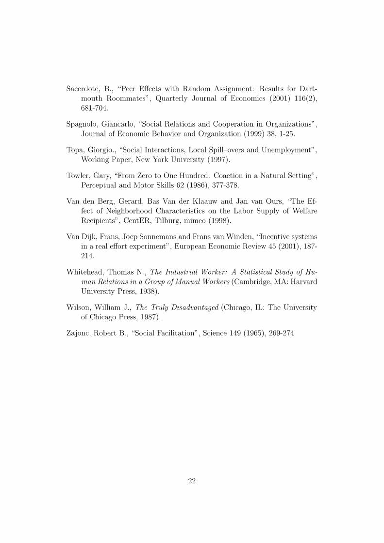
We chose a work task, which is simple, requires no previous knowledge

and is easy to measure. In particular, students had to prepare the mailing of

a questionnaire study for the University of Zurich. This job basically involved

stuffing letters into envelopes. First, subjects had to fold two sheets of paper

(one sheet contained the description of the questionnaire, the other was to

be filled out by the recipients of the study). After placing the two sheets

6

into the envelope, subjects had to seal the envelope and to put an A-priority

sticker on it. When a set of 25 envelopes had been completed the set had to

be bundled with a rubber band and put in a box. The work environment was

exactly the same for each subject, including, e.g., the same type of desk and

chair and the same large number of envelopes and sheets (Figure 1 displays

a picture of a subject’s desk). Payment was independent of output and paid

in cash. In both treatments the procedure was exactly the same.

2.3 Treatments

We study two treatments, the “pair” and the “single” treatment. In the pair

treatment two subjects did the task described above at the same time in the

same room. The two desks were situated in such a way that a subject could

easily realize the output of the other subject (the position of the second

desk can be seen in the background of Figure 1). Subjects were free to

communicate but instructed that they had to perform the task described

above independently. Hence, they were not allowed to engage in teamwork

or division of labor. We invited only students from different high-schools to

participate in this treatment in order to minimize the possibility that two

subjects in the pair treatment knew each other.

In the pair treatment peer effects were possible. In contrast, peer effects

were ruled out by design in the single treatment. In this control treatment

everything was exactly the same as in the pair treatment except that in

this case each subject worked alone in a room. Since subjects did not have

any contact to another subject and were not informed about other subjects’

output in this treatment, the single treatment rules out any potential peer

effect stemming from a co-worker. Therefore, a comparison of output arising

in the single treatment with that of the pair treatment, indicates the potential

7

effects of peers on productivity.

A total of 24 subjects participated in our study, eight in the single treat-

ment and 16 (eight pairs) in the pair treatment. The subjects were randomly

allocated to the treatments. No subject participated in more than one treat-

ment.

From a methodological point of view some aspects about the design are

worth pointing out: Unlike most lab experiments that study work behavior,

our subjects performed a ‘real’ task. In a typical lab experiment the choice

of work effort is represented by an increasing monetary function, i.e., instead

of choosing real effort subjects choose a costly number. This procedure has

been used in tournament experiments, e.g., Bull, Schotter and Weigelt [1987],

or in efficiency wage experiments, e.g., Fehr, Kirchsteiger and Riedl [1993].

Some authors have recently conducted so-called ‘real effort’ experiments to

study incentive mechanisms and efficiency wages. In Fahr and Irlenbusch

[2000] subjects had to crack walnuts, in van Dijk et al. [2001] subjects

performed cognitively demanding tasks on the computer (two-variable op-

timization problems) and in Gneezy [2003] subjects had to solve mazes at

the computer. However, the task is not perceived as economically valuable

at least in the latter two studies, meaning that an important dimension of

work which is usually performed is missing. In contrast, subjects performed

a regular and economically valuable job in our study.

3 Behavioral hypotheses

To illustrate in a simple way what we would expect to happen in the pair

treatment if peer effects existed, we assume that the output Xi of subject i

in a pair is given by

Xi = βXj + θi (1)

8

where Xj is the output of the other subject j, θi denotes the (random) innate

productivity of i and β measures how the output of i depends on the output

of j when they work in a pair. Within this context we say that peer effects

exist and are positive if the output of i increases with the output of j, which

formally means:

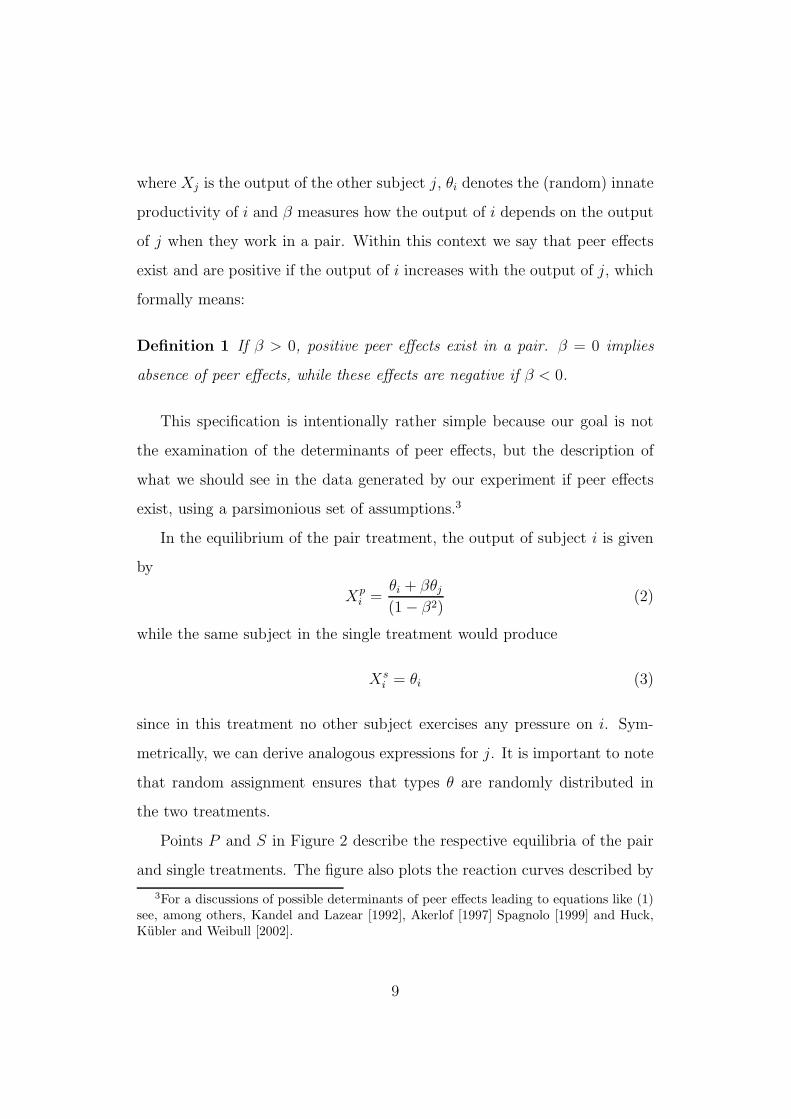
Definition 1 If β > 0, positive peer effects exist in a pair. β = 0 implies

absence of peer effects, while these effects are negative if β < 0.

This specification is intentionally rather simple because our goal is not

the examination of the determinants of peer effects, but the description of

what we should see in the data generated by our experiment if peer effects

exist, using a parsimonious set of assumptions.3

In the equilibrium of the pair treatment, the output of subject i is given

by

Xpi =

θi + βθj

(1 − β2)(2)

while the same subject in the single treatment would produce

Xsi = θi (3)

since in this treatment no other subject exercises any pressure on i. Sym-

metrically, we can derive analogous expressions for j. It is important to note

that random assignment ensures that types θ are randomly distributed in

the two treatments.

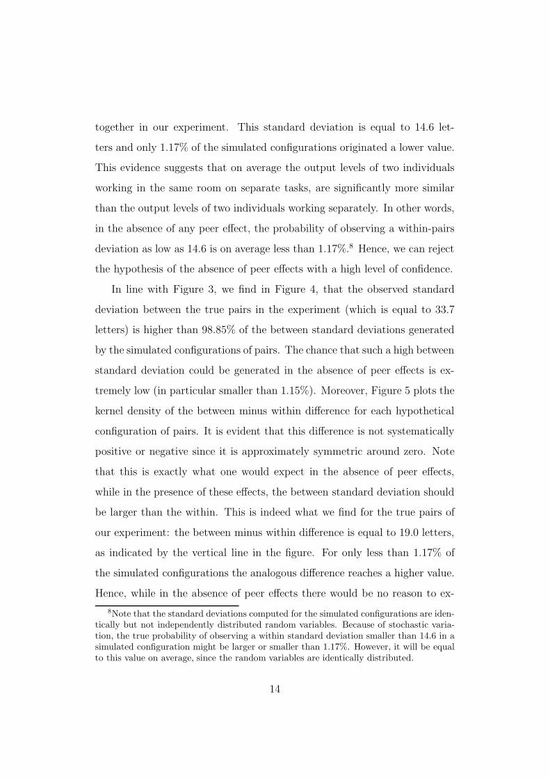
Points P and S in Figure 2 describe the respective equilibria of the pair

and single treatments. The figure also plots the reaction curves described by

3For a discussions of possible determinants of peer effects leading to equations like (1)see, among others, Kandel and Lazear [1992], Akerlof [1997] Spagnolo [1999] and Huck,Kubler and Weibull [2002].

9

equation (1) for the pair treatment, which cross at P , and by equation (3)

for the single treatment, which cross at S.

It is immediately obvious that the difference between the output levels of

the two subjects within each pair is equal to

∣∣∣XP

i − XPj

∣∣∣ =

|θi − θj |1 + β

. (4)

As a result, positive peer effects can be detected in the pair treatment ac-

cording to the following proposition, which will be tested in Section 4.

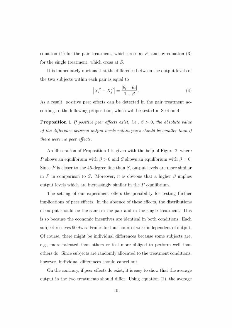
Proposition 1 If positive peer effects exist, i.e., β > 0, the absolute value

of the difference between output levels within pairs should be smaller than if

there were no peer effects.

An illustration of Proposition 1 is given with the help of Figure 2, where

P shows an equilibrium with β > 0 and S shows an equilibrium with β = 0.

Since P is closer to the 45-degree line than S, output levels are more similar

in P in comparison to S. Moreover, it is obvious that a higher β implies

output levels which are increasingly similar in the P equilibrium.

The setting of our experiment offers the possibility for testing further

implications of peer effects. In the absence of these effects, the distributions

of output should be the same in the pair and in the single treatment. This

is so because the economic incentives are identical in both conditions. Each

subject receives 90 Swiss Francs for four hours of work independent of output.

Of course, there might be individual differences because some subjects are,

e.g., more talented than others or feel more obliged to perform well than

others do. Since subjects are randomly allocated to the treatment conditions,

however, individual differences should cancel out.

On the contrary, if peer effects do exist, it is easy to show that the average

output in the two treatments should differ. Using equation (1), the average

10

output of i and j when they work in a pair is

XPi + XP

j

2=

θi+θj

2

1 − β(5)

while the average output of the same two subjects working alone in the single

treatment would beXS

i + XSj

2=

θi + θj

2(6)

A comparison of equations (5) and (6) shows that, in the presence of positive

peer effects such that 0 < β < 1, average output is higher in the pair treat-

ment than in the single treatment. This can also be inferred from Figure 2

where output in the P equilibrium is clearly higher compared to output in

the S equilibrium. If instead β > 1 the output level of the two subjects would

still be higher in the pair treatment but it would be equal to infinity. On

the contrary, in the case of negative effects (β < 0) the output of a subject

reduces the output of the other, in which case the output of the pair treat-

ment would be lower than the output of the single treatment. Our model

therefore suggests a second proposition, which will be tested in Section 4.

Proposition 2 In the presence of positive peer effects, the average output of

the pair treatment exceeds that of the single treatment.

Note that Proposition 2 states a behavioral consequence of peer effects,

which is similar to the so-called ‘social facilitation’ paradigm in social psy-

chology. According to this paradigm even the mere presence of another per-

son improves one’s performance. Numerous studies have supported evidence

for this type of behavior.4

4See for example Zajonc [1965], Cottrell et al. [1968] and Hunt and Hillery [1973]. InAllport [1920], performance of subjects doing simple tasks (like chain word association)was much better in groups than if subjects did the tasks alone. In a more recent study,Towler [1986] takes the time cars need to reach a 100-yards mark from a standing startat traffic lights. He reports that the if there are two cars at the traffic light the time totravel the 100 yards is significantly shorter than if there is just one car.

11

Our final proposition deals with the relationship between peer effects and

individual innate productivity. We have shown above that peer effects lead

to a higher output in the pair treatment compared to the single treatment.

We now ask how this increase depends on a subject’s innate productivity θ.

Assume that i is the more productive subject of a pair, i.e., θi > θj . This also

implies that i would produce more in the single treatment than j. Consider

further the difference ∆Xi = XPi − XS

i between the two potential output

levels for subject i in the pair and in the single treatment and, symmetrically

for j, consider also ∆Xj = XPj −XS

j . Using 2 and 3 it is easy to verify that

∆Xj > ∆Xi if 0 < β < 1 (7)

Equation (7) implies that if a finite equilibrium exists, the following propo-

sition holds (compare also XPi − XS

i and XPj − XS

j in Figure 2):

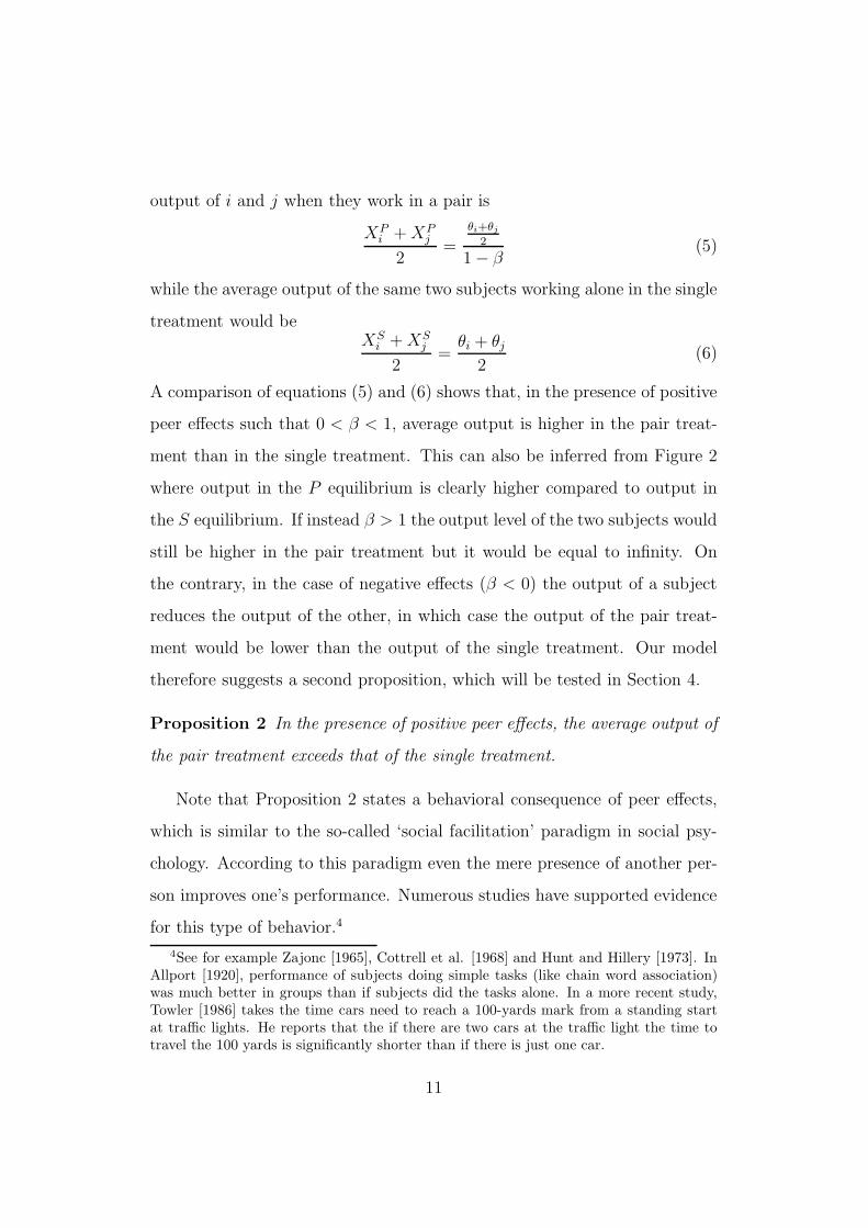
Proposition 3 Positive peer effects may lead to an individual output in-

crease, which is inversely related to the individual’s innate productivity θ.

Hence, our simple model suggests three propositions, which describe the

implications of peer effects in our treatments. We test these propositions in

the next section where we also show how our data can be used, in the light

of the model described above, to derive an implicit estimate of β.

4 Results

In this section we present our results and test our behavioral predictions.

Our main interest concerns the existence of positive peer effects, which are

revealed by the observation that output levels within pairs are similar in the

pair treatment. In order to test Proposition 1, consider the standard devi-

12

ation of output within and between pairs.5 In the absence of peer effects

(i.e., β = 0), working in a particular pair has no effect on individual behav-

ior. In this case, therefore, the standard deviations of output within pairs

should be identical to those generated by any simulated configuration of pairs

constructed from the same group of people. Moreover, there should be no

reason to expect that the between and within standard deviations obtained

with the true pairs should differ in any specific direction. Therefore, we can

construct a test for the endogenous formation of peer effects by comparing

the standard deviations generated by the true pairs of our experiment with

those generated by a random set of simulated configurations of pairs. This

comparison is shown in Figures 3, 4 and 5.

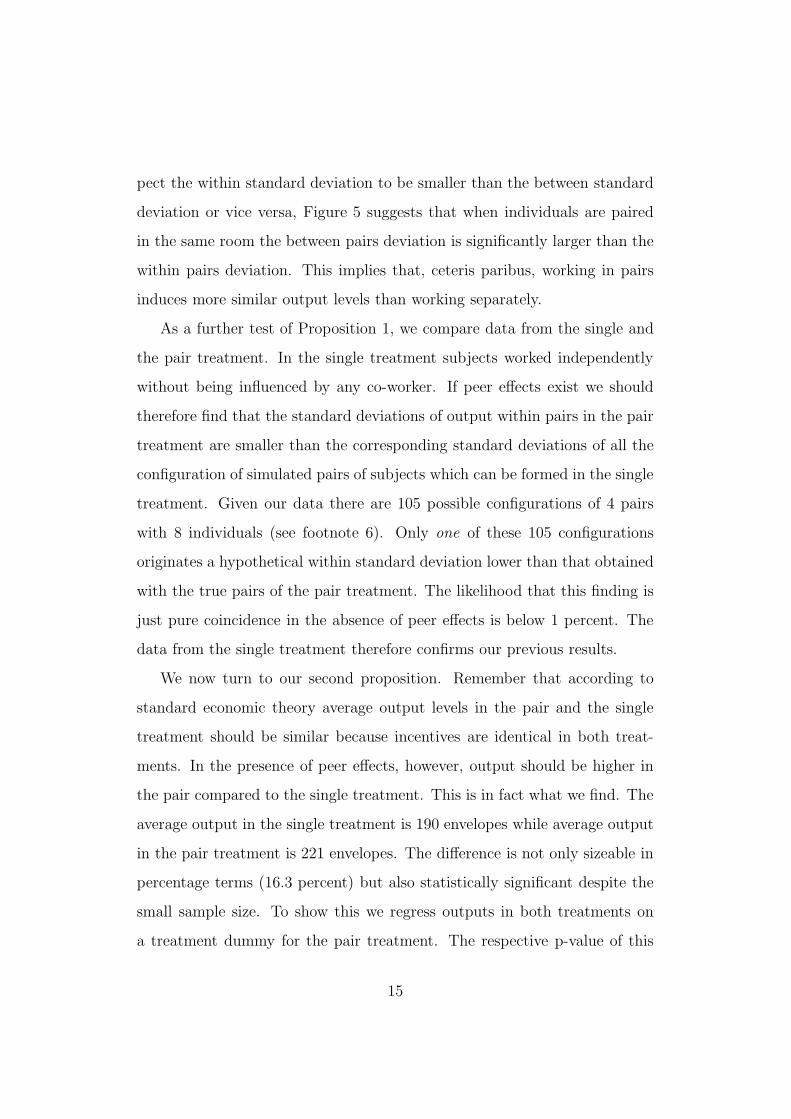
The first of these figures plots the kernel density of the simulated within

pairs standard deviations computed for 20,271 randomly chosen different

configurations of pairs of the 16 individuals involved in the pair treatment.

To be more precise, we generated all 2,027,025 possible configurations of

8 pairs with these 16 individuals6 and for one out of every 100 of these

configurations we computed the within pairs standard deviation.7

The variation of these simulated within standard deviations ranges from

9.6 to 34.8 letters. The vertical line in Figure 3 identifies the standard devia-

tion within true pairs, i.e., that computed for the pairs who actually worked

5We use standard deviations instead of differences to facilitate the computation and thecomparison of within and between statistics. This, however, does not change the substanceof our results because, in our specific case, the standard deviation within a pair is equalto the absolute value of the difference between the output levels of the pair divided by thesquare root of 2.

6 This number of configurations is in general equal to∏(N−2)/2

i=0 (N − 2i − 1), where Nis the (even) number of individuals, i.e. 16 in our case.

7We would have liked computing the within pairs standard deviations for all the2,027,025 configurations but this calculation would have required a substantial amountof computer time without any major gain from the viewpoint of the reliability of ourresults.

13

together in our experiment. This standard deviation is equal to 14.6 let-

ters and only 1.17% of the simulated configurations originated a lower value.

This evidence suggests that on average the output levels of two individuals

working in the same room on separate tasks, are significantly more similar

than the output levels of two individuals working separately. In other words,

in the absence of any peer effect, the probability of observing a within-pairs

deviation as low as 14.6 is on average less than 1.17%.8 Hence, we can reject

the hypothesis of the absence of peer effects with a high level of confidence.

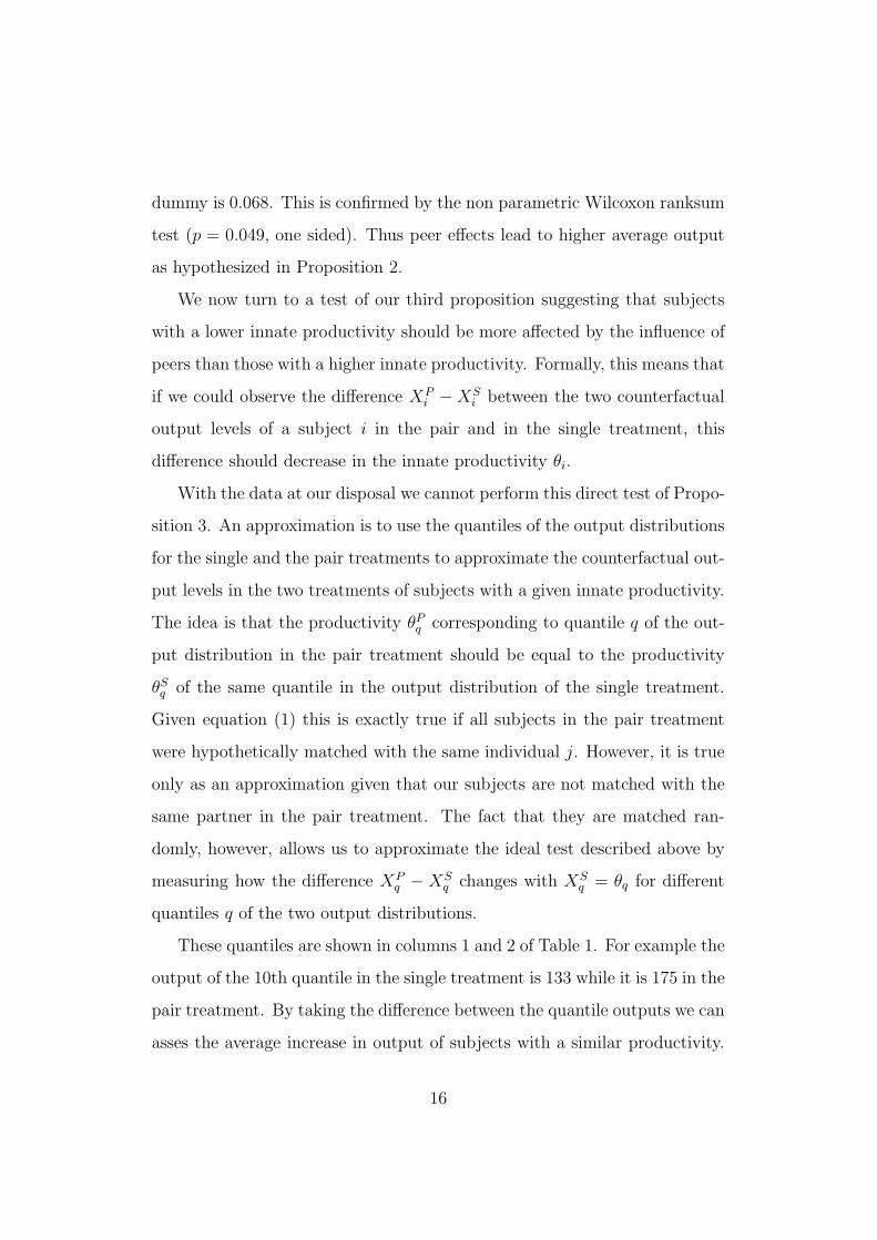
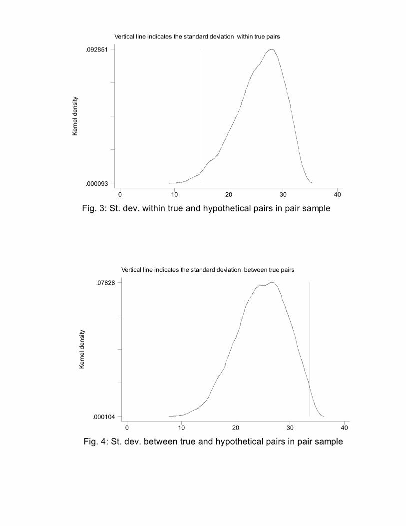
In line with Figure 3, we find in Figure 4, that the observed standard

deviation between the true pairs in the experiment (which is equal to 33.7

letters) is higher than 98.85% of the between standard deviations generated

by the simulated configurations of pairs. The chance that such a high between

standard deviation could be generated in the absence of peer effects is ex-

tremely low (in particular smaller than 1.15%). Moreover, Figure 5 plots the

kernel density of the between minus within difference for each hypothetical

configuration of pairs. It is evident that this difference is not systematically

positive or negative since it is approximately symmetric around zero. Note

that this is exactly what one would expect in the absence of peer effects,

while in the presence of these effects, the between standard deviation should

be larger than the within. This is indeed what we find for the true pairs of

our experiment: the between minus within difference is equal to 19.0 letters,

as indicated by the vertical line in the figure. For only less than 1.17% of

the simulated configurations the analogous difference reaches a higher value.

Hence, while in the absence of peer effects there would be no reason to ex-

8Note that the standard deviations computed for the simulated configurations are iden-tically but not independently distributed random variables. Because of stochastic varia-tion, the true probability of observing a within standard deviation smaller than 14.6 in asimulated configuration might be larger or smaller than 1.17%. However, it will be equalto this value on average, since the random variables are identically distributed.

14

pect the within standard deviation to be smaller than the between standard

deviation or vice versa, Figure 5 suggests that when individuals are paired

in the same room the between pairs deviation is significantly larger than the

within pairs deviation. This implies that, ceteris paribus, working in pairs

induces more similar output levels than working separately.

As a further test of Proposition 1, we compare data from the single and

the pair treatment. In the single treatment subjects worked independently

without being influenced by any co-worker. If peer effects exist we should

therefore find that the standard deviations of output within pairs in the pair

treatment are smaller than the corresponding standard deviations of all the

configuration of simulated pairs of subjects which can be formed in the single

treatment. Given our data there are 105 possible configurations of 4 pairs

with 8 individuals (see footnote 6). Only one of these 105 configurations

originates a hypothetical within standard deviation lower than that obtained

with the true pairs of the pair treatment. The likelihood that this finding is

just pure coincidence in the absence of peer effects is below 1 percent. The

data from the single treatment therefore confirms our previous results.

We now turn to our second proposition. Remember that according to

standard economic theory average output levels in the pair and the single

treatment should be similar because incentives are identical in both treat-

ments. In the presence of peer effects, however, output should be higher in

the pair compared to the single treatment. This is in fact what we find. The

average output in the single treatment is 190 envelopes while average output

in the pair treatment is 221 envelopes. The difference is not only sizeable in

percentage terms (16.3 percent) but also statistically significant despite the

small sample size. To show this we regress outputs in both treatments on

a treatment dummy for the pair treatment. The respective p-value of this

15

dummy is 0.068. This is confirmed by the non parametric Wilcoxon ranksum

test (p = 0.049, one sided). Thus peer effects lead to higher average output

as hypothesized in Proposition 2.

We now turn to a test of our third proposition suggesting that subjects

with a lower innate productivity should be more affected by the influence of

peers than those with a higher innate productivity. Formally, this means that

if we could observe the difference XPi − XS

i between the two counterfactual

output levels of a subject i in the pair and in the single treatment, this

difference should decrease in the innate productivity θi.

With the data at our disposal we cannot perform this direct test of Propo-

sition 3. An approximation is to use the quantiles of the output distributions

for the single and the pair treatments to approximate the counterfactual out-

put levels in the two treatments of subjects with a given innate productivity.

The idea is that the productivity θPq corresponding to quantile q of the out-

put distribution in the pair treatment should be equal to the productivity

θSq of the same quantile in the output distribution of the single treatment.

Given equation (1) this is exactly true if all subjects in the pair treatment

were hypothetically matched with the same individual j. However, it is true

only as an approximation given that our subjects are not matched with the

same partner in the pair treatment. The fact that they are matched ran-

domly, however, allows us to approximate the ideal test described above by

measuring how the difference XPq − XS

q changes with XSq = θq for different

quantiles q of the two output distributions.

These quantiles are shown in columns 1 and 2 of Table 1. For example the

output of the 10th quantile in the single treatment is 133 while it is 175 in the

pair treatment. By taking the difference between the quantile outputs we can

asses the average increase in output of subjects with a similar productivity.

16

If these differences decline as we move from the 10th to the 90th quantile,

we have evidence in favor of Proposition 3. Column 3 in Table 1 shows

that this difference in fact declines. The Spearman rank correlation between

these differences and the corresponding productivity levels is negative and

highly significant (Spearman’s rho = -0.900, p= 0.018 (one sided))9. Thus in

accordance with Proposition 3, the evidence suggests that low productivity

workers are more sensitive to the behavior of peers than are high productivity

workers.

We conclude this section by showing how, in the light of our simple model

of Section 3, the data generated by our experiment can be used to estimate β.

Remember that this parameter measures how the output of i influences the

output of j in a pair and vice versa. Equations (2) and (3) say that a subject

i’s outputs in the pair and the single treatments are given by Xpi =

θi+βθj

(1−β2)

and Xsi = θi, respectively. Substituting the sample averages Xp for Xp

i and

Xs for θi and θj , we can compute the average β solving Xp = Xs+βXs

(1−β2)or

221 = 190+β1901−β2 . This gives an implicit estimate of β = 0.14, which implies

that when the output of j increases by one unit, the output of i increases by

0.14 units on average. Of course, we do not claim that 0.14 is a universal

number. Yet, it is interesting and reassuring to see that Maggi and Ichino

(2000), who derive a comparable estimate of β with observational data, get

very similar numbers. Depending on the used controls and specifications

their estimates are β = 0.14, β = 0.18 and β = 0.15.

9In addition it is interesting to note that the bootstrapped p-values (of the test that thecorresponding quantiles are equal) increase in the quantile level. The p-values for the 10th,25th, 50th, 75th and 90th quantiles are 0.048, 0.145, 0.388, 0.432 and 0.788, respectively.These p-values are interesting for two reasons. First they show that only the differencefor the lowest quantile is significant. Second the probability that the respective quantilesfrom the single and the pair treatment are the same appears to increase monotonicallygoing from lower to higher quantiles of the output distribution.

17

5 Summary

In this paper we have presented clear and unambiguous evidence in favor of

the existence of peer effects. We show in a controlled field experiment that

the behavior of subjects working in pairs is significantly different than the

behavior of subjects working alone. The standard deviations within pairs

are significantly smaller than between pairs. As a second result, peer effects

work in the direction of raising the overall average productivity significantly.

We also show that the less productive workers react more significantly

to peer effects than do high productivity workers. In other words, “bad

apples”, far from damaging “good apples”, seem instead to gain in quality

when paired with these latter. This raises the interesting question of how

to allocate low and high productivity workers optimally. In the light of our

results, the output maximizing strategy might be to group low and high

productivity workers instead of grouping workers of similar productivity.

Note that in our study the presence of peer effects is robust and quan-

titatively important even though subjects interacted only once and did not

know each other. This suggests the possibility that the effects measured in

our study are a lower boundary for the effects that prevail in actual labor

relations.

In contrast with this conclusion, however, it can also be argued that a

setting of repeated interactions over a longer horizon might generate effects,

which cannot be easily predicted on the basis of our evidence. For example,

while in the short run the least productive workers seem to react to the

higher productivity of their peers, in the long run the opposite might be

true if it becomes clear that, as in our setting, low levels of output have no

consequences on rewards. To shed light on these issues, the next step in

18

our research agenda is to collect evidence on peer effects when interaction

between peers is repeated over longer horizons.

19

References

Aaronson, Daniel, “Using Sibling Data to Estimate the Impact of Neigh-

borhoods on Children’s Educational Outcomes”, Journal of Human Re-sources, XXIII (1998), 915–946.

Akerlof, George, “Social Distance and Social Decisions”, Econometrica 65(4),(1997), 1005-1027.

Allport, F.H., “The Influence of the Group upon Association and Thought”,Journal of Experimental Psychology 3 (1920), 159-182.

Bertrand, Marianne, Erzo F.P. Luttmer and Sendhil Mullainathan, “Net-work Effects and Welfare Cultures”, Quarterly Journal of Economics

115 (2000), 1019-1055.

Bull, C., Schotter, A. and K. Weigelt, “Tournaments and Piece Rates: An

Experimental Study”, Journal of Political Economy 95 (1987), 1-33.

Case, Anne, and Lawrence Katz, “The Company You Keep: The Effect ofFamily and Neighborhood on Disadvantaged Youth”, NBER Working

Paper 3705 (1991).

Cotrell, N. B., Wack, D. L., Sekerak, F. J. and R. H. Rittle, “Social Facili-

tation of Dominant Responses by the Presence of an Audience and theMere Presence of Others”, Journal of Personalitty and Social Psychology

10 (1968), 245-250.

Crane, Jonathan, “The Epidemic Theory of Ghettos and Neighborhood Ef-

fects on Dropping Out and Teenage Childbearing”, American Journalof Sociology XCVI (1991), 1226–1259.

Encinosa, William E., Martin Gaynor and James B. Rebitzer, “The Sociologyof Groups and the Economics of Incentives: Theory and Evidence on

Compensation Systems”, Case Western Reserve University (1998).

Fahr, Rene, and Bernd Irlenbusch, “Fairness as a Constraint on Trust inReciprocity: Earned Property Rights in a Reciprocal Exchange Experi-

ment”, Economics Letters 66 (2000), 275-282.

Falk A. and U. Fischbacher, “Crime in the Lab-detecting Social Interaction”,

European Economic Review 46 (2000), 859-869.

20

Falk, A., Fischbacher, U. and S. Gachter, “Isolating Social Interaction Effects- An Experimental Investigation”, IEW Working Paper 150, University

of Zurich (2003).

Fehr, E., Kirchsteiger, G. and A. Riedl, “Does Fairness Prevent Market Cear-

ing? An Experimental Investigation”, Quarterly Journal of Economics

108 (2) (1993), 437-459.

Glaeser, E. L., B. Sacerdote and Jose A. Scheinkman, “Crime and Social

Interactions”, Quarterly Journal of Economics CXI (1996), 507–548.

Gneezy, Uri, “Do High Wages Lead to High Profits? An Experimental Study

of Reciprocity Using Real Effort”, Working paper, University of Chicago,GSB 2003.

Huck, Steffen, Dorothea Kubler and Jorgen Weibull, “Social Norms and In-centives in Firms”, mimeo, University College London (2002).

Hunt, Peter J., and Joseph M. Hillery, “Social Facilitation in a CoactionSetting: An Examination of the Effects Over Learning Trials”, Journal

of Experimental Social Psychology 9 (1973), 563-571.

Ichino A. and G. Maggi, “Work Environment and Individual Background:Explaining Regional Shirking Differentials in a Large Italian Firm” Quar-

terly Journal of Economics 115 (2000), 1057-1090.

Jones, R. G. Stephen, “Worker Interdependence and Output: The Hawthorne

Studies Reevaluated”, American Sociological Review LV (1990), 176–190.

Kandel, E. and E. P. Lazear, “Peer Pressure and Partnerships”, Journal of

Political Economy 100 (4) (1992), 801-817.

Katz L., J. R. Kling and J. B. Liebman, “ Moving to Opportunities in Boston:

Early results of a Randomized Mobility Experiment”, Quarterly Journalof Economics 116(2) (2001) , 607-654.

Manski, Charles F., “Identification of Endogenous Social Effects: The Re-flection Problem”, Review of Economic Studies LX (1993), 531–542.

Nagin, D. S., Rebitzer J. B., Sanders S. and J. L. Taylor, “Monitoring, Moti-

vation and Management: The Determinants of Opportunistic Behaviorin a Field Experiment”, American Economic Review, 92 (4) (2002), 850-

873.

21

Sacerdote, B., “Peer Effects with Random Assignment: Results for Dart-mouth Roommates”, Quarterly Journal of Economics (2001) 116(2),

681-704.

Spagnolo, Giancarlo, “Social Relations and Cooperation in Organizations”,

Journal of Economic Behavior and Organization (1999) 38, 1-25.

Topa, Giorgio., “Social Interactions, Local Spill–overs and Unemployment”,Working Paper, New York University (1997).

Towler, Gary, “From Zero to One Hundred: Coaction in a Natural Setting”,Perceptual and Motor Skills 62 (1986), 377-378.

Van den Berg, Gerard, Bas Van der Klaauw and Jan van Ours, “The Ef-fect of Neighborhood Characteristics on the Labor Supply of Welfare

Recipients”, CentER, Tilburg, mimeo (1998).

Van Dijk, Frans, Joep Sonnemans and Frans van Winden, “Incentive systems

in a real effort experiment”, European Economic Review 45 (2001), 187-214.

Whitehead, Thomas N., The Industrial Worker: A Statistical Study of Hu-

man Relations in a Group of Manual Workers (Cambridge, MA: HarvardUniversity Press, 1938).

Wilson, William J., The Truly Disadvantaged (Chicago, IL: The Universityof Chicago Press, 1987).

Zajonc, Robert B., “Social Facilitation”, Science 149 (1965), 269-274

22

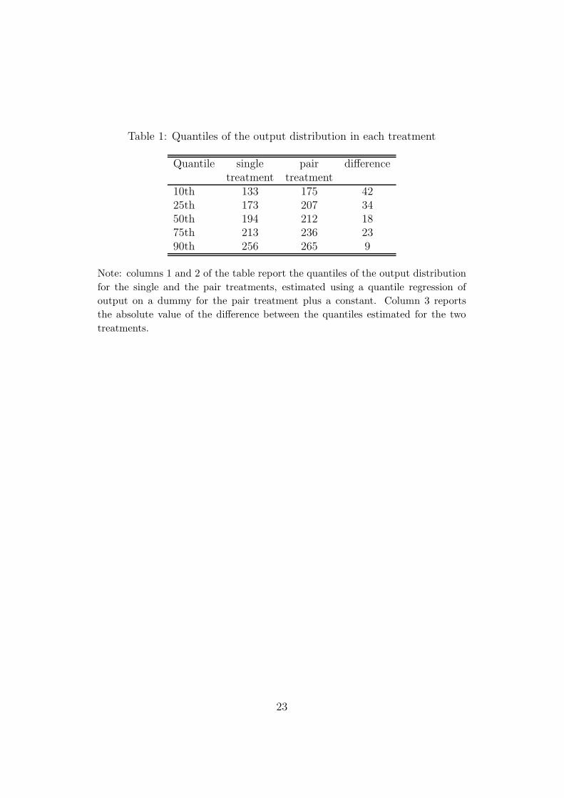
Table 1: Quantiles of the output distribution in each treatment

Quantile single pair differencetreatment treatment

10th 133 175 4225th 173 207 3450th 194 212 1875th 213 236 2390th 256 265 9

Note: columns 1 and 2 of the table report the quantiles of the output distributionfor the single and the pair treatments, estimated using a quantile regression ofoutput on a dummy for the pair treatment plus a constant. Column 3 reportsthe absolute value of the difference between the quantiles estimated for the twotreatments.

23

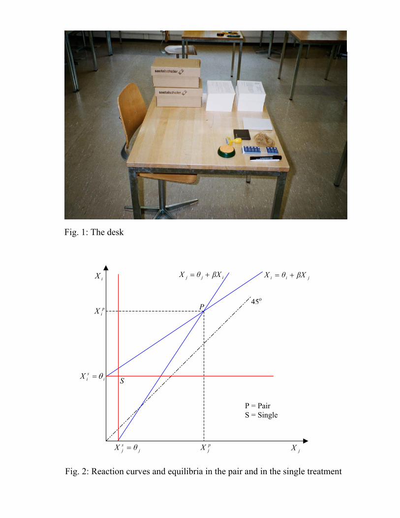
Fig. 1: The desk

Fig. 2: Reaction curves and equilibria in the pair and in the single treatment

P

S

P = PairS = Single

45o

pjX jXj

sj θX =

isiX θ=

piX

iX ijj βXθX += jii βXθX +=

Vertical line indicates the standard deviation within true pairs

Ke

rnel

den

sity

Fig. 3: St. dev. within true and hypothetical pairs in pair sample

0 10 20 30 40

.000093

.092851

Vertical line indicates the standard deviation between true pairs

Ke

rnel

den

sity

Fig. 4: St. dev. between true and hypothetical pairs in pair sample

0 10 20 30 40

.000104

.07828

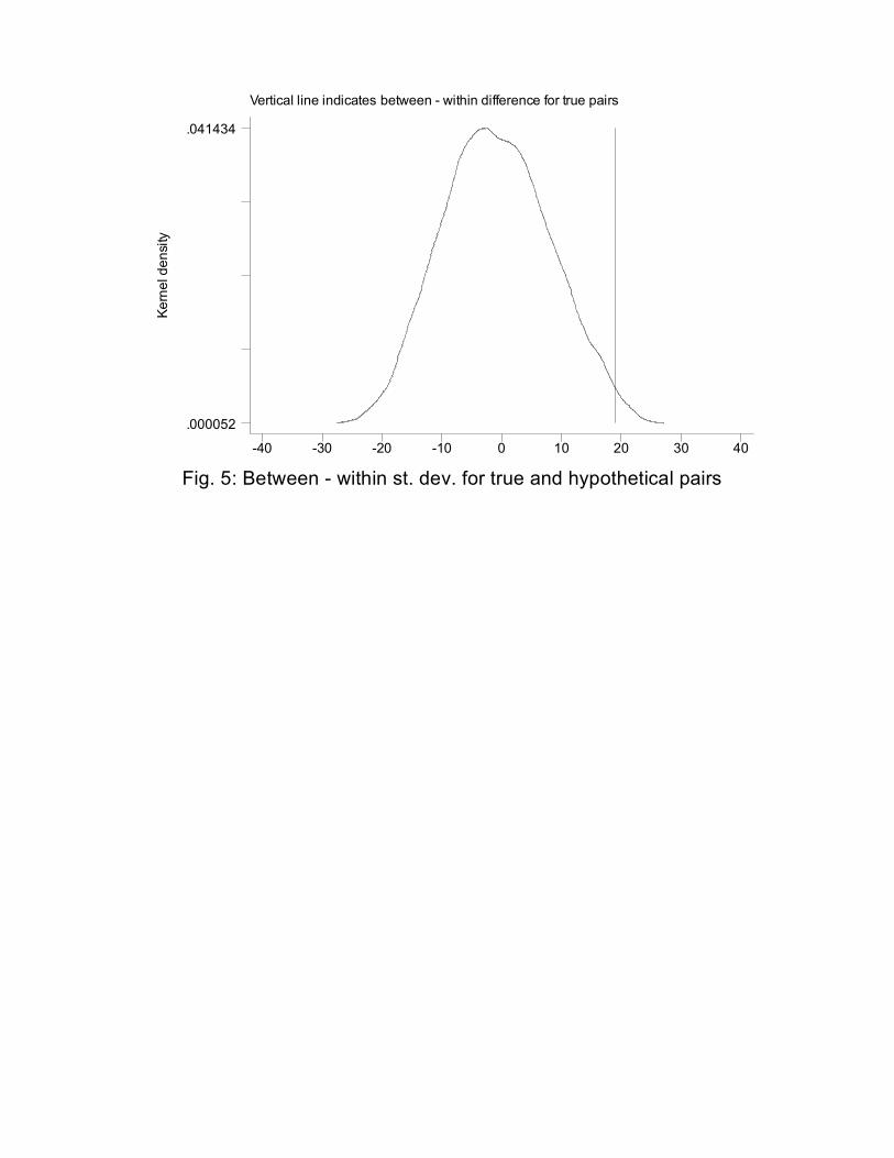
Vertical line indicates between - within difference for true pairs

Ke

rnel

den

sity

Fig. 5: Between - within st. dev. for true and hypothetical pairs

-40 -30 -20 -10 0 10 20 30 40

.000052

.041434

IZA Discussion Papers No.

Author(s) Title

Area Date

716 M. Rosholm L. Skipper

Is Labour Market Training a Curse for the Unemployed? Evidence from a Social Experiment

6 02/03

717 A. Hijzen H. Görg R. C. Hine

International Fragmentation and Relative Wages in the UK

2 02/03

718 E. Schlicht

Consistency in Organization 1 02/03

719 J. Albrecht P. Gautier S. Vroman

Equilibrium Directed Search with Multiple Applications

3 02/03

720 T. Palokangas Labour Market Regulation, Productivity-Improving R&D and Endogenous Growth

3 02/03

721 H. Battu M. Mwale Y. Zenou

Do Oppositional Identities Reduce Employment for Ethnic Minorities?

1 02/03

722 C. K. Spiess F. Büchel G. G. Wagner

Children's School Placement in Germany: Does Kindergarten Attendance Matter?

6 02/03

723 M. Coles B. Petrongolo

A Test between Unemployment Theories Using Matching Data

3 02/03

724 J. T. Addison R. Bailey W. S. Siebert

The Impact of Deunionisation on Earnings Dispersion Revisited

2 02/03

725 S. Habermalz An Examination of Sheepskin Effects Over Time 1 02/03

726 S. Habermalz Job Matching and the Returns to Educational Signals

1 02/03

727 M. Raiser M. Schaffer J. Schuchardt

Benchmarking Structural Change in Transition 4 02/03

728 M. Lechner J. A. Smith

What is the Value Added by Caseworkers? 6 02/03

729 A. Voicu H. Buddelmeyer

Children and Women's Participation Dynamics: Transitory and Long-Term Effects

3 02/03

730 M. Piva M. Vivarelli

Innovation and Employment: Evidence from Italian Microdata

2 02/03

731 B. R. Chiswick N. DebBurman

Educational Attainment: Analysis by Immigrant Generation

1 02/03

732 A. Falk A. Ichino

Clean Evidence on Peer Pressure 5 03/03

An updated list of IZA Discussion Papers is available on the center‘s homepage www.iza.org.