Embed Size (px)
Citation preview

Clawpack TutorialPart 2
Randall J. LeVequeApplied Mathematics
University of Washington
Slides posted atwww.clawpack.org/links/tutorials
Randy LeVeque Clawpack Tutorial at the IMA, October 2010
Outline
• Makefiles• Specifying run-time parameters• Specifying boundary conditions• Riemann solvers
Randy LeVeque Clawpack Tutorial at the IMA, October 2010

Application Makefile
Documentation: www.clawpack.org/doc/makefiles.htmlFor example, see $CLAW/apps/acoustics/1d/example2/Makefile
Several variables are set, e.g.where to find setrun function and where to put output:
CLAW_setrun_file = setrun.pyCLAW_OUTDIR = _output
where to find setplot function and where to put plots:
CLAW_setplot_file = setplot.pyCLAW_PLOTDIR = _plots
Usually these do not need to be changed.
Randy LeVeque Clawpack Tutorial at the IMA, October 2010

Application Makefile (cont.)
List of local Fortran files:
CLAW_SOURCES = \driver.f \qinit.f \rp1.f \setprob.f
List of library files:
# Clawpack library to be used:CLAW_LIB = $(CLAW)/clawpack/1d/lib
CLAW_LIBSOURCES = \$(CLAW_LIB)/claw1ez.f \$(CLAW_LIB)/bc1.f \etc.
Randy LeVeque Clawpack Tutorial at the IMA, October 2010

Application Makefile (cont.)
Ends with...
# Include Makefile containing standard# definitions and make options:CLAWMAKE = $(CLAW)/util/Makefile.commoninclude $(CLAWMAKE)
The file $CLAW/util/Makefile.common contains rules for varioustargets.
For possible targets, type
$ make help
Documentation: www.clawpack.org/doc/makefiles.html
Randy LeVeque Clawpack Tutorial at the IMA, October 2010

Setting runtime parameters
The file setrun.py contains a function setrunthat returns an object rundata of class ClawRunData.
Never need to write from scratch...Modify an existing example!
Don’t need to know much if anything about Python!
Lots of comments in the sample versions.
Documentation: www.clawpack.org/doc/setrun.html
For example, see $CLAW/apps/acoustics/1d/example2/setrun.py
Randy LeVeque Clawpack Tutorial at the IMA, October 2010
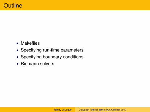
Copying and modifying an example
Find an example similar to the one you want to create and copythe directory, e.g.
$ cd $CLAW/apps/acoustics/1d$ cp -r example2 $CLAW/myclaw/newexample
Warning: If you have a Subversion copy of Clawpack...This will copy .svn subdirectory too.Better way:
$ cd $CLAW/apps/acoustics/1d$ svn export example2 $CLAW/myclaw/newexample
Documentation: www.clawpack.org/doc/newapp.html
Randy LeVeque Clawpack Tutorial at the IMA, October 2010

The Riemann problem
The Riemann problem consists of the hyperbolic equationunder study together with initial data of the form
q(x, 0) ={ql if x < 0qr if x ≥ 0
Piecewise constant with a single jump discontinuity from ql toqr.
The Riemann problem is fundamental to understanding• The mathematical theory of hyperbolic problems,• Godunov-type finite volume methods
Why? Even for nonlinear systems of conservation laws, theRiemann problem can often be solved for general ql and qr, andconsists of a set of waves propagating at constant speeds.
Randy LeVeque Clawpack Tutorial at the IMA, October 2010

Linear hyperbolic systems
Linear system of m equations: q(x, t) ∈ lRm for each (x, t) and
qt +Aqx = 0, −∞ < x,∞, t ≥ 0.
A is m×m with eigenvalues λp and eigenvectors rp,for p = 1, 2, , . . . , m:
Arp = λprp.
Combining these for p = 1, 2, , . . . , m gives
AR = RΛ
where
R = [r1 r2 · · · rm], Λ = diag(λ1, λ2, . . . , λm).
The system is hyperbolic if the eigenvalues are real andR is invertible. Then A can be diagonalized:
R−1AR = Λ
Randy LeVeque Clawpack Tutorial at the IMA, October 2010

Linear hyperbolic systems
Let R be matrix of right eigenvectors and v(x, t) = R−1q(x, t).Multiply system qt +Aqx = 0 by R−1 on left to obtain
R−1qt +R−1ARR−1qx = 0
Since R−1AR = Λ, this diagonalizes the system:
wt + Λwx = 0.
This is a system of m decoupled advection equations
wpt + λpwp
x = 0.
Sowp(x, t) = wp(x− λpt, 0)
where w(x, 0) = R−1q(x, 0) = R−1η(x).
Randy LeVeque Clawpack Tutorial at the IMA, October 2010

Linear acoustics
Example: Linear acoustics in a 1d gas tube
q =[pu
]p(x, t) = pressure perturbationu(x, t) = velocity
Equations:
pt + κux = 0 Change in pressure due to compressionρut + px = 0 Newton’s second law, F = ma
where K = bulk modulus, and ρ = unperturbed density of gas.
Hyperbolic system:[pu
]t
+[
0 κ1/ρ 0
] [pu
]x
= 0.
Randy LeVeque Clawpack Tutorial at the IMA, October 2010

Linear acoustics
[pu
]t
+[
0 κ1/ρ 0
] [pu
]x
= 0.
This has the form qt +Aqx = 0 with
eigenvalues: λ1 = −c, λ2 = +c,
where c =√κ/ρ = speed of sound.
eigenvectors: r1 =[−Z1
], r2 =
[Z1
]where Z = ρc =
√ρκ = impedance.
R =[−Z Z1 1
], R−1 =
12Z
[−1 Z1 Z
].
Randy LeVeque Clawpack Tutorial at the IMA, October 2010

Riemann Problem
Special initial data:
q(x, 0) ={ql if x < 0qr if x > 0
Example: Acoustics with bursting diaphram (ul = ur = 0)
Pressure:
Acoustic waves propagate with speeds ±c.Randy LeVeque Clawpack Tutorial at the IMA, October 2010

Riemann Problem
Special initial data:
q(x, 0) ={ql if x < 0qr if x > 0
Example: Acoustics with bursting diaphram (ul = ur = 0)
Pressure:
Acoustic waves propagate with speeds ±c.Randy LeVeque Clawpack Tutorial at the IMA, October 2010

Riemann Problem
Special initial data:
q(x, 0) ={ql if x < 0qr if x > 0
Example: Acoustics with bursting diaphram (ul = ur = 0)
Pressure:
Acoustic waves propagate with speeds ±c.Randy LeVeque Clawpack Tutorial at the IMA, October 2010

Riemann Problem
Special initial data:
q(x, 0) ={ql if x < 0qr if x > 0
Example: Acoustics with bursting diaphram (ul = ur = 0)
Pressure:
Acoustic waves propagate with speeds ±c.Randy LeVeque Clawpack Tutorial at the IMA, October 2010

Riemann Problem for acoustics
ql = w1l r
1 + w2l r
2
qr = w1rr
1 + w2rr
2
Thenqm = w1
rr1 + w2
l r2
So the wavesW1 andW2 are eigenvectors of A:
W1 = qm − ql = (w1r − w1
l )r1
W2 = qr − qm = (w2r − w2
l )r2.
Randy LeVeque Clawpack Tutorial at the IMA, October 2010

Riemann Problem for acoustics
Waves propagating in x–t space:
Left-going waveW1 = qm − ql andright-going waveW2 = qr − qm are eigenvectors of A.
Randy LeVeque Clawpack Tutorial at the IMA, October 2010

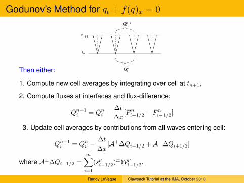
Godunov’s Method for qt + f(q)x = 0
Then either:
1. Compute new cell averages by integrating over cell at tn+1,
2. Compute fluxes at interfaces and flux-difference:
Qn+1i = Qni −
∆t∆x
[Fni+1/2 − Fni−1/2]
3. Update cell averages by contributions from all waves entering cell:
Qn+1i = Qni −
∆t∆x
[A+∆Qi−1/2 +A−∆Qi+1/2]
where A±∆Qi−1/2 =m∑i=1
(spi−1/2)±Wpi−1/2.
Randy LeVeque Clawpack Tutorial at the IMA, October 2010

Wave-propagation viewpoint
For linear system qt +Aqx = 0, the Riemann solution consists of
wavesWp propagating at constant speed λp.λ2∆t
W1i−1/2
W1i+1/2
W2i−1/2
W3i−1/2
Qi −Qi−1 =m∑
p=1
αpi−1/2r
p ≡m∑
p=1
Wpi−1/2.
Qn+1i = Qn
i −∆t∆x[λ2W2
i−1/2 + λ3W3i−1/2 + λ1W1
i+1/2
].
Randy LeVeque Clawpack Tutorial at the IMA, October 2010

CLAWPACK Riemann solver
The hyperbolic problem is specified by the Riemann solver• Input: Values of q in each grid cell
• Output: Solution to Riemann problem at each interface.• WavesWp ∈ lRm, p = 1, 2, . . . , Mw
• Speeds sp ∈ lR, p = 1, 2, . . . , Mw,
• Fluctuations A−∆Q, A+∆Q ∈ lRm
Note: Number of waves Mw often equal to m (length of q),but could be different (e.g. HLL solver has 2 waves).
Fluctuations:
A−∆Q = Contribution to cell average to left,A+∆Q = Contribution to cell average to right
For conservation law, A−∆Q+A+∆Q = f(Qr)− f(Ql)
Randy LeVeque Clawpack Tutorial at the IMA, October 2010

CLAWPACK Riemann solver
Inputs to rp1 subroutine:
ql(i,1:m) = Value of q at left edge of ith cell,
qr(i,1:m) = Value of q at right edge of ith cell,
Warning: The Riemann problem at the interface between cellsi− 1 and i has left state qr(i-1,:) and right state ql(i,:).
rp1 is normally called with ql = qr = q,but designed to allow other methods:
Randy LeVeque Clawpack Tutorial at the IMA, October 2010

CLAWPACK Riemann solver
Outputs from rp1 subroutine:
for system of m equationswith mw ranging from 1 to Mw =# of waves
s(i,mw) = Speed of wave # mw in ith Riemann solution,
wave(i,1:m,mw) = Jump across wave # mw,
amdq(i,1:m) = Left-going fluctuation, updates Qi−1
apdq(i,1:m) = Right-going fluctuation, updates Qi
Randy LeVeque Clawpack Tutorial at the IMA, October 2010

Boundary conditions and ghost cells
In each time step, the data in cells 1 to N = mx is used todefine ghost cell values in cells outside the physical domain.
The wave-propagation algorithm is then applied on theexpanded computational domain, solving Riemann problems atall interfaces.
The data is extended depending on the physical boundaryconditons.
Randy LeVeque Clawpack Tutorial at the IMA, October 2010

Boundary conditions
....Q−1 Q0 Q1 Q2 QN QN+1 QN+2
x1/2
x = a
xN+1/2
x = b
Periodic:
Qn−1 = Qn
N−1, Qn0 = Qn
N , QnN+1 = Qn
1 , QnN+2 = Qn
2
Extrapolation (outflow):
Qn−1 = Qn
1 , Qn0 = Qn
1 , QnN+1 = Qn
N , QnN+2 = Qn
N
Solid wall:For Q0 : p0 = p1, u0 = −u1,
For Q−1 : p−1 = p2, u−1 = −u2.
Randy LeVeque Clawpack Tutorial at the IMA, October 2010

Setting BCs in Clawpack
In setrun.py, at each boundary(xlower, xupper, ylower, yupper)
must specify for example:
clawdata.mthbc_xlower = 3 # solid wallclawdata.mthbc_xupper = 1 # extrapolation
Set to 2 at both boundaries for periodic.
Set to 0 if you want to impose something special.
In this case need to copy $CLAW/clawpack/1d/lib/bc1.f toapplication directory and modify (along with Makefile).
Randy LeVeque Clawpack Tutorial at the IMA, October 2010

Extrapolation boundary conditions
If we set Q0 = Q1 then the Riemann problem at x1/2 has zerostrength waves:
Q1 −Q0 =W11/2 +W2
1/2
So in particular the incoming waveW2 has strength 0.
The outgoing wave perhaps should have nonzero magnitude,but it doesn’t matter since it would only update ghost cell.
Ghost cell value is reset at the start of each time step byextrapolation.
In 2D or 3D, extrapolation in normal direction is not perfect butworks quite well.
Randy LeVeque Clawpack Tutorial at the IMA, October 2010

Extrapolation boundary conditions
Examples:
• One-dimensional acoustics:$CLAW/book/chap3/acousimple$CLAW/apps/acoustics/1d/example2
• Tsunami propagation:$CLAW/apps/tsunami/chile2010
• Seismic waves in a half-space on following slides,
Randy LeVeque Clawpack Tutorial at the IMA, October 2010

Equations of linear elasticity (in 2d)
σ11t − (λ+ 2µ)ux − λvy = 0
σ22t − λux − (λ+ 2µ)vy = 0
σ12t − µ(vx + uy) = 0
ρut − σ11x − σ12
y = 0
ρvt − σ12x − σ22
y = 0
where λ(x, y) and µ(x, y) are Lamé parameters.
This has the form qt +Aqx +Bqy = 0.
The matrix (A cos θ +B sin θ) has eigenvalues −cp, −cs, 0, cs, cp
P-wave (dilatational) speed: cp =√
λ+2µρ
S-wave (shear) speed: cs =√
µρ
Randy LeVeque Clawpack Tutorial at the IMA, October 2010

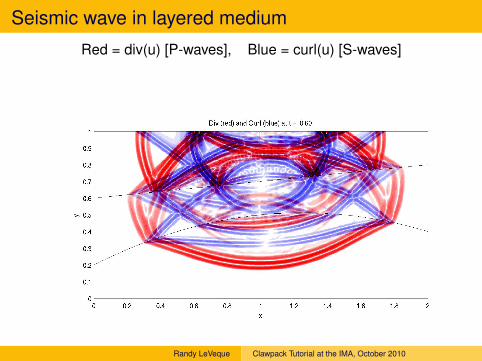
Seismic waves in layered earth
Layers 1 and 3: ρ = 2, λ = 1, µ = 1, cp ≈ 1.2, cs ≈ 0.7
Layer 2: ρ = 5, λ = 10, µ = 5, cp = 2.0, cs = 1
Impulse at top surface at t = 0.
Solved on uniform Cartesian grid (600× 300).
Cell average of material parameters used in each finite volumecell.
Extrapolation at computational boundaries.
Randy LeVeque Clawpack Tutorial at the IMA, October 2010

Seismic wave in layered medium
Red = div(u) [P-waves], Blue = curl(u) [S-waves]
Randy LeVeque Clawpack Tutorial at the IMA, October 2010

Seismic wave in layered medium
Red = div(u) [P-waves], Blue = curl(u) [S-waves]
Randy LeVeque Clawpack Tutorial at the IMA, October 2010

Seismic wave in layered medium
Red = div(u) [P-waves], Blue = curl(u) [S-waves]
Randy LeVeque Clawpack Tutorial at the IMA, October 2010

Seismic wave in layered medium
Red = div(u) [P-waves], Blue = curl(u) [S-waves]
Randy LeVeque Clawpack Tutorial at the IMA, October 2010

Seismic wave in layered medium
Red = div(u) [P-waves], Blue = curl(u) [S-waves]
Randy LeVeque Clawpack Tutorial at the IMA, October 2010
Seismic wave in layered medium
Red = div(u) [P-waves], Blue = curl(u) [S-waves]
Randy LeVeque Clawpack Tutorial at the IMA, October 2010

Seismic wave in layered medium
Red = div(u) [P-waves], Blue = curl(u) [S-waves]
Randy LeVeque Clawpack Tutorial at the IMA, October 2010

Seismic wave in layered medium
Red = div(u) [P-waves], Blue = curl(u) [S-waves]
Randy LeVeque Clawpack Tutorial at the IMA, October 2010

Seismic wave in layered medium
Red = div(u) [P-waves], Blue = curl(u) [S-waves]
Randy LeVeque Clawpack Tutorial at the IMA, October 2010

Seismic wave in layered medium
Red = div(u) [P-waves], Blue = curl(u) [S-waves]
Randy LeVeque Clawpack Tutorial at the IMA, October 2010