Embed Size (px)
Citation preview
TSE-0061-0306 1
Abstract— This paper introduces a new technique for finding latent software bugs called change classification. Change
classification uses a machine learning classifier to determine whether a new software change is more similar to prior
buggy changes, or clean changes. In this manner, change classification predicts the existence of bugs in software changes.
The classifier is trained using features (in the machine learning sense) extracted from the revision history of a software
project, as stored in its software configuration management repository. The trained classifier can classify changes as
buggy or clean with 78% accuracy and 65% buggy change recall (on average). Change classification has several desirable
qualities: (1) the prediction granularity is small (a change to a single file), (2) predictions do not require semantic
information about the source code, (3) the technique works for a broad array of project types and programming
languages, and (4) predictions can be made immediately upon completion of a change. Contributions of the paper include
a description of the change classification approach, techniques for extracting features from source code and change
histories, a characterization of the performance of change classification across 12 open source projects, and evaluation of
the predictive power of different groups of features.
Index Terms-- Maintenance, Software metrics, Software fault diagnosis, Configuration management, Classification,
Association rules, Data mining.
I. INTRODUCTION
Consider a software developer working on a long duration software product. Like most
software developers, she typically makes changes that are clean, not containing a latent bug. At
times she makes changes that introduce new features, or adapts the software to a changing
operational environment. Sometimes she makes bug-fix changes that repair a bug. Occasionally
she makes a bug-introducing change and injects incorrect statements into the source code. Since
developers typically do not know they are writing incorrect software, there is always the question
of whether the change they just made has introduced a bug.
A bug in the source code leads to an unintended state within the executing software, and this
corrupted state eventually results in an undesired external behavior. This is logged in a bug
report message in a change tracking system, often many months after the initial injection of the
bug into the software. By the time a developer receives the bug report, she must spend time to
Manuscript received March 10, 2006. This work is supported by NSF Grant CCR-01234603, and a Cooperative Agreement with NASA Ames
Research Center.
S. Kim is with Massachusetts Institute of Technology, Cambridge, MA USA (telephone: 617-253-1947, e-mail: [email protected]).
E. J. Whitehead, Jr. is with University of California, Santa Cruz, CA 95064 USA (telephone: 831-459-1227, e-mail: [email protected]).
Y. Zhang is with University of California, Santa Cruz, CA 95064 USA (telephone: 831-459-4549, e-mail: [email protected]).
Classifying Software Changes: Clean or Buggy?
Sunghun KIM, E. James WHITEHEAD, Jr., Member, IEEE, and Yi ZHANG, Member, IEEE

TSE-0061-0306 2
reacquaint themselves with the source code and the recent changes made to it. This is time
consuming.
If there were a tool that could accurately predict whether a change was buggy or clean
immediately after a change was made, it would permit developers to take steps to fix the
introduced bugs immediately. Several bug finding techniques could be used, including code
inspections, unit testing, and use of static analysis tools. Since these steps would be taken right
after a code change was made, the developer would still retain the full mental context of the
change. This holds promise for reducing the time required to find software bugs, as well as
reducing the time that bugs stay resident in software before removal.
This paper presents a new technique, called change classification, for predicting bugs in file-
level software changes (a set of line ranges in a single file changed since the previous revision)
using machine learning classification algorithms. A key insight behind this work is viewing bug
prediction in changes as a kind of classification problem, that is, assigning each change made
into one of two classes: clean changes or buggy changes.
The change classification technique involves two steps: training and classification. The change
classification algorithms learn from a training set, i.e., a collection of changes that are known to
belong to an existing class, that is, the changes are labeled with the known class. Features are
extracted from the changes, and the classification algorithm learns which features are most useful
for discriminating among the various classes. In this context, feature often means some property
of the change, such as the frequency of words that are present in source code. This is different
from the typical software engineering notion of feature as a software functionality.
Unfortunately for software change classification, we do not have a known standard corpus like
the UCI Repository of machine learning [37] or the Reuters Corpus [23] which is commonly

TSE-0061-0306 3
used for evaluation in the text classification domain. Instead, in this paper the file change
histories of 12 open source projects are extracted from their software configuration management
systems (SCMs), and then features are mined from each change, creating the corpus used to
evaluate change classification per project. Each project’s features are used to train an Support
Vector Machine (SVM) [14] classifier for that project. SVMs are a class of high performance
machine learning classification algorithms that have good behavior for a range of text
classification problems. After training an SVM using change data from revision 1 to n, if there is
a new and unclassified change (i.e., revision n+1), this change can be classified as either buggy
or clean using the trained classifier model. This act of classification has the effect of predicting
which changes have bugs.
This paper makes the following contributions:
New bug prediction technique: change classification. Use of machine learning classifiers, as
trained on software evolution data and applied to software changes (instead of entire files,
functions, or methods), provide a new method for predicting the location of latent software bugs.
Evaluation of the performance of change classification. The classification accuracy, recall, and
precision are evaluated for each project. An SVM classifies file changes as buggy or clean with
78% accuracy on average (ranging by project from 64%-93% as shown in Figure 2) and 65%
buggy change recall on average (43%-98% as shown in Figure 2). This is on par with the best
recent work on bug prediction in the research literature [12] [39], with the added benefit that the
granularity of prediction is smaller: it is localized to the section of text related to a change
instead of a whole file or function/method.
Techniques for feature extraction from source code and change histories. In order to extract
features from a software evolution history, new techniques for feature extraction were developed.

TSE-0061-0306 4
These have utility for any researcher performing classification experiments using evolution data.
Evaluation of the performance of individual features, and groups of features. Since the choice
of features can affect the performance of classifiers, each feature’s discriminative power for
performing change classification is compared. This is performed by evaluating which set of
features yields the best overall classification accuracy and recall, and also by examining the
relative contributions of individual features.
The remainder of the paper begins with a comparison to related work (Section II). Following is
an overview of the approach used to create a corpus, perform change classification, and evaluate
its performance (Section III). The process used to create the 12 project corpus is described in
detail (Section IV), followed by a brief overview of the SVM algorithm, and the evaluation
measures used in this paper. Results from applying change classification to the corpus using all
features are presented in Section VI, and Section VII gives an evaluation of the relative
importance of the feature groups, and individual features. Section VIII provides discussion of
these results, and threats to validity. Section IX concludes the paper.
II. RELATED WORK
The goal of change classification is to use a machine learning classifier to predict bugs in
changes. As a result, related work exists in the area of bug prediction, as well as algorithms for
source code clustering and for text classification.
A. Predicting Buggy and High Risk Modules
There is a rich literature for bug detection and prediction. Existing work falls into one of three
categories, depending on the goal of the work. The goal of some work is to identify a
problematic module list by analyzing software quality metrics or a project’s change history [13,
15, 16, 21, 39-41]. This identifies those modules that are most likely to contain latent bugs, but

TSE-0061-0306 5
provides no insight into how many faults may be in each module. Other efforts address this
problem, predicting the bug density of each module using its software change history [11, 36].
Work that computes a problematic module list or that determines a fault density are good for
determining where to focus quality assurance efforts, but do not provide specific guidance on
where, exactly, in the source code to find the latent bugs. In contrast, efforts that detect faults by
analyzing source code using static or dynamic analysis techniques can identify specific kinds of
bugs in software, though generally with high rates of false positives. Common techniques
include type checking, deadlock detection, and pattern recognition [8, 26, 48].
Classification or regression algorithms with features such as complexity metrics, cumulative
change count, or bug count are widely used to predict risky entities. Similar to our work,
Gyimothy et al. use machine learning algorithms to predict fault classes in software projects [12].
They employ decision trees and neural networks using object-oriented metrics as features to
predict fault classes of the Mozilla project across several releases (1.0-1.6). Recall and precision
reported in [12] are about 70%, while our change classification accuracy for the Mozilla project
is somewhat higher at 77.3% with lower precision at 63.4%. These results reported by Gyimothy
et al. are strong. However, they predict faults at the class level of granularity (usually entire files),
while the prediction granularity of change classification is much finer, file level changes, which
for the projects we analyzed average 20 lines of code (LOC) per change. This is significant, since
developers need to examine an order of magnitude smaller number of lines of code to find latent
bugs with the change classification approach. Gyimothy et al. use release-based classes for
prediction, where a release is an accumulation of many versions, whereas change classification
applies to the changes between successive individual versions. This allows change classification
to be used in an ongoing, daily manner, instead of just for releases, which occur on months-long

TSE-0061-0306 6
time scales.
Kim et al. proposed BugMem to capture fault patterns in previous fixes and to predict future
faults using captured fix memories [17]. Mizuno and Kikuno use an email spam filter approach
to capture patterns in fault-prone software modules [31]. These two approaches are similar to
change classification in that they learn fault patterns and predict future faults based on them.
However, they classify static code (such as the current version of a file) while our approach
classifies file changes. The patterns they can learn are limited to source code only, whereas
change classification uses features from all possible sources such as source code, metadata, delta,
complexity metrics, and change logs.
Brun and Ernst [5] use two classification algorithms to find hidden code errors. Using Ernst’s
Daikon dynamic invariant detector, invariant features are extracted from code with known errors
and with errors removed. They train SVM and decision tree classifiers using the extracted
features, then classify invariants in the source code as either fault-invariant or non-fault-invariant.
The fault-invariant information is used to find hidden errors in the source code. Reported
classification accuracy is 10.6% on average (9% for C and 12.2% for Java), with classification
precision of 21.6% on average (10% for C and 33.2% for Java), and the best classification
precision (with top 80 relevant invariants) of 52% on average (45% for C and 59% for Java). The
classified fault invariants guide developers to find hidden errors. Brun and Ernst’s approach is
similar to our work in that they try to capture properties of buggy code and use it to train
machine learning classifiers to make future predictions. However, they used only invariant
information as features, which leads to lower accuracy and precision. In contrast, change
classification uses a broader set of features including source code, complexity metrics, and
change metadata.

TSE-0061-0306 7
Hassan and Holt use a caching algorithm to compute the set of fault prone modules, called the
top-ten list [13]. They use four factors to determine this list: software that was most frequently
modified, most recently modified, most frequently fixed, and most recently fixed. Kim et al.
proposed the bug cache algorithm to predict future faults based on previous fault localities [18].
Ostrand et al. identified the top 20% of problematic files in a project [39, 40]. Using future fault
predictors and a negative binomial linear regression model, they predict the fault density of each
file.
Khoshgoftaar and Allen have proposed a model to list modules according to software quality
factors such as future fault density [15, 16, 21]. The inputs to the model are software complexity
metrics such as LOC, number of unique operators, and cyclomatic complexity. A step-wise multi
regression is then performed to find weights for each factor [15, 16]. Mockus and Weiss predict
risky modules in software using a regression algorithm and change measures, such as number of
systems touched, number of modules touched, number of lines of added code, and number of
modification requests [33].
Pan et al. use metrics computed over software slice data in conjunction with machine learning
algorithms to find bug-prone software files or functions [41]. Their approach tries to find faults
in the whole code, while our approach focuses on file changes.
B. Mining Buggy Patterns
One thread of research attempts to find buggy or clean code patterns in the history of
development of a software project.
Williams and Hollingsworth use project histories to improve existing bug finding tools [51].
Using a return value without first checking its validity may be a latent bug. In practice, this
approach leads to many false positives, as typical code has many locations where return values

TSE-0061-0306 8
are used without checks. To remove the false positives, Williams and Hollingsworth use project
histories to determine which kinds of function return values must be checked. For example, if the
return value of foo was always verified in the previous project history, but was not verified in the
current source code, it is very suspicious. Livshits and Zimmermann combined software
repository mining and dynamic analysis to discover common use patterns and code patterns that
are likely errors in Java applications [25]. Similarly, PR-Miner mines common call sequences
from a code snapshot, and then marks all non-common call patterns as potential bugs [24].
These approaches are similar to change classification, since they use project specific patterns
to determine latent software bugs. However, the mining is limited to specific patterns such as
return types or call sequences, and hence limits the type of latent bugs that can be identified.
C. Classification, Clustering, Associating, and Traceability Recovery
Several research efforts share a similarity with bug classification in that they also extract
features (terms) from source code, and then feed them into classification or clustering algorithms.
These efforts have goals other than predicting bugs, including classifying software into broad
functional categories [19], clustering related software project documents [20, 28], and
associating source code to other artifacts such as design documents [29].
Krovtez et al. use terms in the source code (as features) and SVM to classify software projects
into broad functional categories such as communications, databases, games, and math [19]. Their
insight is that software projects in the same category will share terms in their source code,
thereby permitting classification.
Research that categorizes or associates source code with other documents (traceability
recovery) is similar to ours in that it gathers terms from the source code and then uses learning or
statistical approaches to find associated documents [2, 42]. For example, Maletic et al. [28, 29]

TSE-0061-0306 9
extracted all features available in the source code via Latent Semantic Analysis (LSA), then used
this data to cluster software and create relationships between source code and other related
software project documents. In a similar vein, Kuhn et al. used partial terms from source code to
cluster the code to detect abnormal module structures [20]. Antoniol et al. used stochastic
modeling and Bayesian classification for traceability recovery [2]. Their work differs from our
work in that they only use features from source code, while our change classification learns from
project history data, including change deltas, change log text, and authors. Traceability recovery
focuses on finding associations among source code and other documents, while change
classification tries to identify each change as buggy or clean.
Similar in spirit to change classification is work that classifies bug reports or software
maintenance requests [3, 10]. In their research [3, 10], keywords in bug reports or change
requests are extracted and used as features train a machine learning classifier. The goal of the
classification is to place a bug report into a specific category of bug report, or to find the
developer best suited to fix a bug. This work, along with change classification, highlights the
potential of using machine learning techniques in software engineering. If an existing concern –
such as assigning bugs to developers, can be recast as a classification problem, then it is possible
to leverage the large collection of data stored in bug tracking and software configuration
management systems.
D. Text Classification
Text classification is a well-studied area with a long research history. Using text terms as
features, researchers have proposed many algorithms to classify text documents [46], such as
classifying news articles into their corresponding genres. Among existing work on text
classification, spam filtering [16] is the most similar to ours. Spam filtering is a binary
TSE-0061-0306 10
classification problem to identify email as spam or ham (not spam). This paper adapts existing
text classification algorithms into the domain of source code change classification. Our research
focuses on generating and selecting features related to buggy source code changes.
E. Summary
Change classification differs from previous bug prediction work since it:
Classifies changes: Previous bug prediction work focuses on finding prediction or regression
models to identify fault-prone or buggy modules, files, and functions [11, 36, 38]. Change
classification predicts whether there is a bug in any of the lines that were changed in one file in
one SCM commit transaction. This can be contrasted with making bug predictions at the module,
file, or method level. Bug predictions are immediate, since change classification can predict
buggy changes as soon as a change is made.
Uses bug-introducing changes: Most bug prediction research uses bug-fix data when making
predictions or validating their prediction model. Change classification uses bug-introducing
changes, which contains the exact commit/line changes that injected a bug, who introduced it,
and the time it occurred. Bug-fix changes indicate only roughly where the bug occurred. Bug-
introducing changes allow us to label changes as buggy or clean with information about the
source code at the moment a bug was introduced.
Uses features from source code: When selecting predictors, bug prediction research usually
does not take advantage of the information directly provided by the source code, and thereby
miss a valuable source of features. Change classification uses every term in the source code—
every variable, method call, operator, constant, comment text, and more—as features to train our
change classification models.
Is independent of programming language: Our change classification approach is

TSE-0061-0306 11
programming language independent, since we use a bag-of-words method [45] for generating
features from source code. The projects we analyzed span many popular current programming
languages, including C/C++, Java, Perl, Python, Java Script, PHP, and XML.
III. OVERVIEW OF CHANGE CLASSIFICATION APPROACH
The primary steps involved in performing change classification on a single project are outlined
below.
Creating a Corpus:
1. File level changes are extracted from the revision history of a project, as stored in its
software configuration management (SCM) repository. (Described further in Section IV.A).
2. The bug fix changes for each file are identified by examining keywords in SCM change log
messages, part of the data extracted from the SCM repository in step 1 (Section IV.B).
3. The bug-introducing and clean changes at the file level are identified by tracing backwards
in the revision history from bug fix changes, using SCM annotation information (Section
IV.B).
4. Features are extracted from all changes, both buggy and clean. Features include all terms in
the complete source code, the lines modified in each change (delta), and change metadata
such as author and change time. Complexity metrics, if available, are computed at this step.
Details on the feature extraction techniques used are presented in Section IV.C.
At the end of step 4 a project-specific corpus has been created, a set of labeled changes with
a set of features associated with each change [52].
Classification:
5. Using the corpus, a classification model is trained. While many classification techniques
could be employed, this paper focuses on the use of SVM, outlined in Section V.A.

TSE-0061-0306 12
6. Once a classifier has been trained, it is ready to use. New changes can now be fed to the
classifier, which determines whether a new change is more similar to a buggy change, or a
clean change.
Machine learning classifiers have varying performance depending on the characteristics of the
data set used to train the classifier, and the information available in the text being classified. This
paper examines the behavior of change classification by assessing its predictive performance on
12 open source software systems. Since inclusion and omission of different feature sets can
affect the predictive performance, an examination of the performance of different feature groups
is also performed. The overall approach for these two evaluations is provided below:
Evaluation of Change Classification
1. Classification performance is evaluated using the 10-fold cross-validation method [35] and
computation of the standard classification evaluation measures of accuracy, recall, precision,
and F-value. Definitions of these measures are provided in Sections V.B and V.C, and the
actual measured values are presented in Section VI.A.
2. Since there are only two outcomes, a prediction approach that randomly guesses whether a
change is buggy or clean (a dummy classifier) might have better performance than use of a
machine learning classifier. Recall-precision curves are presented in Section VI.B, along
with analysis of the performance of change classification relative to the dummy classifier.
Evaluation of Feature Group Performance:
1. Subsets of the corpus are created by combining features, then retraining the classifier
(change classification step 5 above) and recomputing the classification performance
(evaluation of change classification step 1 above). This permits a comparison of
classification performance using different feature combinations (Sections VII.A).
2. Using the chi-square measure which is commonly used for feature selection [54], each

TSE-0061-0306 13
feature is ranked to determine how correlated each feature is to the buggy and clean classes.
This provides insight into which features are the most informative for change classification
(Section VII.B).
IV. CREATING THE CORPUS
A. Change History Extraction
Kenyon [4] is a system that automates the extraction of source code change histories from
SCM systems such as CVS and Subversion. Kenyon automatically checks out a user-defined
range of revisions stored in a project’s SCM repository, reconstructing logical transactions from
individual file commits for the CVS system [55]. Revisions include files and their change
information. From checked out revisions, Kenyon extracts change information such as the
change log, author, change date, source code, change delta, and change metadata. This
information is then fed into the feature extraction process to convert a file change into a vector of
features.
Table 1. Subject programs and Summary of corpus information.
Project Revisions. Period # of clean
changes
# of buggy
changes
% of buggy
changes
# of features
Apache HTTP 1.3 (A1) 500-1000 10/1996-01/1997 579 121 17.3 11,445
Bugzilla (BUG) 500-1000 03/2000-08/2001 149 417 73.7 10,148
Columba (COL) 500-1000 05/2003-09/2003 1,270 530 29.4 17,411
Gaim(GAI) 500-1000 08/2000-03/2001 742 451 37.8 9,281
GForge(GFO) 500-1000 01/2003-03/2004 339 334 49.6 8,996
Jedit (JED) 500-750 08/2002-03/2003 626 377 37.5 13,879
Mozilla (MOZ) 500-1000 08/2003-08/2004 395 169 29.9 13,648
Eclipse(ECL) 500-750 10/2001-11/2001 592 67 10.1 16,192
Plone(PLO) 500-1000 07/2002-02/2003 457 112 19.6 6,127
PostgreSQL (POS) 500-1000 11/1996-02/1997 853 273 24.2 23,247
Scarab (SCA) 500-1000 06/2001-08/2001 358 366 50.5 5,710
Subversion (SVN) 500-1000 01/2002-03/2002 1,925 288 13.0 14,856
Total N/A N/A 8,285 3,505 29.7 150,940
One challenge in change classification is ensuring the memory used by the SVM classifier
does not grow too large. To limit the memory footprint, only a subset of each project’s revisions
were selected, typically 500 revisions. To try to ensure projects were compared at more-or-less

TSE-0061-0306 14
the same level of maturity, file change features were extracted from revisions 500-1000 (or
revisions 500-750 for big projects). Additionally, there was some initial concern that the change
patterns in the first part of a project (revisions 1-500) may not be stable ([13] noted similar
concerns), but later analysis showed this was not the case (in general, project maturity level has
no substantive impact on prediction results). Table 1 provides an overview of the projects
examined in this research, the range of revisions extracted, and the real-world duration of each
range.
Table 2. Average LOC.
Project File File change Function/
Method
Function/Method
change
Apache HTTP 1.3 (A1) 455.73 15.42 28.32 15.83
Bugzilla (BU) 375.37 18.30 N/A N/A
Columba (CO) 143.3 14.94 15.64 10.99
Gaim(GA) 832 19.64 38.43 11.09
GForge(GFO) 155.49 17.73 N/A N/A
JEdit (JED) 325.78 23.64 18.74 7.65
Mozilla (MOZ) 285 21.20 N/A N/A
Eclipse(ECL) 230.29 48.26 16.9 13.77
Plone(PLO) 49.11 9.7 N/A N/A
PostgreSQL (POS) 282.92 14.28 32.21 25
Scarab (SCA) 145.98 21.75 16.06 15.21
Subversion (SVN) 354.31 15.35 33.81 11.923
Average 302.94 20.02 25.01 13.93
One of the advantages of classifying file changes was discussed earlier: it provides predictions
at a fine level of granularity (a single change to a single file). For the 12 projects examined in
this paper, Table 2 shows average values for the number of LOC in a file change, in each file, in
a function/method change, and in each function/method. On average, the number of LOC per file
change is 20 while the average LOC per file is 300. For example, if a tool predicts bugs at the
file level, it is necessary to inspect 300 LOC on average to locate the line(s) containing the bug.
Since our approach classifies file changes, the prediction is at the file change level, and hence
only 20 lines on average need to be inspected.

TSE-0061-0306 15
B. Identifying Bug-introducing Changes
The first step toward identifying bug-introducing changes is to find bug-fix changes. Bug-fix
changes are identified by mining change log messages. Two approaches are used for this step:
searching for keywords such as "Fixed" or "Bug" [32] and searching for references to bug reports
like “#42233” [6, 7, 47]. If a keyword or bug report reference is found, the changes in the
associated commit comprise a bug-fix. Table 3 lists keywords or phrases used to identify bug-fix
commits. Manual verification of identified bug-fix changes is recommended to ensure the
selected keywords or phrases are correctly identifying bug-fix changes. For example, if a commit
log stated, “This is not a bug fix”, its commit should not be identified as a fix. For the systems
studied in this paper, one of the authors manually verified that the identified fix commits were,
indeed, fixes.
Table 3. Keywords and reference identifiers to find fix commits. * bug id reference is a 7-digit number.
Project Keywords or phrases
Apache HTTP 1.3 (A1) Patch, fix, bug
Bugzilla (BUG) Fix, bug, * bug id reference number
Columba (COL) [bug], [bugfix]
Gaim (GAI) Patch, fix, bug
GForge (GFO) Patch, fix, bug
Jedit (JED) Patch, fix, bug
Mozilla (MOZ) * bug id reference number
Eclipse JDT (ECL) * bug id reference number
Plone (PLO) Patch, fix, bug
PostgreSQL (POS) Patch, fix, bug
Scarab (SCA) Patch, fix, bug, issue number
Subversion (SVN) Fixed issue number
One potential issue for identifying bug-fixes using bug tracking system identifiers is the
common use of bug tracking systems to record both bug reports and new feature additions. This
causes new feature changes to be identified as bug-fix changes. Among the systems studied in
this paper, Bugzilla and Scarab both use bug tracking systems to record new feature additions,
and as result the percentage of buggy changes found in these systems is higher than for other

TSE-0061-0306 16
projects (Bugzilla, 73.7%, and Scarab, 50.5%). For these two systems, what this paper terms a
“buggy” change should be interpreted as a “buggy or new feature” change. Similarly, for these
two systems, predictions of buggy changes should be interpreted as predictions of “buggy or new
feature” changes.
Once a commit has been determined to contain a fix, it is possible to work backwards in the
revision history to determine the initial bug introducing change. The bug-introducing change
identification algorithm proposed by Śliwerski, Zimmermann, and Zeller (SZZ algorithm) is
used in this paper [47]. After identifying bug fixes, SZZ uses a diff tool to determine what
changed in the bug-fixes. The diff tool returns a list of regions that differ in the two files; each
region is called a “hunk”. It observes each hunk in the bug-fix and assumes that the deleted or
modified source code in each hunk is the location of a bug.
Revision 1 (by kim, bug-introducing) Revision 2 (by ejw)
1 kim 1 kim 1 kim 1 kim 1 kim
1: public void bar() { 2: // print report 3: if (report == null) { 4: println(report); 5: }
2 ejw 1 kim 1 kim 2 ejw 1 kim
1: public void foo() { 2: // print report 3: if (report == null){ 4: println(report.str); 5: }
Revision 3 (by kai, bug-fix)
2 ejw 1 kim 3 kai 1 kim 1 kim
1: public void foo() { 2: // print report 3: if (report != null) { 4: println(report); 5: }
Figure 1. Example bug-fix and source code changes. A null-value checking bug is injected in revision 1, and fixed in revision
3.
Finally, SZZ tracks down the origins of the deleted or modified source code in the hunks using
the built-in annotate functionality of SCM systems. The annotate feature computes, for each line
in the source code, the most recent revision in which the line was changed, and the developer
who made the change. The discovered origins are identified as bug-introducing changes.
Figure 1 shows an example of the history of development of a single function over three

TSE-0061-0306 17
revisions:
• Revision 1 shows the initial creation of function bar, and the injection of a bug into the
software, the line ‘if (report == null) {‘ which should be ‘!=’ instead. The leftmost column
of each revision shows the output of the SCM annotate command, identifying the most
recent revision for each line and the developer who made the revision. Since this is the first
revision, all lines were first modified at revision 1 by the initial developer ‘kim.’ The
second column of numbers in revision 1 lists line numbers within that revision.
• In the second revision, two changes were made. The function bar was renamed to foo, and
println has argument ‘report.str’ instead of ‘report.’ As a result, the annotate output shows
lines 1 and 4 as having been most recently modified in revision 2 by ‘ejw.’
• Revision 3 shows a change, the actual bug-fix, changing line 3 from ‘==’ to ‘!=’.
The SZZ algorithm then identifies the bug-introducing change associated with the bug-fix in
revision 3. It starts by computing the delta between revisions 3 and 2, yielding line 3. SZZ then
uses SCM annotate data to determine the initial origin of line 3 at revision 2. This is revision 1,
the bug-introducing change.
One assumption of the presentation so far is that a bug is repaired in a single bug-fix change;
what happens when a bug is repaired across multiple commits? There are two cases. In the first
case, a bug repair is split across multiple commits, with each commit modifying a separate
section of code (code sections are disjoint). Each separate change is tracked back to its initial
bug-introducing change, which is then used to train the SVM classifier. In the second case, a bug
fix occurs incrementally over multiple commits, with some later fixes modifying earlier ones (fix
code partially overlaps). The first patch in an overlapping code section would be traced back to
the original bug-introducing change. Later modifications would not be traced back to the original

TSE-0061-0306 18
bug-introducing change; instead they would be traced back to an intermediate modification,
which is identified as bug-introducing. This is appropriate, since the intermediate modification
did not correctly fix the bug, and hence is simultaneously a bug-fix, and buggy. In this case, the
classifier is being trained with the attributes of the buggy intermediate commit, a valid bug-
introducing change.
C. Feature Extraction
To classify software changes using machine learning algorithms, we need to train a
classification model must be trained using features of buggy and clean changes. In this section,
we discuss techniques for extracting features from a software project change history.
A file change involves two source code revisions (an old revision and a new revision) and a
change delta that records the added code (added delta) and deleted code (deleted delta) between
the two revisions. A file change has associated metadata, including the change log, author, and
commit date. By mining change histories, we can derive features such as co-change counts to
indicate how many files are changed together in a commit, the number of authors of a file, and
previous change count of a file. Every term in the source code, change delta, and change log
texts are used as features. We detail our feature extraction method below.
1) Feature Extraction from Change Metadata
We gather 8 features from change metadata: author, commit hour (0, 1, 2, … 23), commit day
(Sunday, Monday, …, Saturday), cumulative change count, cumulative bug count, length of
change log, changed LOC (added delta LOC + deleted delta LOC), and new revision source code
LOC. In other research, cumulative bug and change counts are commonly used as bug predictors
[11, 33, 38, 40, 47, 48, 56].

TSE-0061-0306 19
2) Complexity Metrics as Features
Software complexity metrics are commonly used to measure software quality and predict
defects in software modules [12, 15, 30]. Modules with higher complexity measures tend to
correlate with greater fault incidence. We compute a range of traditional complexity metrics of
source code using the Understand C/C++ and Java tools [44]. As a result, we extract 61
complexity metrics (every complexity metric these tools compute) for each file including LOC,
lines of comments, cyclomatic complexity, and max nesting. Since we have two source code
files involved in each change (old and new revision files), we compute and use as features the
difference in value, a complexity metric delta for each complexity metric between these two
revisions.
3) Feature Extraction from Change Log Messages, Source Code, and File names
Change log messages are similar to email or news articles in that they are human readable texts.
Each word in a change log message carries meaning. Feature engineering from texts is a well
studied area, with the bag-of-words, latent semantic analysis (LSA), and vector models being
widely used approaches for text classification [43, 45]. Among them, the bag-of-words (BOW)
approach, which converts a stream of characters (the text) into a bag of words (index terms), is
simple and performs fairly well in practice [45, 46]. We use BOW to generate features from
change log messages.
We extract all words except for special characters, and convert all words to lowercase. The
existence (binary) of a word in a document is used as a feature. Although stemming (removing
stems) and stopping (removing very frequent words) are used by researchers in the text
classification community to reduce the number of features, we did not perform these steps to
simplify our experiments. Additionally, use of stemming on variable, method, or function names

TSE-0061-0306 20
is generally inappropriate, since this changes the name.
We use every term in the source code as features, including operators, numbers, keywords, and
comments. To generate features from source code, we use a modified version of BOW, called
BOW+, that extracts operators in addition to all terms extracted by BOW, since we believe
operators such as “!=”, “++”, and “&&“ are important terms in source code. We perform
BOW+ extraction on added delta, deleted delta, and new revision source code. This means that
every variable, method name, function name, keyword, comment word and operator—everything
in the source code separated by whitespace or a semicolon—is used as a feature.
We also convert the directory and file name into features, since they encode both module
information and some behavioral semantics of the source code. For example, the file (from the
Columba project), ‘ReceiveOptionPanel.java’ in the directory,
‘src/mail/core/org/columba/mail/gui/config/account/’ reveals that the file receives some options
using a panel interface, and the directory name shows the source code is related to ‘account’,
‘configure’, and ‘graphical user interface’. Some researchers perform bug predictions at the
module granularity by assuming that bug occurrences in files in the same module are correlated
[11, 13, 48].
We use the BOW approach by removing all special characters such as slashes, then extracting
words in the directory and file names. Directory and file names often use Camelcase,
concatenating words then identifying word breaks with capitals [50]. For example,
‘ReceiveOptionPanel.java’ combines ‘receive’, ‘option’, and ‘panel’. To extract such words
correctly, we use a case change in a directory or file name as a word separator. We call this
method BOW++. Table 4 summarizes features generated and used in this paper.

TSE-0061-0306 21
Table 4. Feature groups. Feature group description, extraction method, and example features.
Feature Group Description Extraction
method Example Features
Added Delta (A) Terms in the added delta source code BOW+ if, while, for, == Deleted Delta (D) Terms in the deleted delta source code BOW+ true, 0, <, ++, int Directory/File Name (F) Terms in the directory/file names BOW++ src, module, java Change Log (L) Terms in the change log BOW fix, added, new New Revision Source Code (N) Terms in the new revision source code file BOW+ if, ||, !=, do, while, string, false Metadata (M) Change metadata such as time and author Direct author: hunkim, commit hour: 12 Complexity Metrics (C) Software complexity metrics of each source code Understand
tools [44] LOC: 34, Cyclomatic: 10
4) Feature Extraction Summary
Using the feature engineering technique described previously, features are generated from all
file changes in the analyzed range of revisions. Each file change is represented as an instance, a
set of features. Using the bug-introducing change identification algorithm, we label each instance
as clean or buggy. Table 1 summarizes the corpus information. Consider the Apache 1.3 HTTP
server project. For this project, the corpus includes changes in revisions 500-1000, a total of 700
changes, of which 579 are clean and 121 buggy. From the 700 changes, 11,445 features were
extracted.
V. SUPPORT VECTOR MACHINES AND EVALUATION TECHNIQUES
Among many classification algorithms, Support Vector Machine (SVM) [14] is used to
implement and evaluate the change classification approach for bug prediction because it is a high
performance algorithm that is currently used across a wide range of text classification
applications. Several good quality implementations of SVM are readily available; the Weka
Toolkit [52] implementation is used in this study. Below, we provide an overview description of
SVM, and then describe the measures used in our evaluation of SVM for change classification.
There is a substantial literature on SVM; the interested reader is encouraged to pursue [14] or [49]
for an in-depth description.

TSE-0061-0306 22
A. Overview of Support Vector Machines
SVMs were originally designed for binary classification, where the class label can take only
two different values. An SVM is a discriminative model that directly models the decision
boundary between classes. An SVM tries to find the maximum margin hyperplane, a linear
decision boundary with the maximum margin between it and the training examples in class 1 and
training examples in class 2 [49]. This hyperplane gives the greatest separation between the two
classes.
B. 10-Fold Cross Validation
Among the labeled instances in a corpus, it is necessary to decide which subset is used as a
training set or a test set, since this affects classification accuracy. The10-fold cross-validation
technique [35, 52] is used to handle this problem in our experiment.
C. Measuring Accuracy, Precision, Recall, and F-Value
There are four possible outcomes from using a classifier on a single change: classifying a
buggy change as buggy (b�b), classifying a buggy change as clean (b�c), classifying a clean
change as clean (c�c), and classifying a clean change as buggy (c�b). With a known good set
of data (the test set fold that was pulled aside and not used for training), it is then possible to
compute the total number of buggy changes correctly classified as buggy ( bbn→
), buggy changes
incorrectly classified as clean (cbn
→), clean changes correctly classified as clean ( ccn
→), and
clean changes incorrectly classified as buggy ( bcn→
).
Note that the known good dataset is derived by tracing bug fix changes back to bug-
introducing changes. The set of bug-introducing (buggy) changes represents those bugs in the
code that had sufficiently observable impacts to warrant their repair. The set of bug-introducing
changes is presumably smaller that the set of all changes that introduce a bug into the code. The

TSE-0061-0306 23
comprehensive set of all bugs injected into the code during its development lifetime is unknown
for the projects examined in this paper. It would require substantial time and effort by a large
team of experienced software engineers to develop a comprehensive approximation of the total
set of real bugs.
Accuracy, recall, precision, and F value measures are widely used to evaluate classification
results [46, 53]. These measures are used to evaluate our file change classifiers, as follows [1, 34,
53]: Accuracy = nb →b + nc →c
nb →b + nb →c + nc →c + nc →b
That is, the number of correctly classified changes over the total number of changes. This is a
good overall measure of the predictive performance of change classification. Since there are
typically more clean changes than buggy changes, this measure could potentially yield a high
value if clean changes are being predicted better than buggy changes. Precision and recall
measures provide insight into this.
Buggy change precision, P(b) = bcbb
bb
nn
n
→→
→
+
This represents the number of correct classifications of the type ( bbn→
) over the total number
of classifications that resulted in a bug outcome. Or, put another way, if the change classifier
predicts a change is buggy, what fraction of these changes really contains a bug?
Buggy change recall, R(b) = cbbb
bb
nn
n
→→
→
+
This represents the number of correct classifications of the type ( bbn→
) over the total number
of changes that were actually bugs. That is, of all the changes that are buggy, what fraction does
the change classifier predict?

TSE-0061-0306 24
Buggy change F1-value = )()(
)(*)(*2
bRbP
bRbP
+
This is a composite measure of buggy change precision and recall.
Similarly, clean change recall, precision, and F-value can be computed:
Clean change precision, P(c) = cbcc
cc
nn
n
→→
→
+
If the change classifier predicts a change is clean, what fraction of these changes really is clean?
Clean change recall, R(c) = bccc
cc
nn
n
→→
→
+
Of all the changes that are clean, what fraction does the change classifier predict?
Clean change F1-value = )()(
)(*)(*2
cRcP
cRcP
+
This is a composite measure of clean change precision and recall.
VI. EVALUATION OF CHANGE CLASSIFICATION
This section evaluates change classification in two ways. The first section presents the typical
machine learning classifier assessment metrics of accuracy, recall, precision, and F values. These
results were computed using the complete set of features extracted for each project. The second
section explores whether change classification performs better than just randomly guessing.
A. Accuracy, Precision, and Recall
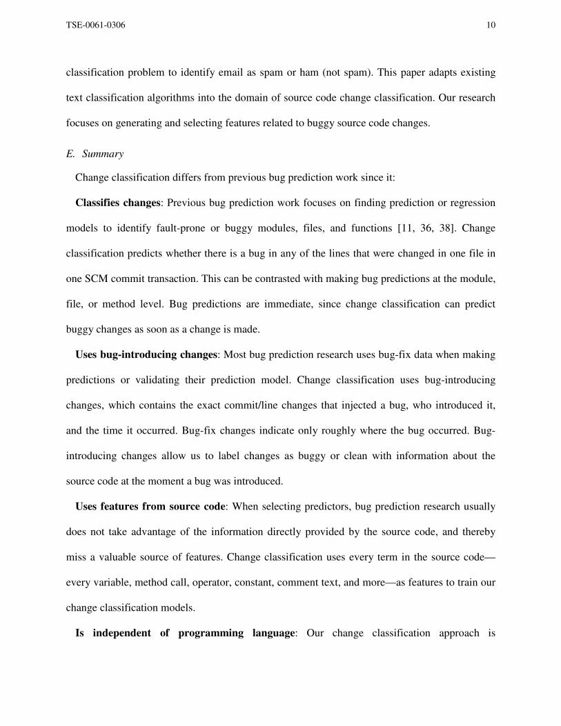
Figure 2 shows accuracy, buggy change recall, and buggy change precision of the 12 projects
using all features listed in Table 1.
TSE-0061-0306 25
Figure 2. Change classification accuracy, buggy change recall, and buggy change precision of 12 projects
using SVM and all features.
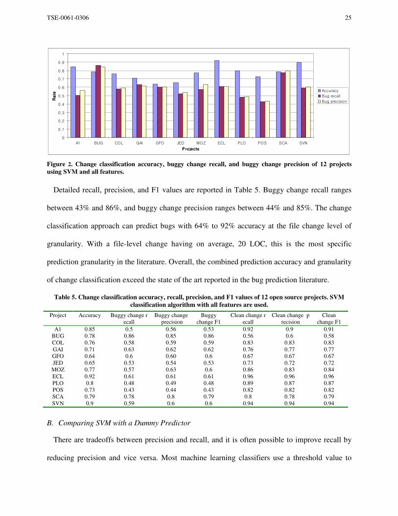
Detailed recall, precision, and F1 values are reported in Table 5. Buggy change recall ranges
between 43% and 86%, and buggy change precision ranges between 44% and 85%. The change
classification approach can predict bugs with 64% to 92% accuracy at the file change level of
granularity. With a file-level change having on average, 20 LOC, this is the most specific
prediction granularity in the literature. Overall, the combined prediction accuracy and granularity
of change classification exceed the state of the art reported in the bug prediction literature.
Table 5. Change classification accuracy, recall, precision, and F1 values of 12 open source projects. SVM
classification algorithm with all features are used.
Project Accuracy Buggy change r
ecall
Buggy change
precision
Buggy
change F1
Clean change r
ecall
Clean change p
recision
Clean
change F1
A1 0.85 0.5 0.56 0.53 0.92 0.9 0.91
BUG 0.78 0.86 0.85 0.86 0.56 0.6 0.58
COL 0.76 0.58 0.59 0.59 0.83 0.83 0.83
GAI 0.71 0.63 0.62 0.62 0.76 0.77 0.77
GFO 0.64 0.6 0.60 0.6 0.67 0.67 0.67
JED 0.65 0.53 0.54 0.53 0.73 0.72 0.72
MOZ 0.77 0.57 0.63 0.6 0.86 0.83 0.84
ECL 0.92 0.61 0.61 0.61 0.96 0.96 0.96
PLO 0.8 0.48 0.49 0.48 0.89 0.87 0.87
POS 0.73 0.43 0.44 0.43 0.82 0.82 0.82
SCA 0.79 0.78 0.8 0.79 0.8 0.78 0.79
SVN 0.9 0.59 0.6 0.6 0.94 0.94 0.94
B. Comparing SVM with a Dummy Predictor
There are tradeoffs between precision and recall, and it is often possible to improve recall by
reducing precision and vice versa. Most machine learning classifiers use a threshold value to
0
0.1
0.2
0.3
0.4
0.5
0.6
0.7
0.8
0.9
1
A1 BUG COL GAI GFO JED MOZ ECL PLO POS SCA SVN
P ro jectsP ro jectsP ro jectsP ro jects
Rate
Rate
Rate
Rate
Accuracy
Bug recall
Bug precision

TSE-0061-0306 26
classify instances. For example, SVM uses the distance between each instance and the
hyperplane to measure the weights of each instance. If an instance's weight is greater than the
threshold value, the instance belongs to class 1, otherwise it belongs to class 2. By lowering or
raising the threshold, it is possible to change recall and precision. Usually by lowering recall,
precision can be increased. For example, buggy change recall can easily go up to 100% by
predicting all changes as buggy, but the precision will be very low.
A recall-precision curve shows the trade-off between recall and precision. Figure 3 gives the
SVM classifier recall-precision curves of three selected projects, Bugzilla, Mozilla, and Scarab
(in solid lines). The curve for the Bugzilla project shows that the precision grows up to about 95%
(with 20% recall). For Mozilla and Scarab, the precision can reach 85-90% by lowering the
recall to 20%.
Figure 3. Buggy change recall-precision curves of selected 3 projects, Bugzilla, Mozilla, and Scarab using SVM.
Dummy classifier recall-precision curves are shown as dotted lines while the solid lines represent SVM classifier
recall-precision curves.
0
0.1
0.2
0.3
0.4
0.5
0.6
0.7
0.8
0.9
1
0 0.1 0.2 0.3 0.4 0.5 0.6 0.7 0.8 0.9 1
Precision
Re
ca
ll
Mozilla
Dummy
Mozilla
SVM
Scarab
Dummy
Bugzilla
Dummy
Scarab
SVM Bugzilla
SVM

TSE-0061-0306 27
How is SVM recall-precision better than other approaches, such as randomly guessing changes
(a dummy classifier) as buggy or clean? Since there are only two classes, the dummy classifier
may work well. For example, 73.7% of Bugzilla changes are buggy. By predicting all changes as
buggy, buggy recall would be 100% and precision would be 73.7%. Is this better than the results
when using SVM? The recall-precision curves of the dummy (dotted lines) and SVM (solid lines)
classifiers of three selected projects are compared in Figure 3. Precision for the Bugzilla dummy
classifier is stuck at 73.7%, while SVM precision grows up to 95% (with 20% recall). Similarly
for other projects, SVM can improve buggy change precision by 20% - 35%.
C. Correlation between Percentage of Bug Introducing Changes and Classification Accuracy
One observation that can be made from Table 1 is that the percentage of changes that are
buggy varies substantially among projects, ranging from 10.1% of changes for Eclipse to 73.7%
for Bugzilla. One explanation for this variance is the varying use of change log messages among
projects. Bugzilla and Scarab, being change tracking tool projects, have a higher overall use of
change tracking. It is likely that for those projects, the class of buggy changes also encompasses
other kinds of modifications. For these projects, change classification can be viewed as
successfully predicting the kinds of changes that result in change tracking tool entries.
Table 6. Correlation between the percentages of buggy changes and change classification performance.
Buggy % vs. accuracy Buggy % vs. buggy
change recall
Buggy % vs. buggy
change precision
Correlation -0.56 0.77 0.64
One question that arises is whether the percentage of buggy changes for a project affects
change classification performance such as accuracy, recall, and precision? A Pearson correlation
was computed between the percentage of buggy changes, and the measures of accuracy, recall,
and precision for the 12 projects analyzed in this paper. Table 6 lists the correlation values. A

TSE-0061-0306 28
correlation value of 1 indicates tight correlation, while 0 indicates no correlation. The values
show a weak negative correlation for accuracy, and weak, but not significant correlations for
buggy recall and precision.
VII. EVALUATION OF FEATURES AND FEATURE GROUPS
A. Change Classification Using Selected Feature Groups
This section evaluates the accuracy of different feature group combinations for performing
change classification. First, a classification model is trained using features from one feature
group, and then its accuracy and recall are measured. Following, a classification model is trained
using all feature groups except the one feature group, with accuracy and recall measured for this
case as well. In addition, an evaluation is made focusing on the combination of features extracted
solely from the source code (added delta, new revision source code, and deleted delta).
Table 7. Feature groups. The number of features in each feature group is shown for all analyzed projects.
Feature Group Number of features of projects
A1 BUG COL GAI GFO JED MOZ ECL PLO POS SCA SVN
Added Delta (A) 2024 2506 3811 2094 1895 2939 3079 2558 1540 3532 1290 2663 Deleted Delta (D) 1610 1839 3227 1956 1832 2352 2176 2200 1073 2995 836 2117 Directory/File Name (F) 93 66 559 39 242 377 105 456 221 472 106 195 Change Log (L) 1257 1124 869 1094 3970 431 959 53 2835 1161 650 2474 New Revision Source Code (N) 6330 4604 8814 3967 4481 7649 7320 10794 2671 14956 2697 7276 Metadata (M) 8 8 8 8 8 8 8 8 8 8 8 8 Complexity Metrics (C) 122 0 122 122 0 122 0 122 0 122 0 122
*Total 11445 10148 17411 9281 8996 13879 13648 16192 6127 23247 5710 14856
Extracted features are organized into groups based on their source. For example, features
extracted just from the change log messages are part of the Change Log (L) feature group. Table
7 provides a summary of feature groups and the number of features in each group. Software
complexity metrics were computed only for C/C++ and Java source code, since tools were not
available for computing these metrics for Java Script, Perl, PHP, and Python.
Figure 4 shows the change classification accuracy for the Mozilla and Eclipse projects using
various feature group combinations. The abbreviations for each feature group are shown in Table

TSE-0061-0306 29
7. An abbreviation means only the feature group is used for classification. For example, ‘D’
means only features from the Deleted Delta group were used. The ‘~’ mark indicates the
corresponding feature group is excluded. For example, ‘~D’ means all features were used except
for D (Deleted delta). The feature group “AND” is the combination of all source code feature
groups (A, N, and D). The accuracy trend of the two projects is different, but they share some
properties. For example, the accuracy using only one feature group is lower than using multiple
feature groups.
Figure 4. Feature group combination accuracy for Eclipse and Mozilla using SVM. Complexity metrics (C)
are not available for Mozilla, so ~C and C are omitted.
The average accuracy of 12 open source projects using various feature combinations is shown
in Figure 5. Using a feature combination of only source code (A, N, and D combined) leads to a
relatively high accuracy, while using only one feature group from the source code, such as A, N,
or D individually, does not lead to high accuracy. Using only ‘L’ (change log features) leads to
the worst accuracy.
0
0.1
0.2
0.3
0.4
0.5
0.6
0.7
0.8
0.9
1
~A A All AND ~L L ~C C ~D D ~F F ~M M ~N N
Feature Group Combination
Accu
racy
Eclipse
Mozilla

TSE-0061-0306 30
Figure 5. Average feature group combination accuracy across the 12 analyzed projects using SVM
After analyzing the combinations of feature groups, the feature combination that yields the best
accuracy and best recall for each project are identified, as shown in Table 8. The results indicate
that there is no feature combination that works best across projects, and that frequently the
feature group providing the best accuracy is not the same as the feature group providing the best
buggy recall. A practical implication of this data is that each project has the opportunity to
engage in a project-specific feature selection process that can optimize for either accuracy or
recall, but often not both simultaneously.
Table 8. Feature group combination yielding the best classification accuracy and buggy change recall using
SVM. The feature group listed in parentheses yields the best accuracy/buggy change recall.
Projects A1 BUG COL GAI GFO JED MOZ ECL PLO POS SCA SVN
Best accuracy 0.86
(~F)
0.79
(~M)
0.77
(~M)
0.72
(~D)
0.65
(~L)
0.68
(~C)
0.77
(ALL)
0.93
(~N)
0.81
(~D)
0.76
(C)
0.81
(~F)
0.9
(ALL)
Best buggy
change recall
0.57
(ALL)
0.98
(M)
0.61
(~M)
0.63
(ALL)
0.62
(~L)
0.57
(~C)
0.57
(ALL)
0.63
(~F)
0.51
(~D)
0.43
(ALL)
0.8
(~D)
0.6
(~M)
B. Important Individual Features
While the feature group importance provides some insight into the relative importance of
groups of features, it does not say anything about individual features. Which features are the
most important within a given project?
0.69
0.7
0.71
0.72
0.73
0.74
0.75
0.76
0.77
0.78
0.79
0.8
~A A All AND ~L L ~C C ~D D ~F F ~M M ~N N
Feature Group CombinationFeature Group CombinationFeature Group CombinationFeature Group Combination
Accura
cy
Accura
cy
Accura
cy
Accura
cy

TSE-0061-0306 31
Using the chi-squared measure, all features are ranked individually. Additionally, the
distribution of each feature in buggy and clean changes is computed to decide whether the
corresponding feature contributes more to buggy or clean change classification. The top 5 ranked
individual features in each feature group are determined, and presented in Table 9. Each box lists
the top 5 ranked features within a feature group, for a given project. Each individual feature is
listed, along with its overall numerical rank among the total set of features available for that
project. The + and – before the rank indicate whether the feature is contributing to the buggy (+)
or clean (-) change class.
Table 9. Top five ranked individual features in each feature group. Numbers in parentheses indicate the overall
rank (computed using a Chi-square measure) of a feature’s importance among all features. A ‘+’ sign indicates the
feature contributes to buggy changes, and a ‘–’ sign indicates the feature contributes to clean changes. The △ mark
beside a complexity metric indicates it is a delta metric.
Bugzilla Eclipse Plone
Complexity
metrics N/A
SumEssential(-117),
△CountLineBlank(+228),
CountStmtDecl(-417),
CountLineComment(-419),
CountLineCodeDecl(-420)
N/A
Change
Log
fix(+345), comments
(-351), correcting(-414),
patch(+480), ability(- 492)
fix(+386), for(+398), 18(+961),
3249(+962),
1(- 1795)
action(+396), beautified(+576),
catch(+577), categories(+578),
global(+579)
Metadata
changed loc(+1), loc(+2), bug
count(+3), time(-9), change
count(+43)
time(+74), changed loc(+88), bug
count(+104), days(-137), change log
length(-142)
changed loc(+21), bug count(+140),
loc(+274), time(-456), author(+676)
New
Source
order(+4), b(+7), bit(+8),
ok(+10), used(+11)
flowinfo(+1), analysecode(+2),
flowcontext(+3), slow(+4),
iabstractsynt(+6)
globals(-2), security(+3), not(+4),
accesscontrol(+5), aq(+6)
Added
Delta
if(+5), my(+6), value(+15),
not(+22), sendsql(+26)
codestream(+12),
recordpositionsfrom(+8),
belongsto(+24), complete(+25),
jobfamily(+26)
self(+1), def(+26), %(+40),
raise(+46), log(+50)
Deleted
Delta
name(+153), value(+281),
my(+300), fetchsqldata(+326),
sendsql(+349)
codestream(+14), public(+15),
recordpositionsfrom(+19), return(+21),
this(+22)
self(+14), %(+47), log(+55), def(+107),
else(+143)
Directory/
File name
relation(-219), set(-220),
move(-375), createattachment(-
490), export(-491)
ast(+5), compiler(+47),
statement(+108), core
(- 116), model(-214)
tool(+10), scripts(-154), edit(-340),
form(-411), folder(+470)
For example, in the Bugzilla project in the Added Delta feature group, the keyword “if” is
listed as the top feature within the group, and is the 5th
most important individual feature overall.
Compared to traditional bug prediction research that tends to use software metrics to determine

TSE-0061-0306 32
bugs in software, the most important individual features presented above seem to have limited
utility for constructing causal models of what causes a bug. A general, cross-project causal
model of bug injection just cannot explain why “if” is a strong feature for Bugzilla, while “self”
is a strong feature for Plone. One explanation is that these are statistically correlated features
computed for each project, and hence there should not be any expectation of a deeper model. The
individual important features are deeply project-specific, indicating that no cross-project
classification model can be developed. It is just not possible to train a classifier using these
feature types on one project, then apply it to another project, and obtain any kind of reasonable
accuracy, precision, or recall.
One interesting question is whether the committing developer is predictive for bugginess.
Based on this data, the short answer is “no”, not for change classification. In Table 9 above, only
one project, Plone, lists author as a top 5 feature within the metadata feature group, and it is
ranked low, at 676. One explanation is that even bug-prone developers tend to make more clean
changes than buggy changes. If, hypothetically, a developer made 85% clean changes and 15%
buggy changes, they might be perceived by their peers to be a bug-prone developer, while the
change classifier would view this same developer as a strong feature for predicting clean changes.
An intriguing potential extension of change classification would be to train one change classifier
for each developer on a project, and then perform developer-specific bug prediction. Developers
are expected to have developer-specific patterns in their bug introducing changes, and this might
improve the performance of change classification. This remains future work.

TSE-0061-0306 33
VIII. DISCUSSION
This section discusses possible applications of change classification, and provides additional
interpretation of the results. This section ends with some discussion on the limitations of our
experiments.
A. Potential Applications of Change Classification
Right now, the buggy change classifier operates in a lab environment. However, it could
potentially be put into use in various ways:
• A commit checker: The classifier identifies buggy changes during commits of changes to
a SCM system, and notifies developers of the results. The bug prediction in the commit
checker is immediate, and makes it easy for developers to inspect the change just made.
• Potential bug indicator during source code editing: We have shown that features from
source code (A, N, D) have discriminative power (see Figure 5). That is, just using features
from source code, it is possible to perform accurate bug classification. This implies that a
bug classifier can be embedded in a source code editor. During the source code editing
process, the classifier could monitor source code changes. As soon as the cumulative set of
changes made during an editing session leads the classifier to make a bug prediction, the
editor can notify the developer. A proof of concept implementation of this idea using the
Eclipse IDE is reported in [27].
• Impact on the software development process: Results from the change classifier could
be integrated into the software development process. After committing a change, a
developer receives feedback from the classifier. If the classifier indicates it was a buggy
change, this could trigger an automatic code inspection on the change by multiple
engineers. After the inspection, the developer commits a modified change and receives

TSE-0061-0306 34
more feedback. If this approach is effective in finding bugs right away, it could
significantly reduce the number of latent bugs in a software system.
B. Issues of Change Classification
A software project that records its changes in an SCM system, has approximately 100 or more
SCM commits, and has some record of which commits fix bugs, may have the change
classification technique used on it.
Several issues arise when extracting features from an existing project. First, an examination of
change log messages is required to determine how best to determine the bug fix changes. The
best set of keywords depends on how each project has used their SCM log messages in the past.
For projects that consistently use a change tracking system, data may need to be extracted from
this system as well.
Another concern is ensuring the memory capacity of the machine performing classification is
not exceeded, as this leads to excessive swapping to disk, and reduced performance. Two
techniques can be used to reduce memory usage. The range of revisions used to train the
classifier can be reduced; this was the case in the current paper with the Eclipse and JEdit
projects. The project can also be subdivided into smaller modules, such as considering only a
specific subdirectory within a large project. A single, moderately high-end workstation computer
should be sufficient for performing change classification work, and hence hardware costs for
implementing the technique are modest.
An SVM classifier generally works well using all feature groups available for a project. If time
is available, a given project can consider performing a feature group sensitivity analysis, of the
type described in Section VII. This permits the use of the most accurate feature groups for the
current project, usually resulting in a small gain in performance. Another consideration is

TSE-0061-0306 35
whether an existing complexity metric computation tool is available. Change classification can
provide accurate results without the use of complexity metrics as a feature, however, complexity
metrics are sometimes the most accurate single class of feature.
In an ongoing project, the SVM classifier will need to be periodically retrained to
accommodate data from new project changes. If a project is small enough, training an SVM
could be performed nightly, at the end of the workday. On larger projects, the SVM could be
retrained weekly.
All in all, we expect that change classification will assist developers in identifying those
changes that are most likely to contain bugs—and thus increase quality, reduce effort, or both.
C. Minimum Change Numbers for Classifier Training
The results presented in this paper use changes in 500 (or 250 revisions) to train and evaluate
an SVM classifier. This raises the question of how many revisions or changes are required to
train an SVM classifier to yield reasonable classification performance. To answer this question,
subsets of changes are used to train and evaluate an SVM classifier with all features. To begin,
only the first 10 changes are used to train and evaluate a classifier. Next, the first 20 changes are
used. In the same way, the number of changes is increased by 10 and then used to train and
evaluate an SVM classifier.

TSE-0061-0306 36
Figure 6. Number of changes used to train and evaluate an SVM classifier and their corresponding accuracy of selected
projects: Apache, Bugzilla, GForge, Mozilla, and SVN.
Figure 6 shows accuracies of selected projects by using various numbers of changes. Two
conclusions can be drawn from this. First, after approximately 100 changes predictive accuracy
is generally close to steady-state values. There is still some churn in accuracy from changes 100
to 200, but the accuracy does not have dramatic swings (for example, no +/- 20% deviations)
after this point. Accuracies settle down to steady-state values after 200 changes for most projects.
It thus appears that change classification using an SVM classifier is usable as a bug prediction
technique once a project has logged 100 changes, though with some variability in predictive
accuracy for the next 100 changes until accuracy values ready steady-state. Due to this, if change
classification is to be used on a new software project, it is probably best adopted towards the
middle or end of the initial coding phase, once sufficient changes have been logged and initial
testing efforts have begun to reveal project bugs. Any project that has already had at least one
release would typically be able to adopt change classification at any time.
0
10
20
30
40
50
60
70
80
90
100
10
40
70
100
130
160
190
220
250
280
310
340
370
400
430
460
490
520
550
580
610
640
670
700
730
760
790
Number of changes
Accura
cy
Apache
Bugzilla
GForge
Mozilla
SVN

TSE-0061-0306 37
D. Threats to Validity
There are five major threats to the validity of this study.
Systems examined might not be representative. 12 systems are examined, more than any
other work reported in the literature. In spite of this, it is still possible that we accidentally chose
systems that have better (or worse) than average bug classification accuracy. Since we
intentionally only chose systems that had some degree of linkage between change tracking
systems and the text in the change log (so we could determine fix inducing changes), we have a
project selection bias. This is most evident in the data from Bugzilla and Scarab, where the fact
that they are change tracking systems led to a higher than normal ratio of buggy to clean changes.
Systems are all open source. The systems examined in this paper all use an open source
development methodology, and hence might not be representative of all development contexts. It
is possible that the stronger deadline pressure, different personnel turnover patterns, and different
development processes used in commercial development could lead to different buggy change
patterns.
Bug fix data is incomplete. Even though we selected projects that have change logs with good
quality, we still are only able to extract a subset of the total number of bugs (typically only 40%-
60% of those reported in the bug tracking system). Since the quality of change logs varies across
projects, it is possible that the output of the classification algorithm will include false positive
and false negatives. It is currently unclear what impact lower quality change logs has on the
classification results.
Bug introducing data is incomplete. The SZZ algorithm used to identify bug-introducing
changes has limitations: it cannot find bug introducing changes for bug fixes that only involve
the deletion of source code. It also cannot identify bug-introducing changes caused by a change
made to a file different from the one being analyzed. It is also possible to miss bug-introducing

TSE-0061-0306 38
changes when a file changes its name, since the algorithm does not track such name changes.
Requires initial change data to train a classification model. As discussed in Section C, the
change classification technique requires about 100 changes to train a project specific
classification model before predictive accuracy achieves a “usable” level of accuracy.
Use of bug tracking systems for tracking new functionalities. In two of the systems
examined, Bugzilla and Scarab, the projects used bug tracking systems to also track new
functionality additions to the project. For these projects, the meaning of a bug tracking identifier
in the change log message either means a bug was fixed, or a new functionality added. This
substantially increases the number of changes flagged as bug fixes. For these systems, the
interpretation of a positive classification output is a change that is either buggy or a new
functionality. When using this algorithm, care needs to be taken to understand the meaning of
changes identified as bugs, and, wherever possible, to ensure that only truly buggy changes are
flagged as being buggy.
IX. CONCLUSION AND OPEN ISSUES
If a developer knows that a change she just made contains a bug, she can use this information
to take steps to identify and fix the potential bug in the change before it leads to a bug report.
This paper has introduced a new bug prediction technique that works at fine granularity, an
individual file level change, and has accuracy comparable to the best existing bug prediction
techniques in the literature (78%, on average). Features gathered only from source code have
strong discriminative power, suggesting the possibility of embedding the classification algorithm
into integrated development environments for bug prediction during editing sessions. Developers
can benefit from focused and prompt prediction of buggy changes, receiving this prediction
either while they are editing source code or right after a change submission.

TSE-0061-0306 39
This work is the first to classify file changes as buggy or clean using the combination of
change information features and source code terms. Additionally, this work provides an
evaluation of the relative contributions of various feature groups for change classification.
Although these experimental results are encouraging, there are still several open issues in this
work, including:
� Exploring on-line machine learning algorithms to learn and update a classification model
as the project progresses and using it to predict future changes.
� Generating more features from change information and exploring various ways to
extract features, such as latent semantic analysis [22].
� Deep analysis on the individual features to identify common bug-prone code patterns or
causality of bugs.
� Applying or modifying existing machine learning algorithms to achieve better prediction
accuracy, precision, and recall [9].
� Finally, use in ongoing software projects to see how developers exploit bug
classification information to perform bug reducing interventions in their software.
Overall, we expect that future approaches will see software history not only as a series of
revisions and changes, but also as a series of successes and failures—and as a source for
continuous awareness and improvement. Change classification is a first step in this direction.
ACKNOWLEDGMENT
We thank David P. Helmbold for his guidance and insight on the machine learning algorithms
for file change classifications. We thank Kai Pan and Mark Slater for their valuable feedback on
this paper. We especially thank Kevin Greenan and the Storage Systems Research Center at
UCSC for allowing the use of their cluster for our research. Comments by the anonymous

TSE-0061-0306 40
reviewers were very helpful in improving the paper, and are greatly appreciated.
REFERENCES
[1] E. Alpaydin, Introduction to Machine Learning: The MIT Press, 2004.
[2] G. Antoniol, G. Casazza, and A. Cimitile, "Traceability Recovery by Modelling Programmer Behaviour," Proc. of 7th Working
Conference on Reverse Engineering, Brisbane, Queensland, Australia, pp. 240-247., 2000.
[3] J. Anvik, L. Hiew, and G. C. Murphy, "Who Should Fix This Bug?" Proc. of 2006 International Conference on Software Engineering
(ICSE 2006), Shanghai, China, pp. 361-370, 2006.
[4] J. Bevan, E. J. Whitehead, Jr., S. Kim, and M. Godfrey, "Facilitating Software Evolution with Kenyon," Proc. of the 2005 European
Software Engineering Conference and 2005 Foundations of Software Engineering (ESEC/FSE 2005), Lisbon, Portugal, pp. 177-186,
2005.
[5] Y. Brun and M. D. Ernst, "Finding Latent Code Errors via Machine Learning over Program Executions," Proc. of 26th International
Conference on Software Engineering (ICSE 2004), Scotland, UK, pp. 480-490, 2004.
[6] D. Cubranic and G. C. Murphy, "Hipikat: Recommending pertinent software development artifacts," Proc. of 25th International
Conference on Software Engineering (ICSE 2003), Portland, Oregon, pp. 408-418, 2003.
[7] M. Fischer, M. Pinzger, and H. Gall, "Populating a Release History Database from Version Control and Bug Tracking Systems," Proc.
of 19th International Conference on Software Maintenance (ICSM 2003), Amsterdam, The Netherlands, pp. 23-32, 2003.
[8] C. Flanagan, K. R. M. Leino, M. Lillibridge, G. Nelson, J. B. Saxe, and R. Stata, "Extended Static Checking for Java," Proc. of the
ACM SIGPLAN 2002 Conference on Programming Language Design and Implementation, Berlin, Germany, pp. 234-245, 2002.
[9] Y. Freund and R. E. Schapire, "A Short Introduction to Boosting," Journal of Japanese Society for Artificial Intelligence, vol. 14, no.
5, pp. 771-780, 1999.
[10] G. A. Di Lucca, M. Di Penta, and S. Gradara, "An Approach to Classify Software Maintenance Requests," Proc. of 18th International
Conference on Software Maintenance (ICSM 2002), Montréal, Canada, pp. 93-102, 2002.
[11] T. L. Graves, A. F. Karr, J. S. Marron, and H. Siy, "Predicting Fault Incidence Using Software Change History," IEEE Transactions
on Software Engineering, vol. 26, no. 7, pp. 653-661, 2000.
[12] T. Gyimothy, R. Ferenc, and I. Siket, "Empirical Validation of Object-Oriented Metrics on Open Source Software for Fault
Prediction," IEEE Transactions on Software Engneering, vol. 31, no. 10, pp. 897-910, 2005.
[13] A. E. Hassan and R. C. Holt, "The Top Ten List: Dynamic Fault Prediction," Proc. of 21st International Conference on Software
Maintenance (ICSM 2005), Budapest, Hungary, pp. 263-272, 2005.
[14] T. Joachims, "Text Categorization with Support Vector Machines: Learning with Many Relevant Features," Proc. of ECML 98, 10th
European Conference on Machine Learning, Chemnitz, Germany, pp. 137-142, 1998.
[15] T. M. Khoshgoftaar and E. B. Allen, "Ordering Fault-Prone Software Modules," Software Quality Control Journal, vol. 11, no. 1, pp.
19-37, 2003.
[16] T. M. Khoshgoftaar and E. B. Allen, "Predicting the Order of Fault-Prone Modules in Legacy Software," Proc. of The Ninth
International Symposium on Software Reliability Engineering, Paderborn, Germany, pp. 344-353, 1998.
[17] S. Kim, K. Pan, and E. J. Whitehead, Jr., "Memories of Bug Fixes," Proc. of the 2006 ACM SIGSOFT Foundations of Software
Engineering (FSE 2006), Portland, Oregon, pp. 35 - 45, 2006.
[18] S. Kim, T. Zimmermann, E. J. Whitehead, Jr., and A. Zeller, "Predicting Bugs from Cached History," Proc. of the 29th International
Conference on Software Engineering (ICSE 2007), Minneapolis, USA, pp. 489-498, 2007.
[19] R. Krovetz, S. Ugurel, and C. L. Giles, "Classification of Source Code Archives," Proc. of the 26th International ACM SIGIR
Conference on Research and Development in Information Retrieval, Toronto, Canada, pp. 425-426, 2003.
[20] A. Kuhn, S. Ducasse, and T. Girba, "Enriching Reverse Engineering with Semantic Clustering," Proc. of 12th Working Conference on
Reverse Engineering (WCRE 2005), Pittsburgh, Pennsylvania, USA, pp. 133-142, 2005.
[21] R. Kumar, S. Rai, and J. L. Trahan, "Neural-Network Techniques for Software-quality Evaluation," Proc. of 1998 Reliability and
Maintainability Symposium, Anaheim, CA, pp. 155-161, 1998.
[22] T. K. Landauer, P. W. Foltz, and D. Laham, "Introduction to Latent Semantic Analysis," Discourse Processes, vol. 25, pp. 259-284,
1998.
[23] D. Lewis, Y. Yang, T. Rose, and F. Li, "RCV1: A New Benchmark Collection for Text Categorization Research," Journal of Machine
Learning Research, vol. 5, pp. 361-397, 2004.
[24] Z. Li and Y. Zhou, "PR-Miner: Automatically Extracting Implicit Programming Rules and Detecting Violations in Large Software
Code," Proc. of the 2005 European Software Engineering Conference and 2005 Foundations of Software Engineering (ESEC/FSE
2005), Lisbon, Portugal, pp. 306 - 315, 2005.
[25] B. Livshits and T. Zimmermann, "DynaMine: Finding Common Error Patterns by Mining Software Revision Histories," Proc. of the
2005 European Software Engineering Conference and 2005 Foundations of Software Engineering (ESEC/FSE 2005), Lisbon,
Portugal, pp. 296-305, 2005.
[26] J. Lyle and M. Weiser, "Automatic Program Bug Location by Program Slicing," Proc. of 2nd International Conference on Computers
and Applications, pp. 877-883, 1987.
[27] J. Madhavan and E. J. Whitehead, Jr., "Predicting Changes Inside an Integrated Development Environment," Proc. of 2007 Eclipse
Technology Exchange Workshop, Montreal, Canada, 2007.
[28] J. I. Maletic and N. Valluri, "Automatic Software Clustering via Latent Semantic Analysis," Proc. of 14th IEEE International
Conference on Automated Software Engineering (ASE'99), Cocoa Beach, Florida, USA, pp. 251, 1999.
[29] A. Marcus and J. I. Maletic, "Recovering Documentation-to-Source-Code Traceability Links using Latent Semantic Indexing," Proc.
of the 25th International Conference on Software Engineering, Portland, Oregon, pp. 125-135, 2003.
[30] T. Menzies, J. Greenwald, and A. Frank, " Data Mining Static Code Attributes to Learn Defect Predictors," IEEE Trans. Software
Engineering, vol. 33, no. 1, pp. 2-13, 2007.

TSE-0061-0306 41
[31] O. Mizuno and T. Kikuno, "Training on Errors Experiment to Detect Fault-prone Software Modules by Spam Filter," Proc. of the
2007 European Software Engineering Conference and 2007 Foundations of Software Engineering (ESEC/FSE 2007), Dubrovnik,
Croatia, pp. 405 - 414, 2007.
[32] A. Mockus and L. G. Votta, "Identifying Reasons for Software Changes Using Historic Databases," Proc. of 16th International
Conference on Software Maintenance (ICSM 2000), San Jose, California, USA, pp. 120-130, 2000.
[33] A. Mockus and D. M. Weiss, "Predicting Risk of Software Changes," Bell Labs Technical Journal, vol. 5, no. 2, pp. 169-180, 2002.
[34] D. C. Montgomery, G. C. Runger, and N. F. Hubele, Engineering Statistics: Wiley, 2001.
[35] A. W. Moore, "Cross-Validation," 2005, http://www.autonlab.org/tutorials/overfit.html.
[36] N. Nagappan and T. Ball, "Use of Relative Code Churn Measures to Predict System Defect Density," Proc. of 27th International
Conference on Software Engineering (ICSE 2005), Saint Louis, Missouri, USA, pp. 284-292, 2005.
[37] D. J. Newman, S. Hettich, C. L. Blake, and C. J. Merz, "UCI Repository of machine learning databases," 1988,
http://www.ics.uci.edu/~mlearn/MLRepository.html.
[38] T. J. Ostrand and E. J. Weyuker, "The Distribution of Faults in a Large Industrial Software System," Proc. of the 2002 ACM SIGSOFT
International Symposium on Software Testing and Analysis, Roma, Italy, pp. 55-64, 2002.
[39] T. J. Ostrand, E. J. Weyuker, and R. M. Bell, "Predicting the Location and Number of Faults in Large Software Systems," IEEE
Transactions on Software Engineering, vol. 31, no. 4, pp. 340-355, 2005.
[40] T. J. Ostrand, E. J. Weyuker, and R. M. Bell, "Where the Bugs Are," Proc. of 2004 ACM SIGSOFT International Symposium on
Software Testing and Analysis, Boston, Massachusetts, USA, pp. 86-96, 2004.
[41] K. Pan, S. Kim, and J. E. James Whitehead, "Bug Classification Using Program Slicing Metrics," Proc. of the Sixth IEEE
International Workshop on Source Code Analysis and Manipulation (SCAM 2006), Philadelphia, PA, 2006.
[42] M. D. Penta, S. Gradara, and G. Antoniol, "Traceability Recovery in RAD Software Systems," Proc. of the 10th IEEE International
Workshop on Program Comprehension, Paris, France, pp. 207-216., 2002.
[43] B. Raskutti, H. L. Ferrá, and A. Kowalczyk, "Second Order Features for Maximizing Text Classification Performance," Proc. of 12th
European Conference on Machine Learning, Freiburg, Germany, pp. 419-430, 2001.
[44] Scientific Toolworks, "Maintenance, Understanding, Metrics and Documentation Tools for Ada, C, C++, Java, and FORTRAN," 2005,
http://www.scitools.com/.
[45] S. Scott and S. Matwin, "Feature Engineering for Text Classification," Proc. of the Sixteenth International Conference on Machine
Learning, Bled, Slovenia, pp. 379-388, 1999.
[46] F. Sebastiani, "Machine Learning in Automated Text Categorization," ACM Computing Surveys, vol. 34, no. 1, pp. 1-47, 2002.
[47] J. Śliwerski, T. Zimmermann, and A. Zeller, "When Do Changes Induce Fixes?" Proc. of Int'l Workshop on Mining Software
Repositories (MSR 2005), Saint Louis, Missouri, USA, pp. 24-28, 2005.
[48] J. C. Spohrer, E. Soloway, and E. Pope, "Where the Bugs Are," Proc. of the SIGCHI Conference on Human Factors in Computing
Systems, San Francisco, California, USA, pp. 47-53, 1985.
[49] V. N. Vapnik, The Nature of Statistical Learning Theory: Springer-Verlag, 1995.
[50] Wikipedia, "CamelCase," 2005, http://en.wikipedia.org/wiki/CamelCase.
[51] C. C. Williams and J. K. Hollingsworth, "Automatic Mining of Source Code Repositories to Improve Bug Finding Techniques," IEEE
Trans. Software Engineering, vol. 31, no. 6, pp. 466-480, 2005.
[52] I. H. Witten and E. Frank, Data Mining: Practical Machine Learning Tools and Techniques (Second Edition): Morgan Kaufmann,
2005.
[53] L. Zhang, J. Zhu, and T. Yao, "An Evaluation of Statistical Spam Filtering Techniques," ACM Transactions on Asian Language
Information Processing (TALIP), vol. 3, no. 4, pp. 243-269, 2004.
[54] Z. Zheng, X. Wu, and R. Srihari, "Feature selection for text categorization on imbalanced data," ACM SIGKDD Explorations
Newsletter, vol. 6, no. 1, pp. 80-89, 2004.
[55] T. Zimmermann and P. Weißgerber, "Preprocessing CVS Data for Fine-Grained Analysis," Proc. of Int'l Workshop on Mining
Software Repositories (MSR 2004), Edinburgh, Scotland, pp. 2-6, 2004.
[56] T. Zimmermann, P. Weißgerber, S. Diehl, and A. Zeller, "Mining Version Histories to Guide Software Changes," IEEE Trans.
Software Engineering, vol. 31, no. 6, pp. 429-445, 2005.
Sunghun Kim is a postdoctoral associate at the Massachusetts Institute of Technology. He received his PhD in Computer Science from the
University of California, Santa Cruz in 2006. His main research interests are dynamic bug prediction and identifying common bug
patterns by mining software repositories.
E. James Whitehead, Jr. (M’93) is an Associate Professor of Computer Science at the University of California, Santa Cruz. He received his
PhD in Information and Computer Science in 2000 from the University of California, Irvine, and his BS in Electrical Engineering
from the Rensselaer Polytechnic Institute in 1989. His research interests include software evolution, software design, application layer
network protocols, collaborative authoring, computer game design and hypertext systems.
Yi Zhang (M'06) is an Assistant Professor at the University of California Santa Cruz. She received her Ph.D. and M.S. from Carnegie Mellon
University. She was born in 1976 in Chengdu, China.