Classifying rangeland vegetation type and coverage from NDVI time

Classifying rangeland vegetation type and coverage from NDVI timeseries using Fourier Filtered Cycle Similarity

R. GEERKEN*, B. ZAITCHIK and J. P. EVANS

Department for Geology and Geophysics, Yale University, New Haven, Connecticut

06520, USA

(Received 14 June 2004; in final form 30 March 2005 )

We present a method for a supervised classification of Normalized Difference

Vegetation Index (NDVI) time series that identifies vegetation type and vegetation

coverage, absolute in %coverage or relative to a reference NDVI cycle. The shape

of the NDVI cycle, which is diagnostic for certain vegetation types, is our primary

classifier. A Discrete Fourier Filter is applied to time series data in order to

minimize the influence of high-frequency noise on class assignments. Similarity

between filtered NDVI cycles is evaluated using a linear regression technique. The

correlation coefficients calculated between the Fourier filtered reference cycle and

likewise filtered target cycles describe the similarity of their phenology, and the

corresponding regression coefficients are an expression of coverage relative to the

reference. The regression coefficients are correlated with field measured vegetation

coverage. The Fourier Filtered Cycle Similarity method (FFCS) compensates

phenological shifts, which are typical in areas with a strong climate gradient, and

prevents the break-up of classes of identical vegetation types on the basis of

vegetation coverage. Some other advantages compared to traditional unsupervised

classifications are: synoptic visualization of vegetation type and coverage

variation, independence from scene statistics, and consistent classification of

biophysical characteristics only, without rock/soil reflectance dominating class

assignment as it often does in unsupervised classifications of sparsely vegetated

areas. Using the FFCS classification we differentiated a total of five rangeland

vegetation types for the area of Syria including their intra-class coverage variation.

Classified classes are dominated by one of two shrub types, one of two annual grass

types or a bare soil/sparsely vegetated type.

1. Introduction

The most common approach in classifying composited time series of the Normalized

Difference Vegetation Index (NDVI) is unsupervised classification, where pixels are

assigned to a user-defined number of classes based on a cluster analysis. The

Iterative Self-Organizing Data Analysis Technique (ISODATA) and the k-means

classifications (Tou and Gonzalez 1974) are probably the most widely used cluster

algorithms in satellite data analyses. Though these techniques offer certain

advantages, particularly where no field information is available, their results may

show inaccuracies and limitations in applicability. These may be caused by an over-

segmentation, under-segmentation, or by their dependency on scene statistics, which

makes results of cluster analyses spatially and temporally not comparable. Further

*Corresponding author. Email: [email protected]

International Journal of Remote Sensing

Vol. 26, No. 24, 20 December 2005, 5535–5554

International Journal of Remote SensingISSN 0143-1161 print/ISSN 1366-5901 online # 2005 Taylor & Francis

http://www.tandf.co.uk/journalsDOI: 10.1080/01431160500300297

limitations can be related to the clustering of pixels based on the most different

characteristics, making a consistent class description impossible. Clustering may be

the expression of different vegetation types but also of differences in background

reflectance (particularly important in sparsely vegetated areas), of variations in

vegetation coverage, or of climate induced phenological shifts. Accordingly, class

descriptions tend to have little meaning, and especially important for the rangelands,

typical intra-class coverage variations are not reflected. Due to these shortcomings

unsupervised classification does not fully exploit the biophysical information

contained in NDVI time series.

The accurate assessment of rangeland vegetation covers, in terms of their

productivity, their vulnerability to drought, or their degree of degradation, requires

information about the dominant vegetation types including their spatial variations in

coverage (LeHouerou 1996). With regard to vegetation type, two essential separations

are those between woody shrubs and annuals and between palatable and unpalatable

shrubs. This clearly emphasizes the need for a classification technique that gives more

consideration to the biophysical information contained in NDVI time series,

incorporating both vegetation type and spatial intra-class coverage variability.

Therefore, our study focused on the development of a classification technique that

identifies functional vegetation groups including their coverage variation. Particular

importance was given to those vegetation characteristics that define ecosystem

health. These include vegetation characteristics like palatability, degraded or

undegraded, annuals or perennials, the protection a vegetation type provides against

soil erosion as well as vegetation related hydro-meteorological parameters like run-

off, infiltration, and evapotranspiration. Many of the cited plant parameters find

expression in the plants’ phenology (Aguiar et al. 1996, Holmes and Rice 1996) and

by this in their NDVI cycle. A suitable classification technique, therefore, must give

more emphasis to the identification of similarities in the plants’ phenology than to

their absolute NDVI values.

NDVI cycles of identical vegetation types may well vary in absolute NDVI values

(amplitude), due to variations in coverage or vigour, but they will still share certain

poly-line characteristics because they have the same phenology. As shown by Geerken

et al. (2004), certain rangeland vegetation types show differences in their seasonal

growing patterns, inducing NDVI cycles of a diagnostic shape. In order to give more

consideration to the vegetation-diagnostic phenological details contained in the shape

of the NDVI cycle and to possible coverage variations, we developed an approach

based on linear regression technique that uses the similarity between phenological

cycles as its primary classifier. Because our approach uses linear regression which

assumes a normal distribution (here: normally distributed NDVI cycles), we restrict

our study to semi-arid and arid vegetation covers that usually fulfil such a

precondition. In more humid climates, plateau shaped vegetation cycles with an

extended period of high NDVI values become more ubiquitous and our method is

likely to fail. However, as long as the cycles fulfil the normal distribution requirement

it does not exclude the method’s application to vegetation covers of humid climates.

The procedures and algorithms described in the following were tested and applied

to an NDVI time series of Systeme Probatoire d’Observation de la Terre (SPOT)

VEGETATION data (Instrument VGT1, Type S10) covering the rangelands of

Syria (figure 1). The data are a subset of the West Asia tile with a spatial resolution

of 1 km. The NDVI layers of SPOT VEGETATION are composited from data

acquired over a 10-day period, where the 1st, the 11th, and the 21st of each month

5536 R. Geerken et al.

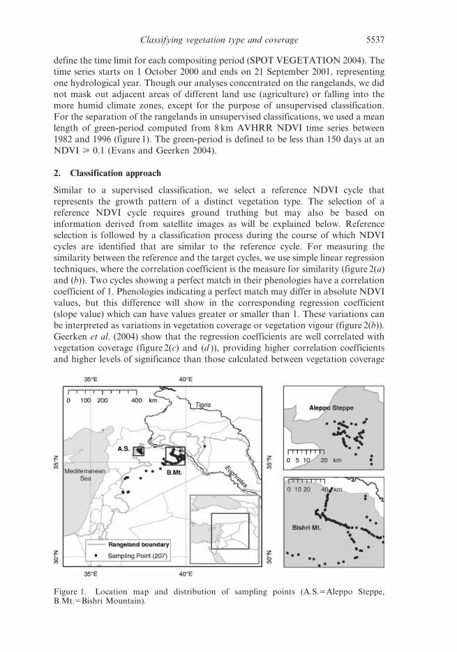
define the time limit for each compositing period (SPOT VEGETATION 2004). The

time series starts on 1 October 2000 and ends on 21 September 2001, representing

one hydrological year. Though our analyses concentrated on the rangelands, we did

not mask out adjacent areas of different land use (agriculture) or falling into the

more humid climate zones, except for the purpose of unsupervised classification.

For the separation of the rangelands in unsupervised classifications, we used a mean

length of green-period computed from 8 km AVHRR NDVI time series between

1982 and 1996 (figure 1). The green-period is defined to be less than 150 days at an

NDVI > 0.1 (Evans and Geerken 2004).

2. Classification approach

Similar to a supervised classification, we select a reference NDVI cycle that

represents the growth pattern of a distinct vegetation type. The selection of a

reference NDVI cycle requires ground truthing but may also be based on

information derived from satellite images as will be explained below. Reference

selection is followed by a classification process during the course of which NDVI

cycles are identified that are similar to the reference cycle. For measuring the

similarity between the reference and the target cycles, we use simple linear regression

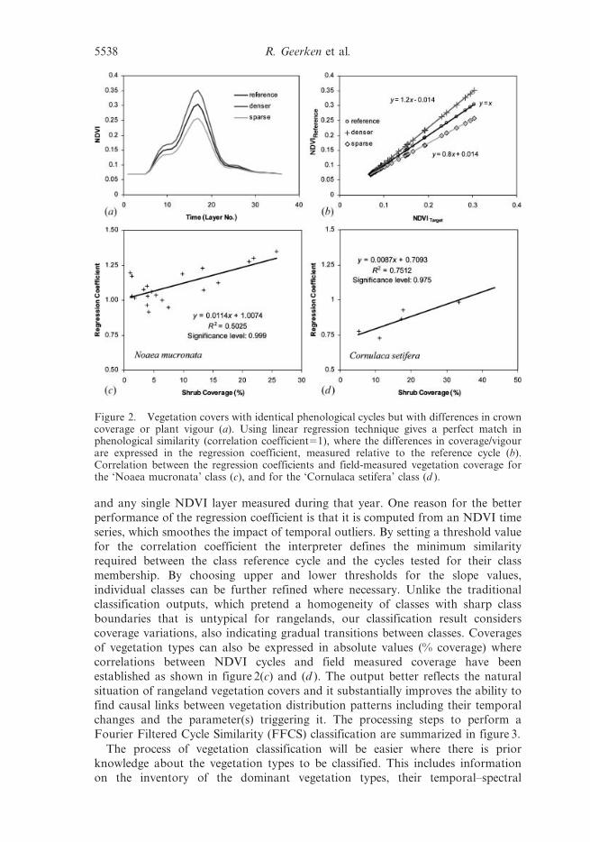
techniques, where the correlation coefficient is the measure for similarity (figure 2(a)

and (b)). Two cycles showing a perfect match in their phenologies have a correlation

coefficient of 1. Phenologies indicating a perfect match may differ in absolute NDVI

values, but this difference will show in the corresponding regression coefficient

(slope value) which can have values greater or smaller than 1. These variations can

be interpreted as variations in vegetation coverage or vegetation vigour (figure 2(b)).

Geerken et al. (2004) show that the regression coefficients are well correlated with

vegetation coverage (figure 2(c) and (d )), providing higher correlation coefficients

and higher levels of significance than those calculated between vegetation coverage

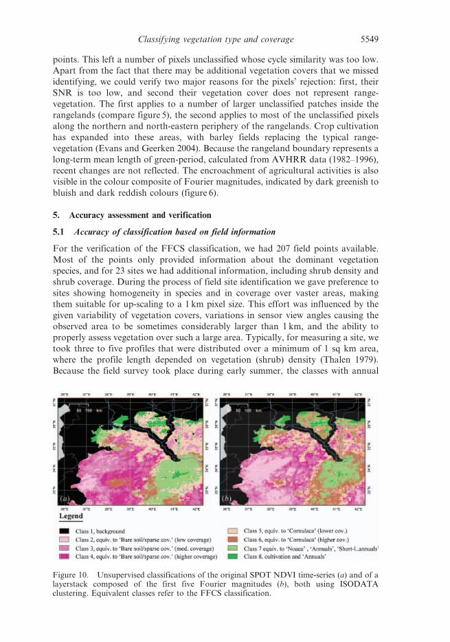
Figure 1. Location map and distribution of sampling points (A.S.5Aleppo Steppe,B.Mt.5Bishri Mountain).

Classifying vegetation type and coverage 5537

and any single NDVI layer measured during that year. One reason for the better

performance of the regression coefficient is that it is computed from an NDVI time

series, which smoothes the impact of temporal outliers. By setting a threshold value

for the correlation coefficient the interpreter defines the minimum similarity

required between the class reference cycle and the cycles tested for their class

membership. By choosing upper and lower thresholds for the slope values,

individual classes can be further refined where necessary. Unlike the traditional

classification outputs, which pretend a homogeneity of classes with sharp class

boundaries that is untypical for rangelands, our classification result considers

coverage variations, also indicating gradual transitions between classes. Coverages

of vegetation types can also be expressed in absolute values (% coverage) where

correlations between NDVI cycles and field measured coverage have been

established as shown in figure 2(c) and (d ). The output better reflects the natural

situation of rangeland vegetation covers and it substantially improves the ability to

find causal links between vegetation distribution patterns including their temporal

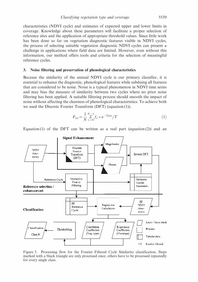
changes and the parameter(s) triggering it. The processing steps to perform a

Fourier Filtered Cycle Similarity (FFCS) classification are summarized in figure 3.

The process of vegetation classification will be easier where there is prior

knowledge about the vegetation types to be classified. This includes information

on the inventory of the dominant vegetation types, their temporal–spectral

Figure 2. Vegetation covers with identical phenological cycles but with differences in crowncoverage or plant vigour (a). Using linear regression technique gives a perfect match inphenological similarity (correlation coefficient51), where the differences in coverage/vigourare expressed in the regression coefficient, measured relative to the reference cycle (b).Correlation between the regression coefficients and field-measured vegetation coverage forthe ‘Noaea mucronata’ class (c), and for the ‘Cornulaca setifera’ class (d ).


characteristics (NDVI cycle) and estimates of expected upper and lower limits in

coverage. Knowledge about these parameters will facilitate a proper selection of

reference sites and the application of appropriate threshold values. Since little work

has been done so far on vegetation diagnostic features visible in NDVI cycles,

the process of selecting suitable vegetation diagnostic NDVI cycles can present a

challenge in applications where field data are limited. However, even without this

information, our method offers tools and criteria for the selection of meaningful

reference cycles.

3. Noise filtering and preservation of phenological characteristics

Because the similarity of the annual NDVI cycle is our primary classifier, it is

essential to enhance the diagnostic, phenological features while subduing all features

that are considered to be noise. Noise is a typical phenomenon in NDVI time series

and may bias the measure of similarity between two cycles where no prior noise

filtering has been applied. A suitable filtering process should smooth the impact of

noise without affecting the clearness of phenological characteristics. To achieve both

we used the Discrete Fourier Transform (DFT) (equation (1)).

F uð Þ~1

NS

N{1

x~0fx � e{2pux=T ð1Þ

Equation (1) of the DFT can be written as a real part (equation (2)) and an

Figure 3. Processing flow for the Fourier Filtered Cycle Similarity classification. Stepsmarked with a black triangle are only processed once; others have to be processed repeatedlyfor every single class.


imaginary part (equation (3)),

FC uð Þ~1

N

XN{1

x~0

f xð Þ � cos 2pux

T

� �� ð2Þ

FS uð Þ~1

N

XN{1

x~0

f xð Þ � sin 2pux

T

� �� ð3Þ

with the Fourier magnitudes (FMagnitudes) calculated as

F Magnitudeð Þu~ffiffiffiffiffiffiffiffiffiffiffiffiffiffiffiffiffiffiffiffiffiffiffiffiffiF2

C uð ÞzF 2S uð Þ

qð4Þ

and the phases (FPhase) as

F Phaseð Þu~atan2FC uð ÞFS uð Þ

� �ð5Þ

The DFT decomposes any complex waveform into sinusoids of different

frequencies or so-called harmonics, which together sum up to the original waveform

(Pavlidis 1982). Once separated into its individual sinusoids, individual frequencies

can be filtered or weighted and summed up thereafter to rebuild a complex

waveform with the noise frequencies being removed. Preceding the classification, we

use this technique to measure and to remove noise from the NDVI layerstack.

Accordingly, we calculated the one-dimensional Fourier parameters in the temporalspace from a 1-year SPOT NDVI layerstack using equations (2) to (5). The highest

frequency resolved in the DFT is the Nyquist frequency that equals half the number

of the samples. The outputs calculated from the 36 SPOT NDVI layers are two 18-

layer data stacks, one containing the 18 Fourier magnitudes and the other the 18

phases. Because SPOT VEGETATION data are not composited at exactly equal

time intervals (periods from 9 to 11 days) we used the NDVI layer number in our

calculation instead of the actual time periods.

3.1 Signal to noise analysis

Statistically most of the variability of annual NDVI cycles is contained in the first

two components. Depending on the intra-annual dynamics of an NDVI cycle,

harmonics one and two account for 50–90% of a cycle’s variability. Discarding all

but the first two components and calculating the inverse Fourier transform to

rebuild the NDVI cycles, creates smooth NDVI cycles while preserving most of the

information, as was demonstrated by Moody and Johnson (2001), who used DFT toassess the productivity of vegetation covers in various climatic environments from

an Advanced Very High Resolution Radiometer (AVHRR) time series. Similarly,

F(Magnitude)u5Fourier magnitude f(x)5is the xth sample value (here: xth NDVI value)FC(u)5cosine (real part) u5number of Fourier component or harmonicFS(u)5sine (imaginary part) x5layer number or Julian Day of NDVI layer (equal

intervals)F(Phase)u5phase

T5length of time period covered; where time ismeasured in number of NDVI layers (T5N )


Andres et al. (1994) used the first two components that were each individually

submitted to a minimum distance classification, with the classification results being

merged thereafter. Olsson and Eklundh (1994) like Azzali and Menenti (2000)concentrated on the first two harmonics to classify mono-modal and bi-modal

vegetation covers. Olsson and Eklundh (1994) used thresholds applied to the

percentage of variance explained in each harmonic for class separation; Azzali and

Menenti used ISODATA classification. Menenti et al. (1993) demonstrate the

usefulness of the first two Fourier components to separate different agroecological

zones, based on differences in amplitude and phase. However, for NDVI cycles from

steppe vegetation covers, discarding all but the first two or three harmonics will

cause unacceptable blurring of the cycles’ diagnostic features. Since our concept fordiscriminating vegetation covers is based on their sometimes subtle phenological

differences, the general application of just the first two harmonics is not practicable.

While we tend to interpret any irregularities that cause deviations from a smooth

NDVI cycle as noise, some of these may actually be realistic NDVI fluctuations.Triggered by growth impulses as induced by sporadic rainfall, and followed by drier

periods, they may be part of a natural plant cycle. Distinguishing noise from rapid

growth can be difficult, especially where temporal spectral field measurements about

a certain species are not available. Any absolute measure of the noise level contained

in an NDVI cycle, therefore, is not possible. Some kind of a proxy-noise measure,

however, is needed to compare the quality of annual NDVI datasets, to assess a

pixel’s suitability as a reference, and to support post-classification analyses such as

explaining why pixels remained unclassified.

As we will demonstrate later, phenology-related information is generally

contained in the first five harmonics. Accordingly, in a scene-wide noise assessment,

we assume that all components higher than five contain only noise, with the total

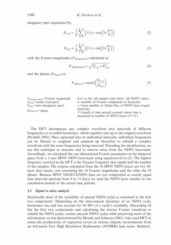
noise being calculated as the sum of harmonics 6–18. For the example of a singleNDVI cycle, the separation of signal from noise through Fourier filtering is shown

in figure 4(a) and (b). To visualize spatial signal to noise ratio (SNR) variations in

the 36 temporal NDVI layers, we tested several approaches. The ratio calculated

between the signal mean and the standard deviation of the noise (equation (6))

proved to be the most appropriate, providing a meaningful SNR assessment for

most NDVI cycles. For a better judgment of how well temporal NDVI features are

resolved, the ratio calculated from the signal range (NDVImax – NDVImin) divided

by the noise standard deviation (equation (7)) may be more appropriate, but it willproduce extremely low SNRs for cycles with low intra-annual dynamics (bare soils,

Figure 4. Original NDVI cycle and after Fourier filtering, showing the cycle’s signalcomponent, and its noise component (a). Weights applied to the individual harmonics toseparate the signal from the noise (b).


very sparsely vegetated).

SNR~MeanNDVISignal

StDevNoise

ð6Þ

or

SNR~MaxNDVISignal{MinNDVISignal

StDevNoise

ð7Þ

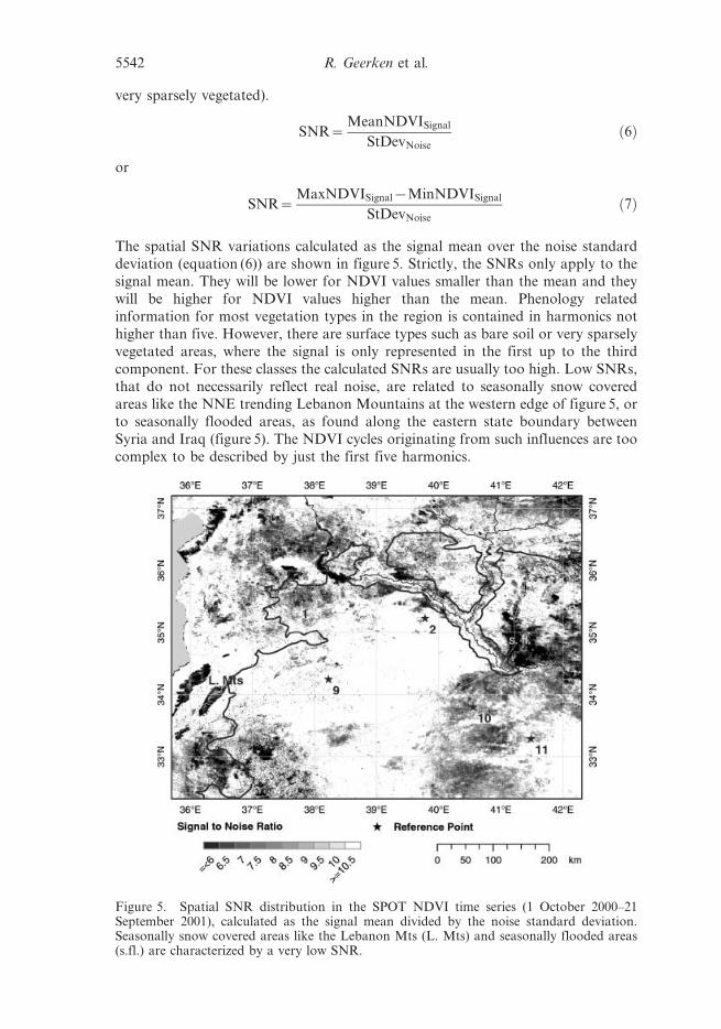
The spatial SNR variations calculated as the signal mean over the noise standard

deviation (equation (6)) are shown in figure 5. Strictly, the SNRs only apply to the

signal mean. They will be lower for NDVI values smaller than the mean and they

will be higher for NDVI values higher than the mean. Phenology related

information for most vegetation types in the region is contained in harmonics not

higher than five. However, there are surface types such as bare soil or very sparsely

vegetated areas, where the signal is only represented in the first up to the third

component. For these classes the calculated SNRs are usually too high. Low SNRs,

that do not necessarily reflect real noise, are related to seasonally snow covered

areas like the NNE trending Lebanon Mountains at the western edge of figure 5, or

to seasonally flooded areas, as found along the eastern state boundary between

Syria and Iraq (figure 5). The NDVI cycles originating from such influences are too

complex to be described by just the first five harmonics.

Figure 5. Spatial SNR distribution in the SPOT NDVI time series (1 October 2000–21September 2001), calculated as the signal mean divided by the noise standard deviation.Seasonally snow covered areas like the Lebanon Mts (L. Mts) and seasonally flooded areas(s.fl.) are characterized by a very low SNR.


Because the clearness of a distinct diagnostic feature in the NDVI cycle variesdepending on the vegetation type’s coverage or its mixture with other vegetation

types, it is impossible to define a fixed SNR suitable for the identification of any

phenological feature. Considering the given land cover characteristics of the Syrian

Steppe and the technical limits encountered in detecting features from some

vegetation types at very low coverage, we limited our analysis to vegetation types

whose coverages range from 30% or higher down to 5–10%. The 5% coverage

threshold was concluded from a study (Geerken et al. 2004) that related field-

measured vegetation coverages with the slope values calculated between thereference cycle and the sites’ target cycles (figure 2(a) and (c)). The correlation

between the regression coefficients and the field-measured vegetation coverages got

increasingly worse, when coverages below 10% were included. Below 5%, the

scattergrams showed such high variance that a reliable coverage assessment in this

range was deemed to be unrealistic. A possible reason may be the inadequate size,

especially of some of the more sparsely vegetated measuring sites, for upscaling to a

SPOT pixel size that varies temporally with view angle. The SPOT pixel size,

considering all measuring sites over the one-year time period, ranges between 1170–4650 m with a calculated mean of 2635 m. An acceptable minimum SNR, required to

detect the phenological features of interest, is at around 8 : 1. However, a lower SNR

does not necessarily prevent a cycle from being properly identified. As we will show

later, the calculated SNR is merely an indicator for a possible noise effect; it does

not necessarily reflect the actual noise contained in a signal.

3.2 Selection of reference NDVI cycles

The map with the spatial SNR distribution (figure 5) is a valuable source of

information during the selection process of reference cycles. Excluding cycles that

are likely to have a low SNR as reference sites will considerably improve

classification results. Following the classification, the SNR map can help analyse

whether unclassified pixels represent an additional vegetation type that had been

missed or whether they remained unclassified because of their low SNR. The

selection of reference sites for this classification is based on field information and on

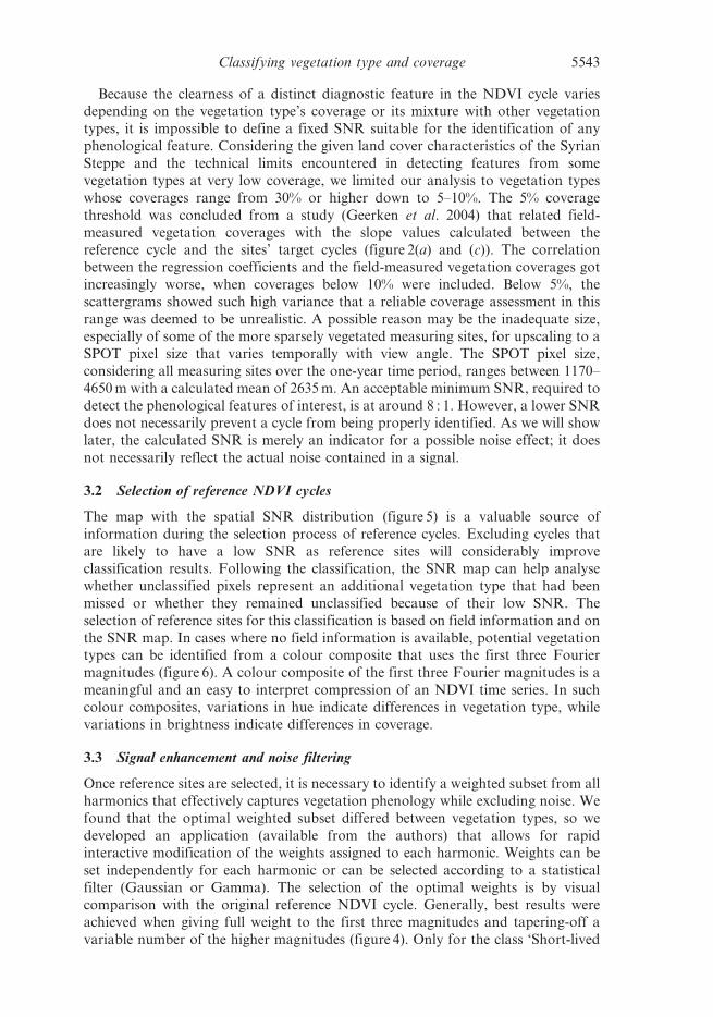
the SNR map. In cases where no field information is available, potential vegetationtypes can be identified from a colour composite that uses the first three Fourier

magnitudes (figure 6). A colour composite of the first three Fourier magnitudes is a

meaningful and an easy to interpret compression of an NDVI time series. In such

colour composites, variations in hue indicate differences in vegetation type, while

variations in brightness indicate differences in coverage.

3.3 Signal enhancement and noise filtering

Once reference sites are selected, it is necessary to identify a weighted subset from all

harmonics that effectively captures vegetation phenology while excluding noise. We

found that the optimal weighted subset differed between vegetation types, so we

developed an application (available from the authors) that allows for rapid

interactive modification of the weights assigned to each harmonic. Weights can be

set independently for each harmonic or can be selected according to a statistical

filter (Gaussian or Gamma). The selection of the optimal weights is by visual

comparison with the original reference NDVI cycle. Generally, best results wereachieved when giving full weight to the first three magnitudes and tapering-off a

variable number of the higher magnitudes (figure 4). Only for the class ‘Short-lived


grasses’ we used eight harmonics. Sparsely vegetated areas and bare soil/rock

surfaces, showing only little intra-annual dynamics, are best described by just the

first harmonic. The interactive manipulation of the reference cycles also enables the

smoothing of local impacts on NDVI values, as caused for example by local rainfall

events. The maximum number of harmonics needed to describe a species’ phenology

(NDVI cycle) defines the minimum temporal data resolution required. In our study,

a maximum of eight harmonics used for the enhancement of the ‘Short-lived grass’

class means 16 intervals a year, resulting in a sampling interval of at least every 23

days. Depending on the phenological characteristics of individual species, however,

a higher temporal resolution may be needed.

The weights found optimum for the class reference cycle were then applied to the

entire scene to calculate the inverse Fourier transform and to build a layerstack

optimized for this specific class. The NDVI cycles in the new layerstack are reduced

in noise and enhanced for this class’s phenological characteristics. Because of spatial

SNR variations, the application of the parameters as they were found optimum for

the reference-cycle will provide variable results for pixels with a different noise

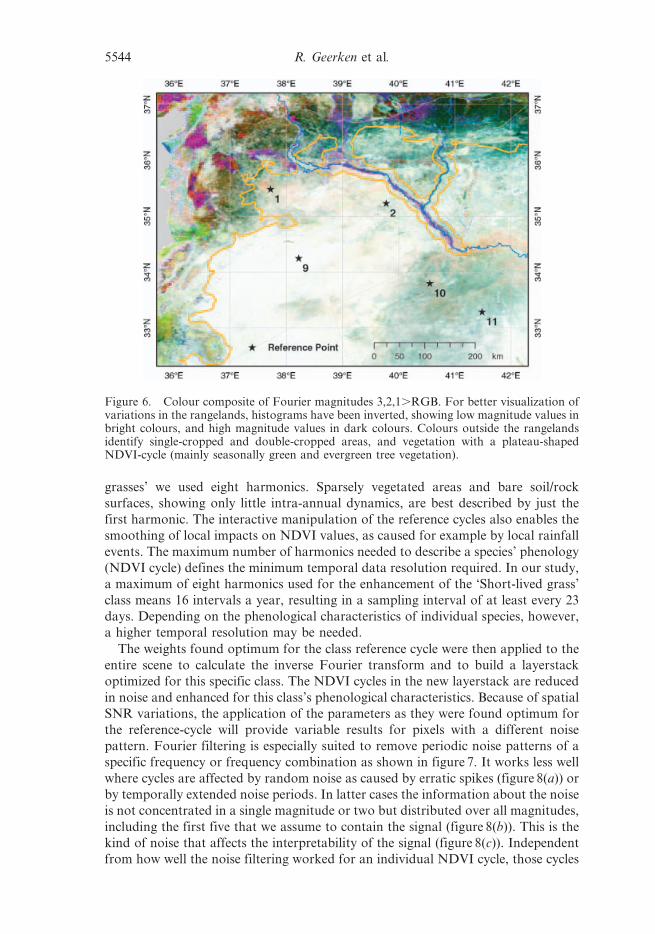
pattern. Fourier filtering is especially suited to remove periodic noise patterns of a

specific frequency or frequency combination as shown in figure 7. It works less well

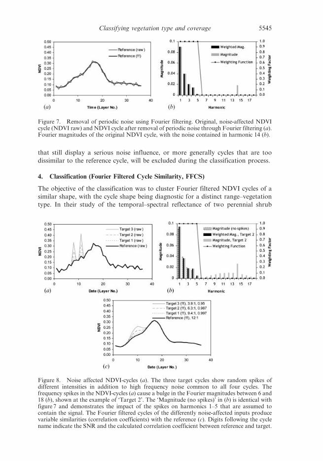
where cycles are affected by random noise as caused by erratic spikes (figure 8(a)) or

by temporally extended noise periods. In latter cases the information about the noise

is not concentrated in a single magnitude or two but distributed over all magnitudes,

including the first five that we assume to contain the signal (figure 8(b)). This is the

kind of noise that affects the interpretability of the signal (figure 8(c)). Independent

from how well the noise filtering worked for an individual NDVI cycle, those cycles

Figure 6. Colour composite of Fourier magnitudes 3,2,1.RGB. For better visualization ofvariations in the rangelands, histograms have been inverted, showing low magnitude values inbright colours, and high magnitude values in dark colours. Colours outside the rangelandsidentify single-cropped and double-cropped areas, and vegetation with a plateau-shapedNDVI-cycle (mainly seasonally green and evergreen tree vegetation).


that still display a serious noise influence, or more generally cycles that are too

dissimilar to the reference cycle, will be excluded during the classification process.

4. Classification (Fourier Filtered Cycle Similarity, FFCS)

The objective of the classification was to cluster Fourier filtered NDVI cycles of a

similar shape, with the cycle shape being diagnostic for a distinct range–vegetation

type. In their study of the temporal–spectral reflectance of two perennial shrub

Figure 7. Removal of periodic noise using Fourier filtering. Original, noise-affected NDVIcycle (NDVI raw) and NDVI cycle after removal of periodic noise through Fourier filtering (a).Fourier magnitudes of the original NDVI cycle, with the noise contained in harmonic 14 (b).

Figure 8. Noise affected NDVI-cycles (a). The three target cycles show random spikes ofdifferent intensities in addition to high frequency noise common to all four cycles. Thefrequency spikes in the NDVI-cycles (a) cause a bulge in the Fourier magnitudes between 6 and18 (b), shown at the example of ‘Target 2’. The ‘Magnitude (no spikes)’ in (b) is identical withfigure 7 and demonstrates the impact of the spikes on harmonics 1–5 that are assumed tocontain the signal. The Fourier filtered cycles of the differently noise-affected inputs producevariable similarities (correlation coefficients) with the reference (c). Digits following the cyclename indicate the SNR and the calculated correlation coefficient between reference and target.


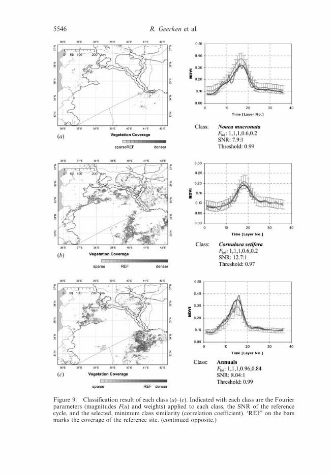
Figure 9. Classification result of each class (a)–(e). Indicated with each class are the Fourierparameters (magnitudes F(u) and weights) applied to each class, the SNR of the referencecycle, and the selected, minimum class similarity (correlation coefficient). ‘REF’ on the barsmarks the coverage of the reference site. (continued opposite.)


species and of annual grasses, Geerken et al. (2004) identified characteristic

differences in the species’ spectral cycles. The degraded shrub species Noaea

mucronata is characterized by an extended growing period (Rae et al. 2001),

triggering NDVI values that are considerably higher during the dry season than

those measured for the annual grasses and for the non-degraded shrub species

Artemisia herba alba. A differentiation between the latter two based on their NDVI

cycles is not possible. Another widespread degraded species is Cornulaca setifera.

Though no temporal–spectral field measurements have been done to study its

temporal–spectral characteristics, the image cycles of verified field locations indicate

an even more pronounced extended growing period for this species. Depending on

the location either of the degraded species is dominant in vegetation covers of the

Syrian Steppe. Artemisia herba alba only occurs in small, scattered, and often

protected plots. With regard to the limited information that is currently available

about the differentiability of species based on their NDVI cycles, it was our aim to

classify vegetation covers that are dominated by either of the following species:

Noaea mucronata, Cornulaca setifera or annual grasses (figure 9(a), (b) and (c)). In

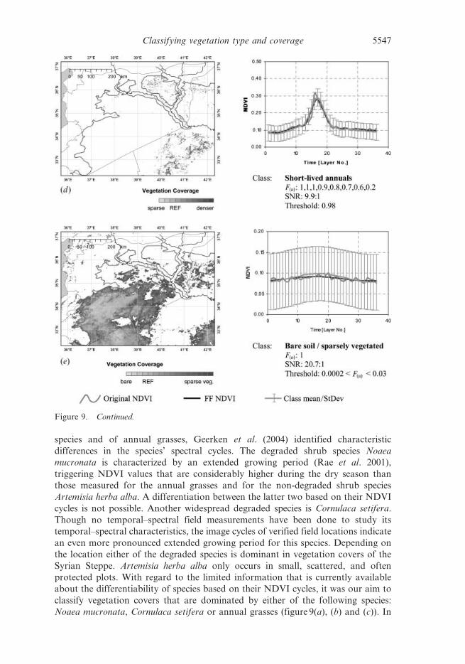
Figure 9. Continued.


addition to that it was the aim to further separate the very sparsely covered (annual

grasses) to bare soil areas (figure 9(e)). After a first classification run we identified

another vegetation type, represented by the ‘Short-lived annuals’ class (figure 9(d )),

which we have not had the possibility to verify in the field. It is characterized by a

very short green-period.

A suitable algorithm that measures the similarity between NDVI cycles was

required to be invariant to changes in cycle amplitude, as caused by plant coverage

or plant vigour, and to be invariant to translational shifts in the temporal domain,

as may occur in areas with a strong climate gradient. These translational shifts are

not purely translational when looking into a limited time period like one year. By

shifting the NDVI cycle, NDVI values move out at one end of the time period, while

others move in at the other end of the time period. Typical shape similarity

algorithms, as discussed by Loncaric (1998), tend to focus on invariance to rotation

and to scale, which are fixed parameters in our case. The definition of invariance to

translational shifts in such algorithms is different from the definition relevant to a

cyclic phenology and cannot be applied to the signatures we intended to classify.

As a simple solution, we used linear correlation techniques, where the Fourier

filtered reference NDVI cycle is correlated with the likewise Fourier filtered NDVI

layerstack. The calculated correlation coefficient is our measure for cycle similarity.

It is invariant to the cycle amplitude (figure 2(a) and (b)) but sensitive to

phenological changes. Among the phenological differences, we were especially

interested in variations that can be related to distinct vegetation types. To separate

these from variations that merely represent a temporal shift of the same vegetation

type across a climate gradient, the reference cycle was cycled through the NDVI

layerstack. This was achieved by a stepwise, temporal shifting of the reference, with

the NDVI values that move out at one end of the time period being cycled in at the

other end of the time period. The correlation coefficient was calculated for each

time-step, with the maximum correlation defining a cycle’s similarity with the

reference. The corresponding regression coefficients are a measure of the percentage

coverage relative to the reference. By thresholding the layer of maximum correlation

coefficients, the interpreter defines the minimum similarity required for a specific

class. Admission of a pixel to a specific class can then be further constraint on the

basis of percentage coverage, by setting upper and lower limits for the regression

coefficient. The result is a classification that shows the distribution of a class’s

dominant vegetation type, including its spatial variations in coverage (figure 9). This

process, starting with the definition of optimum Fourier parameters for the

reference cycle, followed by the similarity measure and thresholding, must be

repeated for each class (figure 3).

As expected, there is some overlap between classes, especially along their

peripheries, suggesting gradual transitions between cover types. This is also

expressed by decreasing coverages towards the periphery of at least one class

(figure 9). As a technical solution, a pixel is allocated to the class with which it is

most strongly correlated. In a case of equal correlation coefficients, the higher total

of Fourier weights is decisive. Because we were not able to sample all classes in the

field in order to establish correlations between %vegetation coverage and regression

coefficient (figure 2(c) and (d )), vegetation coverage for all classes is only given

relative to the reference cycle (figures 9 and 10).

When setting the thresholds for similarity and coverage, it was the primary

objective to achieve the maximum agreement between the classification and our field


points. This left a number of pixels unclassified whose cycle similarity was too low.

Apart from the fact that there may be additional vegetation covers that we missed

identifying, we could verify two major reasons for the pixels’ rejection: first, their

SNR is too low, and second their vegetation cover does not represent range-

vegetation. The first applies to a number of larger unclassified patches inside the

rangelands (compare figure 5), the second applies to most of the unclassified pixels

along the northern and north-eastern periphery of the rangelands. Crop cultivation

has expanded into these areas, with barley fields replacing the typical range-

vegetation (Evans and Geerken 2004). Because the rangeland boundary represents a

long-term mean length of green-period, calculated from AVHRR data (1982–1996),

recent changes are not reflected. The encroachment of agricultural activities is also

visible in the colour composite of Fourier magnitudes, indicated by dark greenish to

bluish and dark reddish colours (figure 6).

5. Accuracy assessment and verification

5.1 Accuracy of classification based on field information

For the verification of the FFCS classification, we had 207 field points available.

Most of the points only provided information about the dominant vegetation

species, and for 23 sites we had additional information, including shrub density and

shrub coverage. During the process of field site identification we gave preference to

sites showing homogeneity in species and in coverage over vaster areas, making

them suitable for up-scaling to a 1 km pixel size. This effort was influenced by the

given variability of vegetation covers, variations in sensor view angles causing the

observed area to be sometimes considerably larger than 1 km, and the ability to

properly assess vegetation over such a large area. Typically, for measuring a site, we

took three to five profiles that were distributed over a minimum of 1 sq km area,

where the profile length depended on vegetation (shrub) density (Thalen 1979).

Because the field survey took place during early summer, the classes with annual

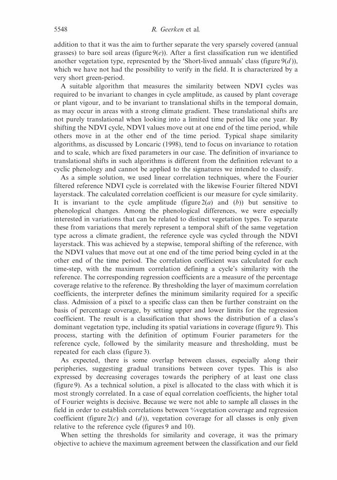
Figure 10. Unsupervised classifications of the original SPOT NDVI time-series (a) and of alayerstack composed of the first five Fourier magnitudes (b), both using ISODATAclustering. Equivalent classes refer to the FFCS classification.


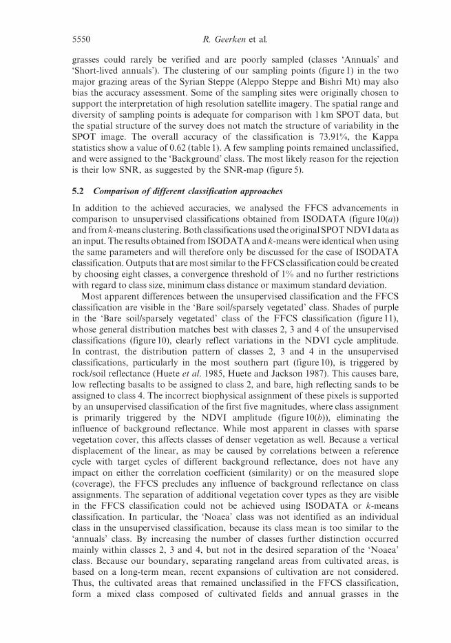
grasses could rarely be verified and are poorly sampled (classes ‘Annuals’ and

‘Short-lived annuals’). The clustering of our sampling points (figure 1) in the two

major grazing areas of the Syrian Steppe (Aleppo Steppe and Bishri Mt) may also

bias the accuracy assessment. Some of the sampling sites were originally chosen to

support the interpretation of high resolution satellite imagery. The spatial range and

diversity of sampling points is adequate for comparison with 1 km SPOT data, but

the spatial structure of the survey does not match the structure of variability in the

SPOT image. The overall accuracy of the classification is 73.91%, the Kappa

statistics show a value of 0.62 (table 1). A few sampling points remained unclassified,

and were assigned to the ‘Background’ class. The most likely reason for the rejection

is their low SNR, as suggested by the SNR-map (figure 5).

5.2 Comparison of different classification approaches

In addition to the achieved accuracies, we analysed the FFCS advancements in

comparison to unsupervised classifications obtained from ISODATA (figure 10(a))

and from k-means clustering. Both classifications used the original SPOT NDVI data as

an input. The results obtained from ISODATA and k-means were identical when using

the same parameters and will therefore only be discussed for the case of ISODATA

classification. Outputs that are most similar to the FFCS classification could be created

by choosing eight classes, a convergence threshold of 1% and no further restrictions

with regard to class size, minimum class distance or maximum standard deviation.

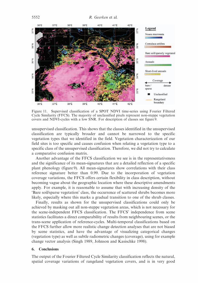
Most apparent differences between the unsupervised classification and the FFCS

classification are visible in the ‘Bare soil/sparsely vegetated’ class. Shades of purple

in the ‘Bare soil/sparsely vegetated’ class of the FFCS classification (figure 11),

whose general distribution matches best with classes 2, 3 and 4 of the unsupervised

classifications (figure 10), clearly reflect variations in the NDVI cycle amplitude.

In contrast, the distribution pattern of classes 2, 3 and 4 in the unsupervised

classifications, particularly in the most southern part (figure 10), is triggered by

rock/soil reflectance (Huete et al. 1985, Huete and Jackson 1987). This causes bare,

low reflecting basalts to be assigned to class 2, and bare, high reflecting sands to be

assigned to class 4. The incorrect biophysical assignment of these pixels is supported

by an unsupervised classification of the first five magnitudes, where class assignment

is primarily triggered by the NDVI amplitude (figure 10(b)), eliminating the

influence of background reflectance. While most apparent in classes with sparse

vegetation cover, this affects classes of denser vegetation as well. Because a vertical

displacement of the linear, as may be caused by correlations between a reference

cycle with target cycles of different background reflectance, does not have any

impact on either the correlation coefficient (similarity) or on the measured slope

(coverage), the FFCS precludes any influence of background reflectance on class

assignments. The separation of additional vegetation cover types as they are visible

in the FFCS classification could not be achieved using ISODATA or k-means

classification. In particular, the ‘Noaea’ class was not identified as an individual

class in the unsupervised classification, because its class mean is too similar to the

‘annuals’ class. By increasing the number of classes further distinction occurred

mainly within classes 2, 3 and 4, but not in the desired separation of the ‘Noaea’

class. Because our boundary, separating rangeland areas from cultivated areas, is

based on a long-term mean, recent expansions of cultivation are not considered.

Thus, the cultivated areas that remained unclassified in the FFCS classification,

form a mixed class composed of cultivated fields and annual grasses in the


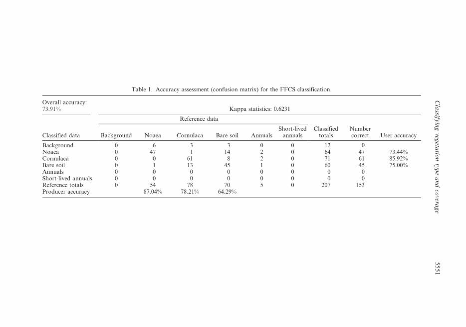
Table 1. Accuracy assessment (confusion matrix) for the FFCS classification.

Overall accuracy:73.91% Kappa statistics: 0.6231

Classified data

Reference data

Classifiedtotals

Numbercorrect User accuracyBackground Noaea Cornulaca Bare soil Annuals

Short-livedannuals

Background 0 6 3 3 0 0 12 0Noaea 0 47 1 14 2 0 64 47 73.44%Cornulaca 0 0 61 8 2 0 71 61 85.92%Bare soil 0 1 13 45 1 0 60 45 75.00%Annuals 0 0 0 0 0 0 0 0Short-lived annuals 0 0 0 0 0 0 0 0Reference totals 0 54 78 70 5 0 207 153Producer accuracy 87.04% 78.21% 64.29%

Cla

ssifyin

gveg

etatio

nty

pe

an

dco

verag

e5

55

1

unsupervised classification. This shows that the classes identified in the unsupervised

classification are typically broader and cannot be narrowed to the specific

vegetation types that we identified in the field. Vegetation characterization of our

field sites is too specific and causes confusion when relating a vegetation type to a

specific class of the unsupervised classification. Therefore, we did not try to calculate

a comparative confusion matrix.

Another advantage of the FFCS classification we see is in the representativeness

and the significance of its mean-signatures that are a detailed reflection of a specific

plant phenology (figure 9). All mean-signatures show correlations with their class

reference signature better than 0.99. Due to the incorporation of vegetation

coverage variations, the FFCS offers certain flexibility in class description, without

becoming vague about the geographic location where these descriptive amendments

apply. For example, it is reasonable to assume that with increasing density of the

‘Bare soil/sparse vegetation’ class, the occurrence of scattered shrubs becomes more

likely, especially where this marks a gradual transition to one of the shrub classes.

Finally, results as shown for the unsupervised classifications could only be

achieved by masking out all non-steppe vegetation areas, which is not necessary for

the scene-independent FFCS classification. The FFCS’ independence from scene

statistics facilitates a direct comparability of results from neighbouring scenes, or the

trans-scene application of reference-cycles. Multi-temporal classifications based on

the FFCS further allow more realistic change detection analyses that are not biased

by scene statistics, and have the advantage of visualizing categorical changes

(vegetation type) as well as subtle radiometric changes (coverage), using for example

change vector analysis (Singh 1989, Johnson and Kasischke 1998).

6. Conclusions

The output of the Fourier Filtered Cycle Similarity classification reflects the natural,

spatial coverage variations of rangeland vegetation covers, and is in very good

Figure 11. Supervised classification of a SPOT NDVI time-series using Fourier FilteredCycle Similarity (FFCS). The majority of unclassified pixels represent non-steppe vegetationcovers and NDVI-cycles with a low SNR. For description of classes see figure 9.


agreement with field data. The five classes, ‘Noaea’, ‘Cornulaca’, ‘Annuals’, ‘Short-

lived annuals’, and ‘Bare soil/sparsely vegetated’, outline the dominant vegetation

covers including their intra-class coverage variations in a meaningful way. Using

field data for the assessments of the Noaea class, the Cornulaca class, and of the

Bare soil/sparsely vegetated class resulted in accuracies between 64% and 87% (user

and producer accuracy). Besides the improvements in capturing spatial distribution

and variability of dominant species, we consider the possibility of a more diagnostic

description of classes in terms of their ecological value as particularly important.

These advances in vegetation classification we ascribe to the technique’s emphasis

on shape classification and to the consideration of typical dryland vegetation

features, such as coverage variation, climate induced phenological shifts, and

background influences. The interpreter’s full control over all classification

parameters at all times, including the setting of the required similarity for each

individual class, is another factor ensuring accurate and meaningful results. A major

shortcoming may be the considerable computation time needed for the DFT, the

inverse DFT, the similarity measure, and the interactive thresholding. However,

considering the time needed in unsupervised classifications, to carefully mask out

non-steppe vegetation and areas with cloud cover and cloud shadows (Peters et al.

1997), the difference may not be very significant. While we do not consider the

presence of unclassified areas as a weakness of the technique, especially not where

data noise is the reason, it is of course desirable to fill in the missing information. A

solution to that could be the compositing of classification outputs from different

years. Where these do not differ too much in time, relative changes between the

reference site and the targets should be negligible. Currently, our knowledge about

NDVI vegetation cycles, their linkage to vegetation type, and the characteristics of

the phenological cycle they reflect, is very limited. Therefore, to successfully apply

the FFCS classification, the interpretation of NDVI cycles, their biophysical

meaning and their differentiability, requires further studying. The FFCS classifica-

tion relies on information contained in NDVI cycle variability, and its applicability

will benefit from further study of the biophysics and ecology that drive this

variability.

By providing detailed information about vegetation covers, describing vegetation

type and mapping vegetation coverage, the classification holds great potential not

only for rangeland management, but also for a better assessment of the rangelands’

importance in carbon sequestration, or for modelling landscape scale hydrological

processes.

Acknowledgments

This study was carried out as part of the research project ‘Environmental Changes in

the Near East’ (NAG5-9316) supported and financed by NASA’s Interdisciplinary

Science Program as well as ‘The Water Cycle of the Tigris–Euphrates Watershed:

Natural Processes and Human Impacts’ (NNG05GB36G). The authors wish to

thank Ron Smith for his contributions to this study during discussions. We also

want to thank people at the International Center for Agricultural Research in

the Dry Areas (ICARDA) in Aleppo, who contributed to this study through

their logistic support during field surveys and through their expertise in Syrian

rangeland vegetation covers. We further want to extend our thanks to the SPOT

VEGETATION production and distribution team for making available the data

used in this study.


ReferencesAGUIAR, M.R., PARUELO, J.M., SALA, O.E. and LAUENROTH, W.K., 1996, Ecosystem

responses to changes in plant functional type composition: an example from the

Patagonian steppe. Journal of Vegetation Science, 7, pp. 381–390.

ANDRES, L., SALS, W.A. and SKOLE, D., 1994, Fourier-analysis of multitemporal AVHRR-

data applied to a land-cover classification. International Journal of Remote Sensing,

15, pp. 1115–1121.

AZZALI, S. and MENENTI, M., 2000, Mapping vegetation–soil–climate complexes in southern

Africa using temporal Fourier analysis of NOAA-AVHRR data. International

Journal of Remote Sensing, 21, pp. 973–996.

EVANS, J. and GEERKEN, R., 2004, Discrimination between climate and human induced

dryland degradation. Journal of Arid Environments, 57, pp. 535–554.

GEERKEN, R., BATHIKA, N., CELIS, D. and DEPAUW, E., 2004, Differentiation of rangeland

vegetation—hyperspectral field investigations and MODIS and SPOT data analyses.

International Journal of Remote Sensing (in press).

HOLMES, T.H. and RICE, K.J., 1996, Patterns of growth and soil-water utilization in some

exotic annuals and native perennial bunchgrasses of California. Annals of Botany,

78(2), pp. 233–243.

HUETE, A.R. and JACKSON, R.D., 1987, Suitability of spectral indices for evaluating vegetation

characteristics on arid rangelands. Remote Sensing of Environment, 23, pp. 213–232.

HUETE, A.R., JACKSON, R.D. and POST, D.F., 1985, Spectral response of plant canopy with

different soil backgrounds. Remote Sensing of Environment, 17, pp. 37–53.

JOHNSON, R.D. and KASISCHKE, E.S., 1998, Change vector analysis: a technique for the

multispectral monitoring of land cover condition. International Journal of Remote

Sensing, 19, pp. 411–426.

LeHouerou, H.N., 1996, Climate change, drought and desertification. Journal of Arid

Environments, 34, pp. 133–185.

LONCARIC, S.,1998, A surveyof shape analysis techniques.PatternRecognition, 31, pp.983–1001.

MENENTI, M., AZZALI, S., VERHOEF, W. and VAN SWOL, R., 1993, Mapping agroecological

zones and time-lag in vegetation growth by means of Fourier analysis of time series of

NDVI images. Advances in Space Research, 13(5), pp. 233–237.

MOODY, A. and JOHNSON, D.M., 2001, Land-surface phenologies from AVHRR using the

discrete fourier transform. Remote Sensing of Environment, 75, pp. 305–323.

OLSSON, L. and EKLUNDH, L., 1994, Fourier-series for analysis of temporal sequences of

satellite sensor imagery. International Journal of Remote Sensing, 15, pp. 3735–3741.

PAVLIDIS, T., 1982, Algorithms for Graphics and Image Processing (Rockville, MD: Computer

Science Press).

PETERS, A.J., EVE, M.D., HOLT, E.H. and WHITFORD, W.G., 1997, Analysis of desert plant

community growth patterns with high temporal resolution satellite spectra. Journal of

Applied Ecology, 34, pp. 418–432.

RAE, J., ARAB, G., NORDBLOM, T., JANI, K. and GINTZBURGER, G., 2001, Tribes state and

technology adoption in arid land management, Syria. CGIAR Systemwide Program

on Collective Action and Property Rights, CAPRi Working Paper No. 15, IFPRI,

Washington, USA.

SINGH, A., 1989, Digital change detection techniques using remotely sensed data.

International Journal of Remote Sensing, 10, pp. 989–1003.

SPOT VEGETATION 2004, User-Guide, http://www.spot-vegetation.com/vegetationpro-

gramme/Pages/TheVegetationSystem/userguide/userguide.htm.

THALEN, P., 1979, Ecology and utilization of desert shrub rangelands in Iraq. PhD thesis,

Rijksuniversiteit Groningen, The Netherlands (The Hague: Dr W Junk BV).

TOU, J.T. and GONZALEZ, R.C., 1974, Pattern Recognition Principles (Reading, MA:

Addison-Wesley).

5554 Classifying vegetation type and coverage

Documents

Classifying rangeland vegetation type and coverage from NDVI time