Classifying and Comparing Design Optimization Problems

ISR develops, applies and teaches advanced methodologies of design and analysis to solve complex, hierarchical,heterogeneous and dynamic problems of engineering technology and systems for industry and government.

ISR is a permanent institute of the University of Maryland, within the Glenn L. Martin Institute of Technol-ogy/A. James Clark School of Engineering. It is a National Science Foundation Engineering Research Center.

Web site http://www.isr.umd.edu

I RINSTITUTE FOR SYSTEMS RESEARCH

MASTER'S THESIS

Classifying and Comparing Design Optimization Problems

by Brad M. BrochtrupAdvisor:

MS 2006-2

ABSTRACT

Title of Thesis: CLASSIFYING AND COMPARING DESIGN OPTIMIZATION PROBLEMS

Brad Michael Brochtrup, Master of Science, 2006

Thesis directed by: Associate Professor Jeffrey W. Herrmann Department of Mechanical Engineering and Institute for Systems Research

Research in product design optimization has developed and demonstrated a

variety of modeling techniques and solution methods, including multidisciplinary design

optimization. As new techniques migrate to the industrial world engineers are faced with

much more complex problems often extending beyond their realm of knowledge. A

novel classification scheme is proposed and demonstrated to offer engineers a method of

organizing and searching for relevant example problems to assist in the production of

their own optimization problem. To explore the tradeoff between information

requirements and solution quality, computational experiments are conducted on two

design problems, a bathroom scale and a universal electric motor. In particular, the

results of these experiments identify the additional information required to solve a profit

maximization problem, demonstrate the role of rules of thumb in formulating design

optimization problems, show how decomposition affects solution quality and

computational effort, and uncover the impact of using target matching in the objective

function instead of as constraints. In addition, the results show how the values of targets

and objective function weights impact solution quality. In general, these results show the

extent to which correct information is critical to finding a high quality solution, perhaps

more critical than the optimization model selected. That is, the quality of the information

used is more important than the amount of information used.

CLASSIFYING AND COMPARING DESIGN OPTIMIZATION PROBLEMS

by

Brad Michael Brochtrup

Thesis submitted to the Faculty of the Graduate School of the University of Maryland, College Park in partial fulfillment

of the requirements for the degree of Master of Science

2006

Advisory Committee:

Professor Jeffrey W. Herrmann, Chair Professor Shapour Azarm Professor Linda Schmidt

© Copyright by Brad Michael Brochtrup

2006

ii

Acknowledgements

I would like to thank Dr. Jeffrey Herrmann for his continual support throughout

this research. Without his patience, perseverance and guidance my understanding of the

subject matter would not compare.

iii

TABLE OF CONTENTS

LIST OF TABLES .......................................................................................................... IV

LIST OF FIGURES ......................................................................................................... V

LIST OF ACRONYMS ................................................................................................... V

CHAPTER 1: INTRODUCTION................................................................................... 1

CHAPTER 2: BACKGROUND ..................................................................................... 5

CHAPTER 3: METHODOLOGY.................................................................................. 8

3.1 CLASSIFICATION SCHEME .......................................................................................... 8 3.2 COMPUTATIONAL EXPERIMENTS................................................................................ 9

CHAPTER 4: A CLASSIFICATION FRAMEWORK.............................................. 11

4.1 DEFINITIONS ............................................................................................................ 12 4.2 CLASSIFICATION FRAMEWORK................................................................................. 17 4.3 EXAMPLES................................................................................................................ 21

CHAPTER 5: ANALYSIS OF A BATHROOM SCALE .......................................... 27

5.1 ORIGINAL MODEL FORMULATION............................................................................ 28 5.2 OPTIMIZATION SETUPS............................................................................................. 32 5.3 RESULTS OF BATHROOM SCALE ANALYSIS.............................................................. 44 5.4 COMPARING INFORMATION REQUIREMENTS ............................................................ 49 5.5 EFFECTS OF DECOMPOSITION................................................................................... 52

CHAPTER 6: ANALYSIS OF AN ELECTRIC MOTOR......................................... 56

6.1 ORIGINAL MODEL FORMULATION............................................................................ 57 6.2 OPTIMIZATION SETUPS............................................................................................. 61 6.3 RESULTS OF UNIVERSAL ELECTRIC MOTOR ANALYSIS............................................ 67 6.4 COMPARING INFORMATION REQUIREMENTS ............................................................ 72 6.5 USING RULES OF THUMB IN CHOOSING AN OBJECTIVE FUNCTION........................... 75 6.6 TARGET MATCHING IN THE OBJECTIVE.................................................................... 76

CHAPTER 7: DISCUSSION ........................................................................................ 83

CHAPTER 8: SUMMARY AND CONCLUSIONS ................................................... 89

8.1 DESIGN OPTIMIZATION CLASSIFICATION ................................................................. 89 8.2 DESIGN OPTIMIZATION COMPARISON ...................................................................... 90 8.3 FUTURE WORK......................................................................................................... 92

APPENDIX A.................................................................................................................. 94

APPENDIX B .................................................................................................................. 95

REFERENCES................................................................................................................ 97

iv

List of Tables

Table 1: Combinations of Single Product Optimization with a Single Objective. ........... 18 Table 2: Combinations of Single Product Optimization with Multiple Objectives.......... 20 Table 3: Classified Examples from Literature. ................................................................. 26 Table 4: Relation Matrix for Bathroom Scale................................................................... 29 Table 5: Bounds on Product Attributes............................................................................. 31 Table 6: Breakdown of Seven Scale Setups. .................................................................... 34 Table 7: Seven Initial Solutions Used in All Seven Setups. ............................................. 35 Table 8: Target Settings Used in Setup 1.......................................................................... 36 Table 9: Relation Matrix for Setup 2. ............................................................................... 37 Table 10: Relation Matrix for Setup 3. ............................................................................. 38 Table 11: Relation Matrix for Setup 4. ............................................................................. 40 Table 12: Relation Matrix for Setup 5. ............................................................................. 41 Table 13: Relation Matrix for Setup 6. ............................................................................. 42 Table 14: Target Matching Results from Setup 1. ............................................................ 45 Table 15: Weighting Coefficient Analysis Results........................................................... 48 Table 16: Results of Seven Scale Optimization Setups. ................................................... 54 Table 17: Comparing Computational Effort of Scale Analysis. ....................................... 55 Table 18: Relation Matrix for the Universal Electric Motor. ........................................... 57 Table 19: Bounds on Design Variables. ........................................................................... 59 Table 20: Details of the Six Motor Setups........................................................................ 62 Table 21: Initial solutions for Universal Electric Motor Optimizations. .......................... 63 Table 22: Benchmark Motor Designs [37]. ...................................................................... 64 Table 23: Results of Multi-Objective Optimization. ........................................................ 68 Table 24: Results of MO Optimization with Target Settings. .......................................... 69Table 25: Results of Single Objective Optimization to Minimize Mass. ......................... 69 Table 26: Results of Single Objective Optimization to Maximize Efficiency. ................ 70 Table 27: Results of AAO Optimization .......................................................................... 71 Table 28: Comparison of Five Setups on Motor Design 1 ............................................... 78Table 29: Comparison of Five Setups on Motor Design 2 ............................................... 79Table 30: Comparison of Five Setups on Motor Design 3 ............................................... 80Table 31: Comparison of Five Setups on Motor Design 4 ............................................... 81Table 32: Comparison of Five Setups on Motor Design 5 ............................................... 82

v

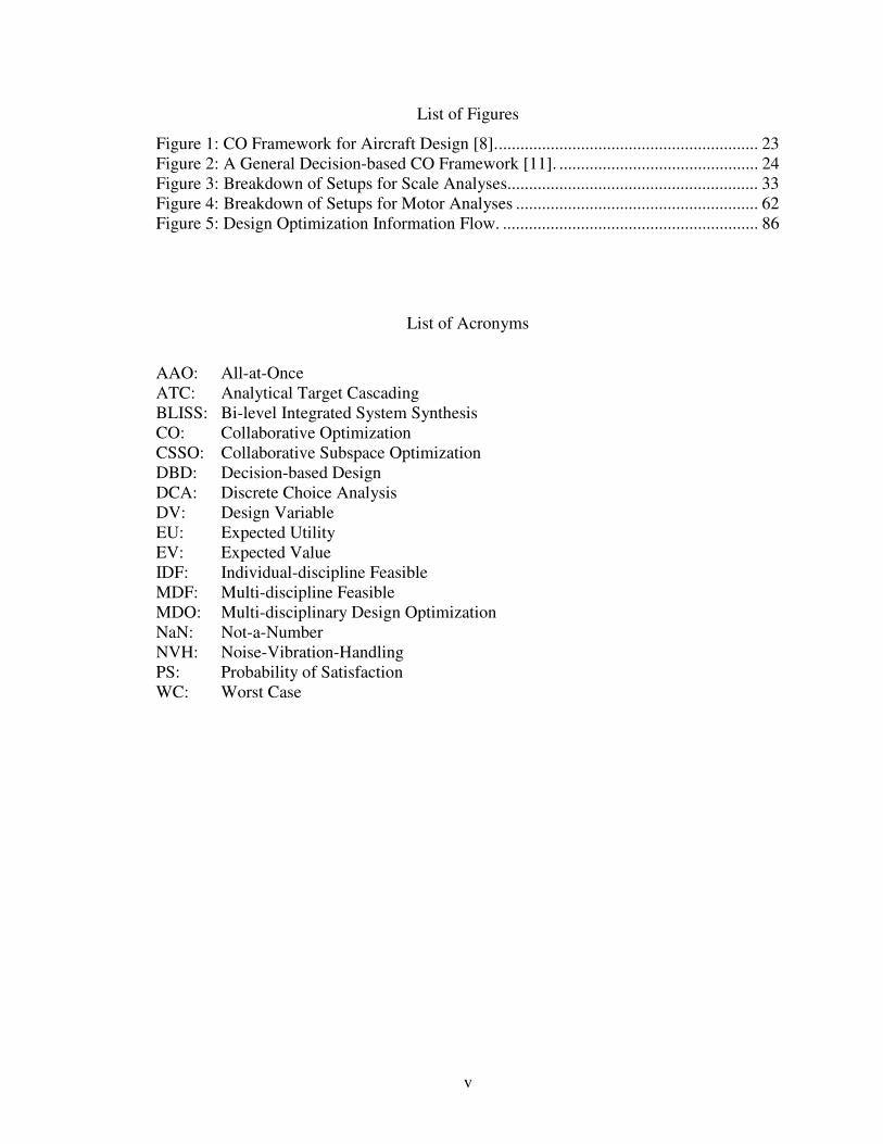
List of Figures

Figure 1: CO Framework for Aircraft Design [8]............................................................. 23 Figure 2: A General Decision-based CO Framework [11]. .............................................. 24 Figure 3: Breakdown of Setups for Scale Analyses.......................................................... 33 Figure 4: Breakdown of Setups for Motor Analyses ........................................................ 62 Figure 5: Design Optimization Information Flow. ........................................................... 86

List of Acronyms

AAO: All-at-Once ATC: Analytical Target Cascading BLISS: Bi-level Integrated System Synthesis CO: Collaborative Optimization CSSO: Collaborative Subspace Optimization DBD: Decision-based Design DCA: Discrete Choice Analysis DV: Design Variable EU: Expected Utility EV: Expected Value IDF: Individual-discipline Feasible MDF: Multi-discipline Feasible MDO: Multi-disciplinary Design Optimization NaN: Not-a-Number NVH: Noise-Vibration-Handling PS: Probability of Satisfaction WC: Worst Case

1

CHAPTER 1: INTRODUCTION

Product design optimization is an important step in the product development

process. An optimal product may be defined as one that meets its performance

requirements with the best economical outlook. In general product design optimization

determines the best values for design variables based on some performance attributes that

satisfy all constraints and maximize some overall objective. In its early stages design

optimization was applied to detailed design problems with simple models that could be

solved by hand. With the invention and advancement of computers, larger and more

complex problems can be handled in a reasonable amount of time. Today design

optimization is used in many stages of the product development process including

conceptual design to evaluate possible concepts and multidisciplinary design to embrace

interests from several departments within an engineering firm simultaneously.

Product design optimization, like other aspects of product development,

continuously changes as new ideas and improved technology surface at an unprecedented

rate. Much advancement in design optimization has focused on solution techniques and

decomposition frameworks. A decomposition framework is a modeling architecture that

allows a complex problem to be broken into more manageable subproblems. For

example, multi-disciplinary design optimization techniques such as collaborative

optimization, analytical target cascading, and concurrent subspace optimization are all

decomposition frameworks. To demonstrate a new technique simple comparisons of the

solution are made with previously accepted techniques to verify proper convergence and

possibly improved performance. New decomposition frameworks attempt to link

2

multiple disciplines to incorporate decisions and goals of each discipline without limiting

the influence of each discipline’s expertise.

With all of the advancements in optimization solution techniques, it seems that

little importance has been placed on the information an engineer must have during the

formulation of a design optimization problem. More information is needed to create

more sophisticated optimization models. For example, maximizing profit requires

information about how the design variables affect demand and cost. Studying the

information requirements can help us explore the tradeoff between information

requirements and solution quality. This thesis attempts to help design engineers formulate

the optimization problem by providing a method of finding similar problems based on a

classification scheme as well as providing insight into the tradeoffs involved in using

different modeling approaches.

A classification scheme will be proposed and demonstrated in an attempt to

standardize the taxonomy used by the optimization community in discussing product

design optimization problems. The goals when developing this classification framework

included both scientific and practical ones. The classification framework helps to

organize and understand design optimization problems, an important step in any scientific

discipline. A standardized taxonomy can assist design engineers when searching for

similar examples previously handled by other engineers. The proposed classification

scheme sorts design optimization problems based on the type of variables being

considered and the objective functions being optimized. It does not focus on the

algorithms used to solve the problems. This classification framework provides a new

perspective that can help design engineers use optimization in the most appropriate way.

3

The second part of the thesis considers the tradeoff between information

requirements and solution quality. Insight into the tradeoffs involved in using different

modeling approaches are accrued by determining the information requirements needed to

solve design optimization problems when formulated using different decomposition and

solution techniques. The information available can greatly affect the effort needed to

formulate the optimization model and the quality of results obtained during an

optimization process. The majority of attention in available literature has been placed on

finding new solution techniques rather than on the quantity of information needed to find

an appropriate solution. Two example problems from previous literature will be

optimized using different modeling approaches and disciplines to study information

requirements and solution quality.

The questions we hope to answer from the computational experiments include the

following: With the information that I have available right now, if I formulate problem P

like example A and get solution X, how much effort will it take to get solution X and

how good is solution X? On the other hand, if I formulate the problem like example B

and get solution Y, what is the difference in effort required and quality compared to

solution X? What other observations can be made from the analysis? What amount of

information was needed to model P like A versus B relative to the quality of the solution?

Chapter 2 provides the relevant background information and literature review of

the optimization field. Chapter 3 describes the methodology used in developing a

classification scheme and analyzing relationships between a knowledge base and

modeling. Chapter 4 details and demonstrates a classification framework for general

product design optimization problems. Chapter 5 includes the analysis of a universal

4

electric motor. Chapter 6 details the analysis of a bathroom scale. Chapter 7 offers a

generalized discussion about the observed connections between heuristics and modeling.

Finally, Chapter 8 summarizes and concludes the thesis.

5

CHAPTER 2: BACKGROUND

Product development has been a lively research area over the last few decades

especially in system level design optimization. Much work has been done to develop

new techniques and frameworks to aid in solving complex optimization problems.

Adding disciplines and increasing problem complexity accented the major limitations of

initial solution techniques thus driving researchers to find alternate approaches [1]. The

growing complexity of optimization problems is forcing engineers to depend more on

powerful software and computer technology, while improvements in computing

technology allow engineers the opportunity to attempt complex problems.

Advancements in computer capabilities and software have helped bridge the gap

between research and industrial applications. For example, software such as iSight,

MAX, and Smart|Coupling can currently integrate several disciplines into one complete

optimization [2, 3]. Third party analysis software such as computational fluid dynamics,

finite element analysis, spreadsheet simulation, and in house code are currently being

integrated through these programs to expand the scope of optimization capabilities. New

research in optimization and improvements in software have generated two major shifts

in the scope of optimization techniques.

First, a shift from single discipline optimization, e.g. structures, to multiple

disciplines within the engineering domain, e.g. performance, structures, and

aerodynamics, occurred. Multiple disciplines meant more objectives to satisfy and

coupling considerations to handle during the optimization process. As a result, several

multidisciplinary design optimization (MDO) techniques such as all-at-once (AAO),

individual-discipline feasible (IDF), and multi-discipline feasible (MDF) approaches

6

were developed [4, 5]. Since then, other MDO solution methods including collaborative

optimization (CO), concurrent subspace optimization (CSSO), and bi-level integrated

system synthesis (BLISS) have been created and demonstrated in example problems [6].

MDO techniques apply various decomposition and coordination methods to facilitate

communication between several disciplines while utilizing common optimization solvers

to find a solution. Sub-optimization functions can be contained within the subsystems,

with appropriate coupling variables linking all the systems and subsystems together, to

ensure a global objective is maintained.

Collaborative optimization (CO) and analytical target cascading (ATC) are two

common frameworks used in multidisciplinary optimization that have been demonstrated

frequently in the last decade. CO is a bi-level optimization method used for non-

hierarchical systems [7-11]. The newer method of ATC, on the other hand, decomposes

a hierarchical system into two or more levels [6, 14-17]. ATC is not directly a

categorization of an MDO technique because it depends on how the problem is

decomposed.

The second shift occurred as a result of the growing popularity of decision-based

design (DBD). Since Hazelrigg [18] introduced a DBD framework for engineering

design, applications have evolved to include decision-making and uncertainty [19-22].

MDO techniques are being applied to the DBD framework in an attempt to handle added

variables from the marketing and manufacturing domains [6,11,16,17]. Many approaches

have been developed and tested on example problems, however, the majority of available

literature detailing these example problems is organized around modeling techniques and

solution methods.

7

To the authors’ knowledge there have been only two classification schemes

related to single product design optimization. The first was a taxonomy for three MDO

decomposition approaches developed by Cramer et al. [5] resulting in the AAO, IDF, and

MDF approaches mentioned previously. The second classification scheme, developed by

Balling and Sobieszczanski-Sobieski [9], was a more general and versatile taxonomy for

the six fundamental approaches of MDO decomposition. The notation in this taxonomy

distinguishes between single and multi-level optimization and whether the analysis is

simultaneous or nested at the system and discipline levels. Both of these classification

schemes focus on the details of the techniques used to solve multi-discipline problems.

In 1979, Graham et al. [12] created a classification scheme that helped generate

ideas for the formulation proposed in this thesis. The three field α/β/γ notation classifies

machine scheduling optimization problems based on various machine environments, job

characteristics, and scheduling objectives, respectively [13].

To the author’s knowledge there has not been any work conducted on evaluating

optimization problems from the information flow perspective used in this research.

Somewhat relevant literature related to the analyses performed in this thesis is found in

Pan and Diaz [23]. Pan and Diaz discuss some inherent difficulties that arise when tightly

coupled design problems are decomposed in a nonhierarchical fashion and solved

sequentially. Sequential optimization is the process of obtaining a solution by first

solving a subproblem, then using the outputs from that subproblem as inputs to a

succeeding subproblem optimization. This process is repeated until all design variables

have been determined.

8

CHAPTER 3: METHODOLOGY

This thesis consists of two activities: the development of a classification scheme

for product design optimization and an investigation of relationships between information

requirements and solution quality. This chapter will discuss the methodology used in

each.

3.1 Classification Scheme

Developing a classification scheme that is general enough to span a large space of

optimization problems requires knowledge of a large space of optimization problems. To

gain this knowledge a literature review of single discipline as well as multi-discipline

optimization frameworks, solution techniques, and examples was conducted. From this

review comparisons were made based on common elements of optimization problems

such as objective functions, constraints, variables, and disciplines involved. Important

categories common to all optimization problems were selected with the intention of

developing a classification scheme that can be used as means for comparing an unsolved

optimization problem at hand with existing examples. These categories are a set of

relevant metrics used in comparing various optimization problems to determine if

existing examples can aid an engineer in solving their own optimization problem.

Extensions to the three main categories were then analyzed for relevance and importance

once the categories were decided on. These extensions included conceptual versus

detailed design, single objective versus multi-objective optimization, and deterministic

versus non-deterministic models.

9

3.2 Computational Experiments

Exploring the tradeoffs between information requirements and the solution quality

was done using computational experiments on two example problems from the literature.

The two example problems, including a bathroom scale and universal electric motor,

were reformulated in several different ways to adjust the number of disciplines,

constraints, objective functions, initial solutions, target values, and sequence used to

solve them. Relation matrices were developed to determine alternate ways of

decomposing the problems and to understand the degree of coupling involved in each

example. A highly coupled system cannot be decomposed into a set of independent

subsystems. The majority of subsystems will have direct dependence on one or more

other subsystems. A weakly coupled system, on the other hand, can be decomposed into

a set of subsystems with little dependence on other subsystems.

To study the tradeoff between information requirements and solution quality, the

scope (i.e. number of disciplines) was increased by formulating a profit maximization

problem that adds the marketing discipline to the engineering discipline. This requires

more information but should yield a more profitable solution. Variations in constraints

were generally related to the decomposition and scope of the problem. Adding the

marketing discipline adds more constraints in an attempt to simultaneously satisfy more

requirements. However, in some cases equality constraints were removed and replaced

with target values in the objective function.

Many of the optimization setups were single discipline optimizations involving

just engineering. For these cases the design variables were found using an engineering

10

optimization model. The results were then evaluated by estimating the profitability,

which required a price optimization.

When a problem is decomposed in different ways the constraints directly relevant

to each subsection of the decomposition change depending on what variables are included

in that respective subsection. Objective functions were changed in many different ways

including single to multi-objective, weighting, and target settings. Finally, the sequence

of solving the optimization was changed to determine the impact on solution quality,

feasibility, and computational effort. Various sequences, if possible, were developed and

solved.

For all the different variations described above, appropriate optimization models

were created and solved using the optimization toolbox in MATLAB 7.0.4™. The

MATLAB function fmincon was used in all cases to minimize the constrained

optimization. In most cases default MATLAB settings were used for the constrained

minimization problems, however, there were some cases where the number of allowable

function calls was increased and the convergence criteria softened. The results were then

compared and analyzed in an attempt to quantify the solution quality of different

optimization models.

11

CHAPTER 4: A CLASSIFICATION FRAMEWORK

Research on design optimization has developed and demonstrated a variety of

modeling techniques and solution methods, including techniques for multidisciplinary

design optimization, and these approaches are beginning to migrate into product

development practice. Software tools are appearing to assist with the optimization task.

However, the complexity of the optimization problems being considered continues to

increase because changing business strategies stress the importance of concurrent

engineering and considering multiple disciplines simultaneously. This chapter presents a

classification framework based on the examination of various design optimization

problems from the perspective of information requirements and objectives. We are not

directly concerned with decomposition or modeling techniques nor do we limit our

classification to MDO problems. The generality of the proposed classification allows

even the most basic optimization problems to be classified.

Our goals when developing this classification framework included both scientific

and practical ones. First, this classification framework helps us to organize and

understand design optimization problems, an important step in any scientific discipline.

While this classification framework is not the only conceivable scheme, we believe that it

concisely captures the most important attributes while remaining open to including other

attributes in the future if so desired. Second, this classification framework provides

practical help for design engineers considering design optimization. Using this scheme, a

design engineer can locate similar design optimization problems, which can be useful

guides for formulating a new problem. Moreover, the set of similar design optimization

problems indicates the range of potential solution techniques. Of course, the design

12

engineer must still choose a problem formulation and a solution technique. This

classification framework does not replace modeling skill, but it does provide information

that can help one develop it.

The remainder of the chapter proceeds as follows. After defining some key terms

used in the chapter, we present the classification framework and then use available

examples to demonstrate it.

4.1 Definitions

Many areas within a firm can influence the product development process.

Engineering is obviously the basis of design while manufacturing and marketing are a

major part of concurrent engineering. The engineering domain represents the perspective

of design engineers and concerns about the product design and product performance. The

manufacturing domain represents the perspective of manufacturing personnel and

concerns about the manufacturing process and the corresponding metrics. The marketing

domain represents the perspective of the product manager and concerns about finances,

customer preferences, and demand.

Design optimization problems have three primary features: variables, constraints,

and objective functions. Our classification framework will consider only variables and

system level objectives. Secondary objectives, which may appear in constraints or

subsystems, do not affect the classification scheme. Constraints are important because

they can influence the choice of an optimization solver based on whether the constraints

are linear, nonlinear, equality, or inequality constraints. However, constraints are

13

generally created during the modeling process. Our classification framework is meant to

describe the fundamental problem, not the model details.

Due to the nonconformity of terminology in design research, the following

definitions are given along with possible synonyms to avoid any confusion.

4.1.1 Product Scope

The classification framework distinguishes between single product design

optimization and product family optimization. Definitions for each of the two product

types are given for clarity, however, only single-product design problems are treated in

this thesis. Future work will extend this classification scheme to product families.

Single Product: This is a product that is designed with no regard to similar products.

Component sharing and interconnection with other products do not influence the

design decisions.

Product Family [24]:

1. A set of common elements, modules, or parts from which a stream of derivative

products can be efficiently developed and launched.

2. A collection of common elements, especially the underlying core technology,

implemented across a range of products.

3. A collection of assets (i.e., components, processes, knowledge, people and

relationships) that are shared by a set of products.

14

4.1.2 Variables

Variables are sometimes referred to as parameters, design variables, and design

parameters [25]. A designer must select the values for variables. Optimization is used to

help find appropriate values of variables. The following three definitions refer to more

specific types of variables.

Engineering Variables: These are variables specific to the product being designed.

Typical engineering variables include product geometry, features, and material

selection.

Manufacturing Variables: These are variables specific to the manufacturing domain.

Every facility will have different manufacturing variables specific to the machine

types and facility layout. Examples include number of machines, time allotment per

machine, number of operations per part, force and energy requirements, feed rate, and

depth of cut.

Price Variable: This variable is the price of the product or system being designed.

Pricing is a critical but complex issue. For a new product, a successful pricing

approach first determines the price that customers can be convinced to pay for the

product concept, and then the firm designs a satisfactory product that can be

manufactured profitably at the expected sales volume [26]. While the initial pricing

strategy may be used to set a cost target for the product design, the product price will

certainly change over time as the firm’s pricing strategy influences their response to

15

market forces. The product development team does not need to make pricing

decisions that have not yet arrived. However, optimizing product profitability at the

design stage requires understanding what the firm is likely to do. If alternative

strategies are feasible (such as skim pricing or penetration pricing), the team may

want to evaluate these strategies, since they control future prices.

4.1.3 Objective Functions

Design optimization (especially MDO) can include several subproblems

depending on the system being designed. The classification framework considers only

the system level objectives. The classification framework covers single objective as well

as multi-objective optimization problems at the system level.

Attribute-based: These objective functions are related to product performance or

product characteristics (i.e. attributes). For the purposes of this classification

framework an attribute is a quantitative measure related to the object or system being

designed. The objective is to maximize or minimize an attribute level, usually a

performance measure, based on the product being designed. Although uncommon, it

is possible to utilize demand information in the attribute-based objective function but

it is not a requirement. Examples: minimize weight, minimize size, minimize stress,

and maximize range. Alternatively, the objective may be to minimize the deviation

from a target attribute value.

16

Cost-based: These objective functions are related to the engineering and

manufacturing domains. The goal is to minimize the overall cost of the product based

on one or more cost models. Generally this type of optimization will be more

complex than the attribute-based objective because cost models will be necessary

along with the design models. While one can consider a cost objective to be a

performance measure equivalent to any attribute-based objective, we treat cost

separately because product performance and product cost are fundamentally different

and very important objectives, as discussed by Smith and Reinertsen [27]. Therefore

it is useful to the designer if a distinction is made between the two types of objectives.

Similar to the attribute-based objective function this can include situations where the

objective is to minimize the deviation from a cost target. Demand can again be

utilized as a weighting method in this objective but is not required.

Profit-based: These objective functions are directly related to the marketing domain.

The goal of the optimization is to maximize the design value based on demand

information. Although not stated explicitly in the classification it can be assumed that

any profit-based objective will require some type of demand model. Another step in

complexity is seen through the profit-based models, in comparison to the attribute-

based and cost-based models, because more model evaluations are required for this

type of optimization. Examples: maximize revenue, maximize profit, maximize

expected utility of profit, maximize net present value, and maximize return on

investment.

17

4.2 Classification Framework

Three main categories become apparent when considering design optimization

problems. Our classification framework sorts design optimization problems based on the

following three characteristics: problem scope (i.e. single product versus product family),

the variables that need to be decided (i.e. engineering, manufacturing, or price), and the

system level objective function (or functions) of the optimization problem (i.e. attribute-

based, cost-based, or profit-based).

To explain the classification framework, we will begin with the most basic types

of deterministic optimization problems involving only a single objective function.

Subsequent paragraphs will discuss problems with multiple objectives. After that, we

will present a modifier to the objective function to describe typical methods of dealing

with uncertainty.

The classification framework categorizes design problems using three fields

corresponding to the three characteristics mentioned above. The first field notes the

number of products. The second field notes the types of variables. The third field notes

the type of objective function (or functions). Designing a single product with a single

system level objective can include twelve possible optimization framework combinations.

Six of the twelve combinations are more likely to be used due to the relationship between

the objective function and the variables considered. For example, if the design process

includes only engineering variables, then maximizing profit would not be a typical

objective function since maximizing profit or the expected utility of profit would include

the price variable. The twelve combinations for single objective optimization problems

are shown in Table 1 with the six most logical in boldface.

18

The product type entry in field one can be either single product (S) or product

family (F). Variables present in the optimization, shown in field two, may include

engineering variables (E), manufacturing variables (M), or a price variable (P). Field

three displays the objective functions for each combination of variables, which include

attribute-based objectives (A), cost-based objectives (C), and profit-based objectives (Π).

Single Objective

Field #

1 2 3 Product Type Variables Included System Objective

S E A Single Eng. Attribute-based

S E C Single Eng. Cost-based

S E Π Single Eng. Profit-based

S EM A Single Eng. & Mfg. Attribute-based

S EM C Single Eng. & Mfg. Cost-based

S EM Π Single Eng. & Mfg. Profit-based

S EP A Single Eng. & Price Attribute-based

S EP C Single Eng. & Price Cost-based

S EP ΠΠΠΠ Single Eng. & Price Profit-based

S EMP A Single Eng., Mfg. & Price Attribute-based

S EMP C Single Eng., Mfg. & Price Cost-based

S EMP ΠΠΠΠ Single Eng., Mfg. & Price Profit-based

Table 1: Combinations of Single Product Optimization with a Single Objective.

The above classification framework is easy to use and self-explanatory. For

instance, if a problem is classified as type S-E-A, one can immediately know that the

optimization problem is for a single product, it has only engineering variables, and has an

attribute-based objective.

The classification framework also includes multi-objective design optimization

problems, resulting in eight more common combinations. The third field of the

classification is further divided into two subfields (i.e. positions within the third field).

19

The first subfield may contain the entry “A” or “C.” The second field on the other hand

can be either “A”, “C”, or “Π” to specify what other objectives are present.

The classification of an optimization problem with two or more attribute-based

objectives would contain “AA” in the third field (e.g. S-E-AA or S-EM-AA). If “AC”

appears in the third field of the classification then there are two or more attribute-based

and cost-based objectives. Similarly, “AΠ” is used for the multi-objective case where

attribute-based and profit-based objectives are present. The latter can be seen in

multidisciplinary design optimization techniques such as ATC and CO when the multi-

objective function is to minimize the deviation between attribute targets while

maximizing profit [16, 17]. Note the specific number of objectives is not specified in the

multi-objective case. The formulation of the objective function, as well as the choice of

optimization program, may alter depending on the number of objectives (e.g., two versus

four objectives) but from the perspective of the proposed classification scheme these

differences are minor. Distinguishing between a single objective optimization and a

multi-objective optimization plays a much larger role in selecting a solution technique

than the difference between two objectives and four objectives.

The classification scheme also ignores the details of how a multi-objective

problem is formulated. Multiple objectives are often formulated into a single objective

function, for example minimizing the deviation between several targets and responses,

but this distinction is too detailed when compared to the perspective used in developing

the classification scheme.

The occurrence of a “CΠ” classification is unlikely because cost models are

generally inputs to the profit model though this multi-objective problem is technically

20

feasible. The sixteen possible combinations are shown in Table 2 with the eight most

typical combinations in bold.

Multi-Objective

Field #

1 2 3 Product Type Variables Included System Objective

S E AA Single Eng. Attribute-based

S E AC Single Eng. Att. & Cost-based

S E CC Single Eng. Cost-based

S EM AA Single Eng. & Mfg. Attribute-based

S EM AC Single Eng. & Mfg. Att. & Cost-based

S EM CC Single Eng. & Mfg. Cost-based

S EP AA Single Eng. & Price Attribute-based

S EP AC Single Eng. & Price Att. & Cost-based

S EP AΠΠΠΠ Single Eng. & Price Att. & Profit-based

S EP CC Single Eng. & Price Cost-based

S EP CΠ Single Eng. & Price Cost & Profit-based

S EMP AA Single Eng., Mfg. & Price Attribute-based

S EMP AC Single Eng., Mfg. & Price Att. & Cost-based

S EMP AΠΠΠΠ Single Eng., Mfg. & Price Att. & Profit-based

S EMP CC Single Eng., Mfg. & Price Cost-based

S EMP CΠ Single Eng., Mfg. & Price Cost & Profit-based

Table 2: Combinations of Single Product Optimization with Multiple Objectives.

Deterministic models are preferred by engineers due to the simplicity of

formulating and solving them. Unfortunately, it is a well known fact that the real world

is not deterministic. Therefore, it is important to include uncertainty in the classification

framework. An objective function subclass, including five methods of dealing with

uncertainty, categorizes and clarifies optimization problems further. The first method of

dealing with uncertainty is ignoring it, thus the problem is a deterministic optimization

problem. Four other common methods include expected value (EV), expected utility

(EU), worst-case (WC), and probability of satisfaction (PS). Although there are

21

variations to the methods mentioned above (such as the Hurwicz criteria and maximum

likelihood criteria), we believe the most common forms are accounted for.

The classification framework represents the uncertainty subclass using a subscript

on the objective function terms in the third field. Deterministic objective functions would

have no subscript in the third field while the four common methods for dealing with

uncertainty described above would include a subscript of EV, EU, WC, or PS

respectively. For example, the classification S-E-AWC is used for problems that address a

single product, have engineering variables, and optimize the worst-case performance.

The framework is deployed in the next section to classify available examples.

Engineers will be able to use available examples to perform a case-based search and find

design problems that are similar based on the three fields of the classification scheme and

compare the different solution techniques previous designers used in solving the problem.

4.3 Examples

Available examples of various optimization problems, including MDO problems,

will be classified using the proposed framework. The MDO problems used for

demonstrating the framework were solved using either ATC or CO techniques.

An S-E-A type optimization is the most basic because it involves only the

engineering domain. Therefore, the equations used to model this type of optimization

rely only on principles of engineering science. First a general optimization problem is

discussed followed by another example that employs one of the afore-mentioned MDO

techniques.

22

A simple single discipline example of designing a fingernail clipper can be found

in Otto and Wood [28]. In this example a model is formulated to represent finger force.

The variables included in this model are finger force, cutting force at the blade, length of

lever arm, distance to the blades, nail thickness, width of blade, and blade height. The

deterministic attribute-based objective chosen in designing the fingernail clipper is to

minimize the finger force required subject to stress and dimension constraints. It can

easily be seen by looking at the variables involved that only engineering variables are

included for the design of a single fingernail clipper. Thus, this problem can be classified

as type S-E-A. Cost and manufacturing concerns are not present in the formulation

although it is possible to extend this problem to include such domains.

Kroo et al. [8] present a system level aircraft design problem. The global

objective function is to maximize range under the influence of an aerodynamics

subsystem, a structures subsystem, and a performance subsystem. Range is an attribute

of the system to be designed, which corresponds to the “A” in the classification. The

variables in this problem are all related to the plane’s design and include wing geometry,

wing weight, twist angle, aspect ratio, gust loading, and lift-to-drag ratio, all of which

affect range. This is a deterministic S-E-A problem because no distributions are applied

to the input variables. Figure 1 shows the CO framework applied to solve this aircraft

design problem.

23

Figure 1: CO Framework for Aircraft Design [8].

The CO framework in this example clearly shows what variables are present

during the optimization as well as the disciplines influencing the system level design.

Notice the classification framework is not directly related to how the problem is divided

or what disciplines within engineering are included. Sobieski and Kroo [10], Kim et al.

[14, 15], Otto and Wood [28], and McAllister and Simpson [29] demonstrate other

examples of S-E-A type optimization problems.

Although a fingernail clipper and aircraft design problem in the above examples

intuitively seem very different, the difficulty in solving them is not all that different. The

fingernail clipper is a detailed design problem while the aircraft wing is more conceptual.

The aircraft design problem could have been formulated and solved as an AAO instead of

using the collaborative optimization, in which case the two examples would appear to

have a greater similarity. When a problem can be decomposed and modeled in different

ways, a design engineer would probably want to see examples of several different

methods to find the most appropriate one. Therefore, multiple examples of techniques

24

based on similar problems seem more useful especially when dealing with a somewhat

complex design problem.

Next, an example of an S-EP-Π type optimization problem is examined. Gu et al.

[11] details an aircraft concept-sizing problem to maximize profit under the influence of

engineering variables and a price variable. The authors chose to assume the utility of

profit to be profit itself thus treating it as a deterministic problem for calculation

purposes. If uncertainty were accounted for through a utility function this problem would

be classified as S-EP-ΠEU. Figure 2 shows the general layout of the decision-based

collaborative optimization approach.

Figure 2: A General Decision-based CO Framework [11].

The engineering variables included in this single aircraft optimization example

consist of aspect ratio, wing area, fuselage length, fuselage diameter, density of air at

cruise altitude, cruise speed, and fuel weight. The price variable is also part of the

optimization problem. In a profit-based optimization problem the cost models are present

as inputs to a profit function but do not affect the classification framework because it is

25

not a system level objective. The cost model term is present in the classification

framework only for systems with a cost-based objective. Another example of a type S-

EP-Π optimization can be found in Kumar et al. [6].

Next, an example is taken from Sues et al. [31] to demonstrate the uncertainty

sub-class within the classification framework. This shape optimization of an airplane

wing includes seven engineering variables related to the wing geometry. Values for

aspect ratio, taper ratio, semi span wingtip incidence, structure skin thickness, structure

span thickness, and wing sweep all need to be decided. The global objective of this

single wing shape optimization is to maximize expected cruise range. Uncertainty

appears through random distributions on all of the design variables to account for

inconsistencies in the manufacturing processes. This example can be classified as type S-

E-AEV. Several other examples dealing with uncertainty can be found in Sues et al. [31].

An example of type S-EP-ΠEU can be found in [30].

Finally, a multi-objective optimization example will be classified using the

framework. Azarm and Narayanan [32] discuss a multi-objective example regarding the

design of a fleet of ships. The objectives of this example include minimizing construction

and operating costs and maximizing the cargo capacity. The engineering variables

present in the model of this optimization include: breadth, depth, deadweight, length,

number of ships, draft, utilization factor, speed, and displacement. Due to the conceptual

nature of this optimization problem, specific manufacturing construction variables were

not considered. Manufacturing costs, however, were accounted for in the cost models.

This problem can be classified as type S-E-AC. The “A” denotes the presence of an

attribute-based objective (maximize cargo capacity) while the “C” denotes the presence

26

of a cost-base objective (minimize construction and operating costs). Tappeta and

Renaud [33] present an aircraft concept-sizing problem that can be classified as S-E-AA.

The problem has two attribute-based objective functions: minimize mass and maximize

range.

Classification Reference # Description

S-E-A 1 Launch Vehicle

S-E-A 2 Aircraft Engine

S-E-A 8 Aircraft Design

S-E-A 10 Aircraft Wing

S-E-A 14 Chassis Design

S-E-A 15 Chassis Design

S-E-A 28 Finger Nail

S-E-AEV 31 Airplane Wing

S-E-C 1 Launch Vehicle

S-E-C 2 Aircraft Engine

S-EP-Π 11 Aircraft Concept

S-EP-ΠEU 6 Suspension

S-EP-ΠEU 30 Universal Motor

S-E-AA 33 Aircraft Concept

S-E-AC 32 Fleet of Ships

S-EP-AΠ 16 Weight Scale

Table 3: Classified Examples from Literature.

27

CHAPTER 5: ANALYSIS OF A BATHROOM SCALE

Modeling is a difficult task that generally requires experience, above and beyond

academic knowledge, to truly perfect [34]. Decisions during the modeling process

include things like objective function type, constraint type, decomposition method,

optimization algorithms, and number of disciplines (i.e. scope). The next two chapters

take a closer look at objective function formulation, demand modeling, decomposition,

and information requirements.

This chapter begins the second part of the thesis, which addresses the questions

raised in Chapter 1: With the information that I have available right now, if I formulate

problem P like example A and get solution X, how much effort will it take to get solution

X and how good is solution X? On the other hand, if I formulate the problem like

example B and get solution Y, what is the difference in effort required and quality

compared to solution X? What other observations can be made from the analysis? What

amount of information was needed to model P like A versus B relative to the quality of

the solution? Realizing that different models lead to different solutions is intuitive. We

use computational experiments to get additional insight into the tradeoffs between

information requirements and solution techniques.

A bathroom scale example, originally developed by Michalek et al. [16], will be

used to help analyze and answer the questions mentioned in the introduction. The

example in [16] was used to demonstrate the multi-disciplinary design optimization

(MDO) technique known as analytical target cascading (ATC). A simple comparison of

the ATC and a disjoint approach was given to show the effectiveness and correctness of

the ATC approach. A disjoint approach is when an engineering optimization is solved

28

first to determine all the engineering variables followed by a marketing optimization to

determine price. No mention of information requirements or difficulty in programming

the two approaches is given.

5.1 Original Model Formulation

The bathroom scale design problem includes fourteen design variables [x1, …,

x14], six customer attributes [z1, …, z6], thirteen fixed model parameters [y1, …, y13], and

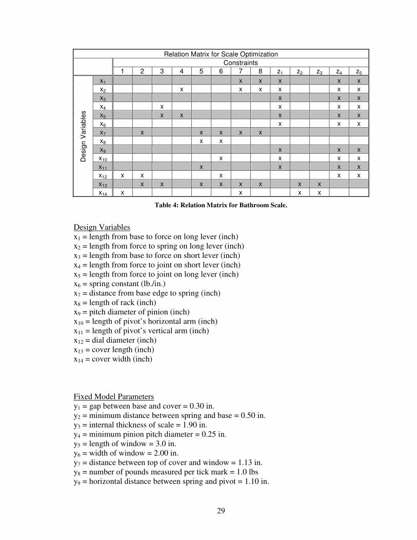
eight constraints. The selection reasoning and derivation of the variables and equations

for this model can be found in [16]. A relation matrix, shown in Table 4, shows the

degree of coupling between design variables, constraints, and attributes (which are used

as constraints in the all-at-once approach). The rows include all fourteen design

variables while the columns include the eight geometric constraints along with the five

customer attributes. A constraint or attribute with an “x” indicates it is a function of the

variable xi corresponding to row i where that respective “x” appears. The following

matrix shows the degree of coupling in this example to be moderate, meaning it is not

fully coupled nor is it completely uncoupled. The nomenclature and equations for the

design variables, fixed model parameters, customer attributes, and constraints are also

listed below.

29

Relation Matrix for Scale Optimization Constraints

1 2 3 4 5 6 7 8 z1 z2 z3 z4 z5

x1 x x x x x x2 x x x x x x x3 x x x x4 x x x x x5 x x x x x x6 x x x x7 x x x x x x8 x x x9 x x x x10 x x x x x11 x x x x x12 x x x x x x13 x x x x x x x x

Des

ign

Var

iabl

es

x14 x x x x

Table 4: Relation Matrix for Bathroom Scale.

Design Variablesx1 = length from base to force on long lever (inch) x2 = length from force to spring on long lever (inch)x3 = length from base to force on short lever (inch) x4 = length from force to joint on short lever (inch)x5 = length from force to joint on long lever (inch) x6 = spring constant (lb./in.) x7 = distance from base edge to spring (inch) x8 = length of rack (inch) x9 = pitch diameter of pinion (inch) x10 = length of pivot’s horizontal arm (inch) x11 = length of pivot’s vertical arm (inch) x12 = dial diameter (inch) x13 = cover length (inch) x14 = cover width (inch)

Fixed Model Parametersy1 = gap between base and cover = 0.30 in. y2 = minimum distance between spring and base = 0.50 in. y3 = internal thickness of scale = 1.90 in. y4 = minimum pinion pitch diameter = 0.25 in. y5 = length of window = 3.0 in. y6 = width of window = 2.00 in. y7 = distance between top of cover and window = 1.13 in. y8 = number of pounds measured per tick mark = 1.0 lbs y9 = horizontal distance between spring and pivot = 1.10 in.

30

y10 = length of tick mark plus gap to number = 0.31 in. y11 = number of pounds that number length spans = 16.00 lbs y12 = aspect ratio of number = 1.29 y13 = minimum allowable distance of lever at base to centerline = 4.00 in.

Customer Attributes

z1 = weight capacity (lbs) = ( )( )

( ) ( )( )6 9 10 1 2 3 4

11 1 3 4 3 1 5

4 x x x x x x x

x x x x x x x

π + +

+ + +

z2 = aspect ratio = 13

14

x

x

z3 = platform area (in2) = 13 14x x

z4 = tick mark gap (in.) = 12

1

x

zπ

z5 = number size (in.) = 11 12

101

11

12 1

2 tan2

21 tan

y xy

z

y

y z

π

π

⎛ ⎞⎛ ⎞ ⎛ ⎞−⎜ ⎟⎜ ⎟ ⎜ ⎟

⎝ ⎠⎝ ⎠⎝ ⎠⎛ ⎞⎛ ⎞

+⎜ ⎟⎜ ⎟⎝ ⎠⎝ ⎠

z6 = price ($)

Constraints and Bounds on Design Variables

1. 12 14 12 0x x y− + ≤

2. 12 13 1 7 92 0x x y x y− + + + ≤

3. 4 5 13 12 0x x x y+ − + ≤

4. 5 2 0x x− ≤

5. 7 9 11 8 13 12 0x y x x x y+ + + − + ≤

6. ( ) 1213 1 7 7 9 10 82 0

2

xx y y x y x x

⎛ ⎞− − + − − − − ≤⎜ ⎟

⎝ ⎠

7. ( ) ( )2

2 2 14 11 2 13 1 7

22 0

2

x yx x x y x

−⎛ ⎞+ − − − − ≤⎜ ⎟

⎝ ⎠8. ( ) ( )

2 2213 1 7 13 1 22 0x y x y x x− − + − + ≤

x1 x2 x3 x4 x5 x6 x7 x8 x9 x10 x11 x12 x13 x14

LB 0.125 0.125 0.125 0.125 0.125 1 0.5 1 0.25 0.5 0.5 1 1 1 UB 36 36 24 24 36 200 12 36 24 1.9 1.9 36 36 36

Units in. in. in. in. in. lb./in. in. in. in. in. in. in. in. in.

Table 5: Bounds on Engineering Design Variables.

31

z1 z2 z3 z4 z5 z6

LB 200 0.75 100 0.063 0.75 10 UB 400 1.33 140 0.188 1.75 30

Units lbs. - in2 in. in. $

Table 5: Bounds on Product Attributes.

Marketing Related Models

The profit model is a basic model that incorporates demand (q), price (p), variable

cost (cv), and investment cost (ci). Many marketing models superior to this can be found

but for the sake of this analysis the model shown below will suffice.

( )v iq p c cΠ = − − (5.1)

The demand model was developed using discrete choice analysis (DCA) and a

market survey. The total demand is population size multiplied by the probability that a

consumer will select a particular design (i.e. estimated market share). Equation 5.2

shows the common DCA equation developed in [35, 36].

( )

1

1

1

1

( )

v v

K

k Kkk

q sP se e

s population size

z pν

−

−

=

⎡ ⎤= = +⎣ ⎦=

= Ψ + Ψ∑

(5.2)

The attraction value “ν” is simply the summation of the beta values calculated from the

spline functions for each attribute value and price. The spline functions are shown in

Appendix A.

32

5.2 Optimization Setups

Seven different setups are created using the scale example in order to have a basis

for comparing the information requirements and solution quality. The main goal of each

setup is to create a product that will yield the most profit for a company. In general,

Setups 1-6 do this using a disjoint two-step process. The first step is to optimize the

engineering discipline with the assumption that marketing supplied appropriate target

values. The second step is to take the result of step 1, along with customer demand and

cost models, and determine a price to maximize profit. The problem is bounded by the

eight geometric constraints mentioned above. Setup 7 is a joint optimization linking

marketing and engineering. The objective is again to maximize profit but this time

marketing decisions are made at the same time as the engineering decisions. This

optimization problem is bounded by the eight geometric constraints as well as upper and

lower limits on the six customer attributes. Figure 3 offers a clearer distinction between

the seven setups used.

33

Figure 3: Breakdown of Setups for Scale Analyses.

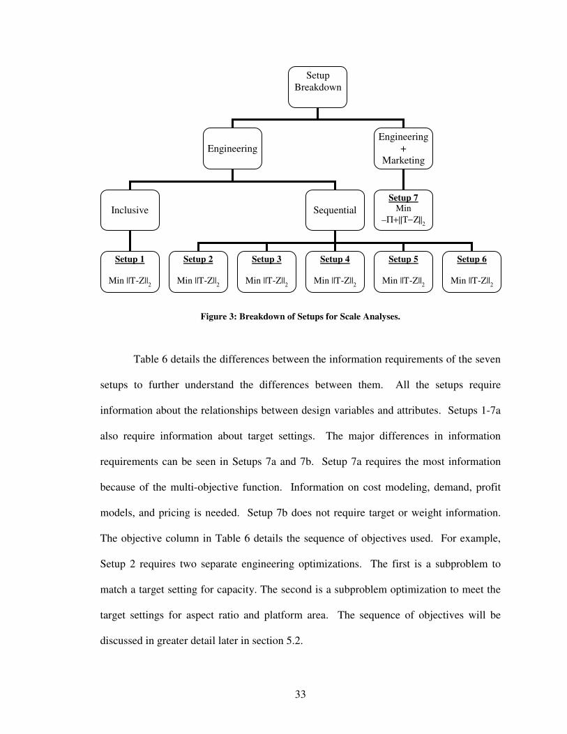
Table 6 details the differences between the information requirements of the seven

setups to further understand the differences between them. All the setups require

information about the relationships between design variables and attributes. Setups 1-7a

also require information about target settings. The major differences in information

requirements can be seen in Setups 7a and 7b. Setup 7a requires the most information

because of the multi-objective function. Information on cost modeling, demand, profit

models, and pricing is needed. Setup 7b does not require target or weight information.

The objective column in Table 6 details the sequence of objectives used. For example,

Setup 2 requires two separate engineering optimizations. The first is a subproblem to

match a target setting for capacity. The second is a subproblem optimization to meet the

target settings for aspect ratio and platform area. The sequence of objectives will be

discussed in greater detail later in section 5.2.

Setup Breakdown

EngineeringEngineering

+ Marketing

Inclusive Sequential Setup 7

Min –Π+||Τ−Ζ||

2

Setup 2

Min ||T-Z||2

Setup 3

Min ||T-Z||2

Setup 4

Min ||T-Z||2

Setup 5

Min ||T-Z||2

Setup 6

Min ||T-Z||2

Setup 1

Min ||T-Z||2

34

Setup # Classification Objective Information

Requirements Outputs

1 S-E-AA Meet all Targets DV Attributes, Targets DV: x1 – x14

2 S-E-A

S-E-AA Capacity

Ratio & Area DV Attributes,

Targets DV: x1 – x14

3 S-E-A

S-E-AA S-E-AA

Capacity Ratio & Area

Gap & Number

DV Attributes, Targets

DV: x1 – x14

4 S-E-AA S-E-A

Ratio & Area Capacity


DV: x1 – x14

5 S-E-AA S-E-A

S-E-AA

Ratio & Area Capacity

Gap & Number


DV: x1 – x14

6 S-E-AA S-E-AA

Gap & Number Ratio & Area


DV: x1 – x14, Price

7a S-EP-AΠ Profit & Targets

DV Attributes, Targets, Weights, Costs, Attr. Demand Price Demand

Profit Model

DV: x1 – x14, Price

7b S-EP-Π Profit DV Attributes, Costs,

Attr. Demand DV: x1 – x14,

Price

Table 6: Breakdown of Seven Scale Setups.

The seven setups were solved using the fmincon function included in the

optimization toolbox in MATLAB™. Within each setup various other parameters are

changed as well such as weighting coefficients and initial solutions. The same seven

initial solutions, shown in Table 7, were used for each of the seven setups. The

feasibility of each initial solution was determined by entering the values into a

spreadsheet model to check for constraint violation prior to running any optimizations.

Initial solution 1 is the optimal result of the ATC approach used in [16]. The other six

initial solutions were arbitrarily determined using trial and error in a spreadsheet model.

35

Initial Solutions for Engineering Optimization Initial Solution Number Design

Variables 1 2 3 4 5 6 7

x1 2.30 18.00 1.00 5.00 1.00 3.39 3.00

x2 8.87 18.00 1.00 10.00 7.00 7.79 8.50x3 1.34 12.00 1.00 12.00 1.00 1.40 1.34x4 1.75 12.00 1.00 5.00 3.00 1.49 1.75

x5 0.41 18.00 1.00 5.00 5.00 0.88 0.41x6 95.70 95.50 1.00 9.00 60.00 95.10 95.70x7 0.50 6.00 1.00 2.00 2.00 0.50 0.50x8 7.44 18.00 1.00 9.00 6.00 6.91 7.44

x9 0.25 12.00 1.00 1.00 1.00 0.30 0.25x10 0.50 1.00 1.00 1.00 3.00 0.55 0.50x11 1.90 1.00 1.00 1.00 1.00 1.84 1.90x12 9.34 18.00 1.00 10.00 7.00 9.33 9.34x13 11.54 18.00 1.00 15.00 11.00 11.53 11.54

x14 11.57 18.00 1.00 18.00 10.00 11.08 11.57

Feasible? NO NO NO YES NO YES NO

Table 7: Seven Initial Solutions Used in All Seven Setups.

5.2.1 Setup 1: Engineering Optimization

For the first setup, an optimization of the scale is performed using the original

fourteen engineering variables with the attribute targets set as the most preferred level of

each attribute based on a customer survey (see Appendix A). All of the geometric

constraints (1-8) were applied as well as the upper and lower bounds on the design

variables. The objective is to minimize the l2 norm of the deviation between target (T)

and response (Z) values. The procedure can be depicted as follows.

Minimize 2

( ) ( )f x w T Z= −

With respect to [x1, …, x14] (5.3)

Subject to: Constraints 1-8; xLB ≤ x ≤ xUB

The optimization was then repeated with different target values and initial

solutions. Target values were adjusted thrice. The first adjustment changed the targets to

36

the actual attainable attribute levels found using the ATC approach detailed in Michalek

et al. [16]. The second adjustment changed the attribute targets to the marketing

optimization result mentioned in Michalek et al. [16]. Finally, the target attributes were

set as the optimal values obtained through my own disjoint marketing optimization (see

Appendix C). The four target setting values are shown in Table 8.

Attributes Target # z1 z2 z3 z4 z5

1 300 1 120 0.125 1.75 2 254 0.997 133 0.116 1.33 3 283 0.946 124.2 0.136 1.75 4 288 0.9285 130.24 0.156 1.75

Table 8: Target Settings Used in Setup 1.

In practice the only target values that a designer will have knowledge of a priori

will be from a marketing survey, which is the first target setting mentioned above. The

other two settings were used to determine the sensitivity that target settings had, if any, to

the solution.

5.2.2 Setup 2: Sequential Engineering Optimization

For this setup the engineering optimization described in Setup 1 is broken down

into three sequential optimizations. The objective functions used in each sequential

optimization again minimize the l2 norm of the deviation between the target and response

vectors as shown in equation 5.4. Target 1 from Table 8 is used for all the sequential

engineering optimizations.

min2

f T Z= − (5.4)

The first optimization determines design variables x1-x6 and x9-x11 while meeting the

target for capacity (z1). The only constraint applied during this optimization is constraint

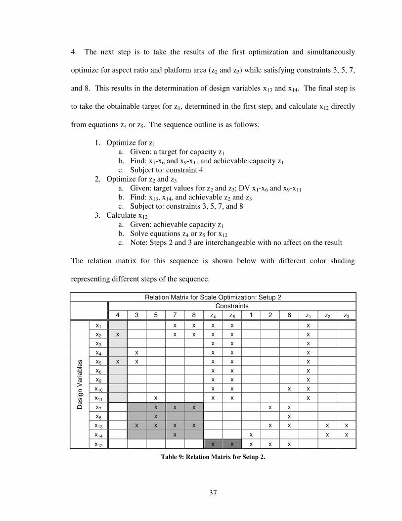
37

4. The next step is to take the results of the first optimization and simultaneously

optimize for aspect ratio and platform area (z2 and z3) while satisfying constraints 3, 5, 7,

and 8. This results in the determination of design variables x13 and x14. The final step is

to take the obtainable target for z1, determined in the first step, and calculate x12 directly

from equations z4 or z5. The sequence outline is as follows:

1. Optimize for z1

a. Given: a target for capacity z1

b. Find: x1-x6 and x9-x11 and achievable capacity z1

c. Subject to: constraint 4 2. Optimize for z2 and z3

a. Given: target values for z2 and z3; DV x1-x6 and x9-x11

b. Find: x13, x14, and achievable z2 and z3

c. Subject to: constraints 3, 5, 7, and 8 3. Calculate x12

a. Given: achievable capacity z1

b. Solve equations z4 or z5 for x12

c. Note: Steps 2 and 3 are interchangeable with no affect on the result

The relation matrix for this sequence is shown below with different color shading

representing different steps of the sequence.

Relation Matrix for Scale Optimization: Setup 2 Constraints

4 3 5 7 8 z4 z5 1 2 6 z1 z2 z3

x1 x x x x x x2 x x x x x x x3 x x x x4 x x x x x5 x x x x x x6 x x x x9 x x x x10 x x x x x11 x x x x x7 x x x x x x8 x x x13 x x x x x x x x x14 x x x x

Des

ign

Var

iabl

es

x12 x x x x x

Table 9: Relation Matrix for Setup 2.

38


Setup 3 is identical to Setup 2 except for the last step. Instead of calculating x12

directly from either z4 or z5 it is determined through a simultaneous optimization of z4

and z5. This was done because x12 was different depending on whether equation z4 or z5

was used to calculate it. Profitability as well as feasibility was checked for each result.

The result of the optimization determined x12 to be 28.59 in. This is significantly different

from the values of 11.94 in. and 13.68 in., which were calculated using equations for z4

and z5, respectively. Step three from Setup 2 is depicted below followed by the relation

matrix for this setup. Notice the difference in the last row of Table 10 compared to Table

9.

3. Optimize z4 and z5

a. Given: target values for z4 and z5

b. Find: x12

c. Subject to: constraints 9, 10, and 14


4 3 5 7 8 1 2 6 z1 z2 z3 z4 z5

x1 x x x x x x2 x x x x x x x3 x x x x4 x x x x x5 x x x x x x6 x x x x9 x x x x10 x x x x

x11 x x x x x7 x x x x x x8 x x x13 x x x x x x x x

x14 x x x x

Des

ign

Var

iabl

es

x12 x x x x x


39


For this setup the engineering optimization described in Setup 1 is broken down

into several sequential optimizations. The objective function and target settings used in

each step of this set of sequential optimizations is the same as equation 5.4 shown in

Setup 2.

The first optimization for this setup is to simultaneously determine the aspect ratio

and platform area. Due to the nature of this problem the values for x13 and x14 can be

calculated directly using the optimal targets for aspect ratio and area. In this case x13 = x14

= 10.9545 in. The next step is to optimize for capacity (z1) utilizing x13, x14, and

constraints 3, 4, 5, 7, and 8. This results in values for design variables x1-x11. Note here

that by including x7 and x8 in the optimization for capacity, constraints 5, 7, and 8 could

be applied. Variables x7 and x8 do not affect any of the attribute equations so adding

them at this point simply allows more constraints to be used to help keep the design in a

feasible region. The final step is identical to that of Setup 2: x12 is calculated directly

using either z4 or z5. The sequence can be pictured as follows:

1. Calculate x13 and x14

a. Given: a target for aspect ratio z2 and area z3

b. Solve equations z2 and z3 simultaneously 2. Optimize for z1

a. Given: a target value for z1; DV x13 and x14

b. Find: x1- x11; achievable z1

c. Subject to: constraints 3, 4, 5, 7, and 8 3. Calculate x12

a. Given: achievable capacity z1

b. Solve equations z4 or z5 for x12

c. Note: Steps 2 and 3 are interchangeable with no affect on the result

The relation matrix for this setup is shown below with shading used to depict different

steps in the sequence.

40


z2 z3 3 4 5 7 8 z4 z5 1 2 6 z1

x13 x x x x x x x x

x14 x x x x x1 x x x x x x2 x x x x x x x3 x x x x4 x x x x x5 x x x x x x6 x x x x7 x x x x x x8 x x x9 x x x x10 x x x x

x11 x x x x

Des

ign

Var

iabl

es

x12 x x x x x



The last step of Setup 4 was then modified slightly by simultaneously optimizing

for z4 and z5 instead of directly calculating x12 from the equations for tick mark gap (z4)

and number size (z5). This was done because x12 was 11.94 in. when calculated using the

equation for z4 and 13.68 in. when calculated using the equation for z5. In order to

determine the best value for x12 a tradeoff must be made between z4 and z5. The relation

matrix for this setup is shown below.

3. Optimize for z4 and z5


b. Find: x12

c. Subject to: constraints 1, 2, and 6

41


z2 z3 3 4 5 7 8 1 2 6 z1 z4 z5

x13 x x x x x x x x

x14 x x x x x1 x x x x x x2 x x x x x x x3 x x x x4 x x x x x5 x x x x x x6 x x x x7 x x x x x x8 x x x9 x x x x10 x x x x

x11 x x x x

Des

ign

Var

iabl

es

x12 x x x x x



For Setup 6 an optimization was performed on the tick mark gap (z4) and the

number size (z5) first. Since these two attribute levels are functions of z1, the equation for

z1 was input into z4 and z5 making them functions of variables x1-x12. The only constraint

applied is the lower and upper bound on z1, which are 200 lbs and 400 lbs, respectively.

First a target value of 0.125 in. (z4) and 1.75 in. (z5) was set for six different initial

solutions. Then the obtainable attribute values from the ATC optimization described in

Michalek et al. 2005 were used as the target values. z4 was set to 0.116 in. and z5 to 1.33

in. Six starting values were again tried to determine the effects initial solutions have on

the final solution.

The next step was to take the results from the previous step and use them to

optimize z2 and z3. Variables x1-x12 were taken from the first optimization and used as

fixed values while trying to determine variables x13 and x14. No feasible solutions could

42

be found for x13 and x14 when the values for x1-x12 and constraints 1 through 8 were

utilized. The algorithm and relation matrix for this setup is shown below.



b. Find: x1-x12

c. Subject to: bounds on z1


a. Given: target values for z2 and z3; DV x1- x12

b. Find: x13 and x14 and achievable z2 and z3

c. Subject to: constraints 1-8


z1 1 2 3 4 5 6 7 8 z2 z3 z4 z5

x1 x x x x x x2 x x x x x x x3 x x x x4 x x x x x5 x x x x x x6 x x x x7 x x x x x x8 x x x9 x x x x10 x x x x x11 x x x x

x12 x x x x x x13 x x x x x x x x

Des

ign

Var

iabl

es

x14 x x x x


5.2.7 Setup 7: All-at-Once

Setup 7 combines the marketing information such as the spline functions, demand

models, and profit model as well as the engineering variables into one optimization. The

fourteen original engineering design variables remain the same, however, a price variable

was added and ten more constraints were applied to assure that the selected design values

kept the attribute levels within their bounds. These ten constraints were obtained by

43

using the equations for z1-z5 along with their corresponding upper and lower bounds and

setting them to be less than or equal to zero. Three feasible and four infeasible initial

solutions were used to determine how the initial solution affects the result (same initial

solutions as the disjoint engineering optimization except initial solution 5).

Two different objective functions were tried. The first method was a multi-

objective function to minimize negative profit (i.e. maximize profit) and the l2 norm of

the deviation between target values and response values, see equation 5.5 (Setup 7a).

Target Setting 1 is used in equation 5.5 for every optimization run. Initially no weighting

coefficients were used to balance the magnitude of profit compared to the magnitude of

the attribute levels (i.e. w = 1). The effect of weighting coefficient values of 103 and 105

is discussed later in this section.

27 : minSetup a f w T Z= −Π + − (5.5)

The second method (Setup 7b) used a single-objective function to minimize negative of

profit (i.e. maximize profit) by itself.

7 : minSetup b f = −Π (5.6)

During the iterations, design values may be temporarily selected that cause one or

more attribute levels z1-z6 to extend beyond the spline function range. When this

happens MATLAB does not update the Hessian matrix and the objective function

evaluation returns not a number (NaN). To account for this a linear line is added on

either side of the spline functions with a steep slope. An equation was determined such

that the slope was 10 or -10 (arbitrarily chosen) with the line passing through the

endpoint of the spline functions. This causes any value outside the range of the

polynomial to have a large negative value, which decreases the preference level and

44

forces the optimizer to stay within the bounds. For example, the left endpoint for the

weight capacity polynomial is (200, -0.534) resulting in an equation 110 2000.534A z= − ,

where A is the beta value for consumer preference and z1 is the capacity calculated from

the current design variables. Similarly, the right endpoint of the weight capacity

polynomial is (400, 0.052) resulting in an equation 110 4000.052A z= − + . This procedure

was done for all six spline functions shown in Appendix A.

5.3 Results of Bathroom Scale Analysis

Results of the seven setups along with several variations in weighting coefficients

will be discussed in the following sections. First the best result of each target setting will

be displayed for Setup 1. Conclusions can be drawn on how knowledge of target settings

affects the result. In most situations there will be a large amount of uncertainty involved

with target settings passed from marketing so this analysis will help us understand the

sensitivity that an optimization may have to target information.

Next, the sequential optimization results, Setups 2-6, will be discussed. It is

important to note that the sequential optimizations performed in this analysis each have a

unique objective function. Pan and Diaz [23] have shown sequential optimization to be

an inferior method when dealing with product design optimization. An assumption made

in their work is that each decomposed problem has the same objective function while

utilizing all the constraints. During the analysis of the bathroom scale a different

objective function, namely a specific target setting, is used for each subsection of the

overall problem. In addition only constraints that were directly linked to the variables

45

being solved for were implemented since applying constraints that are not functions of

the variables will do nothing.

Solutions from Setups 1-6 include only the engineering design variables.

Evaluating the profitability of these solutions requires finding the optimal price for each

one using the model shown in Appendix C.

The results of the more complex AAO approach will follow the sequential

optimization results. AAO increases scope by incorporating marketing models and

customer demand into the optimization in order to maximize profit.

5.3.1 Engineering Optimization Results

Seven initial solutions were tried for four different target settings. In addition

weighting coefficients were varied to complete the analysis on Setup 1. The result for

each target setting, with the objective function closest to zero, is shown in Table 14.

More information on the characteristics of the optimization will be discussed in a later

section. Since each of the five attributes is weighted equally an aggregated percent

difference is calculated to determine which result matched its respective target setting

most closely.

Best Results from Setup 1

Attribute z1 z2 z3 z4 z5Total %

Difference

Target 1 299.998 1.157 120.003 0.100 1.201% Diff 6.67E-04 1.57E+01 2.58E-03 1.97E+01 3.14E+01 66.7590

Target 2 254.000 0.997 133.001 0.115 1.330% Diff 0.00E+00 4.01E-02 5.26E-04 6.90E-01 7.52E-03 0.7378



Table 14: Target Matching Results from Setup 1.

46

It can easily be seen that target setting 2 matched most closely with a total of just

seven tenths of a percent difference. Recall that this target setting is the best result of the

joint marketing and engineering optimization from [16]. It is important to note that just

because a response matches a target setting closely there is no guarantee that the design is

optimal unless all possible target settings are tried. If Target 1 could be matched it would

result in the highest profit, however, the solution found when using Target 2 had the

highest profit.

A feasible result was obtained for all 28 runs. Many equivalent solutions are

apparent so selecting one is completely subjective. A comparison of the results is shown

in Table 16 at the end of this chapter.

5.3.2 Sequential Engineering Optimization Results

Setups 2 to 6 decompose the original engineering analysis of a bathroom scale

into five different sequential optimizations. Only Setup 5 resulted in a feasible solution.

The best profit achieved using the result of Setup 5 was $33,371,000. For each infeasible

case, by the time the last step of the sequence is performed, the design variable values

from the previous steps were already out of range to obtain a feasible solution. This is

most likely because a limited number of constraints were applied at each step. The

design space is not constant for each step of the process thus causing problems as more

variables become fixed and the design space shrinks. The subproblems of a decomposed

design problem would need to have little to no dependence among them in order for a

sequential optimization to yield a result consistently. This is consistent with [23], where

issues common among strongly coupled, non-hierarchic problems are discussed.

47

5.3.3 All-at-Once Results

Seven initial solutions were tried for the AAO multi-objective optimization (Setup

7a), including four infeasible and three feasible starting points. Each of them converged

to the same function value of -65,031,000 and all achieved the same attribute values of

[251.6114, 0.9986, 134.1058, 0.1170, 1.3488, 26.0477] for z1-z6 respectively. The

optimal price for all cases is $26.0477 resulting in a market share of 57.3%.

The same seven initial solutions were used to solve the profit maximization

problem (Setup 7b). This time the feasibility of the initial solution played an important

role. If the initial solution was infeasible the optimization terminated after two iterations

claiming no feasible solution can be found. Results similar to the multi-objective case

were observed in the case of the three feasible initial solutions. The objective function

value was again -65,031,000 and all three initial solutions resulted in attribute levels of

[251.6113, 0.9986, 134.1059, 0.1170, 1.3488, 26.0477] for z1-z6 respectively.

Now a discussion of how the weighting coefficients affect the result is mentioned.

Table 15 displays results from three different weighting coefficients applied to the multi-

objective function in Setup 7a. Weighting coefficients are used to balance the magnitude

variation between the profit and l2 norm terms within the objective function. Unlike

decision-based design, weights are not used in this case to give preference to one

objective over the other, rather they essentially remove any preference. The results

intuitively make sense because a weighting coefficient of 105 increases the importance of

the response deviation by bringing the attribute values to the same magnitude as profit.

The tradeoff is that profit suffers due to the importance placed on reaching target attribute

levels. This brings up an interesting question. Which objective is more important,

48

matching target values as close as possible or maximizing profit? Intuitively one may

assume that the closer a target is matched the higher the profit will be, however, this

analysis shows differently. By reducing the weighting coefficients, profit increases by

7.67% and even more importantly the percent difference between response and target

values actually decreases by 3%. In other words, equal weighting coefficients improved

the design and the profit for this particular example. A solution was found for all seven

initial solutions when w = 1 but initial solution five returned no solution for coefficients

of w =103 and w =105.

Weighting Coefficient Effects on Setup 7a Coefficient Value Initial Solution z1 z2 z3 z4 z5 Price Profit

1 251.6114 0.9986 134.1058 0.1170 1.3488 26.0477 65,031,000

2 251.6114 0.9986 134.1058 0.1170 1.3488 26.0477 65,031,000

3 251.6114 0.9986 134.1058 0.1170 1.3488 26.0477 65,031,000

4 251.6115 0.9986 134.1059 0.1170 1.3488 26.0477 65,031,000

5 251.6113 0.9986 134.1058 0.1170 1.3488 26.0477 65,031,000

6 251.6114 0.9986 134.1058 0.1170 1.3488 26.0477 65,031,000

1

7 251.6111 0.9986 134.1057 0.1170 1.3488 26.0477 65,031,000

1 243.5258 1.0269 100.0000 0.1023 1.1561 24.0570 53,063,000

2 253.5857 1.3300 140.0000 0.1197 1.3845 22.7450 44,785,000

3 251.7499 0.9987 134.1053 0.1170 1.3482 26.0468 64,979,000

4 251.7499 0.9987 134.1053 0.1170 1.3482 26.0468 64,979,000

5 No Feasible Solution Found

6 251.7499 0.9987 134.1053 0.1170 1.3482 26.0468 64,979,000

103

7 243.5258 1.0269 100.0000 0.1023 1.1561 24.0570 53,063,000

1 265.9945 1.0056 133.9183 0.1111 1.2959 25.8201 60,387,000

2 265.9945 1.0056 133.9183 0.1111 1.2959 25.8201 60,387,000

3 265.9945 1.0056 133.9183 0.1111 1.2959 25.8201 60,387,000

4 265.9945 1.0056 133.9183 0.1111 1.2959 25.8201 60,387,000

5 No Feasible Solution Found

6 265.9945 1.0056 133.9183 0.1111 1.2959 25.8201 60,387,000

105

7 265.9945 1.0056 133.9183 0.1111 1.2959 25.8201 60,387,000

Table 15: Weighting Coefficient Analysis Results.

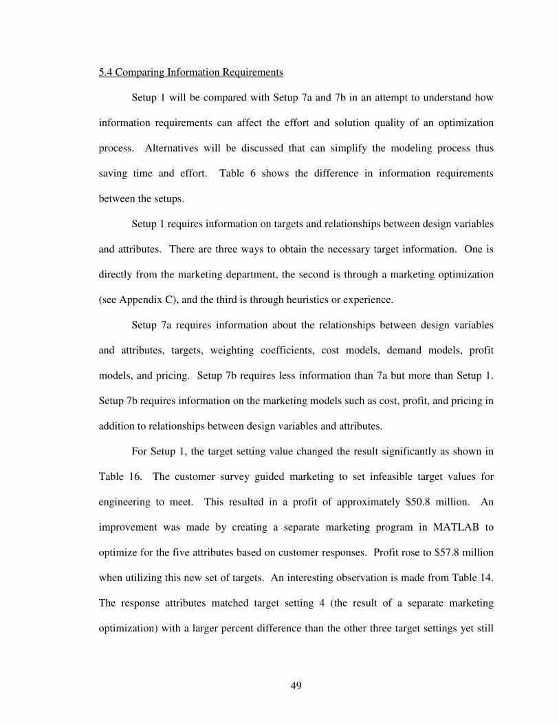
49

5.4 Comparing Information Requirements

Setup 1 will be compared with Setup 7a and 7b in an attempt to understand how

information requirements can affect the effort and solution quality of an optimization

process. Alternatives will be discussed that can simplify the modeling process thus

saving time and effort. Table 6 shows the difference in information requirements

between the setups.

Setup 1 requires information on targets and relationships between design variables

and attributes. There are three ways to obtain the necessary target information. One is

directly from the marketing department, the second is through a marketing optimization

(see Appendix C), and the third is through heuristics or experience.

Setup 7a requires information about the relationships between design variables

and attributes, targets, weighting coefficients, cost models, demand models, profit

models, and pricing. Setup 7b requires less information than 7a but more than Setup 1.

Setup 7b requires information on the marketing models such as cost, profit, and pricing in

addition to relationships between design variables and attributes.

For Setup 1, the target setting value changed the result significantly as shown in

Table 16. The customer survey guided marketing to set infeasible target values for

engineering to meet. This resulted in a profit of approximately $50.8 million. An

improvement was made by creating a separate marketing program in MATLAB to

optimize for the five attributes based on customer responses. Profit rose to $57.8 million

when utilizing this new set of targets. An interesting observation is made from Table 14.

The response attributes matched target setting 4 (the result of a separate marketing

optimization) with a larger percent difference than the other three target settings yet still

50

returned the second highest profit margin. This leads one to conclude that matching a

target setting with a small deviation is only important if the target setting is “correct” in

the first place. Information about the quality of a target setting is a good example of how

information requirements can affect the solution quality.

The $7 million improvement requires the engineer to work closely with marketing

in order to have the necessary models to perform a preliminary marketing optimization to

determine target settings. Effectively communicating marketing and engineering

disciplines has proven to cause problems [16]. In relatively simple models such as the

scale example, collaboration with marketing would allow an engineer to model a single

profit maximization problem instead of decomposing the problem into an engineering

optimization, followed by a price optimization. A better result will generally be found as

well. For example, Setup 7a returned a value of $60 million, topping Setup 1 by $3

million.

An AAO approach will result in a more profitable design simply because it

integrates more objective and enterprise level goals simultaneously. This allows for

multidisciplinary tradeoffs to be made which are otherwise unaccounted for. A downfall,

however, is that the AAO approach requires more models, more input decisions have to

be made, and the process is more computationally expensive.

Target setting and weighting coefficients have been an important topic in design

optimization for several years. A disaggregate target setting technique has been

developed and implemented by Cooper et al. [39]. Multidisciplinary design optimization

techniques have been developed as well to integrate the target setting process (product

planning) directly with design optimization (engineering analysis) [11,15,16]. The

51

importance of target setting is obvious in the bathroom scale example. When comparing

Setup 1 to Setup 7a it can be seen that with the right amount of information both setups

could potentially result in the same profit level. The two key pieces of information to do

this are the targets and the weighting coefficients. In Setup 1 (disjoint engineering

optimization) target setting 2 resulted in a profit of $64,907,000. The problem with this

solution is the simple fact that this particular target setting would likely not be known a

priori. The AAO approach has drawbacks similar to the engineering optimization. For

example, weighting coefficients play an important role in Setup 7a but have no affect on

Setup 1. If information about what weighting coefficients should be used is unknown or

difficult to determine, the AAO approach can result in a suboptimal solution. The AAO

solution with weighting coefficients, based on mathematical equivalence between the

magnitudes of profit and the target settings, resulted in $5 million less than the AAO

solution with no weighting coefficients.

Solution time is extended in the AAO approach making weighting coefficient

adjustments more manually intensive. Either case has the potential of yielding the same

result. However, adjusting target settings is more of a random process compared to

weighting coefficients. A reasonable weighting coefficient can usually be

mathematically determined by simply comparing the magnitudes of the objectives.

It appears that an engineer essentially has two choices: 1) an engineering

optimization could be performed with a significant amount of time spent finding a good

target setting to try find the best solution or 2) an AAO optimization similar to Setup 7a

could be developed with increased time spent developing and programming the models as

well as significant time spent adjusting weighting coefficients (if present) to determine

52

the optimal solution. These choices will be very dependent on the information available

at the beginning of the optimization. A designer would likely choose Setup 1 with target

setting 4 or Setup 7 if no prior knowledge of expected results or targets is known before

an optimization is performed. Setup 7b would be preferred over 7a if appropriate initial

solutions were known.

Knowledge of heuristics through experience and similar problems can

fundamentally change the way a designer models a particular problem. If targets are

known with a high degree of confidence the optimization can be simplified significantly.

On the other hand, if targets are not known or assumed with a certain confidence level

then an MDO technique may be needed to find a solution. Of course MDO techniques

are generally more difficult to model, program, and analyze. An experienced designer

will be able to assume some of these unknown values with a higher degree of accuracy

than a novice.

5.5 Effects of Decomposition

The typical product design process involves decomposing a profit-based objective

into smaller sections, usually by discipline. However, decomposing the moderately

coupled problem beyond the engineering and marketing disciplines proved to be

ineffective. Any models with moderate to high coupling will likely result in inferior

solutions and require more programming and computational effort. As shown in Table 17

Setups 2-6 required multiple MATLAB programs, more iterations and often resulted in

no solution. On the other hand Setup 1 only required 279 iterations with a profit of $50.8

million. Although there is a large difference in number of iterations, today’s computing

53

capabilities allow simple models like the ones in this experiment to be solved in less than

five minutes. Even so, the results presented here give us a good idea of the extra effort

required to formulate and solve decomposed engineering optimization problems using

different techniques. Insight into how modeling may change depending on “what we

know” can then be used to look for ways of simplifying the model and save time.

Sca

le A

nal

ysis

Res

ult

s

Des

ign

Var

iabl

es

Mar

ketin

g In

fo

Res

ult F

rom

:

x 1

x 2

x 3

x 4

x 5

x 6

x 7

x 8

x 9

x 10

x 11

x 12

x 13

x 14

Opt

imal

P

rice

($)

Mar

ket

Sha

re

Pro

fit (

$)

Set

up 1

:Tar

get 1

10.0

81.

33

10.3

41.

650.

5094

.67

0.50

6.17

1.

55

0.52

1.89

9.

58

11.7

8 10

.18

23.6

81

50.0

8%

50,7

86,0

00

Set

up 1

:Tar

get 2

5.90

5.21

1.

668.

040.

7794

.81

0.50

5.62

0.

26

0.64

1.21

9.

31

11.5

2 11

.55

26.0

26

57.2

5%

64,9

07,0

00

Set

up 1

:Tar

get 3

2.11

9.48

17

.75

0.93

8.61

94.8

50.

505.

82

0.96

0.

501.

90

9.77

11

.97

10.3

7 24

.542

53

.01%

56

,092

,000

Set

up 1

:Tar

get 4

3.30

8.62

1.

461.

720.

5195

.69

0.50

7.67

0.

35

0.55

1.90

10

.04

12.2

4 10

.64

24.8

19

53.8

7%

57,7

64,0

00

Set

up 2

36

.00

0.13

24

.00

0.13

0.13

94.5

00.

507.

44

0.50

1.

001.

00

11.9

436

.00

19.2

6 In

feas

ible

Set

up 3

36

.00

0.13

24

.00

0.13

0.13

94.5

00.

507.

44

0.50

1.

001.

00

28.5

936

.00

19.2

6 In

feas

ible

Set

up 4

8.

670.

34

23.0

00.

130.

1794

.50

2.73

4.53

1.

85

0.50

1.89

11

.94

10.9

5 10

.95

Infe

asib

le

Set

up 5

8.

670.

34

23.0

00.

130.

1794

.50

2.73

4.53

1.

85

0.50

1.89

6.

53

10.9

5 10

.95

21.0

34

38.1

2%

33,3

71,0

00

Set

up 6

17

.18

23.3

23.

5323

.39

10.5

694

.50

0.50

7.44

0.

25

1.25

1.84

9.

34

No

Fea

sibl

e S

olut

ion

Infe

asib

le

Mic

hale

k [1

6]

2.30

8.87

1.

341.

750.

4195

.70

0.50

7.44

0.

25

0.50

1.90

9.

34

11.5

4 11

.57

26.0

41

57.2

8%

64,9

90,0

00S

etup

7a:

w

= 1

05 5.

356.

23

0.45

0.49

4.07

95.5

70.

506.

60

0.35

0.

991.

81

9.40

11

.60

11.5

4 25

.820

57

.31%

60

,387

,000

Set

up 7

b: w

=1

4.78

6.84

7.

984.

514.

1095

.66

0.50

5.21

0.

51

0.63

1.70

9.

37

11.5

7 11

.59

26.0

48

57.3

0%

65,0

31,0

00

Tab

le 1

6: R

esul

ts o

f Se

ven

Scal

e O

ptim

izat

ion

Setu

ps.

55

Computation and Effort Comparison Setup Number

MATLAB Programs 1 2 3 4 5 6 7

# of Variables 14 9 9 2 2 12 15

# of Start Points 7 4 4 0 0 6 7Ave. # of Iterations/Start 39.8 18.75 18.75 0 0 20.167 461.7143

Min # of Iterations 30 12 12 0 0 18 65

Max # of Iterations 75 18 18 0 0 25 1058# of Equivalent Optimal Solutions 7 1 1 1 1 6 7

Pro

gram

1

Ave. Function Calls 677 287 287 271 1410

# of Variables 4 4 11 11 2

# of Start Points 5 5 4 4 5 Ave. # of Iterations/Start 8 8 78 78 8

Min # of Iterations 8 8 19 19 8

Max # of Iterations 8 8 235 235 8 # of Equivalent Optimal Solutions 5 5 1 1 5

Pro

gram

2

Ave. Function Calls 41 41 2750 2750 60

# of Variables 1 1

# of Start Points 7 7 Ave. # of Iterations/Start 173.5714 3.14

Min # of Iterations 3 3

Max # of Iterations 401 4 # of Equivalent Optimal Solutions 1 7

Pro

gram

3

Ave. Function Calls 3174 6

# of Variables 14 13 14 13 14 14 15

# of Start Points 7 9 16 4 11 11 7

Total # of Iterations 278.60 115.00 1330.00 312.00 333.98 161.00 3232.00

Total Function Calls 4188 1312 14000 11003 11027 1720 9875

Price $23.68 $21.03 $25.82

Market Share 50.08% 38.12% 57.30%

Tot

als/

Res

ults

Profit 50,786,000

Infeasible Infeasible Infeasible

33,371,000

Infeasible

60,387,000

Table 17: Comparing Computational Effort of Scale Analysis.

56

CHAPTER 6: ANALYSIS OF AN ELECTRIC MOTOR

This chapter continues our investigation of the tradeoffs between information

requirements and solution quality. In this chapter a common academic test problem, first

appearing in the 1970’s [37], will be used to help determine the necessary information

requirements needed to perform an optimization resulting in a quality solution. The

analysis of a universal electric motor problem originally developed by Simpson [38] will

be detailed and modified to help answer the questions arisen in the introduction.

The motor design problem is naturally a single discipline non-hierarchic problem

experiencing tight coupling among the customer attributes. Tight coupling causes

problems when attempting to decompose a design problem into subsystems because there

is no obvious way to divide the design space. Table 18 shows the degree of this coupling

through a relation matrix. The rows of Table 18 are the eight design variables. The

columns are the six constraints. An “x” indicates that the constraint is a function of the

corresponding variable. Notice power and efficiency are functions of all eight design

variables while mass and torque are functions of seven and six design variables,

respectively. As a result of the high degree of coupling, unlike the scale problem in

Chapter 5, this problem will be altered mainly through the objective function and

constraint settings. The interested reader can refer to Pan and Diaz [23] to learn about

proposed methods of dealing with decomposing tightly coupled problems into

subsystems for sequential optimization.

A marketing discipline will be added to the analysis to increase the scope of the

overall problem. This will help us understand the difference in information flow between

multidisciplinary problems and single discipline problems. The cost models used in this

57

experiment are taken from Wassenaar and Chen [30] and integrated into a simplified

discrete choice analysis model to determine demand and profits as a function of design

parameters.

Relation Matrix: Constraints vs. Design Variables

Constraints

DV H ro > ts Power (W) η Mass (kg)Torque (Nm)

Nc x x x x x Ns x x x x Arw x x x Asw x x x ro x x x x x x ts x x x x x x I x x x x

L x x x x

Table 18: Relation Matrix for the Universal Electric Motor.

6.1 Original Model Formulation

The optimization model for a universal electric motor problem includes nine

design variables [x1, …, x9], five customer attributes [z1, …, z5], twenty-three

intermediate engineering attribute calculations, five constraints, and five fixed

engineering parameters. The equations used in the model of the universal electric motor

problem will be mentioned here, however, the reader should reference Simpson [37] for

the derivations of equations and other background information on universal electric

motors. The nomenclature and equations for the design variables, fixed model

parameters, customer attributes, and constraints are listed below.

Design Variables

Nc: Number of turns of wire on the armature Ns: Number of turns of wire on the stator, per pole Aaw: Cross sectional area of armature wire [mm2]

58

Asw: Cross sectional area of stator wire [mm2] ro: Outer radius of the stator [m] ts: Thickness of the stator [m] I: Electric current [Amperes] L: Stack length [m] P: Price [$]

Engineering Attributes

H: Magnetizing intensity [Ampere turns/m] => c c r gH=N I/(l +l +2l )

lc: Mean path length within the stator [m] => c o sl (2r +t )/2π=

lr: Diameter of armature [m] => r o s gl =2(r -t -l )

Pin: Input power [W] => in tP =V I

Pout: Power losses due to copper and brushes [W] => 2out a sP =I (R +R )+2I

law: Armature wire length [m] => aw o s g cl =2L+4(r -t -l )N

lsw: Stator wire length [m] => sw st o s sl =p (2L+4(r -t ))N

Ra: Armature wire resistance [Ohm] => a aw awR l /Aρ=

Rs: Stator wire resistance [Ohm] => s sw swR l /Aρ=

Mw: Mass of windings [kg] => w aw aw sw swM =(l A +l A ) copperρ

Ms: Mass of stator [kg] => 2 2s o o sM L(r -(r -t ) ) steelπ ρ=

Ma: Mass of armature [kg] => 2a o s gM L(r -t -l ) steelπ ρ=

K: Motor constant [dimensionless] => cK=N /π

ℑ: Magneto magnetic force [A turns] => sN Iℑ =

ℜ: Total reluctance of the magnetic circuit [A turns/Wb] => 2s a gℜ = ℜ + ℜ + ℜ

ℜs: Reluctance of stator [A turns/Wb] => c sl /(2 A )s steel oµ µℜ =

ℜa: Reluctance of armature [A turns/Wb] => r al /( A )a steel oµ µℜ =

ℜg: Reluctance of one air gap [A turns/Wb] => g gl /( A )g oµℜ =

As: Cross sectional area of stator [m2] => s sA =t L

Aa: Cross sectional area of armature [m2] => a rA =l L

Ag: Cross sectional area of air gap [m2] => g gA =l L

µsteel: Relative permeability of steel [dimensionless] =>

20.2279 52.411 3115.8 220

11633.5 1486.33ln( ) 220 1000

1000 1000

steel

steel

steel

H H H

H H

H

µ

µ

µ

= − + + ≤

= − < ≤

= >

ϕ: Magnetic flux [Wb] => /ϕ = ℑ ℜ

59

Fixed Engineering Parameters

lg: Length of air gap = 7.0 x 10-4 [m] Vt: Terminal voltage = 115 [V] ρ: Resistivity of copper = 1.69 x 10-8 [Ohms•m] µo: Permeability of free space = 4π x 10-7 [H/m] pst: Number of stator poles = 2

Customer Attributes

T: Torque [Nm] => T=K Iϕ

P: Power [W] => in outP=P -P

η: Efficiency [%] => inP/Pη =

M: Mass [kg] => w s aM=M +M +M

B: Operating Time = η

Constraints and Bounds

H ≤ 5000 [A turns/m] ro > ts

P = 300 [W] T = {0.05, 0.10, 0.125, 0.3, 0.5} [Nm] η ≥ 0.15 M ≤ 2.0 [kg]

Bounds on Design Variables Nc Ns Aaw Asw ro ts I L

LB 100 1 0.01 0.01 0.01 0.0005 0.1 0.01 UB 1500 500 1.0 1.0 0.1 0.01 6 0.2 Unit turns turns mm2 mm2 m m A m

Table 19: Bounds on Design Variables.

Marketing Related Models

The profit model is a basic model that incorporates demand (q), price (p), and

several design dependent costs. The cost model equations used for this analysis were

originally derived in Wassenaar and Chen [30]. The following analysis simplifies the

cost model slightly and creates a different discrete choice analysis model to predict

60

demand. The profit model used in the analysis of the universal electric motor is shown in

equation 6.1.

Cpq −=Π )( (6.1)

where C is a summation of cost functions as follows:

( )( )

( )( )2

$500,000

30 / 70

50 500,000 /1000

c c c cap

c

c w copper s r steel

c c

cap

C D M L C

D

M q M P M M P

L M

C q

= + + +

=

= + +

=

= −

The design cost Dc is assumed to be fixed at $500,000 while the material cost Mc, labor

cost Lc, and capacity cost Ccap varies with demand and engineering attributes.

The demand model was developed using discrete choice analysis (DCA) and

synthetic spline functions for customer preference. The total demand is population size

multiplied by the probability that a consumer will select a particular design (i.e. estimated

market share). Equation 6.2 shows the common DCA equation developed in [34, 35].

( )

1

1

1

1

( )

v v

K

k Kkk

q sP se e

s population size

z pν

−

−

=

⎡ ⎤= = +⎣ ⎦=

= Ψ + Ψ∑

(6.2)

The attraction value “ν” is simply the summation of the beta values calculated from the

spline functions for each attribute value and price. The spline functions are shown in

Appendix B.

61

6.2 Optimization Setups

Five main setups are considered for the analysis on optimizing a universal electric

motor. The first four setups include only the engineering discipline. An attribute-based

objective function will be used to determine an optimal motor design. The results are then

entered into a marketing optimization to determine price and profit so that a comparison

can be made between the disjoint optimizations and the all-at-once (AAO) approach. The

design space is bounded by the six constraints listed above. The fifth method adds the

marketing domain and related models to create an AAO optimization. Figure 4 gives a

clearer picture of the five setups. In this example no extra constraints are applied when

marketing is added. Weighting coefficients will be studied for the multi-objective

optimizations along with various other changing parameters. Two types of weighting

coefficients are used in this example. The first is added to simply balance the difference

in magnitudes between the objectives in the multi-objective case. The second set of

weights adds preference to one or more attributes within the l2 deviation segment of the

objective function. Weighting coefficients will be discussed within each setup when

relevant.

62

Figure 4: Breakdown of Setups for Motor Analyses

Setup Class Objective Information Requirments

Output

1 S-E-AA Min M - η DV Attributes x1-x8

2 S-E-AA Min M-η+ Dev. DV Attributes x1-x8

3 S-E-A Min M DV Attributes x1-x8

4 S-E-A Min -η DV Attributes x1-x8

5a S-EP-Π Min –Π + Dev. DV Attributes, Attr. Demand Targets, Weights, Price Demand

Cost & Profit Models x1-x8, price

5b S-EP-AΠ Min -ΠDV Attributes, Attr. Demand

Price Demand, Cost & Profit Models x1-x8, price

Table 20: Details of the Six Motor Setups.

The table above gives a breakdown of the six different setups used in the analysis

of a universal electric motor. All six setups require information regarding the

relationship between the design variables and attributes. Similar to the scale example, the

major differences in information requirements can be found in Setups 5a and 5b. Setup

5a requires six more major pieces of information compared to Setups 1-4. This includes

Setup Breakdown

Engineering Engineering

+ Marketing

Setup 1Min f = M-η P = 300 W

T = 0.05-0.5 Nm

Setup 2Min f =

M-η+||T-Z||2

Setup 3Min f = M P = 300 W

T = 0.05-0.5 Nm

Setup 4Min f = -η P = 300 W

T = 0.05-0.50 Nm

Setup 5Min f =

-Π+||T-Z||2

63

information on target settings, weights, pricing, cost models, profit models, and

relationships between attributes and demand. Setup 5b is slightly less involved because

information on targets and weights is not necessary. All six setups output values for the

eight engineering design variables but Setups 5a and 5b also include a price output. The

objective functions will be discussed in more detail later in this section.

The five initial solutions used for all five of the setups are shown in Table 21.

The first initial solution is the lower bound on all eight design variables. The second

initial solution is the upper bound on all eight design variables. Initial solution three is

the median of the range for each of the eight design variables. Initial solutions four and

five were arbitrarily chosen with values for ro and ts extending beyond the actual range

for each respective design variable. Finally, the sixth and seventh initial solutions are the

75% and 25% values among the range for each design variable, respectively.

Initial Solutions DV 1 2 3 4 5 6 7

Nc 100 1500 800 1062 730 1150 450 Ns 1 500 250.5 54 45 375.25 125.75 Aaw 0.01 1 0.505 0.241 0.203 0.7525 0.2575 Asw 0.01 1 0.505 0.376 0.205 0.7525 0.2575 ro 0.01 0.1 0.055 2.59 3.62 0.0775 0.0325 ts 0.0005 0.015 0.00775 6.66 9.69 0.011375 0.004125 I 0.1 6 3.05 4.29 3.65 4.525 1.575 L 0.01 0.2 0.105 2.6 0.998 0.1525 0.0575

Table 21: Initial solutions for Universal Electric Motor Optimizations.

Five different torque requirements will be used to optimize five different motor

designs. Each motor design can be thought of as an individual optimization with no

coupling between the other motors. If there were a link between the five torque settings

then the optimization could become a product family, which is performed in Simpson et

64

al. [37]. Benchmark motor designs shown in Table 22 will be used to compare the

correctness of the optimization results.

Benchmark Motor Designs

MotorNc

(turns)Ns

(turns)Aaw

(mm2)Asw

(mm2)ro

(cm)ts

(mm) I

(A) L

(cm) T

(Nm) P

(W)η

(%) M

(kg)

1 730 45 0.203 0.205 3.62 9.69 3.65 0.998 0.05 300 71.4 0.5 2 750 76 0.186 0.203 3.31 11.77 3.73 1.28 0.1 300 70.6 0.5 3 760 89 0.19 0.203 3.12 11.2 3.73 1.41 0.125 300 70 0.5 4 1030 73 0.253 0.23 2.44 6.35 4.19 2.74 0.3 300 62.2 0.7125 1087 72 0.284 0.247 2.71 7.15 4.71 3.16 0.5 300 55.3 0.985

Table 22: Benchmark Motor Designs [37].

6.2.1 Setup 1: Multi-objective Tradeoff between Mass and Efficiency.

This setup is based off examples found in [30, 36, 37]. The overall objective is

to minimize mass while maximizing efficiency. Power and torque are set as equality

constraints to match the company decided necessary requirements. The equality

constraints make all the initial solutions infeasible initially since none of the seven initial

solutions meet the exact torque and power requirements. The objective function used for

all five motors designs in Setup 1 is shown in equation 6.3. No weighting coefficients are

used during this optimization because the magnitude of mass and efficiency are

comparable. Mass ranges from 0 to 2.0 kilograms while efficiency ranges from 0 to 100

percent (0 – 1.0).

min f M η= − (6.3)

Once the engineering optimization is complete the solutions are evaluated in the

following way: They are entered as fixed values into a secondary price optimization to

determine the best price and maximum achievable profit (see Appendix C).

65

6.2.2 Setup 2: Multi-objective Tradeoff between Mass and Efficiency

Setup 2 is a modification to Setup 1 that will provide information on the effect

that target settings have on an optimization solver. For this setup the equality constraints

for torque and power are replaced with target settings in the objective function. Using the

same initial solutions, an attempt to meet the torque and power requirements through

target settings will be made to study how the optimizer reacts and see if a quality solution

can be found. This can be useful in a situation where the equality constraints cannot be

met but a satisfactory solution within a specified tolerance may be found. Removing the

equality constraints allows some of the initial solutions to be feasible because the stiff

requirements are initially removed. Equation 6.4 shows the objective function used in

Setup 2. The l2 norm of the difference between target and response values for torque and

power are added to the original multi-objective function in Setup 1.

2min ( )f M w T Zη= − + − (6.4)




It is important to have weights on the deviations of torque and power since torque

ranges from 0.05 – 0.5 Nm and power is fixed at 300. For example, with a torque

requirement of 0.05 Nm the vector w is set to [600 1]. Element by element matrix

multiplication takes the difference in torque and multiplies it by 600 while the difference

in power is multiplied by one. This balances the difference in magnitude between torque

and power. These weights are adjusted to study how different values change the result.

66

6.2.3 Setup 3: Minimizing Mass

Setup 3 simplifies the objective function be removing the efficiency objective. It

is expected that minimizing mass using equality constraints for torque and power would

return a solution quicker than the previous two setups simply because it is single

objective. Equation 6.5 shows the simplified objective function.

min f M= (6.5)




6.2.4 Setup 4: Maximizing Efficiency

Setup 4 is again a single objective optimization to maximize efficiency. Torque

and power are set as equality constraints as in Setup 1. Setups 3 and 4 will allow a

comparison to be made between the difference in solution quality when a problem that

logically should be solved using a multi-objective function is solved using each objective

individually. Equation 6.6 shows the objective function used for this setup.

min f η= − (6.6)




67

6.2.5 Setup 5: All-at-Once

This setup is important for several reasons. Advantages or disadvantages of a joint

optimization can be studied using an AAO approach and comparing it to the previous

disjoint optimization setups. Also, although the all-at-once approach is limited to small

multi-disciplinary problems, important information about the knowledge required to

perform such an optimization can be studied through simple examples. AAO increases

scope and complexity by considering customer preference directly in the optimization.

The AAO optimization of a universal electric motor is tried using both equality

constraints and target settings to meet torque and power requirements. Target settings in

the AAO approach are different from other multi-disciplinary optimization techniques

because no coordination among disciplines is required. It is common for various

decomposition techniques in multi-disciplinary optimization to use target settings to

coordinate disciplines and guide them toward the same solution. The objective functions

for these setups are shown in equation 6.7. The first equation of 6.7 has been used for the

MDO technique known as analytical target cascading [16, 17]. The second equation of

6.7 is a common objective function for decision-based design (DBD). Typically DBD

optimizations are profit-based single objective optimizations.

1 2 25 : min ( )

5 : min

Setup a f w w T Z

Setup b f

= −Π + −

= −Π (6.7)

6.3 Results of Universal Electric Motor Analysis

The results will be displayed and compared in several different tables. First the

result of each setup with the lowest objective function value (i.e. “best”) for each torque

requirement will be displayed. This will allow easy comparison with the benchmark

68

motor designs shown in Table 22. Then Section 6.4 will compare the information

requirements between several setups, Section 6.5 will discuss how “rules of thumb” can

affect the selection of an objective function, and finally Section 6.6 will analyze how the

use of target settings in the objective function affects the solution.

6.3.1 Results of each Setup

Best Result: Setup 1 0.05 Nm 0.10 Nm 0.125 Nm 0.3 Nm 0.5 Nm

Nc (turns) 698.3939 873.8862 931.4766 1062.5550 1161.1770Ns (turns) 57.5732 58.0332 56.8460 40.2552 46.3483Aaw (mm2) 0.2087 0.2087 0.2087 0.2155 0.2737Asw (mm2) 0.2087 0.2087 0.2087 0.2156 0.2737ro (m) 0.0161 0.0184 0.0191 0.0214 0.0249ts (m) 0.0026 0.0031 0.0033 0.0037 0.0047I (A) 3.1967 3.5952 3.8081 6.0000 6.0000L (m) 0.0196 0.0219 0.0226 0.0246 0.0287Efficiency 0.8161 0.7256 0.6850 0.4348 0.4348Mass (kg) 0.2553 0.3614 0.3992 0.5215 0.8352Power (W) 300.0000 300.0000 300.0000 299.9999 299.9999Profit ($) 2,691,980 2,316,635 2,169,453 1,492,425 894,234

Table 23: Results of Multi-Objective Optimization.

It can be seen from Table 23 that the torque and power requirements have been

met for each of the five motor designs. As expected the mass increases and efficiency

decreases as the torque increases from 0.05 through 0.5 Nm. The efficiency is

dramatically less for the larger motors because a large current is necessary to meet the

power constraint.

69


Nc (turns) 867.2270 732.7830 1023.9600 1059.6100 1061.7800Ns (turns) 38.6611 58.4106 34.2572 104.0420 101.5650Aaw (mm2) 0.3072 0.5523 0.2752 0.3404 0.3815Asw (mm2) 0.6949 0.3528 0.4971 0.3339 0.6086ro (m) 0.0198 0.0256 0.0304 0.0393 0.0336ts (m) 0.0051 0.0045 0.0037 0.0039 0.0056I (A) 3.0708 2.9592 4.0591 4.5190 3.7542L (m) 0.0224 0.0290 0.0217 0.0121 0.0290Efficiency 0.8495 0.8815 0.6427 0.5773 0.6949Mass (kg) 0.4935 1.0075 0.8936 1.0748 1.5737Power (W) 300.0000 300.0000 300.0000 300.0000 300.0000Profit ($) 2,249,784 1,298,245 1,095,600 610,753 -36,241

Table 24: Results of MO Optimization with Target Settings.

Similar to Setup 1 the mass increases more dramatically in Setup 2 than

efficiency. Torque and power requirements have been met for all five motor designs with

similar results to Setup 1. Apparently mass was not given as much importance as

efficiency because both are higher in Setup 2. No weights were given to either because

their magnitudes are similar so there is no clear explanation for why there is a large

difference in mass from Setup 1. Efficiency seems to improve greatly as torque

increases, however, mass also increases greatly.


Nc (turns) 732.3850 880.4442 908.7270 1056.4000 1159.3206Ns (turns) 24.8018 29.7585 31.7158 40.3948 46.3208Aaw (mm2) 0.0907 0.1294 0.1429 0.2150 0.2734Asw (mm2) 0.0908 0.1291 0.1429 0.2148 0.2751ro (m) 0.0127 0.0155 0.0166 0.0214 0.0249ts (m) 0.0017 0.0023 0.0026 0.0037 0.0047I (A) 6.0000 6.0000 6.0000 6.0000 6.0000L (m) 0.0152 0.0177 0.0189 0.0247 0.0288Efficiency 0.4348 0.4348 0.4348 0.4348 0.4348Mass (kg) 0.1012 0.1902 0.2334 0.5215 0.8352Power (W) 299.9998 299.9999 299.9999 299.9999 299.9999Profit ($) 2,314,632 2,136,571 2,052,662 1,492,400 899,324

Table 25: Results of Single Objective Optimization to Minimize Mass.

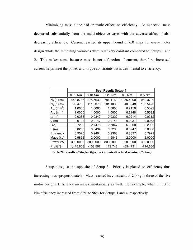
70

Minimizing mass alone had dramatic effects on efficiency. As expected, mass

decreased substantially from the multi-objective cases with the adverse affect of also

decreasing efficiency. Current reached its upper bound of 6.0 amps for every motor

design while the remaining variables were relatively constant compared to Setups 1 and

2. This makes sense because mass is not a function of current, therefore, increased

current helps meet the power and torque constraints but is detrimental to efficiency.


Nc (turns) 443.8787 275.5630 781.1160 1056.4000 1062.3700Ns (turns) 92.4786 111.2370 101.1030 40.3948 103.5470Aaw (mm2) 1.0000 1.0000 1.0000 0.2150 0.5592Asw (mm2) 1.0000 1.0000 1.0000 0.2148 0.5592ro (m) 0.0288 0.0347 0.0322 0.0214 0.0312ts (m) 0.0133 0.0147 0.0148 0.0037 0.0068I (A) 2.7260 2.7478 2.7847 6.0000 3.2902L (m) 0.0208 0.0434 0.0233 0.0247 0.0388Efficiency 0.9570 0.9494 0.9368 0.8897 0.7929Mass (kg) 0.9892 2.0000 1.5843 2.0000 2.0000Power (W) 300.0000 300.0000 300.0000 300.0000 300.0000Profit ($) 1,445,608 -158,592 179,748 -654,731 -714,666

Table 26: Results of Single Objective Optimization to Maximize Efficiency.

Setup 4 is just the opposite of Setup 3. Priority is placed on efficiency thus

increasing mass proportionately. Mass reached its constraint of 2.0 kg in three of the five

motor designs. Efficiency increases substantially as well. For example, when T = 0.05

Nm efficiency increased from 82% to 96% for Setups 1 and 4, respectively.

71


Nc (turns) 770.9107 638.4883 749.7149 928.3510 1013.6319Ns (turns) 53.0176 81.3443 65.7928 79.5408 79.0881Aaw (mm2) 0.2573 0.3184 0.3167 0.2637 0.2993Asw (mm2) 0.2362 0.2927 0.3046 0.2712 0.4038ro (m) 0.0145 0.0224 0.0188 0.0289 0.0311ts (m) 0.0025 0.0041 0.0033 0.0042 0.0042I (A) 3.1068 3.0952 3.2112 4.2013 4.5787L (m) 0.0225 0.0244 0.0348 0.0231 0.0287Price ($) 7.1279 6.7501 6.5867 5.6217 4.9559Efficiency 0.8397 0.8428 0.8124 0.6209 0.5697Mass (kg) 0.2898 0.5565 0.6039 0.8253 1.1926Power (W) 300.0 300.0 300.0 300.0 300.0Profit ($) 2,641,216 2,159,373 1,986,651 1,274,171 507,865

Table 27: Results of AAO Optimization

The results shown in Table 27 are from Setup 5a. Again the targets for power and torque

were met for all five motor designs. Notice that efficiency does not decrease as quickly

as in Setup 1, however, mass increases faster in Setup 5 than Setup 1.

Notice the large deviation in profit between the 0.05 Nm motor and the 0.5 Nm

motor. This is believed to have occurred because of the simplicity in the spline functions

used to estimate customer demand. Mass plays a large role in determining customer

preference and a larger motor will obviously have a larger mass automatically making it

less appealing, even if the torque is higher. Realistically there should be separate demand

models for each motor size to more accurately represent the market segments.

6.3.2 Comparing Five Setups for T = {0.05, 0.10, 0.125, 0.30, 0.50} Nm

Table 28 displays the results of all five setups for motor design 1 (i.e. T = 0.05

Nm). Information from the optimization such as number of iterations, number of

function calls, number of infeasible solutions, active constraints (ineqlin and ineqnonlin),

and which initial solution returned the optimal design are displayed as well.

72

Each motor design from the first four setups was entered into a marketing

optimization to determine price and maximum profit. This gives a basis for comparing

the engineering optimizations with the AAO approach. It can be seen that the best result

is from Setup 1. Setup 5b returned the next best solution based on profit margin alone.

Table 29 displays the results of motor design 2 (T = 0.10 Nm). Similar trends can

be seen in these results as in Table 28. The main difference in this motor design is seen

in Setup 4. The efficiency optimization results in a negative profit even though it has a

value of almost 95%. Because mass is sacrificed at the expense of efficiency and the

demand and cost models are both functions of mass, a small increase in mass will have a

large role in profit margin. Efficiency is only included in the demand function and

therefore has less importance.

Table 30 displays the results of motor design 3 (T = 0.125 Nm). Similar trends to

the first two motors are seen here except in this case the single objective optimization to

minimize mass results in a higher profit than three of the other setups.

The results of motor designs 4 and 5 are displayed in Tables 31 and 32,

respectively. Again similar trends can be seen in all the optimizations. As the torque

requirement increases the single objective mass optimization becomes the more preferred

method. Tables 28 – 32 are at the end of Chapter 6.

6.4 Comparing Information Requirements

The universal electric motor example is a better example at demonstrating how

information requirements affect the solution effort and quality when using different

modeling approaches. Setup 1 will be compared to Setup 5b and Setup 2 will be

73

compared to Setup 5a to understand the importance of information requirements on the

solution quality. Table 20 provides a detailed breakdown of the information

requirements involved in the different setups. Setup 1 is most similar to Setup 5b

because both use equality constraints to meet torque and power requirements. Setup 2 is

most similar to Setup 5a because both utilize a target deviation term in the objective

function to meet torque and power requirements.

Both Setups 1 and 5b require information about how attributes are related to

design variables, however, Setup 5b also requires information about the relationships

between attributes and demand, price and demand, as well as information on cost models,

and profit models. This is a significant amount of information to gather prior to creating

an optimization model and there is no clear way to quantify this amount or the effort

required to gather it. The most interesting result is that Setup 5b does not find a solution

for any starting point. All the effort that went into developing the extra models would

have been a waste of time. Setup 1 finds the highest profit of all the setups, so in this

example developing marketing models is a waste of time anyway.

The information requirements between Setups 2 and 5a are more involved than

for Setups 1 and 5b. Setup 2 requires information about the relationships between design

variables and attributes as well as target settings. Setup 5b, on the other hand, requires

information about the relationships between the design variables, attributes, price and

demand models. In addition cost models, profit models, weighting coefficients, and

targets have to be considered. The advantage of performing the necessary work to

develop all of these models is that Setup 5a returns $391,433 more than Setup 2.

Determining if the extra effort and time it took to develop such models is worth close to

74

$400,000 is a difficult task. Setup 5b required user adjustments within MATLAB to find

a solution.

Similar issues to those of the scale example also arise with the AAO approaches

in this example problem. For example, adding spline functions from discrete choice

analysis for customer preference required additional statements in the computer program

to help keep the optimizer within the customer attribute bounds. The additional

statements were arbitrarily chosen and it is not known if the optimization algorithm is

sensitive to it.

Weighting coefficients for Setups 2 and 5a played an important role as well. If

the norm of the deviation (w1 in equation 6.7) was not multiplied by a value of 100,000 or

higher no solution was found. However, a lower profit resulted for a value higher than

100,000. Similarly, the weights placed on the target attributes altered the solution

significantly. If a coefficient less than 125 was placed on the torque deviation the

optimizer found no solution. I do not see any significance in this value since, for

example, one might expect the weight on torque for T = 0.05 Nm to be 6000 in order to

balance with power. An optimization was run using Setup 2 with w from equation 6.4 as

a variable because of the large range of possible weights. When started at 6000 the

solution returned an optimal value of 5839. A solution was found in the same number of

iterations as the case when w was fixed and also improved mass by 13.07% while

decreasing efficiency by only 1.53%. It is determined through trial and error that the

initial guess for the weight must be at least 160 or no feasible solution is found. When

the weight is started at 160 the optimal result is 242 but the solution is suboptimal, based

on profit alone, compared to the result when w is 5839.

75

6.5 Using Rules of Thumb in Choosing an Objective Function

Setup 1 will be compared to Setups 3 and 4 to see how rules of thumb, usually

obtained through experience and sometimes called heuristics, could affect how an

objective function is chosen along with the possible solutions that can be obtained. All

three setups use equality constraints. The only difference between them is seen in the

objective function formulation.

The universal electric motor design is a tightly coupled model with many

intermediate functions. The objective functions in this example were fundamentally

different from those in the scale example because target settings were not required. The

original goals were to minimize mass and maximize efficiency with an enterprise goal to

maximize profit. The objective function type again played an important role in

maximizing profit. There appears to be a sensitive relation between the objective

function used and the demand model. Comparing Tables 28, 30, and 31 shows how this

relation affects the result. As the motor torque requirement increases from 0.05 Nm to

0.30 Nm, the single objective mass optimization (Setup 3) continuously returns higher

profits relative to Setups 1 and 4. This probably occurs because of the way the cost

modeling and customer demand modeling was carried out. The only customer attribute

that the cost depended on was mass so it makes sense that a lighter motor is going to

yield higher profits. Marketing information is not always readily available or accurate so

target setting is still a difficult task.

Comparing results from Setups 1, 3, and 4 used in the motor design analyses

brings to light another example of how a designer’s experience and knowledge base can

affect the way an optimization problem is formulated. The cost models used in the

76

analysis are functions of only one out of four attributes. Mass appears in two of the four

equations used to model cost. As a result cost is very sensitive to mass. For larger

motors such as when T = 0.50 Nm the profit will automatically be less simply because

the motor is heavier.

This shows the importance of cost and demand modeling but it also gives a solid

relationship relative to the qualitative nature of the problem. If an engineer is aware of

this relationship through previous examples or past experience the model may be

simplified. Minimizing mass solely results in a higher profit for the larger motors than

any of the other four objective functions. Maximizing efficiency, on the other hand,

returns very poor solutions based on profit. Although customers desire high efficiency,

choosing to maximize efficiency with no consideration for mass would be a bad rule of

thumb to follow. Since single objective functions are generally simpler to formulate and

solve, especially in single discipline optimizations, an appropriate rule of thumb could

reduce the effort needed to find an optimal result. Essentially an optimization to

maximize profit could be performed without actually solving a profit maximization

problem.

6.6 Target Matching in the Objective

Target matching in the objective function played a large role in reducing the

affects of initial solutions. For example, take motor designs 2-5 (T = 0.1, 0.125, 0.3, and

0.5 Nm). The multi-objective optimization of Setup 1 experienced at least one infeasible

solution for the set of initial solutions mentioned in Table 21. Setup 1 uses equality

constraints to meet torque and power requirements. Setup 2, which adds a target

77

matching term to the objective function, finds a solution for every starting point of every

motor design.

The tradeoff is seen when the results of Setups 1 and 2 are entered into a price

optimization to determine profit. Setup 2 returns a profit margin that is $442,196 less

than Setup 1. This seems like a huge tradeoff, but there may be design problems that

cannot find a feasible solution when equality constraints are used. Target matching may

be an alternative method to help get a solution. Of course one can assume the result is

not the global optima, but it’s better than not finding any solutions.

This exact situation can be seen when Setups 5a and 5b are compared. Setup 5b

is a profit maximization problem utilizing equality constraints on power and torque.

When this model is solved no solution is found for any of the starting points. The

optimization terminates after just a few iterations claiming no feasible solution can be

found. In an attempt to find a solution, Setup 5a was used. This setup adds a target

matching objective to the profit objective. When this model is solved a solution is found

for every starting point.

Since it would not be known if the optimizer will find a solution before a model is

built and solved, a comparison cannot be made between the advantages of solving Setup

1 versus Setup 5a. However, it is useful to know that a simple modification to the

objective function and constraints could improve the possibility of finding a solution.

Co

mp

aris

on

of

Res

ult

s fo

r M

oto

r D

esig

n 1

(T

= 0

.05

Nm

) F

orm

ula

tio

ns

Des

ign

Var

iab

les

No

men

clat

ure

M

ult

i-o

bje

ctiv

e M

O w

ith

Tar

get

sM

ass

Eff

icie

ncy

A

AO

# w

ire tu

rns

on a

rmat

ure

Nc

(tu

rns)

69

8.39

1686

7.22

7073

2.38

5044

3.87

8777

0.91

07#

wire

turn

s on

sta

tor

Ns

(tu

rns)

57

.573

238

.661

124

.801

892

.478

653

.017

6x-

sect

. are

a of

arm

. Wire

Aaw

(m

m2 )

0.20

870.

3072

0.09

071.

0000

0.25

73x-

sect

. are

a of

sta

tor

wire

Asw

(m

m2 )

0.20

870.

6949

0.09

081.

0000

0.23

62st

ator

rad

ius

r o (

m)

0.01

610.

0198

0.01

270.

0288

0.01

45st

ator

thic

knes

st s

(m

) 0.

0026

0.00

510.

0017

0.01

330.

0025

curr

ent

I (A

) 3.

1967

3.07

086.

0000

2.72

603.

1068

stac

k le

ngth

L (

m)

0.01

960.

0224

0.01

520.

0208

0.02

25P

ow

er (

W)

300.

0000

300.

0000

299.

9998

300.

0000

300.

0000

To

rqu

e (N

m)

0.05

000.

0500

0.05

000.

0500

0.05

00E

ffic

ien

cy

0.81

610.

8495

0.43

480.

9570

0.83

97M

ass

(kg

) 0.

2553

0.49

350.

1012

0.98

920.

2898

Pri

ce (

$)

7.12

79

Cus

tom

er A

ttrib

utes

Pro

fit

($)

2,64

1,21

7O

bj.

Fu

nct

. -0

.560

7-0

.356

00.

1012

-0.9

570

-264

1195

.333

Lo

wer

Up

per

7

3,4

in

eqlin

ineq

no

nlin

1

11

#

iter

atio

ns

9956

227

2111

1#

fun

ctio

n c

alls

921

824

2215

20

1 15

00#

infe

asib

le s

ln.

00

00

0

Pro

pert

ies

of O

ptim

izat

ion

Init

ial s

olu

tio

n #

4,5

25

71

Pri

ce (

$)

7.08

606.

8699

6.03

496.

5400

Pric

e O

ptim

izat

ion

Pro

pert

ies

Pro

fit

($)

2,69

1,98

02,

249,

784

2,31

4,63

21,

445,

608

Tab

le 2

8: C

ompa

riso

n of

Fiv

e Se

tups

on

Mot

or D

esig

n 1

Co

mp

aris

on

of

Res

ult

s fo

r M

oto

r D

esig

n 2

(T

= 0

.10

Nm

) F

orm

ula

tio

ns

Des

ign

Var

iab

les

No

men

clat

ure

M

ult

i-o

bje

ctiv

e M

O w

ith

Tar

get

s M

ass

Eff

icie

ncy

A

AO

# w

ire tu

rns

on a

rmat

ure

Nc

(tu

rns)

87

3.92

8773

2.78

3088

0.44

4227

5.56

3063

8.48

83#

wire

turn

s on

sta

tor

Ns

(tu

rns)

58

.033

458

.410

629

.758

511

1.23

7081

.344

3x-

sect

. are

a of

arm

. Wire

Aaw

(m

m2 )

0.20

870.

5523

0.12

941.

0000

0.31

84x-

sect

. are

a of

sta

tor

wire

Asw

(m

m2 )

0.20

870.

3528

0.12

911.

0000

0.29

27st

ator

rad

ius

r o (

m)

0.01

840.

0256

0.01

550.

0347

0.02

24st

ator

thic

knes

st s

(m

) 0.

0031

0.00

450.

0023

0.01

470.

0041

curr

ent

I (A

) 3.

5952

2.95

926.

0000

2.74

783.

0952

stac

k le

ngth

L (

m)

0.02

190.

0290

0.01

770.

0434

0.02

44P

ow

er (

W)

300.

0000

300.

0000

299.

9999

300.

0000

300.

0000

To

rqu

e (N

m)

0.10

000.

1000

0.10

000.

1000

0.10

00E

ffic

ien

cy

0.72

560.

8815

0.43

480.

9494

0.84

28M

ass

(kg

) 0.

3614

1.00

750.

1902

2.00

000.

5565

Pri

ce (

$)

6.75

01

Attr

ibut

es

Pro

fit

($)

2,15

9,37

3O

bj.

Fu

nct

. -0

.364

20.

1260

0.19

02-0

.949

4-2

1593

71.4

532

low

er

u

pp

er

73,

4

ineq

lin

in

eqn

on

lin

1

# it

erat

ion

s 10

912

133

754

131

# fu

nct

ion

cal

ls

1034

16

35

3455

51

4 15

92#

infe

asib

le s

ln.

10

10

0

Pro

pert

ies

of O

ptim

izat

ion

Init

ial s

olu

tio

n #

5,

73

72

7

Pri

ce (

$)

6.63

696.

2594

5.91

085.

0309

Pric

e O

ptim

izat

ion

Pro

pert

ies

Pro

fit

($)

2,31

6,63

51,

298,

245

2,13

6,57

1-1

58,5

92

Tab

le 2

9: C

ompa

riso

n of

Fiv

e Se

tups

on

Mot

or D

esig

n 2

Co

mp

aris

on

of

Res

ult

s fo

r M

oto

r D

esig

n 3

(T

= 0

.125

Nm

) F

orm

ula

tio

ns

Des

ign

Var

iab

les

No

men

cl.

Mu

lti-

ob

ject

ive

MO

wit

h T

arg

ets

Mas

s E

ffic

ien

cy

AA

O#

wire

turn

s on

arm

atur

eN

c (t

urn

s)

931.

4766

736.

8520

908.

7270

781.

1160

749.

7149

# w

ire tu

rns

on s

tato

rN

s (t

urn

s)

56.8

460

61.9

368

31.7

158

101.

1030

65.7

928

x-se

ct. a

rea

of a

rm. W

ireA

aw (

mm

2 ) 0.

2087

0.47

070.

1429

1.00

000.

3167

x-se

ct. a

rea

of s

tato

r w

ireA

sw (

mm

2 ) 0.

2087

0.52

770.

1429

1.00

000.

3046

stat

or r

adiu

sr o

(m

) 0.

0191

0.02

850.

0166

0.03

220.

0188

stat

or th

ickn

ess

t s (

m)

0.00

330.

0053

0.00

260.

0148

0.00

33cu

rren

tI (

A)

3.80

813.

0242

6.00

002.

7847

3.21

12st

ack

leng

thL

(m

) 0.

0226

0.02

980.

0189

0.02

330.

0348

Po

wer

(W

) 30

0.00

0030

0.00

0029

9.99

9930

0.00

0030

0.00

00T

orq

ue

(Nm

) 0.

1250

0.12

500.

1250

0.12

500.

1250

Eff

icie

ncy

0.

6850

0.86

260.

4348

0.93

680.

8124

Mas

s (k

g)

0.39

921.

1261

0.23

341.

5843

0.60

39P

rice

($)

6.

5867

Attr

ibut

es

Pro

fit

($)

1,98

6,65

2O

bj.

Fu

nct

. -0

.285

80.

2634

0.23

34-0

.936

8-1

9866

45.0

986

low

er

u

pp

er

73,

4

ineq

lin

in

eqn

on

lin

11

1

# it

erat

ion

s 50

7648

929

1586

# fu

nct

ion

cal

ls

465

1076

51

04

304

3549

8#

infe

asib

le s

ln.

10

10

0

Pro

pert

ies

of O

ptim

izat

ion

Init

ial G

ues

s #

23

73

6

Pri

ce (

$)

6.44

926.

0171

5.85

015.

6728

Pric

e O

ptim

izat

ion

Pro

pert

ies

Pro

fit

($)

2,16

9,45

31,

095,

600

2,05

2,66

217

9,74

8

Tab

le 3

0: C

ompa

riso

n of

Fiv

e Se

tups

on

Mot

or D

esig

n 3

Co

mp

aris

on

of

Res

ult

s fo

r M

oto

r D

esig

n 4

(T

= 0

.3 N

m)

Fo

rmu

lati

on

s D

esig

n V

aria

ble

s N

om

encl

atu

re

Mu

lti-

ob

ject

ive

MO

wit

h T

arg

ets

Mas

s E

ffic

ien

cy

AA

O#

wire

turn

s on

arm

atur

eN

c (t

urn

s)

1062

.553

410

59.6

100

1062

.630

082

7.35

5092

8.35

10#

wire

turn

s on

sta

tor

Ns

(tu

rns)

40

.255

210

4.04

2040

.250

510

9.68

1079

.540

8x-

sect

. are

a of

arm

. Wire

Aaw

(m

m2 )

0.21

550.

3404

0.21

560.

7945

0.26

37x-

sect

. are

a of

sta

tor

wire

Asw

(m

m2 )

0.21

560.

3339

0.21

550.

7946

0.27

12st

ator

rad

ius

r o (

m)

0.02

140.

0393

0.02

140.

0298

0.02

89st

ator

thic

knes

st s

(m

) 0.

0037

0.00

390.

0037

0.00

680.

0042

curr

ent

I (A

) 6.

0000

4.51

906.

0000

2.93

204.

2013

stac

k le

ngth

L (

m)

0.02

460.

0121

0.02

460.

0371

0.02

31P

ow

er (

W)

299.

9999

300.

0000

299.

9999

300.

0000

300.

0000

To

rqu

e (N

m)

0.30

000.

3000

0.30

000.

3000

0.30

00E

ffic

ien

cy

0.43

480.

5773

0.43

480.

8897

0.62

09M

ass

(kg

) 0.

5215

1.07

480.

5215

2.00

000.

8253

Pri

ce (

$)

5.62

17

Attr

ibut

es

Pro

fit

($)

1,27

4,17

2O

bj.

Fu

nct

. 0.

0868

0.49

76-0

.889

7-1

2741

51.8

457

low

er

u

pp

er

77

in

eqlin

ineq

no

nlin

1

11,

4

# it

erat

ion

s 42

146

275

3416

9#

fun

ctio

n c

alls

40

0 24

17

2807

34

8 26

53#

infe

asib

le s

ln.

30

12

0

Pro

pert

ies

of O

ptim

izat

ion

Init

ial G

ues

s #

2,5,

76

23

1

Pri

ce (

$)

5.44

725.

1674

5.44

724.

9422

Pric

e O

ptim

izat

ion

Pro

pert

ies

Pro

fit

($)

1,49

2,42

561

0,75

31,

492,

400

-654

,731

Tab

le 3

1: C

ompa

riso

n of

Fiv

e Se

tups

on

Mot

or D

esig

n 4

Co

mp

aris

on

of

Res

ult

s fo

r M

oto

r D

esig

n 5

(T

= 0

.5 N

m)

Fo

rmu

lati

on

s D

esig

n V

aria

ble

s N

om

encl

. M

ult

i-o

bje

ctiv

e M

O w

ith

Tar

get

s M

ass

Eff

icie

ncy

A

AO

# w

ire tu

rns

on a

rmat

ure

Nc

(tu

rns)

11

61.1

825

1061

.780

011

44.3

277

1062

.370

010

13.6

319

# w

ire tu

rns

on s

tato

rN

s (t

urn

s)

46.3

483

101.

5650

46.4

379

103.

5470

79.0

881

x-se

ct. a

rea

of a

rm. W

ireA

aw (

mm

2 ) 0.

2737

0.38

150.

2715

0.55

920.

2993

x-se

ct. a

rea

of s

tato

r w

ireA

sw (

mm

2 ) 0.

2737

0.60

860.

2741

0.55

920.

4038

stat

or r

adiu

sr o

(m

) 0.

0249

0.03

360.

0249

0.03

120.

0311

stat

or th

ickn

ess

t s (

m)

0.00

470.

0056

0.00

470.

0068

0.00

42cu

rren

tI (

A)

6.00

003.

7542

6.00

003.

2902

4.57

87st

ack

leng

thL

(m

) 0.

0287

0.02

900.

0290

0.03

880.

0287

Po

wer

(W

) 29

9.99

9930

0.00

0029

9.99

9930

0.00

0030

0.00

00T

orq

ue

(Nm

) 0.

5000

0.50

000.

5000

0.50

000.

5000

Eff

icie

ncy

0.

4348

0.69

490.

4348

0.79

290.

5697

Mas

s (k

g)

0.83

521.

5737

0.83

532.

0000

1.19

26P

rice

($)

4.

9559

Attr

ibut

es

Pro

fit

($)

507,

865

Ob

j. F

un

ct.

0.40

040.

8789

0.83

53-0

.792

9-5

0786

2.63

02lo

wer

up

per

7

7

ineq

lin

in

eqn

on

lin

11

1,4

#

iter

atio

ns

6811

016

435

154

# fu

nct

ion

cal

ls

643

1461

18

30

320

2122

5#

infe

asib

le s

ln.

20

20

0

Pro

pert

ies

of O

ptim

izat

ion

Init

ial G

ues

s #

3,5

46

42

Pri

ce (

$)

5.00

954.

8430

5.00

814.

5958

Pric

e O

ptim

izat

ion

Pro

pert

ies

Pro

fit

($)

894,

234

-36,

241

899,

324

-714

,666

Tab

le 3

2: C

ompa

riso

n of

Fiv

e Se

tups

on

Mot

or D

esig

n 5

83

CHAPTER 7: DISCUSSION

Product development is a decision making process that selects values for a set of

variables in order to create a product that will be profitable. Design optimization is a tool

to help decision makers overcome cognitive limitations during the selection of variable

values in order to create the best, most profitable design possible. Design optimization,

however, is by no means a trivial process. There are many pieces of information that are

not known to a design engineer during this decision making process. The computational

experiments conducted in Chapters 5 and 6 were used to study the information flow

surrounding the design optimization stage of product development in an attempt to

understand the importance of information requirements in selecting an optimization

model. A more general view of how information such as rules of thumb affects model

selection and input decisions was discussed as well.

Information flow surrounding the design optimization process can be broken

down into three main tasks, i.e. groups of decisions, two pre-optimization tasks and one

post-optimization task, as shown in Figure 5. The first task is model selection, where

relevant knowledge and past experience, along with new modeling techniques, are used

to build a quantitative model of the product. Engineering principles, experience, and

background help design engineers make decisions related to modeling such as objective

function formulation, decomposition techniques, algorithm selection, cost modeling, and

customer demand modeling. A good example of this can be seen from the results of the

motor analyses. The choice of Setup 1 or Setup 3 may be subjective, but obviously the

results are going to strongly depend on the decision.

84

The second task deals with input decisions. This assignment is where design

engineers make decisions about what values should be used as model inputs. Experience

and background are a few pieces of knowledge used to make decisions such as selecting

design variables, weighting coefficients, initial solutions, and determining values for

fixed parameters during an optimization. Many of the decisions in the input model are

based on experience, personal preference, and intuition rather than objective analysis.

Examples include selecting values for weights and initial solutions and determining how

many initial solutions to use.

There is some degree of coupling between the first two tasks because model type

and solution technique will play a role in what types of inputs are needed. Issues

involved with inputs, such as initial solutions and weighting coefficients, are inherent to

most design optimization problems. An example of the coupling between model

selection and input decisions can be seen in both example problems. If it is decided that

marketing models will be developed, the design engineer must then choose between a

larger set of objective function options. The problem could be solved using an

engineering optimization or a joint engineering and marketing optimization, in which

case targets and weights could also be affected.

The third task deals with evaluating the optimization results. The output

evaluation task involves validating and examining the results for correctness. A designer

needs to determine if the results make sense and are robust to change. Understanding the

design space is useful in determining this but when the problem consists of more than

three variables it becomes difficult to picture the design space. For example, if the initial

goal was to perform a profit maximization problem, as in Setup 5b of the motor analysis,

85

it would be determined that no solution can be found using the current model. In this

case it would be necessary to loop back to the Model Selection section in Figure 5 to

make necessary adjustments. In the case of the motor, it would be to add target settings

in the objective function or possibly switch to separate marketing and engineering

optimizations.

The analyses performed in Chapters 5 and 6 examine particular elements of the

information flow relevant to Figure 5. The focus of this analysis is placed on key

portions of the optimization process typically involving engineering judgment such as

initial solution selection, weighting coefficient determination, cost modeling, objective

function formulation, and customer demand modeling. Individuals have attempted to

improve each and every one of these important aspects of the product design optimization

process individually.

To my knowledge no one has ever compared the significance of each to determine

what information affects various problem types and how modeling changes because of it.

For instance, if adjusting weighting coefficients has a larger variance in profit than initial

solutions, more time and effort should probably be placed on altering weighting

coefficients to determine the highest profit. If time is not an issue all key portions of an

optimization should be thoroughly studied, however, time is usually one of the largest

factors in the product design process. If a designer is under time constraints, insight into

where attention should be focused could prove to be useful. After performing the scale

analysis, it became apparent that a significant amount of time could be saved in

performing the optimization if the correct target settings were known a priori.

86

Figure 5: Design Optimization Information Flow.

7.2.3 Other Examples from Literature

While physical relationships, expressed using mathematics, generally determine

the details of the optimization model, qualitative factors influence the model structure as

discussed above. In particular, a design engineer’s knowledge base and experience

influence the information available, which determines the engineer’s formulation of the

design problem, unless time and resources are sufficient to gather more information. The

computational experiments in Chapters 5 and 6 clearly demonstrate how different sets of

information lead to different optimization models. The following examples from the

literature provide additional illustrations.

An S-E-AA optimization problem in Kim et al. [15] demonstrates target

cascading on a suspension design of a half vehicle model. The objectives are to minimize

deviations from target settings for NVH (noise-vibration-harshness) and packaging

(relative displacement of sprung and unsprung masses). Both of these objectives are

Relevant Knowledge for

Deciding Inputs

Relevant Knowledge for Building Models

Nee

ds A

djus

ting

Nee

ds A

djus

ting

Design Optimization 1. Model

Selection

2. Decide on Inputs

3. Design

Evaluation

Optimal Design

Inputs Models

Outputs

Relevant Knowledge for Analyzing Outputs

87

related to ride quality and handling of a passenger vehicle. No market survey was

conducted to determine customer preference but the design engineer chose these two

objectives probably based on years of data from previous designs and maybe even

personal experience of what makes a car appealing. The target values were probably a

common threshold learned through experience to make a car quiet and smooth.

A second example of type S-E-A is taken from Sobieski and Kroo [10] where a

wing design problem is used to demonstrate collaborative optimization. The design

problem objective is to maximize range. Choosing this objective function when

designing an aircraft wing and not an entire aircraft seems a little random. Why not

minimize mass or maximize lift-to-drag ratio? The design engineer likely has knowledge

through experience or senior staff that makes range the more important objective. A

more fuel efficient aircraft will fly farther yet the Breuget range equation used in [10] is

not a function of fuel efficiency. The engineer knows that reshaping the wing can

improve aerodynamics and decrease weight, which in turn improves fuel efficiency,

which in turn increases range. Range is an important performance measure to a customer

so the engineer models all of the related equations into one optimization rather than

optimizing each element individually.

A third and final example is an S-EP-Π optimization of an aircraft concept-sizing

problem developed by Gu et al. [11]. The aircraft concept-sizing problem is developed to

demonstrate decision-based design using collaborative optimization. Building customer

demand models is beyond the realm of many design engineers, as in this case, so industry

trends were used to develop reasonable models. Heuristics based on gross take-off

weight, aircraft range, stall speed, fuselage volume, cruise speed, and price are used to

88

develop a demand function. For example, it is known through experience that lower

take-off weight generates higher demand but a very light aircraft is undesired. Also, the

longer the range the higher the demand but no significant increase in demand is seen after

range reaches 600 miles. This example includes engineering models, cost models,

demand models, and profit models to maximize net revenue. How the customer

attributes were chosen and the fact that there are six of them likely helped guide the

engineer to decide on the scope of the optimization. A large number of objectives make

formulating and solving a multi-objective problem quite difficult. The problem could be

simplified and solved with greater ease if a design group knew if one or two of the six

customer attributes affected the profit more significantly than the others. In this case it is

assumed that all six attributes are important so the appropriate models had to be

developed to account for all necessary goals.

89

CHAPTER 8: SUMMARY AND CONCLUSIONS

This thesis attempts to aid design engineers in formulating optimization problems

by providing a method of finding similar problems based on a classification scheme as

well as providing insight into the tradeoffs involved in using different modeling

approaches. Conformation and organization of design optimization terminology and

existing example problems can improve this important part of the product design process.

8.1 Design Optimization Classification

A novel classification framework for design optimization problems has been

presented. Several example problems (including multidisciplinary design optimization

problems) were considered to show the versatility and usefulness of the classification

framework. Designers can use this classification framework and the reference examples

as an initial solution for considering the scope of the design optimization problem and

reviewing relevant examples before working on the details of the problem formulation

and programming the optimization software.

The classification framework does not cover every characteristic of design

optimization problems. For instance, the classification framework does not cover

qualitative but important measures such as safety and environmental impact unless a

specific objective function can be found. It does not consider important issues such as

the linear (or nonlinear) nature of the constraints and objective functions. It does not

distinguish between optimization problems used in different phases of product design

(e.g., conceptual design or detailed design).

90

The first contribution of the classification framework is to begin organizing the

ever-increasing variety of design optimization problems using characteristics that are

relevant to design engineers. Its second, related, contribution is to provide guidance to

design engineers and product development teams who want to use design optimization.

A set of design optimization problems that receive the same classification may

cover a range of formulations, solved using a variety of techniques. This diversity is

useful since it provides a range of relevant examples so that the designer (or design team)

can find one that is most appropriate for their situation and their abilities.

In addition, the classification framework provokes the designer (or design team)

to consider a broader perspective of the entire process. Abstraction early in the design

phase allows a designer to focus on the high level understanding of the problem at hand

before getting immersed in the details. The design classification indicates in a rough way

the type and amount of information required to solve the problem. Second, a methodical

review of what the major goals and decisions for the project are can clarify and guide the

process.

8.2 Design Optimization Comparison

Effectively incorporating design optimization into the product development

process requires not only understanding the problem objectives and design attributes but

also addressing the tradeoff between the information required to formulate the

optimization model and the quality of the solution that is found. It may be intuitive that a

more comprehensive optimization problem will require more information and yield a

better solution (for instance, by maximizing profit directly instead of optimizing a

91

customer attribute). This thesis attempts to explore that concept systematically through a

set of computational experiments on two design problems.

In particular, the results of computational experiments on the bathroom scale

design problem and the universal electric motor design problem identify the additional

information required to solve a profit maximization problem (as discussed in Sections 5.4

and 6.4), demonstrate the role of rules of thumb in formulating design optimization

problems (Section 6.5), show how decomposition affects solution quality and

computational effort (Section 5.5), and uncover the impact of using target matching in the

objective function instead of as constraints (Section 6.6). In addition, the results show

how the values of targets and objective function weights impact solution quality

(Sections 5.4 and 6.4).

Compared to optimization models that include only engineering variables and

optimize design attributes, formulating profit maximization problems requires additional

information about the relationships between attributes and demand, price and demand,

cost models, and profit models. While such models should yield the most profitable

designs, this result is not guaranteed. If high-quality attribute targets are available,

optimizing the design to meet those targets can be just as profitable, as demonstrated in

the bathroom scale experiments.

Similarly the universal electric motor demonstrated how different objective

functions could yield the same or better results depending on cost and demand models.

More specifically, as torque requirements increase the single objective minimization of

mass became more appealing and eventually exceeded the profit returned by the

otherwise superior multi-objective optimization that used equality constraints. We

92

conclude that the use of a good rule of thumb (such as “minimize mass”) can, without the

information required to directly maximize profit, lead to solutions that are just as

profitable. Of course, a bad rule of thumb (e.g., “maximize efficiency”) leads to

unprofitable designs. A review of the literature identified other rules of thumb used when

formulating design optimization problems.

When matching critical attributes, targets must be included in the objective

function (instead of as constraints) in order to find feasible solutions. The profit

maximization may find a solution that is worse than that found from an engineering-only

design optimization that includes the targets as constraints, as demonstrated in the electric

motor experiments. More feasible solutions are found when equality constraints are

replaced with target settings in the objective function, but target settings often result in a

lower profit margin. Using the wrong weights to combine multiple objectives (such as

profit and matching target attributes) can yield poor solutions, as demonstrated in both

sets of experiments.

In general, these results show the extent to which correct information is critical to

finding a high quality solution, perhaps more critical than the optimization model

selected. That is, the quality of the information used is more important than the amount

of information used.

8.3 Future Work

The ideas and propositions made in this thesis are the beginning of a long journey.

Currently there are few optimization problems documented, especially MDO problems.

To enhance the classification scheme the optimization community needs to work together

93

to classify and compile a large set of example problems with easy access. The

classification scheme will continuously become more effective as the number of example

problems grow and improve. A larger set of example problems, whether academic or

industrial, may also bring to light more heuristics relating to knowledge and modeling.

An interesting extension to this study of information flow surrounding the design

optimization process would be to collaborate with industry to search for and identify

important heuristics that affect modeling and solution techniques. From there it may be

possible to develop more quantitative ways of imposing such heuristics into the

optimization process.

The computational experiments performed in this thesis did not cover all aspects

of current optimization techniques. For example, no comparison was made between the

performance of different optimization algorithms such as sequential quadratic

programming and genetic algorithms. Different algorithms may show improved

performance for specific types of models. Also no comparison was made between

multidisciplinary optimization frameworks such as collaborative optimization and

analytical target cascading. Each of these new frameworks has been individually

compared to standard single level optimization approaches such as all-at-once and

sequential optimization, but no direct comparison between the two methods has ever been

done because CO is a framework for nonhierarchical problems while ATC has typically

been used for hierarchical problems. This difference limits the set of possible problems

that can be used for comparison.

94

APPENDIX A

Weight Capacity

-1

-0.8

-0.6

-0.4

-0.2

0

0.2

0.4

0.6

0.8

1

200 250 300 350 400

Attribute Value

Bet

a

Aspect Ratio

-1

-0.8

-0.6

-0.4

-0.2

0

0.2

0.4

0.6

0.8

1

0.75 0.85 0.95 1.05 1.15 1.25 1.35

Attribute Value

Bet

a

Area

-1

-0.8

-0.6

-0.4

-0.2

0

0.2

0.4

0.6

0.8

1

100 105 110 115 120 125 130 135 140

Attribute Value

Bet

a

Gap Size

-1

-0.8

-0.6

-0.4

-0.2

0

0.2

0.4

0.6

0.8

1

0.06 0.08 0.1 0.12 0.14 0.16 0.18

Attribute Value

Bet

a

Number Size

-1

-0.8

-0.6

-0.4

-0.2

0

0.2

0.4

0.6

0.8

1

0.75 0.95 1.15 1.35 1.55 1.75

Attribute Value

Bet

a

Price

-1

-0.5

0

0.5

1

10 15 20 25 30

Attribute Value

Bet

a

Appendix A: Spline Functions for Scale Analysis.

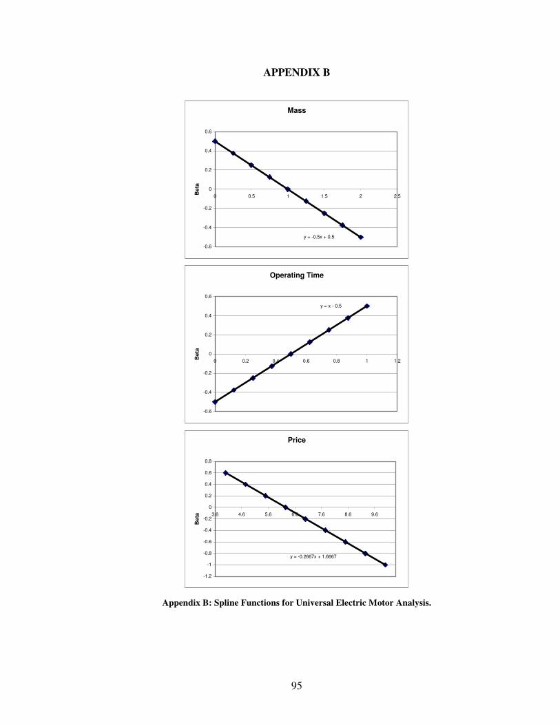
95

APPENDIX B

Mass

y = -0.5x + 0.5

-0.6

-0.4

-0.2

0

0.2

0.4

0.6

0 0.5 1 1.5 2 2.5Bet

a

Operating Time

y = x - 0.5

-0.6

-0.4

-0.2

0

0.2

0.4

0.6

0 0.2 0.4 0.6 0.8 1 1.2Bet

a

Price

y = -0.2667x + 1.6667

-1.2

-1

-0.8

-0.6

-0.4

-0.2

0

0.2

0.4

0.6

0.8

3.6 4.6 5.6 6.6 7.6 8.6 9.6

Bet

a

Appendix B: Spline Functions for Universal Electric Motor Analysis.

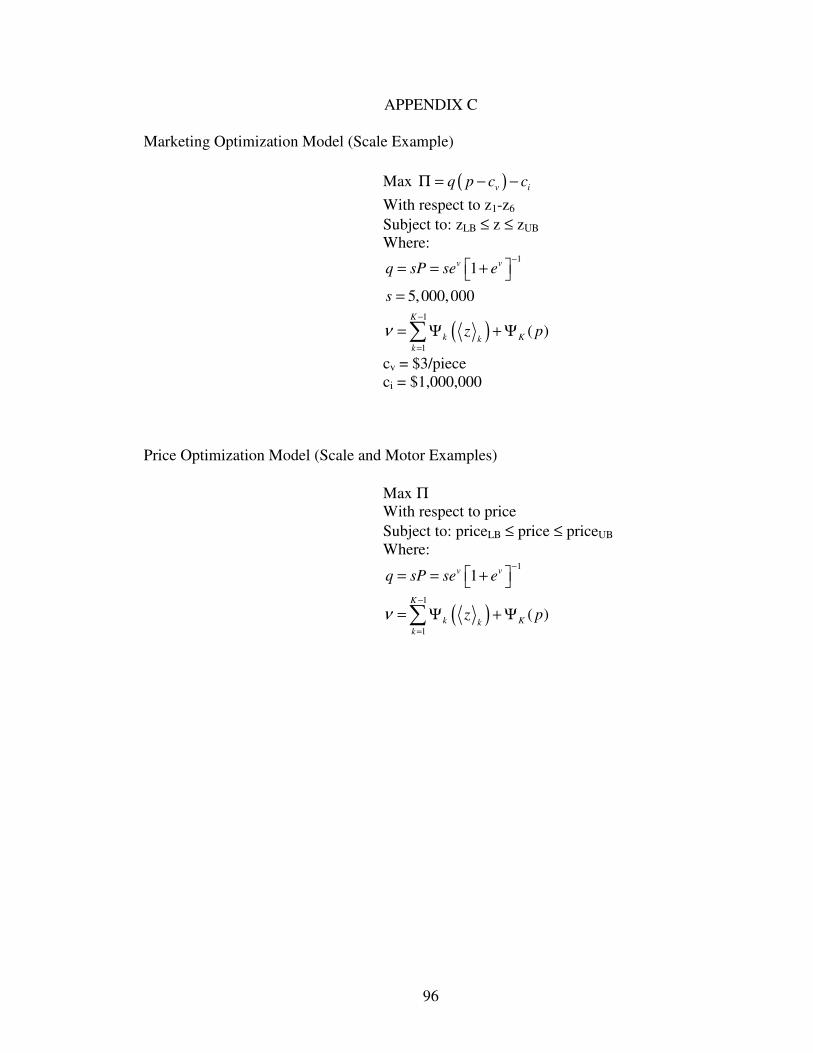
96

APPENDIX C

Marketing Optimization Model (Scale Example)

Max ( )v iq p c cΠ = − −

With respect to z1-z6

Subject to: zLB ≤ z ≤ zUB

Where:

( )

1

1

1

1

5,000,000

( )

v v

K

k Kkk

q sP se e

s

z pν

−

−

=

⎡ ⎤= = +⎣ ⎦=

= Ψ + Ψ∑ cv = $3/piece ci = $1,000,000

Price Optimization Model (Scale and Motor Examples)

Max Π With respect to price Subject to: priceLB ≤ price ≤ priceUB

Where:

( )

1

1

1

1

( )

v v

K

k Kkk

q sP se e

z pν

−

−

=

⎡ ⎤= = +⎣ ⎦

= Ψ + Ψ∑

97

REFERENCES

[1] Braun, R.D., Moore, A.A., and Kroo, I.M., 1996. “Use of Collaborative Optimization

Architecture for Launch Vehicle Design,” Proceedings of the 6th

AIAA/NASA/USAF/ISSMO Symposium on Multidisciplinary Analysis and Optimization,

Bellevue, WA, pp. 306-318.

[2] Badhrinath, K., Madelone, J., Nagendra, S., Plybon, R.C., and Woodruff, M.,

“Preliminary System Design Optimization of Aircraft Engine.”

http://www.engineous.com/aerospace_cases.htm.

[3] Palloni, F., “A New Tool for Multidisciplinary CAE Simulations,”

http://www.nenastran.com/newnoran/confererncePaper.php.

[4] Cramer, E.J., Frank, P.D., Shubin, G.R., Dennis, J.E., JR, and Lewis, R.M., 1992. “On

Alternative Problem Formulations for Multidisciplinary Design Optimization,” AIAA-

92-4752, 4th Symposium on Multidisciplinary Analysis and Optimization, September 21-

23, Cleveland, Ohio.

[5] Cramer, E.J., Dennis, J.E.jr., Frank, P.D., Lewis, R.M., and Shubin, G.R., 1994.

“Problem Formulation for Multidisciplinary Optimization,” SIAM Journal on

Optimization, 4(4), pp. 754-776.

[6] Kumar, D., Kim, H.M., and Chen, W., 2006. “Multi-level Optimization for Enterprise

Driven Decision-based Product Design,” to appear in Decision Making in Engineering

Design, W. Chen, K. Lewis, and L.C. Schmidt, editors, ASME Press, New York.

[7] Braun, R.D., Gage, P., Kroo, I., and Sobieski, I., 1996. “Implementation and

Performance Issues in Collaborative Optimization,” AIAA-96-4017, Proceedings of the

6th AIAA/NASA/USAF/ISSMO Symposium on Multidisciplinary Analysis and

Optimization, Bellevue, WA, pp.295-305.

[8] Kroo, I., Altus, S., Braun, R.D., Gage, P., and Sobieski, I., 1994. “Multidisciplinary

Optimization Methods for Aircraft Preliminary Design,” AIAA-94-4325-CP,

Proceedings of the 5th AIAA/NASA/USAF/ISSMO Symposium on Multidisciplinary

Analysis and Optimization, Panama City, FL, pp. 697-707.

98

[9] Balling, R.J. and Sobieszczanski-Sobieski, J., 1994. “Optimization of Coupled

Systems: A Critical Overview of Approaches,” AIAA-94-4330-CP, Proceedings of the

5th AIAA/NASA/USAF/ISSMO Symposium on Multidisciplinary Analysis and

Optimization, Panama City, FL, pp. 753-773.

[10] Sobieski, I. and Kroo, I., 1996. “Aircraft Design Using Collaborative Optimization,”

AIAA-96-0715, AIAA Meeting Papers, Reno, NV.

[11] Gu, X., Renaud, J., Ashe, L., Batill, S., Budhiraja, A., and Krajewski, L., 2002.

“Decision-based Collaborative Optimization,” Transactions of ASME: Journal of

Mechanical Design, 124(3), pp. 1-13.

[12] Graham, R.L., Lawler, E.L., Lenstra, J.K., Rinnooy Kan, A.H.G., 1979.

“Optimization and Approximation in Deterministic Sequencing and Scheduling: A

Survey,” Annals of Discrete Mathematics, 5, pp. 287-326.

[13] Leung, J.Y.-T., 2004. Handbook of Scheduling: Algorithms, Models, and

Performance Analysis, Chapman & Hall, CRC Press LLC, Boca Raton, FL, pp. 6-9.

[14] Kim, H.M., Rideout, D.G., Papalambros, P.Y., and Stein, J.L., 2003. “Analytical

Target Cascading in Automotive Vehicle Design,” Transactions of ASME: Journal of

Mechanical Design, 125(3), pp. 481-489.

[15] Kim, H.M., Michelena, N.F., and Jiang, T., 2000. “Target Cascading in Optimal

System Design,” DETC2000/DAC-14265, Proceedings of DETC ASME Design

Engineering Technical Conference, Baltimore, MD.

[16] Michalek, J.J., Feinberg, F.M., and Papalambros, P.Y., 2005. “Linking Marketing

and Engineering Product Design Decisions via Analytical Target Cascading,” Journal of

Product Innovation Management, 22, pp. 42-62.

[17] Michalek, J.J., Ceryan, O., Papalambros, P.Y., and Koren, Y., 2006. “Balancing

Marketing and Manufacturing Objectives in Product Line Design,” to appear in the

ASME Journal of Mechanical Design.

[18] Hazelrigg, G.A., 1996. Systems Engineering: An Approach to Information-Based

Design, Prentice Hall, Upper Saddle River, NJ.

[19] Li, H. and Azarm, S., 2000. “Product Design Selection Under Uncertainty and with

Competitive Advantage,” Journal of Mechanical Design, 122 (4), pp. 411-418.

99

[20] Li, H. and Azarm, S., 2002. “An Approach for Product Line Design Selection Under

Uncertainty and Competition,” Transactions of ASME: Journal of Mechanical Design,

124, pp.385-392.

[21] Maddulapalli, K., Azarm, S., and Boyars, A., 2002. “Interactive Product Design

Selection with an Implicit Value Function,” DETC02/DAC-34080, Proceedings of DETC

ASME Design Engineering Technical Conference, Montreal, Canada.

[22] Gupta, S.K. and Samuel, A.K., 2001. “Integrating Market Research with the Product

Development Process: A Step Towards Design for Profit,” DETC01/DFM-21202,

Proceedings of DETC ASME Design Engineering Technical Conference, Pittsburgh, PA.

[23] Pan, J. and Diaz, A.R., 1990. “Some Results in Optimization of Nonhierarchic

Systems,” Transactions of ASME: Journal of Mechanical Design, 112, pp. 399-405.

[24] Simpson, T.W., 2003. “Product Platform Design and Optimization: Status and

Promise,” DETC03/DAC-48717, Proceedings of DETC ASME Design Engineering

Technical Conference, Chicago, IL.

[25] Messac, A. and Chen, W., 2000. “The Engineering Design Discipline. Is its

Confounding Lexicon Hindering its Evolution?” Journal of Engineering Evaluation and

Cost Analsyis, Decision-based Design: Status and Promise, 3, pp. 67-83.

[26] Nagle, T. and Holden, R.K., 2002. The Strategy and Tactics of Pricing, 3rd edition,

Prentice Hall, Upper Saddle River, New Jersey.

[27] Smith, P.G. and Reinertsen, D.G., 1991. Developing Products in Half the Time, Van

Nostrand Reinhold, New York, NY, pp. 17-42.

[28] Otto, K. and Wood, K., 2001. Product Design: Techniques in Reverse Engineering

and New Product Development, Prentice Hall, Upper Saddle River, NJ, pp. 803-805,

Chap. 16.

[29] McAllister, C. and Simpson, T., 2003. “Multidisciplinary Robust Design

Optimization of an Internal Combustion Engine,” Transactions of ASME: Journal of

Mechanical Design, 125, pp.124-130.

[30] Wassenaar, H.J. and Chen, W., 2001. “An Approach to Decision-Based Design,”

DETC01/DTM-21683, Proceedings of DETC ASME Design Engineering Technical

Conference, Pittsburgh, PA.

100

[31] Sues, R.H., Shin, Y., and Wu, Y.T., 2005. “Applications of Reliability-Based Design

Optimization,” Engineering Design Reliability Handbook, CRC Press, Boca Raton,

Florida.

[32] Azarm, S. and Narayanan, S., 2000. “A Multi-objective Interactive Sequential

Hybrid Optimization Technique for Design Decision Making,” Engineering

Optimization, 32, pp. 485-500.

[33] Tappeta, R. and Renaud, J., 1997. “Multi-objective Collaborative Optimization,”

Transactions of ASME: Journal of Mechanical Design, 119(3), pp. 403-41.

[34] Clarkson, J. and Eckert, C., (eds.) 2005. “Design Process Improvement: A review of

current practice,” Springer-Verlag London Limited, London, England.

[35] Daganzo, C., 1979. “Multinomial Probit: The Theory and Its Applications to

Demand Forecasting,” Academic Press Inc., New York.

[36] Hensher, D.A. and Johnson, L.W., 1981. “Applied Discrete-Choice Modeling,”

Halsted Press, New York.

[37] Simpson, T.W., Maier, J. and Mistree, F., 1999. “A Product Platform Concept

Exploration Method for Product Family Design,” DETC99/DTM-8761, Proceedings of

DETC ASME Design Engineering Technical Conference, Las Vegas, Nevada.

[38] Simpson, T.W., 1998. “A Concept Exploration Method for Product Family Design,”

PhD Dissertation, Georgia Institute of Technology.

[39] Cooper, A.B., Georgiopoulos, P., Kim, H.M. and Papalambros, P.Y., 2003.

“Analytical Target Setting: An Enterprise Context in Optimal Product Design,”

DETC2003/DAC-48734, Proceedings of DETC ASME Design Engineering Technical

Conference, Chicago, Illinois.

Documents

Classifying and Comparing Design Optimization Problems