Classifier Evaluation

Vasileios Hatzivassiloglou

University of Texas at Dallas

Hash tables

• A hash table or associative array implements efficiently a function with a very large domain but relatively few recorded values

• Example: Map names to phone numbers– Although there are many possible names,

only a few will be stored in a particular phone book

Implementing hash tables• A hash table works by using a hash function to

translate the input (keys) to a small range of buckets– For example, h(n) = n mod k where k is the size of

hash table

• Collisions can occur when different keys are mapped to the same bucket, and must be resolved

• Many programming languages directly support hash tables

Example hash table

FASTA after step 1

FASTA – Step 2

• Group together hot spots on the same diagonal. This creates a partial alignment with matches and mismatches (no indels).

• Keep the 10 best diagonal runs

• If a hot spot matches at position i in S and position j in T, it will be on the (i-j)th diagonal

• Sort hot spots by i-j to group them

FASTA – Step 3

• Rescore exact matches using realistic substitution penalties (from a set such as PAM250 for proteins)

• Trim and extend hot spots according to substitution penalties, allowing “good” mismatches

The PAM matrices

• From observing closely related proteins in evolution, we can estimate the likelihood than one amino acid mutates to another

• Normalize these probabilities by PAM (Percentage of Acceptable Mutations in 100 amino-acids)

• The PAM0 matrix is the identity matrix• The PAM1 matrix diverges slightly from the

identity matrix

Calculating PAM matrices• If we have PAM1, then

– PAMN = (PAM1)N

– A Markov chain of independent mutations

• The PAM250 matrix has been found empirically most useful

• At this evolutionary distance, 80% of amino acids are changed

• Change varies according to class (from only 45% to 94%)

• Some amino acids are no longer good matches with themselves

FASTA after Steps 2 and 3

FASTA – Step 4

• Starting from the best diagonal run, look at nearby diagonal runs and incorporate non-overlapping hot spots

• This extends the partial alignment with some insertions and deletions

• We only look a limited distance from the best diagonal run

FASTA after Step 4

FASTA – Step 5

• Run the full dynamic programming alignment algorithm in a band around the extended best diagonal run

• Only consider matches within w positions on either side of the extended best diagonal run

• Typically, w is 16, and 32n ≪ n2

FASTA final step

BLAST• Basic Local Alignment Search Tool• Uses words like FASTA, but allows for approximate

matches of words to create high scoring pairs (HSPs)

• Usually longer words (k=3 for proteins, 11 for DNA)• HSPs are combined on the same diagonal and

extended• Reports local alignments based on one HSP or a

combination of two close HSPs• Variations allow gaps and pattern search

Alignment as classification

• Alignment can be viewed as– A function that produces similarity values

between any two strings• These similarity values can then be used to inform

classifiers and clustering programs

– A binary classifier: Any two strings are classified as related/similar or not

• Requires the use of a threshold• The threshold can be fixed or depend on the

context and application

Measuring performance

• Done on a test set separate from the training set (the examples with known labels)

• We need to know (but not make available to the classifier) the class labels in the test set, in order to evaluate the classifier’s performance

• Both sets must be representative of the problem instances – not always the case

Contingency tables

• Given a n-way classifier, a set with labels assigned by the classifier and correct, known labels we construct a n×n contingency table counting all combinations of true/assigned classes

2×2 Contingency Table

• Binary classification in this example

True class

Classifier-assigned class

Spam Not spam

Spam a c

Not spam b d

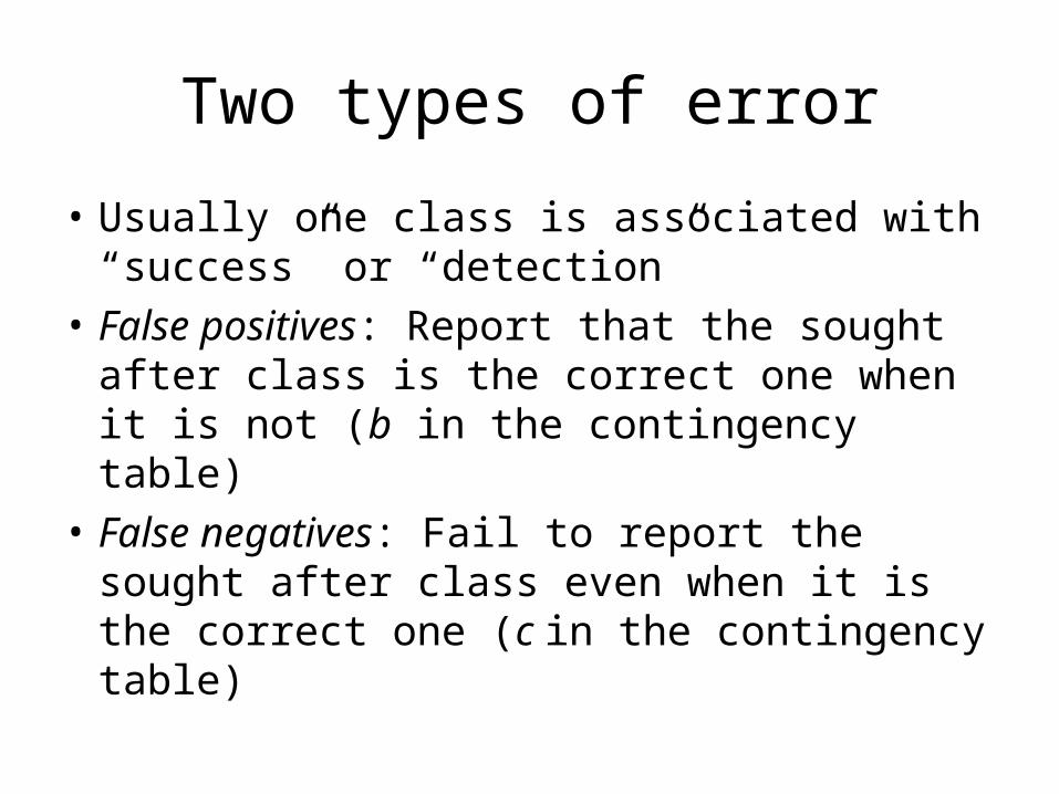
Two types of error

• Usually one class is associated with “success” or “detection”

• False positives: Report that the sought after class is the correct one when it is not (b in the contingency table)

• False negatives: Fail to report the sought after class even when it is the correct one (c in the contingency table)

Performance measures

• Accuracy: How often is the classification correct?

• A = (a+d)/N, where N is the size of the scored set (N=a+b+c+d)

• Problem: If the a priori probability of one class is much higher, we are usually better off just predicting that class, which is not a very meaningful classifier

• E.g., in a disease detection test

Accounting for rare classes

• Assign a cost to each error and measure the expected error– Normalize for fixed N to make results

comparable across experiments

• Measure separate error rates– Precision P=a/(a+b)– Recall (or sensitivity) R=a/(a+c)– Specificity d/(d+b)

FNFP CN

cC

N

b