Embed Size (px)
Citation preview

Classification of stop consonant place of articulation
by
Atiwong Suchato
B.Eng., Chulalongkorn University (1998)
S.M., Massachusetts Institute of Technology (2000)
Submitted to the Department of Electrical Engineering and Computer Science
in partial fulfillment of the requirements for the degree of M
Doctor of Philosophy
at the
Massachusetts Institute of Technology
June 2004
@ Massachusetts Institute of Technology 2004. All rights reserved.
Author
Certified by
Accepted by
ASSACHUSETTS INSTITUTEOF TECHNOLOGY
JUL 2 6 2004
LIBRARIES
/Department of Electric ngineering and Computer Science
April 27t', 2004
Kenneth N. Stevens
ClarenweJ. LeBel Professor of Electrical Engineeringan4 Professor of Healtl-,Sciences & Technology
Thepigj$upervisor
Arthur C. Smith
Chairman, Departmental Committee on Graduate Students
BARKER

This page is intentionally left blank.
2

Classification of Stop Consonant Place of Articulation
byAtiwong Suchato
Submitted to the Department of Electrical Engineering and Computer Scienceon April 27 th, 2004, in partial fulfillment of the
requirements for the degree ofDoctor of Philosophy in Electrical Engineering and Computer Science
Abstract
One of the approaches to automatic speech recognition is a distinctive feature-basedspeech recognition system, in which each of the underlying word segments is representedwith a set of distinctive features. This thesis presents a study concerning acousticattributes used for identifying the place of articulation features for stop consonantsegments. The acoustic attributes are selected so that they capture the informationrelevant to place identification, including amplitude and energy of release bursts, formantmovements of adjacent vowels, spectra of noises after the releases, and some temporalcues.
An experimental procedure for examining the relative importance of theseacoustic attributes for identifying stop place is developed. The ability of each attribute toseparate the three places is evaluated by the classification error based on the distributionsof its values for the three places, and another quantifier based on F-ratio. These twoquantifiers generally agree and show how well each individual attribute separates thethree places.
Combinations of non-redundant attributes are used for the place classificationsbased on Mahalanobis distance. When stops contain release bursts, the classificationaccuracies are better than 90%. It was also shown that voicing and vowel frontnesscontexts lead to a better classification accuracy of stops in some contexts. When stops arelocated between two vowels, information on the formant structures in the vowels on bothsides can be combined. Such combination yielded the best classification accuracy of95.5%. By using appropriate methods for stops in different contexts, an overallclassification accuracy of 92.1% is achieved.
Linear discriminant function analysis is used to address the relative importance ofthese attributes when combinations are used. Their discriminating abilities and theranking of their relative importance to the classifications in different vowel and voicingcontexts are reported. The overall findings are that attributes relating to the burstspectrum in relation to the vowel contribute most effectively, while attributes relating toformant transition are somewhat less effective. The approach used in this study can beapplied to different classes of sounds, as well as stops in different noise environments.
Thesis supervisor: Professor Kenneth Noble StevensTitle: Clarence J. LeBel Professor of Electrical Engineering and Professor of HealthSciences and Technology
3

This page is intentionally left blank.
4

Acknowledgement
It takes more than determination and hard work for the completion of this thesis.
Supports I received from many people through out my years here at MIT undeniably
played an important role. My deepest gratitude clearly goes to Ken Stevens, my thesis
supervisor and my teacher. His genuine interest in the field keeps me motivated, while his
kindness and understanding always help me go through hard times. Along with Ken, I
would like to thank Jim Glass and Michael Kenstowicz for the time they spent on reading
several drafts of this thesis and their valuable comments. I would like to specially thank
Janet Slifka for sharing her technical knowledge, as well as her study and working
experience, and Arlene Wint for her help with many administrative matters. I could
hardly name anything I have accomplished during my doctoral program without their
help. I also would like to thank all of the staffs in the Speech Communication Group,
including Stefanie Shattuck-Hufnagel, Sharon Manuel, Melanie Matthies, Mark Tiede,
and Seth Hall, as well as all of the students in the group, especially Neira Hajro, Xuemin
Chi, and Xiaomin Mou.
My student life at MIT would have been much more difficult without so many
good friends around me. Although it is not possible to name all of them in this space, I
would like to extend my gratitude to them all and wish them all the best.
I would like to thank my parents who are always supportive. Realizing how much
they want me to be successful is a major drive for me. Also, I would like to thank Mai for
never letting me give up, and for always standing by me.
Finally, I would like to thank Anandha Mahidol Foundation for giving me the
opportunity to pursue the doctoral degree here at MIT.
This work has been supported in part by NIH grant number DC 02978
5

This page is intentionally left blank.
6

Table of Contents
Chapter 1 Introduction............................................................................................ 17
1.1 M otivation ..................................................................................................... 171.2 Distinctive feature-based Speech Recognition System.................................. 191.3 An Approach to Distinctive Feature-based speech recognition.................... 201.4 Literature Review.......................................................................................... 251.5 Thesis Goals.................................................................................................. 291.6 Thesis Outline ................................................................................................ 29
Chapter 2 Acoustic Properties of Stop Consonants............................................... 31
2.1 The Production of Stop Consonants ............................................................. 312.2 Unaspirated Labial Stop Consonants ........................................................... 332.3 Unaspirated Alveolar Stop Consonants ......................................................... 342.4 Unaspirated Velar Stop Consonants ............................................................. 342.5 Aspirated Stop Consonants ........................................................................... 362.6 Chapter Summary .......................................................................................... 36
Chapter 3 Acoustic Attribute Analysis.................................................................. 37
3.1 SP D atabase .................................................................................................. 383.2 Acoustic Attribute Extraction ...................................................................... 40
3.2.1 Averaged Power Spectrum ........................................................................ 403.2.2 Voicing Onsets and Offsets ...................................................................... 413.2.3 Measurement of Formant Tracks ............................................................. 41
3.3 Acoustic Attribute Description ...................................................................... 433.3.1 Attributes Describing Spectral Shape of the Release Burst...................... 433.3.2 Attributes Describing the Formant Frequencies ........................................ 483.3.3 Attributes Describing the spectral shape between the release burst and thevoicing onset of the following vowel.................................................................... 503.3.4 Attributes Describing Some Temporal Cues ............................................ 50
3.4 Statistical Analysis of Individual Attributes ................................................. 523 .4 .1 R esu lts........................................................................................................... 5 73.4.2 Comparison of Each Acoustic Attribute's Discriminating Property ...... 933.4.3 Correlation Analysis ................................................................................. 96
3.5 Chapter Summary .......................................................................................... 98
Chapter 4 Classification Experiments ..................................................................... 101
4.1 Classification Experiment Framework ........................................................... 1024.1.1 Acoustic Attribute Selection....................................................................... 1024.1.2 Classification Result Evaluation................................................................. 1044.1.3 Statistical Classifier .................................................................................... 1054.1.4 Classification Context................................................................................. 106
4.2 LOOCV Classification Results for Stops Containing Release Burst.............. 107
7
4.3 LOOCV Classification Using Only Formant Information ............................. 1104.4 Effect of Context Information......................................................................... 1124.5 Classification of Stops that have Vowels on Both Sides ................................ 115
4.5.1 Attribute-level Combination ....................................................................... 1164.5.2 Classifier-level Combination ...................................................................... 121
4.6 Evaluation on the SP Database ....................................................................... 1304.7 Chapter Summary ........................................................................................... 139
Chapter 5 Discriminant Analysis............................................................................. 141
5.1 LDA Overview................................................................................................ 1415.2 Contribution Analysis on CV tokens in the ALL dataset ............................... 1445.3 Contribution Analysis on VC tokens in the ALL dataset ............................... 1485.4 Contribution Analysis on CV tokens with known voicing contexts............... 1525.5 Contribution Analysis on CV tokens with known vowel frontness contexts. 1545.6 Contribution Analysis on VC tokens with known voicing contexts............... 1545.7 Contribution Analysis on VC tokens with known vowel frontness contexts. 1555.8 Summary on the Contribution to the Place Classification of the AcousticAttributes in Different Contexts ................................................................................. 1565.9 Chapter Summary ........................................................................................... 157
Chapter 6 Conclusion .............................................................................................. 159
6.1 Summary and Discussion................................................................................ 1596.2 Contributions................................................................................................... 1696.3 Future W ork .................................................................................................... 171
B ib lo g rap h y ................................................................................................................. 17 5
Appendix A Sentences in the SP database .................................................................. 180
8

List of Figures
Figure 1-1: Distinctive feature-based approach for representing words from analogacou stic sign al...........................................................................................................2 1
Figure 1-2: Illustration of an approach to distinctive feature-based speech recognitionsy stem ....................................................................................................................... 2 1
Figure 1-3: A diagram for a distinctive feature-based speech recognition system with thefeedback path. (After Stevens, 2002).................................................................... 24
Figure 2-1: A spectrogram of the utterance lax g ae gi. The movement of the articulatorsthat is reflected in the acoustic signal in the area marked (1), (2) and (3) is explainedin th e text ab ove........................................................................................................ 33
Figure 2-2: Spectrogram of the utterance of (a) lb aa b/, (b) lb iy bi, (c) Id aa dl, (d) Id iydl, (e) Ig aa gi, and (f) Ig iy g/. (The horizontal axes in all plots show time in second).......................................................................................................... . . . . . ............ 35
Figure 3-1: Examples of average power spectra of stops with the three places ofarticulation. The values of Ahi, A23, and Amax23 (calculated from these samplespectra) are shown by the location in the direction of the dB axis of their associatedhorizontal lines.......................................................................................................... 47
Figure 3-2: An example of CLSDUR and VOT of the consonant /k/ in a portion of awaveform transcribed as /1 uh k ae t/. CLSDUR is the time interval between thevoicing offset of the vowel /uh/ to the release of the /k/ burst. VOT is the timeinterval between the release of the /k/ burst to the voicing onset of the vowel /ae/. 51
Figure 3-3: A diagram showing an example of a box-and-whiskers plot used in this study................................................................................................................................... 5 3
Figure 3-4 : Box-and-whiskers plot and statistics of Av-Ahi values for the three places ofarticu latio n ................................................................................................................ 5 8
Figure 3-5 : Box-and-whiskers plot and statistics of Ahi-A23 values for the three placesof articu lation ............................................................................................................ 59
Figure 3-6 : Box-and-whiskers plot and statistics of Av-Amax23 values for the threeplaces of articulation .............................................................................................. 60
Figure 3-7 : Box-and-whiskers plot and statistics of Avhi-Ahi values for the three placesof articu lation ............................................................................................................ 6 1
Figure 3-8 : Box-and-whiskers plot and statistics of Av3-A3 values for the three places ofarticulation ................................................................................................................ 62
Figure 3-9 : Box-and-whiskers plot and statistics of Av2-A2 values for the three places ofarticu latio n ................................................................................................................ 64
Figure 3-10 : Box-and-whiskers plot and statistics of Ehi-E23 values for the three placesof articulation ............................................................................................................ 65
Figure 3-11 : Box-and-whiskers plot and statistics of VOT values for the three places ofarticu lation ................................................................................................................ 6 6
Figure 3-12 : Box-and-whiskers plot and statistics of VOT values for 'b', 'd' and 'g' ... 68Figure 3-13 : Box-and-whiskers plot and statistics of VOT values for 'p', 't' and 'k' .... 68Figure 3-14 : Box-and-whiskers plot and statistics of clsdur values for the three places
o f articulation ............................................................................................................ 70
9

Figure 3-15 : Box-and-whiskers plot and statistics of Flo values for the three places ofarticu latio n ................................................................................................................ 7 1
Figure 3-16 : Box-and-whiskers plot and statistics of F2o values for the three places ofarticu latio n ................................................................................................................ 7 2
Figure 3-17 : Box-and-whiskers plot and statistics of F2o values where the vowels arefront vowels for the three places of articulation .................................................. 74
Figure 3-18 : Box-and-whiskers plot and statistics of F2o values where the vowels areback vowels for the three places of articulation................................................... 74
Figure 3-19 : Box-and-whiskers plot and statistics of F2b values for the three places ofarticu lation ................................................................................................................ 7 5
Figure 3-20 : Box-and-whiskers plot and statistics of F3o values for the three places ofarticu latio n ................................................................................................................ 7 7
Figure 3-21 : Box-and-whiskers plot and statistics of F3b values for the three places ofarticu lation ................................................................................................................ 7 8
Figure 3-22 : Box-and-whiskers plot and statistics of dF2 values for the three places ofarticu lation ................................................................................................................ 80
Figure 3-23 : Box-and-whiskers plot and statistics of dF2 values where the vowels arefront vowels for the three places of articulation .................................................. 81
Figure 3-24 : Box-and-whiskers plot and statistics of dF2 values where the vowels areback vowels for the three places of articulation..................................................... 81
Figure 3-25 : Box-and-whiskers plot and statistics of dF2b values for the three places ofarticu lation ................................................................................................................ 8 3
Figure 3-26 : Box-and-whiskers plot and statistics of dF3 values for the three places ofarticu lation ................................................................................................................ 84
Figure 3-27: Box-and-whiskers plot and statistics of dF3b values for the three places ofarticu latio n ................................................................................................................ 85
Figure 3-28 : Box-and-whiskers plot and statistics of F3o-F2o values for the three placeso f articu lation ............................................................................................................ 8 7
Figure 3-29 : Box-and-whiskers plot and statistics of F3b-F2b values for the three placesof articu lation ............................................................................................................ 8 8
Figure 3-30: Box-and-whiskers plot and statistics of cgFlOa values for the three places ofarticu lation ................................................................................................................ 9 0
Figure 3-31: Box-and-whiskers plot and statistics of cgF20a values for the three places ofarticu lation ................................................................................................................ 9 1
Figure 3-32: Box-and-whiskers plot and statistics of cgFa values for the three places ofarticu lation ................................................................................................................ 9 2
Figure 3-33: Comparison between the F-ratios and the ML classification errorprobabilities, P(err), of all of the acoustic attributes. Note that, the ML classificationerror probabilities are plotted in the form of l-P(err). Both are scaled so that themaximal values are at 100%, while the minimal values are at 0%....................... 96
Figure 4-1: Valid acoustic attribute subsets. Valid subsets are constructed fromcombining four smaller subsets, one from each group (column). {Common subset)is always used as the subset from the first column. Either {Av3-A3} or {Av2-A2}must be picked from the second column due to their high correlation. The subsetslisted in the third column are all of the possible combinations among cgFa, cgFlOa,and cgF20a. In the last column, the listed subsets are all of the possible
10

combinations among F2o, F2b, F3o, F3b, F3o-F2o, and F3b-F2b in which none ofthe acoustic attributes are linear combinations of any other acoustic attributes in thesame subset and the information about a formant frequency at a certain time point isu sed o n ce ................................................................................................................. 10 3
Figure 4-2: Classification accuracy percentage of the place of articulation of stopconsonants with release bursts using the combined classifiers under the product ruleand the sum rule, when the weight used for the posterior probability obtained fromthe V C classifier varies from 0 to 1 ........................................................................ 124
Figure 4-3: Classification accuracy percentage of the place of articulation of stopconsonants using the combined classifiers under the product rule and the sum rule,when the weight used for the posterior probability obtained from the VC classifiervaries from 0 to 1. The information about release bursts is not used. .................... 127
Figure 4-4: Place of articulation classification process for the qualified tokens in the SPd atab ase ................................................................................................................... 13 1
Figure 4-5: Distribution of the classification error ......................................................... 136Figure 4-6: Histogram of the posterior probabilities corresponding to the hypothesized
place of articulation. The top histogram shows the number of the correctly classifiedstop consonants in different probability ranges. The bottom histogram shows thenumber of the incorrectly classified stop consonants in different probability ranges.................................................................................................................................. 1 3 8
Figure 4-7: Percentage of the correctly classified stop consonants in different probabilityran g e s ...................................................................................................................... 13 8
Figure 5-1: Scatter plot of the two canonical variables for CV tokens from the ALLd ataset ..................................................................................................................... 14 6
Figure 5-2: Scatter plot of the two canonical variables for VC tokens from the ALLd ataset ..................................................................................................................... 15 0
Figure 6-1: Relationship between the classification accuracy of stops in the entire SPdatabase and the classification accuracy of the excluded stops .............................. 168
Figure 6-2: Spectrograms of an utterance transcribed as 'Go get it at the bookstore-' withno added noise (Top), and with 28dB Signal-to-Noise Ratio white noise (Bottom).................................................................................................................................. 17 3
Figure 6-3: A scatter plot comparing the ML classification error probabilities based onAv-Ahi and Av-Amax23 for clean speech and for speech in different levels of whiten o ise ........................................................................................................................ 17 4
11

List of Tables
Table I -1: Feature values for the stop consonants in English ..................................... 20Table 3-1: Distribution of stop consonants in the SP database...................................... 40Table 3-2 Comparison of the means of Av-Ahi between the front and back vowel cases
.......................................... .................................... . 58Table 3-3 Comparison of the means of Ahi-A23 between the front and back vowel cases
................................................. 59Table 3-4 : Comparison of the means of Av-Amax23 between the front and back vowel
c ase s .......................................................................................................................... 6 0Table 3-5 : Comparison of the means of Avhi-Ahi between the front and back vowel
c ase s .......................................................................................................................... 6 1Table 3-6 Comparison of the means of Av3-A3 between the front and back vowel cases
. .................................................... .............. 63Table 3-7 : Comparison of the means of Av2-A2 between the front and back vowel cases
. ...................................... ........................................................... . 64Table 3-8 : Comparison of the means of Ehi-E23 between the front and back vowel cases
................................................ 65Table 3-9: Comparison of the means of VOT between the front and back vowel cases. 66Table 3-10 : Comparison of the means of clsdur between the front and back vowel cases
Tab ....e 3 :C m a.s..t.m.sfF.bt e nt ef .t n ba k. w . . 70Table 3-12 : Comparison of the means of Flo between the front and back vowel cases. 71Table 3-12 : Comparison of the means of F2o between the front and back vowel cases. 73Table 3-13 Comparison of the means of F2b between the front and back vowel cases. 75Table 3-14: Comparison of the means of F3o between the front and back vowel cases. 77Table 3-15 : Comparison of the means of F3b between the front and back vowel cases. 78Table 3-16: Comparison of the means of dF2 between the front and back vowel cases. 80Table 3-17 : Comparison of the means of dF2b between the front and back vowel cases 83Table 3-18 : Comparison of the means of dF3 between the front and back vowel cases. 84Table 3-19 : Comparison of the means of dF3b between the front and back vowel cases 85Table 3-20 :Comparison of the means of F3o-F2o between the front and back vowel
c ase s .......................................................................................................................... 8 7Table 3-21 : Comparison of the means of F3b-F2b between the front and back vowel
c ase s .......................................................................................................................... 8 8Table 3-22: Comparison of the means of cgFlOa between the front and back vowel cases
. ...... .............. .................................. 90Table 3-23: Comparison of the means of cgF20a between the front and back vowel cases
.......................................................... ............................................... .91Table 3-24: Comparison of the means of cgFa between the front and back vowel cases 92Table 3-25: normalized F-ratios of every acoustic attribute, sorted in descending order. 95Table 3-26: Maximum likelihood classification error of every acoustic attribute, sorted in
ascend in g order ......................................................................................................... 95Table 3-27: Highly correlated attribute pairs (p2 > 0.80) across different CV contexts ... 97Table 3-28: Highly correlated attribute pairs (p 2> 0.80) across different VC contexts ... 97
12

Table 4-1: Attribute subsets yielding the best CV token classification results in theircorresponding vowel and voicing contexts. Common attribute subset consists of Av-Ahi, Ahi-A23, Av-Amax23, Avhi-Ahi, Ehi-E23, vot, Flo, dF2, dF3, dF2b, dF3b 108
Table 4-2: Confusion matrices of the best CV token classification in different vowel andvoicing contexts. The attribute subset used in each context is shown in the abovetab le ......................................................................................................................... 10 8
Table 4-3: Attribute subsets yielding the best VC token classification results in theircorresponding vowel and voicing contexts. Common attribute subset consists of Av-Ahi, Ahi-A23, Av-Amax23, Avhi-Ahi, Ehi-E23, cls_dur, Flo, dF2, dF3, dF2b, dF3b................................................................................................................................. 10 9
Table 4-4: Confusion matrices of the best VC token classification in different vowel andvoicing contexts. The attribute subset used in each context is shown in the abovetab le ......................................................................................................................... 10 9
Table 4-5: Confusion matrices of the best CV token classification in different vowel andvoicing contexts where the attributes used are obtained from the information onformants only. The attribute subset used is 'Flo', 'F2o', 'F3o', 'dF2', and 'dF3'. 111
Table 4-6: Confusion matrices of the best VC token classification in different vowel andvoicing contexts where the attributes used are obtained from the information onformants only. The attribute subset used is 'Flo', 'F2o', 'F3o', 'dF2', and 'dF3'. 111
Table 4-7: Classification accuracies in the context-specific training case and the context-free training case for CV tokens across all voicing and frontness contexts............ 113
Table 4-8: Comparison between the classification accuracies of CV tokens when somecontexts are known and when they are not known. ................................................ 113
Table 4-9: Classification accuracies in the context-specific training case and the context-free training case for VC tokens across all voicing and frontness contexts............ 114
Table 4-10: Comparison between the classification accuracies of VC tokens when somecontexts are known and when they are not known. ................................................ 115
Table 4-11: Confusion matrix of the place of articulation classification of CV tokenswhose stop consonants also have adjacent vowels on the left side. The informationabout the release bursts is used. .............................................................................. 118
Table 4-12: Confusion matrix of the place of articulation classification of VC tokenswhose stop consonants also have adjacent vowels on the right side. The informationabout the release bursts is used. .............................................................................. 118
Table 4-13: Confusion matrix of the place of articulation classification of CV tokenswhose stop consonants also have adjacent vowels on the left side. Only theinformation about the formant structure of the vowels is used............................... 118
Table 4-14: Confusion matrix of the place of articulation classification of VC tokenswhose stop consonants also have adjacent vowels on the right side. Only theinformation about the formant structure of the vowels is used............................... 119
Table 4-15: Confusion matrix from place of articulation classification of stops withrelease bursts that have vowels on both sides. The acoustic attributes on both sidesof the stops, as well as the burst information, are used together in a singleclassification ........................................................................................................... 120
Table 4-16: Confusion matrix from place of articulation classification of stops that havevowels on both sides, where the burst information is not used. The acousticattributes on both sides of the stops are used together in a single classification. ... 120
13
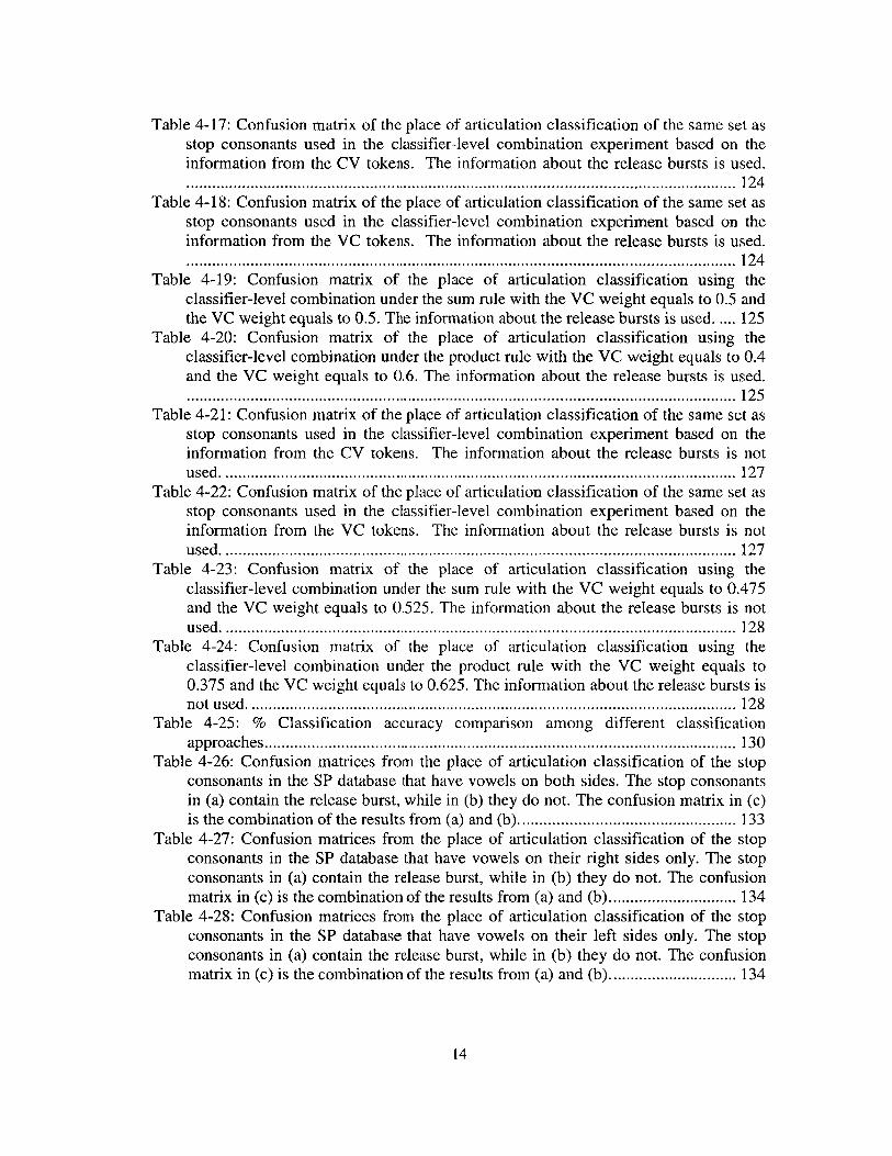
Table 4-17: Confusion matrix of the place of articulation classification of the same set asstop consonants used in the classifier-level combination experiment based on theinformation from the CV tokens. The information about the release bursts is used........................ ... .... ........ ..................................................... . 124
Table 4-18: Confusion matrix of the place of articulation classification of the same set asstop consonants used in the classifier-level combination experiment based on theinformation from the VC tokens. The information about the release bursts is used........................................ ................................ 124
Table 4-19: Confusion matrix of the place of articulation classification using theclassifier-level combination under the sum rule with the VC weight equals to 0.5 andthe VC weight equals to 0.5. The information about the release bursts is used. .... 125
Table 4-20: Confusion matrix of the place of articulation classification using theclassifier-level combination under the product rule with the VC weight equals to 0.4and the VC weight equals to 0.6. The information about the release bursts is used.
................................................125Table 4-21: Confusion matrix of the place of articulation classification of the same set as
stop consonants used in the classifier-level combination experiment based on theinformation from the CV tokens. The information about the release bursts is notu sed ......................................................................................................................... 12 7
Table 4-22: Confusion matrix of the place of articulation classification of the same set asstop consonants used in the classifier-level combination experiment based on theinformation from the VC tokens. The information about the release bursts is notu sed ......................................................................................................................... 12 7
Table 4-23: Confusion matrix of the place of articulation classification using theclassifier-level combination under the sum rule with the VC weight equals to 0.475and the VC weight equals to 0.525. The information about the release bursts is notu sed ......................................................................................................................... 12 8
Table 4-24: Confusion matrix of the place of articulation classification using theclassifier-level combination under the product rule with the VC weight equals to0.375 and the VC weight equals to 0.625. The information about the release bursts isn o t u sed ................................................................................................................... 12 8
Table 4-25: % Classification accuracy comparison among different classificationap p ro ach es............................................................................................................... 130
Table 4-26: Confusion matrices from the place of articulation classification of the stopconsonants in the SP database that have vowels on both sides. The stop consonantsin (a) contain the release burst, while in (b) they do not. The confusion matrix in (c)is the combination of the results from (a) and (b)................................................... 133
Table 4-27: Confusion matrices from the place of articulation classification of the stopconsonants in the SP database that have vowels on their right sides only. The stopconsonants in (a) contain the release burst, while in (b) they do not. The confusionmatrix in (c) is the combination of the results from (a) and (b).............................. 134
Table 4-28: Confusion matrices from the place of articulation classification of the stopconsonants in the SP database that have vowels on their left sides only. The stopconsonants in (a) contain the release burst, while in (b) they do not. The confusionmatrix in (c) is the combination of the results from (a) and (b).............................. 134
14

Table 4-29: Confusion matrices from the place of articulation classification of the stopconsonants in the SP database. The stop consonants in (a) contain the release burst,while in (b) they do not. The confusion matrix in (c) is the combination of the resultsfrom (a) and (b )....................................................................................................... 135
Table 5-1: Confusion matrix based on using the two canonical variables obtained fromLDA to classify the place of articulation of CV tokens from the ALL dataset ...... 147
Table 5-2: Standardized coefficients for the 1st and the 2nd discriminant functions withrespect the acoustic attributes used for classifying CV tokens in the ALL dataset 147
Table 5-3: Eigenvalues and dispersion percentages explained by the two discriminantfunctions for the CV tokens in the ALL dataset ..................................................... 147
Table 5-4: Contributions to the 1st, the 2 "d discriminant function, and the overalldiscrimination among the three places of articulation of the acoustic attributes usedfor the CV tokens in the A LL dataset ..................................................................... 148
Table 5-5: Confusion matrix based on using the two canonical variables obtained fromLDA to classify the place of articulation of VC tokens from the ALL dataset ...... 150
Table 5-6: Standardized coefficients for the 1st and the 2nd discriminant functions withrespect the acoustic attributes used for classifying VC tokens in the ALL dataset 151
Table 5-7: Eigenvalues and dispersion percentages explained by the two discriminantfunctions for the VC tokens in the ALL dataset ..................................................... 151
Table 5-8: Contributions to the 1st, the 2 discriminant function, and the overalldiscrimination among the three places of articulation of the acoustic attributes usedfor the V C tokens in the ALL dataset ..................................................................... 151
Table 5-9: The overall contribution to the total separation of the acoustic attributes usedfor CV tokens in (a) the V dataset and (b) the U dataset ........................................ 153
Table 5-10: The overall contribution to the total separation of the acoustic attributes usedfor CV tokens in (a) the F dataset and (b) the B dataset ......................................... 154
Table 5-11: The overall contribution to the total separation of the acoustic attributes usedfor VC tokens in (a) the V dataset and (b) the U dataset ........................................ 155
Table 5-12: The overall contribution to the total separation of the acoustic attributes usedfor VC tokens in (a) the F dataset and (b) the B dataset ......................................... 156
15

This page is intentionally left blank.
16

Chapter 1
Introduction
1.1 Motivation
The problem of automatic speech recognition has been approached by researchers in
various ways. One of the most prevalent methods is a statistical method in which speech
recognizers learn the patterns of the speech units expected in incoming utterances from
some sets of examples and then try to match the incoming speech units with the patterns
learned. Different choices of units of speech that are used to represent sounds in the
incoming utterance have been examined [Davis and Mermelstein, 1980] [Jankowski,
Hoang-Doan, and Lippman, 1995]. These representations include MFCCs, LPCs,
wavelets [Malbos, Baudry, and Montresor, 1994], and other spectral-based
representations [Kingsbury, Morgan, and Greenberg, 1998] [Hermansky, and Morgan,
1994]. This approach to automatic speech recognition does not use much knowledge of
human speech production, and the performance of the recognizer relies heavily on the
training examples. The recognition performance is robust when the recognizer tries to
match the sounds that are presented for a sufficient number of times in the training
examples. However, it is problematic for the case where examples of some sounds are too
sparse. The recognition performance also depends on the operating environment, such as
background noise, types of microphones and types of channels. It does not perform well
unless the operating environment matches one of the training examples.
These problems can be overcome by avoiding learning of the patterns of the chosen
speech units, which explicitly represent acoustic signals derived from the training
examples. Instead, one could embed the knowledge about human speech production
directly into the recognizer by choosing the speech units that reflect how the sounds are
produced. Despite a great deal of variability in the surface acoustic speech signal, it is
believed that, by uncovering the information on the vocal source and the movement of
the vocal apparatus producing that signal, one can retrieve the underlying words.
17
Observing temporal and spectral cues, a trained spectrogram reader can identify the
underlying words from the acoustic speech signals with a remarkable accuracy [Zue and
Cole, 1979]. This tempts researchers to try to find these acoustic cues and incorporate
them into automatic speech recognition systems. However, up to now there have been no
major successes in this approach to automatic speech recognition in terms of the
recognition accuracy relative to the use of traditional statistical methods. The reason is
that although this field of research has been studied for decades, we still have insufficient
understanding about human speech production and perception.
Stop consonants represent one of the various classes of sounds in human speech. In
English, there are six stop consonants, namely 'b', 'd', 'g', 'p', 't', and 'k'. Two things
need to be known in order to uniquely identify the six English stop consonants. One is the
voicing during their closure intervals and the other one is the articulators that make the
constrictions, in other words the places of articulation of those stop consonants. In
general spectrogram reading, given that the location of a stop consonant in an acoustic
speech signal has already been identified, a reader will try to find any cues that will lead
to the presence or lack of voicing and the place of articulation. For a machine to do such
a task, the same method should be implemented. Thus, place of articulation classification
is an important task that must to be solved in order to develop a module responsible for
identifying stop consonants. The task is difficult since the acoustic properties of these
consonants change abruptly during the course of their production. Due to the abrupt
nature of stop consonants, traditional statistical methods do not classify them well
without the assistance of semantic information. Also, more studies of the acoustic cues
for identifying place of articulation are needed for the knowledge-based approach. The
proper selection of cues clearly contributes to the recognition performance. So, the
combination of cues selected should be studied in detail. Furthermore, the cues should be
meaningful in the sense that they should be related to human speech production theory.
If successful, the knowledge-based speech recognition system will be more robust to
change in operating environment and phonological variations than the traditional speech
recognizer, since the knowledge-based system does not simply match the surface signal
18

but tries to uncover the information that is not influenced by those variations. Also, the
knowledge gained in developing the system should enhance our understanding of human
speech production and perception, which in turn provides us with more understanding of
how to approach other human articulatory and auditory problems such as speaking and
hearing disorders.
1.2 Distinctive feature-based Speech Recognition System
Explicitly embedding the knowledge about the human articulatory and auditory system in
the recognizer can be done by choosing meaningful speech units. Our choice of the
speech unit is the discrete phonological unit called the distinctive feature. Certain
combinations of such distinctive features, called feature bundles, can contrast all of the
sounds in human speech. These distinctive features are universal for all languages but
different subsets of them are used to distinguish sounds in different languages. There are
about 20 such distinctive features in English, and each distinctive feature is specified by a
binary value. More details on distinctive features can be found in [Stevens, 1998]. In a
distinctive feature-based system, analog acoustic signals are mapped to sequences of
bundles of distinctive features, representing sequences of various types of sounds, and
these feature bundles are further processed in the system. This choice of speech unit is
based on the assumption that words are stored in memory as sequences of discrete
segments and each segment is represented by a set of distinctive features [Jakobson, Fant,
and Halle, 1967] [Chomsky and Halle, 1968] [Stevens, 1972] [Stevens, 2002].
The binary values of the distinctive features describing the six stop consonants in English
are shown in Table 1-1 below. The first two feature values, which are [-vocalic] and
[+consonantal], identify that the sounds are consonants. The next two feature values,
which are [-continuant] and [-sonorant], separate stop consonants from other kinds of
consonants, i.e. nasals and fricatives. English voiced stops have [-spread glottis] and [-
stiff vocal folds] while the unvoiced ones have [+spread glottis] and [+stiff vocal folds].
The place of articulation of a stop consonant is specified by assigning [+] value to one of
19

the corresponding place features, i.e. [+lips] for a labial stop, [+tongue blade] for an
alveolar stop, and [+tongue body] for a velar stop.
When a human produces speech, sets of features are prepared in memory and then
implemented using the articulators. Features are defined in terms of the articulatory
gestures that produce the sound and the distinctive auditory and acoustic result of these
gestures. Listeners are only exposed to the acoustic signal, resulting from the movement
of the speaker's articulators, not the intended articulator movements or the underlying
features. So, the task for recognizing the speech signal is generally to extract the
underlying features from acoustic cues contained in the signal.
Feature P t k b d gVocalic - - - -
Consonantal + + + + + +Continuant - - - - - -Sonorant - - - -
Lips + +Tongue Blade + +Tongue Body + +Spread Glottis + + + - -
Stiff Vocal Folds + + + -
Table 1-1: Feature values for the stop consonants in English
1.3 An Approach to Distinctive Feature-based speech
recognition
This section explains the approach to the distinctive feature-based speech recognition
system, which is proposed by the Speech Communication Group in the Research
Laboratory of Electronics at MIT and in which the study of place of articulation
classification for stop consonants in this thesis will be incorporated. The broad idea of
how the approach can be used to uncover the underlying words from the acoustic signal
is illustrated in Figure 1-1, which is elaborated below. Generally, the process can be
thought of as consisting of 4 major tasks, 1) landmark detection [Liu, 1995] [Sun, 1996]
[Howitt, 2000], 2) organization of landmarks into bundles of features, or segments, 3)
20

-rnffi~
distinctive feature extraction [Choi, 1999] [Chen, 2000] and 4) lexical access, as in
Figure 1-21.
Acoustic speech signalLandmarks
Distinctivefeaturebundles
Li ) Segmentat
+ -
+- + Words
tion
Figure 1-1: Distinctive feature-based approach for representing words from analog acoustic signal
Landmark Segmentation DsitieLexicalSignal Detection Feature Access -+Word
Extraction
Acoustic SegmentsLandmarks Articulator-free features Feature Bundles
Figure 1-2: Illustration of an approach to distinctive feature-based speech recognition system
This figure shows the sequence of steps that are fundamental to the approach. It is intended for helping
readers to create mental model of how the system should work. The actual system is not necessarily
implemented in such a sequential process.
21
The first step is detecting the landmarks, which provide evidence for underlying
segments, each of which can be fully specified by a feature bundle. There are four types
of landmarks. The first one is called Abrupt-Consonantal (AC) that appears when there is
an abrupt change in spectral shape involving the production of an underlying consonantal
segment. When a constriction is made in the production of a consonant, an AC landmark
occurs and after that when the constriction is released, before the start of the following
non-consonantal segment, another AC landmark occurs. These two AC landmarks are
called outer AC landmarks. There can be extra intraconsonantal AC landmarks between
two outer AC landmarks in the case where this pair of outer AC landmarks involve the
constriction and the release of different primary articulators, like the case of a consonant
cluster. At the place where an abrupt change is caused by glottal or velopharyngeal
activities without any major activities of primary articulators, an Abrupt (A) landmark
can take place. An A landmark can be either intervocalic when it is located outside a pair
of AC landmarks or intraconsonantal when it is located inside a pair of AC landmarks.
When there is a constriction in the production of a semi-vowel, the constriction is not
narrow enough to cause an abrupt change and this produces a non-abrupt (N) landmark.
This type of landmark can only occur outside a pair of AC landmarks. The last type of
landmark corresponds to the production of vowels. It is called vowel (V) landmark,
which occurs when there is a local maximum in the amplitude of the acoustic signal and
there is no narrow constriction involved.
After the landmarks are found, the system goes into the segmentation process. In this
step, the system attempts to interpret the landmark sequences and tries to identify the
possible sequences of the underlying segments, which are usually not fully specified at
this state. For example, given that an ideal landmark detection and an ideal segmentation
is done on the word Is ih ti, the system will propose the segment sequence that appears as
'[a fricative segment] [a vowel segment] [a stop segment]' without specifying the places
for the two consonants and the quality of the vowel. Specialized detectors are used to find
some relevant articulator-free features, i.e. features specifying the general manner of each
segment without telling specific information on the primary articulator or the quality of
22
that segment, in order to classify the segments into broad classes, including stops, nasals,
fricatives, affricates, vowels and glides.
In general, outer AC landmarks relate to the closure or the release of stop consonants,
fricatives, flaps, nasals and [1] next to non-consonantal segments. Intraconsonantal AC
landmarks and intraconsonantal A landmarks relate to consonant clusters, while
intervocalic A landmarks correspond to the onset and offset of glottal stops and aspiration
in consonants. Finally, a vowel segment occurs at the location of a V landmark. The
mappings between landmarks and segments are sometimes 1-to-1, such as a V landmark
which corresponds to a vowel segment, but sometimes are not 1-to-1, such as a pair of
AC landmarks which correspond to a fricative or stop segment and three AC landmarks
which correspond to an affricate consonant segment.
In the vicinity of the landmarks, after the segments are classified, articulator-bound
features, i.e. features specifying the place of the primary articulator or the quality of that
segment need to be found. For example, if a segment is found to be a stop consonant
segment, one of the features [lips], [tongue blade], and [tongue body] need to be assigned
a [+] value in order to specify that stop's place of articulation. Also the values of some
other features need to be found in order to specify whether it is a voiced or voiceless stop.
Specialized modules, responsible for filling in the binary value of each feature, are
deployed in order to measure acoustic parameters from the signal and consequently
interpret them into cues that help to decide the values of the features. At this point, the
feature bundles are fully specified, i.e. all of the features needed in the bundles are given
either [+] or [-] values, unless noise or other distortion prevents some feature to be
estimated with confidence.
In the last step before the recognizer proposes the hypothesized words, it requires the
mapping from sequences of distinctive feature bundles, or fully specified segments, to
words. For a single-word recognition task, this step can be done simply by searching in
the word repository for the word whose underlying segments match the proposed
segments. However, for the recognition of word sequences or sentences, the system needs
23

to propose the possible word boundaries. In other words, the system needs to decide
which bundles should be grouped together into the same words. In order to make the
grouping decision, some linguistic constraints can be utilized. For example, one might
prevent word boundaries that produce sound clusters that do not exist in English.
Furthermore, semantic and syntactic constraints can also be used in making the decision.
For example, one might prefer word sequences that produce syntactically correct and
meaningful sentences to the ones that produce badly structured or meaningless sentences.
Finally, the feature bundles between a pair of word boundaries can be mapped directly to
a word in the same fashion as in the single-word recognition task.
A more complex system that should resemble more closely the human speech recognition
process, as well as yield better recognition performance by a machine, could be achieved
by adding a feedback path. Such a path allows a comparison of real acoustic
measurements from input speech signals with the acoustic measurements made on
synthetic speech that is synthesized from the hypothesized landmarks and cues. Such an
approach is illustrated in Figure 1-3. More details are not in the scope of this thesis, and
can be found in [Stevens, 2002].
Landmark Detection
Measurement of cues in he
Comarevicinity of landmaks
Synthesis of landmarks and Estimation of feature bundlescues and syllable structure
S Match to lexicon ] o E Lexicon
Cohort of words
Figure 1-3: A diagram for a distinctive feature-based speech recognition system with the feedbackpath. (After Stevens, 2002)
24
1.4 Literature Review
For several decades, different researchers have studied the acoustic cues that affect
human discriminating ability for place of articulation for stop consonants. In most
research, acoustic information in the speech signal in the interval following the release as
well as the context leading to the stop consonant was utilized in classification
experiments. As early as 1955, Delattre, Liberman and Cooper [1955] suggested that the
second formant (F2) transition was sufficient in discriminating among the three places of
articulation. According to the proposed locus theory, the F2 pattern was context-
dependent and it pointed to a virtual locus at a particular frequency for each place of
articulation. However, only the F2 transition for /d/ was shown to have such behavior.
While Delattre et al. looked at formant transitions, Winitz, Scheib, and Reeds [1972]
picked the burst as cues for a listener to discriminate among /p/, /t/ and /k/ instead of
formant transitions.
Zue [1979] studied various aspects of temporal characteristics of stops, VOT duration of
frication and aspiration, and spectral characteristics, such as frequency distribution in the
burst spectrum. He suggested the presence of context-independent acoustic properties.
However, the exact nature of the acoustic invariance remained unclear and needed further
study. Blumstein and Stevens [1979] provided strong support for acoustic invariance.
They suggested that cues for place of articulation could be perceived by a static snapshot
of the acoustic spectrum near the consonant release. 80% place of articulation
classification accuracy was achieved using a short-time spectrum in the interval of 10-20
ms after the release. Searle, Jacobson, and Rayment [1979] utilized spectral information
by using features extracted from the spectral displays processed by one-third octave
filters. Their experiment gave 77% classification accuracy. Kewley-Port [1983] claimed
that in some cases using the static snapshot was sufficient in classification but in many
cases it did not provide enough information. Instead, she experimented using time-
varying spectral properties in the beginning interval of 20-40 ms in consonant-vowel
syllables. These time-varying properties included spectral tilt of the burst, the existence
of a mid-frequency peak sustained at least 20ms, and a delayed F1 onset value.
25

Most of the later work was conducted based on the cues suggested in the earlier
publications. The studies were more focused on experimenting on one or a small set of
related cues or using combinations of various cues to achieve the best classification
accuracy. Repp [1989] focused on studying the stop burst and suggested that using only
the initial transient of the release burst was not worse than using the entire burst to
identify stop consonant place of articulation. For this purpose, equivalent information
was stored in the initial transient and the release burst. Alwan [1992] performed
identification tests with synthetic Consonant-Vowel utterances in noise to study the
importance of the F2 trajectory and found that the shape of F2 trajectory was sufficient
for discriminating /bal and Idal, but when the F2 transition in C/al was masked, listeners
perceived it as flat formant transition, i.e. Ida/ was perceived as /bal. When the F2
trajectory was masked, then the amplitude difference between frequency regions could be
used. The importance of F2 in stop consonant classification was also emphasized in the
work of Foote, Mashao, and Silverman [1993]. An algorithm called DESA-1 was used in
order to obtain information about the rapid F2 variations of the stop consonants in
pseudo-words. The information was used successfully in classification of place of
articulation. Nossair and Zahorian [1991] compared the classification accuracies between
using attributes describing the shape of the burst spectra and attributes describing the
formant movement of CV tokens. They found that the former ones were superior in
classifying stop consonants.
Bonneau, Djezzar, and Laprie [1996] performed a perceptual test in order to study the
role of spectral characteristics of the release burst in place of articulation identification
without the help of VOT or formant transition. It was found that, when listeners were
trained in two necessary training sessions, the recognition rates were fairly high for the
French /p/, It/, and /k! in CV contexts. Still, they suggested that the knowledge of the
subsequent vowel might help the stop identification.
Some of the more recent experiments that showed the potential of using combinations of
acoustic attributes to classify stop consonant place of articulation were from Hasegawa-
Johnson [1996], Stevens, Manuel and Matthies [1999] and Ali [2001]. Hasegawa-
26

Johnson categorized relevant contexts into 36 groups, including all possible combinations
of speaker's gender (male and female) and 18 right-hand (following) contexts, and
performed context-dependent place classifications using manually measured formant and
burst measurements. It was shown that when the formant measurements and the burst
measurements were used in combination for place classification, the classification
accuracy was 84%, which was better than using either the burst or the formant
measurements alone. Also, he observed that the presence of either retroflex or lateral
context on the right of stop consonants degraded place classification that was based on
formant measurements. Stevens, Manuel and Matthies also showed that combining cues
from bursts and formant transitions led to robust place of articulation classification
especially when gender and the [back] feature of the following vowels were known.
Experiments were performed on stop consonants in 100 read sentences. Syllable-initial
consonants in various vowel environments were classified using various cues, which
were hand measurements of F1 and F2 at vowel onset, the difference in frequency
between F2 at vowel onset and 20 ms later, relative amplitudes between different
frequency ranges within the burst spectrum as well as the amplitudes of the burst
spectrum in different frequency ranges in relation to the amplitude of the following
vowel. Discriminant analyses using these cues yielded 85% classification accuracy across
all vowels. Ali also utilized combinations of acoustic attributes to classify stop
consonants. An auditory front-end was used to process the speech signal before the
attributes were extracted. The classification was based on decision trees with hard
thresholds. It was pointed out that the single most important cue for such classification
was the burst frequency, i.e. the most prominent peak in the synchrony output of the
burst. Along with the burst frequency, F2 of the following vowel and the formant
transitions before and after the burst were taken into consideration although it was found
that formant transitions were secondary in the presence of the burst. Maximum
normalized spectral slope was used to determine spectral flatness and compactness while
voicing decision was used to determine the hard threshold values. 90% overall
classification accuracy was achieved
27
Chen and Alwan [2000] used acoustic attributes, including some of the acoustic attributes
suggested in [Stevens, Manuel and Matthies, 1999], individually to classify the place of
articulation of stop consonants spoken in CV context. Those acoustic attributes can be
categorized into two groups, including acoustic attributes derived from noise
measurements, e.g. frication and aspiration noise after the release burst, and from formant
frequency measurements. Along with the information used in the acoustic attributes
suggested by [Stevens, Manuel and Matthies, 1999], the spectral information of the
release burst in the F4-F5 region and the information on the third formant frequency were
also used. Their results showed that the noise measurements were more reliable than the
formant frequency measurements. The amplitude of noise at high frequency relative to
the amplitude of the spectrum at the vowel onset in at F1 resulted in 81% classification
accuracy in three vowel contexts. However, there was no single attribute that can cue
place of articulation in all of the vowel contexts.
Stop consonant place of articulation classification based on spectral representations of the
surface acoustic waveform was shown to be more successful than the knowledge-based
attempt. Halberstadt [1998] reported that the lowest classification error among various
systems found in the literature, using a similar database (TIMIT), was achieved by using
a committee-based technique. In such a technique, the decision about the place of
articulation was made from the voting among several classifiers with heterogeneous
spectral-based measurements. The lowest classification error reported was 3.8%.
Halberstadt [1998] also performed a perceptual experiment on stop consonant place of
articulation classification. Subjects were asked to identify the place of articulation of the
stops in the center of three-segment speech portion extracted from conversational
utterances. It was found that human subjects made 6.3% error rate on average, and 2.2%
error rate by the voting of seven listeners. The average error rate could be viewed as the
level that machine classifications of stop place should try to achieve, if they were to
perform at the human level.
28

1.5 Thesis Goals
Many of the previous works mentioned suggested places in the acoustic signal where one
should look for cues for place of articulation classification for stop consonants, while the
results obtained from the last three strongly suggested the use of acoustic attribute
combinations as invariant acoustic cues for such a classification task. Despite these
studies, the appropriate combination of cues remained unclear. Not much effort has been
spent on studying the acoustic attributes used in the classification task in more detail,
such as their contributions to the classification result and the dependencies among the
attributes.
And, despite some outstanding results in the classification of stop consonant place of
articulation using spectral-based representations [Halberstadt, 1998], this thesis will be
restricted to the study of acoustic cues that are chosen in a knowledge-based fashion.
The purpose of this research is to select a set of reasonable acoustic attributes for the stop
consonant place of articulation classification task based on human speech production
knowledge. The introduction of some of the acoustic attributes studied in this thesis will
be based on the results collectively found in the previous works mentioned above. Some
of the acoustic attributes are new to the literature and are evaluated in this thesis. Their
discriminating properties across the three places of articulation and their correlations will
be evaluated and utilized in the place classification experiments in various voicing and
adjacent vowel contexts. Attention will also be paid to using these acoustic attributes as
the basic units for a stop consonant classification module, which is one of the modules to
be developed as part of our research group's distinctive feature-based automatic speech
recognizer.
1.6 Thesis Outline
The overview of human stop consonant production based on the simple tube model is
provided in Chapter 2 of this thesis. This chapter describes the articulatory movements
29

when stop consonants with three different places of articulation are produced, along with
the acoustic cues in the surface acoustic signal that reflect such movements.
Chapter 3 introduces a set of acoustic attributes that are the focus of this study. This set of
acoustic attributes is chosen in order to capture the acoustic cues that are useful in the
stop consonant place of articulation classification based on the production theory
discussed in Chapter 2. Common methods used throughout this thesis for obtaining the
acoustic attributes as well as the database used are also discussed in this chapter. Results
from statistical analyses on the values of each of these acoustic attributes are shown. The
abilities of the individual acoustic attributes in separating the three places of articulation
are compared. Furthermore, correlation analysis is conducted and the acoustic attributes
with possible redundant information are identified.
In Chapter 4, subsets of the acoustic attributes introduced in the previous chapter are used
for real classification experiments. Some contexts, including the presence of the release
bursts, the voicing of the stop consonants, and the frontness of the associated vowels, are
taken into account in these classification experiments. The ability of our combinations of
the acoustic attributes for place classification is then evaluated on the stop consonants in
the entire database.
Chapter 5 concerns discriminant analyses of our combinations of acoustic attributes. This
chapter points out the level of contribution of each acoustic attribute provided to the place
of articulation classification in various contexts.
The final chapter summarizes this thesis in terms of its focus, the procedures used, and
the findings, and also provides a discussion on some of the interesting results obtained
from the experiments and analyses in this thesis. Assessment of the classification
accuracies obtained using our combinations of acoustic attributes along with ideas for
future work are also included in this final chapter.
30

Chapter 2
Acoustic Properties of Stop Consonants
The purpose of this chapter is to provide some basic knowledge on human production of
stop consonants. The articulatory mechanism that a person uses to utter the sound of a
stop consonant is described in the first section. The mechanism is translated into the
source and filter viewpoint, which is used in order to explain acoustic events reflected in
acoustic speech waveform as well as its frequency domain representation. In later
sections, the three types of stop consonant used in English, including labial, alveolar, and
velar stop consonants, are contrasted in terms of the characteristics of some acoustic
events expected to be useful in discriminate among the three types. Differences between
aspirated and unaspirated stop consonants in relation to our attempt to discriminate
among the three types of stop consonants are also noted.
2.1 The Production of Stop Consonants
The human speech production process can be viewed as consisting of two major
components. One is the source that generates airflow. The other is the path the air flows
through. The source of airflow is simply the lungs, while the path is formed by the
trachea, larynx, pharynx, oral cavity and nasal cavity. While the air flows from the lungs
and passes through the lips and the nose, the shape of the path is dynamically controlled
by the movement of various articulators along its length, such as glottis, velum, tongue
and lips.
In English, a stop consonant is uttered by using one primary articulator, an articulator in
the oral cavity, to form a complete closure in the oral region of the vocal tract while
maintaining the pressure in the lungs. Due to the blockage of the airflow, the pressure
behind the constriction increases until it approaches the sub-glottal pressure level. This
results in the termination or inhibition of the glottal airflow. Then the closure is released
rapidly, causing the rushing of air through the just-released constriction. At this stage,
31

noise is generated at the constriction due to the rapid moving of the air through the small
opening. This airflow generated by the noise is referred to as the burst at the release. If
the stop consonant is immediately followed by a vowel, the glottis will start vibrating
again in order to utter the vowel. The time interval, starting from the moment of the
release until the start of the glottal vibration, is referred to as the voice onset time (VOT).
For an aspirated stop consonant, the glottis remains spread after the release and lets the
air flow upward through it causing the noise, similar to the one generating the burst but
usually exciting the whole length of the vocal tract. The noise generated by turbulence in
the glottal airflow is referred to as aspiration noise.
The way these articulators are manipulated during the production of a stop consonant
reflects on the corresponding acoustic signal. The process can be explained from the
spectrogram of the utterance / g ae g/ in Figure 2-1, as an example. In the region marked
by (1), complete closure, formed by the tongue body and the hard palate, causes the
reduction in high frequency energy. Only low frequency energy can radiate outside
through the oral cavity wall. Next, in (2), the closure is released and rapid airflow rushes
through the small opening causing the release burst. The section of the vocal tract starting
from the closure to the outside of the oral cavity is excited by turbulence noise. Finally, in
(3), the vocal folds start vibrating again. The vocal tract moves from the shape at the time
the closure was formed to the shape that will be used in articulating the following vowel,
causing movement of the formants.
In English, three primary articulators, which are lips, tongue blade and tongue body, are
used to produce different stop consonants. For labial stop consonants, the closure is
formed by the lips. For alveolar stop consonants, the closure is formed by the tongue
blade and the alveolar ridge, while the tongue body and the soft palate, or the posterior
portion of the hard palate, form the closure for velar stop consonants. Evidence for the
three different locations of the closures of stop consonants in VCV context, e.g. /aa b aal,
can be seen temporally and spectrally in the acoustic signal as described in the following
sections.
32

Spectogram of the utterance. /egaeg/
'2)
(3)
i~ I ~r ~
0.1 0.2 0.3 0.4 0.5 0.6 0.7 0.8
Time (sec)
Figure 2-1: A spectrogram of the utterance lg ae g/. The movement of the articulators that isreflected in the acoustic signal in the area marked (1), (2) and (3) is explained in the text above.
2.2 Unaspirated Labial Stop Consonants
When an unaspirated labial stop consonant, i.e. a Ib/ or an unaspirated /p/, is followed by
a vowel, the tongue body position corresponding to that vowel is close to being in place
already at the time of the closure release. So the formant movement following the release
depends, to some extent, on the following vowel, and the major part of the F2 transition
is caused by the motion of the lips and jaw rather than the movement of the tongue body
(except as the tongue body rests on the mandible). By modeling the human vocal tract
based on the resonance of concatenated uniform tube model, it has been found that
progressing from labial release to a back vowel, Fl rises rapidly while there is a small
upward movement in F2. F1 rises in the same fashion in the context of front vowel, but
F2 rises more rapidly. The spectral shape of the burst is rather flat since the constriction,
where the noise is generated, is close to the opening of the tube. Thus the spectrum of the
33
4500-
4000 -
3500-
3000 -
2500 -
2000 -
1500-
1000 -
500-
01--0
I IVIIIINI

burst is roughly the spectrum of the noise with smooth spectral shape (as modified by the
radiation characteristic), without being filtered by any transfer functions. Similarly, when
the stop is preceded by a vowel, the formant movement looks like a mirror image of the
former case. Examples of spectrograms showing the formant movements for a front
vowel and a back vowel surrounded by labial stops are shown in Figure 2-2 (a) and (b)
respectively.
2.3 Unaspirated Alveolar Stop Consonants
The stop consonants that belong to this category are Id/ and unaspirated It/. In order for a
speaker to make the constriction between the tongue blade and the alveolar ridge, the
tongue body is placed in a rather forward position. Such a configuration has an F2 that is
a little higher than F2 of the neutral vocal tract configuration. Progressing from the
release of an alveolar stop consonant to a back vowel, F2 decreases due to the backward
movement of the tongue body to produce a back vowel. In the case of an alveolar stop
followed by a front vowel, the tongue body at the constriction generally moves slightly
forward into the position of the front vowel, resulting in the increasing of F2. For both
types of following vowels, F1 increases due to the tongue body's downward movement.
Furthermore, the constriction at the alveolar ridge forms a short front cavity with high
resonance frequency, resulting in a burst spectrum with energy concentrating more in the
high frequency region when the cavity is excited by the frication noise. Examples of the
spectrograms showing the formant movements of a front vowel and a back vowel
surrounded by alveolar stops are shown in Figure 2-2 (c) and (d) respectively.
2.4 Unaspirated Velar Stop Consonants
The stop consonants that belong to this category are IgI and unaspirated /k/. The
constriction made by the tongue body and the soft palate or the posterior potion of the
hard palate makes F2 and F3 relatively close together in the burst compared with the
spacing between F2 and F3 of the uniform vocal tract. The position of the constriction
depends a lot on the vowel context, but in general the vocal tract configuration for the
34

velar constriction has a high F2. For a back vowel, the convergence of F2 and F3 is lower
than in the case of a front vowel. For most vowels, F2 typically goes down when moving
from the velar stop release into the following vowel. However, for some cases in which
the following vowels have very high F2, e.g. for /iy/, F2 moves upward to reach F2 of the
following vowel. At the closure, F1 is low since the tongue body is in a high position to
make the constriction. Then, it moves upward as the tongue body is lowered when
progressing towards the vowel region. The movement of the formant is not as rapid as the
ones in the alveolar and labial cases, since there is a greater length of constriction for
velar stops. Figure 2-2 (e) and (f) show spectrograms of the utterances Ig aa g/ and /g iy
g/ respectively. An example of the case in which F2 moves downward from a velar stop
into a front vowel can be seen in Figure 2-1, which shows a spectrogram of the utterance
/ g ae gi.
/b aa b/ /b ly b/6000 5000
4000( 4000 (b(a) (b)3000- 3000
2000 2000
U1000 1000
0.2 0.3 0.4 0.5 0.6 0.7 0.2 0.3 04 0.5 06 0.7/d aa d/ Id iy d/
5000 5000
N 4000 (c) j 4000- (d)
o ~3000-2000 2000
0 0
0.2 0.3 0.4 0.5 0.6 0.7 0.1 0.2 0.3 0.4 0.5 0.6/gaag/ /9 ig y/
5000 .5000 .-
4000 (e) 4000 (f)
3000 3000
20U) S 2000
1000 1000
0 "Wh"g . 00.2 0.3 0.4 0.5 0.6 0.2 0.3 0.4 0.5 0.6
Figure 2-2: Spectrograms of the utterances of (a) lb aa bi, (b) lb iy b/, (c) Id aa dl, (d) Id iy dl, (e) /g aag/, and (f) Ig iy gi. (The horizontal axes in all plots show time in seconds)
35

2.5 Aspirated Stop Consonants
When aspirated stop consonants (i.e. the aspirated version of /p/, It/, and /k/) are followed
by vowels, aspiration noise appears immediately after the release burst and ends shortly
after the vocal folds start vibrating again to produce the vowels. The glottis is open near
the moment of oral cavity closure. The closure of the glottis is delayed following the
release of the oral closure, and this is the main cause of this aspiration noise. This is
different from the unaspirated case where the glottis remains in a more closed position at
least following the release. As soon as the oral cavity closure opens, the pressure from the
lungs drives the air to flow rapidly through the glottis opening, causing small rotating
airflows that act as a noise source at the glottis. This noise source excites the vocal tract
all the way from the point it is generated to the mouth opening. Consequently, though it is
noisy, we can usually observe the formant structure and formant movement as the vocal
tract moves from the stop to the configuration for the following vowel. The release
bursts, like the ones in their unaspirated counterparts, are still generated in the same
fashion, and are superimposed with the aspiration noise. Furthermore, the voice onset
time (VOT) in aspirated stop consonants is typically longer than in unaspirated
consonants.
2.6 Chapter Summary
In this chapter, the articulatory mechanism in human production of stop consonants was
described along with the expected characteristics of some acoustic events based on the
movements of articulators involved in the mechanism. Such characteristics are reflected
in the surface acoustic signal in both the time and frequency domains, and they differ
across stops with the three places of articulation. Acoustic attributes used for
discriminating among the three places of articulation of stop consonants in this study
were selected based on these differences. Such acoustic attributes will be introduced in
the next chapter.
36
Chapter 3
Acoustic Attribute Analysis
In this chapter, various acoustic attributes that have potential for discriminating stop
consonant place of articulation, based on the model of stop consonant production
mentioned earlier, are introduced and investigated in detail. These acoustic attributes are
chosen such that, at some level, they capture various properties of the surface acoustic
signals that are useful for identifying places of articulation. These properties include the
shape of the release burst spectrum, the movement of the formant frequencies into or out
of adjacent vowels, the characteristic of aspiration noise after the stop release and some
temporal measurements that reflect the timing of the articulators involved. The values of
these acoustic measurements are believed to distribute in statistically different manners
among different places of articulation. Thus, to know the nature of their distributions and
to evaluate the discriminating capability of each acoustic attribute is essential for the
development of the stop place of articulation module.
The inclusion of all of the acoustic attributes in this study was based solely on their
potential for discriminating stop consonant place of articulation as indicated from the
model of stop consonant production. Attempts were made to select a set of attributes that
capture the information known to be useful to place of articulation identification, and
which are feasible to measure automatically. The set of attributes selected was not
guaranteed to be mutually exclusive in their discriminating property. In fact, the effects
of some attributes were expected to be redundant. Also, some subsets of the attributes
were experimental, e.g. some attributes were intended to be used to capture similar
information but were measured in different time intervals. Thus, it is crucial to identify
the correlation among each pair of the attributes and to prevent the correlation among the
attributes to interfere with our analysis or to degrade the performance of the classification
experiment to be conducted.
37

In the first section of this chapter, the database constructed for the study in this thesis is
described. Stop consonants in the utterances contained in this database formed the CV
and VC tokens used throughout this study, including the statistical analyses in this
chapter, the classification experiments in Chapter 4, and the discriminant analyses in
Chapter 5. The restrictions on the CV and VC tokens that are considered to qualify for
the study are also described. In the next section, general techniques used in the extraction
of the acoustic attributes are explained. Then, the acoustic attributes used throughout this
study are introduced along with their expected behaviors for the three places of
articulation. After that the measurements of those attributes made on CV and VC tokens
from the database described in section 3.1 are shown. Finally, the result of correlation
analysis among the attributes is shown. Additional discussions about the results reported
in this chapter will be found in the summary and discussion section in Chapter 6.
3.1 SP Database
The database used in this study is called the Stop Place of articulation (SP) database. One
hundred and ten meaningful and grammatically correct sentences with an average length
of 10.9 words were constructed. The 110 sentences are listed in Appendix A. The
sentences were selected so that there was a large number of stop consonants, and the
number of the stop consonants with the three places of articulation and the two voicing
properties were fairly well balanced. Two male and two female speakers were asked to
speak each sentence naturally in a quiet room. Each sentence was shown on a monitor in
front of the speaker twice. The first one, which was the practice step, was meant for the
speaker to be familiar with the sentence in order to speak it accurately and as naturally as
possible. The recording was done when the sentence reappeared the second time
immediately following the practice step. Each recorded signal was passed through an
anti-aliasing filter with the cut-off frequency at 8kHz, digitized at 16kHz, and stored
directly to a computer. Any utterances that had any defects were rejected, and the practice
and the recording steps for those utterances were repeated.
38

We restricted the stop consonants to be included in this study to only the stop consonants
that were located next to at least one vowel. The vowel can be on either side of the stop
consonant segment as long as it is adjacent to that stop segment regardless of any word or
syllable boundaries. The underlying segments, e.g. stop consonant segments and vowel
segments, were determined as appeared in the transcriptions of the sentences. Here, we
will define a CV token as a stop consonant segment that has a vowel segment
immediately to the right and a VC token as a stop consonant segment that has a vowel
segment immediately to the left. Thus, a stop consonant that was included in this study
must create either a CV or VC token, or both types of token. It is worth noting that the
notion of the CV and VC tokens used here is for the purpose of referring to stop
consonants that have the right and left contexts that are of interest to us. The
measurements involving any CV or VC tokens were made from the original acoustic
signal at the place where the tokens of interest were located.
Additional restrictions were imposed on all of the CV and VC tokens. The "qualified"
CV and VC tokens must meet the following requirements:
- The vowel in each CV or VC token must not be reduced. A vowel that is short in
duration and had neutral formant structure is considered a reduced vowel.
- If the transcription of a stop consonant is alveolar, that stop consonant must not be
a flap.
- The closure made in a stop consonant must be complete. Formant structure must
not be clearly visible during the closure.
- CV or VC tokens whose third formant tracks are too low in frequency due to the
effect of a nearby Ir/ are omitted.
- The second stop consonant in a stop consonant cluster must show the formant
transition and the release burst that are consistent with its transcription.
Assimilated stop consonants in stop consonant clusters are omitted.
Table 3-1 shows the number of stop consonants found in all of the recorded utterances.
65.2% of the total stop consonants residing in the recorded utterances were considered as
39

qualified stop consonants and were used in this study, while 34.8% were left out due to
the absence of adjacent vowel or the restriction described above. Among the 65.2%,
15.0% have vowels on both sides, 28.9% have vowels only on the right, and 21.3% have
vowels only on the left.
Set # of stops % of totalUnqualified stop consonants 2181 34.8%Total qualified stop consonants 4094 65.2%
Qualified stops with vowels on both sides 944 15.0%Qualified stops with vowels only on the right 1812 28.9%Qualified stops with vowels only on the left 1338 21.3%
Total stop consonants 6275 100.0%
Table 3-1: Distribution of stop consonants in the SP database
The time points at the release burst, the voicing offset of the preceding vowel, and the
voicing onset of the following vowel, associated with each stop consonant were manually
marked. The manually marked voicing onset and offset were also refined automatically
for consistency by the procedure described in section 3.2.2.
3.2 Acoustic Attribute Extraction
3.2.1 Averaged Power Spectrum
The determination of many acoustic attributes involves measuring spectral amplitudes at
appropriate points in the acoustic signals. In this study, the spectral amplitudes were
measured from the averaged power spectra, which were obtained by averaging squared
spectra in certain time intervals. Time averaging was used to provide robustness against
variations introduced from the process of manually time-marking the acoustic signals.
The advantage of using the power spectra, or, in other words, squaring the signal, before
the averaging is that high amplitude spectral peaks, which are believed to be more
informative about the place of articulation, are emphasized more than the smaller peaks.
In a general case, 16 power spectra, each obtained by squaring the DFT of a certain
segment of interest in the acoustic signal, were averaged in time. These segments were
obtained by windowing the acoustic signal with a 6.4ms. Hanning window centered at
40

every 1 ms starting from 7.5 ms prior to the desired time point to 7.5 ms after that. In the
case where a mean-squared spectrum of a release burst is desired, the number of the
power spectra to be averaged can be less than 16 if the time of the burst is close to the
time of the voicing onset of the following vowel. In such case, the first window is still at
7.5 ms prior to the time of the burst and the interval between each window used is I ms
but the number of the windows used is selected so that the tail of the last window does
not fall beyond the time of the voicing onset.
3.2.2 Voicing Onsets and Offsets
There are some acoustic attributes that require measurements to be made at the time of
the voicing onset or the voicing offset of a vowel. Although in this study, such time
points were located manually by time-aligning the acoustic waveforms with their
corresponding transcriptions, a way to pinpoint those time points consistently across all
of the vowels in all of the utterances was needed. In this study, the manually marked
voicing onsets or offsets were refined by an automatic procedure in order to obtained
such consistency. The refining procedure calculated low frequency energy of the signal
every 1 ms. in the vicinity of each of the manually marked time points. Then, the time
point where the rate of change of the low frequency energy was maximal was picked as
the refined time point. The refined voicing onset location corresponds to the time point
where the low frequency energy in the vicinity of the manually marked location increases
the most rapidly, while the refined voicing offset location corresponds to the time where
it decreases the most rapidly. The choice of using the rate of change in the low frequency
region in order to mark the beginning and the end of the glottal vibration consistently was
chosen in order for the procedure to be somewhat similar to the [g] landmark defined for
the distinctive feature-based speech recognition approach by Liu [1995].
3.2.3 Measurement of Formant Tracks
Since the primary purpose of this study is to investigate the ability of a selected set of
acoustic attributes to discriminate among the three places of articulation of stop
consonants, we do not want the values of each of the acoustic attributes to be corrupted
with noise caused by measurement errors. Among all of the acoustic attributes used, the
41

acoustic attributes whose values rely on locating the formant frequencies are the hardest
to achieve automatically with high accuracy, due to the lack of good automatic formant2trackers. Thus, in this study we decided to trace the relevant formant tracks manually
The formant frequencies at particular time points were not stored directly. Instead, we
stored the formant tracks in the time intervals in which we are interested. For the vowel
in each of the qualified CV tokens, the first three formant frequencies were traced from a
time point approximately at the middle of the vowel back toward the release burst if it
existed, or toward the time point where the voicing onset occurred, if the release burst did
not exist. For VC tokens, the first three formant frequencies were traced from a time
point approximately at the middle of the preceding vowel toward the release burst or the
voicing offset of that vowel, depending on the existence of the release burst. The time
intervals over which the formant tracks were traced were not necessarily precise. The
formant tracks captured the gross movements of the formant frequencies of a vowel
instead of the exact values of the formant frequencies as appeared in the spectra. During
the closure interval and the interval between the release burst and the marked voicing
onset, the formant structures are not usually visible in the spectrogram. Thus, during such
intervals, the formant tracks were approximated manually by interpolation based on the
structures of the formant frequencies during the vowels and the spectrum shapes of the
adjacent release bursts.
The tracing was done by visually investigating the spectrograms and their corresponding
waveforms by a graduate student who is familiar with stop consonant production. The
tracer had access to the transcriptions and was able to use his judgment in deciding the
formant tracks that were the most suitable for their surrounding contexts. The tracer first
marked a variable number of points onto the spectrogram in the places, i.e. the
2 However, in a complete recognition system of the type envisioned, an analysis-by-synthesis component is
included, in which hypothesized words are verified or rejected by comparing synthesized acoustic patterns
against acoustic patterns present in the signal. In such a component, it is possible to determine whether a
hypothesized formant track is consistent with the acoustic evidence. This procedure is likely to lead to a
more effective interpretation of acoustic data that may be somewhat noisy.
42

(frequency, time) coordinates, that were on the formant track and the time of interest.
Then, those points were used for fitting a 3'd order polynomial under the least-square
error criteria. Each formant track was then stored by the four coefficients of the
corresponding 3rd order polynomial. These coefficients were used for calculating the
acoustic attributes related to the formant frequencies.
3.3 Acoustic Attribute Description
The set of acoustic attributes used in this study can be described in four categories,
including:
1) Attributes describing the spectral shape of the release burst
2) Attributes describing the formant frequencies
3) Attributes describing the spectral shape between the release burst and the voicing
onset of the following vowel
4) Attributes describing some possible temporal cues
Six of the acoustic attributes, which are Av-Ahi, Ahi-A23, Av-Amax23, Flo, F2o, and
dF2, are picked so that they carry information similar to the attributes used in [Stevens,
Manuel and Matthies, 1999]. However, some measurement procedures used to obtain
these acoustic attributes might be different.
3.3.1 Attributes Describing Spectral Shape of the Release Burst
During the closure phase in the production of a stop consonant, the intraoral pressure is
built up due to the blocking of the airflow by the primary articulator for that stop. And
when that closure is promptly released, the pressure behind the point of closure pushes
the air to flow rapidly through that point, now a narrow constriction for which the cross-
sectional area is increasing. This flow causes some frication noise that excites the frontal
portion of the vocal tract, i.e. the vocal tract from the point of closure to the open space at
the lips. There may also be weaker acoustic excitation of cavities upstream from the
constriction. The length and the shape of this frontal part of the vocal tract depend on the
place where the closure was made. In the case of a labial stop, the frication noise excites
43

just the radiation characteristic of the lip opening. We can think of this in terms of the
source-filter model where the source is the frication noise and the filter has a transfer
function that represents the characteristic of the frontal portion of the vocal tract. Then
we can predict the spectral shapes of the outputs of the model, which are the release
bursts measured from surface acoustic signals, for each of the three places of articulation.
However, a certain level of variation to the spectral shape is also expected since the point
in the vocal tract where the closure is somewhat dependent on the context, such as the
frontness of the adjacent vowel.
The acoustic attributes that were used to capture the burst-related information in this
study are:
3.3.1.1 Av-Ahi
This attribute is the measure of how large is the high frequency component of the release
burst in comparison to the amplitude of the first formant prominence of the adjacent
vowel. It is calculated from:
Av-Ahi(dB) = 20log( Av / Ahi)
where:
- Av is the amplitude of the first formant prominence measured at either the voicing
onset or the voicing offset of the adjacent vowel.
- Ahi is the amplitude of the biggest peak of the burst spectrum in the range from
3.5kHz to 8kHz.
Av-Ahi is expected to be the least for alveolar stops and the greatest for labial stops due
to a large Ahi for alveolar stops and a small Ahi for labial stops.
3.3.1.2 Ahi-A23
This attribute is the measure of the tilt of the release burst spectrum. It is calculated from:
Ahi-A23(dB) = 20log( Ahi / A23)
where:
44

- Ahi is the amplitude of the biggest peak of the burst spectrum in the range from
3.5kHz to 8kHz.
- A23 is the average peak amplitude of the burst spectrum in the range from 1.25kHz to
3kHz.
Ahi-A23 is expected to be the greatest for alveolar stops, while, for velar stops, it is
expected to be in between the other two types of stops.
3.3.1.3 Av-Amax23
This attribute is the measure of how large is the mid frequency component of the release
burst in comparison to the amplitude of the first formant prominence of the adjacent
vowel. It is calculated from:
Av-Amax23(dB) = 20log( Av / Amax23)
where:
- Av is the amplitude of the first formant prominence measured at either the voicing
onset or the voicing offset of the adjacent vowel.
- Amax23 is the amplitude of the biggest peak of the burst spectrum in the range from
1.25kHz to 3kHz.
Av-Amax23 is expected to be the highest for labial stops due to the weakness of the
bursts and the smallest for velar stops due to their high amplitude in F2 and F3 regions.
Examples of the average power spectra of stops with the three places of articulation are
shown in Figure 3-1. In the figure, the values of Ahi, A23, and Amax23 calculated from
the sample spectra are also shown.
3.3.1.4 Avhi-Ahi, Av3-A3, Av2-A2
Each of these attribute is the measure of how large is the frequency component of the
release burst in some frequency regions, including a high frequency region and two mid
45
frequency regions, in comparison to the frequency component of the adjacent vowel in
the corresponding regions. They are calculated from:
Avhi-Ahi(dB)
Av3-A3(dB)
Av2-A2(dB)
= 20log( Avhi / Ahi)
= 20log( Av3 / A3 )
= 20log( Av2 / A2 )
where:
- Avhi is the amplitude of the biggest peak of the vowel spectrum in the range from
3.5kHz to 8kHz measured at either the N
adjacent vowel.
- Ahi is the amplitude of the biggest peak
3.5kHz to 8kHz
- Av3 is the amplitude of the biggest peak
1.5kHz to 3kHz measured at either the v
adjacent vowel.
- A3 is the amplitude of the biggest peak
1.5kHz to 3kHz
- Av2 is the amplitude of the biggest peak
1.25kHz to 2.5kHz measured at either the
adjacent vowel.
- A2 is the amplitude of the biggest peak
1.25kHz to 2.5kHz
oicing onset or the voicing offset of the
of the burst spectrum in the range from
of the vowel
oicing onset
spectrum in the range from
or the voicing offset of the
of the burst spectrum in the range from
of the vowel spectrum in the range from
voicing onset or the voicing offset of the
of the burst spectrum in the range from
The greatest Ahi-Avhi is expected for alveolar stops, while the other two attributes
should be greatest for velar stops.
3.3.1.5 Ehi-E23
This attribute is another attempt to capture the tilt of the release burst spectrum like Ahi-
A23. However, this attribute tries to evaluate the steepness of the spectral tilt by
comparing the energy of the spectrum between the high frequency region and the mid
frequency region. It is calculated from:
46

Ehi-E23(dB) = IOlog( Ehi / E23)
Where:
- Ehi is the total energy of the burst spectrum in the range from 3.5kHz to 8kHz.
- E23 is the total energy of the burst spectrum in the range from 1.25kHz to 3kHz.
Ehi-E23 is expected to be the greatest for alveolar stops.
75---- Labial- - - Alveolar
Amax23 (Alveol- Velar70-
Ahi (Alveolar)A23 (Alveolar); - -l
A55 (V-rANi elar)
Amax23 (Labial)50
45- * A23 (Labial)
40 .*
35'500 1000 1500 2000 2500 3000 3500 4000 4500 5000
Frequency(Hz)
Figure 3-1: Examples of average power spectra of stops with the three places of articulation. Thevalues of Ahi, A23, and Amax23 (calculated from these sample spectra) are shown by the location in
the direction of the dB axis of their associated horizontal lines.
47

3.3.2 Attributes Describing the Formant Frequencies
When a stop consonant is to be made immediately after a vowel, the vocal tract
configuration changes from the vowel configuration into the configuration of the closure
of the stop. As the configuration changes, one can observe the change in the formant
structure, from deep inside the vowel until the closure is formed. Similarly, when a stop
consonant is made immediately prior to a vowel, the vocal tract configuration at the
closure changes into the configuration that allows the speaker to utter the following
vowel. Given enough information, one should be able to uncover the vocal tract
configuration at any point in time during the vowel-to-stop or stop-to-vowel transition
from the locations of the formant frequencies at the corresponding time. Then the
configuration of the vocal tract at the closure of a stop can be uncovered. However, it is
obvious that the use of this piece of information in uncovering the stop place of
articulation is highly dependent on the quality of the adjacent vowel.
The acoustic attributes that were used to capture the information of the formant
frequencies in this study are:
3.3.2.1 Flo, F2o, F3o, F2b, F3b
Flo, F2o and F3o are the frequencies of the first, second and third formant at either the
voicing onset or the voicing offset of the adjacent vowel respectively. According to
acoustic theory, Flo values are expected to be the highest for labial stops due to their fast
F1 movement, and the lowest for velar stops due to their slow F1 movement, while F2o
values for labial stops should be lower than for the other two types [Stevens, 1998].
However, the comparison of F2o values between alveolar stops and velar stops depends
on the vowel context. F2o is higher for alveolar stops in the back vowel context, while it
is higher for velar stops in the front vowel case. F2b and F3b are the frequencies of the
second and the third formant frequencies at the time of the release burst. The expected
value of F2b among the three places of articulation relative to one another should be
rather similar to the one for F2o. The distributions of F3o and F3b will be discovered in
the experiments in this chapter.
48

3.3.2.2 dF2, dF3, dF2b, dF3b
dF2 is the difference between F2o and the second formant frequency at 20 ms after the
voicing onset of the following vowel or at 20 ms prior to the voicing offset of the
preceding vowel, while dF3 is similar to dF2 but for the third formant frequency. dF2b is
the differences between F2b and the second formant frequency at 20 ms after the release
burst for the CV case or at 20 ms prior to the release for the VC case. These frequencies
are obtained from the second formant track evaluated at the corresponding time points.
dF3b is similar to dF2b but for the third formant frequency. These acoustic attributes
reflect the direction and the rate of the movement of the F2 and F3 tracks. If the formant
frequencies move upward into the middle of the vowel, the values of these attributes are
negative numbers whose magnitudes are measures of the rate of the movement. If the
formant frequencies move in the opposite direction, these attributes are positive numbers.
In general, labial stops have negative dF2, dF2b, dF3 and dF3b. For front vowels, dF2
and dF2b are on average higher for velar stops than for alveolar stops, while for back
vowels dF2 and dF2b for velar stops and alveolar stops are more similar. dF3 and dF3b
are usually positive numbers for an alveolar stop while they are usually negative numbers
for a velar stop. However, these predictions are not always precise for the VC or CV
tokens extracted from continuous speech. Their values depend highly on the surrounding
contexts and the speaking style.
3.3.2.3 F3o-F2o, F3b-F2b
F3o-F2o is the difference in frequency between the third and the second formant
frequencies at the voicing onset of the following vowel or the voicing offset of the
preceding vowel. Similarly, F3b-F2b is the difference between the two formant
frequencies at the time marked as release burst. These two acoustic attributes show how
close the second and the third formant frequencies are at the time near the time of the
stop constriction. The two formant tracks usually come close to each other at the
constriction of velar stop consonants. Thus, on average, velar stops should have smaller
F3o-F2o and F3b-F2b than the other two types of stop consonants.
49

3.3.3 Attributes Describing the spectral shape between the release
burst and the voicing onset of the following vowel
Each of the acoustic attributes in this group reflects the location, in frequency, where
there is a concentration of energy of a portion of the signal, after the time marked as the
release burst but before the start of the voicing onset. For aspirated stop consonants, these
acoustic attributes reflect the energy concentration of both the frication noise at the
release burst and the aspiration noise after the start of the release burst. However, for the
unaspirated stop consonants, these acoustic attributes mostly capture the energy
concentration of the frication noise at the release bursts. The acoustic attributes in this
group include cgFlOa, cgF20a, and cgFa. The value of each attribute is the center of
gravity in the frequency scale of the power spectrum obtained from a specific portion of
the speech signal. The portion that corresponds to cgFlOa is from the time marked as the
release burst to the point 10 ins. after that. For cgF20a, it is the portion from the time
marked as the release burst to the point 20 ins. after that. For cgFa, the corresponding
portion is from the time marked as the release burst to the time marked as the voicing
onset of the following vowel. If the time interval between the release burst and the
voicing onset of the following vowel is shorter than the length of the selected portion of
the signal, which are 10 ms and 20 ms in the cgFlOa and cgF20a cases respectively, the
signal portion used will be from the time marked as the release burst to the time marked
as the voicing onset only. This will result in a signal portion that is similar to the portion
used for cgFa. This was done to prevent the following vowel from affecting the energy
concentration of the frication and the aspiration noises that we are interested in. The
values of the acoustic attributes in this group are expected to be the highest for alveolar
stop consonants and the lowest for the labial stop consonants, while the values for velar
stop consonants should be in between. This group of acoustic attributes apply only to the
CV tokens whose stop consonants contain release bursts.
3.3.4 Attributes Describing Some Temporal Cues
Apart from the spectral properties of speech signals, using some temporal properties
should also benefit the identification of the place of articulation of a stop consonant.
Voice-Onset-Time (VOT), which is the time between the release of a stop consonant and
50

the start of the glottal vibration for the vowel that follows, is known to be different
among stop consonants with the three places of articulation. With the same voicing
condition, a labial stop consonant generally has the shortest VOT, while a velar stop
consonant usually has the longest VOT. The VOT of an alveolar stop consonant lies in
between the two. However, VOT exists only for a CV token. For a CV token, the VOT is
calculated as the difference between the time marked as the voicing onset of the vowel
and the time marked as the release burst. Here, we would like to try a temporal cue for
the VC token that is calculated from the difference between the time marked as the
release burst and the time marked as the voicing offset of the corresponding vowel. This
quantity can be thought of as the closure duration of the stop consonant and will be
referred to in this thesis as CLSDUR. These temporal acoustic attributes only apply to
the CV or VC tokens whose stop consonants contain the release bursts. An example of
how to measure the values of CLSDUR and VOT is shown in Figure 3-2.
0.8 - I I
0.6 -CLSDUR
VOT
0.4-
0.2
0
E<-0.2
-0.4 -
-0.6 -
-0.8 -
1450 1500 1550 1600 1850 1700 1750 1800time(ms)
Figure 3-2: An example of CLSDUR and VOT of the consonant /k/ in a portion of a waveformtranscribed as /I uh k ae t/. CLSDUR is the time interval between the voicing offset of the vowel /uh/
to the release of the /k/ burst. VOT is the time interval between the release of the /k/ burst to thevoicing onset of the vowel /ae/.
51

3.4 Statistical Analysis of Individual Attributes
In order to learn the capability of each of the selected acoustic attributes in discriminating
the three places of articulation for stops, we first looked at the distribution of the values
of each attribute for each place of articulation and evaluated how well each of them
discriminated the place of articulation. For an attribute to be able to do such a task, we
must show that its values for the three places of articulation are sampled from different
pools of population, i.e. the true distributions of that attribute's value for each of the stops
with the three places of articulation are different. Intuitively, one would expect a good
discriminating property from the attributes whose true distributions of the three places of
articulation have significant difference in means while the distribution for each place
shows little variation.
All of the attributes, whenever applicable, were measured from all of the VC and CV
tokens extracted from the utterances in the SP database described earlier. The spectral
amplitude measurements were made automatically while the related time points,
including the time point of the release burst and the voicing onset/offset of the adjacent
vowel were obtained manually. For consistency across all of the tokens, the manually
marked voicing onset and offset were automatically refined according to the rate of
change of the low frequency energy described earlier in this chapter. The acoustic
attributes that require the values of formant frequencies at any particular time points were
obtained from the manually traced formant tracks obtained as described earlier. If any
acoustic attribute for a token was more than 5 times the standard deviation for that
attribute, then that token was omitted from the analysis. This was done to prevent outliers
from contaminating the rest of the clean data points. It was assumed that some
inadvertent error such as a manual labeling error occurred for such a token.
For each of the acoustic attributes, we are interested in how their values distribute across
the three places of articulation. Box-and-whiskers plots were made for all of the acoustic
attributes. These plots show the acoustic attribute values in the form of boxes and their
52

whiskers, whose interpretation is illustrated by an example in Figure 3-3. The vertical
axis of a box-and-whiskers plot shows the acoustic attribute value. The upper edge of the
box is at the value of the 75th percentile, while the lower edge of the box is at the value of
the 25th percentile. In the middle of the box, there is a line showing the median value. The
height of the box is equal to the range from the 2 5 th percentile to the 75 th percentile,
which is called the Inter-Quartile Range (IQR). This range covers half of all the data
analyzed. A whisker points from the top of the box to the maximum value in the dataset
that is still below the value that is higher than the 75 percentile by a factor of 1.5 times
the IQR. Another whisker points downward from the bottom of the box to the minimum
value in the dataset that is still above the value that is lower than the 25th percentile by a
factor of 1.5. Data points whose values are beyond the whiskers are plotted individually.
75 1 Percentile
Median, a
U 2 5 Percentile
X
Group
Figure 3-3: A diagram showing an example of a box-and-whiskers plot used in this study
The box-and-whiskers plots illustrate the ability of each acoustic attribute to separate the
three places of articulation. They allow us to examine the values of each acoustic
attribute graphically. In general, less overlapping among the boxes corresponding to the
three places of articulation indicates a better chance that the acoustic attribute can
separate the three places of articulation well. Therefore, an acoustic attribute that shows
good separation should have large mean differences among the three places of
articulation while the standard deviation of each place is relatively small.
53

Analysis of Variance (ANOVA) was done on every acoustic attribute in order to analyze
the variation in the values of the acoustic attributes across different places of articulation.
While the differences among the acoustic attribute values of the three places of
articulation can be observed graphically from the box-and-whiskers plots, ANOVA
yields levels of confidence that the observed differences are due to the difference in the
place of articulation rather than coincidence. The minimal condition for an acoustic
attribute to be able to separate three groups of tokens, each of which is corresponding to a
different place of articulation, is that the mean of the values in each group is different
from the means of the other two groups. Even if the experimental data shows difference
among the means, we need to evaluate how much of this difference is caused by the fact
that the place of articulation for each group is different from another (place effect) rather
than by chance due to the variations within each of the groups (error). In ANOVA, this is
done by testing the following hypotheses.
Ho: p4 = p2 = 93
HI: pi# Rj: for at least one pair (ij)
Under H, it is hypothesized that the true mean values of the three groups are the same,
while under H1, at least a pair of the mean values are different. In order for an acoustic
attribute to be able to separate the three groups, H, must be rejected. The test statistic for
this purpose is the F-ratio statistic, which can be computed from:
SSPlace
F-ratio= a-1 - MSPlace Eq.3-1SSE MSE
N-a
F-ratio is distributed as an F distribution with a-] and N-a degrees of freedom, where a is
the number of groups, which is 3 in this case, and N is the number of total data points.
SSPlace is the sum square accounted by the place effect, while SSE is the sum square
54

accounted by the error. MSplace and MSE are the mean squares due to the place effect and
the error, respectively. SSplace and SSE can be computed from the following equations.
a n-
SSPlace = E (Ty - y.)2 Eq.3-2i=1 j=1
a n-
SSE E Z ij- Y) 2 Eq.3-3i=1 j=1
where ni is the number of data points for the i place of articulation, y1 is the mean value
of the data points in the ith group, y is the grand mean calculated from all of the data
points regardless of their place of articulation and yij is the value of the jth data point in
the ith group. In doing the hypothesis testing, F-test is utilized. In this test, the hypothesis
H, should be rejected if
F-ratio > Faa-1,N-a
where 1-a is the confidence level, which we set to 99% in this study (a=0.01). Here, we
used the P-value corresponding the F-ratio at the right degrees of freedom and compare
its value to a If P-value is smaller than 0, we reject the null hypothesis. Specifically in
this study, when the null hypothesis is rejected, we conclude that the mean difference
observed in the corresponding study is significant or is due to the place effect rather than
the error.
Note that to reject the null hypothesis means that at least one pair of the group means are
statistically different. However, this does not mean that all of the group means are
statistically different. To test the significance of the mean difference between two groups,
the pair-wise F-test was used on the three possible pairs, including labial vs. alveolar,
labial vs. velar, and alveolar vs. velar. The interpretation of the P-value obtained from the
pair-wise F-test is similar to the three-group F-test.
55

In the analysis of each of the acoustic attributes, we were also interested in investigating
the effect of the frontness of the adjacent vowel on the acoustic attribute value
distribution. Our assumption is that there are some acoustic attributes whose value
distributions are statistically different between the cases where the corresponding vowels
are front vowels and the cases where they are back vowels. Pair-wise F-tests were also
used to compare the mean differences between tokens with different vowel frontnesses in
the same place of articulation group.
In order to quantify the separabilities across all of the acoustic attributes we are interested
in, we can use the F-ratio as the measure of separability. Since F-ratio is proportional to
MSlace and inversely proportional to MSE, the bigger F-ratio reflects the larger portion of
the variation of the attribute values due to the place effect compared to the variation due
to the error, and in turn, the better that individual acoustic attribute can separate the three
places of articulation. However, the magnitude of MSpace depends on the number of the
data points involved in the analysis. Thus, to compare the separabilities across difference
acoustic attributes, the F-ratio for each acoustic attribute should be normalized by the
number of data points used in the analysis of that acoustic attribute.
Another criterion that we used for comparing the abilities to separate the three places of
articulation among all of the acoustic attributes is the estimated Maximum-Likelihood
classification error. For each individual acoustic attribute, all of the tokens containing that
acoustic attribute were classified based on their values of that acoustic attribute. We
assume normal distributions for all of the three groups. The parameters required for the
models, which are the mean and standard deviations of each group, were calculated from
the same set of tokens grouped according to their corresponding places of articulation. A
token was classified according to the place k that yields the maximal P(ylk), the
probability density function of the attribute of interest given that the place of articulation
is k evaluated at y, the value of this acoustic attribute for that token.
56

3.4.1 Results
3.4.1.1 Av-Ahi
The box-and-whiskers plots of the values of Av-Ahi are shown in Figure 3-4. The mean
of Av-Ahi of labial stops is 18.3 dB, which is, as predicted, higher than the ones of the
other two places. The mean of velar stops is less than 1dB higher than the mean of
alveolar stops. By visually observing the box-and-whiskers plots, the Av-Ahi value of the
labial stops within the IQR does not overlap with the IQRs of the other two places of
articulation. Thus, Av-Ahi should be able to do well in discriminating labial stops from
the other two types of stop, while it is questionable for discriminating between alveolar
and velar stops. From ANOVA, the P-value obtained is 0, which means that it is quite
likely that Av-Ahi values for at least one of the three types of stop was sampled from
different distributions. The pair-wise analysis was also done and the resulting P-values
are also shown in Figure 3-4 in which all of the P-values are less than 0.01. So we can
say that the differences in the means of Av-Ahi for the three types of stop consonant are
significant. The estimated probability of error based on ML classification is 0.44.
Table 3-2 compares the means of Av-Ahi for each place of articulation for the front and
the back vowel cases. The result shows that the frontness of the adjacent vowel does not
statistically affect the value of Av-Ahi for the labial case while it does for the other two
places of articulation. The estimated probability of error based on ML classification for
the front vowel case is 0.45, which is a little worse than when the vowels are mixed. The
increasing of the classification error probability is caused by the fact that the means of
alveolar stops and velar stops are closer to each other when the adjacent vowels are front
vowels. The velar closures are made at more forward locations in the front vowel context,
and this results in larger Ahi values, resulting in Av-Ahi values of velar stops closer to
the ones of alveolar stops. However, the estimated probability of error is 0.42 for the back
vowel case, which is better than when the vowels are mixed.
57

Av-Ahi30
25 +
Pair-wise F-ratio20-
16 A VL 2178.5 2184.5
10 A - 16.71
5 + I
Pair-wise P-value
A VL A V L 0 0
A - 5.9 x 10 5
number mean SDL 1369 18.3 3.2A 1233 11.7 4.0V 1617 12.3 3.7
F-ratio = 1369.0, P-value = 0
Figure 3-4 Box-and-whiskers plot and statistics of Av-Ahi values for the three places of articulation
Front Vowel Back Vowel P SignificantMean SD Mean SD Mean Diff.
Labial 18.2 3.2 18.4 3.1 0.19 NOAlveolar 12.1 3.8 11.3 4.1 0.0005 YES
Velar 11.9 3.5 12.7 3.9 1.8x10 YES
Table 3-2: Comparison of the means of Av-Ahi between the front and back vowel cases
3.4.1.2 Ahi-A23
The box-and-whiskers plots of the values of Ahi-A23 are shown in Figure 3-5. The mean
of Ahi-A23 of alveolar stops is 2.14 dB, which is, as predicted, higher than the ones of
the other two places. The IQRs in the labial and alveolar cases do not overlap, although
both overlap with the one of the velar case. From ANOVA, the P-value obtained is 0,
which means that it is quite likely that Ahi-A23 values for at least one of the three types
of stop was sampled from different distributions. The resulting P-values from the pair-
wise analysis are also shown in Figure 3-5 in which all of the P-values are less than 0.01.
So we can say that the differences in the means of Ahi-A23 for the three types of stop
consonant are significant. The estimated probability of error based on ML classification
is 0.44.
58

AhI-A23
-L
- +
**
L A vPlace
Pair-wise F-ratio
A VL 1984.1 187.6A - 839.2
Pair-wise P-value
A VL 0 0A - 0
number mean SDL 1369 -2.4 2.0A 1233 2.1 3.1V 1617 -1.1 2.9
F-ratio = 963.0, P-value = 0
Figure 3-5 Box-and-whiskers plot and statistics of Ahi-A23 values for the three places ofarticulation
Front Vowel Back Vowel P SignificantMean SD Mean SD Mean Diff.
Labial -2.7 2.0 -2.1 2.0 1.7x10⁻⁸ YESAlveolar 2.0 2.9 2.2 2.2 0.44 NO
Velar -0.7 3.0 -1.5 2.7 1.5x10 8 YES
Table 3-3 : Comparison of the means of Ahi-A23 between the front and back vowel cases
Table 3-3 compares the means of Ahi-A23 for each place of articulation for the front and
the back vowel cases. The result shows that the frontness of the adjacent vowel does not
statistically affect the value of Ahi-A23 for the alveolar case while it does for the other
two places of articulation. The estimated probability of error based on ML classification
for the front vowel case is 0.43, better than when the vowels are mixed. However, the
estimated probability of error is 0.45 for the back vowel case, which is worse than when
the vowels are mixed.
3.4.1.3 Av-Amax23
The box-and-whiskers plots of the values of Av-Amax23 are shown in Figure 3-6. As
predicted, the mean of Av-Amax23 in the velar case, which is 7.3dB, is lower than the
59
10
-5
-10

means for the other two cases. Also it is rather well separated from the other two cases, in
which the mean is 14.0dB and 12.0dB for labial and alveolar stops respectively. From
ANOVA, the P-values for the overall analysis and the pair-wise analysis are 0 in every
case, which means that the differences in the means of Av-Amax23 for all of the three
places of articulation are significant. The estimated probability of error based on ML
classification is 0.45.
Av-Amax23
25 +
20 Pair-wise F-ratio
15 -A V
10 L 181.8 2151.950 A - 964.2
0--- Pair-wise P-value
A VL A V L 0 0
Place A - 0number mean SD
L 1369 14.0 3.8A 1233 12.0 3.7V 1617 7.3 4.2
F-ratio = 1143.8, P-value = 0
Figure 3-6 : Box-and-whiskers plot and statistics of Av-Amax23 values for the three places ofarticulation
Front Vowel Back Vowel P SignificantMean SD Mean SD Mean Diff.
Labial 13.4 3.9 14.5 3.7 8.3x10-" YESAlveolar 12.4 3.8 11.6 3.6 0.0004 YES
Velar 8.1 3.9 6.4 4.2 1.0x10- YES
Table 3-4: Comparison of the means of Av-Amax23 between the front and back vowel cases
Table 3-4 compares the means of Av-Amax23 for each place of articulation for the front
and the back vowel cases. The result shows that the frontness of the adjacent vowel
statistically affects the value of Ahi-Amax23 for all of the three places of articulation.
The estimated probability of error based on ML classification for the front vowel case is
0.50, which is worse than when the vowels are mixed, while the estimated probability of
60

error reduces to 0.40 for the back vowel case, which is better than when the vowels are
mixed.
3.4.1.4 Avhi-Ahi
The box-and-whiskers plots of the values of Avhi-Ahi are shown in Figure 3-7. For this
attribute, the labial case stands out from the other two cases. Its mean is at 2.0dB, which
is higher than the means of the other two cases. The mean of -2.4 dB is the same for
alveolar and velar stops. Thus, Avhi-Ahi is not expected to do well in separation between
alveolar and velar stops. The overall P-value, which is also shown in Figure 3-7, is 0
while one of the P-values from the pair-wise test (alveolar-velar) is larger than 0.01. This
means that the values of Avhi-Ahi are statistically the same for alveolar and velar stops
and they are different from labial stops, which is consistent with what we have observed
from the box-and-whiskers plots. The estimated probability of error based on ML
classification is 0.51.
Avhi-Ahi
15-
10-
Pair-wise F-ratio5-
A VM2 0- L i
-5 --10
-15- --- +
L A VPlace
L 658.8 877.4A - 0.07
Pair-wise P-value
A VL 0 0A - 0.8
Number mean SDL 1369 2.0 3.9A 1233 -2.4 4.9V 1617 -2.4 4.1
F-ratio = 485.9, P-value = 0
Figure 3-7 Box-and-whiskers plot and statistics of Avhi-Ahi values for the three places ofarticulation
Front Vowel Back Vowel P SignificantMean SD Mean SD Mean Diff.
Labial 2.8 4.0 1.3 3.7 1.4x10 ' YESAlveolar -1.9 4.8 -2.9 4.9 0.0001 YES
Velar -2.0 4.1 -2.7 4.2 0.0004 YES
Table 3-5 Comparison of the means of Avhi-Ahi between the front and back vowel cases
61

Table 3-5 compares the means of Avhi-Ahi for each place of articulation for the front and
the back vowel cases. The result shows that the frontness of the adjacent vowel
statistically affects the value of Avhi-Ahi for all of the three places of articulation.
However for the front vowel case, the estimated probability of error based on ML
classification is still 0.51 which is indifferent from the case when the vowels are mixed.
The estimated probability of error increases to 0.52 for the back vowel case.
3.4.1.5 Av3-A3
The box-and-whiskers plots of the values of Av3-A3 are shown in Figure 3-8. For this
attribute, the data for the velar stops stand out from the other two cases, in which the
values are the smallest, as predicted. The means for the labial and the alveolar cases are
3.4dB and 3.1dB, which are close to each other. ANOVA gives the overall P-values of 0,
which means that at least one of the places of articulation has a mean that is significantly
different from the others while the pair-wise analysis suggests that only the velar stops
have Av3-A3 that is significantly different from the other two cases since the pair-wise P-
value is greater than 0.01 for the labial-alveolar case and is 0 for the cases involving velar
stops. The estimated probability of error based on ML classification is 0.53.
Av3-A3
20+ ** * +
15-
Pair-wise F-ratio
hID A VLIL 1.41 800.1
A - 674.0
-10 --
-15 Pair-wise P-value-20 +
+ A VL A V L 0.24 0
A - 0Number mean SD
L 1369 3.4 5.1A 1233 3.1 5.2V 1617 -1.9 5.1
F-ratio 508.1, P-value = 0
Figure 3-8 Box-and-whiskers plot and statistics of Av3-A3 values for the three places of articulation
62

Front Vowel Back Vowel P SignificantMean SD Mean SD Mean Diff.
Labial 4.7 4.9 2.2 5.0 0 YESAlveolar 3.2 5.3 3.0 5.2 0.5 NO
Velar -1.1 4.5 -2.8 5.1 2.1x10~" YES
Table 3-6 : Comparison of the means of Av3-A3 between the front and back vowel cases
Table 3-6 compares the means of Av3-A3 for each place of articulation for the front and
the back vowel cases. The result shows that the frontness of the adjacent vowel does not
statistically affect the value of Av3-A3 for the alveolar case while it does in the other two
places of articulation. The estimated probabilities of error based on ML classification are
0.51 and 0.52 for the front and the back vowel cases respectively, which are a little better
than when the vowels are mixed.
3.4.1.6 Av2-A2
The box-and-whiskers plots of the values of Av2-A2 are shown in Figure 3-9. The mean
of Av2-A2 for the velar stops is -1.3 dB, which is, as predicted, the smallest of the three
places. The means of the labial and the alveolar cases are close to each other and visually
observation of the box-and-whiskers plots shows that the IQRs overlap considerably.
Thus, Av2-A2 is not expected to do as well in discriminating between the labial and the
alveolar stops as in separating the velar stops from the other two. However, from
ANOVA, the P-value obtained is 0 and all of the pair-wise analyses give P-values that are
less than 0.01. So we can say that the differences in mean of Av2-A2 of the three types of
stop consonant are significant. The estimated probability of error based on ML
classification is 0.53.
Table 3-7 compares the means of Av2-A2 for each place of articulation for the front and
the back vowel cases. The result shows that the frontness of the adjacent vowel does not
statistically affect the value of Av2-A2 for the alveolar case while it does for the other
two places of articulation. The estimated probability of error based on ML classification
is 0.54 for the front vowel case, which is worse than when the vowels are mixed. For the
back vowel case, the probability of error is estimated at 0.52, which is better than when
the vowels are mixed.
63

Av2-A2
20
15
i-
10
-5 "I
-15
-20
L A VPlace
Pair-wise F-ratio
A VL 9.6 864.5A - 615.9
Pair-wise P-value
A VL 0.002 0A - 0
Number mean SDL 1369 4.2 5.0A 1233 3.6 5.3V 1617 -1.3 5.2
F-ratio = 515.7, P-value = 0
Figure 3-9 Box-and-whiskers plot and statistics of Av2-A2 values for the three places of articulation
Front Vowel Back Vowel P SignificantMean SD Mean SD Mean Diff.
Labial 4.7 4.9 3.8 5.1 0.002 YESAlveolar 3.3 5.5 3.9 5.2 0.07 NO
Velar -0.5 5.1 -2.1 5.1 3.6x10u YES
Table 3-7 : Comparison of the means of Av2-A2 between the front and back vowel cases
3.4.1.7 Ehi-E23
The box-and-whiskers plots of the values of Ehi-E23 are shown in Figure 3-10. The mean
of Ehi-E23 for the velar stops is -14.7 dB, which is, as predicted, the smallest of the three
places. The standard deviation in the labial case is quite small compared to the standard
deviations of the other two cases but, unfortunately, the majority of the values for the
labial case also fall into the IQR of the velar case. From the distribution of the Ehi-E23
values observed from the box-and-whiskers plots, Ehi-E23 should be able to do
reasonably well in discriminating the three places of articulation. From ANOVA, the
overall P-value obtained is 0 and all of the pair-wise analyses also give the P-values of 0.
That means we can say that the differences in mean of Ehi-E23 of the three types of stop
64

consonant are significant. The estimated probability of error based on ML classification
is 0.34.
EhI-E23
150-
100-++ Pair-wise F-ratio
I A V- L 843.7 290.2
S0 IT- -- ,A - 1211.4
-100 Pair-wise P-value
-150 A VL A V L 0 0
Place A - 0
number mean SDL 1359 -3.3 8.2A 1230 17.8 27.2V 1612 -14.7 26.3
F-ratio = 871.2, P-value = 0
Figure 3-10: Box-and-whiskers plot and statistics of Ehi-E23 values for the three places ofarticulation
Front Vowel Back Vowel P SignificantMean SD Mean SD Mean Diff.
Labial -4.6 9.5 -2.2 6.6 2.4x10 YESAlveolar 16.1 22.8 19.6 30.6 0.02 NO
Velar -8.0 25.5 -21.1 25.2 0 YES
Table 3-8 : Comparison of the means of Ehi-E23 between the front and back vowel cases
Table 3-8 compares the means of Ehi-E23 for each place of articulation for the front and
the back vowel cases. The result shows that the frontness of the adjacent vowel does not
statistically affect the value of Ehi-E23 for the alveolar case while it does in the other two
places of articulation. For the front vowel case, the estimated probability of error based
on ML classification is 0.39, which is worse than when the vowels are mixed. However,
the estimated probability of error is 0.27 for the back vowel case, which is better.
65

3.4.1.8 VOT
The box-and-whiskers plots of the values of VOT are shown in Figure 3-11. The mean of
VOT of labial stops is 30.9 ms, which is the shortest among the three places of
articulation. The mean in the velar case is 47.0 ms, which is the longest, and it is 41.8 ms
for the alveolar stop consonants. Visual observation of the box-and-whiskers plots shows
a high degree of overlap among the three places of articulation. Thus, VOT might not be
able to do well in discriminating the three places of articulation. From ANOVA, the P-
value obtained is 0, which means that even though the differences among the three means
are small, they are highly likely to be caused from the place effect rather than the error
within group. The pair-wise analysis showed that all of the P-values are less than 0.01.
The estimated probability of error based on ML classification is 0.59.
vot
150-
--- _ Pair-wise F-ratio
A100 I__A V
L 64.5 167.850- A - 13.13
0 I
Pair-wise P-value
-50 A VL A V
Place
number mean SDL 920 30.9 25.7A 776 41.8 30.8V 900 47.0 30.1
F-ratio = 79.8, P-value = 0
L 1.8 x 10O 0A - 0.0003
Figure 3-11 : Box-and-whiskers plot and statistics of VOT values for the three places of articulation
Front Vowel Back Vowel P SignificantMean SD Mean SD Mean Diff.
Labial 30.1 24.7 31.4 26.7 0.45 NOAlveolar 39.1 30.2 45.4 31.3 0.01 YES
Velar 49.7 29.4 44.8 30.8 0.01 YES
Table 3-9 : Comparison of the means of VOT between the front and back vowel cases
66

It is widely known that the values of VOT distribute differently between the voiced and
voiceless stop consonants. Thus, we also constructed the box-and-whiskers plots of the
values of VOT in the voiced and voiceless cases separately. Figure 3-12 shows the box-
and-whiskers plots and the ANOVA result for the voiced case. As expected, the standard
deviations of the three places of articulation in this case are noticeably smaller than the
case where the voiced and voiceless stop consonants are mixed. The box-and-whiskers
plots show less overlapping among the three places. The relative values of VOT among
the three places are still the same but they are all shorter than their counterparts in the
case where the voicings are mixed together. The mean of the labial case, which is 13.4
ms, is still the smallest among the three, while it is still the largest for the velar case,
which is 24.1 ins. The mean of 18.1 ms for the alveolar case is again in between the other
two cases. The ANOVA result shows a zero P-value as well as a bigger F-ratio in this
case than the mixed voicing case. The pair-wise analysis showed that all of the P-values
are less than 0.01. The estimated probability of error based on ML classification is 0.57,
which also shows better separability than the mixed voicing case.
Figure 3-13 shows the box-and-whiskers plots and the ANOVA result of the voiceless
case. The standard deviations of the three places of articulation in this case are again
smaller than when the voiced and voiceless stop consonants are mixed. However, they
are still relatively large compared to their voiced counterparts. As expected, the VOT of
the voiceless stop consonants are generally longer than their voiced counterparts. The
overlapping of the box-and-whiskers plots does not improve much, if at all, from the
mixed voicing case. The differences among the three means are still significant and the
pair-wise P-values are all under 0.01, but the separability is shown to be poorer than the
mixed voicing case as shown by the smaller F-value, which is 28.7 compared to 79.8, and
the worse estimated probability of ML classification error, which is 0.60 compared to
0.59.
67

vot
±-
number mean SDL 510 13.4 7.1A 319 18.1 9.3V 386 24.1 15.4
F-ratio = 182.3, P-value =
Figure 3-12: Box-and-whiskers plot
150
-~1000i
-50
0
-50
and statistics of VOT values for 'b', 'd' and 'g'
vot
P TPlaw
K
Pair-wise F-ratio
A VL 15.32 66.5A - 11.1
Pair-wise P-value
A VL 9.7x1W 1.1X10^A -- 0.0009
number mean SDL 438 51.1 24.9A 456 58.3 29.9V 513 64.1 27.1
F-ratio = 28.7, P-value = 5.9x1 0-
Figure 3-13 : Box-and-whiskers plot and statistics of VOT values for 'p', 't' and 'k'
Table 3-9 compares the VOT values for the front and back vowel cases when the
voicings are mixed. First, it shows that, for the labial case, the values of VOT are not
significantly different whether the vowels are front or back, while they are in the alveolar
and the velar cases. Considering only the tokens with front vowels, the separation
between alveolar and velar stops is a little better than when the vowels are mixed. The
68
Pair-wise F-ratio
A VL 76.0 381.1A - 72.4
Pair-wise P-value
A VL 0 0A - 1.1x10 16
80
70
80
40
- 30
20
10
0
-10
B Dplace
G

difference in mean between the two places is larger and both of the standard deviations of
the two places get smaller when only the tokens with front vowels are considered. This
does not happen in the back vowel case.
For the voiced tokens, the ML classification error probabilities are 0.44 for the front
vowel case and 0.50 for the back vowel case. Both show better separability than the case
where the voicing is mixed. For the voiceless case, the error probabilities are 0.58 for the
front vowel case and 0.60 for the back vowel case. These error probabilities are better
than and similar to the ones in the mixed voicing case respectively.
3.4.1.9 cls_dur
Figure 3-14 shows the box-and-whiskers plots of the value distributions of clsdur. The
cls_dur values of the three places of articulation do not separate well from one another.
The means are 77.5 ms., 75.2 ms., and 72.3 ms. for labial, alveolar and velar stop
consonants respectively. The standard deviations for the three cases are quite large
compared to the difference among the means. The box parts of the labial and the velar
cases are completely overlapped with the box part of the alveolar case. Thus, clsdur
alone should not be expected to do well in separating the three places of articulation. The
F-ratio is only 5.0. However, the overall P-value is smaller than 0.01, which indicates that
despite small differences in means, the differences are caused from the place effect rather
than the error. Also, it was shown from the pair-wise P-values that such differences are
caused only by the difference between the labial and the velar cases. The estimated
probability of error based on ML classification is 0.59.
69
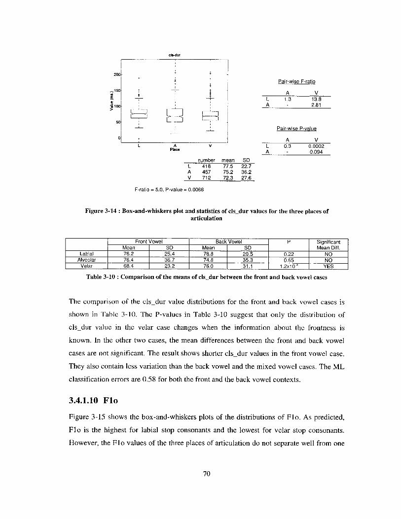
cis-dur
200!1
4i 47.150 ~ --i100
so
APlace
V
number meanL 418 77.5A 457 75.2V 712 72.3
F-ratio = 5.0, P-value = 0.0066
Figure 3-14 : Box-and-whiskers plot and statistics of cls_articulation
Pair-wise F-ratio
A VL 1.3 13.8A - 2.81
Pair-wise P-value
A VL 0.3 0.0002A - 0.094
SD22.736.227.6
dur values for the three places of
Front Vowel Back Vowel P SignificantMean SD Mean SD Mean Diff.
Labial 76.2 25.4 78.8 20.5 0.22 NOAlveolar 76.4 36.7 74.8 35.3 0.65 NO
Velar 68.4 23.2 76.0 31.1 1.2x10W YES
Table 3-10 : Comparison of the means of cls_dur between the front and back vowel cases
The comparison of the cls_dur value distributions for the front and back vowel cases is
shown in Table 3-10. The P-values in Table 3-10 suggest that only the distribution of
clsdur value in the velar case changes when the information about the frontness is
known. In the other two cases, the mean differences between the front and back vowel
cases are not significant. The result shows shorter cls_dur values in the front vowel case.
They also contain less variation than the back vowel and the mixed vowel cases. The ML
classification errors are 0.58 for both the front and the back vowel contexts.
3.4.1.10 Flo
Figure 3-15 shows the box-and-whiskers plots of the distributions of Flo. As predicted,
Flo is the highest for labial stop consonants and the lowest for velar stop consonants.
However, the Flo values of the three places of articulation do not separate well from one
70
L

another. The mean of Flo for the labial case is just slightly higher than the other two
cases, while, for the velar case, it is not much lower than the other two. The box parts of
the three groups overlap significantly. The means for the three places are 484.2 Hz, 461.9
Hz, and 444.7 Hz for labial, alveolar and velar stop consonants respectively. The F-ratio
is low. Thus, Flo is another acoustic attribute that should not separate the three places of
articulation well. The estimated probability of error based on ML classification is 0.62.
However, the pair-wise test shows that all of the P-values that are less than 0.01. That
means that, despite the small magnitude of the difference, this different is highly likely to
be caused from the place effect.
Flo
1200 -
1000
000 I IiPair-wise F-ratio800
A V
400-
200-
0- + +
L A VPlace
L 18.7 53.6A - 11.4
Pair-wise P-value
A VL 1.6x10-' 3.0x10-A - 0.0008
number mean SDL 1666 484.2 161.1A 1720 461.9 141.9V 1760 444.7 157.0
F-ratio = 28.7, P-value = 3.9 x 10-
Figure 3-15 Box-and-whiskers plot and statistics of Flo values for the three places of articulation
Front Vowel Back Vowel P SignificantMean SD Mean SD Mean Diff.
Labial 459.8 162.9 504.7 156.8 7.82x10 YESAlveolar 438.6 130.0 487.1 152.2 4.54x10' YES
Velar 414.9 145.4 474.6 163.3 1.22x10 YES
Table 3-11 : Comparison of the means of Flo between the front and back vowel cases
Table 3-11 compares the Flo values for the front and back vowel cases. It shows that the
mean values of Flo are significantly different between the two cases for all of the three
places of articulation. Across all of the three places, Flo for the front vowel case is
71

generally lower than for the back vowel case. Alveolar and velar stop consonants exhibit
less variation in the front vowel case than in the back vowel case, while the Flo variation
of labial stop consonants is rather similar for both the front and the back vowel cases. The
ML classification error for the front vowel case is 0.61, which is lower than the one for
the back vowel case, which is 0.64.
3.4.1.11 F2o
Figure 3-16 shows the box-and-whiskers plots of the distributions of F2o. As predicted,
F2o of the labial case is the lowest among the three cases. The standard deviation for the
velar case is 551.0 Hz, which is rather large compared to the standard deviations for the
labial and alveolar cases, which are 446.8 Hz and 354.6 Hz respectively. As mentioned
earlier, F2o values of velar stops are expected to be quite dependent on the frontness of
the adjacent vowel. Thus, this large variation when all of the vowels are mixed should be
expected. Despite this, the P-Value obtained from ANOVA is zero, which indicates that
the mean difference results from the place effect even when the vowels are mixed. Also,
all of the pair-wise P-values are smaller than 0.01 and the estimated probability of error
based on ML classification is 0.51.
F2o
3000 +
2500-Pair-wise F-ratio
2000 A
1500 -
1000-
SW -I
501
L A VPlace
L 585.7 519.4A - 12.98
Pair-wise P-value
A VL 0 0A - 0.0003
number mean SDL 1667 1445.8 446.8A 1718 1780.8 354.6V 1760 1837.6 551.0
F-ratio = 360.8, P-value = 0
Figure 3-16: Box-and-whiskers plot and statistics of F2o values for the three places of articulation
72
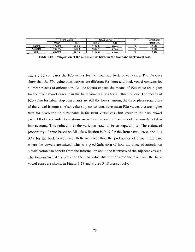
Front Vowel Back Vowel P SignificantMean SD Mean SD Mean Diff.
Labial 1778.9 364.9 1132.8 252.0 0 YESAlveolar 1967.6 328.3 1593.1 275.7 0 YES
Velar 2270.0 367.6 1416.2 349.7 0 YES
Table 3-12: Comparison of the means of F2o between the front and back vowel cases
Table 3-12 compares the F2o values for the front and back vowel cases. The P-values
show that the F2o value distributions are different for front and back vowel contexts for
all three places of articulation. As one should expect, the means of F2o value are higher
for the front vowel cases than the back vowels cases for all three places. The means of
F2o value for labial stop consonants are still the lowest among the three places regardless
of the vowel frontness. Also, velar stop consonants have mean F2o values that are higher
than for alveolar stop consonants in the front vowel case but lower in the back vowel
case. All of the standard variations are reduced when the frontness of the vowels is taken
into account. This reduction in the variation leads to better separability. The estimated
probability of error based on ML classification is 0.49 for the front vowel case, and it is
0.47 for the back vowel case. Both are lower than the probability of error in the case
where the vowels are mixed. This is a good indication of how the place of articulation
classification can benefit from the information about the frontness of the adjacent vowels.
The box-and-whiskers plots for the F2o value distributions for the front and the back
vowel cases are shown in Figure 3-17 and Figure 3-18 respectively.
73

F2o
A VPlace
number Mean SDL 799 1771.2 369.7A 897 1947.9 336.5V 885 2257.9 374.5
Pair-wise F-ratio
A VL 106.2 779.8A - 368.2
Pair-wise P-value
A VL 0 0A - 0
F-ratio = 420.7, P-value = 0
Figure 3-17 : Box-and-whiskers plot and statistics of F2o values where the vowels are front vowelsfor the three places of articulation
Pair-wise F-ratio
A VL 1242.5 349.5A - 135.4
Pair-wise P-value
A VL 0 0A - 0
number Mean SDL 886 1142.8 265.2A 821 1598.2 275.1V 870 1418.8 351.8
F-ratio = 503.3, P-value = 0
Figure 3-18 : Box-and-whiskers plot and statistics of F2o values where the vowels are back vowels forthe three places of articulation
74
3000
2500
2000
.01500
1000
500
0
4-
L
12o
2500
2000
500
0W
L APlace
V

3.4.1.12 F2b
Figure 3-19 shows the box-and-whiskers plots of the distributions of F2b. Similar to F2o,
F2b for the labial case is the lowest among the three cases as predicted. The means of F2b
for the three places of articulation are slightly higher than the ones for F2o. Compared to
F2o, the distributions of F2b in all three places of articulation contain larger standard
deviations. Thus, we expect F2b to be worse than F2o in separating the three places of
articulation. Nevertheless, the P-value from ANOVA is zero, which means that the mean
difference is the result of the place effect rather that the error. However, the pair-wise test
shows that not all of the pair-wise P-values are small enough to be significant. The P-
value between alveolar and velar stop consonants is 0.116 which is larger than 0.01. This
indicates that the mean values of F2b in the alveolar and the velar cases are not
significantly different. The difference observed is likely to be due to the error. The
estimated probability of error based on ML classification is 0.51.
F2b
5000 +
40M + _
3000 1 - Pair-wise F-ratio
2OW A V
1000-
0- -4-
-1000 -
-2000
L A VPlace
L 482.7 416.0A - 2.47
Pair-wise P-value
A VL 0 0A - 0.116
number mean SDL 1366 1460.9 708.7A 1225 1856.7 428.7V 1613 1887.7 861.4
F-ratio = 292.2, P-value = 0
Figure 3-19 Box-and-whiskers plot and statistics of F2b values for the three places of articulation
Front Vowel Back Vowel P SignificantMean SD Mean SD Mean Diff.
Labial 1755.6 825.2 1192.9 430.2 0 YESAlveolar 1979.0 445.6 1753.7 385.9 0 YES
Velar 2237.4 570.0 1555.8 948.7 0 YES
Table 3-13 : Comparison of the means of F2b between the front and back vowel cases
75

Table 3-13 compares the F2b values for the front and back vowel cases. Similar to the
F2o case, the P-values show that the F2b value distributions are different for both of the
cases for all three places of articulation. Again, as one should expect, the means of F2b
value are higher for the front vowel contexts than the back vowel contexts for all three
places. The means of F2b value for labial stop consonants are still the lowest among the
three places regardless of the vowel frontness. Velar stop consonants have mean F2o
values that are higher than for alveolar stop consonants in the front vowel case but lower
in the back vowel case. Unlike F2o, not all of the standard variations of F2b are reduced
when the frontness of the vowels are taken into account. The estimated probability of
error based on ML classification is 0.52 for the front vowel case, which is worse than the
error in the case where the vowels are mixed. It is 0.42 for the back vowel case, which is
noticeably better than 0.51 in the cases where the vowels are mixed.
3.4.1.13 F3o
Figure 3-20 shows the box-and-whiskers plots of the distributions of F3o. We can
observe that the F3o values of the three places of articulation do not separate well from
one another. The mean of F3o for the alveolar case is just slightly higher than the other
two cases. The distributions of the labial and the velar cases overlap each other and their
means are close to each other. The means for the three places are 2560 Hz, 2760 Hz, and
2590 Hz for labial, alveolar and velar stop consonants respectively. The estimated
probability of error based on ML classification is 0.56. The pair-wise test gives the P-
values that are all less than 0.01. That means that, despite the small magnitude of the
difference, this different is highly likely to be caused from the place effect.
76

F30
4=50 -4-
Pair-wise F-ratio
A VL 462.4 11.32A - 252.2
2000 ±
1500 + Pair-wise P-value
1000 A VL A V L 0 0.0008
PaeA -0
number mean SDL 1659 2555.9 287.9A 1718 2762.2 282.1V 1758 2592.0 349.4
F-ratio = 224.5, P-value = 0
Figure 3-20 Box-and-whiskers plot and statistics of F3o values for the three places of articulation
Front Vowel Back Vowel P SignificantMean SD Mean SD Mean Diff.
Labial 2599.5 303.5 2515.6 265.2 4.3x10-'u YESAlveolar 2844.5 254.2 2672.2 283.7 0 YESVelar 2769.6 333.6 2411.4 258.6 0 YES
Table 3-14: Comparison of the means of F3o between the front and back vowel cases
Table 3-14 compares the F3o values for the front and back vowel cases. It shows that the
mean values of F3o are significantly different between the two cases for all three places
of articulation. Across all three places, F3o for the front vowel case is generally higher
than for the back vowel case. Labial and velar stop consonants exhibit more variation in
the front vowel case than in the back vowel case, while the F3o variation of alveolar stop
consonants is smaller for both the front vowel case than the back vowel case. The ML
classification error for both of the cases is 0.54, which is lower than the one when the
vowels are mixed.
3.4.1.14 F3b
Figure 3-21 shows the box-and-whiskers plots of the distributions of F3b. Similar to F3o,
we can observe that the F3b values of the three places of articulation do not separate well
from one another. The mean of F3b for the alveolar case is just slightly higher than the
77

other two cases. The value distributions of the labial and the velar cases overlap each
other a lot and their means are close to each other. The means for the three places are
2540 Hz, 2830 Hz, and 2630 Hz for labial, alveolar and velar stop consonants
respectively. The estimated probability of error based on ML classification is 0.56, which
is the same as the one in the F3o case. The overall F-ratio is slightly lower than the F-
ratio in the F3o case. The pair-wise test gives the P-values that are all less than 0.01. That
means that, despite its small magnitude, this difference is highly likely to be caused from
the place effect.
5500
5000
4500
4000
F3500
.3000
2500
2000
1500
1000
500
*
-L
*
-
F3b
-I
I-
1-t
APlace
V
Pair-wise F-ratio
A VL 473.3 36.5A - 179.2
Pair-wise P-value
A VL 0 1.7x10A - 0
number mean SDL 1358 2542.7 581.2A 1222 2832.8 356.9V 1608 2633.7 512.1
F-ratio = 192.4, P-value = 0
Figure 3-21 Box-and-whiskers plot and statistics of F3b values for the three places of articulation
Front Vowel Back Vowel P SignificantMean SD Mean SD Mean Diff.
Labial 2572.9 638.7 2512.1 531.0 0.002 YESAlveolar 2879.5 399.4 2798.8 315.3 9.33x10 b YES
Velar 2840.1 413.6 2437.0 524.8 0 YES
Table 3-15 : Comparison of the means of F3b between the front and back vowel cases
Table 3-15 compares the F3b values for the front and back vowel cases. It shows that the
mean values of F3b are significantly different between the two cases for all three places
of articulation. Across all of the three places, F3b for the front vowel case is generally
higher than for the back vowel case, just like F3o. Labial and alveolar stop consonants
78
,

exhibit more variation in the front vowel case than in the back vowel case, while the
opposite is true for the velar stop consonants. The ML classification error for the front
vowel case is 0.57 and 0.54 for the back vowel case. Only for the latter case is the error
better than when the vowels are mixed.
3.4.1.15 dF2
Figure 3-22 shows the box-and-whiskers plots of the dF2 distributions regardless of the
frontness of the adjacent vowels. Despite the mixing of front and back vowels, the plots
show reasonable separability among the three places of articulations. The F-ratio is high
and the overall P-value, as well as all of the pair-wise P-values, is zero, indicating that the
mean differences among all groups are due to the place effect rather than the error within
group. And, as expected, most of the time dF2 values for labial stop consonants are
negative, which means that the second formant frequency goes up as we move toward the
middle of the vowel. The means of dF2 value for the three places of articulation are
significantly different between the front and the back vowel cases as shown in Table 3-16
and in the box-and-whiskers plots in Figure 3-23 and Figure 3-24. In both the front and
the back vowel cases, labial stop consonants have dF2 values that are large negative
numbers. The dF2 mean is more negative for the front vowel case, indicating the larger
frequency interval that the second formant frequency needs to climb. For alveolar stop
consonants, dF2 mean is a small negative number for the front vowel case, while it is
positive for the back vowel case. The second formant frequencies in the velar case tend to
go down as they move from the stop consonant into the vowel. This is reflected in the
positive dF2 means for both the front and back vowel cases. The second formant
frequencies do not move as much for the front vowel case as they do in the back vowel
case. Despite the higher standard deviations for all three places in front vowel contexts,
the value distribution of velar stop consonants is well separated from the other two cases
due to the large mean difference. However, this is not the case for the back vowel
context, in which the three places do not seem to be separated as well as for the front
vowel context. The estimated probability of error based on ML classification is 0.35 for
the front vowel case, which can be considered to be rather good, compared to 0.44 for the
79

mixed vowel case. The probability of error for the back vowel case is 0.45, which is close
to the mixed vowel case.
dF2
600
400 --
200 Pair-wise F-ratio
A V-200 L 1096.2 2448.8.WA - 261.5
4600
-800 Pair-wise P-value-1000
A VL A VPlace L 0 0
number mean SDL 1664 -149.7 183.1A 1718 27.5 135.1V 1758 94.6 111.1
A - 0
F-ratio = 1354.1, P-value = 0
Figure 3-22 Box-and-whiskers plot and statistics of dF2 values for the three places of articulation
Front Vowel Back Vowel P SignificantMean SD Mean SD Mean Diff.
Labial -206.4 218.7 -101.0 123.9 0 YESAlveolar -47.3 108.6 117.4 102.1 0 YES
Velar 106.9 113.0 82.8 107.9 3.29x10~' YES
Table 3-16: Comparison of the means of dF2 between the front and back vowel cases
80

V
number mean SDL 798 -205.4 217.7A 896 -44.5 110.0V 890 106.2 113.1
Pair-wise F-ratio
dF2
~ *
-W
F-ratio = 929.2, P-value = 0
Figure 3-23 : Box-and-whiskers plot and statistics of dF2 values where the vowels are front vowelsfor the three places of articulation
dF2
*
-A -
L VAPlace
Pair-wise F-ratio
A VL 1251.6 1134.8A - 18.39
Pair-wise P-value
A VL 0 0A - 1.9X10 5
number mean SDL 868 -100.9 123.8A 821 105.5 115.4V 868 82.7 107.7
F-ratio = 842.1, P-value = 0
Figure 3-24: Box-and-whiskers plot and statistics of dF2 values where the vowels are back vowels forthe three places of articulation
81
A VL 407.44 1489.5A - 827.0
Pair-wise P-value
A VL 0 0A - 0
400
200
0
-200
-400
-800
-800
-1000
-1200
L APlace
800
400
200
0I0
-200
-400
-800

3.4.1.16 dF2b
Figure 3-25 shows the box-and-whiskers plots of the dF2b distributions regardless of the
frontness of the adjacent vowels. Visually, dF2b does not show as much separability as
dF2. The means of dF2b are close to the means of dF2 in all of the places of articulation,
but the standard deviations in dF2b are a lot larger than the ones in dF2. Despite that, the
overall P-value, as well as all of the pair-wise P-values, is less than 0.01, indicating that
the mean differences among all groups are due to the place effect rather than the error
within group, just as in the dF2 case. Also, as expected, most of the time dF2 values for
labial stop consonants are negative. The means of dF2 for labial and alveolar stop
consonants are significantly different between the front and the back vowel cases, but not
for the velar case, as shown in Table 3-17. Although the mean values of dF2b for velar
stop consonants for the front and the back vowel cases follow the same trend as we
observed when the vowel with different frontness are separated in the dF2 case, the
difference between these means are more likely to come from the within group error. For
labial stop consonants, in both the front and the back vowel cases, the means of dF2b are
large negative numbers similar to dF2. The dF2b mean is more negative for the front
vowel case. For alveolar stop consonants, the dF2b mean is a small negative number for
the front vowel case, while it is positive for the back vowel case. The estimated
probability of error based on ML classification when the vowels are mixed is 0.53, while
it is just 0.48 for the front vowel case. Similar to the dF2 case, this is due to the fact that
dF2b of velars stands out from dF2b of the other two places for front vowel. However,
the error probability is 0.55 for the back vowel case.
82

dF2b
1500
1000- *Pair-wise F-ratio500
A V0- L 444.4 854.3
A - 43.1~-500 +1-1500 Pair-wise P-value
-2000 A VL A V L 0 0
A - 6.3x10~"
number mean SDL 1358 -140.4 368.3A 1225 44.3 220.9V 1605 91.4 250.1
F-ratio = 486.8, P-value = 0
Figure 3-25 Box-and-whiskers plot and statistics of dF2b values for the three places of articulation
Front Vowel Back Vowel P SignificantMean SD Mean SD Mean Diff.
Labial -207.1 426.1 -82.6 297.0 0 YESAlveolar -8.1 217.1 99.2 217.9 0 YES
Velar 100.1 225.8 85.7 272.1 0.13 NO
Table 3-17 : Comparison of the means of dF2b between the front and back vowel cases
3.4.1.17 dF3
Figure 3-26 shows the box-and-whiskers plots of the dF3 distributions. Alveolar stop
consonants can be separated well from the labial stop consonants for this measure. Their
box parts of the plots, each of which is corresponding to half of the total samples
belonging to that place, do not overlap. The majority of dF3 values for labial stop
consonants are negative, which means that most of the time the third formant frequencies
increase when they move from labial stop consonants to the adjacent vowels. The dF3
mean for labial stop consonants is a large negative number. The mean for the velar case is
slightly more than the labial case. The mean for the alveolar case is the highest, yet still it
is a negative number. However, from the distribution, the upward and downward
movements are mixed more equally in the alveolar case, and the corresponding mean
value is close to zero. The overall P-value and all of the pair-wise P-values are zeros,
83

indicating that the difference in the dF3 means of the three places of articulation is due to
the place effect. The estimated probability of error based on ML classification is 0.52.
dF3
200- Pair-wise F-ratio
A V
400 -
-400-
-800 -*
L A VPlace
L 975.2 247.2A - 263.9
Pair-wise P-value
A VL 0 0A - 0
number mean SDL 1663 -145.0 149.1A 1718 -4.9 111.9V 1757 -71.1 129.8
F-ratio = 495.2, P-value = 0
Figure 3-26 Box-and-whiskers plot and statistics of dF3 values for the three places of articulation
Front Vowel Back Vowel P SignificantMean SD Mean SD Mean Diff.
Labial -182.0 165.4 -111.1 123.4 0 YESAlveolar -27.9 110.1 21.5 108.4 0 YES
Velar -40.6 130.7 -102.4 121.2 0 YES
Table 3-18 : Comparison of the means of dF3 between the front and back vowel cases
Table 3-18 shows the comparison between dF3 values in the front and the back vowel
cases. All of the P-values are zeros, indicating that the frontness of the vowels affects the
dF3 value distribution for all three places of articulation. Regardless of the vowels, labial
stop consonants show large negative means. The dF3 mean in the front vowel case for
alveolar stop consonant shows a small upward movement into the adjacent vowels, while
the mean for the back vowel case shows a small downward movement. For velar stop
consonants, the mean values of dF3 show a larger upward movement into the back
vowels than the upward movement into the front vowels. The probability of error based
on ML classification is 0.51 for the front vowel case and 0.52 for the back vowel case.
84
-j

3.4.1.18 dF3b
Figure 3-27 shows the box-and-whiskers plots of the dF3b distributions. Alveolar stop
consonants can be separated well from the labial stop consonants, as in the dF3 case.
Their box parts of the plots, each of which is corresponding to half of the total samples
belonging to that place, do not overlap. However, the standard deviations of the three
places of articulation are larger for dF3b than for dF3. We can also observe a large
number of data points that lie outside the value ranges of their whiskers. The means of
dF3b are close to the means of dF3 with the corresponding places, except for that the
mean for alveolar stop consonants show a small downward movement instead of a small
upward one. The overall P-value and all of the pair-wise P-values are zeros, indicating
that the difference in the dF3b means of the three places of articulation is due to the place
effect. The estimated probability of error based on ML classification is 0.52.
dF3b
1500
1000Pair-wise F-ratio
____ IA VL 414.0 114.8
-500 A - 158.5
-1000
-1500 Pair-wise P-value-2000 A V
+_ _ _ __ _ _ _ A VL A V L 0 0
Pac A - 0
number mean SDL 1359 -140.7 432.7A 1222 37.3 195.4V 1600 -50.8 280.8
F-ratio = 227.1, P-value = 0
Figure 3-27: Box-and-whiskers plot and statistics of dF3b values for the three places of articulation
Front Vowel Back Vowel P SignificantMean SD Mean SD Mean Diff.
Labial -165.6 393.5 -120.2 470.3 0.002 YESAlveolar 4.2 212.3 69.6 176.1 1.01X10⁻¹ YES
Velar -21.9 275.2 -78.3 282.6 7.46x10- YES
Table 3-19: Comparison of the means of dF3b between the front and back vowel cases
85

Table 3-19 shows the comparison between dF3b values in the front and the back vowel
cases. All of the P-values are zero, indicating that the frontness of the vowels affects the
dF3b value distribution for all three places of articulation. Regardless of the vowels,
labial stop consonants show large negative means, while small positive values are shown
for the alveolar case. For velar stop consonants, the mean values of dF3b show a larger
downward movement into the back vowels than the downward movement into the front
vowels, as in the dF3 case. The probability of error based on ML classification is 0.55 for
the front vowel case and 0.48 for the back vowel case. The former is worse than the case
where the vowels are mixed, while the latter is better.
3.4.1.19 F3o-F2o
Figure 3-28 shows the box-and-whiskers plots of the F3o-F2o distributions. As expected,
on average, F3o-F2o is the smallest for the velar case. The average space between the
second and third formant frequencies at the voicing onset or offset of the adjacent vowels
is 753 Hz. The mean of F3o-F2o is the largest for the labial case, which is 1110 Hz, while
it is 980 Hz for the alveolar case. The IQR of F3o-F2o in the alveolar case is in the range
of the IQR of F3o-F2o in the labial case completely. For the velar case, its IQR overlaps
partially with the IQR in the labial case. The overall P-value and all of the pair-wise P-
values are zeros, indicating that the difference in the F3o-F2o means of the three places
of articulation is due to the place effect. The estimated probability of error based on ML
classification is 0.51.
Table 3-20 shows the comparison between F3o-F2o values in the front and the back
vowel cases. All of the P-values are zero, indicating that the frontness of the vowels
affects the F3o-F2o value distribution for all three places of articulation. In general, the
gap between the second and the third formant frequencies is smaller in the front vowel
case than in the back vowel case. For both the front vowel and the back vowel cases, the
standard deviations are smaller than when the vowels are mixed, except for alveolar stop
consonants in the back vowel case, where the standard deviation is slightly higher. The
probability of error based on ML classification is 0.49 for the front vowel case, which is
86

better than the one in the case where the vowels are mixed. It is 0.51 for the back vowel
case, which is similar to the case where the vowels are mixed.
F3o-F2o
2500
2000 Pair-wise F-ratio
± I A VL 114.0 633.1
_ I A - 332.01000E
Pair-wise P-value
0- A VL A V L 0 0
Place A - 0Number mean SD
L 1664 1107.5 393.7A 1717 980.3 295.9V 1759 752.8 429.0
F-ratio = 391.5, P-value = 0
Figure 3-28 : Box-and-whiskers plot and statistics of F3o-F2o values for the three places ofarticulation
Front Vowel Back Vowel P SignificantMean SD Mean SD Mean Diff.
Labial 816.9 241.3 1373.6 318.7 0 YESAlveolar 885.6 246.7 1076.8 311.0 0 YES
Velar 506.3 324.2 989.5 393.0 0 YES
Table 3-20 : Comparison of the means of F3o-F2o between the front and back vowel cases
3.4.1.20 F3b-F2b
Figure 3-29 shows the box-and-whiskers plots of the F3b-F2b distributions. Again, as
expected, the mean of F3b-F2b is the smallest for the velar case. However, similar to
what we have found for the acoustic attributes that are measured at the release burst
compared to its counterpart at the voicing onset or offset so far, the standard deviations of
F3b-F2b are larger than the ones of F3o-F2o for all of the places of articulation. The
means of F3b-F2b are slightly smaller than F3o-F2o. ANOVA shows that the difference
in means among the three places of articulation is significant. The pair-wise test also
87
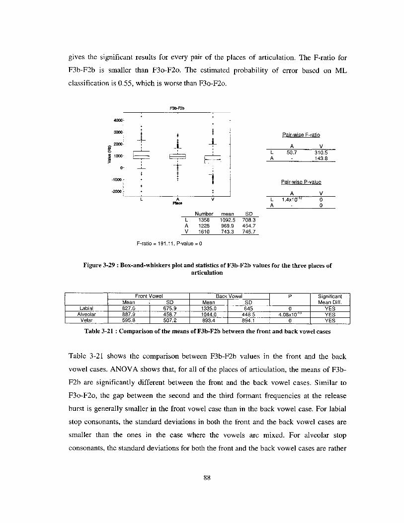
gives the significant results for every pair of the places of articulation. The F-ratio for
F3b-F2b is smaller than F3o-F2o. The estimated probability of error based on ML
classification is 0.55, which is worse than F3o-F2o.
F3b-F2b
4M00
3M00 Pair-wise F-ratio
2000 A V
L 50.7 310.5A - 143.8
0-
-1000 Pair-wise P-value
-2000 - + A V
L A V L 1.4x10' 0A - 0
Number mean SDL 1358 1092.5 708.3A 1225 969.9 454.7V 1610 743.3 745.7
F-ratio= 191.11, P-value = 0
Figure 3-29 Box-and-whiskers plot and statistics of F3b-F2b values for the three places ofarticulation
Front Vowel Back Vowel P SignificantMean SD Mean SD Mean Diff.
Labial 827.0 675.9 1335.0 645 0 YESAlveolar 887.9 458.7 1044.0 448.5 4.08x10* YES
Velar 595.8 507.2 893.4 894.1 0 YES
Table 3-21 : Comparison of the means of F3b-F2b between the front and back vowel cases
Table 3-21 shows the comparison between F3b-F2b values in the front and the back
vowel cases. ANOVA shows that, for all of the places of articulation, the means of F3b-
F2b are significantly different between the front and the back vowel cases. Similar to
F3o-F2o, the gap between the second and the third formant frequencies at the release
burst is generally smaller in the front vowel case than in the back vowel case. For labial
stop consonants, the standard deviations in both the front and the back vowel cases are
smaller than the ones in the case where the vowels are mixed. For alveolar stop
consonants, the standard deviations for both the front and the back vowel cases are rather
88

similar and they are also rather similar to the ones in the case where the vowels are
mixed. For velar stop consonants, the front vowel case shows a smaller standard
deviation than the one in the case where the vowels are mixed, while it is larger for the
back vowel case. The probability of error based on ML classification is 0.56 for the front
vowel case, which is slightly worse than the one in the case where the vowels are mixed.
And, it is 0.52 for the back vowel case, which is better.
3.4.1.21 cgFlOa
The box-and-whiskers plots of the values of cgFlOa are shown in Figure 3-30. As
predicted, the mean value for cgFlOa is the highest for alveolar stops at 2700Hz,
followed by the mean value of velar stops at 1730Hz. Labial stops have the lowest mean
for cgFlOa at 665Hz. From the box-and-whiskers plots, we can observe that cgFlOa for
the labial case is well separated from the other two cases and the labial case also shows a
smaller standard deviation. Although there are some overlaps between the IQRs of the
alveolar and the velar cases, the means for the two cases are rather far apart. This
attribute should be able to perform well in classifying the place of articulation. From
ANOVA, the overall P-value obtained is 0 as well as all of the pair-wise P-values. This
indicates that the differences in means of cgFlOa for the three places of articulation are
statistically significant. The estimated probability of error based on ML classification is
0.30.
Table 3-22 compares the means of cgFlOa for each place of articulation between the front
and the back vowel cases. The result shows that the frontness of the adjacent vowel does
not statistically affect the value of cgFlOa for the alveolar case while it does in the other
two places of articulation. The difference between the means of cgF1Oa for velar stops in
the front and the back vowel cases are quite large. From this finding, one could expect
that the estimate of a probability of error would be different if we know the information
of the frontness of the vowel. In the front vowel case, the means of cgF1Oa for the velar
and alveolar stops lie closer to each other than when the vowels are mixed, while the
cgFlOa values for labials does not overlap with the other two types of stop significantly
regardless of frontness information. This results in the larger degree of overlapping
89

among the distributions of the three places. On the contrary, the degree of overlapping is
smaller in the back vowel case where the mean of cgFlOa for alveolars moves up and the
one for the velar case moves down. The standard deviations in the front vowel case are
bigger than when we do not use the frontness information, while in the back vowel case,
it is smaller. This leads to the increase in the estimated probability of error based on ML
classification for the front vowel case, which is 0.39, and the reduction to 0.22 in the back
vowel case, which is the smallest estimated probability of error among the attributes
studied so far.
cgFIOa
6000-
Pair-wise F-ratio4000
A VL 2015.9 1695.2A - 360.0
2000
1000 Pair-wise P-value
0 ;A VL L 0 0
Place A - 0
number mean SDL 946 665.1 372.4A 775 2704.8 1345.4V 901 1726.1 711.0
F-ratio 1188.3, P-value = 0
Figure 3-30: Box-and-whiskers plot and statistics of cgFlOa values for the three places of articulation
Front Vowel Back Vowel P SignificantMean SD Mean SD Mean Diff.
Labial 737.1 429.7 604.8 290.9 6.9x10- YESAlveolar 2571.8 1469.0 2800.0 1242.5 0.02 NO
Velar 2099.3 761.0 1371.1 428.9 0 YES
Table 3-22: Comparison of the means of cgF10a between the front and back vowel cases
3.4.1.22 egF20a
The box-and-whiskers plots of the values of cgF20a are shown in Figure 3-31. The
distribution of cgF20a for the three places of articulation looks similar to the one of
90

cgFlOa. The differences among the means of cgF20a for the three places are statistically
significant. Compared to cgFlOa, cgF20a contains more variation in its values, as
observed from the larger standard deviations, resulting in a larger overlapping among the
values of the three places. The estimated probability of error based on ML classification
is 0.31.
cgF20a
0
0
0
L APlace
V
Pair-wise F-ratio
A VL 2011.8 951.5A - 593.0
Pair-wise P-value
A VL 0 0A - 0
Figure 3-31:
number mean SDL 949 765.1 451.0A 775 2986.0 1444.3V 901 1643.4 749.7
F-ratio = 1200.7, P-value = 0
Box-and-whiskers plot and statistics of cgF20a values for the three places of articulation
Front Vowel Back Vowel P SignificantMean SD Mean SD Mean Diff.
Labial 879.7 524.4 660.0 333.4 2.6x10⁴ YESAlveolar 2932.6 1602.5 3024.2 1320.3 0.38 NO
Velar 2085.0 790.1 1229.2 386.9 0 YES
Table 3-23: Comparison of the means of cgF20a between the front and back vowel cases
Table 3-23 compares the means of cgF20a for each place of articulation between the front
and the back vowel cases. The result shows that the frontness of the adjacent vowel does
not statistically affect the value of cgF20a for the alveolar case while it does for the other
two places of articulation. The finding is similar to cgFlOa. The standard deviations in
the front vowel case are larger than when we do not use the frontness information while
in the back vowel case, it is smaller. The means of the alveolar stops and the velar stops
are closer to each other in the front vowel context than in the case the vowels are mixed,
while for the back vowel context, the means are further apart. This results in the
91
60
040M
~30C
200
100
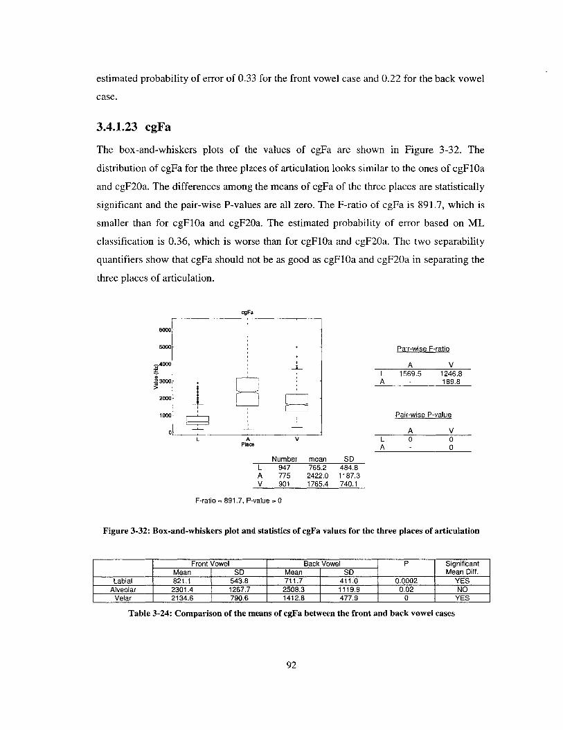
estimated probability of error of 0.33 for the front vowel case and 0.22 for the back vowel
case.
3.4.1.23 cgFa
The box-and-whiskers plots of the values of cgFa are shown in Figure 3-32. The
distribution of cgFa for the three places of articulation looks similar to the ones of cgFlOa
and cgF20a. The differences among the means of cgFa of the three places are statistically
significant and the pair-wise P-values are all zero. The F-ratio of cgFa is 891.7, which is
smaller than for cgFlOa and cgF20a. The estimated probability of error based on ML
classification is 0.36, which is worse than for cgFlOa and cgF20a. The two separability
quantifiers show that cgFa should not be as good as cgFlOa and cgF20a in separating the
three places of articulation.
cgFa
6000-
5000 +
_4O000-3000 -
3000
0000
0L A
PlaceV
Pair-wise F-ratio
A VL 1569.5 1246.8A - 189.8
Pair-wise P-value
A VL 0 0A - 0
Number mean SDL 947 765.2 484.8A 775 2422.0 1187.3V 901 1765.4 740.1
F-ratio = 891.7, P-value = 0
Figure 3-32: Box-and-whiskers plot and statistics of cgFa values for the three places of articulation
Front Vowel Back Vowel P SignificantMean SD Mean SID Mean Diff.
Labial 821.1 543.8 711.7 411.0 0.0002 YESAlveolar 2301.4 1267.7 2508.3 1119.9 0.02 NO
Velar 2134.6 790.6 1412.8 477.9 0 YES
Table 3-24: Comparison of the means of cgFa between the front and back vowel cases
92

Table 3-24 compares the means of cgFa for each place of articulation for the front and the
back vowel cases. The result shows that the frontness of the adjacent vowel does not
statistically affect the value of cgFa for alveolars while it does for the other two places of
articulation. The finding is similar to that for cgFl0a and cgF20a. The standard
deviations for the front vowel case are bigger than when we do not use the frontness
information, while for back vowel context, it is smaller, especially for velars. The means
of the alveolar stops and the velar stops are closer to each other in the front vowel case
than in the case where the vowels are mixed, while for back vowels, the means are further
apart. The labial stop consonants are well separated from the other two, as they are in the
cgFl0a and cgF20a cases. This results in the estimated probability of error of 0.39 for
front vowel context and 0.29 for the back vowel context.
3.4.2 Comparison of Each Acoustic Attribute's Discriminating
Property
Although it has been shown by the significance test of the mean difference that all of the
acoustic attributes introduced in this chapter contain some level of ability to separate the
three places of articulation, we would like to evaluate the relative ability of each of the
acoustic attributes to separate the three places. As mentioned, the F-ratio for each of the
acoustic attributes is the ratio between the amount of the variation that appear in the
values of that acoustic attribute that is caused by the place effect to the amount of the
variation caused by the within-place error. Therefore, an acoustic attribute that can be
used to separate among the three places of articulation well should have a high F-ratio,
which means that the place effect is much larger than the within-place error, while an
acoustic attribute with a small F-ratio should not be able to do well. Thus, F-ratio is used
here as one measure to compare the discriminating property of each acoustic attribute.
Another quantity that is used for such a comparison is the estimated maximum likelihood
classification error probability. Obviously, a small error probability shows good
separability, while a big one shows poor separability.
Table 3-25 and Table 3-26 summarize the F-ratios, normalized by the number of data
points used for each acoustic attribute, as mentioned in section 3.4, and the maximum
93

likelihood classification error probabilities of every acoustic attribute. The normalized F-
ratios in Table 3-25 are sorted in descending order, while the error probabilities in Table
3-26 are sorted in ascending order. Both quantifiers agree on the acoustic attributes that
do not separate the three places of articulation well. The bottom six acoustic attributes in
both tables include clsdur, VOT, Flo, F3b-F2b, F3o, and F3b. In general, the acoustic
attributes that are used for capturing the spectral shape of the release burst are closer to
the top of both tables than the acoustic attributes that are used to capture the formant
structure around the stop consonants and the temporal acoustic attributes. The bottom six
acoustic attributes consist of only the formant-related acoustic attributes and both of the
temporal cues. In both tables, dF2 is the only formant-related acoustic attribute that has a
high normalized F-ratio and a low error probability. The acoustic attributes that show
good separability in both tables include cgFlOa, cgF20a, cgFa, Av-Ahi, Ahi-A23, Av-
Amax23, and dF2. These acoustic attributes include all of the ones that describe the
energy distribution in the time interval between the release burst and the voicing onset of
the following vowel, as well as all of the ones that describe the spectral shape of the
release burst in relation to the vowel amplitude at the first formant frequency. The
acoustic attributes that describe the spectral amplitude in certain frequency ranges
relative to the vowel amplitude in the same frequency ranges, which are Avhi-Ahi, Av3-
A3, and Av2-A2, do not provide as good discriminating property as the other burst-
related acoustic attributes.
However, in order for the F-ratio to represent the separability among the three groups
well, the standard deviations of the three groups should be rather similar. Although, it
was shown in [Lindman, 1974] that the F-ratio was quite robust to the difference of the
group standard deviations, it is worth noting that some of the acoustic attributes have
large differences in the standard deviations among the three places, as shown in the
associated results in section 3.4.1. These acoustic attributes include cgFlOa, cgF20a,
cgFa, and Ehi-E23. For these acoustic attributes, it might be more appropriate to
determine their abilities to separate the three places by the ML classification error
probabilities. Although for the first three attributes, the trends of both the F-ratios and the
ML classification errors are consistent, Ehi-E23 shows a very low classification error
94

probability while it does not contain a very high F-ratio in comparison to other acoustic
attributes that also show low classification error probabilities.
Acoustic Attribute Name Normalized F-ratiocgF20a 0.46cgF1Oa 0.45CgFa 0.34Av-Ahi 0.32
Av-Amax23 0.27dF2 0.24
Ahi-A23 0.23Ehi-E23 0.21Av2-A2 0.12Av3-A3 0.12
dF2b 0.12Avhi Ahi 0.12
dF3 0.10F3o-F2o 0.08F2o 0.07F2b 0.07
dF3b 0.05F3b 0.05
F3b-F2b 0.05F3o 0.04vot 0.03Flo 0.01
Cis dur 0.00
Table 3-25: normalized F-ratios of every acoustic attribute, sorted in descending order
Acoustic Attribute Name ML Classification ErrorcgF10a 0.30cgF20a 0.31Ehi-E23 0.34cgFa 0.36Av-Ahi 0.44
Ahi-A23 0.44dF2 0.44
Av-Amax23 0.45Avhi Ahi 0.51
F2o 0.51F2b 0.51
F3o F2o 0.51dF3 0.52dF3b 0.52
Av3-A3 0.53Av2-A2 0.53
dF2b 0.53F3b-F2b 0.55
F3o 0.56F3b 0.56vot 0.59
Cis dur 0.59Flo 0.62
Table 3-26: Maximum likelihood classification error of every acoustic attribute, sorted in ascendingorder
95

100%
8 90% --- - --- - - -- - - -- --- ----- ---- -- - -- ----- --- -- ---- ---- F ra i0% - -0/- -- - - - -------- - - -- -------- --- F-ratio -
-gj 70% -- -- - - --- ------------ --- - --- - --- - - --- -
E 60% - - ------------------------- E-1-P(err) -50% - ---- - -- - - - ---- --- ------- --- - ----
30 5Q/----------------------------- ------------ ------------E 40% --- ---- --------- -- ---
0 30% ---- ---- -- --- ------ --- --------
10% ------------ ----- ----------- ------------0% . ,
0rt %
(U Cz C U ( C\1 Cf) CV) 0 0 M0 Cf) C'J cr) .0 -0 .0 f 0 ~ - 0
0) 0) E= 0 > > 01o W< X- E Cf) <oUJ < <U- U
Acoustic attribute
Figure 3-33: Comparison between the F-ratios and the ML classification error probabilities, P(err),of all of the acoustic attributes. Note that, the ML classification error probabilities are plotted in theform of 1-P(err). Both are scaled so that the maximal values are at 100%, while the minimal values
are at 0%.
Figure 3-33 compares the ability to separate the three places of articulation of all of the
acoustic attributes determined by both quantifiers. It can be observed from the figure that
both the noralized F-ratio and the ML classification error probability generally agree,
except for Ehi-E23, as mentioned earlier.
3.4.3 Correlation Analysis
Redundancy in the information contained in all of the acoustic attributes could hurt the
classification performance, cause unnecessary computational cost, and undermine some
statistical analyses to be performed such as the discriminant analysis. Therefore, we wish
to identify the acoustic attributes that are highly correlated with other acoustic attributes
and use the findings to guide the selection of acoustic attribute subsets. These attributes
will then be used for further classification experiments and their corresponding analyses.
Two acoustic attributes are considered to be perfectly correlated with each other when,
for every token, one can predict the value of one acoustic attribute accurately knowing
the value of the other acoustic attribute of the same token. They are uncorrelated when
the value of one acoustic attribute does not yield any information in predicting the value
of the other attribute. We wish to determine where the correlation between each of the
possible pairs of acoustic attributes lies in between these two extreme cases. A quantity
96

commonly used for this purpose is the square of the correlation coefficient (p2 ). The
values of p2 between pairs of acoustic attributes were calculated from the tokens for
which both acoustic attributes are applicable. Any values of the acoustic attributes that lie
farther than five times the standard deviation from their means were considered outliers
and removed prior to calculating the corresponding correlation coefficients.
The acoustic attribute pairs whose P2 are higher than 0.80 across different contexts for
both CV and VC tokens are listed in Table 3-27 and Table 3-28.
Context Highly Correlated Attribute Pairs (p > 0.80)All (Av3-A3 & Av2-A2), (cgF1 Oa & cgF20a)
Voiced Stop (Av3-A3 & Av2-A2), (F2o & F2b), (F3o & F3b), (cgF1 Oa & cgF20a)Voiceless Stop (Av3-A3 & Av2-A2), (cgF1 Oa & cgF20a)
Front Vowel (Av3-A3 & Av2-A2)Back Vowel (Av3-A3 & Av2-A2), (cgF1Oa & cgF20a), (cgF1Oa & cgFa)
Voiced Stop + Front Vowel (Av3-A3 & Av2-A2), (F2o & F2b), (F3o & F3b)Voiced Stop + Back Vowel (Av3-A3 & Av2-A2), (F2o & F2b), (F3o & F3b), (cgF1Oa & cgF20a), (cgF1Oa &
cgFa), (cgF20a & cgFa)Voiceless Stop + Front Vowel (Av3-A3 & Av2-A2)Voiceless Stop + Back Vowel (Av3-A3 & Av2-A2), (cg F1 a & cg F20a)
Table 3-27: Highly correlated attribute pairs (p2 > 0.80) across different CV contexts
Context Highly Correlated Attribute Pairs (p2 > 0.80)All (Av3-A3 & Av2-A2)
Voiced Stop (Av3-A3 & Av2-A2)Voiceless Stop (Av3-A3 & Av2-A2)
Front Vowel (Av3-A3 & Av2-A2)Back Vowel (Av3-A3 & Av2-A2)
Front Vowel + Voiced Stop (Av3-A3 & Av2-A2)Back Vowel + Voiced Stop (Av3-A3 & Av2-A2)
Front Vowel + Voiceless Stop (Av3-A3 & Av2-A2)Back Vowel + Voiceless Stop (Av3-A3 & Av2-A2)
Table 3-28: Highly correlated attribute pairs (p2 > 0.80) across different VC contexts
In every case, the attributes Av3-A3 and Av2-A2 are highly correlated. Their p are
always higher than 0.90, which are always the highest among any pairs of attributes.
Most of the time the values of Av3-A3 and Av2-A2 vary in a similar fashion among all
of the tokens. Both Av3-A3 and Av2-A2 are intended to capture a similar type of
information, which is the amplitude of the release burst relative to the amplitude of the
adjacent vowel in the same frequency region. However, the frequency ranges used in the
two attributes are different. The correlation result indicates that the difference in the
frequency ranges for the two attributes does not add much additional information.
97
Therefore, using only one of them in the classification should suffice. It is left to
determine which one of them should be selected to achieve better classification results. In
the VC case, only this pair of attributes is strongly correlated.
The second and third formant frequencies measured at the voicing onset of the vowels are
highly correlated with their counterparts measured at the release burst in almost every
case that the attribute values obtained from voiced stops are analyzed separately from the
ones from voiceless stops in CV tokens. However, they are not strongly correlated in the
voiceless cases. This is not surprising since it has been shown earlier that the VOTs of
voiced stops are significantly shorter than the ones of voiceless stops. So, the time points
where the voicings of the vowels start are closer to the release burst and this results in
more similar formant frequencies between the two time points. However, the correlations
are not as strong as the ones between Av3-A3 and Av2-A2.
In some cases, cgFlOa, cgF20a and cgFa are highly correlated with one another, although
the correlations are not as strong as the two cases mentioned above. These correlations
are expected since in some of the CV tokens whose VOT's are short, the portion of the
speech signal used for calculating these three acoustic attributes are the same due to the
reason mentioned earlier in this chapter.
As mentioned, the attributes investigated in this thesis are placed into four categories
depending on whether the attributes are intended to capture the spectral shape of the
release burst, the formant frequency structure, the energy concentration of the signal
between the burst and the voicing onset of the vowel, or the timing of the signal. From
the correlation analysis, we have found that there are no cross-category highly correlated
acoustic attributes.
3.5 Chapter Summary
In this chapter, the acoustic attributes used in this thesis were introduced along with their
descriptions and related measurement techniques. The time points at the release burst and
98

at the voicing onset or offset of the adjacent vowel were marked manually prior to the
measurement of the acoustic attributes. For consistency across the manually time marking
process, the time points marked as the voicing onset and offset were refined by picking
the places where the rate of change of the low-frequency energy around the originally
marked points was maximal. The distributions of the values of each acoustic attribute
were shown for all three places of articulation. Box-and-whiskers plots were used to
provide visual indication of how well each acoustic attribute can separate the three places
of articulation. The significance of the mean differences among the three places of
articulation was tested. The results showed that all of the acoustic attributes introduced
here had significant mean difference among the three places of articulation. The
information about vowel frontness altered the separabilities among the three places of
articulation of the acoustic attributes. Some acoustic attributes could separate the three
places better if the frontness of the vowels were known. The ability to separate the three
places of articulation of the acoustic attributes were compared by means of their F-ratios
and maximum likelihood classification error probabilities. It was shown that both
temporal attributes along with some of the formant-related attributes were poor in
separating the three places of articulation, while all of the acoustic attributes that capture
the spectral energy concentration after the release burst and some of the burst-related
attributes were among the best acoustic attributes for discriminating among the three
places. In general, the acoustic attributes that capture the spectral shape of the release
burst did better than the acoustic attributes that capture the formant structure. Finally, a
correlation analysis was performed in order to uncover possible redundant information
among the acoustic attributes. Some highly correlated acoustic attributes were identified
within various frontness and voicing contexts. However, there was no evidence of highly
correlated acoustic attributes cross categories.
99

This page is intentionally left blank.
100

Chapter 4
Classification Experiments
In the last chapter, the acoustic attributes involved in this research were introduced. Their
discriminating properties were investigated by observing the statistics obtained from the
distribution of each attribute. The estimated ML classification errors and the F-ratios
show how well each individual attribute can distinguish among the three places of
articulation. In this chapter, we will perform classification experiments based on subsets
of attributes introduced in the last chapter. The purpose of these classification
experiments is to evaluate the classification performance when subsets of these acoustic
attributes are used as "feature vectors" input to a simple statistical classifier. Positive
results will show that the acoustic attributes introduced in this study are appropriate for
determining the place of articulation features in the feature bundle for a stop consonant
segment, while negative results will provide more insight to the approach as well as
information useful for future improvement.
The chapter starts with the details on how subsets of the acoustic attributes, to be used as
feature vectors for the classifier, are selected, how the classification decisions are made in
these experiments, and the contexts we are particularly interested in.
The next section describes a classification experiment where only the tokens for which all
of the acoustic attributes are valid are included. Specifically, tokens without release
bursts are omitted. The section after that describes the classification experiment where we
assume that, for each token, the only information available is in the formant structure of
the adjacent vowel. We also investigate the advantage gained in the classification results
if we know the voicing of the stop consonants and the frontness of the corresponding
vowels.
We next examine stop consonants that are located between two vowels, and we study
how we can make use of the information in the vowels on both sides. Finally, the overall
101

classification accuracy of the qualified tokens in the entire SP database is reported, along
with the analysis of the posterior probabilities of the proposed places of articulation that
result from the classification.
4.1 Classification Experiment Framework
4.1.1 Acoustic Attribute Selection
Ideally, in order to find subsets of our acoustic attributes that give the best classification
accuracies in certain contexts, every combination of those acoustic attributes should be
used in the classification experiments. However, doing so is not possible due to the
number of our acoustic attributes, which can be as large as 20 for CV tokens and 17 for
VC tokens. Thus, restrictions should be imposed on constructing the acoustic attribute
combinations. Here, we make an assumption that uncorrelated attributes compliment one
another in the classification and, consequently, the inclusion of all of the uncorrelated
acoustic attributes provides better classification result than leaving some of them out of
the combination. On the contrary, the inclusion of highly correlated attributes increases
noisy information and hurts the classification performance. These restrictions in
constructing the acoustic attribute combinations can be devised based on the results of the
correlation analysis among all of the acoustic attributes.
The result of such a correlation analysis has been shown in section 3.4.3. The following
are some useful observations from the analysis.
- The most correlated attributes across all contexts were Av3-A3 and Av2-A2. This
indicates that only one of them should be included in the attribute subsets to be used
in any classifications.
- For some contexts, the attributes cgF10a, cgF20a, and cgFa were correlated fairly
highly. However, the corresponding correlation coefficients were not as high as the
ones between Av3-A3 and Av2-A2. Thus, it should be reasonable to allow the
inclusion of every combination of these three attributes.
102

- Similar to the above observations, the formant frequencies measured at the voicing
onset of the vowels and at the release burst were fairly highly correlated in some
contexts. We will allow the inclusion of every combination of these attributes.
- Apart from the three observations listed above, the rest of the acoustic attributes did
not show any high correlations among themselves. Thus, all of them should be used.
Apart from the redundancies between each pair of the acoustic attributes indicated in the
correlation analysis, there are also redundancies due to the fact that some acoustic
attributes are actually linear combinations of other acoustic attributes. These cases
include F3b-F2b and F3o-F2o. Thus, these redundancies should not be allowed in any
acoustic attribute subsets.
To further reduce the number of acoustic attribute combinations, we will only allow the
information about F2o, F3o, F2b, and F3b once. For example, if either F2o or F3o is
already included in the subset, F3o-F2o cannot be included.
These restrictions lead to the list of acoustic attribute subsets shown in Figure 4-1. The
total number of possible subsets is 56 (1 x 2 x 7 x 4).
{Common subset}* {Av3-A3} or {CgF1Qa}** or {F2o, F3o, F3b-F2b} or{Av2-A2} {CgF20a}** or {F2b, F3b, F3o-F2o} or
{CgFa}** or {F2o, F2b, F3o, F3b} or{CgF1Oa, cgF1Oa}** or {F3o-F2o, F3b-F2b}{CgF1a, cgFa}** or{CgF20a, cgFa}** or{CgFlOa, cgF20a, cgFa}*
The {Common subset} is {AvAhi, AhiA23, AvAmax23, AvhiAhi, Ehi_E23, F1 o, dF2, dF3, dF2b, dF3b, time***}These attributes applied to CV tokens only.'time' is VOT for CV tokens and CLSDUR for VC tokens.
Figure 4-1: Valid acoustic attribute subsets. Valid subsets are constructed from combining foursmaller subsets, one from each group (column). {Common subset} is always used as the subset fromthe first column. Either {Av3-A3) or {Av2-A2) must be picked from the second column due to theirhigh correlation. The subsets listed in the third column are all of the possible combinations amongcgFa, cgFlOa, and cgF20a. In the last column, the listed subsets are all of the possible combinations
among F2o, F2b, F3o, F3b, F3o-F2o, and F3b-F2b in which none of the acoustic attributes are linearcombinations of any other acoustic attributes in the same subset and the information about a
formant frequency at a certain time point is used once.
103

However, if tokens do not contain release bursts, the acoustic attributes whose
measurements require the release bursts cannot be measured. In this case, the only
possible attribute subsets are {Flo, F2o, F3o, dF2, dF3} and {Flo, F3o-F2o, dF2, dF3}.
4.1.2 Classification Result Evaluation
Normally, in order to see how well a classification with specific parameters performs, the
classification experiment with that set of parameters should be performed on data that has
never been involved in the training process of the classifier. Data points, i.e. CV and VC
tokens in this case, are usually grouped into the training set and the test set where the data
in the first set are used as examples for training the classifier's corresponding statistical
model and the latter are used for classifier evaluation. The bigger the training set, the
more variations covered by the data in such a set, and, consequently, the more likely that
the trained statistical model fits the model of the whole population better. Also, the size
of the test set should be large enough that the classification result obtained based on that
set is reliable.
However, in this study we had a very limited number of tokens. Dividing them into the
training set and the test set might cause a lack of examples used for the training process
and a small number of test data whose corresponding classification result might not
reasonably reflect the classification result obtained on future unseen data. So, each
classification experiment was evaluated by using Leave-One-Out Cross Validation
(LOOCV) technique. In such a technique, when classifying a token, that token is left out
from the rest of the tokens for the training process of the model that is used for
classifying that token. Thus, every token is never used in the training of the model that is
used for classifying that token.
Classification accuracy is calculated by dividing the number of tokens correctly classified
by the total number of tokens being classified.
104

4.1.3 Statistical Classifier
The classifiers used in all of the classification experiments in this study were
Mahalanobis distance classifiers. In each classification, a subset of acoustic attributes
chosen for that classification forms a multidimensional space. Specifically in this study,
for the case where k acoustic attributes were used, three groups of training tokens were
formed in the k-dimensional space according to their places of articulation, i.e. labial,
alveolar or velar. The location of each token in a particular dimension in the space was
determined by the value of that token's acoustic attribute corresponding to that
dimension. To assign the most likely place of articulation to a test token, Mahalanobis
distances from that test token to the centroids of the three groups of training tokens were
calculated. The closer the test token was to the centroid of one group, the more likely that
it belonged to the group.
The posterior probabilities of a token belonging to each place of articulation can be
calculated from the Mahalanobis distance (d). The posterior probability for a place of
articulation given the acoustic attributes is proportioned to e-112 . So, in this case, the
posterior probabilities of the three places of articulation can be calculated from:
e 2P(Place I X) = - Eq.4-1
le 2
j=1
where:
- P(Place, I X) is the probability that the place of articulation of the stop consonant is
labial (i=1), alveolar (i=2), or velar (i=3), based on the observation X, the acoustic
attribute vector.
- di is the mahalanobis distance from the test token to the centroid of the ith group
105

4.1.4 Classification Context
We restricted our study only to the classification of the stop consonants that had at least
an adjacent vowel. So, this resulted in each qualified stop forming either a CV or VC
token. CV and VC tokens were classified and analyzed separately. Furthermore, since the
values of some acoustic attributes for a stop consonant are sensitive to the context
surrounding the consonant, we wished to evaluate how well the classification performs
under different contexts. The contexts that we were interested in are the frontness of the
vowels adjacent to the consonant and the voicing of the stop consonant to be classified. In
the majority of the classification experiments, 9 datasets were constructed according to
their vowel and voicing contexts. These datasets were:
1) ALL: This dataset included all of the tokens (either CV or VC) regardless of their
voicing and vowel context.
2) V: This dataset is a subset of the ALL dataset. The tokens included in this dataset
must have an underlying voiced stop consonant.
3) U: This dataset is a subset of the ALL dataset. The tokens included in this dataset
must have an underlying voiceless stop consonant. V and U are mutually
exclusive and collectively exhaustive. The tokens in both datasets add up to the
ALL dataset.
4) F: This dataset is a subset of the ALL dataset. The vowel parts of the tokens that
belong to this dataset must be underlying front vowels.
5) B: This dataset is a subset of the ALL dataset. The vowel parts of the tokens that
belong to this dataset must be underlying back vowels. F and B are mutually
exclusive and collectively exhaustive. The tokens in both datasets add up to the
ALL dataset.
6) VF: This dataset is a subset of the ALL, V and F datasets. The tokens included in
this dataset must have an underlying voiced stop consonant and an underlying
front vowel.
7) VB: This dataset is a subset of the ALL, V and B datasets. The tokens included in
this dataset must have an underlying voiced stop consonant and an underlying
back vowel. VF and VB are mutually exclusive and they add up to the V dataset.
106

8) UF: This dataset is a subset of the ALL, U and F datasets. The tokens included in
this dataset must have an underlying voiceless stop consonant and an underlying
front vowel.
9) UB: This dataset is a subset of the ALL, U and B datasets. The tokens included in
this dataset must have an underlying voiceless stop consonant and an underlying
back vowel. UF and UB are mutually exclusive and they add up to the U dataset.
For each classification, only the tokens in the relevant dataset that had all of the values of
the acoustic attributes selected in that classification were used in the classification.
In section 4.2 where the classification concerned stop consonants containing release
bursts, the acoustic attributes obtained from the release burst were used. Thus, tokens
whose stops did not contain the release bursts were omitted from the classification.
However, in section 4.3 where the classification did not use the acoustic attributes
obtained from the release burst, stops both with and without the release bursts were
included.
4.2 LOOCV Classification Results for Stops Containing Release
Burst
In this experiment, we wanted to evaluate the performance of our acoustic attributes in
classifying the place of articulation of stop consonants when we assumed that all of the
acoustic attributes introduced in section 3.3 could be measured. Specifically, we would
like to evaluate how well we can do if the stop in a CV or VC token to be classified
contains the release burst, which is not always the case. As mentioned, only the tokens in
the dataset that had all of the values of the acoustic attributes selected in that
classification were used. CV or VC tokens whose stops did not contain the burst releases
were omitted in this experiment.
The LOOCV technique was used to evaluate the classification accuracies in the 9
context-specific datasets. The attribute subsets that resulted in the highest CV
107

classification accuracies among the combination generated according to the criterion in
section 4.1.1 are shown in Table 4-1. The corresponding confusion matrices for every
context are shown in Table 4-2. For VC tokens, the best attribute subsets and their
corresponding confusion matrices are shown in Table 4-3 and Table 4-4 respectively.
Context Best Attribute SubsetAll Common subset, F2b, F3b, F3o-F2o, Av3-A3, cgF20a
Voiced Stop (V) Common subset, F2o, F3o, F3b-F2b, Av3-A3, cgF20aVoiceless Stop (U) Common subset, F2o, F3o, F2b, F3b, Av3-A3, cgF20a
Front Vowel (F) Common subset, F2o, F3o, F2b, F3b, Av3-A3, cgF20aBack Vowel (B) Common subset, F2b, F3b, F3o-F2o, Av2-A2, cgF20a
Voiced Stop + Front Vowel (VF) Common subset, F2o, F3o, F3b-F2b, Av3-A3, cgF1 Oa, cgF20aVoiced Stop + Back Vowel (VB) Common subset, F2o, F3o, F2b, F3b, Av3-A3, cgF20a
Voiceless Stop + Front Vowel (UF) Common subset, F2o, F3o, F2b, F3b, Av3-A3, cgF20aVoiceless Stop + Back Vowel (UB) Common subset, F2b, F3b, F3o-F2o, Av2-A2, cgFa, cgF20a
Table 4-1: Attribute subsets yielding the best CV token classification results in their correspondingvowel and voicing contexts. Common attribute subset consists of Av-Ahi, Ahi-A23, Av-Amax23,
Avhi-Ahi, Ehi-E23, vot, Flo, dF2, dF3, dF2b, dF3b
R\H Front Vowel Back Vowel Mixed VowelL A V # L A V # L |A V #
L 89.5% 9.6% 0.9% 229 91.8% 0.0% 0.0% 268 89.7% 11.8% 0.0% 494> A 5.2% 89.6% 5.2% 135 0.7% 96.0% 0.7% 151 9.1% 89.5% 0.7% 285
V 0.0% 2.0% 98.0% 153 9.4% 2.7% 99.6% 223 6.7% 5.6% 99.5% 37592.1% 517 95.5% 517 92.8% 1154
L 95.0% 1.8% 1.8% 221 95.5% 1.0% 3.5% 198 94.0% 2.4% 1.7% 419A 1.2% 91.3% 1.7% 172 0.4% 99.6% 0.0% 275 0.4% 95.3% 3.8% 446V 3.3% 4.1% 97.4% 270 1.3% 3.0% 95.7% 232 4.6% 2.2% 95.2% 505
95.0% 663 97.2% 705 94.9% 1370L 88.4% 2.9% 1.3% 447 94.4% 0.2% 0.4% 465 90.9% 1 . 0.4% 909A 7.8% 89.9% 1.3% 307 1.9% 99.1% 1.7% 424 4.0% 94.1% 3.3% 731V 6.6% 4.3% 97.6% 422 4.0% 0.7% 98.0% 455 6.1% 3.0% 96.8% 881
92.1% 1176 97.1% 1344 93.9% 2521
Table 4-2: Confusion matrices for the best CV token classification in different vowel and voicingcontexts. The attribute subset used in each context is shown in the above table.
The classification accuracy in the CV case when all of the stop consonants were mixed
together regardless of their voicing and frontness context, i.e. the ALL dataset, was
93.9%. The classification accuracy of each place of articulation in this case was beyond
90%. The highest belonged to the velar case with an accuracy of 96.8%. When the
voicing information was known but the frontness information was not, i.e. the V and U
datasets, the classification accuracies were 92.8% and 94.9% for the voiced and voiceless
cases respectively. The classification accuracies of velar stop consonants were still the
highest among the three places of articulation for the voiced case, while the classification
accuracies of alveolar and velar stop consonants were close to each other for the voiceless
108
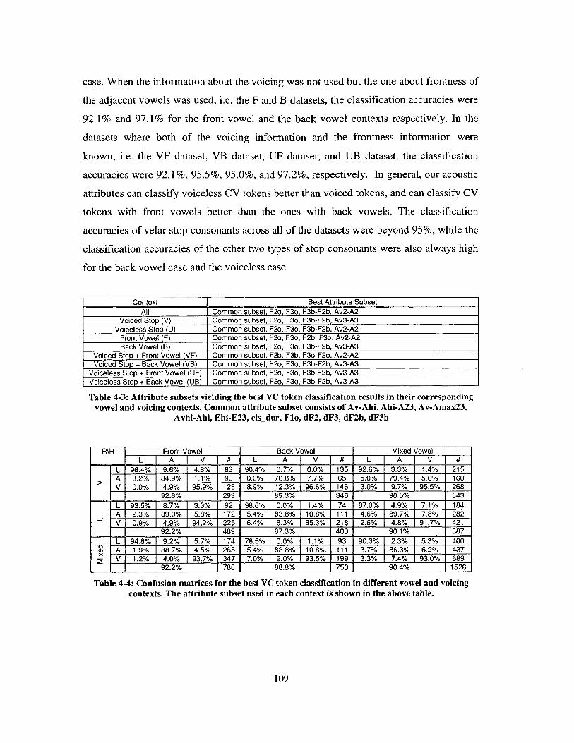
case. When the information about the voicing was not used but the one about frontness of
the adjacent vowels was used, i.e. the F and B datasets, the classification accuracies were
92.1% and 97.1% for the front vowel and the back vowel contexts respectively. In the
datasets where both of the voicing information and the frontness information were
known, i.e. the VF dataset, VB dataset, UF dataset, and UB dataset, the classification
accuracies were 92.1%, 95.5%, 95.0%, and 97.2%, respectively. In general, our acoustic
attributes can classify voiceless CV tokens better than voiced tokens, and can classify CV
tokens with front vowels better than the ones with back vowels. The classification
accuracies of velar stop consonants across all of the datasets were beyond 95%, while the
classification accuracies of the other two types of stop consonants were also always high
for the back vowel case and the voiceless case.
Context Best Attribute SubsetAll Common subset, F2o, F3o, F3b-F2b, Av2-A2
Voiced Stop (V) Common subset, F2o, F3o, F3b-F2b, Av3-A3Voiceless Stop (U) Common subset, F2o, F3o, F3b-F2b, Av2-A2
Front Vowel (F) Common subset, F2o, F3o, F2b, F3b, Av2-A2Back Vowel (B) Common subset, F2o, F3o, F3b-F2b, Av3-A3
Voiced Stop + Front Vowel (VF) Common subset, F2b, F3b, F3o-F2o, Av2-A2Voiced Stop + Back Vowel (VB) Common subset, F2o, F3o, F3b-F2b, Av3-A3
Voiceless Stop + Front Vowel (UF) Common subset, F2o, F3o, F3b-F2b, Av3-A3Voiceless Stop + Back Vowel (UB) Common subset, F2o, F3o, F3b-F2b, Av3-A3
Table 4-3: Attribute subsets yielding the best VC token classification results in their correspondingvowel and voicing contexts. Common attribute subset consists of Av-Ahi, Ahi-A23, Av-Amax23,
Avhi-Ahi, Ehi-E23, cls-dur, Flo, dF2, dF3, dF2b, dF3b
R\H Front Vowel Back Vowel Mixed VowelL A T V # L A | V # L A V #
L 96.4% 9.6% 4.8% 83 90.4% 0.7% 0.0% 135 92.6% 3.3% 1.4% 215A 3.2% 84.9% 1.1% 93 0.0% 70.8% 7.7% 65 5.0% 79.4% 5.6% 160V 0.0% 4.9% 95.9% 123 8.9% 12.3% 96.6% 146 3.0% 9.7% 95.5% 268
92.6% 299 89.3% 346 90.5% 643L 93.5% 8.7% 3.3% 92 98.6% 0.0% 1.4% 74 87.0% 4.9% 7.1% 184A 2.3% 89.0% 5.8% 172 5.4% I 83.8% 10.8% 111 4.6% 89.7% 7.8% 282V 0.9% 4.9% 94.2% 225 6.4% 8.3% 85.3% 218 2.6% 4.8% 91.7% 421
92.2% 489 87.3% 403 90.1% 887L 94.8% 9.2% 5.7% 174 78.5% 0.0% 1.1% 93 90.3% 2.3% 5.3% 400
1.9% 88.7% 4.5% 265 5.4% 83.8% 10.8% 111 3.7% 86.3% 6.2% 437V 1.2% 4.0% 93.7% ~347 7.0% 9.0% 93.5% 199 3.3% 7.4% 93.0% 689
92.2% 786 88.8% 750 90.4% 1526
Table 4-4: Confusion matrices for the best VC token classification in different vowel and voicingcontexts. The attribute subset used in each context is shown in the above table.
109

In the VC case, the classification accuracy when all of the stop consonants were mixed
together was 90.4%, which was 3.7% lower than the CV case. In this ALL dataset, as in
the CV case, velar stop consonants had the highest classification accuracy among the
three places of articulation. For the V and U datasets, the classification accuracies were
90.5% and 90.1% respectively. For the F and B datasets, the classification accuracies
were 92.2% and 88.8% respectively. And for the VF, VB, UF, and UB datasets, the
classification accuracies were 92.6%, 89.3%, 92.2%, and 87.3%. The dataset with the
highest classification accuracies for the VC case was the VF dataset. Unlike the CV case,
our acoustic attributes seemed to classify VC tokens with front vowels better than the
ones with back vowels. The classification accuracies were rather similar for the voiced
and voiceless case. In general, velar stop consonants were classified rather well in all of
the datasets, except for just the UB dataset, in which the classification accuracy of the
labial stop consonants was very high, i.e. 98.6% out of 74 labial stops.
4.3 LOOCV Classification Using Only Formant Information
As we can see in the last section, stop consonant places of articulation can be classified
quite well when we can obtain information from the release bursts as well as the formant
structures in the adjacent vowels. However, the presence of the release burst might be
absent. There are many cases where stop consonants are produced without the release
burst, especially in the VC tokens.
In this experiment, similar to the last experiment, LOOCV was used to evaluate the
classification accuracies in the 9 context-specific datasets. However, regardless of the
presence of the release burst, any tokens in each dataset that had all of the acoustic
attributes in the chosen acoustic attribute subset for each classification were included in
the classification. The acoustic attribute subset that yielded the best classification
accuracies for all contexts was {Flo, F2o, F3o, dF2, dF3} for both the CV and VC cases.
The confusion matrices are shown in Table 4-5 and Table 4-6 below.
110
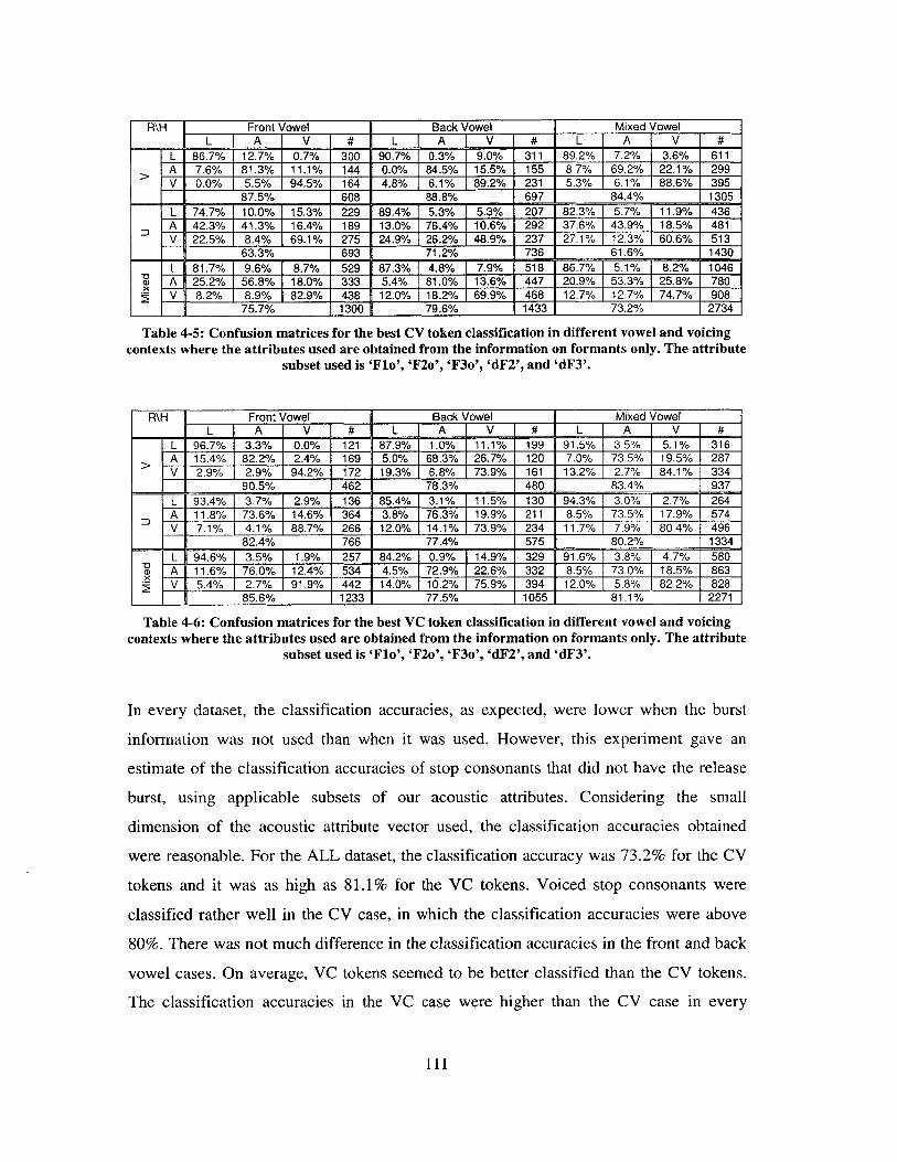
R\H Front Vowel Back Vowel Mixed VowelLI A J V # LI A V # L A V |#
L 86.7% 12.7% 0.7% 300 90.7% 0.3% 9.0% 311 89.2% 7.2% 3.6% 611>IA 7.6% 81.3% 11.1% 144 0.0% 84.5% 15.5% 155 8.7% 69.2% 22.1% 299
V 0.0% 5.5% 94.5% 164 4.8% 6.1% 89.2% 231 5.3% 6.1% 88.6% 39587.5% 608 88.8% 697 84.4% 1305
L 74.7% 10.0% 15.3% 229 89.4% 5.3% 5.3% 207 82.3% 5.7% 11.9% 436A 42.3% 41.3% 16.4% 189 13.0% 76.4% 10.6% 292 37.6% 43.9% 18.5% 481V 22.5% 8.4% 69.1% 275 24.9% 26.2% 48.9% 237 27.1% 12.3% 60.6% 513
63.3% 693 71.2% 736 61.6% 1430L 81.7% 9.6% 8.7% 529 87.3% 4.8% 7.9% 518 86.7% 5.1% 8.2% 1046A 25.2% 56.8% 18.0% 333 5.4% 81.0% 13.6% 447 20.9% 53.3% 25.8% 780T 8.2% 8.9% 82.9% 438 12.0% 18.2% 69.9% 468 12.7% 12.7% 74.7% 908
75.7% ;1300 1 79.6% 1433 , 73.2% ,2734
Table 4-5: Confusion matrices for the best CV token classification in different vowel and voicingcontexts where the attributes used are obtained from the information on formants only. The attribute
subset used is 'Flo', 'F2o', 'F3o', 'dF2', and 'dF3'.
R\H Front Vowel Back Vowel Mixed VowelL A V # L A V # L A V #
L 96.7% 3.3% 0.0% 121 87.9% 1.0% 11.1% 199 91.5% 3.5% 5.1% 316> A 15.4% 82.2% 2.4% 169 5.0% 68.3% 26.7% 120 7.0% 73.5% 19.5% 287
VA 2.9% 2.9% 94.2% 172 19.3% 6.8% 73.9% 161 13.2% 2.7% 84.1% 33490.5% 462 78.3% 480 83.4% 937
L= 34 3.7% 2.9% 136 185.4% 3.1% [11.5% 130 94.3% ]~3.0% 12.7%/ 264
D A 11.8% 73.6% 14.6% 364 j3.8% j76.3% 19.9% 211 J8.5% j73.5% j17.9% 574~V 7.1% 4.1% 88.7% 266 12.0% 14.1% 73.9% 234 11.7% 7.9% 80.4% 496
82.4% 766 77.4% 575 80.2% 11334L 94.6% 3.5% 1.9% 257 84.2% 0.9% 14.9% 329 91.6% 3.8% 4.7% 580A 11.6% 76.0% 12.4% 534 4.5% 72.9% 22.6% 332 8.5% 73.0% 18.5% 863
VJ 5.4% 2.7% 191.9% 442 14.0% .10.2% 75.9% -394 12.0%-. 5.8% 82.2%/ 82885.6% 1233 77.5% 1055 81.1% 2271
Table 4-6: Confusion matrices for the best VC token classification in different vowel and voicingcontexts where the attributes used are obtained from the information on formants only. The attribute
subset used is 'Flo', 'F2o', 'F3o', 'dF2', and 'dF3'.
In every dataset, the classification accuracies, as expected, were lower when the burst
information was not used than when it was used. However, this experiment gave an
estimate of the classification accuracies of stop consonants that did not have the release
burst, using applicable subsets of our acoustic attributes. Considering the small
dimension of the acoustic attribute vector used, the classification accuracies obtained
were reasonable. For the ALL dataset, the classification accuracy was 73.2% for the CV
tokens and it was as high as 81.1% for the VC tokens. Voiced stop consonants were
classified rather well in the CV case, in which the classification accuracies were above
80%. There was not much difference in the classification accuracies in the front and back
vowel cases. On average, VC tokens seemed to be better classified than the CV tokens.
The classification accuracies in the VC case were higher than the CV case in every
111

dataset. The front vowel case seemed to be better classified than the back vowel case,
regardless of the voicing, and voiced stops had a little higher classification accuracies
than the voiceless ones. Although the classification accuracies were lower due to the
absence of the release burst, our formant-related attributes were still performing well in
some datasets. Despite the small dimension of the acoustic attribute vector, the
classification accuracy was as high as 90.5% for the 462 stop consonants in the VC
dataset in the VC case.
4.4 Effect of Context Information
From the knowledge of the stop consonant production, we can conclude that the values of
some acoustic attributes distribute differently depending on the voicing of the stop and
the frontness of the adjacent vowel. The difference in the distributions of the values of the
attributes can be either dramatic or insignificant. If the former is the case, mixing
attribute values of the tokens with different contexts will increase the within-group
variability and result in a worse classification performance. In other words, if the value
distributions of some acoustic attributes depend dramatically on the contexts, taking those
contexts into account in doing the classification should improve the classification
accuracy. Specifically, if the classifier is trained on only the samples that belong to the
same context category as the test tokens, those test tokens should be better classified than
when the classifier is trained on tokens with mixed-context samples.
Note that the classification results in different contexts shown in section 4.2 and section
4.3 should not be compared to uncover the effect of context information since all of the
classification accuracies shown in those tables were obtained from different datasets, i.e.
the classification accuracies were evaluated on different sets of tokens. Therefore, not
only that the context information used is different but also that the classifications were
done on different sets of tokens contribute to the difference in the resulting classification
accuracies. Thus, we need to compare the classification results that were evaluated on the
same test tokens but the classifiers were trained on different fix-sized context-dependent
training sets.
112

Let the set of tokens with the context of interest be X and let its size be n. Also, let the set
of the rest of the tokens be Y and its size be m. Then, the tokens in X are the tokens for
which we would like to evaluate the classification accuracy. For the context-specific
training case, LOOCV is used on the set X to obtain the classification accuracy. For the
context-free training, we still want to evaluate the classification accuracy based on the
same set X. However, the cross validation method is different from LOOCV. In this case,
at the time when a token in X is to be classified, a training set is constructed by randomly
picking n-1 tokens from the combination of the set Y and the set X after the current test
token is left out. The classification accuracy is calculated by dividing the number of the
tokens in X that are correctly classified by n, the total number of tokens in X.
In order to be more confident about the classification accuracies resulting from randomly
picking the training tokens, the context-free classifications were done five times for each
test dataset. The average classification accuracy among the five iterations was calculated
and then compared with its context-specific counterpart. The results are shown in Table
4-7 to Table 4-10 below.
Test Sample Context Training Samples
Context Randomly PickedSpecific Average 1St 2 nd 3 rd 4 th 5th
Voiced (V) 92.8% 94.7% 95.1% 94.6% 94.7% 94.5% 94.5%Voiceless (U) 94.7 92.1% 92.2% 91.9% 92.5% 92.1% 91.6%
Front Vowel (F) 92.1% 90.3% 90.5% 90.4% 89.6% 90.9% 90.1%Back Vowel (B) 97.1% 95.9% 95.6% 95.9% 96.2% 95.8% 95.9%
Voiced+Front (VF) 92.1% 91.2% 90.9% 90.5% 91.5% 91.3% 91.8%Voiced+Back (VB) 95.5% 96.6% 96.6% 96.4% 96.6% 96.6% 96.6%
Voiceless+Front (UF) 95.2% 88.2% 88.6% 88.0% 87.8% 89.3% 87.5%Voiceless+Back (UB) 97.2% 93.9% 93.9% 94.5% 93.5% 93.6% 94.1%
Table 4-7: Classification accuracies in the context-specific training case and the context-free trainingcase for CV tokens across all voicing and frontness contexts.
Known Context % Classification Accuracies % Improvement P-value fromRandomly picked Context-specific McNemar'straining tokens training tokens significance test
Voicing 93.3% 93.8% 0.6% 0.52Frontness 93.3% 94.8% 1.6% 0.00
Voicing & Frontness 92.5% 95.2% 2.9% 0.00
Table 4-8: Comparison between the classification accuracies of CV tokens when some contexts areknown and when they are not known.
113

Table 4-7 shows that there was no large variation among the classification accuracies of
the same test dataset using the five randomly picked training sets. Thus the average
classification accuracies should represent the classification performances reasonably well
when the trainings were context-free. Comparing them with the classification accuracies
of the context-specific cases, we can see that most of the time classifiers that were trained
only on the tokens that had the same voicing and frontness contexts as the test tokens
gave better classification accuracies than the ones trained on the tokens with mixed
contexts. The only two datasets for which this was not the case are the V and VB
datasets.
However, Table 4-8 shows that when we knew either the voicing of the stop consonant,
the frontness of the adjacent vowel, or both, and used the right context-specific classifiers
to classify them, the classification accuracies were better. Also, we can see that knowing
the frontness of the adjacent vowel helped the place of articulation classification more
than knowing the voicing of the stop, and it was best to know both. The improvement
percentages were 0.6% when we knew only the voicing, 1.6% when we knew only the
frontness of the adjacent vowel and 2.9% when we knew the information on both of the
contexts. However, McNemar's statistical significance test showed that, with a
confidence level of 99%, the improvements in the classification accuracy were
statistically significant only when we knew the frontness and both the frontness and the
voicing. The P-values of the significance test are also shown in Table 4-8.
Test Sample Context Training Samples
Context Randomly PickedSpecific Average 1t 2 nd 3 rd 4th 5th
Voiced 90.5% 88.7% 88.0% 89.0% 88.3% 89.1% 89.3%Voiceless 89.9% 89.6% 89.6% 89.1% 89.8% 90.0% 89.5%
Front Vowel 91.8% 89.7% 89.8% 89.6% 89.8% 89.8% 89.5%Back Vowel 88.8% 88.3% 88.7% 88.8% 88.0% 87.8% 88.4%
Voiced+Front 92.3% 87.2% 86.8% 87.4% 87.7% 86.8% 87.4%Voiced+Back 89.3% 87.2% 87.9% 87.3% 86.1% 86.7% 88.2%
Voiceless+Front 91.9% 90.8% 91.0% 91.2% 90.2% 91.2% 90.6%Voiceless+Back 86.9% 85.8% 86.4% 85.6% 85.9% 85.4% 85.6%
Table 4-9: Classification accuracies in the context-specific training case and the context-free trainingcase for VC tokens across all voicing and frontness contexts.
114

Known Context % Classification Accuracies % Improvement P-value fromRandomly picked Context-specific McNemar'straining tokens training tokens significance test
Voicing 89.2% 90.2% 1.0% 0.18Frontness 89.0% 90.3% 1.5% 0.29
Voicing & Frontness 88.0% 90.1% 2.4% 0.02
Table 4-10: Comparison between the classification accuracies of VC tokens when some contexts areknown and when they are not known.
Similar to the CV case, Table 4-9 shows that there was also no large variation among the
classification accuracies of the same test dataset using the five randomly picked training
sets in the VC case. Thus the average classification accuracies of the VC tokens should
represent the classification performances when the trainings are context-free reasonably
well. Here, we can see classifiers that were trained only on the tokens that had the same
voicing and frontness contexts as the test tokens gave better classification accuracies than
the ones trained on the tokens with mixed contexts in every dataset.
Table 4-10 shows that when we know either the voicing of the stop consonant, the
frontness of the adjacent vowel, or both, and used the right context-specific classifiers to
classify them, the classification accuracies were better. The improvement percentages
were 1.0% when we knew only the voicing, 1.5% when we knew only the frontness of
the adjacent vowel and 2.4% if we knew the information on both of the contexts.
However, despite the improvements shown, the result of the statistical significance test,
with the confidence level of 99%, showed that none of them showed statistical
significance, unlike the CV case.
4.5 Classification of Stops that have Vowels on Both Sides
Up to this point, we implemented the place of articulation classification of CV and VC
tokens separately. Along with the information about the burst release, if applicable, we
made use of the information about the vowel on the right of the stop consonant in a CV
token, while the information of the vowel on the left was used for a VC token. However,
stop consonants in some of the CV and VC tokens were located between two vowels
(regardless of any word or syllable boundaries), and then there were CV and VC tokens
that shared these stop consonants. In predicting the place of articulation of these stop
115

consonants, it should intuitively be better to take the information on the vowels on both
sides of each stop consonant into account than to use only the information on the vowel
on either side of the stop consonant.
In this section, we will investigate the performances of different methods for combining
the information on the vowels on both sides of stop consonants in order to determine their
place of articulation. In this study, we proposed the combination of the information at two
levels: 1) the attribute-level combination, and 2) the classifier level combination.
In the attribute-level combination, one classification was performed for each of the stop
consonants that had a vowel on each side. The acoustic attribute that was used as the
classification feature vector of the classifier was constructed from the acoustic attributes
related to both of the vowels and the burst release of that stop, if these attributes existed.
This resulted in a classification feature vector that had more dimensions than the vectors
for the classification of its corresponding CV and VC tokens.
In the classifier-level combination, the information obtained from the vowels on both
sides of a stop consonant was not used together at first. The corresponding CV and VC
tokens were classified separately using their own set of acoustic attributes. However, the
decisions, from the CV and VC classifiers, about the place of articulation of the stop they
share were combined together in order to come up with only one final decision.
4.5.1 Attribute-level Combination
In this method of combining the related information on the vowel on both sides, we first
picked the acoustic attributes that would be used on each side as well as the acoustic
attributes that were presented in between, i.e. the burst-related acoustic attributes. These
acoustic attributes were picked based on the acoustic attribute subsets that gave the best
classification accuracies on the CV and VC tokens in the ALL dataset, as shown in
section 4.2 and section 4.3. If the selection of acoustic attributes related to the burst of the
CV and VC cases did not agree, the acoustic attributes used in the CV case were picked.
116
With burst release, the selected acoustic attributes related to the vowels on the right side
of the stops were VOT, Flo, dF2, dF3, dF2b, dF3b, F2b, F3b, and F3o-F2o. The acoustic
attributes related to the vowels on the left were CLSDUR, Flo, dF2, dF3, dF2b, dF3b,
F2o, F3o, and F3b-F2b. The acoustic attributes related to the release burst were Av3-A3,
Av-Ahi, Ahi-A23, Av-Amax23, Avhi-Ahi, Ehi-E23, and cgF20a. The three sets of
acoustic attributes were concatenated. Therefore, this resulted in an acoustic attribute
vector whose dimension was 25.
Without using the burst information, the selected acoustic attributes related to the vowels
on the right side of the stops were Flo, F2o, F3o, dF2 and dF3. The same set of acoustic
attributes was used for the information on the left side. The dimension of the resulting
acoustic attribute vector in this case was 10.
Table 4-11 to Table 4-14 show the confusion matrices when stop consonants that had
vowels on both sides were classified based on their CV and VC tokens respectively. The
classifications here did not make use of the voicing and the frontness contexts. The
acoustic attributes used for the CV token classifications included the acoustic attributes
related to the vowel on the right side and the acoustic attributes that described the release
burst, if applicable, while the ones used for the VC token classification included the
acoustic attributes related to the vowel on the left side and the ones describing the release
burst, if applicable.
Table 4-11 and Table 4-13 show the confusion matrices of the place of articulation
classifications of the CV tokens whose stop consonants also had their adjacent vowels on
the left, i.e. there were VC tokens that shared these stop consonants. The classification in
the former one made use of the acoustic attributes that required the presence of the
release bursts, while the latter one used only the information on the formant structures.
Table 4-12 and Table 4-14 show the confusion matrices of the place of articulation
classifications of the VC tokens whose stop consonants also had their adjacent vowels on
the right. Again, the classification in the former one made used of the acoustic attributes
that required the presence of the release bursts, while the latter one used only the
117
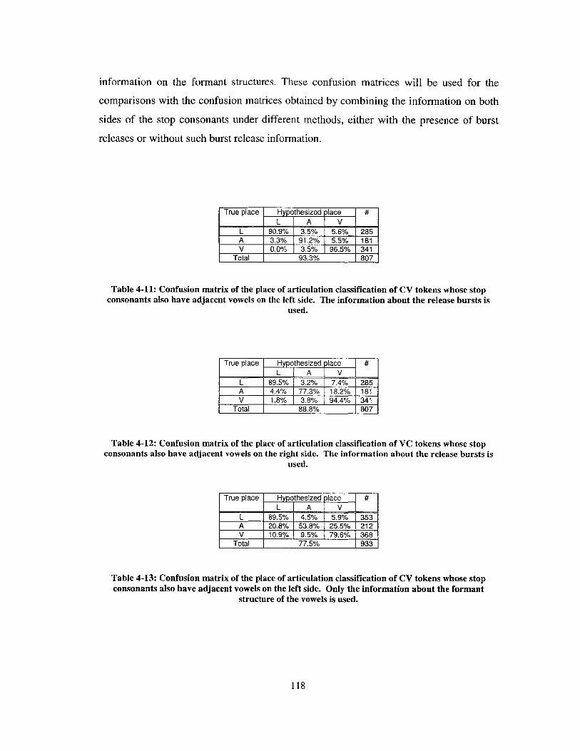
information on the formant structures. These confusion matrices will be used for the
comparisons with the confusion matrices obtained by combining the information on both
sides of the stop consonants under different methods, either with the presence of burst
releases or without such burst release information.
True place Hypothesized )lace #L A V
L 90.9% 3.5% 5.6% 285A 3.3% 91.2% 5.5% 181V 0.0% 3.5% 96.5% 341
Total 93.3% 807
Table 4-11: Confusion matrix of the place of articulation classification of CV tokens whose stopconsonants also have adjacent vowels on the left side. The information about the release bursts is
used.
FTrue place Hyp othesized >lace #
L A VL 89.5% 3.2% 7.4% 285A 4.4% 77.3% 18.2% 181V 1.8% 3.8% 94.4% 341
Total 88.8% 807
Table 4-12: Confusion matrix of the place of articulation classification of VC tokens whose stopconsonants also have adjacent vowels on the right side. The information about the release bursts is
used.
True place Hypothesized lace #L A V
L 89.5% 4.5% 5.9% 353A 20.8% 53.8% 25.5% 212V 10.9% 9.5% 1 79.6% 368
Total 77.5% 933
Table 4-13: Confusion matrix of the place of articulation classification of CV tokens whose stopconsonants also have adjacent vowels on the left side. Only the information about the formant
structure of the vowels is used.
118

True place Hyp othesized lace #L A V
L 90.7% 4.0% 5.4% 353A 8.0% 68.9% 23.1% 212V 13.0% 4.6% 82.3% 368
Total 82.4% 933
Table 4-14: Confusion matrix of the place of articulation classification of VC tokens whose stopconsonants also have adjacent vowels on the right side. Only the information about the formant
structure of the vowels is used.
Table 4-15 and Table 4-16 show the confusion matrices when the place of articulation
classifications were done by combining the acoustic attributes on both sides of the stops
together. In the former table, only the tokens whose stops contained release bursts were
considered, while in the latter table, the information on the release bursts were not used.
Thus, the tokens included in the dataset did not have to contain the release bursts.
The classifications here did not use the information on the voicing of the stops and the
frontness of the vowels. Table 4-15 shows, for the case with release bursts, that among all
of the 807 stops with release bursts that had vowels on both sides, the overall
classification accuracy was 94.3%, which was 1.1% and 6.2% better than the cases where
the place of articulation decisions were made from the information on CV tokens and VC
tokens alone respectively. 94.7% of 285 labial stop consonants were correctly classified
with the information on both sides. This was, respectively, 4.2% and 5.8% better than the
labial classification accuracies based on the CV and VC information alone. For the 181
alveolar stop consonants, the classification accuracy was 87.3%, which was, however,
4.3% worse than the classification accuracies based on the CV information alone. Still, it
was 12.9% better than the classification accuracies based on the VC information alone.
The classification accuracy of alveolar stops using the VC information alone was much
lower than when the CV information was used. And, when the two sources of
information were combined, the VC information somehow confused the classifier.
Instead of complimenting each other, the combined information led to the lower
classification accuracy than when the CV information was used alone. For the 341 velar
stop consonants, the classification accuracy based on the combined information was
97.7%, which was, respectively, 1.2% and 3.5% better than its CV and VC counterparts.
119
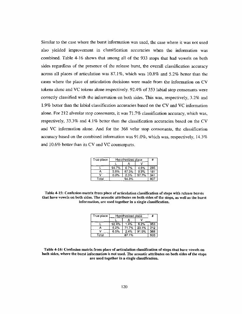
Similar to the case where the burst information was used, the case where it was not used
also yielded improvement in classification accuracies when the information was
combined. Table 4-16 shows that among all of the 933 stops that had vowels on both
sides regardless of the presence of the release burst, the overall classification accuracy
across all places of articulation was 87.1%, which was 10.8% and 5.2% better than the
cases where the place of articulation decisions were made from the information on CV
tokens alone and VC tokens alone respectively. 92.4% of 353 labial stop consonants were
correctly classified with the information on both sides. This was, respectively, 3.2% and
1.9% better than the labial classification accuracies based on the CV and VC information
alone. For 212 alveolar stop consonants, it was 71.7% classification accuracy, which was,
respectively, 33.3% and 4.1% better than the classification accuracies based on the CV
and VC information alone. And for the 368 velar stop consonants, the classification
accuracy based on the combined information was 91.0%, which was, respectively, 14.3%
and 10.6% better than its CV and VC counterparts.
True place Hyp othesized >lace #L A V
L 94.7% 0.7% 4.6% 285A 2.8% 87.3% 9.9% 181V 0.0% 2.3% 97.7% 341
Total 94.3% 807
Table 4-15: Confusion matrix from place of articulation classification of stops with release burststhat have vowels on both sides. The acoustic attributes on both sides of the stops, as well as the burst
information, are used together in a single classification.
True place Hyothesized Alace #L A V
L 92.4% 1.4% 6.2% 353A 5.2% 71.7% 23.1% 212V 6.5% 2.4% 1 91.0% 368
Total 87.1% 933
Table 4-16: Confusion matrix from place of articulation classification of stops that have vowels onboth sides, where the burst information is not used. The acoustic attributes on both sides of the stops
are used together in a single classification.
120

The consistent improvements shown in every case indicate that, in classifying the place
of articulation of a stop consonant, the information on the vowels on both sides of that
stop should be gathered and used, along with the information on its release burst,
whenever this is available.
Next, we will investigate the performance of another way to combine the information on
both sides of a stop consonant.
4.5.2 Classifier-level Combination
Here, instead of combining the acoustic attributes from both sides of the stop consonants
into longer acoustic attribute vectors and performing one classification for each stop
consonant, we used two classifiers for each stop consonant. One of them was responsible
for classifying the place of articulation of that stop based on its corresponding CV token
while the other one used the information in the stop's corresponding VC tokens. Each
classifier made the decision about the place of articulation of that stop consonant
separately based on its corresponding set of acoustic attributes. Then, the posterior
probabilities for each place of articulation of that stop proposed from the two classifiers
were combined and the most likely place of articulation resulting from the combination
of the probabilities was chosen as the final decision for that stop consonant. The acoustic
attributes used for the CV and VC token classifiers were the acoustic attributes that gave
the best classification performance in the corresponding experiments in this chapter.
These choices of acoustic attributes were similar to the ones in the attribute-level
combination case.
We proposed two ways of combining the posterior probabilities from the CV and VC
classifiers. The first one was called the sum rule and the other one was called the product
rule.
121

The combined posterior probability, P(Placei I X), from the sum rule was obtained from:
_ N N
P(Place I X) =Ly'Pj (Place, I X) ; r =1 Eq.4-2j=1 j=1
where:
- P(Place, I Xj) is the probability that the place of articulation of the stop consonant is
labial (i=1), alveolar (i=2), or velar (i=3), based on the observation X j, the acoustic
attributes used by thej jh classifier. (j=1,...,N)
- rj is the weight of the probability obtained from the j classifier.
- N is the number of the classifiers used.
The combined posterior probability, P(Place I X), from the product rule was obtained
from:
N__
11 P (Place, I X j)
P(Place, I X) -N Eq.4-3
YHPj,(Place \ X)" 'k=1 j=1
where:
- P(Place I X1 ) is the probability that the place of articulation of the stop consonant is
labial (i= 1), alveolar (i=2), or velar (i=3), based on the observation Xj, the acoustic
attributes used by the/ jh classifier. (j=1,...,N)
- y is the weight of the probability obtained from the jth classifier.
- N is the number of the classifiers used.
In both combination rules, we had the flexibility to weigh the decision made by the N
classifiers differently. In this case, N is equal to two. The first classifier proposed how
likely that the place of articulation of a given stop consonant was labial, alveolar, or velar
122

by using the information from the CV token formed by that stop, and the other classifier
did so by using the information from the VC token formed by that stop. By adjusting the
weights for the probabilities of each place of articulation from the two classifiers, we
adjusted the level of confidence in the classification performances of the two classifiers.
In the sum rule, the two weights must sum to one for the resulting posterior probability to
be valid. Also, the same weight restriction was applied to the product rule, although it
was not necessary.
Figure 4-2 shows the classification accuracies when the places of articulation of stop
consonants with release bursts were classified using the classifier-level combination
under the sum rule and the product rule. The weight given to the posterior probability
obtained from the VC classifier was varied from 0 to 1. When the weight for the VC
classifier was 0 and the weight for the CV classifier was 1, or vice versa, we used the
decision from only one of the two classifiers. Thus, the classification accuracies at these
weights were the same as the ones obtained by using one of the classifiers only. Under
both rules, the classification accuracies were greater when both classifiers contribute to
the combined decision. The classification accuracies under both rules seemed to be
maximized when the importance of both classifiers was rather equal or, in other words,
the difference between the two weights was not extreme. Under the sum rule, the
classification accuracy was maximized when equal weights were given to the two
classifiers. Under the product rule, the optimal weights were 0.400 for the VC classifier
and 0.600 for the CV classifier. The maximum classification accuracies under the sum
and the product rules were 94.9% and 95.5% respectively. Their respective corresponding
confusion matrices are shown in Table 4-19 and Table 4-20. In order to explore the
improvement in classification accuracy when the information in both CV and VC tokens
were combined, the confusion matrices obtained from classifying the same set of stop
consonants by using the CV token classifier and the VC token classifier separately are
shown in Table 4-17 and Table 4-18.
123

90f
0 0.1 0.2 0.3 0.4 0.5 0.6VC weight
Figure 4-2: Classification accuracy percentage of the place of articulation of stop consonants withrelease bursts using the combined classifiers under the product rule and the sum rule, when the
weight used for the posterior probability obtained from the VC classifier varies from 0 to 1
True place Hyphesized lace #L A V
L 89.5% 3.8% 6.6% 286A 3.4% 90.4% 6.2% 178V 0.3% 3.3% 96.4% 336
Total 92.6% 800
Table 4-17: Confusion matrix of the place of articulation classification of the same set of stopconsonants used in the classifier-level combination experiment based on the information from the CV
tokens. The information about the release bursts is used.
True place Hypothesized >lace #L A V
L 90.2% 3.5% 6.3% 286A 3.4% 80.9% 15.7% 178V 3.6% 6.3% 90.2% 336
Total 88.1% 800
Table 4-18: Confusion matrix of the place of articulation classification of the same set of stopconsonants used in the classifier-level combination experiment based on the information from the VC
tokens. The information about the release bursts is used.
124
93
S92
91
Product- Sum
89
0.7 0.8 0.9
LIK
.
95
94
I

True place Hyp othesized lace #L A V
L 94.8% 1.0% 4.2% 286A 4.5% 89.3% 6.2% 178V 0.9% 1.2% , 97.9% 336
Total 94.9% 800
Table 4-19: Confusion matrix of the place of articulation classification using the classifier-levelcombination under the sum rule with the VC weight equals to 0.5 and the CV weight equals to 0.5.
The information about the release bursts is used.
True place Hyp othesized lace #L A V
L 94.8% 1.0% 4.2% 286A 2.8% 92.1% 5.1% 178V 0.6% 1.5% 1 97.9% 336
Total 95.5% 800
Table 4-20: Confusion matrix of the place of articulation classification using the classifier-levelcombination under the product rule with the VC weight equals to 0.4 and the CV weight equals to
0.6. The information about the release bursts is used.
Table 4-19 and Table 4-20 suggest that the combination using the product rule achieved
the higher maximum accuracy than using the sum rule. However, under any choice of
weights used, except zero weights, both combination rules produced higher classification
accuracies than the classification that used only either the CV or VC information. The
maximum classification accuracy of the combination under the sum rule was 94.9%,
which was 2.5% and 7.7% higher than its CV and VC counterparts respectively. Among
the 286 labial stop consonants, 94.8% were classified correctly. This percentage was
5.9% higher than its CV counterpart and 5.1% higher than its VC counterpart. Among the
178 alveolar stop consonants, 89.3% were classified correctly. This was 1.2% worse than
the classification accuracy of the CV token classifier. However, it was 10.4% higher than
the one obtained from the VC token classifier. The degradation from the CV case in the
alveolar classification accuracy is similar to what was found in the attribute-level
combination, and it can be explained in the same fashion ( i.e. due to the fact that the VC
classifier gave a much lower alveolar classification accuracy than its CV counterpart).
97.9% of 336 velar stop consonants were classified correctly. This was 1.6% and 8.5%
better than its CV and VC counterparts.
125

Under the better rule, which is the product rule, the maximum classification accuracy was
95.5%, which was 3.1% and 8.4% higher than its CV and VC counterparts respectively.
Among the 286 labial stop consonants, 94.8% were classified correctly. This percentage
was 5.9% higher than its CV counterpart and 5.1% higher than its VC counterpart.
Among the 178 alveolar stop consonants, 92.1% were classified correctly. This
percentage was 1.9% and 13.8% higher than its CV and VC counterparts respectively. It
is worth noting that, under this combination method, the combined information led to a
better classification accuracy than either one of the CV and VC classifiers, even though
the classification accuracy of the VC classifier was much lower than its CV counterpart.
97.9% of 336 alveolar stop consonants were classified correctly. This was 1.6% and 8.5%
better than its CV and VC counterparts.
Figure 4-3 shows the classification accuracies when the place of articulation of stop
consonants were classified using the classifier-level combination under the sum rule and
the product rule regardless of the presence of the release bursts. In the fashion similar to
Figure 4-2, the weight given to the posterior probability obtained from the VC classifier
was varied from 0 to 1. Under both rules, the classification accuracies were greater when
both classifiers contribute to the combined decision. The classification accuracies under
both rules seemed to be maximized when the difference between the two weights was not
too extreme. Under the sum rule, the optimal weights were 0.475 for the VC classifier
and 0.525 for the CV classifier. Under the product rule, the optimal weights were 0.375
for the VC classifier and 0.625 for the CV classifier. The maximum classification
accuracies under the sum and the product rules were 86.7% and 87.5% respectively.
Their corresponding confusion matrices are shown in Table 4-23 and Table 4-24
respectively. The confusion matrices obtained from classifying the same set of stop
consonants by using the CV token classifier and the VC token classifier separately are
shown in Table 4-21 and Table 4-22.
126

0.1 0.2 0.3 0.4 0.5VC weight
0.6 0.7 0.8 0.9
Figure 4-3: Classification accuracy percentage of the place of articulation of stop consonants usingthe combined classifiers under the product rule and the sum rule, when the weight used for theposterior probability obtained from the VC classifier varies from 0 to 1. The information about
release bursts is not used.
True place Hyp othesized lace #L A V
L 89.5% 4.5% 6.0% 352A 20.8% 53.8% 25.5% 212V 10.9% 9.6% 79.5% 366
Total 77.4% 930
Table 4-21: Confusion matrix of the place of articulation classification of the same set of stopconsonants used in the classifier-level combination experiment based on the information from the CV
tokens. The information about the release bursts is not used.
True place Hyp othesized )lace #L A V
L 89.8% 4.5% 5.7% 352A 5.2% 73.6% 21.2% 212V 12.8% 6.3% 80.9% 366
Total 82.6% 930
Table 4-22: Confusion matrix of the place of articulation classification of the same set of stopconsonants used in the classifier-level combination experiment based on the information from the VC
tokens. The information about the release bursts is not used.
127
A
861
84
82Ma
78
76 L0
Product--- Sum
I
80

True place Hyp othesized >lace #L A V
L 94.6% 1.1% 4.3% 352A 9.0% 70.3% 20.8% 212V 9.6% 1.9% 88.5% 366
Total 86.7% 930
Table 4-23: Confusion matrix of the place of articulation classification using the classifier-levelcombination under the sum rule with the VC weight equals to 0.475 and the CV weight equals to
0.525. The information about the release bursts is not used.
True place Hypothesized >lace #L A V
L 94.6% 1.1% 4.3% 352A 9.0% 71.7% 19.3% 212V 8.2% 1.9% 89.9% 366
Total 87.5% 930
Table 4-24: Confusion matrix of the place of articulation classification using the classifier-levelcombination under the product rule with the VC weight equals to 0.375 and the CV weight equals to
0.625. The information about the release bursts is not used.
Similar to the results obtained in the stop consonants with release burst case, Table 4-23
and Table 4-24 show that the combination using the product rule achieved the higher
maximum accuracy than using the sum rule. Also, under any choices of weights used,
except zero weights, both combination rules produced higher classification accuracies
than the classification that used only either the CV or VC information. The maximum
classification accuracy of the combination under the sum rule was 86.7%, which was
11.9% and 4.9% higher than its CV and VC counterparts respectively. Among the 352
labial stop consonants, 94.6% were classified correctly. This percentage was 5.7% higher
than its CV counterpart and 5.3% higher than its VC counterpart. Among the 212 alveolar
stop consonants, 70.3% were classified correctly. This was 30.7% better than the
classification accuracy of the CV token classifier. However, it was 4.5% worse than the
one obtained from the VC token classifier. Again, this degradation can be explained by
the fact that the classification accuracy obtained from the CV information is much lower
than the one obtained from the VC information. 88.5% of 366 velar stop consonants were
classified correctly. This was 11.3% and 9.4% better than its CV and VC counterparts.
128

Under the product rule, the maximum classification accuracy was 87.5%, which was
13.0% and 6.0% higher than its CV and VC counterparts respectively. Among the 352
labial stop consonants, 94.6% were classified correctly. This percentage was 5.7% higher
than its CV counterpart and 5.3% higher than its VC counterpart. Among the 212 alveolar
stop consonants, 71.7% were classified correctly. This was 33.3% better than the
classification accuracy of the CV token classifier. However, it was 2.6% worse than the
one obtained from the VC token classifier. The degradation can be explained similarly to
what happened in the sum rule. 89.9% of 366 alveolar stop consonants were classified
correctly. This was 13.1% and 6.0% better than its CV and VC counterparts.
Note that there were some slight differences in the set of tokens used in the attribute-level
combination experiment and the classifier-level combination experiment. These
differences were due to the removal of the outliers. In the attribute-level combination
experiment, outliers were identified based on the values of only the tokens that had
vowels on both sides and had all of the acoustic attributes chosen to be used for the
corresponding classifications. However, in the classification-level combination
experiment, since, in the first stage, classifiers were used on the CV and VC tokens
separately, outliers were then identified based on the values of all of the CV or VC tokens
that had all of the required acoustic attributes, regardless of the presence of their CV or
VC token counterparts. Despite the differences, the majority of the tokens were the same.
In both the case in which the burst information was used and the case in which it was not,
the differences between the tokens in the attribute-level combination experiment and the
classifier-level combination experiment were less than 1% of the total number of the
tokens in both experiments. Thus, roughly, it was reasonable to compare the
classification results obtained under the two combination strategies, if the classification
accuracies from the two experiments were different more than 1%.
Table 4-25 summarizes the classification accuracy percentages of the VC classifier, the
CV classifier, the attribute-level combination classification, and the classifier-level
combination classification under the sum rule and the product rule. As mentioned, the
classification accuracies were higher whenever the information on both sides of the stop
129

consonants was used. The combining method that yielded the highest classification
accuracy for the dataset used here was the classifier-level combination under the product
rule regardless of the presence of the release burst. McNemar's statistical significance
test showed that the improvement gained in the classification accuracy by using the
combined information using either level of the two combinations was statistically
significant with a confidence level of 99%. However, the classification accuracies
obtained from different methods of combining were not significantly different with the
same confidence level.
Classifier % Accuracy using burst info. % Accuracy not using burst info.VC -88% -82%CV -93% -77%
Attribute-level 94.3% 87.1%Sum Rule 94.9% 86.7%
Product Rule 95.5% 87.5%
Table 4-25: % Classification accuracy comparison among different classification approaches
4.6 Evaluation on the SP Database
At this point, we wished to evaluate our classification scheme on all of the qualified
tokens in the SP database. Note that the tokens used in each of the classification
experiments reported earlier in this chapter were a subset of all of the tokens in the SP
database, which had the contexts of interest for their associated experiments. Also, the
tokens used for the calculation of the classification accuracies in different experiments
were not mutually exclusive. Consequently, the overall classification accuracy based on
all of the tokens in the SP database cannot be calculated from the classification results of
those experiments. Here, each of the tokens in the SP database was classified by using the
method tailored to its contexts. Specifically, tokens were classified by the classifiers that
were trained on the test tokens that had similar contexts. The contexts that were taken
into account included the frontness of the adjacent vowels, the voicing of the stop
consonants, the presence of the release bursts, and the location of the adjacent vowels, i.e.
VC, CV, or VCV. The decision about the place of each stop consonant was made
according to the process shown in the diagram in Figure 4-4.
130

Qualified stop consonant
Yes context isa vowel ?
Classificationbased on VC <-------------------- --------------- Voicing and frontness
tokens t context
a vowe ?
ClassificationVoicing and frontness -------------------------------- based on CV
context No tokens
vCVYes No
Combine Final decisionclassification classification resultresu s fr from either VC or
tokens
Final decision =
combinedclassification result
IFinal decision
Figure 4-4: Place of articulation classification process for the qualified tokens in the SP database
131

For each stop consonant, if the segment located immediately to its left was a vowel, i.e.
that stop consonant belonged to a VC token, it was classified based on the sample dataset
constructed from other VC tokens with the same voicing and frontness contexts. If that
stop consonant contained a release burst, the information of that release burst was used.
Only the VC tokens whose stop consonants contained release bursts were included in the
training set, and the acoustic attributes used were the ones listed in Table 4-3. If there was
no release burst, the acoustic attributes used were Flo, F2o, F3o, dF2, and dF3, and the
training data of these acoustic attributes were obtained from all of the VC tokens with
similar voicing and frontness contexts, regardless of the presence of the release burst. The
hypothesized place of articulation and the posterior probabilities of the three places of
articulation were then stored.
If the segment located immediately to the right of a stop consonant was a vowel, i.e. that
stop consonant belonged to a CV token, the process similar to the VC case was conducted
with the training set constructed from CV tokens instead. The information about the
voicing of the stop consonant, the presence of the release burst, and the frontness of the
adjacent vowel was used in the same way as the VC case. Under the presence of the
release burst, the acoustic attributes in Table 4-1 were used; otherwise Flo, F2o, F3o,
dF2, and dF3 were used. Then, the decision about the place of articulation along with the
posterior probabilities of the three places of articulation from the CV classifier were
stored.
If both the CV and VC tokens corresponding to the current stop consonant existed, the
decisions made by the CV and VC classifiers were combined. The final posterior
probabilities for the three places of articulation were calculated using the product rule,
mentioned in the earlier section. In the case where the release burst information was used
in the CV and VC classifier, the weights given to the posterior probabilities from the VC
classifier and the CV classifier were 0.400 and 0.600, respectively. They were 0.375 and
0.625 for the case when the burst release did not exist. The final hypothesis about the
place of articulation was the one that has the maximum posterior probability resulting
from the combination of the two classifiers. However, if the stop consonant did not have
132

vowels on both side of it, the final hypothesis about the place of articulation was the
place hypothesized by either the CV or VC classifier, whichever applied.
The classification result obtained from the process described above can be broken down
to confusion matrices shown in Table 4-26 to Table 4-29. The matrices show the
classification results on stop consonants with vowels on both sides, stop consonants with
vowels only to the left, stop consonants with vowels only to the right, and the overall
classification result. The stop consonants with and without burst were also separated. The
classification accuracy in each confusion matrix was calculated by dividing the number
of correctly classified stop consonants that belonged to that matrix by the total number of
stop consonant that belonged to that matrix. Note that the stop consonants that were parts
of the same confusion matrix were not necessary classified based on the same training
set.
VCV with burst
Hypothesized placeL A V
95.8% 1.4% 2.8%1.1% 94.4% 4.5%0.9% 0.6% 98.5%
285178336
Total 1 96.6% [799](a)
True place Hypohesized >lace #L A V
L 96.5% 1.2% 2.3% 345A 3.4% 91.2% 5.4% 205V 1.1% 0.6% 98.3% 353
Total 96.0% 903
True place
LAV
Total
VCV with no burst
Hypothesized placeL A V
100.0% 0.0% 0.0%18.5% 70.4% 11.1%5.9% 0.0% 94.1%
91.3%(b)
#602717
104
All VCV
(c)
Table 4-26: Confusion matrices from the place of articulation classification of the stop consonants inthe SP database that have vowels on both sides. The stop consonants in (a) contain the release burst,
while in (b) they do not. The confusion matrix in (c) is the combination of the results from (a) and (b).
133
True place
LAV
i

CV with burst
True place Hyp othesized place #L A Vi
L 92.3% 3.0% 4.6% 624A 1.5% 96.0% 2.6% 548V 0.8% 1.9% 97.3% 528
Total 95.1% 1700(a)
True place ___HyJp othesized >lace_ #L A V
L 92.1% 3.2% 4.7% 683A 1.8% 95.6% 2.7% 563V 0.8% 2.1% 97.2% 529
Total 94.7% 1775
CV with no burst
True place H othesized lace #L A V
L 89.8% 5.1% 5.1% 59A 13.3% 80.0% 6.7% 15V 0.0% 100.0% 0.0% 1
Total 86.7% 75(b)
All CV
(c)
Table 4-27: Confusion matrices from the place of articulation classification of the stop consonants inthe SP database that have vowels on their right sides only. The stop consonants in (a) contain the
release burst, while in (b) they do not. The confusion matrix in (c) is the combination of the resultsfrom (a) and (b).
VC with burst VC with no burst
True place Hyp othesized >lace #*L A V
L 87.6% 3.5% 8.8% 113A 4.3% 85.3% 10.5% 258V 1.1% 2.9% 96.0% 349
Total 90.8% 720(a)
True place Hypothesized place #L A IV
L 88.0% 3.6% 8.4% / 25~A 8.7% 78.6% 12.7% 646V 2.2% 2.6% 95.2% 458
Total 85.9% J32
True place Hyp othesized lace #*I L A V
L 88.4% 3.6% 8.0% 112A 11.6% 74.2% 14.2% 388V 5.5% 1.8% 92.7% 109
Total 80.1% 609(b)
All VC
(c)
Table 4-28: Confusion matrices from the place of articulation classification of the stop consonants inthe SP database that have vowels on their left sides only. The stop consonants in (a) contain the
release burst, while in (b) they do not. The confusion matrix in (c) is the combination of the resultsfrom (a) and (b).
134

Stop consonants with burst Stop consonant with no burst
True place Hypothesized place # True place Hypothesized lace #
SL [A V I L A VL 92.8% 2.6% 4.6% 1022 L 91.8% 3.0% 5.2% 231A 2.1% 92.9% 5.0% 984 A 12.1% 74.2% 13.7% 430V 0.9% 1.8% 97.3% 1213 V 5.5% 2.4% 92.1% 127
Total 94.5% 3219 Total 82.2% 788(a) (b)
All stop consonant
True place Hypothesized >lace #L A V
L 92.6% 2.7% 4.7% 1253A 5.2% 87.2% 7.6% 1414V 1.3% 1.9% 96.8% 1340
Total 92.1% 4007(c)
Table 4-29: Confusion matrices from the place of articulation classification of the stop consonants inthe SP database. The stop consonants in (a) contain the release burst, while in (b) they do not. The
confusion matrix in (c) is the combination of the results from (a) and (b).
The overall classification accuracy of the 4007 stop consonants was 92.1 %. The largest
portion of the error came from alveolar stops. Among the three types of stop consonants,
alveolar stop consonants were the ones that are misclassified the most. 12.8% of the 1414
alveolar stop consonants were incorrectly classified, while they were 7.4% and 3.2% for
the 1253 labial and 1340 velar stop consonants. The classification accuracies were always
lower for the stop consonants that did not contain the release bursts than the ones that had
them. This is reasonable since the former case had a smaller amount of information to be
used in classification. The dimensions of the acoustic attribute vectors used in the
classifications were much smaller when there were no release bursts. The classification
accuracies were quite high when stop consonants were adjacent to vowels on both sides,
even in the case where the release bursts did not exist. The overall classification accuracy
for this group of stop consonants was 96.0%, regardless of the release bursts. It was
96.6% when the bursts existed and 91.3% when they were not. The classification of stop
consonants that had vowels only to the right (CV) seemed to do better than the
classification of stop consonants that had vowels only to the left (VC). The corresponding
classification accuracies were 94.7% and 85.9% for the CV and VC cases respectively.
135

VCV with burst
VCV without burst2.8% VC without burst
8.6%
38.2%CV with burst 26.3%
20.9%
3.2%
CV without burst
VC with burst
Figure 4-5: Distribution of the classification error
The 4007 stop consonants classified here can be categorized into the following 6 non-
overlapping groups: VCV with burst, VCV without burst, CV with burst, CV without
burst, VC with burst, and VC without burst. The distribution of the classification errors is
shown in Figure 4-5. The biggest slice in the chart was from the VC without burst group,
which was responsible for 38.2% of the total classification error. From the confusion
matrices, we can see that this group also yielded the lowest classification accuracy
percentage among the 6 groups; the number of the stop consonants belonging to this
group was 609, or 15.2% of the total number of stop consonants classified here. The next
two biggest slices were from the CV with burst and VC with burst groups. However,
these groups had rather high classification accuracy percentages. This indicates that one
possibility in improving the classification accuracy is to try to reduce the classification
error of VC tokens with no burst.
The top pane of Figure 4-6 shows the number of the correctly classified stops in the
probability ranges according to their posterior probabilities of the hypothesized places.
The bottom pane shows the number of the incorrectly classified stops in the same
posterior probability ranges. From the top histogram, we can see that the majority of the
136

correctly classified places of articulation had high posterior probabilities, which was
encouraging. More than 90% of the correctly classified places of articulation had the
posterior probabilities of more than 0.8. However, the bottom histogram suggests that
there were also many stop consonants whose places of articulation were incorrectly
classified that have the posterior probabilities of more than 0.8. Still, the number of such
stop consonants was far less than in the correctly classified case.
Figure 4-7 shows the relationship between the percentages of stop consonants whose
places of articulation are correctly classified in various posterior probability ranges and
the corresponding posterior probability range. This plot was constructed from the
numbers of correctly and incorrectly classified stop consonants in the histograms in
Figure 4-6. Approximately, the plot is close to a straight line with a slope of 1.0,
suggesting that if a stop consonant is classified to a particular place of articulation, the
probability that the hypothesized place of articulation is the true place of articulation is
similar to the posterior probability of that hypothesized place of articulation, especially
when the posterior probability of that place of articulation is higher than 0.7. However,
for the posterior probability of less than 0.7, the probability that the hypothesized place of
articulation is the same as the true place of articulation might be a little higher than the
posterior probability. Nevertheless, we should be able to conclude that the posterior
probability obtained by our classification process in this section is a reasonable measure
of the probability of the true place of articulation.
137

Histogram of correctly classified tokens150
126 149 3216
102100-
80
1750
0.4 0.5 0.6 0.7 0.8 0.9 1Posterior probability
Histogram of incorrectly classified tokens140
120- 122
100-
80-
60- 53 5040 40 35
20- 17
0.4 0.5 0.6 0.7Posterior probability
0.8 0.9 1
Figure 4-6: Histogram of the posterior probabilities corresponding to the hypothesized place ofarticulation. The top histogram shows the number of the correctly classified stop consonants in
different probability ranges. The bottom histogram shows the number of the incorrectly classifiedstop consonants in different probability ranges.
below 0.5 0.5-0.8 0.6-0.7 0.7-0.8probability range
0.8-0.9 0.9-1.0
Figure 4-7: Percentage of the correctly classified stop consonants in different probability ranges
138
~90go
70
80.00
&L 50
-
-
4.7 Chapter Summary
In this chapter, we described various experiments which were conducted in order for us
to evaluate how well the acoustic attributes described in this thesis can be used in a
simple statistical classifier to classify among the three places of articulation of stop
consonants. Due to some redundancies among the acoustic attributes, we developed a set
of rules for constructing possible subsets of the acoustic attributes in which those
redundancies were avoided. In the first experiment, all of those possible subsets of the
acoustic attributes were tested in the classifications of the CV and VC tokens in various
voicing and frontness contexts. The acoustic attribute subsets that provided the highest
classification accuracies in each context were retained in order to be used in other
experiments that followed. When stop consonants contained the release bursts, we can
use the information about release bursts along with other information in the classification,
and that gave us the classification accuracies that were better than 90%. When stop
consonants did not contain the release bursts, the classification had to rely only on the
information of the formant structure of the adjacent vowels. The classification accuracies
in this case were not as high as the case where the release bursts were available.
However, there were some datasets that show rather good classification accuracies
despite the lack of burst information. It was also shown in the chapter that training the
CV classifier on the CV tokens that had the same voicing and frontness contexts as the
test tokens led to a better classification accuracy than training on any general CV tokens
forming the training set of the same size. However, there was no evidence of significant
classification accuracy improvement for the VC case when the frontness and voicing
contexts were used. In the case of stop consonants that were located in between two
vowels, we had an advantage by being able to use to information on the formant
structures going into the vowels on both sides. Two methods were used to classify such
stop consonants separately based in the information on the right side and the left side of
them. The probabilities of each place of articulation proposed by the two classifiers were
then combined in order to obtain one final hypothesis about the place of articulation.
Such combination yielded the best classification accuracy of 95.5%. By using the voicing
and frontness information, appropriate acoustic attribute subsets, and the combination of
the information from both CV and VC tokens under the product rule, we achieved the
139

place of articulation classification accuracy of 92.1% upon all of the qualified stop
consonants in the SP database. It was pointed out that the overall classification accuracy
could be improved significantly if stop consonants in VC context with no release burst
were classified more accurately.
140

Chapter 5
Discriminant Analysis
In Chapter 3, we investigated the distributions of each individual acoustic attribute for the
three places of articulation. The statistical analysis in that chapter provided us with
information on the amount of separation of each acoustic attribute across the three places.
However, one might expect these acoustic attributes to have some interactions with one
another when they are used together for classifying the place of articulation. An
individual acoustic attribute that does not show a promising separability among the three
places of articulation might contribute to the classification significantly when the
information contained in that acoustic attribute is combined with the information from
other acoustic attributes. In this chapter, we wish to investigate the contribution of the
acoustic attributes used in the classification experiments in Chapter 4 to the obtained
classification results. In order to do this, Linear Discriminant function Analysis (LDA)
was utilized.
The first section in this chapter provides an overview of LDA. The section focuses on the
basic idea of LDA and how it can be used for evaluating the contribution of our acoustic
attributes to the place classification. More details concerning the theory of LDA can be
found in [Manly, 1986], [Fukunaka, 1990], [Timm, 2002], and [Webb, 2002]. Then, in
the next sections, LDA is used for analyzing the contribution of the acoustic attributes in
classifying CV and VC tokens in all of the 9 datasets as described in Chapter 4, using
their corresponding acoustic attribute subsets.
5.1 LDA Overview
Linear Discriminant function Analysis (LDA) is an exploratory multivariate procedure
used for constructing a set of discriminants that may be used to describe or characterize
141

group separation based upon a reduced set of variables, while allowing one to analyze the
contribution of the original variables to the separation.
Such a technique was originally developed by Fisher [1936] and was originally used by
him for creating a linear discriminant function that maximally separated among three
species of iris flowers based upon four variables. LDA was then adopted in many fields
of research for several purposes. These include, but are not restricted to, classifying data
points into groups based on some measured variables, reducing the dimension of those
variables in order to obtain classification results comparable to using the original set of
variables, and assessing the relative importance of each of the original variables to the
classification. It was the relative importance assessment that we wished to find out from
LDA in this study.
LDA constructs a set of discriminants that maximally separate the groups of interest.
These discriminants are in the form of linear combinations of the original variables. They
are called canonical discriminant functions or canonical variables (L), which can be
expressed as:
L=clyI+c2 y2+...+cNyN =c'y Eq.5-1
where yj is the ith variable in the original set. The coefficients ci are called discriminant
coefficients. The vector c is selected so that the quantity
c'HcEq.5-2
c'Ec
where
k ni
a E=Zn(y - )(yij - )' Eq.5-3i=1 j=1
and
142

k
H =Lnj(y j - )(y ) Eq.5-4
is maximized. k is the number of groups. ni is the number of data points in the i di group.
yij is the vector [yiy2,. - .,yN] of the jt data point in the it group. yi. is the mean vector of
the ith group. And, y is the mean vector across all of the data points in the k groups.
The numerator of Eq.5-2 corresponds to the variation caused by the differences in the
group means of c'y , while its denominator corresponds to the variation caused by the
with-in group errors. The solution to the eigen-equation IH - 2E =0 gives eigenvalues
Am's and associated eigenvectors cm's for m = 1, 2, ... , M, where M = min(k-1,N), that
maximizes Eq.5-2. Since, the eigenvectors cm's are orthogonal to one another, their
contributions to the group classification are not redundant. In this fashion, each canonical
variable L. = cm'y is constructed so that the separation of the group means is maximal
based on the sample data points.
In order to be able to compare the discriminant coefficients ci for the relative contribution
of the variables to the classification result, the raw values of the original variables cannot
be used in LDA directly due to the difference in the choice of units used for each
variable. Instead, each variable needs to be standardized prior to LDA. Generally, the
standardized z-score is used in place of each original variable. The z-score compensates
for the difference in units among different variables by representing the original values in
terms of multiples of their associated standard deviations from the means. The
coefficients ci obtained in this case are called the standardized discriminant coefficients.
The ratio between the standardized discriminant coefficients of two particular variables
shows the relative contribution to the total separation between those two variables. The
bigger the standardized discriminant coefficient, the more contribution the associated
variable has.
143

The eigenvalue of each canonical discriminant function reflects the percentage of the
separation explained by that discriminant function. The separations due to all of the
eigenvalues add up to 100%. Although an eigenvalue tells how much of the total
separation is explained by its associated canonical discriminant function, it cannot tell
which groups are separated apart by the function. In order to find out qualitatively the
separation made by a particular function, one may plot the values of that canonical
discriminant function evaluated at y's in different groups and observe the value
distribution visually. In this study, scatter plots such as the ones in Figure 5-1 and Figure
5-2 were observed.
5.2 Contribution Analysis on CV tokens in the ALL dataset
In this section, the set of acoustic attributes used for classifying CV tokens in the ALL
dataset, as described in section 4.1.4, are analyzed using LDA, in order to discover the
contribution of those acoustic attributes to the place classification. Since there were three
groups, two canonical discriminant functions were found. These two discriminant
functions map the acoustic attribute values of the CV tokens into a two dimensional
space, in which the distance in each dimension is equal to the values of each function
evaluated at those acoustic attribute values, i.e. canonical variables. The scatter plot of
the two canonical variables is shown in Figure 5-1. The confusion matrix resulting from
the LOOCV based on these two canonical variables is shown in Table 5-1. The
corresponding classification accuracy was 92.2%. By observing the scatter plot of the two
canonical variables in Figure 5-1, we can see that the first canonical variable is mostly
responsible for separating labial stop consonants from the other two types of stop
consonants. And then, the two other types, which are alveolar and velar stop consonants,
are separated by the second canonical variable.
Table 5-2 lists the standardized coefficients for the first and the second canonical
discriminant function for discriminating the CV tokens in the ALL dataset. The larger the
magnitudes of the standardized canonical coefficients in each column, the greater
contribution of their corresponding acoustic attributes to the canonical discriminant
function corresponding to that column. We can see that Av-Amax23 contributed the most
to the first canonical discriminant function, which separates labial stop consonants from
144
the other two places. The second greatest contribution to the first function comes from
Ahi-A23, while the least came from VOT. For the second canonical discriminant
function, the contribution of cgF20a is the biggest, followed by the contribution of F3o-
F2o, which did not contribute much to the first one. The least contribution to the second
canonical discriminant function comes from F2b.
The eigenvalues corresponding to the two canonical discriminant functions are shown in
Table 5-3. The eigenvalue for the first canonical discriminant function, which is the
largest, equals 3.0, while the one for the second function equals 1.5. From the values of
the two eigenvalues, we can say that the first canonical discriminant function is
responsible for 66.7% of the total separation, while the other 33.3% is due to the second
function. The percentages of the total separation explained by both canonical
discriminant functions, along with the standardized canonical coefficients, are used in
calculating the overall contribution of each acoustic attribute to the total separation. By
doing this, it is assumed that the amount of contribution is linearly proportioned to the
magnitude of the standardized coefficient. So, the overall contribution is quantified by the
following equation:
C = Ip cX- Eq.5-5i=1 E cI
j=1
where:
- Ck is the overall contribution of the kth acoustic attribute.
- pi is the separation percentage explained by the ith canonical discriminant function.
- cij is the standardized coefficient corresponding to the j th acoustic attribute for the ith
canonical discriminant function.
- N is the total number of the acoustic attribute used.
The overall contribution to the separation of all of the acoustic attributes for the CV
tokens from the ALL database is listed in Table 5-4. The acoustic attributes in the table
are sorted so that the acoustic attributes with the greater contribution are higher in the
145

table. From the table, we can see that Av-Amax23 contributes the most to the overall
separation, closely followed by Ahi-A23. Both acoustic attributes together were
responsible for over one-fourth of the separation of the 16 acoustic attributes used. Of the
total separation, 9.8% is due to cgF20a, which has shown a good discriminating property
individually as indicated by the F-ratios and the ML classification error probability
shown in Chapter 3. Some of the formant-related acoustic attributes provides a
respectable contribution despite poor individual ability to separate the three places of
articulation. These acoustic attributes include F2b, dF3b, dF2b, and F3b. The movements
of the second and the third formant frequencies at the release bursts contribute more than
their counterparts at the voicing onset of the following vowels. The least contribution
comes from dF3, which is 1.2%. However, this smallest amount of contribution can still
be considered reasonably significant compared the contribution of the other acoustic
attributes.
.0
'U
4
2
0
-2
-4
-6'-8
Scatter plot of the two canonical variables from the ALL dataset
o LabialX x x x Alveolar
xxCX x x Velar
x 4x x
Xx X X~ X 'k
x >x xx
A
-4 -2 0Canonical variable 1
2 4 6
Figure 5-1: Scatter plot of the two canonical variables for CV tokens from the ALL dataset
146
61
0 0
0 0 0
(9 OD
00
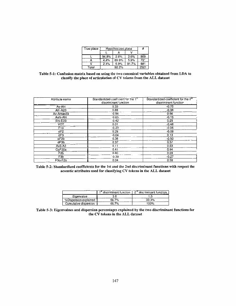
True place Hyp othesized >lace #L A V
L 94.8% 2.6% 2.6% 909A 4.4% 89.8% 5.9% 731V 2.4% 5.9% 91.7% 881
Total 92.2% 2521
Table 5-1: Confusion matrix based on using the two canonical variables obtained from LDA toclassify the place of articulation of CV tokens from the ALL dataset
Attribute name Standardized coefficient for the 1s Standardized coefficient for the 2"adiscriminant function discriminant function
Av-Ahi 0.33 -0.75Ahi-A23 0.88 -0.38
Av-Amax23 -0.94 0.56Avhi-Ahi -0.05 -0.15Ehi-E23 -0.42 0.29
VOT 0.01 -0.48Flo -0.23 -0.05dF2 0.28 -0.08dF3 -0.04 0.13
dF2b 0.38 -0.50dF3b 0.37 0.57
Av3-A3 0.11 0.53CgF20a 0.41 0.94
F2b 0.80 0.03F3b -0.39 -0.27
F3o-F2o 0.04 0.59
Table 5-2: Standardized coefficients for the 1st and the 2nd discriminant functions with respect theacoustic attributes used for classifying CV tokens in the ALL dataset
1i" discriminant function 2r" discriminant function
Eigenvalue 3.0 1.5%Dispersion explained 66.7% 33.3%Cumulative dispersion 66.7% 100%
Table 5-3: Eigenvalues and dispersion percentages explained by the two discriminant functions forthe CV tokens in the ALL dataset
147

Attribute name Contribution to 1 st discriminant Contribution to 2nd discriminant Overall Contributionfunction functionAv-Amax23 16.5% 8.8% 14.0%
Ahi-A23 15.5% 6.0% 12.4%CgF20a 7.2% 14.9% 9.8%
F2b 14.0% 0.4% 9.5%Av-Ahi 5.8% 11.9% 7.8%dF3b 6.6% 9.1% 7.4%dF2b 6.6% 7.9% 7.1%
Ehi-E23 7.4% 4.7% 6.5%F3b 6.8% 4.2% 6.0%
Av3-A3 2.0% 8.4% 4.1%dF2 4.9% 1.2% 3.7%
F3o-F2o 0.7% 9.3% 3.6%Flo 4.0% 0.9% 2.9%VOT 0.3% 7.6% 2.7%
Avhi-Ahi 0.9% 2.4% 1.4%dF3 0.8% 2.1% 1.2%Total ]j 100.0% 100.0% 1 100.0%
Table 5-4: Contributions to the 1"t, the 2"d discriminant function, and the overall discriminationamong the three places of articulation of the acoustic attributes used for the CV tokens in the ALL
dataset
5.3 Contribution Analysis on VC tokens in the ALL dataset
The same analyses that were done in section 5.2 were repeated for the VC tokens in the
ALL dataset. The scatter plot of the two canonical variables is shown in Figure 5-2. The
confusion matrix resulting from the LOOCV based on these two canonical variables is
shown in Table 5-5. The corresponding classification accuracy is 88.6%. From the plot,
we can see that the first canonical variable separates labial stop consonants and velar stop
consonants apart. In this dimension, alveolar stop consonants are mixed with the other
two types of stop consonants. In the dimension corresponding to the second canonical
variable, alveolar stop consonants are then separated from the other two types of stop
consonants. The standardized canonical coefficients associated with the two canonical
discriminant functions for all of the acoustic attributes are shown in Table 5-6. The
largest contribution to the first canonical discriminant function is due to Av-Amax23.
Some of the acoustic attributes that also have large standardized canonical coefficients
for the first discriminant function include Ahi-A23, dF2, and Av-Ahi. For the second
canonical discriminant function, the biggest contribution comes from Av-Ahi. Av-
Amax23, which is the biggest contributor to the first discriminant function, also
contributes a lot to the second discriminant function. These two acoustic attributes are
148

responsible for more than half of the separation due to the second discriminant function.
There were no other acoustic attributes that contribute to the second discriminant function
at any level close to these two.
The eigenvalue is 2.2 for the first canonical discriminant function and 0.9 for the second
function. This 71.6% of the total separation is due to the first discriminant function, while
the second function is responsible for the rest, which is 28.4%.
The overall contributions to the place classification of VC tokens in the ALL dataset due
to all of the acoustic attributes are ranked in Table 5-8. Of the total separation achieved
by the two canonical variables, 25.4% comes from Av-Amax23. Av-Ahi and Ahi-A23
are the second and third biggest contributors, respectively. The three acoustic attributes
are used for describing the shape of the release bursts, and they contribute to more than
half of the separation from the 15 acoustic attributes used here. The acoustic attributes
that contribute the least are dF2b and F3b-F2b. Each of them contributes less than 1% of
the total separation. Unlike the CV case, the contributions of these two acoustic attributes
might not be very significant compared to the contribution of other acoustic attributes.
Also, the movement of the second and the third formant frequencies at the voicing offset
of the preceding vowels contributes more to the total separation than their counterparts
measured at the release bursts, which was opposite to the CV case.
149

Scatter plot of the two canonical variables from the ALL dataset5-
o Labialx Alveolar
4-x A Velar
x x xX~ W CX X
3- x xx XX x Xx~4~
2 XX A
090.0
UX
0 0 0U UP
8 - 4 -2 0 2 4 Canonical Variable 1
Figure 5-2: Scatter plot of the two canonical variables for VC tokens from the A LL dataset
True place H otheizdlace_ #____ A V
L 2.6% 25% 400A . . 437V 3.% 93 70 689
Total 88.6% 1526
Table 5-5: Confusion matrix based on using the two canonical variables obtained from LDA to
classify the place of articulation of VC tokens from the ALL dataset
150
oil=

Attribute name Standardized coefficient for the 1 s' Standardized coefficient for the 2"0discriminant function discriminant function
Av-Ahi 0.69 -1.06Ahi-A23 0.93 -0.08
Av-Amax23 -1.44 1.01Avhi-Ahi 0.15 -0.21Ehi-E23 -0.32 0.22
CLSDUR -0.11 0.00Flo -0.21 -0.01dF2 0.93 0.00dF3 0.22 0.30dF2b 0.04 -0.03dF3b 0.06 0.04
Av2-A2 -0.03 0.28F2o 0.48 -0.06F3o -0.19 0.44
F3b-F2b -0.02 0.05
Table 5-6: Standardized coefficients for the 1st and the 2nd discriminant functions with respect theacoustic attributes used for classifying VC tokens in the ALL dataset
1s' discriminant function 240 discriminant function
Eigenvalue 2.2 0.9%Dispersion explained 71.6% 28.4%Cumulative dispersion 71.6% 100%
Table 5-7: Eigenvalues and dispersion percentages explained by the two discriminant functions forthe VC tokens in the ALL dataset
Attribute name Contribution to 1 discriminant Contribution to 2nd discriminant Overall Contributionfunction functionAv-Amax23 24.9% 26.6% 25.4%
Av-Ahi 11.8% 27.9% 16.4%Ahi-A23 16.0% 2.2% 12.1%
dF2 16.0% 0.1% 11.5%F2o 8.3% 1.5% 6.4%F3o 3.2% 11.7% 5.6%
Ehi-E23 5.5% 5.9% 5.6%dF3 3.7% 8.0% 4.9%
Avhi-Ahi 2.6% 5.5% 3.4%Flo 3.6% 0.3% 2.7%
Av2-A2 0.5% 7.3% 2.4%CLS DUR 1.9% 0.1% 1.4%
dF3b 1.0% 1.1% 1.1%dF2b 0.6% 0.7% 0.6%
F3b-F2b 0.3% 1.2% 0.6%Total 100.0% 100.0% 100.0%
Table 5-8: Contributions to the 1Vt, the 2 "d discriminant function, and the overall discriminationamong the three places of articulation of the acoustic attributes used for the VC tokens in the ALL
dataset
151

Generally in both the CV and the VC cases, if we look at the contribution of all of the
acoustic attributes in their corresponding acoustic attribute subsets, we can notice that the
acoustic attributes that are used for describing the spectral shape of the release burst
contribute to the classification more than the ones describing the formant structures into
and out of adjacent vowels. This trend is still consistent with what we have observed in
the discriminating properties of the acoustic attributes individually, despite the interaction
among the acoustic attributes. In both the CV and VC cases, Av-Amax23 is indicated to
be the acoustic attribute that contributes the most to the total separation for this specific
dataset. Furthermore, Ahi-A23 and Av-Ahi also have rather large contributions in both
cases.
5.4 Contribution Analysis on CV tokens with known voicing
contexts
Table 5-9 (a) and (b) shows the overall contribution of the acoustic attributes used for
classifying CV tokens in the V and U dataset respectively. For the V dataset, which
contained CV tokens with voiced stop consonants, Ahi-A23 is the biggest contributor,
followed by Av-Amax23. The acoustic attribute with the biggest contribution to the
separation for the U dataset, in which CV tokens contained voiceless stop consonants, is
cgF20a, followed by Av-Amax23. While cgF20a topped the contribution ranking for the
voiceless case, it is second to the bottom in the voiced case. This indicates that the
information about the spectral energy concentration between the release bursts and the
voicing onsets of the following vowels is very useful in classifying the place of
articulation of the voiceless stop consonant, while it is not that crucial for the voiced case.
This might be explained by that there is usually more aspiration after the release bursts of
voiceless stop consonants, apart from the ones of some unaspirated voiceless stops, than
after the release bursts of voiced stop consonants. Thus, the information about the
aspiration, which contributes partly to the value of cgF20a, helps the place classification
of the voiceless CV tokens more than the voiced ones.
152

Another interesting acoustic attribute is VOT. As we have seen in the result for the ALL
dataset, VOT does not contribute much to the place classification when we do not have
the information on the voicing. Here, we can see that VOT is more useful when the
voicing of the stop consonants is known. In both the V and U cases, VOT moves upward
in ranking compared to the result from the ALL dataset. It contributes around 4% as
opposed to around 2% in the ALL case. This is not surprising, as we have pointed out the
significant difference in the values of VOT for the voiced and voiceless stop consonants.
So, the variation caused by the with-in group error should be reduced when stop
consonants with different voicing are separated. For the voiceless case, it seems that the
information on the movement of the second formant frequency does not provide as much
contribution to the place classification as in the voiced case. dF2 and dF2b rank among
the acoustic attributes with the lowest contribution in the voiceless case, while both
acoustic attributes together yield almost 20% contribution to the place classification in
the voiced case. dF3 is still the acoustic attribute that contributes the least to the place
classification.
V UAttribute name Overall Contribution
CgF20a 14.3%Av-Amax23 10.3%
dF3b 9.2%F2b 9.1%
Ahi-A23 8.3%F3b 7.3%F3o 6.7%F2o 5.4%
Av3-A3 5.1%Ehi-E23 4.8%Avhi-Ahi 4.2%Av-Ahi 4.1%VOT 4.0%dF2b 2.5%Flo 2.2%dF2 1.6%dF3 0.9%
153
Attribute name Overall ContributionAhi-A23 13.0%
Av-Amax23 11.9%dF2b 10.9%F2o 10.0%
Av-Ahi 7.5%Ehi-E23 6.9%
dF2 6.1%dF3b 5.3%
F3b-F2b 5.0%Av3-A3 4.9%
VOT 4.8%F3o 4.4%Flo 3.3%
Avhi-Ahi 2.3%CgF20a 2.1%
dF3 1.8%
(a) (b)
Table 5-9: The overall contribution to the total separation of the acoustic attributes used for CVtokens in (a) the V dataset and (b) the U dataset
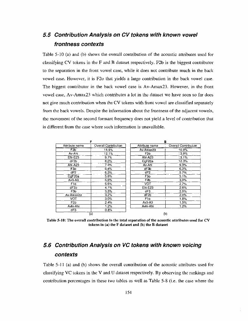
5.5 Contribution Analysis on CV tokens with known vowel
frontness contexts
Table 5-10 (a) and (b) shows the overall contribution of the acoustic attributes used for
classifying CV tokens in the F and B dataset respectively. F2b is the biggest contributor
to the separation in the front vowel case, while it does not contribute much in the back
vowel case. However, it is F2o that yields a large contribution in the back vowel case.
The biggest contributor in the back vowel case is Av-Amax23. However, in the front
vowel case, Av-Amax23 which contributes a lot in the dataset we have seen so far does
not give much contribution when the CV tokens with front vowel are classified separately
from the back vowels. Despite the information about the frontness of the adjacent vowels,
the movement of the second formant frequency does not yield a level of contribution that
is different from the case where such information is unavailable.
F BAttribute name Overall Contribution
F2b 14.8%Av-Ahi 12.1%Ehi-E23 9.7%dF2b 8.0%
Ahi-A23 7.3%F3o 6.8%dF2 6.3%
CgF20a 5.8%Av3-A3 5.6%
Flo 5.6%dF3b 4.1%F3b 3.5%
Av-Amax23 3.2%VOT 3.0%F2o 2.4%
Avhi-Ahi 1.2%dF3 0.8%
Attribute name Overall ContributionAv-Amax23 16.9%
F2o 13.9%Ahi-A23 13.1%CgF20a 12.3%Av-Ahi 9.3%dF3b 6.3%dF2 5.7%F3o 5.1%F2b 3.0%VOT 2.7%
Ehi-E23 2.6%dF3 2.5%
dF2b 2.0%Flo 1.8%
Av3-A3 1.5%Avhi-Ahi 1.2%
(a) (b)
Table 5-10: The overall contribution to the total separation of the acoustic attributes used for CVtokens in (a) the F dataset and (b) the B dataset
5.6 Contribution Analysis on VC tokens with known voicing
contexts
Table 5-11 (a) and (b) shows the overall contribution of the acoustic attributes used for
classifying VC tokens in the V and U dataset respectively. By observing the rankings and
contribution percentages in these two tables as well as Table 5-8 (i.e. the case where the
154

VC tokens of both voicings are mixed together), we can see that the relative contributions
of the acoustic attributes in each table are quite similar. Av-Amax23 contributes the most
to the total separation regardless of the voicing context. Also, regardless of the voicing
context, it is followed by Av-Ahi. Ahi-A23 and dF2 also contribute much in every
voicing context. And finally, the acoustic attributes at the bottom of these tables are
similar. They are CLSDUR, dF2b, and dF3b. It is also interesting to see that, although
the contribution percentages are not too different, the contribution of Ahi-A23 is less in
the voiceless case than in the voiced case and the nixed voicing case. This observation is
also true for the results obtained in the CV case.
V UAttribute name Overall Contribution
Av-Amax23 23.1%Av-Ahi 14.7%
dF2 11.1%Ahi-A23 9.0%
F3o 7.4%dF3 5.6%F2b 5.2%
Ehi-E23 4.4%Avhi-Ahi 4.1%
F2o 3.6%Flo 3.1%F3b 2.2%
Av2-A2 2.1%dF2b 2.1%dF3b 1.3%
CLS_DUR 0.9%
(a) (b)
Table 5-11: The overall contribution to the total separation of the acoustic attributes used for VCtokens in (a) the V dataset and (b) the U dataset
5.7 Contribution Analysis on VC tokens with known vowel
frontness contexts
Table 5-12 (a) and (b) shows the overall contribution of the acoustic attributes used for
classifying VC tokens in the F and B dataset respectively. Again, Av-Amax23 is the
biggest contributor regardless of the frontness of the vowels. For the front vowel case,
there are no drastic changes in the ranking when compared to the mixed vowel case,
except that the contribution of Ahi-A23 in the front vowel case is not as great as its
contribution in the mixed vowel case. It reduces from around 12% to around 7%. The
155
Attribute name Overall ContributionAv-Amax23 21.1%
Av-Ahi 15.3%Ahi-A23 14.9%
dF2 10.5%F2o 9.8%
Ehi-E23 5.3%F3o 4.8%dF3 4.6%
Av3-A3 3.6%Flo 2.7%
Avhi-Ahi 2.0%F3b-F2b 1.7%
dF3b 1.3%CLS DUR 1.2%
dF2b 1.1%

same thing is also true for the CV cases. For the back vowel case, the ranking looks
similar to the one in the mixed vowel case, except for the contribution of F2o. The
contribution of F2o is much smaller in the back vowel case than the mixed vowel case.
F BAttribute name Overall Contribution
Av-Amax23 20.0%dF2 13.9%
Av-Ahi 10.8%F2o 10.0%F3o 7.9%dF3 7.6%
Ahi-A23 7.4%Ehi-E23 4.8%
Flo 3.6%Av2-A2 2.4%
CLS DUR 2.3%F2b 2.3%
Avhi-Ahi 2.2%dF3b 2.1%F3b 1.9%
dF2b 1.0%
Attribute name Overall ContributionAv-Amax23 27.3%
Av-Ahi 15.6%Ahi-A23 13.8%
dF2 13.7%dF3 5.2%
Av3-A3 4.7%Ehi-E23 4.4%
Flo 3.5%F3o 2.3%
Avhi-Ahi 2.3%F3b-F2b 1.8%
dF2b 1.7%CLS DUR 1.3%
F2o 1.3%dF3b 1.2%
(a) (b)
Table 5-12: The overall contribution to the total separation of the acoustic attributes used for VCtokens in (a) the F dataset and (b) the B dataset
5.8 Summary on the Contribution to the Place Classification of
the Acoustic Attributes in Different Contexts
In the above sections, the contributions to the place of articulation classification of the
acoustic attributes used in different voicing and vowel frontness contexts were ranked. It
was clear to see that the acoustic attributes that contribution the most to the place
classification in most of the contexts was Av-Amax23. The contexts in which this was
not true were CV tokens with unvoiced stop consonants and CV tokens with front
vowels. In the former case, Av-Amax23 still contributed a lot to the classification but its
contribution was overshadowed by that of cgF20a, which was the acoustic attribute that
did very well for the place classification of unvoiced stop consonants. The latter case was
the only one where Av-Amax23 did not contribute much to the place classification.
While cgF20a, as just mentioned, was the biggest contributor to the place classification of
unvoiced stop consonants, it did not contribute much to the place classification of voiced
stop consonants. VOT, which did not seem to contribute significantly when voiced and
156

voiceless stop consonants were analyzed together, yielded a greater contribution when the
two types of stop consonants were classified separately. This was due to the difference in
the distributions of VOT of stop consonants with different voicing. Ahi-A23 always
contributed significantly regardless of the contexts, but its contribution was less in the
unvoiced and the front vowel cases for both CV and VC tokens.
In general, the effects of information about the voicing and the vowel frontness on the
contribution percentages and their ranking were smaller for the VC case than the CV
case. In the former case, the contribution percentages and the rankings did not change
much when the voiced and voiceless stop consonants were analyzed separately or when
the tokens with front vowels and back vowels were analyzed separately. What caused the
contribution percentages and ranking in the CV case to be affected by such information
more than the VC case was the presence of certain acoustic attributes whose value
distributions were expected to change significantly across different voicing and frontness
contexts. As mentioned, these acoustic attributes were VOT and cgF20a.
5.9 Chapter Summary
The main purpose of this chapter was to evaluate the relative importance of each of the
acoustic attributes for classification of the place of articulation of the CV and VC tokens
in nine datasets. Linear Discriminant function Analysis (LDA) was used. It reflected the
contribution of the acoustic attributes to the place classification in terms of the
standardized discriminant coefficients. We found slightly different levels of contributions
of the acoustic attributes used for the CV and the VC cases. In general, we found that in
the CV case, all of the acoustic attributes used were significant to the classification. In the
VC case, there were a couple of acoustic attributes that did not contribute much to the
classification relative to the amount of contribution of other acoustic attributes, and they
may be considered insignificant. For both cases, the acoustic attribute that contributes the
most was Av-Amax23. Also, the burst-related acoustic attributes showed more
contribution to the place of articulation classification than the formant-related ones. Some
of the acoustic attributes that did not separate the three places of articulation well
157

individually did contribute to the overall classification at some significant level. Also, the
contribution percentages of the acoustic attributes used in different voicing and vowel
frontness contexts and their rankings were listed. When the information about the voicing
of the stop consonant and the frontness of the vowel in each token was provided, the
contribution percentages and their ranking changed depending on the context. Some of
the changes were expected, while some were not obvious. The findings about the
contribution to the place classification of the acoustic attributes found in this chapter
should be useful in future attempts to customize the acoustic attribute subset to be used in
different contexts.
158
Chapter 6
Conclusion
6.1 Summary and Discussion
The main focus of this thesis is the study of the classification of stop consonant place of
articulation, which is performed in a knowledge-based fashion. The success in such a
knowledge-based classification will undoubtedly strengthen the idea of a knowledge-
based speech recognition system, which is believed by many researchers to be more
robust with regard to variations in its operating environment and which resembles human
speech recognition more than the traditional spectral-based and data-driven approach.
Acoustic attributes that have potential for discriminating stop consonant place of
articulation were chosen based on the simple tube model of stop consonant production,
described in Chapter 2. These acoustic attributes capture the information believed to be
relevant to the discrimination of the three places of articulation for English stop
consonants, i.e. labial, alveolar, and velar. This information includes the spectrum shape
of the release burst along with its amplitude relative to the adjacent vowels, the
movement of the formant frequency structure of the adjacent vowels, the frequency
concentration of the noise produced after the release of the stop closure, and some
temporal cues. These acoustic attributes were introduced along with their descriptions
and related measurement techniques in Chapter 3. Many of these acoustic attributes have
been used by different researchers for discriminating the place of articulation for stop
consonants with varied levels of success. Many of the earlier works in the literature
studied a limit number of acoustic attributes, while some of the more recent research tried
to utilize combinations of a larger number of acoustic attributes. While some of these
works reported the potential of using these acoustic attributes to classify stop consonants,
there is no extensive work on finding out the relative contribution of these acoustic
attributes to the separation of the three places of articulation.
159

In this thesis, the discriminating ability of each of the acoustic attributes in the selected
set was evaluated by observing the distributions of the values of each acoustic attribute
for the three places of articulation. Visually inspecting the box-and-whiskers plots
representing these distributions, which are shown in Chapter 3, one can qualitatively
assess how well each individual acoustic attribute separates the three places. The
significance of the differences among the distributions for the three places of articulation
was tested using ANOVA. The results showed that the differences in the distributions for
the three places in all of the acoustic attributes used in this study were statistically
significant. This indicates that the difference in the place of articulation is actually
reflected on how the value of each acoustic attribute is distributed. The relative values
among the three places of each acoustic attribute observed from the box-and-whiskers
plot was also compared with the relative values expected by the simple tube model. All of
the trends expected from each of the acoustic attributes for the three places were found to
be consistent with the observations from the box-and-whiskers plots. Still, there are some
findings related to the distributions of values of some acoustic attributes that have not
been fully explained in this thesis. Such findings should be investigated more extensively,
if one would like to learn more about their relations with the theory. Studies of this kind
should expand our state of understanding in human speech production. However, for the
purpose of this thesis, the observation of the distribution of values of each acoustic
attribute done in Chapter 3 has somewhat assured us that the measurements done in order
to obtain these acoustic attributes gave us what we expected from the theory.
The information about vowel frontness was found to alter the separabilities among the
three places of articulation of the acoustic attributes. Some acoustic attributes could
separate the three places better if the frontness of the vowels was known. This
encouraged us to take the vowel frontness context, along with the voicing context, into
account when the classification experiments were conducted in Chapter 4.
The degree of separation among the three places for each acoustic attribute was examined
using two quantifiers. The first one is the maximum likelihood classification error
probability based on the probability distributions of the values of each acoustic attribute
160

for the three places of articulation. These distributions were constructed by assuming
normal probability density functions, whose parameters were the associated sample
means and sample variances. The other quantifier is based on the F-ratio, which
represents the ratio between the amount of variation in the values of a particular acoustic
attribute that is caused by the place effect to the amount of variation caused by the
within-place error. These two quantifiers generally agree, i.e. an attribute that has a low
classification error probability usually has a high F-ratio, and vice versa. The abilities of
all of the acoustic attributes to separate the three places when each of the acoustic
attributes is used individually are ranked in Chapter 3 according to the associated
quantifiers. It was shown that both of the temporal attributes along with some of the
formant-related attributes were poor in separating the three places of articulation, while
all of the acoustic attributes that capture the spectral energy concentration after the
release burst and some of the burst-related attributes were among the best acoustic
attributes in discriminating among the three places. In general, the acoustic attributes that
capture the spectral shape of the release burst did better than the acoustic attributes that
capture the formant structure. Although many works in the literature, such as [Delattre,
Liberman, and Cooper, 1955], [Alwan, 1992], and [Foote, Mashoa, and Silverman,
1993], have emphasized the importance of formant movement, especially the second
formant, to the place classification of stop consonants, our results support the findings in
[Nossiar and Zahorian, 1991] and [Chen and Alwan, 2000], which state that the shape of
the burst spectrum is a more superior cue than the formant movement for classifying stop
consonants. A similar conclusion was stated by Ali [2001], who used combinations of
acoustic attributes to classify stop consonant and suggested that the role of formant
transitions is secondary to the burst spectrum. Despite this mentioned consistency with
other results in the literature, it is also possible that the inferiority of the formant-related
acoustic attributes might be the result of our choice of acoustic measurements used to
capture the formant information. Further studies could be done by introducing different
methods for capturing the formant movement, such as parametric representations of the
formant tracks. However, with the set of acoustic attributes used in this study, the
formant-related attributes, as well as the temporal cues, are clearly secondary to the burst-
related attributes.
161

In order to prevent redundant information contained among our acoustic attributes from
corrupting our further analyses and classification experiments, a correlation analysis was
performed in order to uncover possible redundant information. Some highly correlated
acoustic attributes were identified within various frontness and voicing contexts.
However, there was no evidence of cross-category highly correlated acoustic attributes.
Across all of the contexts, Av3-A3 and Av2-A2 were found to be highly correlated to
each other. This is not surprising due to the fact that both were calculated based on the
amplitudes of the biggest peaks in two overlapping arbitrary frequency regions. Given a
more accurate formant tracker, one could have chosen to use different acoustic attributes
that measure spectral amplitude directly at the second and third formant frequencies of
the release burst and the adjacent vowels. Specifically, Av3 and Av2 would be the
spectral amplitudes of the second and the third formant frequencies of the adjacent
vowels. And, similarly, A3 and A2 would be the spectral amplitudes of the two formant
frequencies of the release burst. However, despite the need for a good formant tracker to
measure these attributes automatically, the second and third formant frequencies could be
located manually just for the purpose of investigating their disciminating abilities. This
could be done in the future by using the same analysis techniques used in this thesis.
Another set of highly correlated acoustic attributes includes the formant-related attributes
that were measured at the voicing onset/offset of the adjacent vowels and at the release
burst where the stop consonants are voiced. This high correlation is due to the usually
short VOT of voiced stops. The fact that we have not found any evidence for cross-
category highly correlated acoustic attributes supports the common belief that robust
recognition can be achieved by combining cues from various sources, such as bursts and
formant transitions.
The result from the correlation analysis served as a tool to aid in the selection of subsets
of the acoustic attributes used for the classification experiments in Chapter 4. A set of
rules, based on the correlation coefficients of the acoustic attributes, was used to restrict
the number of all possible acoustic attribute combinations. Stop consonants with different
voicing and vowel frontness contexts were classified using all possible acoustic attribute
162

combinations, in order to find the highest classification accuracies. This acoustic attribute
selection is a 'filter' method performed on the same data that was used to obtain the
classification accuracy. Although it is not a fair way to evaluate the best attribute
combination for classifying unseen data, it allows us to evaluate the best classification
accuracies our acoustic attributes can achieve. Leave-One-Out Cross Validation
(LOOCV) technique was used to estimate the classification accuracies in all of the
classification experiments.
When stop consonants contained the release bursts, we could use the information about
release bursts along with other information in the classification, and that gave us the
classification accuracies that were mostly better than 90%. When stop consonants did not
contain the release bursts, the classification had to rely only on the information of the
formant structure of the adjacent vowels. The classification accuracies in this case were
not as high as the case where the release bursts were available. However, there were
some datasets that show rather good classification accuracies despite the lack of burst
information. It was also shown in Chapter 4 that training the CV classifier on the CV
tokens that had the same voicing and frontness contexts as the test tokens led to a better
classification accuracy than training on any general CV tokens forming the training set of
the same size. However, there was no evidence of significant classification accuracy
improvement for the VC case when the frontness and voicing contexts were used. This
implies that the place cues contained in the VC part are not as dependent on the frontness
and the voicing contexts as the cues in the CV part. There are more factors on which
some of our acoustic attributes are theoretically dependent. The classification accuracy
might be, and is likely to be, improved, if these factors are taken into consideration in
selecting the training data. An example of such factors is the [high] quality of the
adjacent vowel. This factor is directly relevant to the attribute Flo. Therefore, one would
expect the value distribution of Flo measured from tokens that are adjacent to high
vowels to be different from the one measured from tokens with non-high vowels.
Consequently, training the classifier on the data with the same [high] context as the test
tokens will possibly improve the classification result due to less variation in the Flo
dimension.
163
In the case of stop consonants that were located in between two vowels, we had the
advantage by being able to use information on the formant structures going into the
vowels on both sides. Two methods were used to classify such stop consonants separately
based on the information on their right side and left side. The probabilities of each place
of articulation proposed by the two classifiers were then combined in order to obtain one
final hypothesis about the place of articulation. Such a combination yielded the best
classification accuracy of 95.5%.
Apart from the classification accuracy from the combined classifiers, this experiment also
provided us with the classification accuracies obtained from using the information from
the VC part and the one obtained from using the information from the CV part evaluated
on the same dataset, i.e. stops that have vowels on both sides. When all of the cues, both
burst-related and formant-related, were used, we found that using the CV information
yielded a better classification accuracy than using the VC information, and the difference
is statistically significant. This shows that the information generated during the process of
moving into the following vowel is more reliable than the one out of the preceding vowel,
given that burst information is included in both cases. And when the VC and CV
classifiers disagree on the place of articulation of a stop consonant, most of the time our
combined decision favors the CV decision. This behavior is consistent with the findings
in many of the studies of place assimilation in stop consonant clusters [Fujimura, Macchi,
and Streeter, 1978][Dorman, Raphael, and Liberman, 1979][Streeter, and Nigro,
1979][Ohala, 1990]. These studies have found that human listeners generally hear the
consonant of the CV part when the place cues for VC and CV are in conflict. Such a
scenario is similar to when we have disagreement on the decisions from the VC and CV
classifiers.
The notion of combining scores obtained from two classifiers, each using information on
a different side of the stop consonant, can be extended to multiple classifiers, taking in
different types of information. Multiple sources of information could be experimented
with. For example, one might be interested to see the combined classification result of
164

stops in VCV contexts, if we have several classifiers, one of which uses only the release
burst information, another uses the formant transition information on the right, and a third
one uses the formants on the left. This way, we have the flexibility in adjusting the
weights applied to the scores from individual classifiers. However, the performance of
each classifier might not be as good due to the reduction in the amount of information
provided to each classifier. This would also allow us to combine the scores from a
spectral-based classifier and a knowledge-based classifier together.
At the end of Chapter 4, we evaluated the classification accuracy on all of the qualified
stop consonants in the database. When a particular stop consonant was to be classified, its
associated contexts were taken into consideration. These contexts include the voicing of
that stop consonant, the frontness of the adjacent vowel, and the presence of the release
burst, as well as the presence of vowels preceding and following the stop. The acoustic
attribute subset and the training data used in the classification of each stop consonant
were selected based on these contexts. Stops that had vowels on both sides were
classified using the combined scores obtained from information on both sides. The place
of articulation classification accuracy of 92.1% was achieved. It was pointed out that the
overall classification accuracy could be improved significantly if stop consonants in VC
context with no release burst were classified more accurately. Although the stop
consonants involved in this classification are somewhat restricted, e.g. only the stop
consonant that has at least a vowel segment adjacent to it is included in this study, and
there are stop consonants that were intentionally left out due to significant gestural
overlapping, the achieved classification accuracy of 92.1% is still encouraging, given that
additional processing could be developed in the future to handle the left out cases. For
example, a flap detector could be developed in order to identify all of the flaps before
trying to determine the place of articulation.
Compared to the place classification accuracy of 85% for syllable-initial stops obtained in
[Stevens, Manuel, and Matthies, 1999], we achieve an approximately 8% higher
classification accuracy for stops regardless of syllable structure. In [Stevens, Manuel and
Matthies, 1999], six acoustic attributes, describing the spectral shape of the release burst
165

along with some formant transitions, were used with a statistical classification method
similar to the one used in this study to classify syllable-initial stops. In this study, we
used approximately seventeen acoustic attributes, including the six attributes used in
[Stevens, Manuel and Matthies, 1999], to classify stop consonants in broader contexts.
The frontness information was used in [Stevens, Manuel and Matthies, 1999], while, in
this study, we also used the voicing information. The improvement gained was mainly
due to the introduction of additional acoustic attributes, which allowed more of the
relevant information to be captured.
Hasegawa-Johnson [1996] used 10 acoustic attributes in context-dependent place
classification, which resulted in 84% classification accuracy. Direct comparison should
not be made on the classification accuracies due to the difference in the database used.
Still, it is worth noting the difference in utilizing context information. Hasegawa-Johnson
used 36 different context classes, including all possible combination of 2 genders and 18
right contexts, while we used contexts in a broader sense, i.e. voicing of the stops and
vowel frontness. The fact that Hasegawa-Johnson used a large number of context classes
leads to a lack of generalization of the training data, and the need for considerably more
training materials hampers the classification accuracy. Also, both in [Hasegawa-Johnson,
1996] and in [Stevens, Manuel, and Matthies, 1999], the acoustic attributes used for each
context class were fixed, while in our study here, we have found in the attribute subset
selection in section 4.1.1 that using different acoustic attribute subsets led to different
accuracies, although not all of the acoustic attribute combinations gave significantly
different classification accuracies.
In [Ali, 2001], the place classification accuracy obtained is 90%. There are both different
and similar aspects between [Ali, 2001] and our work. Although the exact measurements
from the speech signal are different, both studies generally used rather similar
information on the spectral shape of the release burst, formant transitions, and some
temporal cues, as well as the frequency of the noise in the release burst region. In this
study, this information is contained in the acoustic attributes that were used as the
classification vector of a statistical classifier, while in [Ali, 2001], the information is used
166

for making decisions in a decision tree with hard thresholds, also learned from the
training data. Despite the difference, both methods of classification can be considered
knowledge-based methods and the resulting parameters in both classifier models, i.e. the
thresholds and the positions of decision nodes in the decision tree, and the canonical
weights used in the corresponding analyses in our study, should help improve our
understanding of the acoustic-phonetic characteristics of the stop consonants. Such a
benefit is hard to obtain, if at all possible, from a spectral-based data-driven approach.
Some of the stop consonants found in the transcription of the utterances in the SP
database were left out of the classification in this study, according to the restriction
described in section 3.1. The number of these excluded stops is around 35% of the total
number of stops in the database. As mentioned, for the qualified stops, which are around
65% of the total, the classification accuracy obtained is 92.1%. Therefore, if the
classification accuracy of the excluded set can be obtained, the overall classification
accuracy for all of the stops in the SP database can be calculated. Figure 6-1 shows the
total classification accuracy as a function of the accuracy obtained from classification of
the excluded stops. If we can perfectly identify the place of all of the excluded stops, the
total classification accuracy of 94.8% will be obtained. It is reasonable to say that this is
hardly possible. The reason is that the place classification of some of the excluded stops
should be more problematic than the qualified stops due to high level of gestural overlap
and the lacking of formant structure information. Although it is relatively easy to detect
flaps [Ali, 2001], whose associated places are alveolar, flaps constitute only a small
fraction of the excluded set compared to stops that do not have any adjacent vowels.
Therefore, obtaining perfect classification on the excluded set should not be a reasonable
expectation. On the other hand, if we misidentify all of the places for the excluded stops,
the total classification accuracy will be as low as 60.1%. In order to obtain the total
classification accuracy of 93.3%, which was reported by Halberstadt [1998] as human
performance in place classification of stop consonants, we should expect a classification
accuracy of 96.3% for the excluded set, which is again higher than what we have
achieved for the qualified stops. This implies that there is still some room for
167

improvement on our classification method in order for the classification accuracy to meet
the human level.
100
95
90
85
80
0
75
70
L65F
60K --
94.8%
93.3%
_ _ _ _ 1% 96.3%
0 10 20 30 40 50 60 70 80classification accuracy on the left out stops (%)
90 100
Figure 6-1: Relationship between the classification accuracy of stops in the entire SP database andthe classification accuracy of the excluded stops
Finally, in Chapter 5, the relative importance of each of the acoustic attributes used the
place of articulation classification of the CV and VC tokens, when combinations of these
acoustic attributes were used, was evaluated by means of Linear Discriminant function
Analysis (LDA). The voicing and vowel frontness contexts were taken into consideration
in the analyses. Standardized discriminant coefficients reflected the contribution of the
acoustic attributes to the place classification. We have found that in the CV case, all of
the acoustic attributes used were significant to the classification. However, in the VC
case, there were some acoustic attributes that did not contribute much to the classification
relative to the amount of contribution of other acoustic attributes. These acoustic
168
- -

attributes may be considered insignificant and can be omitted without sacrificing a great
deal of classification accuracy.
For both cases, the acoustic attribute that contributes the most was Av-Amax23. Also, the
burst-related acoustic attributes showed more contribution to the place of articulation
classification, using these specific acoustic attribute subsets, than the formant-related
ones. This is consistent with discriminating ability of each individual burst-related and
formant-related attribute, which has been mentioned earlier. Some of the acoustic
attributes that did not separate the three places of articulation well individually did
contribute to the overall classification at some significant levels. The contribution
rankings varied by the voicing and vowel frontness contexts, and some of the ranking
discrepancies in different contexts can be simply explained by acoustic-phonetic
knowledge. Therefore, this shows that, given certain contexts, one can use acoustic-
phonetic knowledge to identify the relative importance of the acoustic attributes a priori.
The relative importance should serve as a guideline for choosing the appropriate sets of
acoustic attributes for the place classification of stops in those contexts.
6.2 Contributions
Experimental data of the acoustic attributes
This study provides experimental data on the distributions of the acoustic attributes for
the three places of articulation. The distributions among the three places of articulation
show consistency with the expectations formulated from the simple tube theory. One can
also observe these acoustic measurements more extensively to gain more understanding
about human speech production process. Furthermore, labeled with their corresponding
segments, the associated time points in their corresponding utterances, as well as some of
the contexts, these acoustic measurements can be used in studying other aspects of stop
consonants, such as voicing and some characteristic of flaps.
169

Quantitative measurements of the discriminating abilities of the acoustic attributes
Two quantifiers used in this study show that the center of gravity of the power spectrum
of the noise after the release burst shows the greatest degree of separability among the
three places of articulation in both CV and VC contexts. Also, acoustic attributes that
carry information about the release burst can separate the three places more than the ones
that carry the formant structure information. This finding agrees with some of the studies
in the literature, (at least in the absence of noise).
Stop consonant place of articulation classification results
This study provides experimental results on various classification of stop consonant place
of articulation using combinations of acoustic attributes. We estimate the classification
accuracies that can be achieved by using a knowledge-based method. The finding is
encouraging in terms of the achieved accuracies, although stops in broader contexts
should be studied and handled in the future. It also shows the importance of the voicing
and vowel contexts to the classification accuracy. Furthermore, this study also underlines
the possible improvement in classification accuracy when classifiers are aware of various
contexts of each stop consonant.
Results on the contributions of different acoustic attributes to the separation of the three
places of articulation
When combinations of acoustic attributes are used for the classification, Av-Amax23 is
among the biggest contributors to the classification results across almost all of the
voicing and vowel frontness contexts. And the fact that the burst-related acoustic
attributes show more contribution to the place of articulation classification than the
formant-related ones strengthens the claim that release bursts are more crucial to the
identification of stop place than formant transitions. The discrepancies in the ranking of
different contexts emphasized the need for taking contexts into consideration in choosing
appropriate acoustic attributes.
170

Exploratory framework for determining the value of distinctive features
The series of statistical analyses performed in this study can be applied to the study of
other classes of sounds, or stops in different noise conditions. For example, if one wishes
to study different sets of acoustic attributes for determining place of articulation for
fricatives, or for detecting nasals from other classes of sounds, it could be a good practice
to observe the value of each acoustic attribute and evaluate its ability to do the desired
task. Then, one might want to learn about redundant information and avoid highly
redundant attributes before performing classification experiments using appropriate
combination of acoustic attributes. Finally, to gain more insights about the contribution of
each acoustic attribute, LDA could be used. Other techniques might be applied to study
the role of each acoustic attribute further. Some of the techniques that should give extra
insights about this include Principle Component Analysis (PCA), and Artificial Neural
Networks (ANN).
6.3 Future Work
The utterances in the database used for this study were recorded in a quiet room. The
discriminating ability of each acoustic attribute, the classification accuracies, and the
contribution of each acoustic attribute to the classification accuracy were determined
under a clean speech condition. It is of interest to see how these change in the presence of
noise, since one of the benefits of the knowledge-based approach to automatic speech
recognition is that the attributes used for determining the underlying sounds are
meaningful, and one could use the knowledge to manipulate these attributes according to
the operating environment. For example, the burst-related attributes, which were shown
to separate the three places of articulation better than the formant-related ones in the
clean speech condition, might not be as useful for the classification if some of the
features in the burst spectrum that are important in determining the burst-related
attributes are overwhelmed or masked by noise. Figure 6-2 shows two spectrograms of
the same utterance with two different noise conditions. The top spectrogram is obtained
without added noise, while the bottom one is obtained from the signal that is mixed with
171

white noise at 28dB Signal-to-Noise Ratio (SNR) 3. The movement of the first three
formants can mostly still be determined even in the presence of this noise. However, most
of the high frequency region of the release bursts is masked by the noise, at least for the
simple spectral analysis used for making the spectrogram. Therefore, in this particular
noise condition, one would expect the burst-related attributes that require measurements
in the high frequency region to lose some of their discriminating ability, unlike the
formant-related attributes that seem to be unaffected by the noise in this particular case.
Figure 6-3 is a plot of some preliminary data showing the degradations of the
discriminating ability of two burst-related acoustic attributes, which are Av-Ahi and Av-
Amax23, in white noise at different SNR levels. Both attributes show rather similar
discriminating abilities in clean speech. However, Av-Amax23 does not degrade much in
the noisy condition of up to 25dB SNR, but Av-Ahi shows a greater level of degradation
in the same noisy condition due to the corrupted Ahi. This data shows that the relative
importance of each acoustic attribute in classifying place of articulation changes with
noise condition. Thus, applying a methodology similar to that presented in this study to
speech in different types of degradation, e.g. speech different types of noise, speech in
reverberation, and more casual speech, should be useful in both the development of a
better stop place classification module and the understanding of human perception of stop
consonant place of articulation.
3 Here, the Signal-to-Noise Ratio is the ratio between the RMS peak of the signal of interest and the
standard deviation of the white noise.
172
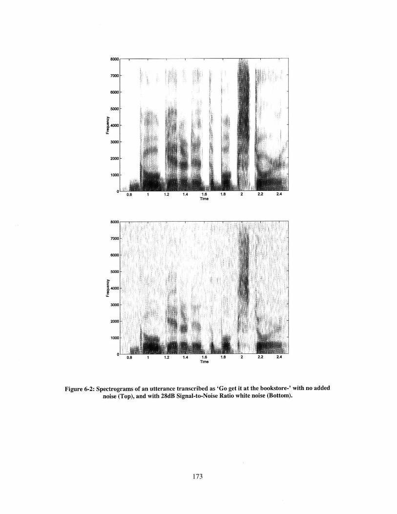
7000 -
10000
5000
S4000-
2000-
1000 -
0 0.8 1 1.2 1.4 1.6, 1.8 2 2.2 2.4Time
8OOC
7000
6000
5000 -
4000 -
3000 -
2000 -
I OW -
0 0.8 1 1.2 1.4 1.6 1.8 2 2.2 2.4Time
Figure 6-2: Spectrograms of an utterance transcribed as 'Go get it at the bookstore-' with no addednoise (Top), and with 28dB Signal-to-Noise Ratio white noise (Bottom).
173
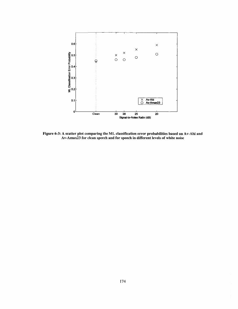
0.6-
xx
~0.5 -Q
B9 004 0 00
2 0.4 -020.32
C.)-0.2
0.1- X Av-Ahi0 Av-Amnax.23
0,Clean 30 28 25 20
Signal-to-Noise Ratio (dB)
Figure 6-3: A scatter plot comparing the ML classification error probabilities based on Av-Ahi andAv-Amax23 for clean speech and for speech in different levels of white noise
174

Biblography
Ali, A.M.A., J.V. Spiegel, and P.Mueller, "Robust classification of stop consonants using
auditory-based speech processing", ICASSP, Salt Lake City, May, 2001
Ali, A.M.A., J.V. Spiegel, P. Mueller, G. Haentjens, and J. Berman, "Acoustic-Phonetic features
for the automatic classification of stop consonants", J. Acoust. Soc. Am., Vol.103(5),
pp.2777-2779, 1998
Alwan, A.A., "Modeling speech perception in noise: The stop consonants as a case study", Ph.D.
Thesis, MIT, 1992
Blumstein, S., and K.N. Stevens, "Acoustic invariance in speech production: Evidence from
measurements of the spectral characteristic of stop consonants", J. Acoust. Soc. Am.,
Vol.66(4), pp.1001-1017, 1979
Bonneau, A., L. Djezzar, and Y. Laprie, "Perception of the Place of Articulation of French Stop
Bursts", J. Acoust. Soc. Am., Vol.1, pp.555-564, 1996.
Chen W. S., and A.A. Alwan, "Place of Articulation Cues for Voiced and Voiceless Plosives and
Fricatives in Syllable-Initial Position", proc. ICSLP 2000. Vol. 4, pp. 113-116, 2000.
Chen, M.Y., "Nasal detection model for a knowledge-based speech recognition system", proc.
ICSLP2000, Vol.4, Beijing, China, pp.636-639, 2000
Choi, J., "Detection of consonant voicing: A module for a hierarchical speech recognition
system", Ph.D. Thesis, MIT, 1999
Chomsky, N., and M. Halle, "The sound pattern of English", Harper & Row, New York, 1968
Chun, R., 'A hierachical feature representation for phonetic classification", M.Eng. Thesis, MIT,
1996
Davis, S.B., and P. Mermelstein, "Comparison of parametric representations for monosyllabic
word recognition in continuously spoken sentences", IEEE Trans. Acoust. Speech, Signal
Processing, Vol. ASSP-28(4), pp.257-366, 1980
175
Delattre, P.C., A.M. Liberman, and F.S. Cooper, "Acoustic loci and transitional cues for
consonants", J. Acoust. Soc. Am., Vol.27, pp.769-773, 1955
Dorman, M.F., L.J. Raphael, and A.M. Liberman, "Some experiment on the sound of silence in
phonetic perception", J. Acoust. Soc. Am., Vol.65, pp.1518-1532, 1979
Engstrand, 0., D. Krull, and B. Lindblom, "Sorting stops by place in acoustic space", Proc. the
XIIIth Swedish Phonetics Conference (FONETIK 2000) Skivde, Sweden, pp.53-56, May,
2000
Fisher, R.A., "The use of multiple measurements in taxonomic problems", Annals of Eugenics
London, Vol. 7, pp. 179-188, 1936
Foote, J. T., D. Mashao, and H.F. Silverman, "Stop classification using desa-] high-resolution
formant tracking", proc. ICASSP, Vol.2, pp.720-723, April 1993
Fujimura, 0., M.J. Macchi, and L.A. Streeter, "Perception of stop consonants with conflicting
transitional cues: A cross-linguistic study", Language and Speech, Vol.21, pp.337-346, 1978
Fukunaga, K., "Introduction to statistical pattern recognition", Academic Press Inc., San Diego,
CA, 1990
Gidas, B., and A. Murua, "Classification and clustering of stop consonants via nonparametric
transformation and wavelets", proc. ICASSP, Vol.1, pp. 872-875, 1995
Halberstadt, A.K., "Heterogeneous acoustic measurements and multiple classifiers for speech
recognition", Ph.D. Thesis, MIT, 1998
Hall, M.A., "Correlation-based feature selection for machine learning ", Ph.D. thesis, University
of Waikato, New Zealand, 1999
Hasegawa-Johnson, M.A., "Formant and burst spectral measurements with quantitative error
modelsfor speech sound classification", Ph.D. Thesis, MIT, 1996
Hermansky, H., and N. Morgan, "RASTA processing of speech", IEEE trans. on speech and audio
processing, Vol.2(4), October, 1994
Howitt, A.W., "Automatic syllable detectionfor vowel landmarks ", Ph.D. thesis, MIT, 2000
176

Jakobson, R., C.G.M. Fant, and M. Halle, "Preliminaries to speech analysis: The distinctive
features and their correlates", MIT Acoustic Laboratory Technical Report 13, MIT Press,
Cambridge, MA, 1967
Jankowski Jr., C.R., H.V. Hoang-Doan, and R.P. Lippman, 'A comparison of signal processing
front ends for automatic word recognition", IEEE Trans. Speech Audio Processing, Vol.3,
pp.286-293, July, 1995
Johnson, K., "Acoustic and auditory phonetics", Blackwell Publishers Inc., Cambridge, MA,
1997
Johnson, R. A., "Miller & Freund's Probability & Statistics for Engineers", Prentice Hall, New
Jersey, 1993
Kent, R.D., and C. Read, "The acoustic analysis of speech", Singular Publishing Group Inc., San
Diego, CA, 1992
Kewley-Port, D., "Time-varying features as correlates of place of articulation in stop
consonants", J. Acoust. Soc. Am., Vol.73(1), pp.322-335, 1983
Kingsbury, B., N. Morgan, and S. Greenberg, "Robust speech recognition using the modulation
spectrogram", Speech Communication 25, pp. 117-132, 1998
Koreman, J., B. Andreeva, and H. Strik, 'Acoustic parameters versus phonetic features in ASR",
proc. ICPhS'99, Vol.1, San Francisco, pp.7 19-722, 1999
Lahiri A., L. Gewirth, and S. Blumstein, "A reconsideration of acoustic invariance for place of
articulation in diffuse stop consonants: Evidence from a cross-language study", J. Acoust.
Soc. Am., Vol.76, pp.3 9 1-404, 1984
Lee, K.F., 'Automatic speech recognition: The development of the SPHINX system", Kluwer
Acedemic Publishers, Norwell, MA, 1989
Levelt, W.J.M., A. Roeloff, and A. Meyer, "A theory of lexical access in speech production",
Brain and Behavioral Sciences 22, pp.1-75, 1999
Lindman, H. R., 'Analysis of variance in complex experimental designs", W. H. Freeman & Co.,
San Francisco, 1974.
177
Liu, S.A., "Landmark detection for distinctive feature-based speech recognition", Ph.D. thesis,
MIT, 1995
Malbos, F., S. Baudry, and S. Montresor, "Detection of stop consonants with the wavelet
transform", IEEE-SP, International Symposium on Time-Frequency and Time-Scale
Analysis, Philadelphia, USA, pp. 612-615, 1994
Manly, B.F.J., "Multivariate Statistical Methods: A primer", Chapman and Hall Ltd., New York,
NY, 1986
Massey, N.S., "Transients at stop-consonant release", S.M. thesis, MIT, 1994
Nathan, K.S., and H.F. Silverman, "Time-varying feature selection and classification of unvoiced
stop consonants", IEEE trans. Speech and Audio Processing, Vol.2, No.3, pp.395-405, 1994
Nossiar, Z.B., and S.A. Zahorian, "Dynamic spectral shape features as acoustic correlates for
initial stop consonants", J. Acoust. Soc. Am., Vol.89(6), pp.2978-2991, 1991
Ohala, J.J., "The phonetics and phonology of aspects of assimilation", In Kingston J., and
Beckman M. (eds.), Papers in Laboratory Phonology, Vol.1, Cambridge University Press,
Cambridge, UK, pp.258-275, 1990
Rabiner, L., and B.H. Juang, "Fundamentals of speech recognition", Prentice-Hall Inc., New
Jersey, 1993
Repp, B., and H. Lin, "Acoustic properties and perception of stop consonants release
transients", J. Acoust. Soc. Am., Vol.85(1), pp.379-396, 1989
Searle, C.L., J.Z. Jacobson, and S.G. Rayment, "Stop consonant discrimination based on human
audition", J. Acoust. Soc. Am., Vol.65, pp.799-809, 1979
Stevens, K.N., "The quantal nature of speech: Evidence from articulatory-acoustic data", In P.B.
danes and E.E. Davids Jr. (eds.), Human Communication: A Unified View, McGraw-Hill,
New York, pp.5 1-66, 1972
Stevens, K.N., "Acoustic Phonetics", MIT Press, Cambridge MA, 1998
Stevens, K.N., "Toward a model for lexical access based on acoustic landmarks and distinctive
features ", J. Acoust. Soc. Am., Vol.111, pp.1872-1891, April, 2002
178

Stevens, K.N., S.Y. Manuel, and M. Matthies, "Revisiting place of articulation measuresfor stop
consonants: Implications for models of consonant production", proc. ICPhS'99 Vol.2, San
Francisco, pp.1117-1120, 1999
Streeter, L.A., and G.N. Nigro, "The role of medial consonant transitions in word perception", J.
Acoust. Soc. Am., Vol.65, pp.1533-1541, 1979
Sun, W., 'Analysis and interpretation of glide characteristics in pursuit for an algorithm for
recognition", S.M. Thesis, MIT, 1996
Sussman, H.M., H.A. McCaffrey, and S.A. Matthews, "An investigation of locus equations as a
source of relational invariance for stop place categorization", J. Acoust. Soc. Am.,
Vol.90(1), pp.1309-1325, 1991
Timm, N. H., "Applied Multivariate Analysis", Springer Texts in Statistics, Springer-Verlag New
York Inc., New York, NY, 2002
Webb, A., "Statistical Pattern Recognition", John Wiley & Sons Ltd., West Sussex, England,
2002
Winitz, H., M. Scheib, and J. Reeds, "Identification of stops and vowels for the burst portion of
/p,t,k/ isolatedfrom conversational speech", J. Acoust. Soc. Am., Vol.51(4), pp.1309-1317,
1972
Zue, V., "The use of speech knowledge in automatic speech recognition", proc. of the IEEE,
Vol.73(11), pp.1602-1614, November, 1985
Zue, V., and R. Cole, "Experiments on spectrogram reading", Proc. ICASSP, pp. 1 16-119,
Washington, D.C., 1979
Zue, V., J. Glass, A. Philips, and S. Seneff, "The MIT SUMMIT speech recognition system: A
progress report", proc. DARPA speech and natural language workshop, Philadelphia,
pp.179-189, February 1989
Zue, V.W., "Acoustic characteristic of stop consonants: A controlled study", Sc.D. thesis, MIT.
1979
179

Appendix A
Sentences in the SP database
Pat ate it all upTo cope with the pain, Garcia dopes with a whole pack of painkillersBob should buy the two big booksA bug sped across the table and ended up in the jugLook at the cute boy with a bagThat spiky head geek likes to put beads around his right legPete and Abe had a bad day todayCopy cats cause the state cops a lot of headacheA big dog bit a dead duck at the gateThe logo was put on all of Bob's company's mugs, cups and bowlsA guard at the gate is going to get all the baggagePeggy has a piece of cake with a bottle of cokeDobbie caught a lot of bees and bugs but not any dovesKate hit a gecko by the pool with her bagPeggy and Rebecca go gambling with Pat in VegasDo not let the bed bugs bite the boysGo put on gold lipstick, get a hip skirt, and dye your hair pinkA gold beetle bug logo is too good for PeggyBecky took her puppy to Malibu two days agoThe red dot on that map locates where Dudley station isTaking a cab to Pawtucket could cost eighty bucksDobbie beats that poor boy for stepping on her toeBo bought a lot of goodies, but Gary bought only a geeky looking mugCould Ted have a pack of Thai tea?Despite its appearance, you need some guts to get this job donePut a black dot and a red tick on the tea-pot at the gateThe jug is made of stone but the mug is a skullTodd did not take the key but he took the kiteA bunch of bugs in Garcia's code could kill the whole systemStop digging. It's too deep alreadyThe kids are looking at a couple of beautiful kites in the skyKoby adds some peas and an egg into the stone potCould we book tickets to Cuba, Ghana and Tibet?Bob and Bo go to beg Gary to give them the gold bugYou can take the cookies and the cake but do not eat the pieThe tool kit keeps beeping due to the coke stainThe kids hit that duck with their bootsGarcia is recording beautiful pop music played by a big bandWhere did you go with Kate last autumn? Malibu, Pawtucket or Cape Cod?The blood from the goose's leg is dripping into the test tubeDick wishes he could step into the cockpit of his toy robotDo Bob and Dobbie take that cop to the dock?Katie poked a poor gibbon with a pikeThis kind of cake is too tough for Koby to bakeInstead of that Prada golden bag, Garcia gave a Gucci bag to GoldieDad does not eat an egg pie because it gives him a stomach acheDobbie and Debbie have gone to Cuba and have not come backA cop came and towed away Beck's white truckA toy toad was tied to a test tube in Debbie's labKitty the cat put her paw into the bowl of cookie doughThat guy looked a bit odd, and so did his kidGod likes a guy who does good deedsPopular types of toys have been out of stock for a couple of weeksDye that egg pink and put it in the kettle on that teak tableThat little puppy eats like a big pigBo goes to Ghana to catch a gold bugPat's daughters bike all day and jog all nightA goose takes a pack of peanuts out of Beck's pocketBob should look up how to cook the potpie in his cookbookA cop caught Ted stealing a box of doughnuts from the storeGo grab some goodies from the Gucci store, and do not forget the bagPeggy pays for the pigs and the goats with the beads
180

Tapping on the side of that cube will open up a big gap on its topWhile the gibbon was smoking his pipe on the dock, the gecko took the stolen boatDid you go to Cape Cod by car, bike or boat?The hawk put its beak into the bucketEighty two ducks are resting on that muddy bankGoldie got two good mugs as a gift from PeggyDucks and geese could be pets but pigs should notPeggy bought her kids a bucket of cookies and two bottles of cokeRobots and cars are popular toys among little boysAny good cops can cope with the case that happened at the top of the hubPat's cooking is so bad that her food makes Pete pukeA speed boat hit a rock and sank into the bottom of the bayAn ape picked up a dead bat by the poolKids cannot stay in bed all day longKoby put a big logo on the podium in his pubDebbie's kid hides his muddy boots in his backpackA Thai guy got into that big store a while agoTwo tired goats were found in the cockpitToday is a bad day to go apple pickingTodd has gone to Malibu since the last OctoberDo not forget the code for the front door when you come backLet's go to the pub in the odd side of the townGo and pick some peaches by the pool for the fruit pieGreg caught a full bucket of cod by using an odd type of baitBeck tightens the band around the big toy boxA stupid guy said that a cock could lay eggsThe boat was stored in the cabin by the dockGibbs and Gary beg Peggy to find bugs in their codeTake two buckets to the tap in front of the gateWhy did Abe put that cap in the cubic package?Dick is too uptight to let himself be happyIs Sapporo popular for its hot tubs?Beck taught his daughter how to play with a kiteKatie puts the tips into the big cup on that oak tableBandit robs the cookie store next to the pubBecky and the boys have finished packing their bags for the Cape Cod tripAll of the boats in the bay were brought back to the docksA total of sixty goats were on the dock todayDo not dump the gecko until you get to GhanaTodd tips Pete to play pool at the pub and get paidAbe acted like a boy when he did a bad deedThat geek is paid big bucks to build that hi-tech toolThe dog with a black dot on the tip of its tail is digging a deep holeA pack of cokes was put on the podium by some bad kidsGo get it at the bookstore, not at the pubThis type of kit is odd and out-of-dateBob got Katie a good book about a spooky goat in TibetThe code was published in that book a decade ago
181