Journal of Structural Biology 174 (2011) 494–504

Contents lists available at ScienceDirect

Journal of Structural Biology

journal homepage: www.elsevier .com/ locate/y jsbi

Classification of electron sub-tomograms with neural networks and its applicationto template-matching

Zhou Yu, Achilleas S. Frangakis ⇑Frankfurt Institute for Molecular Life Sciences and Institute of Biophysics, Goethe University Frankfurt, Max-von-Laue Str.1, 60438 Frankfurt am Main, Germany

a r t i c l e i n f o a b s t r a c t

Article history:Received 16 December 2010Received in revised form 25 February 2011Accepted 28 February 2011Available online 5 March 2011

Keywords:Sub-tomogram classificationImage processingCryo-electron tomography

1047-8477/$ - see front matter � 2011 Elsevier Inc. Adoi:10.1016/j.jsb.2011.02.009

⇑ Corresponding author.E-mail address: achilleas.frangakis@biophysik.org

Classification of electron sub-tomograms is a challenging task, due the missing-wedge and the low signal-to-noise ratio of the data. Classification algorithms tend to classify data according to their orientation to themissing-wedge, rather than to the underlying signal. Here we use a neural network approach, called theKernel Density Estimator Self–Organizing Map (KerDenSOM3D), which we have implemented in three-dimensions (3D), also having compensated for the missing-wedge, and we comprehensively compare itto other classification methods. For this purpose, we use various simulated macromolecules, as well astomographically reconstructed in vitro GroEL and GroEL/GroES molecules. We show that the performanceof this classification method is superior to previously used algorithms. Furthermore, we show how thisalgorithm can be used to provide an initial cross-validation of template-matching approaches. For theexample of sub-tomogram classification extracted from cellular tomograms of Mycoplasma pneumoniaand Spiroplasma melliferum cells, we show the bias of template-matching, and by using differing searchand classification areas, we demonstrate how the bias can be significantly reduced.

� 2011 Elsevier Inc. All rights reserved.

1. Introduction

Cryo-electron tomography (CET) provides unique three-dimen-sional (3D) images of cells and organelles at molecular resolution.The application range varies from tissue and whole cells to organ-elles and large pleiomorphic in vitro samples like viruses (Leiset al., 2009; Li and Jensen, 2009; Milne and Subramaniam, 2009).Ultimately, CET aims to visualize the spatial organization andinteraction of various macromolecules in the cellular context. Cur-rently, most of the applications are based on multiple occurringstructures, which are averaged in order to improve the resolution(Al-Amoudi et al., 2007; Beck et al., 2004; Briggs et al., 2009). Thus,sub-tomogram averaging and classification techniques play anessential role in data interpretation.

A number of classification methods have been presented overthe last years, all of which were inspired by their counterparts usedin single-particle electron microscopy. For the purpose of tomogra-phy, where the signal already exists in 3D, the classification aims toidentify populations of macromolecules with different conforma-tions and various interaction partners. In addition, an emergingapplication is classification of the sub-tomograms and separationof the selected sub-tomograms into true and false-positives hitsafter the application of template-matching algorithms. True-posi-tive hits are positions selected from the template-matching that

ll rights reserved.

(A.S. Frangakis).

correspond to the sought macromolecule, and false-positive hitsare those that do not correspond to the sought macromolecule,but rather represent other features such as membranes or debris.Template-matching algorithms use a template which is translatedand rotated in 3D space and its similarity is measured locallyagainst each position in a tomogram (Frangakis et al., 2002). Final-ly, at every pixel of the tomogram, a similarity value to the specifictemplate is provided, usually in the form of a normalized cross-cor-relation score. In any case, it is not known if the sought macromol-ecule has truly been localized, since an absolute measurementcannot be provided. Independent of the underlying signal, the tem-plate is always recovered, which is an effect, known as ‘‘templatebias’’, and is inevitable.

A number of studies have been published recently, which analyzethe location, orientation, and identity of macromolecular complexes,based on the outcome of template-matching (Brandt et al., 2009;Ortiz et al., 2010). However, in most cases, selection of the positionsat which the macromolecular complexes are placed, i.e. detection ofthe ‘true’ positive hits, is carried out by assigning an arbitrary cutoffvalue for the similarity measurement provided by the template-matching. Thus, no computational cross-validation is performed.Classification methods based on the same similarity measurementsas the template-matching, cannot discern between true and false-positive hits – both have almost identical similarity values, since thisis the criterion according to which the hits are selected. Thus, dis-cernment of true-positive hits from false-positive-hits, i.e. debrisarising from pattern-recognition algorithms, becomes a more ad-

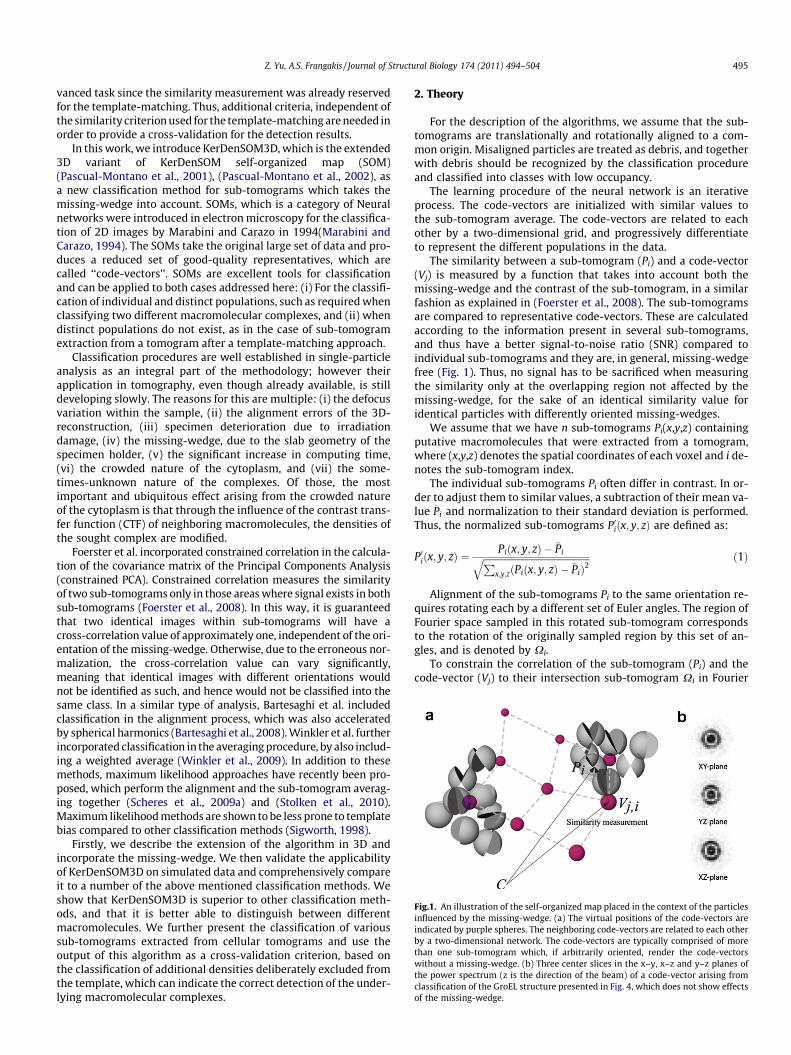
Fig.1. An illustration of the self-organized map placed in the context of the particlesinfluenced by the missing-wedge. (a) The virtual positions of the code-vectors areindicated by purple spheres. The neighboring code-vectors are related to each otherby a two-dimensional network. The code-vectors are typically comprised of morethan one sub-tomogram which, if arbitrarily oriented, render the code-vectorswithout a missing-wedge. (b) Three center slices in the x–y, x–z and y–z planes ofthe power spectrum (z is the direction of the beam) of a code-vector arising fromclassification of the GroEL structure presented in Fig. 4, which does not show effectsof the missing-wedge.

Z. Yu, A.S. Frangakis / Journal of Structural Biology 174 (2011) 494–504 495

vanced task since the similarity measurement was already reservedfor the template-matching. Thus, additional criteria, independent ofthe similarity criterion used for the template-matching are needed inorder to provide a cross-validation for the detection results.

In this work, we introduce KerDenSOM3D, which is the extended3D variant of KerDenSOM self-organized map (SOM)(Pascual-Montano et al., 2001), (Pascual-Montano et al., 2002), asa new classification method for sub-tomograms which takes themissing-wedge into account. SOMs, which is a category of Neuralnetworks were introduced in electron microscopy for the classifica-tion of 2D images by Marabini and Carazo in 1994(Marabini andCarazo, 1994). The SOMs take the original large set of data and pro-duces a reduced set of good-quality representatives, which arecalled ‘‘code-vectors’’. SOMs are excellent tools for classificationand can be applied to both cases addressed here: (i) For the classifi-cation of individual and distinct populations, such as required whenclassifying two different macromolecular complexes, and (ii) whendistinct populations do not exist, as in the case of sub-tomogramextraction from a tomogram after a template-matching approach.

Classification procedures are well established in single-particleanalysis as an integral part of the methodology; however theirapplication in tomography, even though already available, is stilldeveloping slowly. The reasons for this are multiple: (i) the defocusvariation within the sample, (ii) the alignment errors of the 3D-reconstruction, (iii) specimen deterioration due to irradiationdamage, (iv) the missing-wedge, due to the slab geometry of thespecimen holder, (v) the significant increase in computing time,(vi) the crowded nature of the cytoplasm, and (vii) the some-times-unknown nature of the complexes. Of those, the mostimportant and ubiquitous effect arising from the crowded natureof the cytoplasm is that through the influence of the contrast trans-fer function (CTF) of neighboring macromolecules, the densities ofthe sought complex are modified.

Foerster et al. incorporated constrained correlation in the calcula-tion of the covariance matrix of the Principal Components Analysis(constrained PCA). Constrained correlation measures the similarityof two sub-tomograms only in those areas where signal exists in bothsub-tomograms (Foerster et al., 2008). In this way, it is guaranteedthat two identical images within sub-tomograms will have across-correlation value of approximately one, independent of the ori-entation of the missing-wedge. Otherwise, due to the erroneous nor-malization, the cross-correlation value can vary significantly,meaning that identical images with different orientations wouldnot be identified as such, and hence would not be classified into thesame class. In a similar type of analysis, Bartesaghi et al. includedclassification in the alignment process, which was also acceleratedby spherical harmonics (Bartesaghi et al., 2008). Winkler et al. furtherincorporated classification in the averaging procedure, by also includ-ing a weighted average (Winkler et al., 2009). In addition to thesemethods, maximum likelihood approaches have recently been pro-posed, which perform the alignment and the sub-tomogram averag-ing together (Scheres et al., 2009a) and (Stolken et al., 2010).Maximum likelihood methods are shown to be less prone to templatebias compared to other classification methods (Sigworth, 1998).

Firstly, we describe the extension of the algorithm in 3D andincorporate the missing-wedge. We then validate the applicabilityof KerDenSOM3D on simulated data and comprehensively compareit to a number of the above mentioned classification methods. Weshow that KerDenSOM3D is superior to other classification meth-ods, and that it is better able to distinguish between differentmacromolecules. We further present the classification of varioussub-tomograms extracted from cellular tomograms and use theoutput of this algorithm as a cross-validation criterion, based onthe classification of additional densities deliberately excluded fromthe template, which can indicate the correct detection of the under-lying macromolecular complexes.

2. Theory

For the description of the algorithms, we assume that the sub-tomograms are translationally and rotationally aligned to a com-mon origin. Misaligned particles are treated as debris, and togetherwith debris should be recognized by the classification procedureand classified into classes with low occupancy.

The learning procedure of the neural network is an iterativeprocess. The code-vectors are initialized with similar values tothe sub-tomogram average. The code-vectors are related to eachother by a two-dimensional grid, and progressively differentiateto represent the different populations in the data.

The similarity between a sub-tomogram (Pi) and a code-vector(Vj) is measured by a function that takes into account both themissing-wedge and the contrast of the sub-tomogram, in a similarfashion as explained in (Foerster et al., 2008). The sub-tomogramsare compared to representative code-vectors. These are calculatedaccording to the information present in several sub-tomograms,and thus have a better signal-to-noise ratio (SNR) compared toindividual sub-tomograms and they are, in general, missing-wedgefree (Fig. 1). Thus, no signal has to be sacrificed when measuringthe similarity only at the overlapping region not affected by themissing-wedge, for the sake of an identical similarity value foridentical particles with differently oriented missing-wedges.

We assume that we have n sub-tomograms Pi(x,y,z) containingputative macromolecules that were extracted from a tomogram,where (x,y,z) denotes the spatial coordinates of each voxel and i de-notes the sub-tomogram index.

The individual sub-tomograms Pi often differ in contrast. In or-der to adjust them to similar values, a subtraction of their mean va-lue �Pi and normalization to their standard deviation is performed.Thus, the normalized sub-tomograms P0iðx; y; zÞ are defined as:

P0iðx; y; zÞ ¼Piðx; y; zÞ � �PiffiffiffiffiffiffiffiffiffiffiffiffiffiffiffiffiffiffiffiffiffiffiffiffiffiffiffiffiffiffiffiffiffiffiffiffiffiffiffiffiffiffiffiffiffiffiP

x;y;zðPiðx; y; zÞ � �PiÞ2q ð1Þ

Alignment of the sub-tomograms Pi to the same orientation re-quires rotating each by a different set of Euler angles. The region ofFourier space sampled in this rotated sub-tomogram correspondsto the rotation of the originally sampled region by this set of an-gles, and is denoted by Xi.

To constrain the correlation of the sub-tomogram (Pi) and thecode-vector (Vj) to their intersection sub-tomogram Xi in Fourier

496 Z. Yu, A.S. Frangakis / Journal of Structural Biology 174 (2011) 494–504

space, we need to restrict their normalization to the overlappingregion Xi, that is, the region not affected by the missing-wedgein the sub-tomogram (as the code-vector is considered missing-wedge free). We will denote by VXi

j , the code-vector that resultsfrom filtering the Fourier components not included in Xi from Vj,that is:

VXij ¼ FT�1ðFTðVjÞ �XiÞ; ð2Þ

where FT denotes the Fourier transformation and FT�1 the inverseFourier transformation.

In addition, the sub-tomograms are masked with a suitablemask M to focus the classification on certain features or reducethe effect of noise located away from the area containing signal.The sub-tomograms are normalized using the mask M in realspace:

P0iðx; y; zÞ ¼Mðx; y; zÞ � ½Piðx; y; zÞ � �Pi�ffiffiffiffiffiffiffiffiffiffiffiffiffiffiffiffiffiffiffiffiffiffiffiffiffiffiffiffiffiffiffiffiffiffiffiffiffiffiffiffiffiffiffiffiffiffiffiffiffiffiffiffiffiffiffiffiffiffiffiffiffiffiffiffiffiffiffiffiffiffiffiffiffiffiffiffiffiffiffiffiffiffiffiffiP

x0 ;y0 ;z0 ½Mðx0; y0; z0Þ � ðPiðx0; y0; z0Þ � �PiÞ�2q ð3Þ

where the mean value �Pi is constrained to M:

�Pi ¼P

x;y;zPiðx; y; zÞPx0 ;y0 ;z0Mðx0; y0; z0Þ

: ð4Þ

Using the constraint in Fourier space Xi and the mask M in realspace, the code-vectors are also normalized as:

V 0j;iðx; y; zÞ ¼Mðx; y; zÞ � ðVX

j ðx; y; zÞ � �Vj;iÞffiffiffiffiffiffiffiffiffiffiffiffiffiffiffiffiffiffiffiffiffiffiffiffiffiffiffiffiffiffiffiffiffiffiffiffiffiffiffiffiffiffiffiffiffiffiffiffiffiffiffiffiffiffiffiffiffiffiffiffiffiffiffiffiffiffiffiffiffiffiffiffiffiffiffiffiffiffiffiffiffiffiffiffiffiffiffiffiffiffiPx0 ;y0 ;z0 Mðx0; y0; z0Þ � ðVX

j ðx0; y0; z0Þ � �Vj;iÞh i2

r ð5Þ

The mean value of the code-vector �Vj;i also has to be constrainedto Xi and M:

�Vj;i ¼P

x;y;zVXij ðx; y; zÞP

x0 ;y0 ;z0 ;Mðx0; y0; z0Þ: ð6Þ

These definitions originally allowed a normalized constrainedcross-correlation between sub-tomograms to be defined;

CCCðPi; PjÞ ¼Xx;y;z

P0j;iðx; y; zÞ � P0j;iðx; y; zÞ ð7Þ

which was then used as the basis for classification by constrainedPCA, that takes the missing-wedge into account (Foerster et al.,2008). In the present work, we use the same approach as describedin (Pascual-Montano et al., 2001), but we expand it in 3D and intro-duce a missing-wedge compensation.

The expression for measuring the similarity of the sub-tomo-grams Pi to the code-vectors Vj is denoted by:

Xn

i¼1

Xc

j¼1

kPi � Vjk2uj;i; ð8Þ

where n is the number of sub-tomograms, c is the number of code-vectors, and each uj,i measures the weight of sub-tomogram Pi in thecomputation for the update of code-vector Vj (see equation (18) inPascual-Montano). Note also that computation of the uj,i requiresevaluating each term ||Pi � Vj||, where the influence of the miss-ing-wedge has to be taken into account.

The similarity of a sub-tomogram and a code-vector is thuscomputed as the Euclidean norm of the difference,

kPi � Vjk2 ¼Xx;y;z

ðPiðx; y; zÞ � Vjðx; y; zÞÞ2; ð9Þ

which in our approach is simply substituted by the Euclidean normof the difference of the normalized, constrained sub-tomogramskP0i � V 0j;ik

2 .

The KerDenSOM3D algorithm converges to a set of code-vectorsthat simultaneously maximizes two requirements: (a) their simi-larity to a set of sub-tomograms and (b) their smoothness on aset grid, which corresponds to a similarity to other neighboringcode-vectors. Both requirements are implemented in a missing-wedge compensated cost-function, similarly to the one mentionedin Eq. (14) in Pascual-Montano (Pascual-Montano et al., 2001).Note that the balance between similarity and smoothness is con-trolled by a smoothness parameter #, which appears in the numer-ical algorithm in an annealing strategy: it decreases slowly witheach step of the annealing process, from an initial value #1 to a finalvalue #0 following:

# ¼ expðlnð#1Þ � ðlnð#1Þ � lnð#0ÞÞ � iter=MaxIterÞ: ð10Þ

For each value of # the code-vectors are computed by iteratingon t the relation

V ðtþ1Þj ¼

Pni¼1uðtÞj;i Pi þ #V ðtÞjPn

i¼1uðtÞj;i þ #; uðtÞj;i

¼ uðtÞj;i kPi0 � V ðtÞj0kgi0 ;j0 ; fV

ðtÞj0

n oj0; #

� �; ð11Þ

until convergence is achieved (V ðtÞj is the average of the code-vectors that are neighbors of V ðtÞj on the grid, excluding V ðtÞj itselffrom the average).

The smoothness parameter # and the grid size are practicallythe only parameters relevant for a classification. The followingempirical values are suggested for the classification of datasets:#1 ¼ 30 n

c, #0 ¼ 3 nc, the number of annealing steps set to 50and a

grid size of 5 � 5 or larger. The smoothness parameter dependson the number of sub-tomograms n and the size of the grid c.

The formula for the smoothness parameters # can be derived byassuming that the contribution of all the sub-tomograms to all

code-vectors is the same, thus: uji ¼ 1c ;8j; i and V ðtþ1Þ

j ¼nc�Xþ#V ðtÞ

jncþ#

,

where V ðtþ1Þj is the jth code-vector in (t + 1)th step, n is the number

of the sub-tomograms, and all code-vectors are initially identical.For datasets with same image size, recorded at similar conditionsand similar SNR, the ratio n=c

#has to be set to the empirical values

suggested above in order to obtain a good performance. Thus, anexhaustive search of parameters can be avoided, which is of greatadvantage to any user, since a scan of these parameters may oftenbe the most burdensome and time-consuming part of the classifi-cation procedure.

3. Materials and methods

The algorithm was implemented in MATLAB (The MathWorks,Inc.) and C/C++ for massive parallel processing. The algorithmsare available upon request, and the source code can be downloadedat http://www.biophys.uni-frankfurt.de/frangakis/.

3.1. Acquisition conditions

The tilt-series were recorded on a 300 kV, Tecnai G2 Polara FEGand a CM300 transmission electron microscope (FEI, Eindhoven,The Netherlands) equipped with a Gatan post-column GIF 2002 en-ergy filter (Pleasanton, CA). Tomographic single-tilt-series were ac-quired using either the TOM Toolbox or the UCSF software packagewith zero-loss filtering (slit-width of 30 eV) (Nickell et al., 2005;Zheng et al., 2004). The individual projection images recorded withthe microscope were interactively aligned with respect to a com-mon origin using 10 nm colloidal gold particles distributed in thesamples as fiducial markers. Reconstructions were performed

Z. Yu, A.S. Frangakis / Journal of Structural Biology 174 (2011) 494–504 497

using weighted backprojection. Visualization was performed withthe Amira package (Pruggnaller et al., 2008).

3.2. Simulated data

The simulated data used in Foerster et al. was also used here inorder to allow for a direct comparison of the performance of thealgorithms. A detailed description for generating the data is givenin Foerster et al. chapter 3.2 (Foerster et al., 2008). The goal of thesimulation was to produce realistic tomograms. In brief: The den-sity of the macromolecule was rotated around a single axis, pro-jected onto a plane and superimposed with Gaussian noise. Onthe resulting 2D-image, the CTF was applied. The CTF wascomposed of two terms: (i) the idealized CTF assuming pure phasecontrast at a particular defocus and (ii) a modulation-transfer func-tion (MTF) that describes the imaging properties of the CCD-cam-era. On the resulting image, noise was added representingbackground noise due to non-elastic scattering events and thereadout noise of the CCD-camera. The resulting projections werethen merged into the sub-tomogram using weighted backprojec-tion. The main parameters varying in the simulation are the half-opening angle W of the missing-wedge (as the half angle of theopening of the missing-wedge, i.e. a half-opening angle W of 20degrees would correspond to a tilt-series from -70 to + 70 degrees)and the SNR.

3.3. Acquisition of the in vitro GroEL and GroEL/GroES tomograms

For comparison purposes, the same sub-tomograms were usedas in Foerster et al. and Scheres et al. In brief: 1 lM GroEL14 wasincubated with and without 5 lM GroES7 in a buffer containing12.5 mM Hepes (pH 7.5), 5 mM KCl, 5 mM MgCl2, 1 mM DTT,and 5 mM ADP for 15 min at 30 �C. Protein solutions (3.5 ll) weremixed with 0.5 ll of a 10 nm BSA-colloidal gold suspension, ap-plied to 300 mesh grids coated with Lacey carbon films (Plano,Wetzlar, Germany) and vitrified by plunge-freezing. Single-axistilt-series were collected covering an angular range from �65� to+65� with 2� or 2.5� angular increment. Images were recorded ona 2 k � 2k pixel CCD camera at a defocus level of �4 lm to mimicthe real experimental conditions of cellular tomography. The pixelsize at the specimen level was 0.6 nm.

3.4. Cryo-electron tomography of Mycoplasma pneumonia andSpiroplasma melliferum

For cellular tomography, we analyzed tomograms used in previ-ous studies (Kuerner et al., 2005; Seybert et al., 2006). Detaileddescription of the cultivation of the strains can be found in the ref-erences. The tilt-series were acquired between �66� and +66� forM. pneumonia and �60� to +60� for S. melliferum with a tilt incre-ment of 1.5�. The images were recorded at defocus between �5and �10 lm and a pixel size on the CCD camera of 0.6 nm or0.68 nm at the specimen plane.

4. Results

4.1. Simulated data: ‘‘Open’’ and ‘‘Closed’’ thermosomes

In order to assess the quality of the classification with KerDen-SOM3D, we applied it to the same simulated tomographic data asin Foerster et al. (Foerster et al., 2008), where the constrained cor-relation was tested. This provides the possibility for direct compar-ison of the two techniques. The simulated object used was thearchaeal chaperonin thermosome in its open and closed conforma-tions. For the closed conformation, the pdb coordinates from the

X-ray structure were used (1A6D)(Ditzel et al., 1998), and for theopen conformation, a structure derived from a molecular model fit-ted to a single-particle EM density map was used (Nitsch et al.,1998).

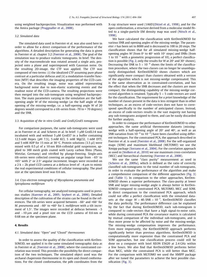
We have calculated the classification with KerDenSOM3D forvarious SNR and opening angles of the missing-wedge. The param-eter # has been set to 8000 and is decreased to 100 in 20 steps. Theclassification shows that for all simulated missing-wedge half-opening angles W (from 0� to 40� with 10� steps) and SNRs (from1 to 10�3 with a geometric progression of 10), a perfect classifica-tion is possible (Fig. 2, only the results for W at 20� and 30� shown).Decreasing the SNR to 5 � 10�4 shows the limits of the classifica-tion procedure, where the two classes can no longer be unambigu-ously distinguished. KerDenSOM3D shows clusters which aresignificantly more compact than clusters obtained with a versionof the algorithm which is not missing-wedge compensated. Thisis the same observation as in constrained-correlation, and hasthe effect that when the SNR decreases and the clusters are morecompact, the distinguishing capability of the missing-wedge cor-rected algorithm is retained. Typically 5 � 5 code-vectors are usedfor the classification. The requirement for a priori knowledge of thenumber of classes present in the data is less stringent than in othertechniques, as an excess of code-vectors does not have to corre-spond specifically to the number of anticipated classes. Instead,an excess of code-vectors results in the vast majority not havingany sub-tomograms assigned to them, and can be easily discardedfor further analysis.

In order to compare the performance of KerDenSOM3D to otherapproaches, the same artificial thermosome datasets (missing-wedge with a half-opening angle of 20� and 40�, as well as anSNR variation from 10�4 to 10�2) have been classified using differ-ent techniques. For the constrained PCA, the approach described inFoerster et al. is used (Foerster et al., 2008). For the self-organizedmaps (SOM) and maximum likelihood (MLTOMO) we use theXmipp package (Sorzano et al., 2004). For the correlation approachas used in (Stolken et al., 2010) we use maximum cross-correlation(MCC) and hierarchical clustering (Foerster et al., 2008).

We use the same ’’class purity’’ measurement as used in(Scheres et al., 2009a), which is defined as the ratio of correctlyclassified sub-tomograms to the total number of sub-tomograms,in order to evaluate the performance of the algorithm and makea comprehensive comparison of the different approaches (Fig. 3)and (Table 1). In comparison to the other approaches, KerDen-SOM3D shows a superior performance. The class-purity at lowerSNR and larger missing-wedge angle is always better in KerDen-SOM3D compared to constrained PCA, MLTOMO, MCC and SOM.In direct comparison to the constrained PCA approach, whichcould not offer a perfect classification with the simulated data-sets at the stage W ¼ 40; SNR ¼ 10�3, KerDenSOM3D classifiesthe data perfectly. The performance difference can be explainedby the fact that during KerDenSOM3D, each sub-tomogram iscompared to code-vectors that have a high signal-to-noise ratio,while during constrained PCA the covariance matrix is calculatedby mutual comparison of the individual sub-tomograms, and isthus more prone to be affected by noise and the missing-wedge.The missing-wedge compensation improves the performance.Even more importantly, the KerDenSOM3D approach performssignificantly better than previous algorithms. KerDenSOM3D iscomputationally more expensive than the constrained PCA andSOM approaches, but one classification process could still bedone on a computer with Intel XEON E5620 at 2.4 GHz withina few hours. We also find that KerDenSOM3D performs betterthan MCC, while the constrained PCA is still better than MCC.For the comparison with MLTOMO we used the XMIPP packageafter we tuned the parameters to achieve the best possible clas-sification (Fig. 3).

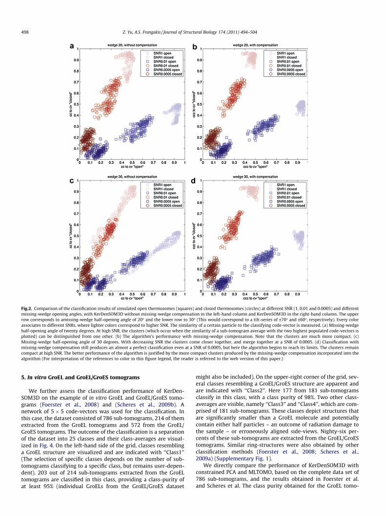
Fig.2. Comparison of the classification results of simulated open thermosomes (squares) and closed thermosomes (circles) at different SNR (1, 0.01 and 0.0005) and differentmissing-wedge opening angles, with KerDenSOM3D without missing-wedge compensation in the left-hand column and KerDenSOM3D in the right-hand column. The upperrow corresponds to amissing-wedge half-opening angle of 20� and the lower row to 30� (This would correspond to a tilt-series of ±70� and ±60�, respectively). Every colorassociates to different SNRs, where lighter colors correspond to higher SNR. The similarity of a certain particle to the classifying code-vector is measured. (a) Missing-wedgehalf-opening angle of twenty degrees. At high SNR, the clusters (which occur when the similarity of a sub-tomogram average with the two highest populated code-vectors isplotted) can be distinguished from one other. (b) The algorithm’s performance with missing-wedge compensation. Note that the clusters are much more compact. (c)Missing-wedge half-opening angle of 30 degrees. With decreasing SNR the clusters come closer together, and merge together at a SNR of 0.0005. (d) Classification withmissing-wedge compensation still produces an almost a perfect classification even at a SNR of 0.0005, but here the algorithm begins to reach its limits. The clusters remaincompact at high SNR. The better performance of the algorithm is justified by the more compact clusters produced by the missing-wedge compensation incorporated into thealgorithm (For interpretation of the references to color in this figure legend, the reader is referred to the web version of this paper.)

498 Z. Yu, A.S. Frangakis / Journal of Structural Biology 174 (2011) 494–504

5. In vitro GroEL and GroEL/GroES tomograms

We further assess the classification performance of KerDen-SOM3D on the example of in vitro GroEL and GroEL/GroES tomo-grams (Foerster et al., 2008) and (Scheres et al., 2009b). Anetwork of 5 � 5 code-vectors was used for the classification. Inthis case, the dataset consisted of 786 sub-tomograms, 214 of themextracted from the GroEL tomograms and 572 from the GroEL/GroES tomograms. The outcome of the classification is a separationof the dataset into 25 classes and their class-averages are visual-ized in Fig. 4. On the left-hand side of the grid, classes resemblinga GroEL structure are visualized and are indicated with ‘‘Class1’’(The selection of specific classes depends on the number of sub-tomograms classifying to a specific class, but remains user-depen-dent). 203 out of 214 sub-tomograms extracted from the GroELtomograms are classified in this class, providing a class-purity ofat least 95% (individual GroELs from the GroEL/GroES dataset

might also be included). On the upper-right corner of the grid, sev-eral classes resembling a GroEL/GroES structure are apparent andare indicated with ‘‘Class2’’. Here 177 from 181 sub-tomogramsclassify in this class, with a class purity of 98%. Two other class-averages are visible, namely ‘‘Class3’’ and ‘‘Class4’’, which are com-prised of 181 sub-tomograms. These classes depict structures thatare significantly smaller than a GroEL molecule and potentiallycontain either half particles – an outcome of radiation damage tothe sample – or erroneously aligned side-views. Nighty-six per-cents of these sub-tomograms are extracted from the GroEL/GroEStomograms. Similar ring-structures were also obtained by otherclassification methods (Foerster et al., 2008; Scheres et al.,2009a) (Supplementary Fig. 1).

We directly compare the performance of KerDenSOM3D withconstrained PCA and MLTOMO, based on the complete data set of786 sub-tomograms, and the results obtained in Foerster et al.and Scheres et al. The class purity obtained for the GroEL tomo-

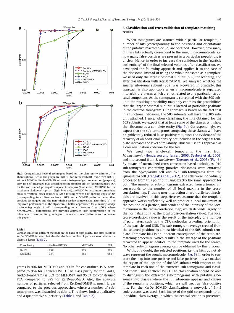
Fig.3. Comparisonof several techniques based on the class-purity criterion. Theabbreviations used in the graph are: KDS3D for KerdenSOM3D (red circle), KDS3Dwithout MWC for KerdenSOM3D without missing-wedge compensation (purple x),SOM for Self-organized map according to the simplest edition (green triangle), PCAfor the constrained principal components analysis (blue cross), MLTOMO for themaximum likelihood approach (light blue dot), and MCC for maximum constrainedcross-correlation (black square). (a) At a missing-wedge half-opening angle of 20�(corresponding to a tilt-series from ±70�), KerdenSOM3D performs better thanprevious techniques and the non-missing-wedge compensated algorithm. (b) Theimproved performance of the algorithm is better appreciated for a missing-wedgehalf-opening angle of 40� (corresponding to a tilt-series from ±50�), whereKerDenSOM3D outperforms any previous approach (For interpretation of thereferences to color in this figure legend, the reader is referred to the web version ofthis paper.)

Table 1Comparison of the different methods on the basis of class-purity. The class-purity inKerDenSOM3D is better, but also the absolute number of particles associated to theclasses is larger (Table 2).

Class Purity KerDenSOM3D MLTOMO PCA

GroEL 95% 90% 90%GroEL/ES 98% 86% 95%

Z. Yu, A.S. Frangakis / Journal of Structural Biology 174 (2011) 494–504 499

grams is 90% for MLTOMO and 90.5% for constrained PCA, com-pared to 95% for KerDenSOM3D. The class purity for the GroEL/GroES tomograms is 86% for MLTOMO and 95.5% for constrainedPCA, compared to 98% for KerDenSOM3D. Also, the absolutenumber of particles selected from KerDenSOM3D is much largercompared to the previous approaches, where a number of sub-tomograms was discarded as debris. This shows both a qualitativeand a quantitative superiority (Table 1 and Table 2).

6. Classification and cross-validation of template-matchingresults

When tomograms are scanned with a particular template, anumber of hits (corresponding to the positions and orientationsof the putative macromolecule) are obtained. However, how manyof these hits actually correspond to the sought macromolecule, i.e.how many false-positives are present in a particular population, isunclear. Hence, in order to increase the confidence in the ‘‘particleauthenticity’’ of the final selected volumes after classification, wedeveloped the following approach and applied it to the case ofthe ribosome. Instead of using the whole ribosome as a template,we used only the large ribosomal subunit (50S) for scanning, andafter classification with KerDenSOM3D we analysed whether thesmaller ribosomal subunit (30S) was recovered. In principle, thisapproach is also applicable when a macromolecule is separatedinto arbitrary pieces which are not related to any particular struc-tural component. As the tomogram is correlated with the 50S sub-unit, the resulting probability map only contains the probabilitiesthat the large ribosomal subunit is located at particular positionsin the electron tomogram. Our approach is based on the fact thatin a functional ribosome, the 50S subunits will have the 30S sub-unit attached. Hence, when classifying the hits obtained for the50S subunit, we expect that at least some of the classes will showthe ribosome as a complete entity (Fig. 5a). Correspondingly, weexpect that the sub-tomograms composing those classes will havea significantly reduced false-positive rate, since the evidence of therecovery of an additional density not included in the original tem-plate increases the level of reliability. Thus we use this approach asa cross-validation criterion for the hits.

We used two whole-cell tomograms, the first fromM. pneumonia (Henderson and Jensen, 2006; Seybert et al., 2006)and the second from S. melliferum (Kuerner et al., 2005) (Fig. 6).By means of normalized cross-correlation-based techniques, 919sub-tomograms containing putative ribosomes were extractedfrom the Mycoplasma cell and 876 sub-tomograms from theSpiroplasma cell (Frangakis et al., 2002). The cells were individuallyprocessed from this point but using exactly the same approach forboth. The number of sub-tomograms extracted from a tomogramcorresponds to the number of all local maxima in the cross-correlation map. Thus, no user-interaction or arbitrarily set thresh-olds are involved in this step. Here we assume that the templateapproach works sufficiently well to produce a local maximum atthe position of a particle, independent of the intensity of the localmaximum in the cross-correlation map, which depends largely onthe normalization (i.e. the local cross-correlation value). The localcross-correlation value is the result of the interplay of a numberof parameters such as the CTF, molecular crowding, orientationof the particle, and SNR. The sub-tomogram average created fromthe selected positions is almost identical to the 50S subunit tem-plate. Template bias is an inherent consequence of the template-matching procedure, which results in the average of the positionsrecovered to appear identical to the template used for the search.No other sub-tomogram average can be obtained by this process.

Without a doubt, the selected positions, i.e. the hits, do not al-ways represent the sought macromolecule (Fig. 6). In order to sep-arate the map into true-positive and false-positive hits, we maskedthe region of the location of the 30S subunit with respect to thetemplate in each one of the extracted sub-tomograms and classi-fied them using KerDenSOM3D. The classification should be ableto distinguish the extracted sub-tomograms with putative ribo-somes into classes where the full ribosome appears and classesof the remaining positions, which we will treat as false-positivehits. For the KerDenSOM3D classification, a network of 5 � 5code-vectors was used. Each image of the grid corresponds to anindividual class-average in which the central section is presented.

Fig.4. Classification of the GroEL and GroEL/GroES in vitro datasets. (a) Visualization of the central slice of the class-averages in a 5 � 5 self-organized map. In the inset of eachclass-average, the number of sub-tomograms classifying to each code-vector is indicated. In blue, the total number of sub-tomograms in the class; in red, sub-tomogramsoriginating from the GroEL dataset; in yellow, sub-tomograms originating from the GroEL/GroES dataset. Four classes can be distinguished, namely, Class 1 which representsGroEL (left part of the map); Class 2 which represents GroEL/GroES complexes (upper right corner of the map); and two classes with half particles (Classes 3 and 4). The vastmajority of the half particles originate from the GroEL/GroES dataset. The upper-right class contains GroEL/GroES-similar particles and the lower-right class contains GroEL-similar particles. The scale bar in the lower-right corner applies to all images and is 10 nm in length. (b) x–y section and (c) y–z the sections of the averages of the particlesclassifying to a GroEL-similar class.7-fold symmetry can be observed. 203 out of 214 sub-tomograms extracted from the GroEL tomograms contribute to this average. (d) x–ysection and (e) y–z section of the average of the particles classifying to a GroEL/GroES-similar class. 177 out of 181 particles classified to this class originate from the GroEL/GroES tomograms, presenting a class purity of 98%. The scale bar is 10 nm (For interpretation of the references to color in this figure legend, the reader is referred to the webversion of this paper.)

Table 2Comparison of the different methods on the basis of the total number of sub-tomograms associated to each class. From the complete set of 786 sub-tomograms, KerDenSOM3Dassociated 424 sub-tomograms to GroEL and 181 to GroEL/ES. The remaining particles are associated to other classes. In contrast, PCA associated 377 sub-tomograms to GroELand 222 to GroEL/ES. The class-purity in KerDenSOM3D is better, but also the absolute number of particles associated to the classes is larger. The absolute number of particlesclassified to the class GroEL/ES with MLTOMO is unknown (Scheres et al., 2009a) and is marked with question mark.

KerDenSOM3D MLTOMO PCA

Total GroEL GroEL/ES Total GroEL GroEL/ES Total GroEL GroEL/ES

GroEL Class 424 203 221 ? 193 ? 377 182 195GroEL/ES Class 181 4 177 150 21 129 222 10 212

500 Z. Yu, A.S. Frangakis / Journal of Structural Biology 174 (2011) 494–504

In the upper-right part of the map (second row, last column), adensity next to the ribosome is shown, which resembles the den-sity of the 30S subunit well (Fig. 5a and b).

Unfortunately, classifying density within a mask at a specificposition also introduces a bias. As a thought-experiment, we notethat the sub-tomograms which are used for the averaging are clas-sified according to the high intensity values within the mask. Con-sequently, the resulting class-averages look similar to the totalaverage of all the sub-tomograms (the 50S subunit), with an in-creased density at the location of the mask which was used forthe classification. In order to increase the confidence that we re-cover the 30S subunit density in its true position, and that no pos-sible bias is introduced by either the mask or the shape of themask, we performed an additional cross-validation experiment.We exhaustively scanned the surrounding of the 50S subunit withvarious transformed 30S subunit masks, and verified that the prop-erties are different, when the mask is at the true 30S subunit posi-tion compared to any other position.

Let us call M the mask that tightly covers the true position of the30S subunit. We define a set of affine transformations of M thatproduce a set of masks that cover the neighborhood of the 50S sub-unit. Each transformed mask, Md ¼ RdðMÞ, is called a decoy (Fig. 5c).Here, each Rd represents the action of a rotation followed by atranslation, and d ranges from 1 to 104, where decoy 104 is re-served for the true position of the 30S subunit. The set of transfor-

mations was chosen arbitrarily, but it was ascertained that allvoxels in the immediate surroundings of the 50S subunit were lo-cated within some decoys (Fig. 5c).

For each decoy Md, we classify the entire set of sub-tomogramsfPigi2I using only the voxels included in the decoy. The results ofeach classification can be represented by a partition of the set Iof sub-tomogram indexes into C subsets:

I ¼[Cc¼1

Id;c: ð12Þ

Here, Id;c represents the indices of the sub-tomograms that wereassigned to a class c by the classifying algorithm, where c is thenumber of classes generated. The sub-tomogram average of eachclass is denoted by Xd;c with the definition:

Pd;cðx; y; zÞ ¼P

i2Id;c Piðx; y; zÞ#Id;c

; ð13Þ

where # expresses the number of elements in a set. Now, we com-pute in each classification the class number of the average whichbest resembles the template of the 30S subunit (transformed asthe corresponding decoy). This resemblance, denoted by sd is mea-sured by cross-correlation, only taking into consideration the voxelsincluded in Md. The resulting class number is denoted by cd.

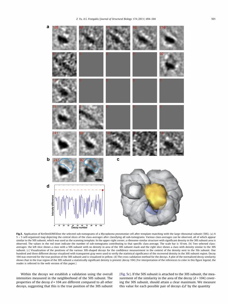
Fig.5. Application of KerDenSOM3Don the selected sub-tomograms of a Mycoplasma pneumoniae cell after template-matching with the large ribosomal subunit (50S). (a) A5 � 5 self-organized map depicting the central slices of the class-averages after classifying all sub-tomograms. Various class-averages can be observed, all of which appearsimilar to the 50S subunit, which was used as the scanning template. In the upper-right corner, a ribosome-similar structure with significant density in the 30S subunit area isobserved. The values in the red inset indicate the number of sub-tomograms contributing to that specific class-average. The scale bar is 10 nm. (b) Two selected class-averages: the left slice shows a class with a 50S subunit with no density in area of the 30S subunit mask and the right slice shows a class with density similar to the 30Ssubunit. (c) Visualization of the positions of the various 30S-shaped decoys for the confidence measurement in the context of the density next to the 50s subunit. Onehundred and three different decoys visualized with transparent gray were used to verify the statistical significance of the recovered density in the 30S subunit region. Decoy104 was reserved for the true position of the 30S subunit and is visualized in yellow. (d) The cross-validation method for the decoys. A plot of the normalized decoy similarityshows that in the true region of the 30S subunit a statistically significant density is present (decoy 104) (For interpretation of the references to color in this figure legend, thereader is referred to the web version of this paper.)

Z. Yu, A.S. Frangakis / Journal of Structural Biology 174 (2011) 494–504 501

Within the decoys we establish a validation using the overallintensities measured in the neighborhood of the 50S subunit. Theproperties of the decoy d = 104 are different compared to all otherdecoys, suggesting that this is the true position of the 30S subunit

(Fig. 5c). If the 50S subunit is attached to the 30S subunit, the mea-surement of the similarity in the area of the decoy (d = 104) cover-ing the 30S subunit, should attain a clear maximum. We measurethis value for each possible pair of decoys d,d’ by the quantity

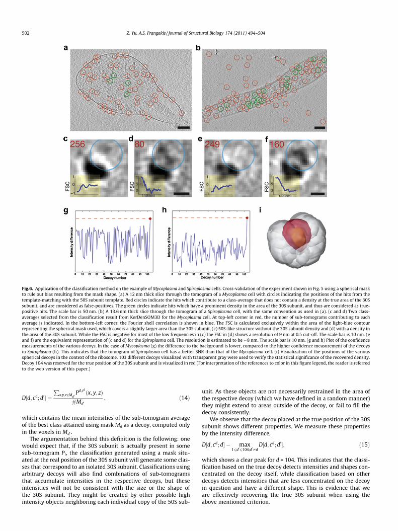
Fig.6. Application of the classification method on the example of Mycoplasma and Spiroplasma cells. Cross-validation of the experiment shown in Fig. 5 using a spherical maskto rule out bias resulting from the mask shape. (a) A 12 nm thick slice through the tomogram of a Mycoplasma cell with circles indicating the positions of the hits from thetemplate-matching with the 50S subunit template. Red circles indicate the hits which contribute to a class-average that does not contain a density at the true area of the 30Ssubunit, and are considered as false-positives. The green circles indicate hits which have a prominent density in the area of the 30S subunit, and thus are considered as true-positive hits. The scale bar is 50 nm. (b) A 13.6 nm thick slice through the tomogram of a Spiroplasma cell, with the same convention as used in (a). (c and d) Two class-averages selected from the classification result from KerDenSOM3D for the Mycoplasma cell. At top-left corner in red, the number of sub-tomograms contributing to eachaverage is indicated. In the bottom-left corner, the Fourier shell correlation is shown in blue. The FSC is calculated exclusively within the area of the light-blue contourrepresenting the spherical mask used, which covers a slightly larger area than the 30S subunit. (c) 50S-like structure without the 30S subunit density and (d) with a density inthe area of the 30S subunit. While the FSC is negative for most of the low frequencies in (c) the FSC in (d) shows a resolution of 9 nm at 0.5 cut-off. The scale bar is 10 nm. (eand f) are the equivalent representation of (c and d) for the Spiroplasma cell. The resolution is estimated to be �8 nm. The scale bar is 10 nm. (g and h) Plot of the confidencemeasurements of the various decoys. In the case of Mycoplasma (g) the difference to the background is lower, compared to the higher confidence measurement of the decoysin Spiroplasma (h). This indicates that the tomogram of Spiroplasma cell has a better SNR than that of the Mycoplasma cell. (i) Visualization of the positions of the variousspherical decoys in the context of the ribosome. 103 different decoys visualized with transparent gray were used to verify the statistical significance of the recovered density.Decoy 104 was reserved for the true position of the 30S subunit and is visualized in red (For interpretation of the references to color in this figure legend, the reader is referredto the web version of this paper.)

502 Z. Yu, A.S. Frangakis / Journal of Structural Biology 174 (2011) 494–504

D½d; cd; d0� ¼P

x;y;z2Md0Pd;cd ðx; y; zÞ

#Md0; ð14Þ

which contains the mean intensities of the sub-tomogram averageof the best class attained using mask Md as a decoy, computed onlyin the voxels in Md0 .

The argumentation behind this definition is the following: onewould expect that, if the 30S subunit is actually present in somesub-tomogram Pi, the classification generated using a mask situ-ated at the real position of the 30S subunit will generate some clas-ses that correspond to an isolated 30S subunit. Classifications usingarbitrary decoys will also find combinations of sub-tomogramsthat accumulate intensities in the respective decoys, but theseintensities will not be consistent with the size or the shape ofthe 30S subunit. They might be created by other possible highintensity objects neighboring each individual copy of the 50S sub-

unit. As these objects are not necessarily restrained in the area ofthe respective decoy (which we have defined in a random manner)they might extend to areas outside of the decoy, or fail to fill thedecoy consistently.

We observe that the decoy placed at the true position of the 30Ssubunit shows different properties. We measure these propertiesby the intensity difference,

D½d; cd; d� � max16d06104;d0–d

D½d; cd; d0�; ð15Þ

which shows a clear peak for d = 104. This indicates that the classi-fication based on the true decoy detects intensities and shapes con-centrated on the decoy itself, while classification based on otherdecoys detects intensities that are less concentrated on the decoyin question and have a different shape. This is evidence that weare effectively recovering the true 30S subunit when using theabove mentioned criterion.

Z. Yu, A.S. Frangakis / Journal of Structural Biology 174 (2011) 494–504 503

In order to also verify that the density which appears next to the50S subunit is not dependant on the shape of the mask, we rerunthe process described above with featureless spherical decoys.For sub-tomograms extracted from both cells, a density resemblingthe shape of the 30S subunit appears again at the proper positionwith respect to the 50S subunit. Using the Fourier shell correlation(FSC),the resolution of these sub-tomogram averages was esti-mated to be 9 and 8 nm for the Mycoplasma and Spiroplasma data-sets respectively (Fig. 6d and f). The FSC is calculated only withinthe recovered density, and not for the complete structure, in orderto avoid any improvement originating from template bias. Whenthe intensity difference values within the decoys are measured,the decoy at the true position shows a significant higher value thenthe surrounding (Fig. 6g and h).

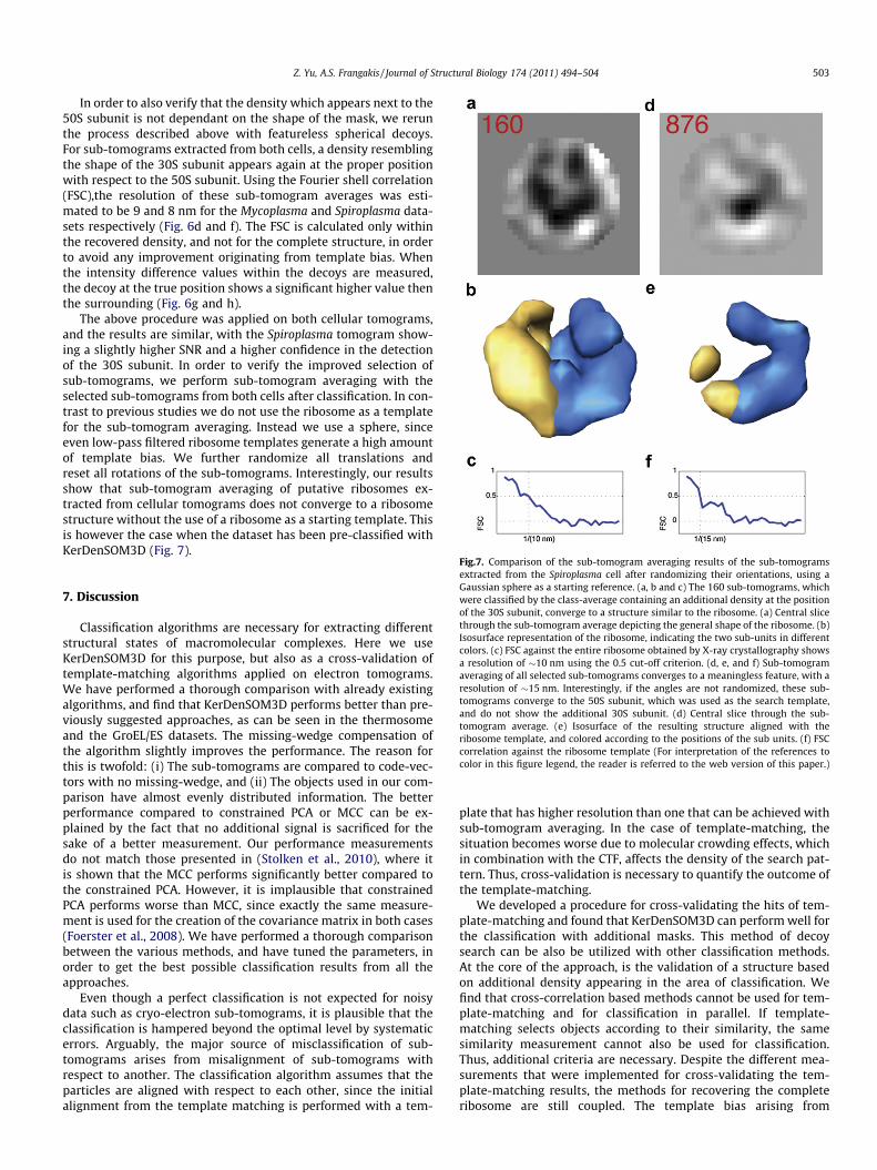
The above procedure was applied on both cellular tomograms,and the results are similar, with the Spiroplasma tomogram show-ing a slightly higher SNR and a higher confidence in the detectionof the 30S subunit. In order to verify the improved selection ofsub-tomograms, we perform sub-tomogram averaging with theselected sub-tomograms from both cells after classification. In con-trast to previous studies we do not use the ribosome as a templatefor the sub-tomogram averaging. Instead we use a sphere, sinceeven low-pass filtered ribosome templates generate a high amountof template bias. We further randomize all translations andreset all rotations of the sub-tomograms. Interestingly, our resultsshow that sub-tomogram averaging of putative ribosomes ex-tracted from cellular tomograms does not converge to a ribosomestructure without the use of a ribosome as a starting template. Thisis however the case when the dataset has been pre-classified withKerDenSOM3D (Fig. 7).

Fig.7. Comparison of the sub-tomogram averaging results of the sub-tomogramsextracted from the Spiroplasma cell after randomizing their orientations, using aGaussian sphere as a starting reference. (a, b and c) The 160 sub-tomograms, whichwere classified by the class-average containing an additional density at the positionof the 30S subunit, converge to a structure similar to the ribosome. (a) Central slicethrough the sub-tomogram average depicting the general shape of the ribosome. (b)Isosurface representation of the ribosome, indicating the two sub-units in differentcolors. (c) FSC against the entire ribosome obtained by X-ray crystallography showsa resolution of �10 nm using the 0.5 cut-off criterion. (d, e, and f) Sub-tomogramaveraging of all selected sub-tomograms converges to a meaningless feature, with aresolution of �15 nm. Interestingly, if the angles are not randomized, these sub-tomograms converge to the 50S subunit, which was used as the search template,and do not show the additional 30S subunit. (d) Central slice through the sub-tomogram average. (e) Isosurface of the resulting structure aligned with theribosome template, and colored according to the positions of the sub units. (f) FSCcorrelation against the ribosome template (For interpretation of the references tocolor in this figure legend, the reader is referred to the web version of this paper.)

7. Discussion

Classification algorithms are necessary for extracting differentstructural states of macromolecular complexes. Here we useKerDenSOM3D for this purpose, but also as a cross-validation oftemplate-matching algorithms applied on electron tomograms.We have performed a thorough comparison with already existingalgorithms, and find that KerDenSOM3D performs better than pre-viously suggested approaches, as can be seen in the thermosomeand the GroEL/ES datasets. The missing-wedge compensation ofthe algorithm slightly improves the performance. The reason forthis is twofold: (i) The sub-tomograms are compared to code-vec-tors with no missing-wedge, and (ii) The objects used in our com-parison have almost evenly distributed information. The betterperformance compared to constrained PCA or MCC can be ex-plained by the fact that no additional signal is sacrificed for thesake of a better measurement. Our performance measurementsdo not match those presented in (Stolken et al., 2010), where itis shown that the MCC performs significantly better compared tothe constrained PCA. However, it is implausible that constrainedPCA performs worse than MCC, since exactly the same measure-ment is used for the creation of the covariance matrix in both cases(Foerster et al., 2008). We have performed a thorough comparisonbetween the various methods, and have tuned the parameters, inorder to get the best possible classification results from all theapproaches.

Even though a perfect classification is not expected for noisydata such as cryo-electron sub-tomograms, it is plausible that theclassification is hampered beyond the optimal level by systematicerrors. Arguably, the major source of misclassification of sub-tomograms arises from misalignment of sub-tomograms withrespect to another. The classification algorithm assumes that theparticles are aligned with respect to each other, since the initialalignment from the template matching is performed with a tem-

plate that has higher resolution than one that can be achieved withsub-tomogram averaging. In the case of template-matching, thesituation becomes worse due to molecular crowding effects, whichin combination with the CTF, affects the density of the search pat-tern. Thus, cross-validation is necessary to quantify the outcome ofthe template-matching.

We developed a procedure for cross-validating the hits of tem-plate-matching and found that KerDenSOM3D can perform well forthe classification with additional masks. This method of decoysearch can be also be utilized with other classification methods.At the core of the approach, is the validation of a structure basedon additional density appearing in the area of classification. Wefind that cross-correlation based methods cannot be used for tem-plate-matching and for classification in parallel. If template-matching selects objects according to their similarity, the samesimilarity measurement cannot also be used for classification.Thus, additional criteria are necessary. Despite the different mea-surements that were implemented for cross-validating the tem-plate-matching results, the methods for recovering the completeribosome are still coupled. The template bias arising from

504 Z. Yu, A.S. Frangakis / Journal of Structural Biology 174 (2011) 494–504

template-matching remains contained within each sub-tomogram.The resulting ribosome structure has a prominent white stripebetween the 50S subunit and 30S subunit (Fig. 7), which indicatesthat some false-positives still exist despite the fact that the classi-fication successfully removed a significant number. This is notunusual, and the effect will likely never be completely eliminated,and unfortunately the number of false positives cannot be esti-mated or even eliminated. Even in single-particle analysis wherethe signal is stronger and the search area more restricted, a tem-plate bias is still present (Shaikh et al., 2003). However, when someof the signal is recovered, it is an indication that the algorithm per-forms well. This is the first approach for improving the confidenceof the detection results, and we combined three criteria: (i) classi-fying density within a mask that covers an area of the sought mac-romolecule which was not used for template matching; (ii) theintroduction of decoy masks around the true area of density in or-der to verify the statistical significance of the finding, and (iii) theFSC between the recovered density and the true missing part of thesought macromolecule. Nevertheless, continued algorithmic devel-opment is required in order to increase the confidence. Increasedcomputational power will allow for statistical improvement ofthe results and the class purity.

Acknowledgments

Daniel Castano and Sabine Pruggnaller for the first implementa-tion of the algorithm, Wolfgang Baumeister for the Spiroplasmamelliferum data, and the European Research Council for the ERCstarting grant to AF.

Appendix A. Supplementary data

Supplementary data associated with this article can be found, inthe online version, at doi:10.1016/j.jsb.2011.02.009.

References

Al-Amoudi, A., Diez, D.C., Betts, M.J., Frangakis, A.S., 2007. The moleculararchitecture of cadherins in native epidermal desmosomes. Nature 450, 832–837.

Bartesaghi, A., Sprechmann, P., Liu, J., Randall, G., Sapiro, G., Subramaniam, S., 2008.Classification and 3D averaging with missing wedge correction in biologicalelectron tomography. J. Struct. Biol. 162, 436–450.

Beck, M., Forster, F., Ecke, M., Plitzko, J.M., Melchior, F., Gerisch, G., Baumeister, W.,Medalia, O., 2004. Nuclear pore complex structure and dynamics revealed bycryoelectron tomography. Science 306, 1387–1390.

Brandt, F., Etchells, S.A., Ortiz, J.O., Elcock, A.H., Hartl, F.U., Baumeister, W., 2009. Thenative 3D organization of bacterial polysomes. Cell 136, 261–271.

Briggs, J.A., Riches, J.D., Glass, B., Bartonova, V., Zanetti, G., Krausslich, H.G., 2009.Structure and assembly of immature HIV. Proc. Natl. Acad. Sci. USA 106, 11090–11095.

Ditzel, L., Lowe, J., Stock, D., Stetter, K.O., Huber, H., Huber, R., Steinbacher, S., 1998.Crystal structure of the thermosome, the archaeal chaperonin and homolog ofCCT. Cell 93, 125–138.

Foerster, F., Pruggnaller, S., Seybert, A., Frangakis, A.S., 2008. Classification of cryo-electron sub-tomograms using constrained correlation. J. Struct. Biol. 161, 276–286.

Frangakis, A.S., Bohm, J., Forster, F., Nickell, S., Nicastro, D., Typke, D., Hegerl, R.,Baumeister, W., 2002. Identification of macromolecular complexes incryoelectron tomograms of phantom cells. Proc. Natl. Acad. Sci. USA 99,14153–14158.

Henderson, G.P., Jensen, G.J., 2006. Three-dimensional structure of Mycoplasmapneumoniae’s attachment organelle and a model for its role in gliding motility.Mol. Microbiol. 60, 376–385.

Kuerner, J., Frangakis, A.S., Baumeister, W., 2005. Cryo-Electron TomographyReveals the Cytoskeletal Structure of Spiroplasma melliferum. Science 307,436–438.

Leis, A., Rockel, B., Andrees, L., Baumeister, W., 2009. Visualizing cells at thenanoscale. Trends Biochem. Sci. 34, 60–70.

Li, Z., Jensen, G.J., 2009. Electron cryotomography: a new view into microbialultrastructure. Curr. Opin. Microbiol. 12, 333–340.

Marabini, R., Carazo, J.M., 1994. Pattern recognition and classification of images ofbiological macromolecules using artificial neural networks. Biophys. J. 66,1804–1814.

Milne, J.L., Subramaniam, S., 2009. Cryo-electron tomography of bacteria: progress,challenges and future prospects. Nat. Rev. Microbiol. 7, 666–675.

Nickell, S., Forster, F., Linaroudis, A., Net, W.D., Beck, F., Hegerl, R., Baumeister, W.,Plitzko, J.M., 2005. TOM software toolbox: acquisition and analysis for electrontomography. J. Struct. Biol. 149, 227–234.

Nitsch, M., Walz, J., Typke, D., Klumpp, M., Essen, L.O., Baumeister, W., 1998. GroupII chaperonin in an open conformation examined by electron tomography. Nat.Struct. Biol. 5, 855–857.

Ortiz, J.O., Brandt, F., Matias, V.R., Sennels, L., Rappsilber, J., Scheres, S.H., Eibauer, M.,Hartl, F.U., Baumeister, W., 2010. Structure of hibernating ribosomes studied bycryoelectron tomography in vitro and in situ. J. Cell Biol. 190, 613–621.

Pascual-Montano, A., Donate, L.E., Valle, M., Barcena, M., Pascual-Marqui, R.D.,Carazo, J.M., 2001. A novel neural network technique for analysis andclassification of EM s-particle images. J. Struct. Biol. 133, 233–245.

Pascual-Montano, A., Taylor, K.A., Winkler, H., Pascual-Marqui, R.D., Carazo, J.M.,2002. Quantititative self-organizing maps for clustering electron tomograms. J.Struct. Biol. 138, 114–122.

Pruggnaller, S., Mayr, M., Frangakis, A.S., 2008. A visualization and segmentationtoolbox for electron microscopy. J. Struct. Biol. 164, 161–165.

Scheres, S.H., Melero, R., Valle, M., Carazo, J.M., 2009a. Averaging of electronsubtomograms and random conical tilt reconstructions through likelihoodoptimization. Structure 17, 1563–1572.

Scheres, S.H., Valle, M., Grob, P., Nogales, E., Carazo, J.M., 2009b. Maximumlikelihood refinement of electron microscopy data with normalization errors. J.Struct. Biol. 166, 234–240.

Seybert, A., Herrmann, R., Frangakis, A.S., 2006. Structural analysis of Mycoplasmapneumoniae by cryo-electron tomography. J. Struct. Biol. 156, 42–54.

Shaikh, T.R., Hegerl, R., Frank, J., 2003. An approach to examining model dependencein EM reconstructions using cross-validation. J. Struct. Biol. 142, 301–310.

Sigworth, F.J., 1998. A maximum-likelihood approach to single-particle imagerefinement. J. Struct. Biol. 122, 328–339.

Sorzano, C.O., Marabini, R., Velazquez-Muriel, J., Bilbao-Castro, J.R., Scheres, S.H.,Carazo, J.M., Pascual-Montano, A., 2004. XMIPP: a new generation of an open-source image processing package for electron microscopy. J. Struct. Biol. 148,194–204.

Stolken, M., Beck, F., Haller, T., Hegerl, R., Gutsche, I., Carazo, J.M., Baumeister, W.,Scheres, S.H., Nickell, S., 2010. Maximum likelihood based classification ofelectron tomographic data. J. Struct. Biol. 173, 77–85.

Winkler, H., Zhu, P., Liu, J., Ye, F., Roux, K.H., Taylor, K.A., 2009. Tomographicsubvolume alignment and subvolume classification applied to myosin V and SIVenvelope spikes. J. Struct. Biol. 165, 64–77.

Zheng, Q.S., Braunfeld, M.B., Sedat, J.W., Agard, D.A., 2004. An improved strategy forautomated electron microscopic tomography. J. Struct. Biol. 147, 91–101.