Classification and composition of delay-insensitive circuits

Citation for published version (APA):Udding, J. T. (1984). Classification and composition of delay-insensitive circuits. Technische HogeschoolEindhoven. https://doi.org/10.6100/IR25052

DOI:10.6100/IR25052

Document status and date:Published: 01/01/1984

Document Version:Publisher’s PDF, also known as Version of Record (includes final page, issue and volume numbers)

Please check the document version of this publication:

• A submitted manuscript is the version of the article upon submission and before peer-review. There can beimportant differences between the submitted version and the official published version of record. Peopleinterested in the research are advised to contact the author for the final version of the publication, or visit theDOI to the publisher's website.• The final author version and the galley proof are versions of the publication after peer review.• The final published version features the final layout of the paper including the volume, issue and pagenumbers.Link to publication

General rightsCopyright and moral rights for the publications made accessible in the public portal are retained by the authors and/or other copyright ownersand it is a condition of accessing publications that users recognise and abide by the legal requirements associated with these rights.

• Users may download and print one copy of any publication from the public portal for the purpose of private study or research. • You may not further distribute the material or use it for any profit-making activity or commercial gain • You may freely distribute the URL identifying the publication in the public portal.

If the publication is distributed under the terms of Article 25fa of the Dutch Copyright Act, indicated by the “Taverne” license above, pleasefollow below link for the End User Agreement:www.tue.nl/taverne

Take down policyIf you believe that this document breaches copyright please contact us at:openaccess@tue.nlproviding details and we will investigate your claim.

Download date: 22. Dec. 2021

CLASSIFICATION AND COMPOSITION OF

DELA Y-INSENSITIVE CIRCUITS

J. T. UDDING

CLASSIFICATION AND COMPOSITION OF

DELAY-INSENSITIVE CIRCUITS

PROEFSCHRIFT

TER VERKRIJGING VAN DE GRAAD VAN DOCTOR IN DE

TECHNISCHE WETENSCHAPPEN AAN DE TECHNISCHE

HOGESCHOOL EINDHOVEN, OP GEZAG VAN DE RECTOR

MAGNIFICUS, PROF.DR. S.T.M. ACKERMANS, VOOR

EEN COMMISSIE AANGEWEZEN DOOR HET COLLEGE

VAN DE KANEN IN HET OPENBAAR TE VERDEDIGEN OP

DINSDAG 25 SEPI'EMBER 1984 TE 16.00 UUR

DOOR

JAN TIJMEN UDDING

GEBOREN TE DEN HELDER

Dit proefschrift is goedgekeurd door de promotoren

Prof.dr. M. Rem

en

Prof.dr. E.W. Dijkstra

Druk: Dissertatie Drukkerij Wibro. Helmond. Telefoon 04920-23981.

you on!J grow by coming to the end of SOTMthing and by beginning SOTMthi.ng new

from 'The World according to Garp'

by John lrving

Contents

0. Introduetion

1. Trace theory 6

l.O. Traces and trace structures 6

l.I. A program notation 11

2. Classification of delay-insensitive trace structures 12

3. Independent alphabets and composition 30

3.0. Independent alphabets 30

3.1. Composition 39

4. lntemal communications and extemal specification 42

4.0. An informal mechanistic appreciation 42

4.1. Formalization of the mechanistic appreciation 44

4.2. Absence of transmission and computation interference 48

4.3. Blending as a composition operator 58

5. Ciosure properties 61

5.0. Shifting symbols in trace structures obtained by weaving 61

5.1. R 2 through R 5 fortrace structures obtained by weaving 66

5.2. R 0 through R 3 for trace structures obtained by blending 71

5.3. lnternal communications for a blend 72

5.4. The dosure of C 1 77

5.5. The dosure of C 2 79

5.6. The dosure of C 4 81

6. Suggestions for further study 84

7. Conduding remarks 88

References 90

Subject index 91

Samenvatting 93

Curriculum vitae 94

0 Introduetion

VLSI technology appears to he a powerful medium to realize highly concurrent computations. The fact that we can now fabricate systems that are more com­plex and more parallel makes high demands, however, upon our ability to design reliable systems. Our main concern in this monograph is to address the problem of specifying components in such a way that, when a number of them is composed using a VLSI medium, the specification of the composite can he deduced from knowledge of the specifications of the components and of the way in which they are interconnected. We confine our attention to temporal and sequentia! aspects of components and do not, for example, discuss their layouts.

For the specification and composition of components we use a discrete and metric-free formalism, which can he used for the design of concurrent algorithms as wel!. Therefore, the separation of the design of concurrent algorithms from their implementation as chips, which we have actually introduced in the preceding paragraph, does not seem to move the two too far apart. In fact, we believe that this formalism constitutes a good approach to a mechanica! transla­tion of algorithms into chips.

+ + +

A typical VLSI circuit consists of a large number of active electronic ele­ments. It distinguishes itself from LSI circuits by a significantly larger amount of transistors. Unfortunately, existing layouts for circuits cannot simply he mapped onto a smaller area as technology improves. The behaviour of a circuit may change when it is scaled down, since assumptions made for LSI are no Jonger valid for VLSI. The reason is that parameters detennining a circuit's behaviour do not scale in the same way, when the size of that circuit is scaled down.

2 INTRODUCTION

As has been argued in [9], sealing down a circuit's size by dividing all dimen­sions by a factor a results in a transit time of the transistors that is a times shorter. The propagation time for an electrical signal between two points on a wire, however, is the same as the propagation time for an dectrical signal between the two corresponding points in the scaled circuit. In VLSI circuits the relationship between delay and transit time becomes such that delays of signals in conneering wires might not he neglected anymore.

From the above we conclude that, if we want circuit design to he independent of the circuit's size, we have to employ a method that relies neither upon the speed with which a component or its environment responds nor upon the propa­gation delay of a signal along a conneering wire. The resulting kind of com­ponents we call delay-insensitive. Another advantage of delay-insensitive com­ponents is that we have a greater layout freedom, since the lengths of conneering wires are no longer relevant to correctness of operation.

Apart from the reasons mentioned above, there is yet another motive for the design of delay-insensitive circuits. In a lot of concurrent computations a so­called arbitration device is used. Basically, such a device grants one out of several requests. Reai-time interrupts are a typical example of the use of such a device. In its simplest form it can he viewed as a bistable device. Consequently, under some continuity assumptions [ 4 ], it has a metastable state. The closer its initia! state is to the metastable state the longer it takes before it setties down in one of its stabie states. Starting from the metastable state it even may never end up in a stabie state.

In clocked systems, where all computational units are assumed to complete each of their computations within a fixed and bounded amount of time, this so­called glitch phenomenon may lead to malfunctioning. This problem was first signalied in the late si.xties [0,8]. The only way to guarantee fully correct com­munications with an arbitration device is to make the communicating parts delay-insensitive. This is not the way, however, in which this problem is solved in present-day computers, where the probability of correct communications is made sufficiently large, by allowing, for example, on the average one failure of this kind a year. This is achieved by reducing the doek rate and, hence, the computation speed. From an industrial point of view this may he quite satisfac­tory. From a theoretica! point of view it certainly is not.

+ + +

In this monograph the foundation of a theory on delay-insensitive circuits is laid. The notion of delay-insensitivity is forrnally defined and a classification of delay-insensitive componentsis given in an axiomatic way. Moreover, a compo­sition operator for these components is introduced and its correctness is discussed. Crucial to this discussion is that we do not want to assume anything about abso­lute or relative delays in wires that conneet these components, except that delays

3

are non-negative. This leads to two conditions that should be complied with upon composition.

First, in order to prevent a voltage level transition from intenering with another one propagating along the same wire at most one transition is allowed to be on its way along a wire, since successive voltage level transitions may pro­pagate at different speeds. At best, this kind of interference leads to absorption of transitions, which can be viewed as an infinite delay. At worst, however, it causes the introduetion of new transitions, which may lead to malfunctioning. Therefore, absence of transmission interference is to be guaranteed u pon compo­sition.

Second, we have to guarantee absence of computation interference. Computa­tion interference is the arrival of a voltage level transition at a circuit before that circuit is ready - according to its specification - to receive it. In other words, an input signal should not interfere with the computation that goes on before the circuit is ready for that signal's reception. Due to unknown wire delays, this amounts to not sending a signal before the receiver is ready for it.

+ + +

How to get delay-insensitive circuits in the first place is not a topic addressed here. One can follow the metbod proposed by Seitz [ 11] and elivide a chip into so-called isochronie regions. These regions are so small that, within a region, the wire delays are negligibly small. They are then interconnected by wires with delays about which no assumptions are made. The smaller the regions are chosen the less sensitive such circuits will be to sealing. Another metbod is the one proposed by Fang and Molnar [3). They model a circuit as a Huffinan asynchronous sequential circuit with certain of its inputs consisting of the fed­back values of some of its outputs. Then it can be shown that the circuit thus obtained is delay-insensitive in its communications with the environment, pro­vided that both the combinational circuit and the internal delays meet certain conditions.

A communication protocol that is often used for databuses [13) allows a number of voltage level transitions to occur on a wire before the final level on that wire represents a signa] and can be inspected. The presence of such a final level on a wire is then signalied by a so-called data valid signa], for which a second wire is used. For this kind of protocol, however, we need to know some­thing about the relative wire delays, for which, for example, so-called bundling constraints can be used. As pointed out above, we do not want to assume any­thing about absolute or relative wire delays and, hence, we do not investigate this kind of protocol. The approach that is advocated here is first to understand the composition of fully delay-insensitive circuits and next to decide whether and how to incorporate items like bundling constraints. Consequently, we assume transitions from one voltage level to another to be monotonie.

4 INTRODUeTION

+ + +

In the first chapter we swrunarize trace theory and discuss a compostnon operator, blending, in particular. A more comprehensive discussion can be found in [ 12]. Trace theory is a discrete and metric-free formalism, in which we can adequately define notions such as delay-insensitivity and absence of computation and transmission interference. In the subsequent chapter we define and classify delay-insensitive components. This classification is illustrated by a number of examples. The third chapter is devoted to partitioning the wires of these com­ponents into independent groups via which composition is possible. In addition, we state a number of conditions that must be satisfied if this composition is to be allowed. In the subsequent chapter it is argued that, under these conditions, there is no computation and transmission interference. Moreover, it turns out that we can specify the composite by means of the blend of the specifications of the composing parts. The fifth chapter shows which of the classes introduced in Chapter 2 are closed under this composition operator. Finally, in Chapter 6, some clues are given to relax the composition conditions in order to incorporate other, more general, kinds of compositions for delay-insensitive circuits than the ones discussed here.

+ + +

A slightly unconventional notation for variabie-binding constrocts is used. It will be explained here informally. Universa! quantification is denoted by

('VI : D : E )

where V is the quantifier, I is a list of bound variables, D is a predicate, and E is the quantified expression. Both D and E will, in general, contain variables from I. D delineates the domain of the bound variables. Expression E is defined for variabie values that satisfy D. Existential quantification is denoted in a simi­lar way with quantifier 3. In the case of set formation we write

{I:D:E}

to denote the set of all values of E obtained by substituting for all variables in I values that satisfy D . The domain D is ornitted when obvious from the context.

For expressions E and G, an expression of the form E ~ G will often be proved in a number of steps by the introduetion of intermediate expressions. For instance, we can prove E ~ G by proving E = F and F ~ G for some expres­sion F. In order not to be forced to write down expressions like F twice, expres­sions that often require a lot of paper, we record proofs like this as follows.

E

= { hint why E = F }

F

=> { hint why F => G }

G

5

We shall frequently use the hint calculus, viz. when appealing to everyday mathematics, i.e. predicate calculus, arithmetics, and, above all, common sense.

These notions have been adapted from [2].

1

Trace theory

In order to define and classify delay-insensitive circuits we need a fonnalism for their specification. For that purpose we use trace theory. In the present chapter we give an overview of trace theory as far as we need it for this monograph. A more thorough discussion can be found in [ 12].

l.O. Traces and trace structures

An alphabet is a finite set of symbols. Symbols are denoted by identifiers. For each alphabet A , A • denotes the set of all finite-length sequences of elements of A , including the empty sequence, which is denoted by (. Finite-length sequences of symbols are called traces. A trace structure T is a pair < U, A >, in which A is an alphabet and U a set of traces satisfYing U Ç A •. U is called the trace set of T and A is called the alphabet of T. The elements of U are called traces of Tand the elementsof A are called symbols of T.

We postulate operators t, a, i, and o on trace structures. For trace structure T, t T and a T are the trace set of T and the alphabet of T respectively. i T and oT are disjoint subsets of aT. i T is called the input alphabet of Tand o T the output alphabet. Notice that i TU o T need not be equal toa T.

An informal mechanistic appreciation of a trace structure is the following. A trace structure is viewed as the specification of a mechanism communicating with its environment. Symbols of the trace structure's alphabet are the various kinds of communication actions possible between mechanism and environment. The input symbols of the trace structure are inputs with respect to the mechan­ism and outputs with respect to the environment. The output symbols of the trace structure are outputs with respect to the mechanism and inputs with respect to the environment. A trace structure's trace set is the set of all possible sequences of communication actions that can take place between the mechanism

6

1.0. TRACES AND TRACE STRUCTURES 7

and its envirorunent. With a mechanism in operation we associate a so-called trace thus far gen­

erated. This is a trace of the trace structure of that mechanism. Initially the trace thus far generated is t:, which apparently belongs to the trace structure. Each act of communication corresponds to extending the trace thus far gen­erated with the symbol associated with that act of communication.

This appreciation pertains to a mechanism more abstract than an electrical circuit. lt enables us to explore in the next two chapters properties that may he associated with delay-insensitivity. In Chapter 4, finally, we are able to give a mechanistic appreciation of trace structures that is tailored to electrical circuits.

Example 1.0

A Wire is allowed to convey at most one voltage level transition. We asswne that there are two voltage levels, viz. low and high. Hence, we can view a wire as a mechanism that is able to accept either a voltage level transition from low to high, whereafter it produces the same transition at its output, or to accept a voltage level transition from high to low, whereafter it produces that transition at its output again. Since the two kinds of transitions alternate, we do not make a distinction in our formalism between a high-going and a low-going transition. Consequently, the specification of such a wire is a trace structure with input alphabet { a } , output alphabet { b } , and trace set the set of all finite-length alternations of a and b that do not start with b.

(End of Example)

Note : Unless stated otherwise, small and capita! letters near the end of the Latin alphabet are used to denote traces and trace structures respectively. Small and capital letters near the beginning of the Latin alphabet denote symbols and alphabets respectively.

(End of Note)

The projection of trace t on alphabet A , denoted by t rA , is defined as fol­lows

ift =t:thentrA =t: if t = ua 1\ a E A then t rA = (u rA )a if t = ua 1\ a~ A then trA = (u fA)

( concatenation is denoted by juxtaposition.)

8 TRACE THEORY

The projection of a trace set T on alphabet A , denoted by TrA , is the trace set { t : t E T : t rA } and the projection of trace structure T on A ' denoted by T rA , is the trace structure < ( t T) rA , a T n A >. The input alp ha bet i(T rA) and the output alphabet o(T rA) of TrA are defined as iT nA and oT nA respectively.

Property 1.0 : Projection distributes over concatenation, i.e. for traces t and u, and for alphabet A (tu HA = (t rA )(u rA).

Property 1.1 : Fortracet and alphabets A and B tfA rB = tr(A nB).

In order to save on parentheses we give unary operators the highest binding power, and write tT rA instead of (tT) rA. Moreover, concatenation has a higher binding power than projection. As a consequence, we write tu rA instead of(tu)fA. For trace t the length of t is denoted by It. For trace t and symbol a #at denotes the number of occurrences of a in t. We call traces a prefix of trace t if (3u :: su = t). Fortrace set T, the trace set that contains all prefixes of traces of T is called the prefix-dosure of T, and is denoted by prefT. A trace set T is called prefix-closed if T = prefT.

Property 1.2 : For prefix-closed trace set T and alphabet A TrA is prefix­closed.

There are two composition operators that we shall frequently use. The first one .is weaving. It can, for the time being, he appreciated as the composition of two mechanisms where each communication in the intersection of the two alpha­bets is the same for both mechanisms. This leads to the following definition. The weave of two trace structures S and T, denoted by S w T, is the trace structure

< { x : x E (aS U a T) • 1\ x raS E t S 1\ x ra TE t T : x } , aS U a T >

Input and output alphabet of S w T are defined as (iS U i T) \(aS naT) and (oS U o T) \(aS naT) respectively. Apparently, the type of non-common symbols does not change and common symbols loose their types.

1.0. TRACES AND TRACE STRUCTURES

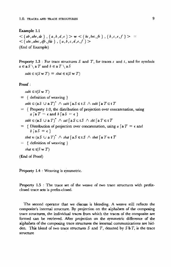
Example 1.1

< { ab , abc , de } , { a , b , d, c } > w < { bc , bcc ,ft } , { b , c , c ,J } > < { abc, abec, dfc ,jde } , { a , b , c, d, e ,J } > (End of Example)

9

Property 1.3 : For trace structures S and T, for traces s and t, and for symbols a E aS \ a T and b E a T \ aS

sabt E t(S w T) = sbat E t(S w T)

Proof :

sabt E t(S w T)

= { definition of weaving }

sabte(aS U aT)• 1\sabtfaSetS 1\ sabtfaTetT

= { Property 1.0, the distribution of projection over concatenation, using a fa T = t: and b fa S = t: }

sabte(aS U aT)• 1\satfaSetS 1\ sbtfaTetT

= { Distribution of projection over concatenation, using a fa T = t: and b f aS = t:}

sbate(aS U aT)• 1\sbatfaSetS 1\ sbatfaTetT

= { definition of weaving }

sbat e t(S w T)

(End of Proof)

Property 1.4 : Weaving is symmetrie.

Property 1.5 : The trace set of the weave of two trace structures with prefix­closed tracesets is prefix-dosed.

The second operator that we discuss is blending. A weave still refiects the composite's internal structure. By projection on the alphabets of the composing trace structures, the individual traces from which the traces of the composite are formed can be retrieved. After projection on the symmetrie difference of the alphabets of the composing trace structures the internal communications are hid­den. This blend of two trace structures S and T, denoted by S b T, is the trace structure

10 TRACE THEORY

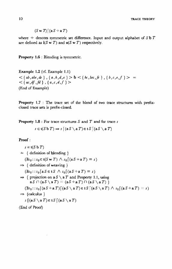
(Sw7)f(aS+aT)

where ...;- denotes symmetrie set difference. Input and output alphabet of S b T are defined as i(S w T) and o(S w T) respectively.

Property 1.6 : Blending is symmetrie.

Example 1.2 ( cf. Example 1.1)

< { ab , abe , de } , { a , b , d, e } > b < { bc , bec ,je } , { b , c, e ,j } > < { ac, 4f ,jd } , { a , c, d ,j } > (End of Exarnple)

Property 1.7 : The trace set of the blend of two trace structures with prefix­closed trace sets is prefix-closed.

Property 1.8 : Fortrace structures S and T and fortraces

s E t(S b T) ~ s f (aS \ a T) E t S f (aS \ a T)

Proof:

sE t(SbT)

= { definition of blending }

(3s o : : s o E t( S w T) 1\ s o f (aS ...;-a T) = s )

~ { definition of weaving }

(3s o : : s o fa S E t S 1\ s o f (aS ...;-a T) = s )

~ { projection on aS \a T and Property 1.1, using aS n (aS \ a T) = (aS ...;-a T) n (aS \ a T) }

(3s0 ::s0 f(aS+aT)f(aS\aT)EtSf(aS\aT) 1\ s0 f(aS+aT) = s)

~ {calculus }

s f(aS \a T)E tS f(aS \aT)

(End of Proot)

1.1. A PROGRAM NOTATION 11

l.l. A program notation

In this section we discuss a way to represent trace structures. Since trace sets are often infinite, a representation by enumeration of its elements becomes rather cumbersome. We use so-called commands with which we associate trace struc­tures. With command S trace structure TRS is associated in the following way.

-A symbol is a command. For symbol a TRa = < {a} , {a}>.

- If S and T are commands then ( S I T) is a command. TR(S I T) = < t(TRS) U t(TR T), a(TRS) U a(TR T) >.

- If S and T are commands then (S ; T) is a command. TR(S ; T) = < {x ,y : x E t (TR S) Á y E t (TR T) : -91 } , a (TR S) U a (TR T) >.

- If S and T are commands then (S, T) is a command. TR(S,T) = (TRS)w(TRT).

- If s is a command then s· is a command. TR(S•) = < (t(TRS))• , a(TRS) >

Furthermore, there are a few priority rules. The star has the highest priority, fol­Iowed by the comma, the semicolon, and the bar. The trace sets thus obtained are not prefix-closed. Since we are interested in prefix-closed trace sets only, as will turn out in the next chapter, we associate with a command S the trace structure < pref(t (TR S)) , a (TR S) >, when the command is used for the specification of a mechanism.

Example 1.3

The specification of a Wire, as exemplified in Example 1.0 would be input alphabet {a } , output alphabet { b } , and command (a ; b) •.

(End of Example)

Example 1.4

A Muiler-G element, or Gelement for short [6], is an element with two inputs and one output. lt is supposed to synchronize the inputs, i.e. after having received an input change on both input wires, it produces a change on the out­put wire. lts specification is a trace structure with input alphabet {a, b }, output alphabet { c }, and command (a, b ; c) •.

(End of Example)

2 Classification of delay-insensitive trace

structures

With the trace theory as introduced in the preceding chapter we are now able to define delay-insensitive trace structures formally. We reserve the term com­ponent for a mechanism that is an abstraction of an dectrical circuit. A trace structure is the specification of the communications between a component and its environment. Inputs of the trace structure are inputs with respect to the com­ponent and outputs with respect to the environment. Outputs of the trace struc­ture are outputs with respect to the component and inputs with respect to the environment.

The key to the definition of delay-insensitive trace structures is the component and its environment being insensitive to the speeds with which they operate and to propagation delays in connecting wires. This is informally captured by view­ing a component as being wrapped in some kind of foam box representing a flexible and possibly time-varying boundary. The communication actions between component and environment are specified at this boundary. The flexi­bility of this boundary imposes certain restrictions that the specification of a delay-insensitive circuit has to satisfy. As will turn out in the sequel, these requirements basically amount to the absence of ordering between certain sym­bols : the presence of certain traces in a trace structure's trace set implies the presence of other traces in that trace set. It is not a priori obvious that the requirements deduced in this chapter on account of this foam rubber wrapper principle are sufficient to guarantee proper communications. This will only turn

out in Chapter 4. The first restrietion to be imposed upon a trace structure is that its alphabet

be partitioned into an input and an output alphabet. We do not, at this level of abstraction at least, consider a communication means other than input or out­put, nor do we çonsider ports that are input at one time and output at another

12

13

time. This means that we have for trace structure T the rule

R 0) i T U o T = a T

Notice that i T n o T = 0 according to the definition of a trace structure. Second, we impose the restrietion that a trace set he prefix-closed and non­

empty. This rule is dictated by the fact that a system that can produce trace ta is assumed to do so by first producing t and then a . The symbols in a trace structure's alphabet are viewed as atomie actions. Moreover, a system must he able to produce € initially. This gives for trace structure T the rule

R 1) t T is prefix-closed and non-empty

The basic idea of this monograph is that we do not make any assumptions on absolute or relative wire delays. As we pointed out in the introduction, this leads to the assumption of a transition being monotonic in order to enable a com­ponent to recognize the signal that this transition represents. This means that we have to guarantee transitions against interference and, therefore, have to limit the number of transitions on a wire to at most one. In terms of trace structures, where signals via the same wire are represented by the same symbol, this arnounts to the restrietion that adjacent symbols he different. This gives for trace structure T the following necessary condition.

R 2) for trace s and symbol a E a T saa fl t T

Signals are sent in either of two directions, viz. from a component to its environment or the other way round. Due to unknown wire delays, two signals being sent the one after the other in the same direction via different wires need not he received in the order in which they are sent. In other words, we cannot assume our communications to he order preserving. Consequently, a specification of a delay-insensitive component does not depend on the order in which this kind of concurrent signals is sent or received. Therefore, a trace structure con­taining a trace with two adjacent symbols of the same type (input or output) also contains the trace with these two symbols swapped. In fact, we conceive adjacent symbols of the same type as not being ordered at all. (Their occurrence as adjacent symbols in a trace is just a shortcorning of our writing in a linear way.) Fortrace structure T, this is expressed by the following restrietion

R 3) for traces s and t, and for symbols a E a T and b E aT of the same type saht E t T = sbat E t T

Due to the foarn rubber wrapper principle, signals in opposite directions are subject to restrictions as well. As opposed to signals of the same type, they may

14 CLASSIFICATION OF DELAY INSENSITIVE TRACE STRUCTURES

have a causa! relationship and, hence, have an order. If, however, insome phase of the computation they are not ordered, meaning that for some trace s and symbols a and b both sa E t T and sb E t T, then the traces that sab and sba can be extended with, according to the camponent's trace set, should not differ tob much. Obviously, we do justice to the faam rubber wrapper principle if the order of this kind of concurrent symbols is of no importance at all. This results for trace structure T in the rule

R 4') fortraces s and t, and for symbols a E aT and bEaT of different types sa E t T 1\ sbat E tT ~ sabt E t T

Finally, we have to take into account that a signa!, once sent, cannot be can­celled. However long it takes, eventually it wil! reach its destination. Conse­quently, a component ready to receive a certain signa! from its environment, which means that the trace thus far generated extended with that symbol belongs to the trace set, must not change its readiness when sending a signa! to its environment. In other words, in the absence of an oracle infonning either side on signals that, though possible, will not be sent, we cannot allow in a specificatien that a symbol elisables a symbol of another type. Symbol a elisables symbol b in trace structure T if there is a trace s with

sa E t T 1\ sb E t T 1\ sab f/: t T

There is nothing wrong, however, with symbols that elisabie symbols of the same type. If these symbols are input symbols then the environment has to make a decision which output symbol(s) to send. If, on the contrary, the symbols are output symbols then the component has to make that decision. Since a correct use of arbitration devices is one of the important incentives to the study of delay-insensitive circuits, the various types of decisions are a key to the classification. Three classes, each of them described by one of the following non­elisabling rules, can be distinguished now. For trace structure T we have

R 5') for trace s and distinct symbols a E a T and b E a T sa E t T 1\ sb E t T ~ sab E t T

R 5") fortraces and distinct symbols a E aT and bEaT, notbath input sym­bols, sa E t T 1\ sb E t T ~ sab E t T

R 5"') for trace s and symbols a E a T and b E a T of different types sa E t T 1\ sb E t T ~ sab E t T

All delay-insensitive trace structures satisfy R 0 through R 3. The class satisfy­ing R 4' and R 5' as well is called the synchronization class. lt is also denoted by C 1• A specificatien in this class allows for synchronization only. Due to the

15

absence of decisions, no data transmiSSIOn is possible. The class allowing for input symbols to be disabled, satisf)'ing therefore R 4' and R 5", is called the data communication class. It is also denoted by C 2• Here the data is encoded by means of the possible decisions. Finally, we have C 3, or the arbitration class, which allows a component to choose between output symbols. Specifications in this class satisfY, in addition to R 0 through R 3, R/ and R 5"'. Obviously, c,cc 2 cC3.

We could have distinguished the class in which decisions are made in the component and not in the environment, which is C 2 with in its R 5" the restrie­tion 'not both inputs' replaced by 'not both outputs'. We havenotclone so, how­ever, since none of the classes thus obtained turns out to be closed under the composition operator proposed in the next chapter, a circurnstance rnaicing none of these classes very interesting. C 3 has, arbitrarily, been chosen to demonstrate this phenomenon.

The reason that C 3 is not closed under composition is that R/ is too restric­tive in the presence of decisions in the component, as is shown in Chapter 5. We concluded the analysis for R/ by observing that the foam rubber wrapper prin­ciple would certainly be clone justice if the order of concurrent symbols of different types was of no importance. This situation, however, needs a more care­ful analysis.

The specification of a component must not depend on the place of the boun­dary of the foam rubber wrapper. Consider two wrappers, the one contained in the other one. lf, at the outside boundary the order between two concurrent input and output signals is input-before-'output, then nothing can be said about their order at the inside boundary. If, on the other hand, the order between such signals is output-before-input at the outside boundary, then the same order between these symbols is implied at the inside boundary.

The first situation, i.e. input-before-output at the outside boundary, gives rise to a restrietion to be imposed upon a camponent's trace set. Assume that we have traces s and t, input s}rmbol a , output symbol b , and traces sabt and sbat in the camponent's trace set. Trace sabt is the trace associated with the outside boundary and trace sbat is the one that is associated with the inside boundary. Now if sabt can be extended -according to the camponent's trace set- with an input symbol c, which means a signa! from the outside boundary towards the inside boundary, then a necessary condition for absence of computation interfer­ence at the inside boundary is the presence of trace sbatc in the camponent's trace set.

A similar observation applies to an output-before-input order of concurrent symbols at the inside boundary and an input-before-output order at the outside boundary. In this case an output signa! possible at the inside boundary should be possible at the outside boundary as wel!. This results for trace structure T in the following rule, which is less restrictive than R/.

16 CLASSIFICATION OF DELAY INSENSITIVE TRACE STRUCTURES

R 4") for traces s and t, and for symbols a E aT, bEaT, and c E aT with b of another type than a and c sabtc E t T 1\ sbat E t T ~ sbatc E t T

R 0 through R 3 together with R 4" and any of the three R 5's constitute a class of delay-insensitive trace structures. We give a name to the largest class only, which is the one with R 4" and R 5"'. We call it the class of delay-insensitive trace structures and denote it by C 4. Obviously, C 3 c C 4• We do not attach narnes to the other classes, since these classes neither provide more insight nor have surprising properties.

Before exploring R 4", we illustrate this classification by a nwnber of exam­ples. In these examples we sometimes represent a trace structure by a state graph instead of by a command. A state graph is a directed graph with one spe­cial node, the start node, and arcs labelled with symbols of the trace structure's alphabet. Each path from the start node corresponds to a trace, viz. the one that is brought a bout by the labels of the consecutive arcs in that path. A state graph is said to represent a trace structure if it has the same trace set as that trace structure. Rules R 3, R 4', and R 5 are usually more easily checked in a state graph than in a command. Rule R 4" is hard to check in either representation. In the figures the start nocles are drawn fat . Choosing another node as start node means another initialization of the component. Components that only differ from one another by different start nocles are given the same name. For clear­ness' sake we attach a question mark to arcs labelled with an input symbol and an exclamation mark to arcs labelled with an output symbol.

Example 2.0

The Wire and the C-element of Examples 1.3 and 1.4 are C 1 's. Interchanging the roles of the input and the output alphabet yields C 1's again. The wire remains a wire, now starting with an output however. The C-element becomes a Fork, viz. a trace structure with input alp ha bet { c } , output alphabet {a, b } , and command (a , b ; c) • . By another initialization we also have the command (c ;a , b)" fora Fork.

(End of Example)

Example 2.1

Another very common element is the so-called Merge. I t is an element with input alphabet {a,b}, output alphabet {c }, and command ((a I b);c)·. This component is a C 2, since inputs a and b disable one another. Interchanging the roles of input and output alphabet yields a C 3. This is the simplest form of an arbiter.

(End of Example)

17

Example 2.2

A C-element with two outputs instead of one is another example of a C 1• lt has input alphabet {a, h } and output alphabet { c, d } . There are two essentially different trace structures that synchronize the input signals. The first one is the C-element with its output symbol replaced by two output symbols in any order. This yields command (a , h ; c , d) • . In this trace structure we can distinguish an input and an output phase. Another command allows the two phases to overlap a little bit, but still synchronizes the inputs. This is expressed in the command a,h; ((c ;a),(d; h))".

(End of Example)

Example 2.3

Consider a C-element with input alphabet {a, r } , output alphabet { p } , and command (a ,r ;p )" and consider a Wire with input alphabet { q }, output alphabet { h }, and command (q; b)". The Wire can be used to acknowledge the reception of symbol p by the environment before a next input a is allowed to occur. The resulting component has input alphabet {a, q, r } , output alphabet { h ,p }, and command a ; (p ; (q ; h ; a), r )". We have chosen this initiali.zation, since the component will be used in this form in Chapter 5. It is a C 1•

(End of Example)

Example 2.4

Another component that will be used in Chapter 5 is a component that can be thought of as consisting of three wires : two wires to convey a bit of information and one wire for the acknowledgement of its arrival. A bit is encoded as sending a signa! on one of the two wires that are used for the data transmission. lts input alphabet is {x 0 , x 1 , h } , its output alphabet is {Jo ,J 1 , a } , and its command is (x 0 ;Jo ; h; a I x 1 ;J 1 ; h; a)". Because of the choice to be made between the inputs Xo and X1 this COmponent is a C2.

(End of Example)

Example 2.5

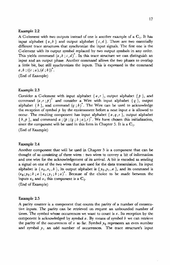
A parity counter is a component that counts the parity of a number of consecu­tive inputs. The parity can be retrieved on request an unbounded number of times. The symbol whose occurrences we want to count is x. lts reception by the component is acknowledged by symbol a . By means of symbol h we can retrieve the parity of the occurrences of x so far. Symbol Jo represents an even number and symbol J 1 an odd number of occurrences. The trace structure's input

18 CLASSIFICATION OF DELAY INSENSITIVE TRACE STRUCTURES

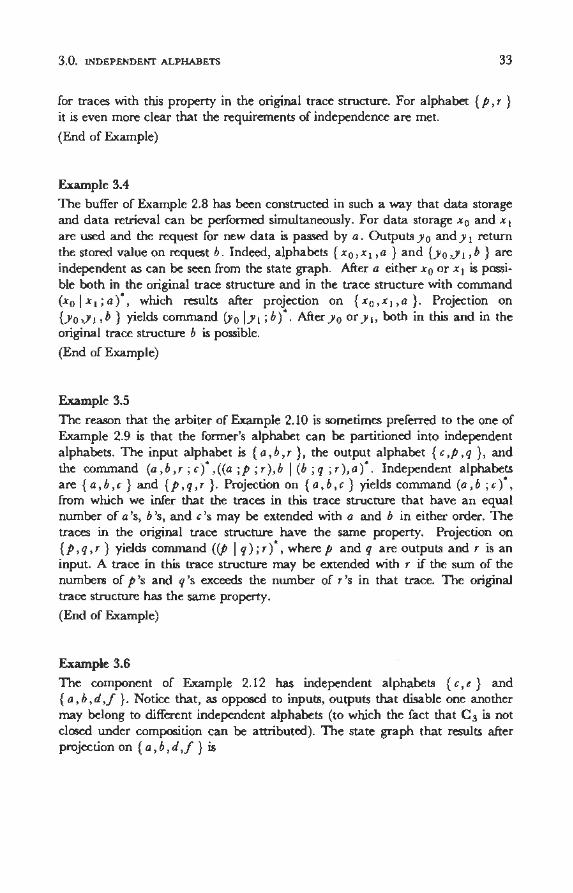
alphabet is {x, b }, its output alphabet is {a ,y0 ,y1 }, and its conunand is ((b ;yo)· ;x ;a; (b ;y.)· ;x ;a)·. This component is a c2. There is a choice to be made between inputs x and b. To show that more clearly we draw a state graph of this component.

n;:--·--z.n • • • • •

b? a! x? b?

Any two arcs from the same node have labels of the same type, which implies that R 4' is trivially satisfied. There are no two consecutive arcs with labels of the same type, which implies that R 3 is satisfied. Any two arcs from the samenode have labels of type input that do disable one another. This does not meet requirement R 5', but this is allowed according to R 5". Consequently, this is a C2.

(End of Example)

Example 2.6

An And-element with input alphabet {a, r } and output alphabet { c } is quite often used in the following way. Both inputs go high in some order whereafter the output follows the inputs. Next, both inputs go low again and the output fol­lows the first low-going input transition. This is expressed by the command (a, r ; c ; (a ; (c ,r) I r ; (a, c )) •. This trace structure is not delay-insensitive, how­ever. It contains, for instance, the trace arcrcaa, which violates R 2. lt can be made delay-insensitive by replicating both inputs. Then its input alphabet is { a, r } , its output alphabet { b, c ,p } and a possible command (a ; p ; r ; b ,c; a; c ,(p; r; b ))•. Input a is now acknowledged by p and r by b. It is not the most general conunand for a delay-insensitive And-element but one that suffices for the sequel. The corresponding trace structure is a C 1•

(End of Example)

Example 2.7

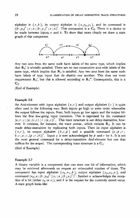
A binary variabie is a component that can store one bit of information, which may be retrieved afterwards on request an unbounded number of times. The component has input alphabet {x0 ,x1 ,b }, output alphabet {y 0 ,y1 ,a }, and conunand (x0 ; a; (b ;y0)• I x 1 ; a ; (b ;y 1)" )•. Symbol a acknowledges the recep­tion of a bit (either x 0 or x 1), and b is the request for the currently stored value. A state graph looks like

19

b? a!

·"--J·~· Yo! xo?

Inthestart node a choice has to he made between x0 and x 1 (it has no currently stored value). Moreover, there are two nodes where a choice has to he made between inputs b, Xo, and X1. This makes it a C2.

(End of Example)

Example 2.8

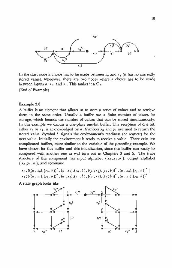
A buffer is an element that allows us to store a series of values and to retrieve them in the same order. Usually a buffer has a finite number of places for storage, which bounds the number of values that can he stored simultaneously. In this example we ruscuss a one-place one-bit buffer. The reception of one bit, either x 0 or xh is acknowledged by a. Symbolsy0 andy 1 are used to return the stored value. Symbol b signals the environment's rearuness (or request) for the next value. Initially the environment is ready to receive a value. There exist less complicated buffers, more similar to the variabie of the preceding example. We have chosen for this buffer and this initialization, since this buffer can easily he composed with another one as will turn out in Chapters 3 and 5. The trace structure of this component has input alphabet { x0 , x 1 , b } , output alphabet {yo,Yt ,a}, and command

x o ; ( ( (a ; x o), (y o ; b)) • ; (a ; x 1), (y 0 ; b) ; ( (a ; x 1) , (y 1 ; b ) )" ; (a ; x o), (y 1 ; b) )" I x 1 ; (((a ; x 1), (y 1 ; b ))" ; (a ; xo), (y 1 ; b); ((a ; xo), CYo; b )) • ; (a ; x 1), CYo; b ))"

A state graph looks like

2~::::J ! xo? • x1? 2i~ • • . l . j 1/1 1''' I '·'I i'J •

JJ}' "l~l •

j j ./. • • • • 1 xo? a! a! x1? 2

20 CLASSIFICATION OF DELAY INSENSITIVE TRACE STRUCTURES

We have not labelled all arcs. Opposite sides of the parallelograms have equal labels. Nodes that have been attached the same number are identical. Here we see the existence of a node with outgoing arcs with labels of different types. It is easy to see that R 4' is still satisfied, since arcs with such labels make up a paral­lelogram, which means that their order is of no importance. This component is a C2, the only decision tO he made being the One between inputs Xo and X1.

(End of Example)

Exarnple 2.9

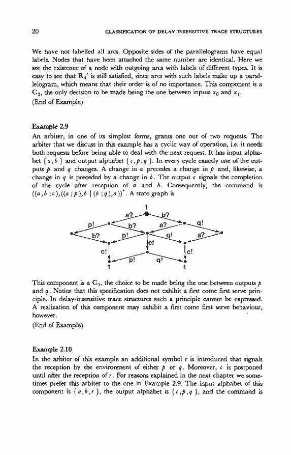
An arbiter, in one of its simplest forms, grants one out of two requests. The arbiter that we discuss in this example has a cyclic way of operation, i.e. it needs both requests before being able to deal with the next request. It has input alpha­bet {a, b } and output alphabet { c ,p, q } . In every cycle exactly one of the out­puts p and q changes. A change in a preeerles a change in p and, likewise, a change in q is preeerled by a change in b. The output c signals the completion of the cycle after reception of a and b. Consequently, the command is ((a ,b j c ),((a ;p ),b I (b j q ),a n· 0 A state graph is

1

___51----·~ ~-~Y--·~

·----- b? p!---i~ __51---. ~ • ......-:- ~c! •

c!! __..--•--. te! • .------p! q! ~. 1 1

This component is a C 3, the choice to he made being the one between outputs p and q . Notice that this specification does not exhibit a first come first serve prin­ciple. In delay-insensitive trace structures such a principle cannot he expressed. A realization of this component may exhibit a first come first serve behaviour, however.

(End of Example)

Example 2.10

In the arbiter of this · example an additional symbol r is introduced that signals the reception by the environment of either p or q. Moreover, c is postponed until after the reception of r. For reasons explained in the next chapter we some­times prefer this arbiter to the one in Example 2.9. The input alphabet of this component is {a, b, r }, the output alphabet is { c ,p, q }, and the command is

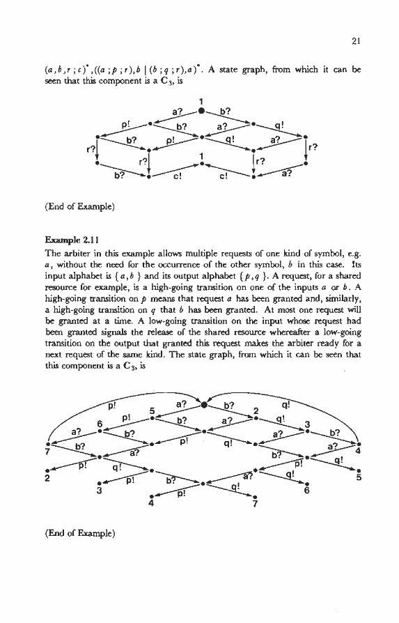
21

(a,b,r;c)",((a;p;r),b l(b;q;r),a)" . A state graph, from which it can be seen that this component is a c3, is

(End of Example)

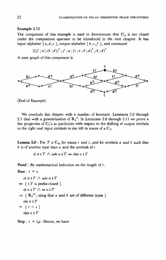
Example 2.11

The arbiter in this example allows multiple requests of one kind of symbol, e.g. a, without the need for the occurrence of the other symbol, b in this case. lts input alphabet is {a, b } and its output alphabet { p, q } . A request, for a shared resource for example, is a high-going transition on one of the inputs a or b . A high-going transition on p means that request a has been granted and, similarly, a high-going transition on q that b has been granted. At most one request will be granted at a time. A low-going transition on the input whose request had been granted signals the release of the shared resource whereafter a low-going transition on the output that granted this request makes the arbiter ready for a next request of the same kind. The state graph, from which it can be seen that this component is a C 3, is

p! 5~·~2 q!

6~·~ __51---·~3 ~·~ ..---or-·~ __51---·~

• ----b? ---.:::--• p. q · ·----- a1---• 7 ---.... __.-a? b??---.... .---- . 4 ----r--•--.,__ . • Cl I .---- p! q! ---..... ._:----r ~. 2 ~~~~ 5 . ----·----g! .

3 • .......---p! --.......__. 6 4 7

(End of Example)

22 CLASSIFICATION OF DELAY INSENSITIVE TRACE STRUCTURES

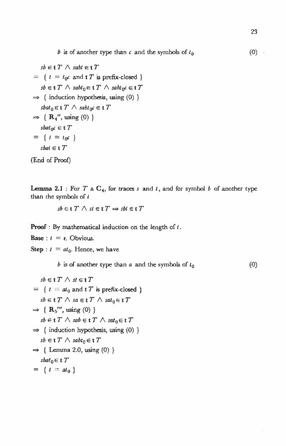
Example 2.12

The component of this example is used to demonstra te that C 3 is not closed under the composition operator to he introduced in the next chapter. It has input alphabet { a, d, e } , output alphabet { b, c J } , and conunand

(((j ; a), (b ; d)) • ;J ; a ; (c ; e ; b ; d)" ; b ; d)"

A state graph of dus component is

(End of Example)

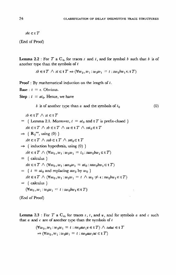
We conclude this chapter with a number of lemmata. Lenunata 2.0 through 2. 7 -deal with a generalization of R 4". In Lenunata 2.8 through 2.11 we prove a few properties of C 2 's in particular with respect to the shifting of output symbols to the right and input symbols to the left in traces of a C 2•

Lemma 2.0 : For T a C 4, fortraces s and t, and for symbols a and b such that b is of another type than a and the symbols of t

sb E t T 1\ sabt E t T ~ sbat E t T

Proof : By mathematica! induction on the length of t.

Base: t = f.

sb E t T 1\ sabt E t T

~ { t T is prefix-closed }

sb E t T 1\ sa E t T

~ { R 5"', using that a and b are of different types }

sba Et T

= { t = (} sbat Et T

Step : t = t0c. Hence, we have

b is of another type than c and the syrnbols of t0

sb E t T 1\ sabt E t T

= { t = t 0c and t T is prefix-closed }

sb E t T 1\ sabt0 E t T 1\ sabt0c E t T

=> { induction hypothesis, using (0) }

sbat0 Et T 1\ sabt0c Et T

=> { R 4", using (0) }

sbatoe Et T

= { t = toe }

sbat Et T

(End of Proof)

23

(0)

Lemma 2.1 : For T a C 4 , for traces s and t, and for syrnbol b of another type than the syrnbols of t

sb E t T 1\ st E t T => sbt E t T

Proof : By mathematical induction on the length of t .

Base : t = t:. Obvious.

Step : t = at0• Hence, we have

b is of another type than a and the syrnbols of t0

sb E t T 1\ st E t T

= { t = at0 and t T is prefix-closed }

sb Et T 1\ sa Et T 1\ sat0 Et T

=> { R 5"', using (0) }

sb E t T 1\ sab E t T 1\ sat0 E t T

=> { induction hypothesis, using (0) }

sb E t T 1\ sabt0 E t T

=> { Lemma 2.0, using (0) }

sbat0 E t T

= { t = at0 }

(0)

24 CLASSIFICATION OF DELAY INSENSITIVE TRACE STRUCTURES

sbt Et T

(End of Proof)

Lemma 2.2 : For T a C 4, fortraces s and t, and for symbol b such that b is of another type than the symbols of t

sb Et T 1\ st Et T ~ ('iw0 ,w1 : WoW I = t :sw0bw 1 Et T)

Proof : By mathematica! induction on the length of t.

Base : t = L Obvious.

Step : t = at0. Hence, we have

b is of another type than a and the symbols of t 0

sb E t T 1\ st E t T

= { Lemma 2.1. Moreover, t = at0 and t T is prefix-closed }

sbt Et T 1\ sb Et T 1\ sa Et T 1\ sat 0 Et T

~ { R 5"', using (0) }

sbt E t T 1\ sab E t T 1\ sat0 E t T

~ { induction hypothesis, using (0) }

sbt Et T 1\ ('iw0 ,w1 : w 0w 1 = t 0 : saw0bw1 Et T)

= { calculus }

sbt Et T 1\ ('iw0 , w 1 : aw0w 1 == at0 : saw0bw 1 Et T)

= { t = at0 and replacing aw0 by w 0 }

sbt E t T 1\ ('iw0 ,w1 : w 0w 1 = t 1\ w 0 =Ft:: sw0bw 1 Et T)

= { calculus }

('iw0 ,w 1 : w 0w 1 = t: sw0bw 1 Et T)

(End of Proof)

(0)

Lemma 2.3 : For T a C 4, for traces s, t, and u, and for symbols a and c such that a and c are of another type than the symbols of t

('iw0 ,w1 : w 0w 1 = t : swoaw 1u Et T) 1\ satuc Et T

~ ('iw 0 ,w1 :w0w 1 = t :swoaw1uc EtT)

Proof : By mathematica! induction on the length of t.

Base : t = t:. Obvious.

Step : t = bt0• Hence, we have

a and c are of another type than b and the symbols of t0

('Vwo ,wi: WoW! = t: swoaw,u Et T) 1\ satuc Et T

= { t = bt0 }

('Vw 0 ,w1 : w0w 1 = bt0 : swoaw 1u Et T) 1\ sabtoue Et T

==> { calculus }

('Vw0 ,w 1 : w 0w 1 = t 0 : sbwoaw 1u Et T) 1\ sbat0u Et T 1\ sabt0uc Et T

==> { R,.'', using (0) }

('Vw0 ,w1 : WQW 1 = t0 : shwoaw 1u Et T) 1\ sbat0uc Et T 1\ sabt0uc Et T

==> { induction hypothesis, using (0) }

('Vw 0 , w 1 : w 0w 1 = t 0 : sbwoaw 1uc Et T) 1\ sabtoue Et T

= { calculus }

('Vwo ,w, :WoW I = hto 1\ Wo =I= (: swoaw,uc Et T) 1\ sahtouc Et T

= { calculus and t = bt0 }

('Vw 0 ,w1 : w0w 1 = t : sw0aw 1uc Et T)

(End of Proof)

In exactly the same way we derive

25

(0)

Lemma 2.4 : For T a C 4, fortraces s, t, and u, and for symbols b and c such that b is of another type than c and the symbols of t

('Vwo, w 1 : w0w 1 = t : sw0bw 1u Et T) 1\ stbuc Et T

==> ('Vw0 ,w 1 : w0w 1 = t : sw0bw 1uc Et T)

Lemma 2.5 : For T a C 4, fortraces s, t, and u, and for symbol a such that a is of another type than the symbols of t

satu Et T 1\ stau Et T ==> ('Vw0 ,w1 : WQW 1 = t :swoaw 1u Et T)

Proof : By mathematical induction on the length of u.

26 CLASSIFICATION OF DELAY INSENSITIVE TRACE STRUCTURES

Base: u = t:. satu E t T 1\ sûzu E t T

~ { t T is prefix-closed }

saEtT 1\stEtT

~ { Lemma 2.2, since a is of another type than the symbols of t

('v'w0 ,w1 :w0w 1 = t :sw0aw 1 EtT)

~ {u = t:}

('v'wo ,wl : WoW! = t: swoawlu Et T)

Step: u = u0b.

satu E t T 1\ sûzu E t T

= { u = u0b and t T is prefix-closed }

satu0 Et T 1\ sûzu0 Et T 1\ satu0b Et T 1\ sûzu0b Et T

~ { induction hypothesis }

('v'wo, w I :WoW I = t : swoaw luo Et T) 1\ satuob Et T 1\ sûzuob Et T

~ { Lemma 2.3 if the types of a and b are equal, Lemma 2.4 if they are not }

('v'wo, wl :WoW! = t : swoawluob Et T)

= {u = u0b }

('v'w 0 ,w1 :woW 1 = t :sw0aw 1u EtT)

(End of Proof)

Lemma 2.6 : For T a C 4, for traces s, t, and u, and for symbols a and c such that the symbols of t are of another type than a and c

satuc E t T 1\ sûzu E t T ~ stauc E t T

Proof:

satuc E t T 1\ stau E t T

= { t T is prefix-closed }

satu E t T 1\ sûzu E t T 1\ satuc E t T ~ { Lemma 2.5 }

('v'wo ,wl: WoW! = t : swoawlu Et T) 1\ satuc Et T

~ { Lemma 2.3 }

('v'w 0 ,w1 :woW 1 = t:swoaw 1ucEtT)

~ { instantiation }

stauc Et T

(End of Proof)

In a sirnilar way, applying Lemma 2.4 instead of 203, we derive

27

Lemma 2. 7 : For T a C 4, for traces s, t , and u, and for symbols b and c such that b is of another type than c and the syrnbols of t

stbuc E t T Á sbtu E t T ~ sbtuc E t T

Finally we prove a few lemmata on the shifting of syrnbols in C 2'so

Lemma 2.8 : For T a c2, for traces s and t' and for syrnbol a E 0 T such that tr{a}=t:

sa E t T Á st E t T ~ sta E t T

Proof : By mathematica! induction on the length of t 0

Base : t = t:. Obviouso

Step : t = t 0b 0 Hence, we have

tor {a } = t: and a =F b

sa E t T Á st E t T

= { t = t0b and t T is prefix-closed }

sa E t T Á st0 E t T Á st0b E t T

~ { induction hypothesis, using (0) }

stoa E t T A st0b E t T

~ { R 5", using a E o T and a =F b according to (0) }

st0ba Et T

= { t = t 0b }

sta Et T

(End of PrOQf)

(0)

28 CLASSIFICATION OF DELAY INSENSITIVE TRACE STRUCTURES

Lemma 2.9 : For T a C 2, for traces s, t, and u, and for symbol a E o T such that t r { a } = f

sa E t T 1\ stau E t T => satu E t T

Proof : By mathematica! induction on the length of t.

Base : t = f. Obvious.

Step : t = t0b. Hence, we have

tor { a } = f and a =I= b

sa E t T 1\ stau E t T

= { t = t0b and t T is prefix-dosed }

sa E t T 1\ st0 E t T 1\ st0bau E t T

=> { Lenuna 2.8, using (0) and a E o T }

sa E t T 1\ stoa E t T 1\ st0bau E t T

=> { R 4' if a and b are of different types, R 3 if they are of the same type }

sa Et T 1\ stoabu Et T

=> { induction hypothesis, using (0) }

sat0bu Et T

= { t = t 0b }

satu Et T

(End of Proof)

(0)

Lemma 2.10 : For T a C 2, fortraces s, t, and u, and for symbol a E o T such that t r { a } = f

sa Et T 1\ stau Et T =>('Vwo ,w,: WoW! = t : swoaw,u Et T)

Proof:

sa E t T 1\ stau E t T = { t T is prefix-closed and calculus }

(\fw0 ,w1: w0w 1 = t :sa E t T 1\ sw0 E t T 1\ sw0w 1au Et T)

=> { since t r {a } = f, we have, if WoW! = t' Wo r {a } = f. Hence, we may apply Lenuna 2.8 }

(\fwo,w 1: WoW! = t :swoa Et T 1\ sw0w 1au Et T)

~ { Lemma 2.9 }

('v'w 0,w1 :w0w 1 = t :sw0aw 1u EtT)

(End of Proof)

Lemma 2.11 : ForT a c2, fortraces s' t' and u' and for symbol a Ei T

('v'wo ,WJ : WoW I = t : swoa Et T) A stau Et T

~ ('v'w 0,w 1 :w0w 1 = t :swoaw 1u EtT)

Proof : By mathematical induction on the length of t .

Base : t = t. Straightforward.

Step : t = t 0b . Then we derive

('v'w0,w1: w0w 1 = t :swoa Et T) A stau Et T

= { t = t0b }

('v'wo , wl : WoW! = tob : swoa Et T) A stobau Et T

~ { calculus }

(V' wo' w I : WoW I = to : swoa E t T) A stoa E t T A stobau E t T

~ { R 3 if a and b are of the same type. R 4' if they are of different types }

('v'wo ,wl: WoW I = to : swoa Et T) A stoabu Et T A stobau Et T

~ { induction hypothesis }

('v'wo,WI: WoW I = to : swoawlbu Et T) A stobau Et T

= { calculus }

('v'w 0 ,w 1 : w0w 1 = t0b A w 1 =I= t: swoaw 1u Et T) A st0bau Et T

= { calculus and t = t 0b }

('v'w0, w 1 :w0w 1 = t :swoaw1u EtT)

(End of Proof)

29

3 Independent alphabets and composition

In dus chapter we introduce so-called independent alphabets. Infonnally speak­ing, we particion the environment of a component in such a way that the suben­vironments are mutually independent with respect to their communications with that component. Such a partitioning is, for example, a justification for sometimes conceiving the environment as being divided into a left and a right environment. In the last section a compositi<?n operator is defined using independent alpha­bets.

3.0. Independent alpbahets

Outputs of the component are under control of the component and inputs of the component are under control of the environment. The component will operate according to its specification by sending outputs as long as the environment sends outputs that the component is able to receive according to that specification, in other words as long as there is absence of computation interfer­ence.

Composition of two dectrical circuits usually involves the interconnection of just a subset of wires of the circuits to be composed. Communications via these wires are the composite's intemal communications. The remaining wires are used for the external communications, i.e. the communications of the composite with its environment. Therefore, the environment of each component is partitioned, upon composition, into an environment for the internal and an environment for the extemal communications. This implies two so-called local specifications, viz. the one obtained by projecting the original specification onto the symbols used for the internal communications and the one obtained by projecting onto the symbols used for the extemal communications. A nice property of dUs partition­ing would be that the intemal and extemal communications could be carried

30

3.0. INDEPENDENT ALPHABETS 31

out according to the rules of the preceding paragraph just with respect to their local specifications, i.e. by locally guaranteeing absence of computation interfer­ence guaranteeing absence of computation interference for the whole. This is captured. in the requirement that if an input symbol is allowed to occur accord­ing to a local specification then it is also allowed to occur according to the glo­bal one. Formally this is defined as follows.

Definition 3.0 : For T a C 4, alphabet C, C ç aT, is independent with respect toT if

(V s, a : s E t T (\ a E C n i T : sa f C E t T f C = sa E t T) (\

(V s, a : s E t T (\ a E C n i T : sa f C E t T f C = sa E t T)

where the complement of C with respect to a T is denoted by C.

(End of Definition)

Notice that aT itself is independent with respect to trace structure T. The equality could be replaced by an implication since sa E t T => sa r c E t T r c by definition. Moreo~er, it can be seen that independenee of C is the same as independenee of C.

One of the requirements for composition of two components will be that their set of common symbols be independent with respect to bath components. This is sufficient to guarantee absence of computation interference as far as external input symbols are concerned, as will be proved in Lemma 3.5. Additional requirements are needed to guarantee absence of computation interference for the internal inputs. First, however, we illustrate the definition of the notion of independent alphabet using some examples of the preceding chapter.

Example 3.0

Consider a C-element with two output wires as in Example 2.2. The input alphabet is {a, b }, the output alphabet is { c, d }. The cómponent with cam­mand a ,b ; ((c ; a), (d; b ))• has independent alphabets {a, c } and { b ,d }. Pro­jection on { a , c } yields a trace structure with cammand (a ; c ) • . The traces in this trace structure that contain an equal number of a 's and c's may be extended with a. Traces of the original trace structure with an equal number of a's and c's may be extended with a as well, as can easily be seen from the cam­mand. For reasans ofsymmetry, sarnething similar holds for alphabet { b,d }. Taking the component with cammand (a ,b; c ,d)•, however, one cannot find independent alphabets other than the trivial ones. Trace abc in this trace struc­ture, for instance, cannot be extended with a , although its projection on { a , c } ,

32 INDEPENDENT ALPHABETS AND COMPOSmON

being ac, may be extended with a in the projection of the trace structure onto {a, c }.

(End of Example)

Example 3.1

The C-wire element of Example 2.3 with input alphabet { a, q, r } , output alphabet { b ,p } and command a ; (p ; (q ; b ; a), r )* has independent alphabets { a , b } and { p , q , r } . Projection on { a , b } yields a trace structure with com­mand (a ; b )*. As in the preceding example, the traces of this trace structure that contain an equal number of a's and b's may be extended with input a. The same holds for the traces of the original trace structure as can be seen from the command. Consequently, with respect to alphabet {a, b } the first of the two conditions of independenee is met. Moreover, projection on { p, q, r } yields a trace structure with command (p ; q, r )* with output p and inputs q and r. The traces of this trace structure that have a lead of p over q may be extended with q and traces that have a lead of p over r may be extended with r. The same holds for the traces in the original trace structure.

(End of Example)

Example 3.2

The three wires of Example 2.4 have independent alphabets as well. The input alp ha bet is { x 0 , x 1 , b } , the output alp ha bet is {y 0 ,y 1 , a } , and the command is (x 0 ;y0 ;b;a lx 1 ;y 1 ;b;a)*. The alphabets {x 0 ,x 1 ,a} and {y 0 ,y 1 ,b} are independent. Symbol a may immediately be foliowed by either x 0 or x 1, and symbols y 0 or y 1 by b. Notice that x0 and x I> which are two input symbols that disable one another, necessarily belong to the same independent alphabet. This is one of the reasons that the partitioning into the three wires { x 0 ,y0 } , { x 1 ,y 1 } ,

and { a, b } does not yield independent alphabets. Notice also that, although the component is a C 2, the projection on independent alphabet {y 0 ,y 1 ,b} is a C 3•

Nevertheless, we prove in Chapter 5 that composing two C 2's, using the compo­sition operator that is defined in the next section, yields a C 2 again.

(End of Exarnple) .

Example 3.3

Consider the And-element of Example 2.6 with input alphabet { a , r } , output alphabet {b,c,p}, and command (a;p;r;b,c;a;c,(p;r;b))*. lt has independent alphabets { a , b , c } and { p , r } . In the trace structure that results after projection on { a , b , c } , ha ving command (a ; b , c )*, the traces with an equal number of a's, b's, and c's may be extended with input a. The same holds

3.0. INDEPENDENT ALPHABETS 33

for traces with this property in the original trace structure. For alphabet { p, r }

it is even more clear that the requirements of independenee are met.

(End of Example)

Example 3.4

The buffer of Example 2.8 has been constructed in such a way that data starage and data retrieval can be performed simultaneously. For data starage x 0 and x 1

are used and the request for new data is passed by a . Outputs y 0 and y 1 return the stared value on request b. Indeed, alphabets { x 0 , x 1 , a } and {y 0 ,y 1 , b } are independent as can beseen from the state graph. Aftera either x 0 or x 1 is possi­bie bath in the original trace structure and in the trace structure with cammand (x0 lx 1 ;a)", which results after projection on {x0 ,x 1 ,a}. Projection on {Yo ,y 1 , b } yields cammand (y 0 I y 1 ; b ) • . After y 0 or y I> bath in this and in the original trace structure b is possible.

(End of Example)

Example 3.5

The reason that the arbiter of Example 2.10 is sametimes preferred to the one of Example 2.9 is that the former's alphabet can be partitioned into independent alphabets. The input alphabet is { a, b, r } , the output alphabet { c ,p, q } , and the cammand (a, b ,r ; c )",((a ; p ; r ), b I (b ; q ; r ),a) •. Independent alphabets are {a,b,c} and {p,q,r }. Projection on {a,b,c} yields cammand (a,b ;c)", from which we infer that the traces in this trace structure that have an equal number of a's, b's, and c's may be extended with a and b in either order. The traces in the original trace structure have the same property. Projection on { p, q, r } yields cammand ((p I q); r) •, where p and q are outputs and r is an input. A trace in this trace structure rnay be extended with r if the sum of the numbers of p 's and q 's exceeds the number of r's in that trace. The original trace structure has the same property.

(End of Example)

Example 3.6

The component of Example 2.12 has independent alphabets { c, e } and { a, b, dJ }. Notice that, as opposed to inputs, outputs that disable one another rnay belang to different independent alphabets (to which the fact that c3 is not closed under composition can be attributed). The state graph that results after projection on { a , b, dJ } is

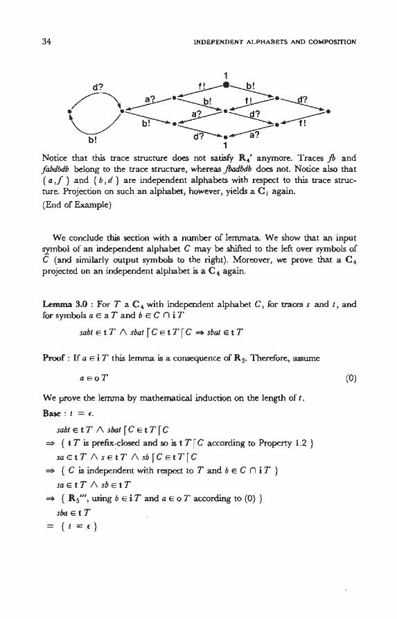
34 INDEPENDENT ALPHABETS AND COMPOSITION

1

d? __.!1---·~ /\ ~-~ _JJ----·~ . -~~-~~· ~ b. -~~· t.

b ' d? • a? . 1

Notice that this trace structure does not satisfy R 4' anymore. Traces Jb and fabdbdb belong to the trace structure, whereas Jbadbdb does not. Notice also that { a ,j } and { b , d } are independent alphabets with respect to this trace struc­ture. Projection on such an alphabet, however, yields a C 1 again.

(End of Example)

We conclude this section with a nwnber of lemmata. We show that an input s_ymbol of an independent alphabet C may he shifted to the left over symbols of C (and similarly output symbols to the right). Moreover, we prove that a C 4

projeeteel on an independent alphabet is a c4 again.

Lemma 3.0 : For T a C 4 with independent alphabet C, for traces s and t, and for symbols a E aT and b E C n i T

sabt E t T (\ sbat f C E t T f C ~ sbat E t T

Proof: If a Ei T this lemma is a consequence of R 3. Therefore, asswne

aEoT

We prove the lemma by mathematical induction on the length of t.

Base : t = f.

sabt E t T (\ sbat f C E t T f C

~ { t T is prefix~closed and so is t T f C according to Property 1.2 }

sa E t T (\ s E t T 1\ sb f C E t T f C

==> { C is independent with respect to T and b E C n i T }

sa E t T 1\ sb E t T

==> { R 5"', using b EiTand a E o T according to (0) }

sba Et T

= {t=f}

(0)

3000 INDEPENDENT ALPHABETS

sbat Et T

Step : t = t0e 0 Assume the left-hand side of the implicationo Hence,

sabt E t T and sbat r c E t T r c

Then we derive

true

= { ( 1 ), using t = toe and the prefix-closedness of t T and t T f C }

sabto E t T 1\ sbato f C E t T f C

==> { induction hypothesis }

sbat 0 etT

35

(1)

(2)

Next, we distinguish three cases : (i) e e o T, (ii) e e C n i T, and (iii) e E i T \ C 0 We prove that sbat oe E t T which yields the result desired, since t = t0e 0

(i) e E o T

true

= { (1) and (2), using t = t 0e }

sabt0e Et T 1\ sbat 0 e t T

==> { R 4", since b Ei T, a E o T according to (0), and e E o T }

sbat0e Et T

(ii) e E C n i T

true

= { (1) and (2), using t = t 0e }

sbat oe f C E t T f C 1\ sbat o E t T

==> { C is independent with respect to T and e E C n i T }

sbat0e Et T

(iii) e E i T \ c true

= { ( 1 ), using t = t 0e and projection on a T \ C, and (2) }

sabt 0e f(a T \ C)e t T f(a T\ C) 1\ sbat0 e t T

36 INDEPENDENT ALPHADETS AND COMPOSITION

{ distribution of projection over concatenation, using b E C }

sbat0c r(a T \ C)e t rr(a T\ C) 1\ sbat0 e t T

~ { a T \ C is independent with respect to T, since C is, and c E (aT\ C) n i T }

sbat0c Et T

(End of Proof)

Lemma 3.1 : For T a C 4 with independent alphabet C, f()r traces s, t, and u, and for symbol a E c n i T such that t re = E

stau E t T ~ satu E t T

Proof : By mathematica! induction on the length of t.

Base : t = t:. Obvious.

Step : t = t0b. Hence, we have

tor C = E and b fl C

stau Et T

= { t = t0b and projection on C }

stobau E t T 1\ stobau r C E t T r C

= { distribution of projection over concatenation, using b fl C according to (0) }

stobau E t T 1\ stoabu r C E t T r C

~ { Lemma 3.0, since a E C n i T }

stoabu Et T

~ { induction hypothesis, using (0) }

sat0bu Et T

= { t = t0b }

satu Et T

(End of Proof)

In a similar way, using that aT \ C is independent as well, we derive

(0)

3.0. INDEPENDENT ALPHABETS 37

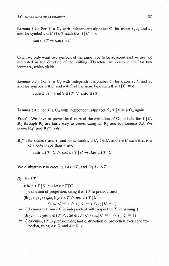
Lemma 3.2 : For T a C 4 with independent alphabet C, for traces s, t, and u, and for symbol a E c n 0 T such that t re = t:

satu E t T ~ stau E t T

Often we only want two symbols of the same type to he adjacent and we are not interested in the direction of the shifting. Therefore, we combine the last two lemmata, which yields

Lemma 3.3 : For T a C 4 with independent alphabet C, for traces s, t, and u, and for symbols a E C and b E C of the same type such that t r C = t:

satbu E t T ~ sabtu E t T V stabu E t T

Lemma 3.4 : For T a C 4 with independent alphabet C, T f C is a C 4 again.

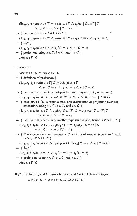
Proof : We have to prove the 6 rules of the definition of C 4 to hold for T f C. R 0 through R 3 are fairly easy to prove, using for R 2 and R 3 Lemma 3.3. We prove R 4" and R 5"' only.

R 4" : for traces s and t, and for symbols a E C, b E C, and c E C such that b 1s of another type than a and c

sabtc E t T f C 1\ sbat E t T f C ~ sbatc E t T f C

We distinguish two cases : (i) bEi T, and (ii) bEo T

(i) bEi T

sabtc E t T f C 1\ sbat E t T f C

= { definition of projection, using that t T is prefix-closed }

(3s 0 'sI 's 2 : : s oasIbs 2c E t T 1\ sbat E t T r c 1\ s0 fC = s 1\ s 1 fC = t: 1\ s2 fC = t)

~ { Lemma 3.1, since C is independent with respect to T, renaming }

(3s o , s 1 : : s oabs 1 c E t T 1\ sbat E t T f C 1\ s o f C = s 1\ s 1 f C = t )

{ calculus, t T is prefix-closed, and distribution of projection over concate­nation, using a E C and b E C }

38 INDEPENDENT ALPHABETS AND COMPOSITION

(3s 0 'sI : : s oabs I c E t T 1\ s oabs I E t T 1\ J obas I re E t T re

1\ sore = s /\si re = t)

=> { Lemma 3.0, since b E e n i T }

(3s 0 'sI : : s oabs I c E t T 1\ s obas I E t T 1\ s 0 re = s 1\ sI re = t)

=> { R4" }

(3s 0 's I : : s obas I c E t T 1\ s 0 r e = s 1\ s I r e = t)

=> { projection, using a E e, b E e, and c E e } sbatc Et Tre

(ii) bEo T

sabtc E t T re 1\ sbat E t T re

= { definition of projection }

(3so ,si ,s2:: sabtc Et T re 1\ sobslas2E t T

1\ sore = s 1\ slre = t: 1\ s2re = t)

=> { Lemma 3.2, since e is independent with respect to T, renaming }

(3s o , s 1 : : s obas 1 E t T 1\ sabtc E t T re 1\ s o re = s 1\ s 1 re = t)

= { calculus, t T re is prefix-closed, and distribution of projection over con­catenation, using a E e, b E e, and c E e }

(3s o , s 1 : : s obas 1 E t T 1\ s oabs 1 re E t T r e 1\ s oabs 1 c r e E t T re

1\ sore = s 1\ s, re = t)

=> { Lemma 3.0, since a is of another type than b and, hence, a E e n i T }

(3so ,si:: sobas, Et T 1\ soabsl Et T 1\ soabslc reEt T re

l\s0 re =s /\s1 re = t)

=> { e is independent with respect to T and c is of another type than b and, hence, c E e n i T }

(3so ,si:: sobasl Et T 1\ soabslc Et T 1\ So re = s 1\ SI re = t)

=> { R/'}

(3s 0 'sI : : s obas I c E t T 1\ s 0 re = s 1\ sI re = t)

=> { projection, tising a E e, b E e, and c E e } sbatc Et Tre

R 5"' : for trace s, and for symbols a E e and b E e of different types

sa E t T re 1\ sb E t T re => sab E t T re

3.1. COMPOSffiON

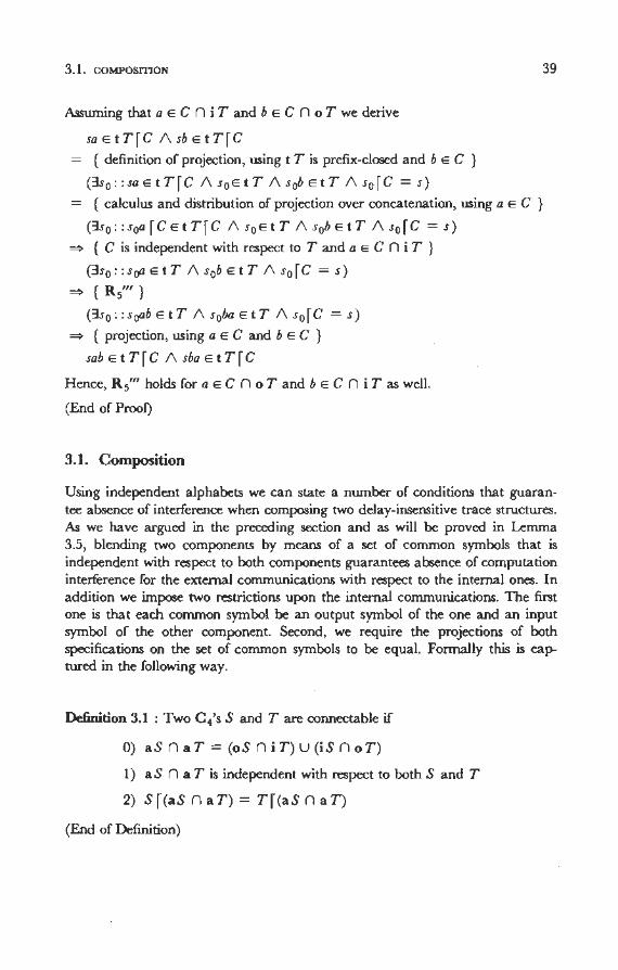
Assuming that a E c n i T and b E c n 0 T we derive

sa E t T r C (\ sb E t T r C

= { definition of projection, using t T is prefix-closed and b E C }

(3so: :sa Et T r C 1\ sa Et T 1\ sab Et T 1\ sar C = s)

= { calculus and distribution of projection over concatenation, using a E C }

(3so: :soa rcEtTrc (\ SoEtT (\ sab EtT (\ sarc = s)

~ { C is independent with respect to T and a E C n i T }

(3so:: soa Et T 1\ sab Et T 1\ sar C = s)

~ { Rs"' }

(3s 0 ::s0ahEtT l\ s0haEtT l\s0 rc =s)

~ { projection, using a E C and b E C }

sab E t T r C (\ sba E t T r C

Hence, Rs"' holelsfora E c n 0 Tand b E c n i Tas well.

(End of Proof)

3.1. Composition

39

Using independent alphabets we can state a number of conditions that guaran­tee absence of interterenee when composing two delay-insensitive trace structures. As we have argued in the preceding section and as will be proved in Lemma 3.5, blending two components by means of a set of common symbols that is independent with respect to both components guarantees absence of computation interterenee for the extemal communications with respect to the intemal ones. In addition we impose two restrictions upon the internal communications. The first one is that each common symbol be an output symbol of the one and an input symbol of the other component. Second, we require the projections of both specifications on the set of common symbols to be equal. Formally this is cap­tured in the following way.

Definition 3.1 : Two C/s S and T are connectable if

O) aS n a T = (oS n i T) u (is n o T)

1) aS n a T is independent with respect to both S and T

2) S r(aS naT)= rr(aS naT)

(End of Definition)

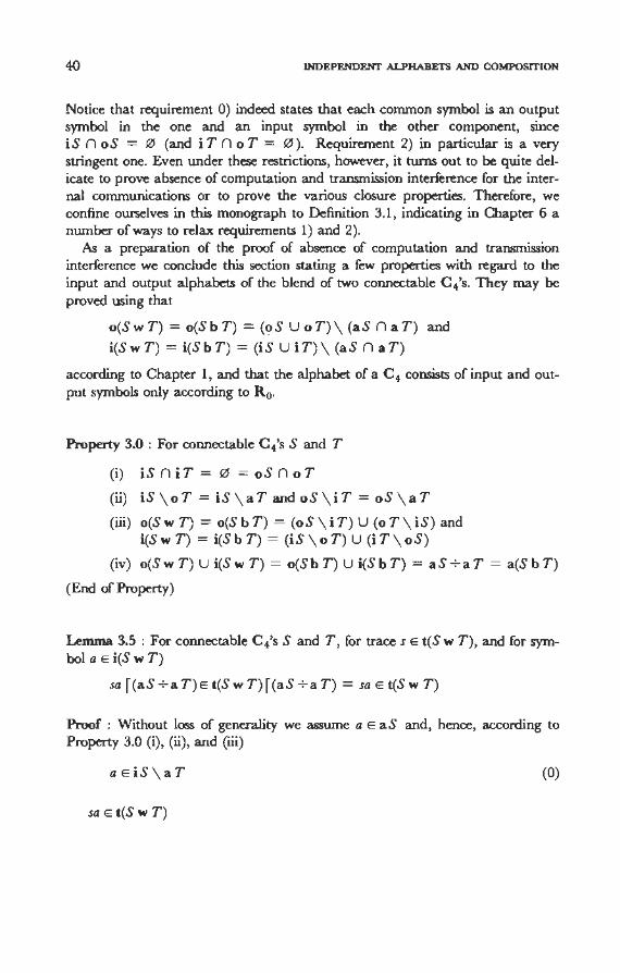
40 INDEPENDENT ALPHABETS AND COMPOSITION

Notice that requirement 0) indeed states that each common symbol is an output symbol in the one and an input symbol in the other component, since iS n oS = 0 ( and i T n o T = 0 ). Requirement 2) in particwar is a very stringent one. Even under these restrictions, however, it turns out to be quite del­icate to prove absence of computation and transmission interference for the inter­na! communications or to prove the various ciosure properties. Therefore, we confine ourselves in this monograph to Definition 3.1, indicating in Chapter 6 a number of ways to relax requirements 1) and 2).

As a preparation of the proof of absence of computation and transmission interference we conclude this section stating a few properties with regard to the input and output alphabets of the blend of two connectable C 4's. They may be proved using that

o(S w T) = o(S b T) = ('?S U o T) \(aS naT) and

i(SwT) = i(SbT) =(iS UiT)\ (aS naT)

according to Chapter 1, and that the alphabet of a C 4 consists of input and out­put symbols only according to R 0.

Property 3.0 : For connectable C 4's S and T

(i) iS n i T = 0 =oS n o T

(ii) iS \ o T = iS \ aT and oS \ i T = oS \ aT

(iii) o(SwT) = o(SbT) = (oS \ iT) U (oT \ iS) and i(SwT) = i(SbT) = (iS\oT) U (iT\oS)

(iv) o(SwT) U i(SwT) = o(SbT) U i(SbT) = aS --7-- aT = a(SbT)

(End of Property)

Lemma 3.5 : For connectable C 4's S and T, fortraces E t(S w T), and for sym­bol a E i(S w T)

sa r(aS--7--a T)e t(Sw T)r(aS7a T) =sa e t(Sw T)

Proof : Without loss of generality we assume a E aS and, hence, according to Property 3.0 (i), (ii), and (iii)

aeiS\aT (0)

sa E t(S w T)

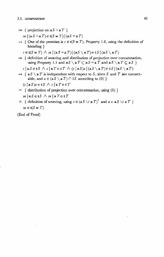
3.1. COMPOSITION

==> { projection on aS +a T }

sa r (as +a T) E t( s w TH (as +a T)

==> { One of the premises is s E t(S w T). Property 1.8, using the definition of blending}

s E t( s w T) (\ sa r (as +a TH (as \ a T) E t s r (as \ a T)

==> { definition of weaving and distri bution of projection over concatenation, using Property 1.1 and aS \ a T !;;; aS +a T and aS \ a T ç;; aS }

s ra S E t S 1\ s ra T E t T 1\ ( s ra S )a r (aS \ a T) E t S r (aS \ a T)

==> { aS \ aT is independent with respect to S, since S and T are connect­able, and a E (aS \a T) n iS according to (0) }

(sras)aetS 1\ sraTetT

= { distribution of projection over concatenation, using (0) }

sa raS E t S 1\ sa ra TE t T

= { definition ofweaving, using sE (aS U a T)• and a E aS U aT }

sa E t(S w T)

(End of Proof)

41

4

Internal communications and external specification

The main issue of this chapter is to show absence of transmission and computa­tion interference under composition of connectable C 4's. Since interference is a physical notion for mechanisms that send and receive signals, we begin this chapter with the introduetion of a mechanistic appreciation of composition. In the last section it is argued that the blend is an operator for the specification of the composite that is in accordance with this mechanistic appreciation.

4.0. An informal mechanistic appreciation

We consider a mechanism and its environment that communicate with one another by sending and receiving signals. There are two types of signals : from the environment to the mechanism, the so-called inputs, and from the mechan­ism to the environment, which we call outputs. We assume that signals are con­veyed via (finitely many) wires. With each wire we associate a syrnbol. A signal via a wire is denoted by its associated syrnbol.

A trace structure . is viewed as the specification of such a mechanism­environment pair .. Each syrnbol of the trace structure's alphabet corresponds to one wire. The alphabet is partitioned into an input and an output alphabet.

A trace is conceived as a sequence of events. Due to the concurrency of signals and the dependency of observations upon the position, there might not exist a unique sequence of events that describes the history of a mechanism-environment pair in operation. This history is rather described, at any time during operation, by a set, or equivalence class, of sequences of events. Traces that differ from one another because of the concurrency of syrnbols belong to the same equivalence class. Yet we associate, at any time during operation, one single trace, being a

4.0. AN INFORMAL MECHANISTIC APPRECIATION 43

sequence of events, with the operation of a mechanism-environment pair. This trace is called the trace thus · far generated. Since the discussion in the sequel relates to an arbitrary trace thus far generated it pertains, in fact, to the equivalence class of sequences of events.

Initially, the trace thus far generated is €. The operation of the mechanism­environment pair corresponds to the generation of symbols. Each signal that the mechanism and environment communicate with one another can be viewed as the extension of the trace thus far generated with the symbol that is associated with that signal. Notice that only those extensions are allowed that yield a trace that belongs to the trace structure again.

We say that output symbols in the trace thus far generated have been sent and input symbols have been received by the mechanism. Whenever more con­venient, we say that these symbols have been sent or received by the trace thus far generated instead of by the mechanism.

Under composition of two mechanism, wires to which the same symbol corresponds are connected. A wire that conveys input signals to the one mechan­ism should convey output signals from the, other one. Accordingly, under compo­sition of two trace structures, a common symbol is an input symbol of the one and an output symbol of the other trace structure. Composition can be viewed as replacing (a part of) one mechanism's environment by the other mechanism­environment pair.

We assume the so-called causality rule for mechanisms, i.e. no input signal can be received before the corresponding output signal has been sent. For the mechanistic appreciation of composition this means the following. At any instant, there are two traces thus far generated, one for each of the mechanism­environment pairs. Each trace ,may be extended with a symbol in the way described above, under the additional restrietion that for each common symbol the number of times it has been received by the one trace does not exceed the number of times it has been sent by the other one.

A symbol sent by the one trace that has not been received by the o~er .one is said to be on its way. Any two traces that can be brought a bout observing , the restrictions above are called composable.

Absence of transmission and computation interterenee can be expressed in terrns of composable traces. There is absence of transmission interterenee if we have for all pairs of composable traces : the number of occurrences of a common symbol sent by the one trace exceeds the number of occurrences of that symbol received by the other trace by at most one. There is absence of computation interterenee if we have for all pairs of composable traces : a symbol on its way from one trace to the other can be received by the latter, i.e. the extension of the latter trace with this symbol belongs to the trace structure of the corresponding mechanism.

We prove in the next sections that there is absence of computation and transmission interterenee under composition of two connectable C 4's. Therefore,

44 INTERNAL COMMUNICATIONS AND EXTERNAL SPECIFICATION

we believe that the formal properties of delay-insensitivity and connectability provide a model that can he usefully applied to the problem of composing physi­cal circuits and deriving the specification for the resulting circuit from the specifications of the composing circuits.

4.1. Formalization of the mechanistic appreciation

In this section we formalize the mechanistic appreciation as introduced above and the proof obligations for showing absence of transmission and computation interference.

Definition 4.0 : For connectable trace structures T and U, the composability of traces t E t T and u E t U, denoted by c ( t , u), is defined by

t=(/\u=(V

(3a,t0 ::t =toa /\c(t 0 ,u)/\(aEoU=>#au>#ato)) V

(3b,u0 : : u = u0b 1\ c(t,u0) 1\ (bEo T => #bt >#buo))

(End of Definition)

Notice that c(t,u) = c(u,t). Notice also that a E oU and t =toa implies a E a T n a U and, hence, on account of the definition of connectability, a E i T.

To cope with the various appearances of the arguments of c we state the fol­lowing properties, which can readily he derived from the definition of c . When referring to the definition of c , one of the following properties may he meant.

Property 4.0 :

(i) c(ta,ub) = c(t,ub) 1\ (a E oU => #aub >#at) V c(ta,u) 1\ (b E oT => #bta >#hu)

(ii) c(ta,u) = c(t,u) 1\ (a EoU =>#au >#at) V (3b,u0 ::u = u0b 1\ c(ta,u0) 1\

(bEo T => #bta >#buo))

(iü) c(t,()=(trou=()

(End of Property)

The two theorems that we have to prove are

4.1. FORMALIZATION OF THE MECHANISTIC APPRECIATION 45

Theorem 4.0 : (Absence of transmission interference) For connectable C 4's T and U, for composable traces t E t T ~d u E t U, and for symbol a E o T n i U

#at -#au~ 1

Theorem 4.1 : (Absence of computation interference) For connectable C 4's T and U, for composable traces t E t T and u E t U, and for symbol a E o T n i U

such that #at >#au : ua E tU.

These two theorems are proved in the next section. We conclude this section with a few lemmata on composable traces.

Lemma 4.0: For connectable C 4's Tand U, fortraces t and u, and for symbol a such that ta E t T and u E t U

c(ta,u) 1\ a f1. i U==> c(t,u)

Proof : By mathematica! induction on the length of u .

Base: u = t:. c(ta , u) 1\ afl.iU

==>{u =t:}

c(ta,t:)

= { definition of c }

c (t' t:) = {u=t:}

c(t,u)

Step : u = u0b. Now we derive

c(ta,u) 1\.afl.iU

= {u = uoh } c(ta,u0b) 1\ a fl.iU

= { definition of c and calculus }

c(t ,uoh) 1\ (a E o U==> #au 0b >#at) 1\. a f1. i U V

c(ta,u0) 1\ (beoT==>#bta>#buo) 1\.afl.iU

==> { calculus, using u = u0b, and the induction hypothesis }

c (t, u) V c (t, u0 ) 1\ (b E o T ==> #b ta >#buo) 1\ a f1. i U

46 INTERNAL COMMUNICATIONS AND EXTERNAL SPECIFICATION

~ { calculus, using that b E a U and b E o T implies, by the connectability of T and U, b E i U }

c(t,u) V c(t,u0) 1\ b fl o T V c(t,u0 ) 1\ #bta >#buo 1\ a =I= b

~ { definition of c, using u = u0b , and calculus }

c(t,u) V c(t,uo) 1\ #bt >#buo

~ { definition of c, using u = u0b }

c(t,u)

(End of Proof)

Lemma 4.1 : For connectable C 4's Tand U, fortraces t and u, and for symbol a such that ta E t T and u E t U

c(ta,u) 1\ #ata >#au ~ c(t,u)

Proof : By mathematica! induction on the length of u .

Base: u = t:.

c(ta,u) 1\ #ata >#au

={u =t:}

c(ta,t:)

~ { definition of c }

c (t, t:)

= { u = ( } c (t, u)

Step : u = u0b. Now we derive

c(ta,u) 1\ #ata >#au

= {u = u0b }

c(ta,u0b) 1\ #ata >#auob

= { definition ofc and calculus }

c(t,uob) 1\ (a E oU ~ #auob >#at) 1\ #ata >#auob V

c(ta,u0) 1\ (bEo T ~ #bta >#buo) 1\ #ata >#au0b

~ {calculus, using u = u0b }

c(t,u) V

c(ta,uo) 1\ (bEo T ~ #bta >#buo) 1\ #ata >#au0b 1\ a = b V

c(ta,uo) 1\ (bEo T ~ #bta >#buo) 1\ #ata >#auob 1\ a =I= b

4.1. FORMALIZATION OF THE MECHANISTIC APPRECIATION

=> { calculus }

c(t,u) V c(ta,u 0) 1\ #at >#auo 1\ a = b V

c(ta,uo) 1\ (b E oT => #ht >#buo) 1\ #ata >#auo

=> { induction hypothesis and calculus }

c(t,u) V c(t,u0) 1\ #ht >#buo V c(t,u0) 1\ (bEo T => #ht >#buo)

=> { defirution of c, using u = u0b }

c(t,u)

(End of Proof)

47

Lemma 4.2 : For connectable C4s Tand U, fortraces tE t Tand u Et U, and for symbol a E a T n a U

c(t,u)/\#at>#au =>aEoTniU

Proof : By mathematica! induction on I t + I u.

Base: lt +Iu = 0. Then #at =#au.

Step: lt + Iu = k, forsome k, k;;;;;.: 1. Now we derive

C ( t, U) 1\ #at >#a U

= { definition of c, using •(t = f 1\ u = f) since k ;;;;;.: 1. Calculus }

(3b,to::t =tob 1\ c(to,u) 1\ (b EoU =>#hu >#hto) 1\ #at0b >#au) V

(3b,u0 : :u = u0b 1\ c(t,u0) 1\ (b EoT => # 6 t >#6u0) 1\ #at >#au0b)

=> { Induction hypothesis applied to the second disjunct. Calculus }

(3b,to::b =a l\(bEoU=>#hu>#ht0)/\#atob>#au) V

(3 b , t o : : b =/= a 1\ c ( t o , u ) 1\ #a t 0b > #a u ) V a E o T n i U

=> { lnduction hypothesis applied to the second disjunct. Calculus }

(3to: :(a E 0 u => #a u >#a to) 1\ #a to;;;;;.: #a u) V a E 0 T n i u => { calculus, using a E a T n a U and the connectability of T and U on

account of which a fi o U = a E o T n i U }

aEoTniU

(End of Proof)

From Lenuna 4.2 we infer the following corollary, using the synunetry of c and (o T n i U) n (o UniT) = 0. ·

48 INTERNAL COMMUNICATIONS AND EXTERNAL SPECIFICATION

Corollary 4.0 : For connectable C 4's T and U, for traces te t T and u et U, and for symbol a e a T n a U

c(t,u) 1\aeoTniU~#at~#au

4.2. Absence of transmission and computation interference

(This section may be skipped on first reading.) In this section we prove the absence of transmission and computation interference. To that end we consider, for connectable trace structures T and U and for composable traces t e t T and u e t U, symbols on their way from one trace to the other. Rather than consicl­ering these symbols individually, we consider the set of sequences of symbo.ls, called traces again, consisring of the symbols on their way in one direction.

Definition 4.1 : For connectable trace structures Tand U, and for composable traces t e t T and u e t U we de fine from ( t , u ) as

{ x : x e ( o T n i U)" 1\ ('f/ a : a E o T n i U : #a x = #at -#a 14) : x }

(End of Definition)

Consequently, from ( t, u ) is the set of traces that are a permutation of all sym­bols sent by t and not received by u. Since #at ~#a u for a e o T n i U on account ofCorollary 4.0, from(t,u) is non-empty. Since the lengths ofthe traces in from ( t , u) are equal, we define I (from ( t, u)) as the length of the traces in from (t, u), which is the number of symbols on their way from t to u.

The total number of symbols on their way between t and u is called the number of mismatches and is denoted by nun (t, u).

Definition 4.2 : For connectable trace structures T and U, and for composable traces t e t T and u e t U

nun(t,u) = l(from(t,u))+l(from(u,t))

(End of Definition)

We shall frequently use the following properties of from and mm. Proofs are omitted but can be derived using the definitions and Lemmata 4.0 and 4.2.

4.2. ABSENCE OF TRANSMISSION AND COMPUTATION INTERFERENCE 49

Property 4.1 : For connectable trace structures T and U, and for composable tracestEtTanduEtU

(i) u0 Efrom(t,u) 1\ uu0 EtU ~c(t,uu0)

(ii) u0 E from(t,u) 1\ uu 0 E tU ~ from(t,uu 0) = { t:}

(iii) u= u0u 1 1\ u 1 EoT* ~mm(t,u0) = mm(t,u0u 1)+lu 1

(iv) u= u0u1 1\ u1 EoT* 1\ u2 Efrom(t,u0u 1) ~u 1u 2 Efrom(t,u0)

(v) u = UoUl 1\ u, riT= ( ~ from(uoUl ,t) = from(uo,t)

(End of Property)

In order to prove Theorems 4.0 and 4.1, the absence oftransmission· and compu­tation interference respectively, we prove the following lemma.

Lemma 4.3 : For connectable trace structures T and U such that a T = a U, and for composable traces t E t T and u E t U

(\fu 0 : u0 E from (t, u): uu 0 Et U)

Theorems 4.0 and 4.1 are derived from this lemma in the following way. Let T and U he connectable C 4's and let tE t T and u Et U he corriposable traces. Since a T n a U is independent with respect to both T and U, T r (a T n a U) and U r (aT n a U) are C 4's as well according to Lemma 3.4. Moreover, their alpbahets are equal, viz. a T n a U, and they are connectable as follows from the definition of connectability.

From the definition of composability it can he seen that the strings of common symbols in t and u determine both the composability of t and u and the sym­bols on their way from t to u. Hence, from the composability of t and u with respect to T and U we infer the composability of t r (a T n a U) and u r(a T na U) with respecttoT r(a T na U) and ur(a T na U). Let u0 he a string of all symbols on their way from t to u. Then u0 is a string of all symbols on their way from t r (a T n a U) to u r (a T n a U) as well. This implies that (u r(a T na U))u 0 E t U r(a T na U) according to Lemma 4.3. The symbols of u0 are input symbols to U and helong to aT na U. Since aT na U is independent with respect to U and since u E t U we conclude, by applying Definition 3.0 a number of times, that uu0 E t U.

50 INTERNAL COMMUNICATIONS AND EXTERNAL SPECIFICATION

Notice that u0 is an arbitrary permutation of the symbols on their way from T to U, i.e. of symbols a E o T ()i U with # 0 t >#0 u. First, uu0E t U then implies that each symbol occurs at most once in u0, since, on account of R 2,

adjacent symbols are distinct. Hence, we have proved absence of transmission interference. Second, again since u0 is an arbitrary permutation of symbols on their way and, hence, may start with any symbol on its way from t to u , it implies absence of computation interference, since t U is prefix-closed.

Lemma 4.3 is proved by mathematica! induction. In order to reduce the length of the proof we first prove two additional lemmata, in which we assume the induction hypothesis for Lemma 4.3. Let, for the remainder of this section T and U be connectable C 4's such that aT= aU. Consequently, i T = oU, oT =i U, and tT = tU.

Lemma 4.4 : Given integer k and given that all composable traces t E t T and u Et U with Jt +Iu +mm(t,u)~k satisfy

('v'u0 :u0Efrom(t,u):uu0E tU) 1\ ('v't0 :t0E from(u,t):tt0EtT)

Then for traces s, t ' u ' V , and w ' and for symbol a E 0 T such that t E 0 u·' v E. o T• , satw E t T, and uavw E t U

c (satw, uavw) 1\ 1 (satw) + 1 (uavw) + mm (satw, uavw) ~ k

~ stawEt T 1\ uvawEt U 1\ c(staw,uvaw)

Proof : By mathematica! induction on the length of w.

Base : w = t:. We assume the left-hand side of the implication, hence,

c (sat, uav) and 1 (sat) + 1 (uav) + mm (sat, uav) ~ k

Let t 0 and u0 be such that

t0 E from(uav,sat) and u0 E from(sat,uav)

(0)

(1)

Since t T is prefix-closed, and since a and the symbols of v are of the same type, which makes R3 applicable, we have

saEtT and uva E tU (2)

Now we derive

true

= {(O)and(l)}

c(sat ,uav) 1\ l(sat)+I(uav)+mm(sat,uav)~k 1\

4.2. ABSENCE OF TRANSMISSION AND COMPUTATION INTERFERENCE

t0 E from (uav, sat) 1\ u0 E from (sat, uav)

~ { Lemma 4.0, Property 4.1 (üi), (iv), and (v), using tE o u• } c (sa, uav) 1\ l (sa)+ l (uav) + mm (sa, uav) ~ k 1\

tt0 E from (uav, sa) 1\ u0 E from (sa, uav)

~ { Lemma 4.0, Corollary 4.0, and Property 4.1 (üi), (iv), and (v), using avEoT*}

c(sa,u) 1\ #asa >#au 1\ I(sa)+Iu +mm(sa,u)~k 1\

tt0 E from(u,sa) 1\ avu 0 E from(sa,u)

~ { Lemma 4.1, definition of mm and from, using a E o T }

51

c(s,u) 1\ Is +Iu +mm(s,u)",;;;k-2 1\ tt0 Efrom(u,s) 1\ vu0 Efrom(s,u)

~ { premise}

stt 0 EtT 1\ uvu0 EtU 1\ c(s,u) 1\ tt0 Efrom(u,s) 1\ vu0 Efrom(s,u)

~ { Property4.1 (i)and(v),usingtt0EoU* andvu0EoT*}

stt 0 Et T 1\ uvu0 Et U 1\ c (stt 0 , uvu 0)

~ { t T and t u are prefix-closed, Lemma 4.0, using toE 0 u· and Uo E 0 r· } st E t T 1\ uv E t U 1\ c (st , uv )

~ { Lemma 2.2, using (2) and the fact that a and the symbols of t are of different types }

sta Et T 1\ uva Et U 1\ c (st, uv)

~ { definition of c, using #ast ~#a uv according to Corollary 4.0 }

sta Et T 1\ uva Et U 1\ c (sta, uva)

= {w=t:}

staw E t T 1\ uvaw E t U 1\ c ( staw, uvaw)

Step : w = w 0c. Assuming the left-hand side of the implication again, we have

c (satw0c, uavw 0~) and

l (satw 0c) + l (uavw 0c) + mm (satw 0c, uavw0c) ",;;;;; k

Now we derive

true

= { (3) }

satw0c E t T 1\ uavw0c E t U 1\ c (satw 0c, uavw0c) 1\

I(satw0c) + l (uavwoe) + mm(satw0c ,uavw0c) ~ k

~ { Lemmata 4.0 and 4.1, Corollary 4.0, and the definition of mm }

satwoc E t T 1\ uavwoe E t u 1\ c (satwo 'uavwo) 1\

(3)

52 INTERNAL COMMUNICATIONS AND EXTERNAL SPECIFICATION

I (satw 0) +I (uavw 0) + mm(satw0, uavw0) ~ k -2

~ { induction hypothesis and the deficition of rnm. Moreover, a and the sym­bols of v are of the same type, which makes R 3 applicable }

satw0c Et T 1\ staw0 Et T 1\ uvaw0c Et U 1\ c (staw0 , uvaw0) 1\

I (staw 0) + l(uvaw0) + mm(staw0 ,uvaw0) ~ k -2 (4)

We distinguish two cases : (i) c E o T and (ü) c E o U

(i) c E o T

true

= { (4), applying Lemma 2.6, using that the symbols of t are of another type than a and c ; calculus }

staw0c Et T 1\ uvaw0c Et U 1\ c (staw0, uvaw0)

~ { deficition of c, using #, staw0 ~ #, uvaw0 according to Corollary 4.0 }

staw0c Et T 1\ uvaw0c Et U 1\ c (staw0c, uvaw0c)

= { WoC = W }

staw E t T 1\ uvaw E t U 1\ c (staw, uvaw)

(ii) c E 0 U

true

= { ( 4) and calculus }

stawo E t T 1\ uvawoe E t u 1\ c (stawo' uvawo) 1\

I (stawo) +I (uvawo) + mm(stawo, uvaw0) ~ k- 2 ~ { deficition of c and rnm, using c E o U and #, uvaw0 ~ #,staw0 according

to Corollary 4.0 }

staw0 Et T 1\ uvaw0c Et U 1\ c (staw0 , uvaw0c) 1\ #,uvawoe > #,staw0 1\

I (staw0) +I (uvaw0c) + mm(staw0, uvaw0c) ~k

~ { premise, using that t T is prefix-closed and that there is a trace in from(uvaw 0c ,staw0) that begins with c }

staw0c Et T 1\ uvaw0c Et U 1\ c (staw0 , uvaw0c) 1\ #, uvaw0c > #,staw0 ~ { deficition of c , using c E o U }

staw0c Et T 1\ uvaw0c Et U 1\ c (staw0c, uvaw0c)

= { W = WoC }

stawEt T 1\ uvawEt U 1\ c(staw ,uvaw)

4.2. ABSENCE OF TRANSMISSION AND COMPUTATION INTERFERENCE 53

(End of Proof)

Lemma 4.5 : Given integer k and given that all composable traces t E t T and u E t U with I t +I u + mm ( t, u) os;;; k satisfy

(Vu0 : u0 E from(t ,u): uu0 Et U) 1\ (Vt0 : t0 E from(u, t): tt0 E t T)

Then for composable traces t E t T and u E t U with I t + I u = k - 1 and mm(t,u) = 0

(Vc : c E o T: te Et T ~ uc Et U) 1\ (Vc : c E o U : uc Et U ~ teE t T)

Proof : We observe, since aT = a U, that the lengtbs of composable traces

t E t T and u E t U with mm ( t , u) = 0 are equal. Moreover, if these traces are non-empty, at least one of them contains a symbol that is an output symbol for the trace structure to which that trace belongs.

We prove the theorem by mathematical induction on the length of the longest common suffix of t and u.

Base : The length of the longest common suffix of t and u equals I t and I u . Then t = u and the lemma holds, since t T = t U, due to the connectability of Tand U.

Step:

t = t0w and u = UoW with c(t,u), lt + Iu = k -1,

and mm (t, u) = 0 (0)

Traces t 0 and u0 are non-empty and do not end in the same symbol. Notice that we assume the lemma to hold for composable traces with a longest common suffix that is longer than w. Applying Lemmata 4.0 and 4.1, using the definition of from , we derive from (0) and the composability of t and u

(1)

Wedefine r, t2, s, and v in the following way.

to = rl2 and Uo = SV with t2E ou• and V E 0 r• (2)

r and v do not end in a symbol of o U and o T respectively (3)

Moreover we have, according to the observation made at the beginning of this proof

lr+ls>O (4)

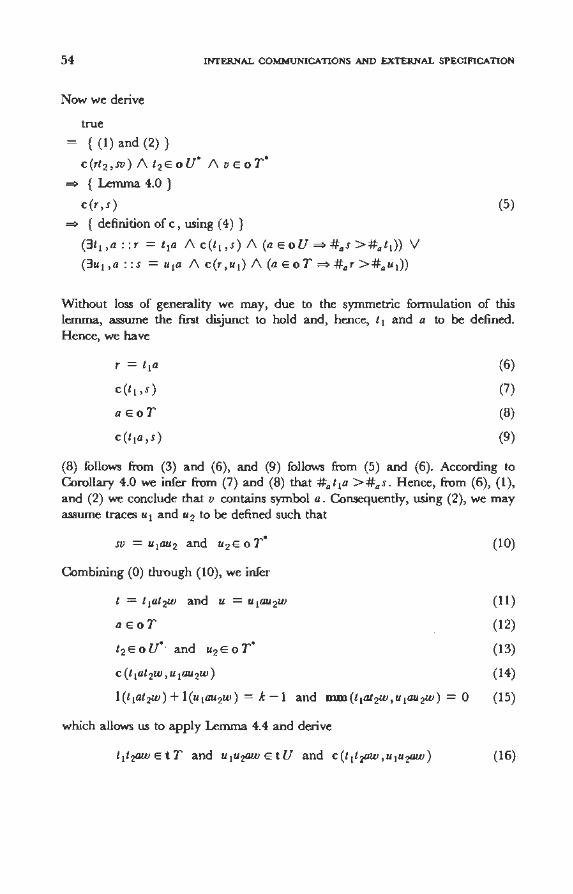
54 INTERNAL COMMUNICATIONS AND EXTERNAL SPECIFICATION

Now we derive

true

= { ( 1) and (2) }

C (rt2, SV) (\ t2 E 0 u• (\ V E 0 r• => { Lemma 4.0 }

c (r, s)

=> { definition of c , using ( 4) }

(3t 1 ,a:: r = t 1a 1\ c(t 1 ,s) 1\ (a E o U=> #as >#at 1)) V

(3u 1 ,a : : s = u 1a 1\ c(r ,u 1) 1\ (a E o T =>#ar >#au 1))

(5)

Without loss of generality we may, due to the symmetrie formulation of this lemma, assume the fust disjunct to hold and, hence, t 1 and a to be defined. Hence, we have

c(t 1 ,s)

aEoT

(6)

(7)

(8)

(9)

(8) follows from (3) and (6), and (9) follows from (5) and (6). According to Corollary 4.0 we infer from (7) and (8) that #at 1a >#as. Hence, from (6), (1), and (2) we conclude that v contains symbol a. Consequently, using (2), we may assume traces u1 and u2 to be defined such that

(10)

Combining (0) through (10), we infer

t = t 1at 2w and u = u1au 2w (11)

a E o T (12)

t 2 EoU· and u2 EoT· (13)

c (t 1at 2w, u 1au 2w) (14)

l(t 1at2w)+l(u 1au2w) = k-1 and mm(t 1at 2w,u 1au2w) = 0 (15)

which allows us to apply Lemma 4.4 and derive

(16)

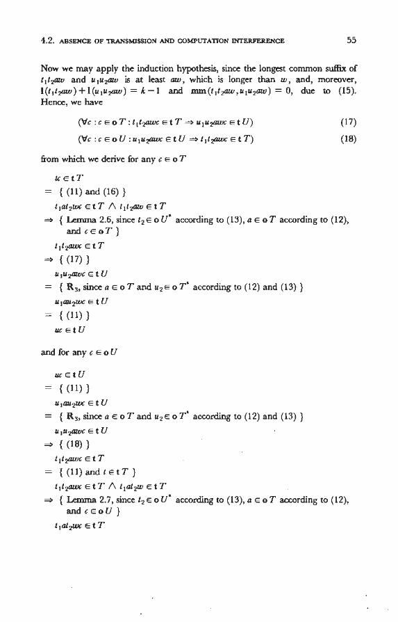
4.2. ABSENCE OF TRANSMISSION AND COMPUTATION INTERFERENCE 55

Now we may apply the induction hypothesis, since the longest corrunon suffix of t 1 t 'l'lW and u 1 u 2'lW is at least aw, which is longer than w, and, moreover, l(t 1t2aw)+l(u 1u2'1W) = k-1 and mm(t 1t2aw,u 1u2aw) = 0, due to (15). Hence, we have

('tic: c E o T: t 1t2awc Et T ~ u 1u2awc Et U)

('tic : c E o U: u1u2'1Wc Et U~ t 1t2awc Et T)

from which we derive for any c E o T

teE t T

= { (11) and (16) }

t 1at 2wc Et T 1\ t 1t2'1W Et T

(17)

(18)

~ { Lerruna 2.6, since t2 E o u• according to (13), a E o T according to (12), andcEoT}

t 1t2awc EtT

~ {(17)}

u1u2awc E tU

= { R3, since a E o Tand u2 E o r• according to (12) and (13) }

u1au 2wc E tU

= { (11)}

uc Et U

and for any c E oU

uc E tU

= {(11)}

u1au 2wc Et U

= { R3, since a E o T and u2 E o r• according to (12) and (13) }

u1u2'1Wc Et U

~ { (18) }

t 1t2awc Et T

= {(11)andtEtT}

t 1t2'1Wc Et T 1\ t 1at 2w Et T

~ { Lemma 2.7, since t2 E o u• according to (13), a E o T according to (12), and cEoU}

t 1at2wc Et T

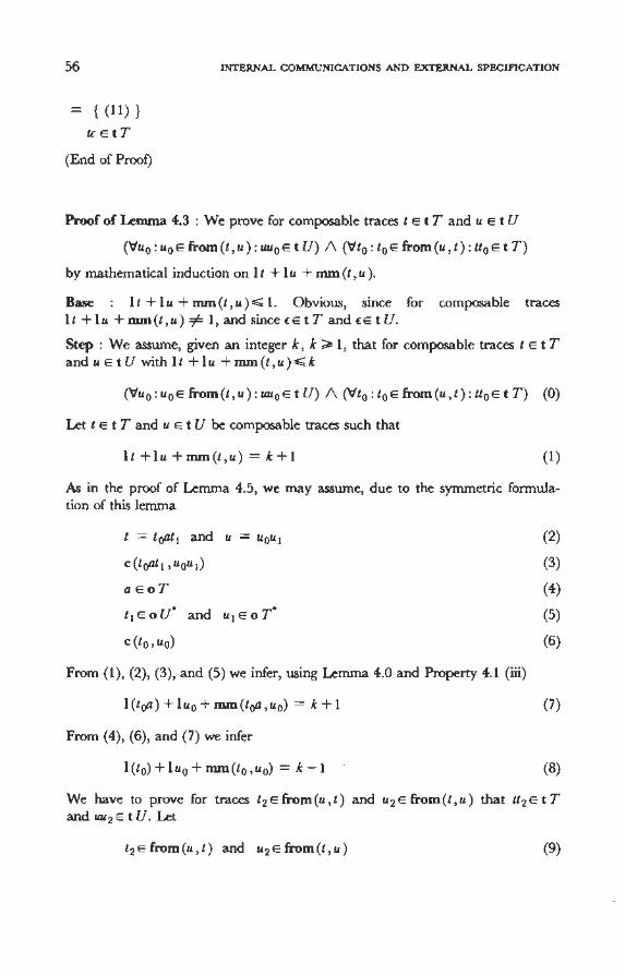
56 INTERNAL COMMUNICATIONS AND EXTERNAL SPECIFICATION

= {(11)}

teE t T

(End of Proof)

Proof of Lemma 4.3 : We prove for composable traces t E t T and u E t U

('v'u0 : u0E from(t,u): uu0E t U) 1\ ('v't0 : t0E from(u,t): tt0E t T)

by mathematica! induction on 1 t + 1 u + mm (t, u).

Base : 1 t + 1 u + mm ( t , u) .;;;:; 1. Obvious, since for composable traces 1 t + 1 u + mm ( t , u) =F 1, and since f. E t T and f. E t U.

Step : We asswne, given an integer k, k ~ 1, that for composable traces tE t T and u Et U with 1 t + 1 u + mm (t, u).;;;:; k

('v'u0 : u0E from(t,u): uu0E t U) 1\ ('v't0 : t0E from(u,t): tt0E t T) (0)

Let t E t T and u E t U be composable traces such that

1t +1u +mm(t,u) = k+1 (1)

As in the proof of Lemma 4.5, we may assume, due to the symmetrie formula­tion of this lemma

e = eoat 1 and U = u0u1

c(toat 1 ,u0u1)

aEoT

t 1 E o u· and UJ E 0 T"

c (to, uo)

From (1), (2), (3), and (5) we infer, using Lemma 4.0 and Property 4.1 (iii)

1(toa)+1u0+mm(t0a,u0) = k+1

From (4), (6), and (7) we infer

1(t0) + 1u0 + mm(t0 ,u0) = k - 1

(2)

(3)

(4)

(5)

(6)

(7)

(8)

We have to prove for traces t2E from(u,t) and u2E from(t,u) that tt2E t T and uu2 E t U. Let

(9)

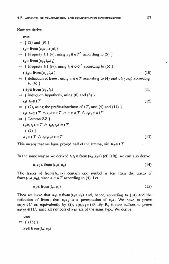
4.2. ABSENCE OF TRANSMISSION AND COMPUfATION INTERFERENCE

Now we derive

true

= { (2) and (9) }

t2 E from(u 0u1 ,toat 1)

=> { Property4.1 (v),usingu 1EoT• accordingto(5)}

t 2 E from(u 0 ,toat 1)

=> { Property4.1 (iv), usingt 1EoU· accordingto (5)}

t 1t 2 E from(u 0 ,toa)

57

(10)

=> { definition offrom, using a E o T according to (4) and c(t0 ,u0) according to (6) }

t 1t 2 E from(u 0 ,t0)

=> { induction hypothesis, using (6) and (8) }

t0t 1t2 EtT

= { (2), using the prefix-closedness oft T, and (4) and (11) }

t0t 1t 2 EtT 1\toaEtT 1\aEoT l\t 1t2 EoU•

=> { Lemma 2.2 }

toat 1t2 EtT 1\ t0t 1t2aEtT

= { (2) }

tt 2 Et T 1\ t0t 1tza Et T

This means that we have proved half of the lemma, viz. tt 2 Et T.

( 11)

(12)

(13)

In the same way as we derived t 1t2 E from(u 0 ,toa) (cf. (10)), we can also derive

(14)

The traces of from ( t0 , u0 ) contain one symbol a less than the traces of from(toa ,u0), since a E o T according to (4). Let

(15)

Then we have that u3a E from(toa,u 0) and, hence, according to (14) and the definition of from, that u1u2 is a permutation of u3a. We have to prove uu 2 EtU or, equivalently by (2), UQU 1u2 EtU. By R 3 it now suffices to prove u0u3a E t U, since all symbols of u3a are of the same type. We derive

true

= { (15)}

u3 E from(t 0 ,u0)

58 INTERNAL COMMUNICATIONS AND EXTERNAL SPECIFICATION

= { induction hypothesis, using (6) and (8) }

u3 E from (t 0 , u0 ) 1\ u0u3 Et U

= { ( 11) and ( 12) }

u3 Efrom(t0 ,u0) 1\ u0u3 EtU 1\ t 1t2 Efrom(u0 ,t0) 1\ t0t 1t2 EtT

~ { Property 4.1 (i), (ii), and (v), using the definition of from }

u0u3 EtU 1\ t 1t2 Efrom(u0u3 ,t0 ) 1\ t0t 1t 2 EtT 1\

from(t 0 ,u0u3 ) = {t:} 1\ u3 EoT• 1\ c(t0 ,u0u3 )

~ { Property 4.1 (i), (ii), and (v), using the definitions of mm and from }

t0t 1t 2 EtT 1\ u0u3 EtU 1\ c(t 0t 1t 2 ,u0u3) 1\ mm(t0th,u0u3) = 01\

u 3 E o T. 1\ tI t 2 E o u· ~ { Lemma 4.5, using l(t0t 1t 2) + l(u0u3) = k -1, which we derive from (8)

and Property 4.1 (iii) }

('Vc :c E oT: t0t 1t2c Et T ~ u0u3c Et U)

~ { instantiation, using a E o T according to (4), and t0t 1t2a Et T according to (13) }

u0u3a Et U

(End of Proof)

4.3. Blending as a composition operator

In the previous section we have proved the absence of transmission and compu­tation interference. In this section we argue that blending as a composition operator is a proper abstraction of the mechanistic appreciation of composition as discussed earlier. We consider this a sufficient justification for using blending as a composition operator for composing C 4's by means of independent alpha­bets.

In the remainder of this section T and U are connectable C 4's. We define for two composable traces the set of resulting traces in the following way.

Definition 4.3 : For traces t Et T, u Et U, and x we say that x is a resultant of tand u, denoted by xr(t,u), if

x = t:/\t = t:/\u=t:V

(3a,x 0 ,t0 ::x =xoa 1\t =toa l\xor(t0 ,u) 1\(aEoU~#au>#ato)) V

(3a,x 0 ,u0 :: x =xoa 1\u =uoa l\xor(t,u0)1\(aEoT~#at>#auo))

(End of Definition)

4.3. BLENDING AS A COMPOSITION OPERATOR 59

Composability of traces t E t T and u E t U equals (3x : : x r ( t, u)). In the remainder of this section the set { x , t , u : t E t T 1\ u E t U 1\ x r ( t , u ) : x } is denoted by S. In view of our mechanistic appreciation it seems reasonable to define the specification of the composite to be S f (aT...;... a U). We shall prove that this specification is equal to Tb U. To that end we observe the following.

Any trace in T w U in which all symbols common to T and U are cloubied belongs to S as can be proved by induction. Therefore, Tb U ç; S f (a T...;... a U). Proving that S f (a T...;... a U) ç; Tb U is more elaborate. At several places it involves induction. We choose for giving an outline of the proof rather than a fully detailed argument, since the latter would in no way contribute to our understanding of the theory developed in this monograph.

Occurrences of symbols in traces are counted from the left starting from 1. Due to the absence of transmission interference, an odd occurrence of a symbol from a T n a U in a trace of S originates from the trace structure where this symbol is an output symbol. In the same way we infer that an even occurrence of a common symbol sterns from the trace structure where this symbol is an input symbol. Therefore, since the origin of non-common symbols is obvious, an x E S can uniquely be unravelled into traces t E t T and u E t U such that xr (t, u). The unravelling can be effectuated by projecting on a composing trace structure's alphabet and omitting the odd occurrences of a common symbol if it is an input symbol for this trace structure, and the even occurrences in case of an output symbol.

We prove that an arbitrary trace x in S can be transformed, without affecting its projection on a T...;... a U, into a trace in T w U. As a consequence, S f (a T...;... a U) is a subset of Tb U, which was the remaining proof obligation. The first step in this transformation is extending x with the common symbols of T and U that occur in x an odd number of times. The resulting trace belongs to S due to the absence of computation interference.

The next step is shifting to the left every even occurrence of a common sym­bol until it is adjacent to the preceding occurrence of that symbol. In the next paragraphs we show that the resulting trace still belongs to S. Assurning this to hold, we first discuss the final step. Due to steps one and two, all common sym­bols occur in pairs. Therefore, the unravelling discussed above is the same as projecting on a composing trace structure's alphabet after having replaced each such pair by a single symbol. Hence, this replacement yields a trace in T w U. In none of the steps have we tampered with the non-common symbols and, hence, S f (aS ...;... a T) is unaffected.

There remains one assumption to be proved, viz. that the trace after shifting still belongs to S. Let x 0bax 1 ES be such that a E aS naT, b E aS U aT, a =fo b, and such that this occurrence of a is even. We prove that xoabx 1 is an element of S as well. By repeatedly applying this interchange for symbols to be shifted to the left it can be seen that our assumption indeed holds. We distin­guish two cases : (i) these occurrences of a and b originate from two distinct

60 INTERNAL COMMUNICATIONS AND EXTERNAL SPECIFICATION

trace structures, and (ii) they originate from the same trace structure.

(i) Without loss of generality we assume the unravelling to result in traces t 0at 1 etT and u0bu 1 etU such that xor(t0 ,u0 ). Since x0baeS, we infer from Definition 4.3 that b E o T ~ #b t0 > #b u0 and that a E o U ~ #a u0b >#a t0 .

Since a =f=b, we derive aeoU~#auo>#ato and beoT~#bt0a>#bu0,

which implies xoabr(t0a,u0b). Moreover, it can beseen from this definition that the construction of x 1 depends on t " u " and the number of times each syrnbol occurs in x0ba only and, hence, not on the ordering of syrnbols in x0ba. This implies that also XoQbX 1 ES.

(ii) Without loss of generality we assume the unravelling of x 0bax 1 to result in traces t 0bat 1 Et T and u0u 1 Et U such that x0r (t0 , u0 ). lt suffices to prove that toabt 1 E t T, since this implies x 0ab E S and since the construction of x 1 does not depend on the ordering of syrnbols in x 0ba . Th is occurrence of a is even in x 0ba , hence, a Ei T noU. If bEi T then t0abt 1 Et T on account of R 3. Therefore, assume b E o T . From Definition 4.3 it can be seen that #a u0 >#a t0b, which implies #a u0 >#a t0. Due to the absence of computation interference we con­clude toa Et T and, applying R 5"', toab Et T. We prove t0abt2 Et T for an arbitrary prefix t 2 of t 1• For t 2 = ( it is obvious. If t2c is a prefix of t 1 such that toabt2 Et T then we distinguish the following three cases (using t0bat2c Et T on account of the prefix-closedness of t T). If c E o T then toabt 2c Et T on account of R/'. If c Ei T \(aT na U) then toabtze Et T, since aT\ (aT na U) is independent with respect to T and a f/. aT\ (aT n a U). If c Ei T n o U then toabt2c Et Ton account of the absence of computation interference.

5 Ciosure properties

In this chapter we discuss the dosure of the four classes under composition of connectable trace structures. It turns out that all but C 3 are closed under com­position. In a number of examples we apply the theory thus far developed and derive specifications of the composite from the specifications of the composing parts.

We begin this chapter with a section that contains a number of lemmata for trace structures obtained by weaving. Most of these lemmata are counterparts of lemmata in Chapters 2 and 3 on the shifting of symbols. In Section 5.1 we show that a composite obtained by weaving satisfies the rules for delay-insensitivity, provided that the composing parts do. The next section deals with R 0 through R 3 for a composite obtained by blending. In order to prove the R 4 's and R 5's, which is clone in Sections 5.4, 5.5, and 5.6, we need a better understanding of the relation between the weave and the blend of two trace structures. This is explored in Section 5.3. By this exploration the crucial distinction between C 2

and c3 becomes clear. In the proofs of this chapter we frequently use the definition of weaving. Part

of this definition concerns the domain of the traces considered. For the sake of brevity we omit these domain concerns, appealing to the willingness of the reader to add them at the appropriate places.

5.0. Shifting symbols in trace structures obtained by weaving

The lemmata in this section are counterparts of lemmata in Chapters 2 and 3 on the shifting of symbols. Most of the proofs are merely applications of the corresponding lemmata in these chapters. Therefore, we prove a few lemmata in detail, assuming that this provides a sufficient clue for the denvation of the remaining proofs.

61

62 CLOSURE PROPERTIES

Lemma 5.0 : (cf. Lemma 3.1) For connectable C 4's S and T, for traces s, t, and u, and for symbol a E i(S w T) such that t f(aS 7a T) = t:

stau E t(S w T) ~ satu E t(S w T)

Proof : By Property 3.0 we assume without loss of generality

a EiS\ aT

Now we derive

stau E t(S w T)

= { definition of weaving }

stau fa S E t S 1\ stau fa T E t T = { distribution of projection over concatenation, using (0) }

( s fa S )( t fa S )a (u fa S) E t S 1\ stu fa TE t T ~ { since t f(aS7a T) = t:, we have t faS f(aS \aT)= t:. Moreover,

(0)

aS \a T is independent with respect to S, due to the connectability of S and T. Hence, we may apply Lemma 3.1 }

{s faS)a(t faS)(u faS)EtS 1\ stu faTEtT

= { distribution of projection over concatenation, using (0) }

satu fa S E t S 1\ satu fa T E t T = { definition of weaving }

satu E t(S w T)

(End of Proof)

In exactly the same way we derive the next lemma.

Lemma 5.1 : (cf. Lemma 3.2) For connectable C 4's S and T, for traces s, t, and u, and for symbol a E o(S w T) such that t f(aS 7a T) = t:

satu E t(S w T) ~ stau E t(S w T)

From Lemmata 5.0 and 5.1 we derive

5.0. SHIFI'ING SYMBOLS INTRACE STRUCTURES OBTAINED BY WEAVING 63

Lemma 5.2 : (c( Lemma 3.3) For connectable C 4's S and T, for traces s, t, and u, and for symbols a E aS +a T and b E aS +a T of the same type such that t r (aS -;- a T) = t:

satbu E t(S w T) ~ sabtu E t(S w T) V stabu E t(S w T)

Lemma 5.3 : (c( Lemma 2.8) For connectablè C 2 's S and T, fortraces s and t, and for symbol a E aS n a T such that t r { a } = t:

sa E t(S w T) 1\ st E t(S w T) ~sta E t(S w T)

Proof : Without loss of generality we assume

a EoS n i T (0)

We prove that the left-hand side implies (i) sta raS E t S and (ii) sta raT E t T, which implies, by the definition of weaving, the right-hand side.

(i) sta raS E t S

sa E t(S w T) A. st E t(S w T)

~ { calculus and definition of weaving }

sa raS E t S 1\ st raS E t S

= { distri bution of projection over concatenation, using (0) }

(s r aS)a EtS 1\ (s r aS)(t raS) EtS

~ { from t r { a } = t: we infer t raS f { a } = t:. Hence, since a E oS, we may apply Lemma 2.8 }

(s r aS)(t r aS)a EtS

= { distri bution of projection over concatenation, using (0) }

star aS EtS

(ii) sta raT E t T

sa E t(S w T) 1\ st E t(S w T)

~ { calculus and definition of weaving, and (i) }

st raT Et T 1\ star aS EtS

~ { distribution of projection over concatenation, using (0), and projection on aS naT}

st raT Et T 1\ (st r aS)a r (aS n aT) EtS r (aS n aT)

64 CLOSUR,E PROPERTIES

{ Property 1.1, using aS n a T ç aS and aS n a T ç a T }

st ra T E t T 1\ (st ra T)a r (aS n a T) E t S r (aS n a T)

= { t Sr (aS n aT) = t T r (aS n aT), sinceS and T are connectable }

st raT Et T 1\ (st ra T)a r (aS n aT) Et T r (aS n aT)

= { aS naT is independent with respect to Tand a E (aS naT) n i T according to (0) }

(st ra T)a E t T

= { distribution of projection over concatenation, using (0) }

sta ra TE t T

(End of Proof)

Notice that we used here explicitly, as we will in the next proof as wel!, the last requirement for connectability, viz. S r (aS n a T) = T r (aS n a T).

Lemma 5.4 : (cf. Lemma 2.9) For connectable C 2's S and T, for traces s, t, and u ' and for symbol a E as n a T such that t r { a } = t:

sa E t(S w T) 1\ stau E t(S w T) ~ satu E t(S w T)

Proof: Without lossof generality we assume

a EoS n i T

Again we prove satu ras E t s and satu ra TE t T separately 0

(i) saturaSEtS

sa E t(S w T) 1\ stau E t(S w T)

~ { definition of weaving and calculus }

sa raS E t S 1\ stau raS E t S

= { distribution of projection over concatenation, using (0) }

(s r aS)a EtS 1\ (s r aS)(t ras)a(u raS)E tS

(0)

~ { from t r { a } = t: we infer t raS r { a } = t:. Hence, since a E oS, we may apply Lemma 2.10 }

(\fwo,wl :wow!= tras :(s raS)woaw,(u raS)EtS)

~ { instantiation }

(s raS)a(t raS)(u raS)EtS

(1)

5.0. SHIITING SYMBOLS INTRACE STRUCTIJRES OBTAINED BY WEAVING

= { distri bution of projection over concatenation, using (0) }

satu raSEtS

(ii) satu raT E t T

sa E t(S w T) 1\ stau E t(S w T)

~ { definition ofweaving, (1), and calculus}

stau ra T E t T 1\ (\f Wo , W 1 : WoW 1 = t ra S : ( S ra S )w oaw 1 (U raS) E t S)

~ { t S is prefix-closed and projection on aS n a T }

stau raTEtT 1\

('Vwo,W! : WoW! = tras: (s r aS)woa r<aS na T)E tS r(aS naT))

65

= { tS r(aS naT) = t T r(aS naT), sinceS and T are connectable; dis­tribution of projection over concatenation, using (0) and Property 1.1 }

(s ra T)(t ra T)a (u raT) Et T 1\

('Vwo,W! : WoW! = traS: (s r<aS na T))(wo r(aS na T))a

EtTr(aS naT))

= { the set {Wo ,w!: WoW! = traS: Wo r(aS naT)} equals the set { Wo 'w I : WoW I = t ra T : Wo r (as n a T) } }

(s ra T)(t ra T)a (u raT) Et T 1\

(\fw 0,w1 :w0w 1 = t raT:(s r(aS n aT))(w 0 r(aS n aT))a

E t T r (aS n a T))

= { distri bution of projection over concatenation, using (0) and Property 1.1; t T is prefix-closed }

(s raT)(t raT)a(u raT)EtT 1\

(\fw0 ,w 1:woW 1 = traT:(sraT)w0 EtT 1\

(s raT)woa r(aS n aT)EtTr(aS naT))

= { aS naT is independent with respect to T, sinceS and T are connect­able. Moreover, a E (aS naT) n i T according to (0) }

(sraT)(traT)a(uraT)EtT 1\

(\fwo,WI :wow!= tra T:(s ra T)woa EtT)

~ { Lemma 2.11, since a E i T according to (0) }

(\fw0,w 1:w0w 1 = traT:(sraT)woaw 1(uraT)EtT)

~ { instantiation and distri bution of projection over concatenation, using (0) }

satu ra TE t T

(End of Proof)

66 CLOSURE PROPERTIES

On account of Lemmata 5.3 and 5.4 we may, given two connectable C 2 's S and T, symbol a E aS naT, and traces sa and st in t(S w T), shift the left­most a in t to the left of t, or, if no such a exists, insert an a between s and t. Therefore, the following corollary is a straightforward application of these two lemmata.

Corollary 5.0 : For connectable C/s S and T, for traces s, t, and u, and for symbols a E aS naT and b such that b =I= a

sa E t(S w T) 1\ stbu E t(S w T) =>

(3w0 ,w1 ::saw0bw 1 Et(SwT) /\w0 r(aS+aT) = tr(aS+aT)

1\ w1 r(aS+aT) =u r(aS+aT) 1\ lw0 .;;;;It)

We conclude this section with two lemmata which are quite similar to Lemmata 5.3 and 5.4 but much easier to prove. The distinction is that symbol a is an ele­ment of o(S w T) rather than of aS naT.

Lenuna 5.5 : ( cf. Lemma 2.8) For connectable C 2's S and T, for traces s and t, and for symbol a E o(S w T) such that t r {a } = (

sa E t(Sw T) (\st E t(Sw T) =>sta E t(Sw T)

Lenuna 5.6 : (cf. Lemma 2.9) For connectable C 2's S and T, for traces s, t, and u, and for symbol a E o(S w T) such that t r {a } = t:

sa E t(S w T) 1\ stau E t(S w T) => satu E t(S w T)

5.1. R 2 through R 5 fortrace structures obtained by weaving

In this section we show that R 2 through R 5 hold for the composite obtained by weaving of connectable trace structures. Most of the proofS merely require a fre­quent use of distribution of projection over concatenation and of the definitions of weaving and the four classes. Therefore, we prove only some of the lemmata.

5.1. ~ THROUGH R5 FORTRACE STRUCTURES OBTAINED BY WEAVING 67

Lemma 5.7 : (cf. R 2) For connectable C 4's S and T, for trace s, and for symbol a

saa f;C t(Sw T)

Lemma 5.8 : (cf. R 3) For connectable C/s S and T, for traces s and t, and for symbols a e aS +a T and b e aS +a T of the sarne type

sabt e t(S w T) = sbat e t(S w T)

Proof : Without lossof generality we assume a e aS. We distinguish two cases (i) b e aS, and (ii) b f;C aS.

(i) Since a e aS +aT and b e aS +aT we have in this case

aeaS \ aT and beaS\aT

Now we derive

sabt e t(S w T)

= { definition of weaving }

sabt raS E t S 1\ sabt ra T E t T

= { distribution of projection over concatenation, using (0) }

(s ra S)ab ( t raS) e t S 1\ st raT e t T

= { R 3, since S is a C 4 and a and b are of the sarne type }

( s raS )ba ( t raS) E t S 1\ st ra T e t T

= { distribution of projection over concatenation, using (0) }

sbat rasetS 1\ sbatJa Te t T

= { definition of weaving }

sbat e t(S w T)

(0)

(ii) In this case we have a e aS \aT and b e aT\ aS. Now Property 1.3 yields the result desired.

(End of Proof)

68 CLOSURE PROPERTIES

Lemma 5.9 : ( cf. R,.') For connectable C 3's S and T, for traces s and t, and for syrnbols a e aS --;-a T and b e aS --;-a T of different types

sa e t(S w T) 1\ sbat e t(S w T) ~ sabt E t(S w T)

Lemma 5.10 : (cf. R,.'') For connectable C 4's S and T, fortraces s and t, and for symbols a e aS 7a T, b e aS 7a T, and c e aS 7a T such that b is of another type than a and c

sabtc e t(S w T) 1\ sbat e t(S w T) ~ sbatc e t(S w T)

Proof : We distinguish three cases : (i) a, b, and c belong to the same trace structure, (ii) c belongs to another trace structure than a and b, and (iii) a and b belong to different trace structures.

(i) a, b , and c belong to the same trace structure. Without loss of generality we assume dus trace structure to be S. Hence,

a e aS \ a T, b e aS \ a T, and c e aS \ a T

Now we derive

sabtc E t(S w T) 1\ sbat e t(S w T)

= { definition of weaving }

sabtc fa S E t S 1\ sabtc ra T E t T 1\ sbat fa S E t S 1\ sbat ra T E t T

= { distribution of projection over concatenation, using (0); calculus }

( s raS )ab ( t fa S )c E t S 1\ ( s fa S )ba ( t fa S) E t S 1\ st fa T E t T

~ { R,.''}

(s faS)ba(t faS)c EtS 1\ st ra Tet T

= { distribution of projection over concatenation, using (0) }

sbatc fa S E t S 1\ sbatc ra T E t T

= { definition of weaving }

sbatc e t(S w T)

(0)

(ii) c belongs toanother trace structure than a and b. Without lossof generality we assume c e a T. Hence,

aeaS \ aT, beaS\aT, and ceaT\aS (1)

Now we derive

5.1. R:! THROUQH R.5 FORTRACE STRUCTURES OBTAINED BY WEAVINO

sabtc E t(S w T) 1\ sbat E t(S w T)

= { definition of weaving }

sabtc fa S E t S 1\ sabtc fa TE t T 1\ sbat fa S E t S 1\ sbat fa TE t T

~ { calculus and distribution of projection over concatenation, using ( 1) }

sbatc fa S E t S 1\ sbatc fa T E t T

= { definition of weaving }

sbatc E t(Sw T)

69

(iii) a and b belong to different trace structures. Then, according to Pro­perty 1.3, sabtc E t(S w T) = sbatc E t(S w T).

(End of Proof)

Lenuna 5.11 : (cf. R/') For connectable C 4's S and T, for traces s and t, and for symbols a E o(S w T), b E i(S w T), and c E aS naT

sabtc E t(S w T) 1\ sbat E t(S w T) ~ sbatc E t(S w T)

Proof : We distinguish two cases : (i) a and b belong to the same trace struc­ture, and (ii) a and b belong to different trace structures.

(i) a and b belong to the same trace structure. Without loss of generality we assume this trace structure to be S. Hence,

a E oS \ a T and b E iS \ a T

Next, we distinguish (a) c EiS n o T, and (b) c EoS n i T

(a) c EiS n 0 T. Now we derive

sabtc E t(S w T) 1\ sbat E t(S w T)

= { definition of weaving }

sabtc fa S E t S 1\ sabtc fa TE t T 1\ sbat fa S E t S 1\ sbat fa T E t T

(0)

~ { distribution of projection over concatenation, using (0). Moreover, projec­tion on aS naT, using Property 1.1, c E aS naT, and (0) }

( s fa S )ba ( t fa S )c f (aS n a T) E t S f (aS n a T) 1\ stc fa T E t T

1\ (sfaS)ba(tfaS)EtS

70 CLOSURE PROPERTIES

{ aS naT is independent with respecttoS and c E (aS n aT) niS }

( s fa S )ba ( t fa S )c E t S /\ stc fa T E t T

= { distribution of projection over eoneatenation, using (0) and c E aS }

sbatc fa S E t S 1\ sbatc fa T E t T

= { definition ofweaving }

sbatc E t(S w T)

(b) c EoS n i T

sabtc E t(S w T) 1\ sbat E t(S w T)

= { definition of weaving }

sabtc fa S E t S 1\ sabtc fa T E t T 1\ sbat fa S E t S 1\ sbat fa T E t T

=> { distri bution of projection over eoneatenation, using (0) and c E aS }

( s fa S )ab ( t fa S )c E t S 1\ stc fa T E t T 1\ ( s fa S )ba ( t fa S) E t S

=> {R/', sinee a EoS and bEiS aeeording to (0), and c EoS }

( s fa S )ba ( t fa S )c E t S 1\ stc fa T E t T

= { distribution of projection over eoneatenation, using (0) and c E aS }

sbatc fa S E t S 1\ sbatc fa T E t T

= { definition ofweaving }

sbatc E t(S w T)

(ii) a and b belong to different traee struetures. Then, aeeording to Pro­perty 1.3, sabtc E t(S w T) = sbatc E t(S w T).

(End of Proof)

Lemma 5.12 : (cf. R 5') For eonnectable C 1's S and T, for traee s, and for dis­tinet symbols a E aS +aT and b E aS +aT

sa E t(S w T) 1\ sb E t(S w T) => sab E t(S w T)

Lemma 5.13 : (ef. R 5") For eonnectable C 2's S and T, for traee s, and for dis­tinet symbols a E aS +a T and b E aS +a T, not both belonging to i( S w T)

sa E t(S w T) 1\ sb E t(S w T) => sab E t(S w T)

5.2. Ro THROUGH ~ FORTRACE STRUCTURES OBTAINED BY BLENDING 71

Lemma 5.14 : (cf. R 5"') For connectable C 4's S and T, for trace s, and for symbols a E aS ...;-a T and b E aS ...;-a T of different types

sa E t(S w T) 1\ sb E t(S w T) ~ sab E t(S w T)

5.2. R 0 through R 3 for trace structures obtained by blending

Using the lemmata derived in the preceding section it is easy to prove R 0

through R 3 for the composite of two connectable C 4's. The proofs are short and straightforward and, therefore, all are omitted but one.

Lemma 5.15 : For connectable C 4's S and T

0) i(Sb T) U o(Sb T) = a(Sb T)

1) t( S b T) is prefix-closed and non-empty

2) fortraces and symbol a E a(S b T) saa fi t(S b T)

3) for traces s and t, and for symbols a E a(S b T) and b E a(S b T) of the same type sabt E t(S b T) = sbat E t(S b T)

Proof of 3):

sabt E t(S b T)

= { definition of blending, using a E a(S b T) and b E a(S b T) }

(3t 0 ,t 1 ,t2 ::toat 1bt2 Et(SwT) 1\ t0 f(aS+aT) = s 1\ t 1 f(aS+aT) = ( 1\ t 2 f (aS ...;-a T) = t)

~ { Lemma 5.2, since a and b are of the same type }

(3t 0 ,t 1 ,t2 ::(t0abt 1t2 Et(SwT) V t0t 1abt 2 Et(SwT)) 1\

tof(aS+aT) = s 1\ t 1 f(aS+aT) = ( 1\ t2 f(aS+aT) = t)

= { Lemma 5.8 }

(3t 0 ,t 1 ,t2 ::(t0bat 1t2 Et(SwT) V t0t1bat2 Et(SwT)) 1\

t0 f(aS+aT) = s 1\ t 1f(aS+aT) = ( 1\ t2 f(aS+aT) = t)

~ { definition of blending, using a E a(S b T) and b E a(S b T) }

sbat E t(S b T)

Hence, sabt E t(S b T) ~ sbat E t(S b T) for symbols a and b of the same type. Therefore, the implication may he replaced by equality.

(End of Proof)

72 CLOSURE PROPERTIES

5.3. Internal communications for a blend

The remaining rules to be proved for the blend of two connectable trace struc­tures are less easily derived from those for the weave. The reason is that in the left-hand sides of the implications in these rules the same trace occurs twice. By the standard conversion from an expression in terms of the blend to an expres­sion in terms of the weave, these occurrences convert to possibly distinct traces. As a consequence, the lemmata derived in Section 5.1 are not readily applicable. Therefore, we prove in this section three lemmata that relate traces in the blend to traces in the weave in such a way that we can apply the lemmata derived in Section 5.1. Due to the absence of arbitration in the internal communications, we can prove for C 2's a stronger lemma than for C 4's.

Lenuna 5.16 : For connectable C 2's S and T, for traces s, t, and u, and for symbols a E aS +aT and b E aS +aT

sat E t(S b T) 1\ sbu E t(S b T) ==>

(3s0 ,s1 ,s2:: soas 1 E t(S w T) 1\ s0bs2 E t(S w T) 1\ s0 f(aS +aT) = s

1\ s 1 f(aS+a T) = t 1\ s2 f(aS+a T) =u)

Proof: We prove by mathematica! induction on lr 1 + lr3 that fortraces r0 , rl> r 2, r 3, and r 4, such that

(0)

we have

r0r 1ar2 E t(S w T) 1\ r 0r 3br 4 E t(S w T) ==>

(3s0 ,s1 ,s2:: roJoa.r 1 E t(S w T) 1\ rQS0bs2 E t(S w T) 1\

s 0 f (aS + a T) = r 1 f (aS +a T) 1\ s 1 f (aS +a T) = r 2 f (aS +a T)

1\ s2 f(aS +aT) = r4 f(aS +aT)) (l)

By choosing r0 = t: wethen have proved the theorem, since

sat E t(S b T) 1\ sbu E t(S b T) ==>

(3r I 'r 2 'r 3 , r 4 : : r I ar 2 E t( s w T) (\ r 3br 4 E t( s w T) (\ r 1 r (as ..;-a T) = s

1\ r 2 f(aS + aT) = t 1\ r3 f(aS+aT) = s 1\ r4 f(aS+aT) =u)

Base : lr1 + Ir3 = 0. (1) holels obviously in this case.

Step: Given integer k, k >0. We assume (1) to hold fortraces r0 , rr. r 2, r3 , and r 4 such that lr1 + lr3 <k and (0). Fortraces r0 , r 1, r 2, r3 , and r4 such that (0)

5.3. INTERNAL COMMUNICATIONS FORA BLEND 73

and such that

(2)

we prove (1) in the following way.

We distinguish two cases : (i) r 1 and r3 start with the same symbol, and (ii) r 1

and r3 do notstart with the same symbol.

(i) r1 and r3 start with the same symbol, say r 1 = ers and r3 = er6. Then we may apply (1) with its r0, r" and r3 replaced by r0e, rs, and r6 respectively, since lrs+lr6 <lr1 +lr3 ( = k), and since we infer from (0) and the distribu­tion of projection over concatenation r s f (aS ...;-a T) = r 6 f (aS ...;-a T). Now ( 1) follows by a simple renamirig.

(ii) r 1 and r3 do not start with the same symbol. Moreover, they are not both equal to t: according to (2) and the fact that k > 0. Hence, at least one of them starts with a symbol of aS naT, since r 1 f(aS7aT) = r3f(aS7a T) accord­ing to (0). Without loss of generality we assume r 1 to start with a symbol of aS naT, say

r 1 = ers and e E aS naT

Now we derive

ror 1ar2Et(SwT) 1\ ror3br4Et(SwT)

= { (3) and the prefix-closedness of t(S w T) }

r0ersar2 E t(S w T) 1\ r0e E t(S w T) 1\ r0r3br 4 E t(S w T)

~ { Corollary 5.0, using e E aS naT and b E aS 7a T }

(3)

(3w 0 , w 1 :: r0ersar2 E t(S w T) 1\ r0cw0bw 1 E t(S w T) 1\ lw 0 ";;;;; lr3 1\

w0 f(aS7aT) = r3f(aS7aT) 1\ w 1 f(aS7aT) = r4f(aS7aT))

~ { r3f(aS7aT) = rsf(aS7aT)onaccountof(O)and(3). Moreover,for trace w 0 with lw 0 ";;;;; l r3 we derive lw 0 + l rs < k on account of (2) and (3) }

(3wo,w1:: roersar2E t(S w T) 1\ roewobwl E t(S w T) 1\ lwo + lrs <k 1\

w0 f(aS7aT) = rsf(aS7aT) 1\ w 1 f(aS7aT) = r4f(aS7aT))

~ { ( 1 ), applicable on account of the induction hypothesis }

(3w 0 ,w 1 ,s0 ,s 1 ,s2 :: r0csoas 1 E t(S w T) 1\ r0es0bs2 E t(S w T) 1\

s0 f(aS7aT) = rsf(aS7aT) 1\ s 1 f(aS7aT) = r2f(aS7aT) 1\

74 GLOSURE PROPERTIES

s 2 r (as ...;-a T) = w I r (as ...;-a T) 1\ w I r (as ...;-a T) = r 4 r (as ...;-a T))

=> { calculus and renaming es 0, using (3) }

(3so ,sI ,Sz : : rasaas IE t(S w T) 1\ rasobs2 E t(S w T) 1\

s0 f(aS-7-aT) = r 1 f(aS-7-aT) 1\ s 1 f(aS-7-aT) = r2 f(aS -7- aT)

1\ s 2 f (aS ...;-a T) = r 4 f (aS ...;-a T))

(End of Proof)

Lemma 5.17 : For connectable C/s S and T, fortraces s, s0 , t, and t0 , and for symbols a E i(S b T) and b E o(S b T) such that So r (as...;- aT) = s and t 0 f(aS-7-a T) = t

s0bat0 E t(S w T) 1\ sabt E t(S b T) => sodbt0 E t(S w T)

Proof : By mathematica! induction on the length of t 0.

Base : t 0 = t:. Now we derive

s0bat0 E t(Sw T) 1\ sabt E t(Sb T)

=> { t(S w T) and t(S b T) are prefix-closed }

s0b Et(SwT) 1\ s0 Et(SwT) 1\ sa Et(SbT)

=> { distribution of projection over concatenation, using s = s 0 f (aS -7-a T) and a E a( S b T) }

sob E t(S w T) 1\ So E t(S w T) 1\ soa r (as...;- aT) E t(S b T)

=> { Lemma 3.5, using a E i(S b T) and the definition of blending }

s0b E t(Sw T) 1\ s0a E t(Sw T)

=> {Lemma 5.14, using a E i(Sb T) and b E o(Sb T)}

soab E t(S w T)

= { to = t: }

soabto E t(S w T)

Step : t 0 = t 1c. We distinguish two cases : (i) c E aS naT and (ii) c E a(Sb T).

(i) c E aS naT. Hence,

t 1 f(aS -7-a T) = t

Now we derive

(0)

5.3. INTERNAL COMMUNICATIONS FOR A BLEND

s0bat0 E t(S w T) 1\ sabt E t(S b T)

= { t0 = t 1c, t(S w T) is prefix-closed }

s0bat 1c E t(S w T) 1\ s0bat 1 E t(S w T) 1\ sabt E t(S b T)

~ { induction hypothesis, using (0) }

s0bat 1c E t(S w T) 1\ s0abt 1 E t(S w T)

~ { Lemma 5.11 }

soabt 1c E t(S w T)

= { t0 = t 1c }

soabt0 E t(S w T)

75

(ii) cEa(SbT). Since td(aS+aT) = t we may assume trace t 2 to he such that ·

(1)

and, hence, since t0 = t 1c

(2)

Now we derive

s0bat0 E t(S w T) 1\ sabt E t(S b T)

~ { t0 = t 1c, (1), and t(S w T) and t(S b T) are prefix-closed j s0bat 1c E t(S w T) 1\ s0bat 1 E t(S w T) 1\ sabt 2 E t(S b T) 1\ sabt 2c E t(S b T)

~ { induction hypothesis, using (2) }

s 0bat 1 c E t( S w T) 1\ s oabt 1 E t( S w T) 1\ sabt 2c E t( S b T)

{ sd (aS +aT) = s and t 1 f (aS +aT) = t2 according to (2). Distribution of projection over concatenation, using a E aS -:-a T, b E aS -:-a T, and cEaS+aT}

s0bat 1c E t(S w T) 1\ soabt 1 E t(S w T) 1\ soabt 1c f (aS+ aT) E t(S b T)

~ { Lemma 3.5, using the definition ofblending, if c E i(S b T). Lemma 5.10, using a E i(Sb T) and b E o(Sb T), if c E o(Sb T)}

soabt IC E t(S w T)

= { t 0 = t 1c }

soabt0 E t(S w T)

(End of Proof)

76 CLOSURE PROPERTIES

Lemma 5.18 : For connectable C 4's S and T, for traces s and t, and for sym­bols a E i(S b T) and b E a(S b T)

Proof:

sa E t(S b T) 1\ sbt E t(S b T) :;,

(3s 0 ,s 1 : :s0a E t(Sw T) 1\ s0bs 1 E t(Sw T) 1\

s 0 f(aS+aT) = s 1\ s 1 f(aS+aT) = t)

sa E t(S b T) 1\ sbt E t(S b T)

= { definition of blending. t(S w T) is prefix-closed }

(3s 0 ,s 1 :: sa E t(S b T) 1\ s0 E t(S w T) 1\ s0bs 1 E t(S w T)

1\ s0 f(aS +aT) = s 1\ s 1 f(aS +aT) = t)

= { calculus and distri bution of projection over concatenation, using aEaS+aT}

(3so, SI : :Soa r (as-:- aT) Et(S b T) (\ So E t(S w T) (\

s0bs 1 Et(SwT) 1\ s 0 f(aS+aT) = s 1\ s 1 f(aS+aT) = t)

= { Lemma 3.5, since a E i(S b T), using the definition of blending }

(3s0 ,s 1 :: s0a E t(S w T) 1\ s0bs 1 E t(S w T) 1\

sof (as -:-a T) = s (\ sI r (as -:-a T) = t)

(End of Proof)

Example 5.0

Consider trace structure S with input alphabet { x ,y } , output alphabet { a , b } , and command x ; a I y ; b and consider trace structure T with output alphabet { x ,y } , input alphabet 0 , and command x I y . Then S is, according to the rules, a C 2 and T .a C 3• Alphabet {x ,y } is independent with respect to both trace structures. Moreover, aS naT = (oS n i T) U (o T niS) and S f { x ,y } = T f { x ,y } , as a consequence of which S and T are connectable. The trace set of S w T is { t:, x ,y, xa ,yb } and the trace set of S b T equals { t:, a, b } . Neither xb nor ya is an element of t(S w T). Therefore, taking for s, t, u, a, and b in Lemma 5.16 t:, t:, t:, a, and b respectively, there do not exist traces s0 , si> and s2 with the properties as in Lemma 5.16. Consequently, Lemma 5.16 does not hold when replacing C 2 by C 3 (or C 4).

(End of Example)

5.4. THE CLOSURE OF c 1 77

5.4. The dosure of C 1

The blend of two connectable C 1 's satisfies R 0 through R 3, as has been proved in Section 5.2. What remains are the proofs for R 4' and R 5'. We prove R/ for the composite ofC 2's, which is suftkient since C 1 C C 2.

Lemma 5.19 : For connectable C 2's S and T, fortraces s and t, and for sym­bols a E a(S b T) and b E a(S b T) of different types

sa E t(S b T) 1\ sbat E t(S b T) ~ sabt E t(S b T)

Proof:

sa E t(S b T) 1\ sbat E t(S b T)

~ { Lemma 5.16, symbols a and b are distinct since they are of different types }

(3so ,si ,s2:: SoflSI E t(S w T) (\ sobs2 E t(S w T) (\ So r (aS 7a T) = s

(\ s I r (a s -;-a T) = ( (\ s 2 r (a s -;-a T) = at (\ a =I= b )

~ { t(S w T) is prefix-closed. Renaming and calculus, using a E aS 7a T }

(3s 0 ,s 1 ,s 2 :: s0a E t(S w T) 1\ s0bs 1as2 E t(S w T) 1\ s0f (aS 7a T) = s

(\ sI r (as -;-a T) = ( (\ s 2 r (as -;-a T) = t (\ bs I f{ a } = ()

~ { if a E i(S w T) we apply Lemma 5.0 foliowed by Lemma 5.9. If not, then a E o(S w T) and we apply Lemma 5.6 }

(3s0 ,s 1,s 2 ::soabs1s 2Et(SwT) /\s0r(aS7aT) = s 1\

sIr (as-;- aT) = ( (\ s2 r (as-;- aT) = t)

~ { definition of blending, using a E a(S b T) and b E a(S b T) }

sabt E t(S b T)

(End of Proof)

Lemma 5.20 : For connectable C 1 's S and T, for trace s, and for distinct sym­bols a E a(S b T) and b E a(S b T)

sa E t(S b T) 1\ sb E t(S b T) ~ sab E t(S b T)

Proof:

sa E t(S b T) 1\ sb E t(S b T)

~ { Lemma 5.16}

78 CLOSURE PROPERTIES

(3s0 ,s 1 ,s2 ::soas 1 Et(SwT) 1\ s0bs2 Et(SwT) 1\ s0 r(aS+aT) = s

1\ s 1 r(aS+aT) = ( 1\ s2 r(aS+aT) = () = { t(S w T) is prefix-closed }

(3s o : : s oO E t( S w T) 1\ s ob E t( S w T) 1\ s o r (aS +a T) = s)

=> { Lemma 5.12 }

(3s0 : :soab E t(Sw T) 1\ s0 r(aS +aT) = s)

=> { definition of blending, using a E a(S b T) and b E a(S b T) }

sab E t(S b T)

(End of Proof)

Now we have proved the following theorem.

Theorem 5.0 : C 1 is closed under composition of connectable C 1 's.

Example 5.1

Consider the C-wire element of Example 2.3 with input alphabet {a, q, r } and output alphabet {b,p} with command a ;(p ;(q ;b ;a),r)" and the Alld­element as introduced in Example 2.6 with input alphabet { p, d } , output alp ha bet { c, q , r } , and command (p ; c ; d ; q , r ; p ; ( c ; d ; r), q) • . They are both C 1 's. Alphabet { p, q, r } is independent with respect to both trace struc­tures, as has been argued in Examples 3.1 and 3.3. Each common symbol is input in the one and output in the other trace structure, and projected on { p , q, r } both trace structures yield the trace structure with command (p ; q , r) • . As a consequence, they are connectable and their composite is specified by the blend, being a ;(c ;d;b ;a ;(b ;a),(c ;d))", which is a cl> indeed. This element may be interpreted as a Quick Retwn Linkage (QRL) (10]. It has a cyclic way of operation. In the first half of the cycle a component informs another component via a of the presence of input data, and is noti.fied via b that these data have been processed. The other component is notified of these data via c and informs the first component via d that these data have been processed. The second half of the cycle, the retwn-to-zero phase, then proceeds without any communications between both components.

(End of Example)

Example 5.2

Consider the c~element with two outputs of Example 2.2 with input alphabet

5.5. THE CLOSURE OF c2 79

{ c, s } , output alphabet { d, t }, and command c ,s ; ((d ; c ), (t ; s ))". Alphabets { c, d } and { s , t } are independent with respect to dus element as has been argued in Example 3.0. This element may be composed with two QRL's of the preceding example. The first QRL is exactly the one derived in that example. The other one is initialized in a different state and its symbols are renamed. lts input alphabet is { p , t } , its output alphabet { r, s } , and its command is (s ; t ; r ; p ; (r ; p ), (s ; t ))". Alphabet { c, d } is independent with respect to the first QRL, alphabet { s, t } to the other QRL. The projections of the first QRL and of the C-element on { c ,d} yield the trace structure with command (c ; d)". Since the input-in-the-one-and-output-in-the-other-one rule is obviously satisfied, these two components are connectable. Alphabet { s, t } turns out to be indepen­dent with respect to the composite and the projections of the composite and the other QRL on { s, t } yields the trace structure with command (s ; t )". That makes these two components connectable as wel!. The result of their blending is a ; ((b ; a ; b ; a), (r ; p ; r; p ))". This may be interpreted as a binary semaphore [ 1]. Such a semaphore may be composed with another one, using { p , r } for the one and { a , b } for the other one as independent alphabet by means of which they are connected. The result is a ternary semaphore. In this way we can com­pose k - 1 binary semaphores, which yields a k -ary semaphore.

(End of Example)

5.5. The dosure of C 2

According to Section 5.2 and Lemma 5.19 the only rule left to prove is R 5" .

Lemma 5.21 : For connectable C 2's S and T, for trace s, and for distinct sym­bols a E a(S b T) and b E a(S b T), not both input symbols,

sa E t(S b T) 1\ sb E t(S b T) ~ sab E t(S b T)

Proof:

sa E t(S b T) 1\ sb E t(S b T)

~ { Lemma 5.16}

(3so ,sl ,s2:: soasl E t(S w T) 1\ sobs2E t(S w T) 1\ So re as +aT) = s

1\ s 1 r(aS+aT) = t: 1\ s2r(aS + aT) = t:) = { t(S w T) is prefix-closed }

(3s0 ::soaet(SwT) l\s0bet(SwT) /\s0 r(aS+aT) = s)

~ { Lemma 5.13 }

(3so : :soab E t(SwT) 1\ sor(aS+aT) = s)

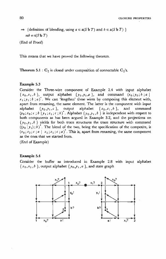
80 CLOSURE PROPERTIES

=* { definition of blending, using a E a(S b T) and b E a(S b T) }

sab E t(Sb T)

(End of Proof)

This means that we have proved the following theorem.

Theorem 5.1 : C 2 is closedunder composition of connectable C 2's.

Example 5.3

Consider the Three-wire component of Example 2.4 with input alphabet {x 0 ,x 1 ,b}, output alphabet {y0 ,y 1 ,a}, and command (x 0 ;y0 ;b;al x 1 ;y 1 ; b ; a) • . We can 'lengthen' these wires by composing this element with, apart from renarning, the same element. The latter is the component with input alphabet {y 0 ,y 1 ,c }, output alphabet {z0 ,z 1 ,b }, and command CYo; zo; c ; b IY 1 ; z 1 ; c ; b )•. Alphabet {y 0 ,y 1 , b } is independent with respect to both components as has been argued in Example 3.2, and the projections on {y 0 ,y 1 , b } yields for both trace structures the trace structure with command ((y 0 I y 1); b )". The blend of the two, being the specification of the composite, is (x 0 ; z 0 ; c ; a I x 1 ; z 1 ; c ; a)·. This is, apart from renarning, the same component as the ones that we started from.

(End of Example)

Example 5.4

Consider the buffer as introduced in Example 2.8 with input alphabet {x 0 , x 1 , b } , output alphabet {y0 ,y 1 , a } , and state graph

Yi 1

•

• xo? • x,? 21~ •

J I/! I,,, . l . j ,,, j . j

. '"'· • CJl, •

J "'l !"j j ./. • • • • 1 xo? a! a! x,? 2

5.6. THE CLOSURE OF C4 81

Alpbahets {x0 ,x 1 ,a} and {y 0 ,y 1 ,b} are independent. This buffer can be composed with another buffer that is obtained from this one by replacing every symbol by its alphabetical successor. The projections of both buffers onto the set of common symbols, i.e. {Jo ,y 1 , b } are the trace structure with command ( (y 0 I y 1) ; b ) • . The other requirements for connectability are satisfied as well and, hence, we may compose these two buffers. A command for the specification of the composite, which is, of course, a two-place buffer, is hard to derive from these two specifications. In fact, any command for the composite is monstrous. Although it is clearly necessary to be able to reason about such a simple com­ponent in an adequate way, we consider it outside the scope of this monograph. Apparently, this is not the appropriate level of abstraction for deriving the specification of a composite. This is, as pointed out in the next chapter, one of the topics of future research.

(End of Exarnple)

5.6. The dosure of C 4

Left to prove for the blend oftwo C 4's are R 4" and R5"'.

Lemma 5.22 : For connectable C 4's S and T, for traces s and t, and for sym­bols a E a(S b T), b E a(S b T), and c E a(S b T) such that b is of another type than a and c

sabtc E t(S b T) 1\ sbat E t(S b T) ~ sbatc E t(S b T)

Proof : We distinguish two cases : (i) c E i(S b T) and (ii) c E o(S b T)

(i) c E i(S b T). Now w~ derive

sabtc E t(S b T) 1\ sbat E t(S b T)

= { definition of blending, using a E a(S b T) and b E a(Sb T) }

(3s 0 ' s I ' t 0 : : sabte E t( s b T) 1\ s obs I at 0 E t( s w T) 1\ s 0 r (as +a T) = s

1\ s 1 f(aS +aT)= ( 1\ t 0 f(aS +aT) = t) ·

~ { Lemma 5.0, since the type of a, being the type of c, is input. Moreover, t(S b T) is prefix-closed and renarning }

(3s0 , t0 :: sabtc E t(S b T) 1\ sabt E t(S b T) 1\ s0bat0 E t(S w T) 1\

sof(aS+aT) = s 1\ t 0 f(aS+aT) = t)

~ { Lemma 5.17, since a is input and b is of another type than a }

(3s0 , t0 :: sabtc E t(S b T) 1\ soabt0 E t(S w T) 1\ s0bat0 E t(S w T) 1\

82 CLOSURE PROPERTIES

sof(aS+aT) = s 1\ l0 f(aS+aT) = l) { calculus and distri bution of projection over concatenation, using

a e a(S b T), b e a(S b T), and c e a(S b T) }

(3so, l0 :: soabl0c f (aS + aT) e t(S b T) 1\ soablo e t(S w T) 1\

s obal 0 e t( S w T) 1\ s 0 f (a S + a T) = s 1\ l o f (a S +a T) = l ) ~ { Lemma 3.5, using c e i(S b T) and the definition of blending }

(3s0 , 10 :: s0abl0c E t(S w T) 1\ s0bal0 e t(S w T) 1\

s0 f(aS+aT) = s 1\ l0 f(aS+aT) = l)

~ {Lemma 5.10}

(3s o , l o : : s obal oe e t( S w T) 1\ s o f (aS +a T) = s 1\ l o f (a S +a T) = l ) ~ { definition of blending, using a e a(S b T), b e a(S b T), and c e a(S b T) }

sbalc E t(S b T)

(ii) c e o(S b T). In this case we derive

sablc E t(S b T) 1\ sbal E t(S b T)

= { definition of blending }

(3so ,si ,lo:: soasibloc E t(S w T) 1\ sbal E t(S b T) 1\ So f(aS +aT) = s

1\ s 1 f(aS+a T) = t: 1\ l0 f(aS+a T) = l) ~ { Lemma 5.1, since the type of a, being the type of c, is output. Moreover,

t(S w T) is prefix-closed and renaming }

(3s0 , lo:: s0abl0c e t(S w T) 1\ soablo E t(S w T) 1\ sbal E t(S b T)

1\ s0 f(aS +aT) = s 1\ lor(aS +aT) = l) ~ {Lemma 5.17, since a is output and b ofanother type than a }

(3so, l0 : : soabl0c e t(S w T) 1\ s0bal0 e t(S w T) 1\

sor(aS +aT) = s 1\ l0 f(aS +aT) = l)

~ {Lemma 5.10}

(3s 0 , l 0 : : s obal 0c e t( S w T) 1\ s o f (a S +a T) = s 1\ l o f (a S +a T) = l ) ~ { definition of blending, using a e a(S b T), b e a(S b T), and c e a(S b T) }

sbatc e t(S b T)

(End of Proof)

5.6. THE CLOSURE OF C4 83

Lemma 5.23 : For connectable C 4's S and T, for trace s, and for symbols a E a(S b T) and b E a(S b T) of different types

sa E t(S b T) 1\ sb E t(S b T) ~ sab E t(S b T)

Proof: We assurne a E i(S b T) and, hence, have to prove

sa E t( S b T) 1\ sb E t( S b T) ~ sab E t( S b T) 1\ sba E t( S b T)

sa E t(S b T) 1\ sb E t(S b T)

= { Lenuna 5.18, using that t(S w T) is prefix-closed }

(3s 0 : : soa E t( s w T) 1\ s ob E t( s w T) 1\ s 0 r (as ...;-a T) = s)

~ { Lenuna 5.14 }

(3s 0 ::soabEt(SwT) 1\ s0baEt(SwT) 1\ s0 r(aS7aT) = s)

~ { definition of blending, using a E a(S b T) and b E a(S b T) }

sab E t(S b T) 1\ sba E t(S b T)

(End of Prooi)

This completes the proof of

Theorem 5.2 : C 4 is closedunder composition of connectable C 4's.

Example 5.5

Consider the C 3 of Example 2.12 with input alphabet { a, d, e } , output alpha­bet { b , c ,j } , and conunand (( (f ; a ) , ( b ; d) )" ;J ; a ; ( c ; e ; b ; d )" ; b ; d )" . As argued in Example 3.6, alphabet { c, e } is independent. Projection on { c, e } yields the trace structure with conunand ( c ; e) • . The trace structure with com­mand ( c ; e )", input alphabet {c } , and output alphabet { e } is a C 1• These two components are connectable. Composition of the two yields the projection of the first trace structure onto { a, b, d ,j } , which is, according to Example 3.6, not a c3. (End of Example)

6

Suggestions for further study

The theory developed in this monograph provides a basefora theory on delay­insensitive circuits. In this chapter we point out a numher of generalizations that might he considered.

In Chapter 3 we noticed already that the requirements for conneetability of trace structures S and T are rather restrictive. The first relaxation considered relates to the requirement that their projeetions on the set of common symbols he the same. This is, provided that the set of common symbols is independent with respect to both trace structures, a sufficient condition to guarantee absence of computation interference. There is nothing wrong, however, with a situation in which the one component is able to receive an input that the other component is never able to produce as output . . An example of this kind is a variable, as we have introduced in Example 2. 7, that is composed with another component that always retrieves a stored value twice before storing a next value in the variable. lt might he sufficient to require

('V a : a E oS n i T : sa E t S f (aS n a T) => sa E t T f (aS n a T)) 1\

('V a : a E o T n iS : sa E t T r (aS n a T) => sa E t S r (aS n a T))

for all traces sEtS f (aS n aT) n t T r (aS n aT). When taking delays into account it is not obvious that this requirement is sufficient to guarantee absence of computation interference. This should he proved again by means of composa­bility of traces as we did in Chapter 4 for the more restrictive composition opera­tor. Expressing requirements in tenns of individual traces is undesirable, how­ever. We would like to express this or a more suitable requirement in tenns of trace structures. How this should he done remains to he seen.

Conneering trace structures by means of independent alphahets seems too res­trictive a requirement as well. Conneering two wires with one another in the usual way, or Conneering a C-element with a Fork to obtain a C-element with

84

85

two outputs is still impossible. We would like to he able to compose trace struc­tures with a set of common symbols that is not independent with respect to each of them. How to incorporate this kind of composition is not clear yet. The fol­lowing might he a possible strategy.

Consider two components that are specified by trace structures S and T respectively. Let C he the set of common symbols and let C he independent with respect to neither S nor T. Fortrace structure S this means that there is a trace tEtS and a symbol a E c niS such that (t fC)a EtS re and ta f1_ tS (or something similar with C replaced by aS\ C). In other words, there are still communications to he performed by means of the symbols of the complement with respect to aS before input a can he received by the component. The two environments that the environment of S is partitioned into by C and aS \ C cannot communicate with the component independent of one another. They need additional information on each other's progress. Therefor we could intro­duce an alphabet D of fresh symbols via which the two environments can directly communicate. In order to reflect these communications traces of S should he interspersed with symbols of D in a suitable way. The component-environment pair now becomes a triple : ·

Having clone something similar with trace structure T, using the same set of symbols D, we can hl end the new S and T, provided that S f ( C U D) and Tf(C U D) meet certain conditions, e.g. S f(C U D) = Tf(C U D).

The problem of course is the interspersion of traces of S with symbols of D. One of the questions is what requirements to impose upon the resulting trace structure. A necessary, and possibly sufficient, condition seems to he that the projectionsof the new trace structure onto C U D and (aS\ C) U D he delay­insensitive. A second question is how to find D and how to construct the desired trace structure. A trivial way is to conceive one of the environments, E 0 say, as a pass-through for all incoming signals. This means that there is a one-to-one correspondence between input symbols of C and output symbols of D and between output symbols of C and input symbols of D. (Input and output is

86 SUGGESTIONS FOR FURTHER STUDY

here with respect to E0.) Moreover, in the specification of the communications via C and D every input is foliowed by its corresponding output and so repeat­edly. The specification of the communications via D and aS \ C is in this case the same as the one via C and aS \ C with every symbol of C replaced by its corresponding symbol in D .

Once we have properly relaxed the requirements for connectability and have proved the absence of transmission and computation interference we have to answer the question whether and how to incorporate multiple transitions on a wire in our forrnalism. As we have pointed out in the introduction, we can allow multiple transitions on a wire in the presence of a data valid wire that signals the validity of a voltage level on the first wire. This kind of protocol is aften used for data transmission. A high level on a wire represents a logica! one and a low level on that wire a logica! zero. Having n data wires we can convey 2n different values.

Not using a data valid wire we eneode data by a so-called m out of n cad­ing. Ha ving n wires a transition on exactly m of them, 0 ~ m ~ n, represents a value. In this way we can convey (~)different values. For fixed n the maximum value of (~) is asymptotically 2n I yn. Notice that we have used a 1 out of 2 coding for the data transmission in the examples.

The advantage of data transmission with a data valid wire is the smaller number of wires needed and the availability of circuits that can handle data encoded in this way, e.g. adders and multipliers. The number of wires used to convey data, however, is typically 8, which makes, tagether with the data valid wire, a total of 9 wires required. An m out of n coding requires 11 wires for 8 bits of inforrnation,which does not seem to be too large a difference. An interest­ing question is how to build arithmatical circuits that can handle data encoded in this way. It might just be that this encoding seems more difficult only because we are used to the other one.

A question, which is aften posed, is whether there exists a (finite) base for delay-insensitive circuits, i.e. a (finite) set of delay-insensitive circuits by means of which we can obtain all delay-insensitive circuits by composition. Once we have relaxed the requirements for composition of components this is a valid question. It might be that there exists a base consisring of just a few elements, which would make a gate array approach for the irnplementation of a component as chip very attractive. Ciosure properties of classes rnay be helpful in finding such a set. Using, for instance, the composition operator as defined in Chapter 3 we cannot obtain a C 4 from C 2's. This means that an arbiterlike device necessarily belongs to a base. It is very likely that the dosure properties derived in Chapter 5 hold for less restrictive composition operators as well.

Trace theory as it is used here provides the first step towards a high level specification language that we would like a silicon compiler, our ultirnate goal, to be able to accept. Specifying circuits at the current level of abstraction is a nuisance. Anotlier topic of research, therefore, is how to translate specifications

87

written at a higher level of abstraction, like for instanee the specifications in [ 12], into specifications that satisfy the rules for delay-insensitivity and still have, in some sense, the same meaning. One can think, for example, of adding symbols to guarantee proper communications.

7 Concluding remarks

In dus monograph we have discussed specifications of circuits when making no assumptions on wire delays. This has led to a definition and a classification of delay-insensitive circuits. Moreover, we have proposed a composition operator that we have shown to warrant internal communications that are free of transmission and computation interference. Three of the four classes turn out to be closed under this composition operator. A few final remarks on the results obtained seem to be apposite.

C 1, C 2, and C 3 arose from an intuitive understanding of delay-insensitive cir­cuits and of decisions that are to be made in the component and in the environ­ment. Since C 3 tumed out not to be closedunder the composition operator pro­posed, the need for a larger, still physically interpretable, class developed. c4 is a class that satisfies these requirements, which makes C 3, in fact, obsolete.

Petri nets [7] are frequently used for the specification of delay-insensitive cir­cuits. They suffer, however, from a canonical form problem, i.e. distinct Petri nets may specify the same circuit. This makes it hard to capture properties of delay-insensitive circuits in terrns of Petri nets. Trace structures do not suffer from this canonical form problem and are, therefore, more suited to define and classify delay-insensitive components. Petri nets can, like our program texts or state graphs, very well be used for the representation of trace structures. The question whether there is a representation that should be preferred to the others is not easily answered. Probably it depends on the circumstances under which they are · to be used and on the question by whom they are to be used.

We have confined our attention to components that satisfy the rules for delay-insensitivity and we have defined for that class of components a composi­tion operator. The advantage of this approach is that it is not necessary to take wire delays into account when composing components : the blend has been shown in Chapter 4, with some effort but we only have to do it once, to be a proper composition operator for this kind of components. This is opposed to the

88

89

approach taken in [ 12] where a larger class of components is considered. When composing this kind of components, however, one cannot simply use the blend but one needs a much more complicated composition operator, called agglutina­tion. The result of such an agglutination is not easily computed. Confining the class of components to he considered seems to he a better approach for dealing with wire delays.

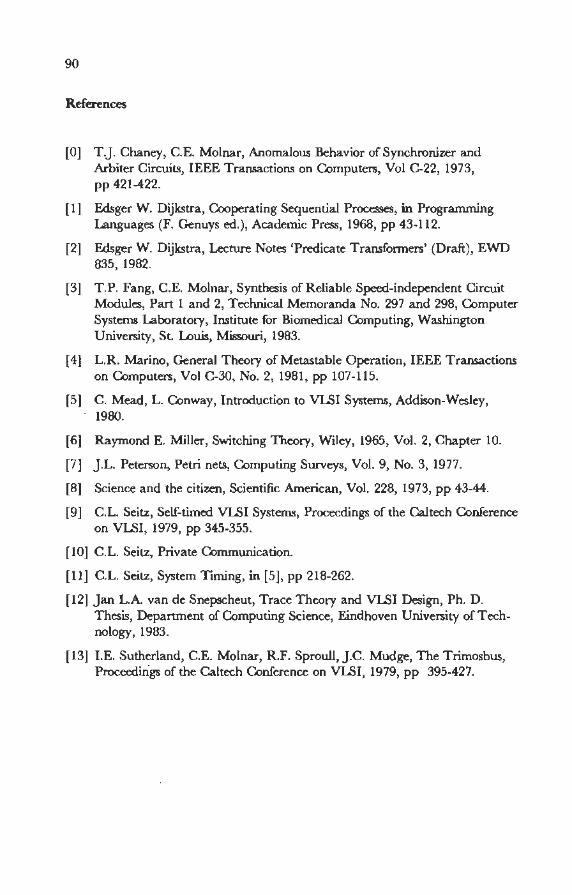
90

References

[0] T.J. Chaney, C.E. Molnar, Anomalous Behavior of Synchronizer and Arbiter Circuits, IEEE Transactions on Computers, Vol C-22, 1973, pp 421-422.

[ 1] Edsger W. Dijkstra, Cooperating Sequentia! Processes, in Programming Languages (F. Genuys ed.), Academie Press, 1968, pp 43-112.

[2] Edsger W. Dijkstra, Lecture Notes 'Predicate Transformers' (Draft), EWD 835, 1982.

[3] T.P. Fang, C.E. Molnar, Synthesis of Reliable Speed-independent Circuit Modules, Part 1 and 2, Technica! Memoranda No. 297 and 298, Computer Systems Laboratory, Institute for Biomedical Computing, Washington University, St. Louis, Missouri, 1983.

[ 4] L.R. Marino, General Theory of Metastable Operation, IEEE Transactions on Computers, Vol C-30, No. 2, 1981, pp 107-115.

[5] C. Mead, L. Conway, Introduetion to VLSI Systems, Addison-Wesley, 1980.

[6] Raymond E. Miller, Switching Theory, Wiley, 1965, Vol. 2, Chapter 10.

[7] J.L. Peterson, Petri nets, Computing Surveys, Vol. 9, No. 3, 1977.

[8] Science and the citizen, Scientific American, Vol. 228, 1973, pp 43-44.

[9] C.L. Seitz, Self-timed VLSI Systems, Proceedings of the Caltech Conference on VLSI, 1979, pp 345-355.

[ 10] C.L. Seitz, Private Communication.

[11] C.L. Seitz, System Timing, in [5], pp 218-262.

[12] Jan L.A. van de Snepscheut, Trace Theory and VLSI Design, Ph.D. Thesis, Department ofComputing Science, Eindhoven University ofTech­nology, 1983.

[13] I.E. Sutherland, C.E. Molnar, R.F. Sproull, J.C. Mudge, The Trimosbus, Proceedings of the Caltech Conference on VLSI, 1979, pp 395-427.

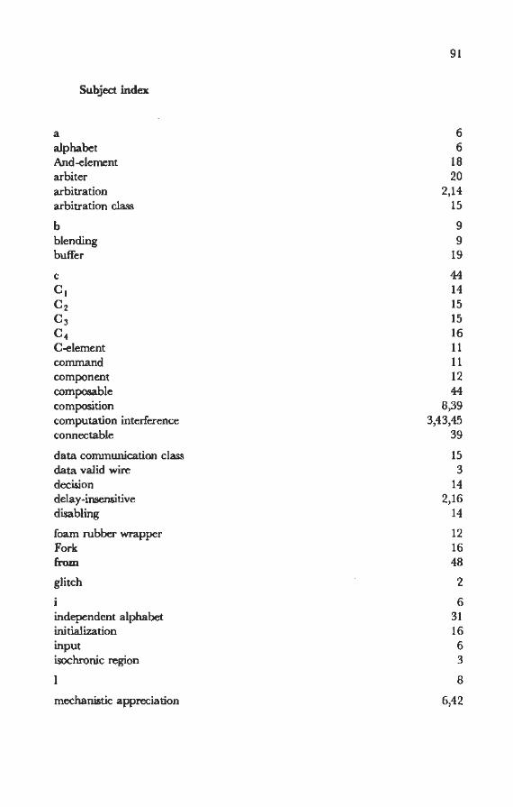
91

Subject index

a 6 alp ha bet 6 And-element 18 arbiter 20 arbitration 2,14 arbitration class 15

b 9 blending 9 buffer 19

c 44 cl 14 C2 15 c3 15 c4 16 C-element 11 conunand 11 component 12 composable 44 composition 8,39 computation interterenee 3,43,45 connectable 39

data communication class 15 data valid wire 3 decision 14 delay-insensitive 2,16 disabling 14

foam rubber wrapper 12 Fork 16 from 48

glitch 2

i 6 independent alphabet 31 initialization 16 input 6 isochronie region 3

8

mechanistic appreciation 6,42

92

Merge 16 mm 48 m out of n coding 86

0 6 output 6

parity counter 17 Petri net 88 pref 8 prefix 8 prefix-dosure 8 projection 7

QRL 78

Ro 13 R, 13 R2 13 R 3 13 R• 14,16 Rs 14

8emaphore 79 state graph 16 symbol 6 synchronization class 14

t 6 TR 11 trace 6 trace structure 6 transmission interference 3,43,45

variabie 18

w 8 weaving 8 Wire 7

93

Samenvatting

In dit proefschrift wordt een definitie en een classificatie van en een compositie­methode voor vertragingsongevoelige circuits besproken. Dit zijn circuits waar­voor geen aannamen gemaakt worden omtrent vertragingen in verbindings­draden of omtrent de snelheid waarmee zo een circuit reageert op input sig­nalen. De reden voor de bestudering van dergèlijke circuits is tweeerlei. Enerzijds bestaan er circuits die niet altijd binnen een bepaalde tijd een berekening heb­ben uitgevoerd. Dit betekent dat er in de specificatie van een circuit dat met zo een circuit wordt verbonden niet van uitgegaan mag worden dat input signalen binnen een zekere tijd na de output signalen zullen kunnen worden ontvangen. Anderzijds blijkt dat door het verkleinen van geintegreerde schakelingen de ver­tragingstijden van elektrische signalen in verbindingsdraden toenemen ver­geleken met de schakeltijden van transistoren, zodat vertragingen in draden niet langer verwaarloosd mogen worden.

Een viertal klassen van vertragingsongevoelige circuits wordt op axiomatische wijze gedefinieerd. Drie van deze klassen blijken gesloten te zijn onder de voor­gestelde compositieoperator, terwijl de vierde dit niet is. Voor de specificatie en compositie van circuits en voor de geslotenheidsstellingen wordt gebruik gemaakt van trace theory. Dit is een theorie van symboolrijen en verzamelingen symbool­rijen.

Bij het samensteHen van circuits dient aan twee voorwaarden te zijn voldaan. Ten eerste moet gegarandeerd zijn dat elektrische signalen op een verbindings­draad niet met elkaar kunnen interfereren. Door geen aannamen te maken over vertragingen betekent dit dat hooguit één signaal per draad is toegestaan. Daar­naast mag een elektrisch signaal pas bij een circuit arriveren als dat circuit, vol­gens zijn specificatie, in staat is tot de ontvangst van dat signaal. Van de in dit proefschrift voorgestelde compositieoperator wordt aangetoond dat bij compositie van vertragingsongevoelige circuits aan deze beide voorwaarden is voldaan.

94

Curriculum vitae

De schrijver van dit proefschrift is op 11 juni 1953 geboren te Den Helder. Na het eindexamen Gymnasium-P in 1971 te hebben afgelegd aan het Drachtster Lyceum te Drachten is een aanvang gemaakt met de studie wiskunde aan de Technische Hogeschool Eindhoven. In februari 1980 wordt het diploma wiskun­dig ingenieur behaald, na afstudeerwerk onder leiding van prof.dr. N.G. de Bruijn. Tot april 1982 wordt daarna gewerkt als medewerker van de Sector Informatica aan het Dr. Neher Laboratorium van de PTf in Leidschendam. Sinds 15 april 1982 wordt als wetenschappelijk medewerker aan de Onderafdel­ing der Wiskunde en Informatica van de Technische Hogeschool Eindhoven gewerkt in de vakgroep Informatica onder leiding van prof.dr. M. Rem. Van september tot en met november 1983 is bovendien als research fellow onderzoek verricht op het gebied van vertragingsongevoelige systemen onder leiding van prof.dr. C.E. Molnar aan de Washington University te St. Louis, Missouri.

STELLINGEN

behorende bij het proefschrift

Classification and composition of delay-insensitive circuits

van

Jan Tijmen Udding

Eindhoven, 25 september 1984

0. Voor iedere natuurlijke q en m waarvoor geldt m =I= 1, q ~ 2m + 1, q (1 of 3mod6) en m = ( 1 of 3mod6) bestaan er twee Steiner triple systems van orde q (op dezelfde verzameling punten) die precies een Steiner triple sys­tem van orde m gemeen hebben.

lit : J.l. Hall and J.T. Udding, On the Intersection of Pairs of Steiner Tri­ple Systems, Proc. Kon. Akad. v. Wet., ASO, 1977, pp 87-100.

1. Voor gegeven alfabet A en prefix-closed trace set U heeft de vergelijking T Ç A • : T = Ub s. T precies één oplossing die t: bevat indien voor iedere u E u geldt 1 (u r s.A ) ~ I (u rA ). lit : J.T. Udding, On recursively defined sets of traces, Intern Memoran­

dwn, JTUOa, 1983.

2. De klassen van vertragingsongevoelige trace structures die voldoen aan de regels R 0 tot en met R 4" en aan ofWel R 5' dan wel R 5" zijn gesloten onder compositie van connectable trace structures.

lit : Dit proefschrift.

3. Het is opvallend en valt te betreuren dat in zo weinig boeken over tralie­theorie aandacht wordt besteed aan eigenschappen van morfismen.

4. Het blijven uitbreiden van het relationele model draagt geenszins bij tot een goede fundering van de theorie over informatiesystemen.

5. Imperatieve programmeertalen zijn een erfenis uit de tijd dat het doel van een taal nog was het programmeren van een machine. Nu machines er zijn om onze programma's uit te voeren, dient aanmerkelijk meer aandacht te worden besteed aan het gebruik van non-imperatieve programmeertalen dan momenteel het geval is.

6. Bij het beschrijven van fysische objecten door middel van een wiskundig model dienen objecten die in het model van elkaar verschillen te correspon­deren met objecten die om fysische redenen van elkaar verschillen. Petri netten dienen derhalve niet gebruikt te worden voor de specificatie van ver­tragingsongevoelige systemen.

7. Slechte ervaringen met inadequate formalismen hebben geleid tot een schromelijke onderschatting van de mogelijke rol van formalismen.

8. Het idee dat bewijsvoering gereduceerd kan worden tot formulemanipulatie getuigt van een schromelijke overschatting van de mogelijke rol van for­malismen.

9. Onderzoek heeft bij uitstek een individueel karakter. De te ver door­gevoerde demokratisering van het universitair bestel in Nederland is dan ook funest voor het verrichten van goed en origineel onderzoek.

10. Gelukkig is, zoals de naam al zegt, temporele logica maar tijdelijk.

11. Binnenkort zal de zogenaamde 'school met de computer' zijn intrede doen in de strijd om de gunst van de leerplichtige. De suggestie als zou een der­gelijke school een streepje voor hebben op andere scholen is onjuist en dient als misleiding te worden aangemerkt.