Classification of Mass spectrometry data using

principal components analysis, Bayesian

MCMC modelling and a deterministic peak

finding algorithm.

William Browne (University of Nottingham)

Joint work with Kelly Handley and Ian Dryden

1

Outline

1. Background

2. Data sets and Questions

3. Principal Components

4. MCMC method

5. Peak finding algorithm

6. Cross validation

7. Further Work

2

Mass spectrometry

• Invented by J.J. Thomson in early 20th century.

• Description:

A substance is bombarded with an electron beam having sufficient

energy to fragment the molecule. The positive fragments which are

produced are accelerated in a vacuum through a magnetic field and

are sorted on the basis of mass-to-charge ratio. Since the bulk of

the ions produced in the mass spectrometer carry a unit positive

charge, the value m/z is equivalent to the molecular weight of the

fragment.

3

MALDI and SELDI TOF data

• Two types of mass spectrometry used in proteomics to identify

proteins that are associated with disease states such as cancer.

• MALDI - matrix-assisted laser desorption/ionization

• SELDI - surface-enhanced laser desorption/ionization

• TOF - time of flight

MALDI was developed in 1987 whilst SELDI is an improved

method that was invented in the early 1990s. Both produce mass

spectographs.

4

Example Mass spectrograph

Below is a mass spectrograph for a melanoma patient. Note that

M/Z values below 2000 are removed due to noise.

5000 10000 15000 20000 25000 30000

010

2030

4050

60

mzvalues

data

[1, ]

5

Close up of start of mass spectrograph

Below is a close up of the first 2000 (out of 13951) stored M/Z

values in the mass spectrogram showing how it is a series of

humps/peaks.

2000 2500 3000 3500 4000

02

46

810

12

mzvalues[1:2000]

data

[1, 1

:200

0]

6

Dataset 1: The Breast Cancer Dataset

• consists of 144 SELDI mass spectrographs from 2 independent

experiments.

• each spectrum is either a control or has been treated with the

chemotherapeutic agent Taxol.

• there are 3 drug groups MCF7/ADR, MCF7 and T47D.

• MCF7/ADR is chemoresistant, MCF7 and T47D are

chemosensitive.

• each experiment lasted for 4 days with observations every 24

hours.

• 3 observations (A,B,C) were taken after each 24 hour time period.

7

Dataset 1: The Breast Cancer Dataset

8

Dataset 2: The Melanoma Dataset

• Consists of 205 MALDI mass spectrographs of serum samples.

• The serum samples are taken from melanoma patients.

• Each patient is classified as either an early or late stage

Melanoma.

• There are 101 early stage (AJCC Stage 1) and 104 late stage

(AJCC Stage IV) patients.

9

Dataset 2: The Melanoma Dataset

10

Questions

We are interested in looking for differences between mass

spectrographs for the various groups in our datasets. Our

objectives are primarily dimension reduction and classification

(rather than inference).

We will firstly look at a technique that reduces the spectrographs

of length 13,950 M/Z values to a manageable number of derived

variables that explain most of the variability in the data.

We will then consider other techniques that reduce the

dimensionality to a group of easily interpretable variables. In

particular we are looking for potential biomarkers - individual

peptides that might help in classification

11

Specific Questions

For the breast cancer dataset we are interested in looking for:

• Where are there differences between the control and treated

spectra within the same drug groups?

• Where are there differences between the 3 control spectra?

For the melanoma dataset we only have 2 groups and so interest

lies simply in looking for differences between the early and late

stage spectrographs.

We will start by considering principal components analysis.

12

Principal Components

• Principal components analysis (PCA) tries to describe the

important variability in the data in a reduced number of

dimensions.

• Consider n observation vectors x1,x2, ...,xn each of length p.

The sample mean is

x̄ =1

n

n∑

i=1

xi

• The sample covariance matrix is the n× n matrix

S =1

n

n∑

i=1

(xi − x̄)(xi − x̄)T

13

• The eigenvectors γj of the matrix S are the principal components

(PCs) with corresponding decreasing eigenvalues λj

(j = 1, ..,min(p, n− 1)). The PC score sij for the ith observation

on the jth principal component is

sij = γTj (xi − x̄)

• We will be calculating principal components of a subset of each

dataset and using these to classify the remainder of the dataset

using Fisher’s linear discriminant rule.

14

Problems with a PCA approach

• On the plus side we will see that PCA does well in the

cross-validation exercises we perform later and it does reduce the

dimension of the data used.

• However, classification using PCA uses all of the data to form the

PCs and these PCs are not necessarily easy to interpret.

• What we would like is to be able to identify points in the data

where our groups differ.

Question: Are there ways of classifying using fewer pieces of

information?

15

t tests and False Discovery Rates

• One possibility is simply to compare groups at each of the 13,950

M/Z values via 2 sample t-tests.

• We considered a multivariate version of this approach (Dryden et

al. 2005) using dataset 1 and the 4 day structure to create

4-vectors and using Hotellings T 2 statistic.

• We considered both FDR (Benjamini and Hochberg, 1995) and a

variance offsetting approach to account for the multiple

comparisons problem and found some interesting differences on the

spectrographs between pairs of groups.

• We would however prefer an approach that accounts for more of

the structure in the dataset.

16

A model based approach

• Ideally we would like to fit some functional form to each of our

scans (spectrograms), where the function contains interpretable

parameters.

• The science suggests that a scan will consist of a series of peaks

at differing M/Z values.

• One way to model this is with a mixture of (scaled) normal

curves to represent the peaks. Each normal curve will have a

position (mean), variance and scale factor (height) and the sum of

these normal curves will be used to approximate the observed scan.

17

Too many parameters ?

• We have many scans and so to compare across scans we will need

to have some shared parameters and the non-shared parameters

will then be used for classification.

• Peak means - these will be shared by all scans.

• Peak variances - the scans suggest these increase with increased

M/Z value so we decided to make the peak sds ∝ the peak mean

values.

• Peak heights - these will be allowed to vary across scans and will

hence be used for classification.

18

A model/likelihood

• The model used for each datapoint yij on the spectrum is

yij ∼ N(θij , τ−1) where

θij =K∑

k=1

hkj(ξµ2k)

− 12 exp

(

−1

2(ξµ2

k)−1(mz(i)− µk)

2

)

Here i indexes the M/Z values on each scan, k indexes the peak

number and j indexes the scan number.

We have hkj - the height of the kth peak on the jth scan.

µk - the position of the kth peak and ξ a scale factor that links the

variance of the peak with µ2k. The function mz(i) returns the ith

M/Z value.

19

A Bayesian model

We wish to use MCMC to estimate parameters in this model. We

will assume K the number of peaks is fixed. Then we will need

priors for τ, ξ, hkj and µk.

These will be as follows:

p(τ) ∼ Gamma(0.001, 0.001)

p(ξ) ∼ Uniform(0, 0.01)

p(hkj) ∼ Uniform(0, 100)

p(µ1, . . . , µK) ∝ e−β(∑

i,j |µi−µj |<R)

i.e. a Strauss prior for the means that encourages them to keep

apart and avoids label switching.

20

MCMC algorithm

The MCMC algorithm will update the four groups of parameters,

τ, ξ, hkj and µk in turn. τ has a Gamma conditional posterior

distribution and can be updated using Gibbs sampling but for all

other parameters we use random walk Metropolis sampling.

We use the adapting procedure of Browne and Draper (2000) to

tune the proposal distributions prior to the MCMC burnin. This

method alters the proposal variances by comparing acceptance in

batches of 100 iterations and aims for an acceptance rate of 50%.

We will aim to find the MAP estimate from the MCMC chains that

we produce. The algorithm is still tremendously slow as the y

matrix is of size 13,950 by 144/205(N) for the two datasets and if

we consider K peaks then we have K ∗ (N + 1) + 2 parameters to

estimate.

21

Speeding up the algorithm

1. To speed up the code we store the values of θij , which occur

prominently in the joint posterior at the start. We then modify

them via addition and subtraction rather than recalculating them

from scratch wherever possible during the algorithm.

2. Secondly we consider a ‘truncated’ Normal likelihood where we

ignore the effects of a peak on θij values that are > 4 peak sds from

the peak mean.

22

Application to datasets

We applied the MCMC sampler to small sections of both the breast

cancer and the melanoma datasets. Each section ranged over

roughly the same m/z values. For breast cancer from 6800 Da to

8400 Da and melanoma from 6000 Da to 8400 Da. For each section

we choose K = 8 peaks. The adapting period took 2,100 iterations

for each dataset and we than ran for 1000 burnin iterations and

5000 stored iterations from which we selected the MAP estimates.

23

Tabular summary

Breast cancer

param. µ1 µ2 µ3 µ4 µ5 µ6 µ7 µ8

MAP 6917 7027 7207 7437 7692 7907 8110 8348

with ξ = 0.000048 and τ = 2.1996

Melanoma

param. µ1 µ2 µ3 µ4 µ5 µ6 µ7 µ8

MAP 6056 6461 6650 6762 6864 7793 7963 8165

with ξ = 0.000035 and τ = 6.6729

24

Plots for Breast cancer dataset

7000 7500 8000

−20

−10

010

20

adcon day 1

mzvector

data

MAP

DATA

7000 7500 8000

−20

−10

010

20

adcon day 2

mzvector

data

MAP

DATA

7000 7500 8000

−20

−10

010

20

adcon day 3

mzvector

data

MAP

DATA

7000 7500 8000

−20

−10

010

20

adcon day 4

mzvector

data

MAP

DATA

25

Plots for Melanoma dataset

6000 6500 7000 7500 8000

−50

050

stage 1

m/z value

data

6000 6500 7000 7500 8000

−50

050

stage 4

m/z value

data

26

Problems with MCMC approach

1. The approach is simply not computationally feasible for a

cross-validation exercise.

2. We are currently relying on a fixed K for the number of peaks,

although we could use reversible jump MCMC to cure this.

3. Although the Strauss prior avoids label switching, peaks can be

missed by the MCMC algorithm as it converges to a local

maximum.

4. To this end ‘good’ starting values are essential!

27

Motivation for a simpler approach

The speed of the MCMC method as it stands prohibits its serious

use however if we had a ‘good’ starting position then running

MCMC or something similar for a limited time may be feasible.

We therefore look for an approach to give us such a starting

position. Given the MCMC approach involves a series of peaks at

various locations on the scan with heights varying across scans and

with sd proportional to the mean, we look for a deterministic

approach.

28

Deterministic Peak finding

The MCMC approach considers K peaks for N scans, each peak

defined by three parameters, a position, µk, a variance (ξµ2k) and a

height hkj . We will simplify matters by assuming ξ is a known

constant that we can easily measure by looking at the scans. We

then have a 2 step procedure where we iteratively find the best

position to fit a peak (conditional on existing peaks) and then

calculate the required heights of this peak for each scan so that the

fitted function fits exactly at the peak location.

29

Deterministic Peak finding algorithm

Let yij be the ith location in the jth scan, fk(x) = N(µk, ξµ2k) be a

Gaussian kernel for the kth peak and hkj be the height term for the

kth peak on the jth scan. Then for peak k we form

eij = yij −k−1∑

p=1

hpjfp(mz(i))

where mz(i) returns the M/Z value for the ith location. Here eij is

in effect the residual at location i on scan j when k − 1 peaks have

been fitted. For the first peak we have eij = yij and we now want

to choose a location to place the first peak.

30

Deterministic Peak finding algorithm

For the kth peak we do the following:

Step 1: Find i such that∑

j eij is maximised. The kth peak will

then have mean location mz(i). Note that as we are only

considering positive peaks we prefer to sum the eij rather than

their squares.

Step 2: We now have k peak locations and we wish to calculate the

associated hkj . Here our aim is to fit exactly at the peak locations

for each scan. We will discuss this step further on the next slide.

Step 3: Recalculate the eij = yij −∑k

p=1 hpjfp(mz(i)).

31

Heights calculation

Let us assume we have K peaks and we wish to match at the peak

mean locations. Then let lk be the location of the kth peak with

corresponding M/Z value µk = mz(lk) and we require for scan j

h1jf1(µ1) + h2jf2(µ1) + . . .+ hKjfK(µ1) = yl1j

h1jf1(µ2) + h2jf2(µ2) + . . .+ hKjfK(µ2) = yl2j

. . .

h1jf1(µK) + h2jf2(µK) + . . .+ hKjfK(µK) = ylKj

This is simply K linear equations in K unknowns and in matrix

form the solution is H = F−1Y.

32

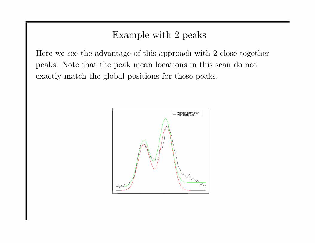
Example with 2 peaks

Here we see the advantage of this approach with 2 close together

peaks. Note that the peak mean locations in this scan do not

exactly match the global positions for these peaks.

6800 6900 7000 7100

05

1015

20

m/z value

data

without correctionwith correction

33

Comments on method

It is worth commenting here that this method was originally

considered only as a way of generating starting values for MCMC.

Although as we will see it is useful in its own right.

As we add the kth peak we have to invert N k × k matrices and so

the method is initially very fast although for a large number of

peaks (k > 100) computation time may be more of an issue.

We tested the method on the same small pieces of each dataset as

MCMC and get the following results:

34

Comparison with MCMC 1

Breast cancer

param. µ1 µ2 µ3 µ4 µ5 µ6 µ7 µ8

Peak 6913 7013 7274 7450 7688 7903 8102 7118

MCMC 6917 7027 7207 7437 7692 7907 8110 8348

Note the broad agreement for 6 of 8 peaks with the peak finding

assessing that 2 peaks around 7200 are more appropriate than an

additional peak at 8348. Note MCMC is constrained by its starting

values and so will not be able to reach the peak finding solution

easily.

35

Plots for Breast cancer dataset

7000 7500 8000

−20

−10

010

20

adcon day 1

m/z values

data

FITTED

DATA

7000 7500 8000

−20

−10

010

20

adcon day 2

m/z values

data

FITTED

DATA

7000 7500 8000

−20

−10

010

20

adcon day 3

m/z values

data

FITTED

DATA

7000 7500 8000

−20

−10

010

20

adcon day 4

m/z values

data

FITTED

DATA

36

Comparison with MCMC 2

Melanoma

param. µ1 µ2 µ3 µ4 µ5 µ6 µ7 µ8

Peak 6543 6451 6646 6744 6856 7777 7937 8154

MCMC 6056 6461 6650 6762 6864 7793 7963 8165

Again we have general agreement between the two approaches with

7 of the peaks in roughly the same position. Looking at the scans

by eye there aren’t really 8 peaks and so the location of the eight

peak is rather arbitrary!

37

Plots for Melanoma dataset

6000 6500 7000 7500 8000

−50

050

stage 1

mz value

6000 6500 7000 7500 8000

−50

050

stage 4

mz value

38

Cross validation experiment

To compare the performance of the 3 approaches discussed we

considered a cross validation experiment. Unfortunately MCMC

was not computationally feasible to be used here.

For each dataset we randomly split the data into two parts, the

training set ( 23 ) and test set ( 13 ).

Note that these splits were performed within each type of scan so

for the breast cancer dataset, the 24 ADC scans were allocated 16

to training and 8 to test etc.

For each dataset 100 such random splits of the dataset were created

and we were interested in average correct classification of the test

data.

39

Assessing the methods - PCA

We firstly take the training set and calculate PCs based on this set.

The resulting principal components are then added in turn and the

classification of the test data based on Fisher’s linear discriminant

rule (applied to the training data) is evaluated after each PC is

added.

This will result in a percentage correct classification for each split,

for each number of PCs and these can be plotted against number of

PCs.

In the graphs that follow we also use the 100 splits to generate a

mean performance and confidence intervals.

40

Assessing the methods - peak finding

Again we firstly take the training set and this time calculate the

first 50 peaks using the peak finding algorithm on the training set.

We then take the test data and evaluate the heights of these 50

peaks for the test data.

It is not clear that the largest peak is the best classifier so we

instead choose the order of introducing the peaks via other rules.

Firstly for both datasets we assess which peaks best predict the

training data using linear discriminant analysis.

Secondly for the melanoma dataset we also consider a simple t test

approach comparing t statistics for the difference between groups in

the training set for each peak.

41

Assessing the methods - peak finding (2)

Having sorted the peaks into an order using one of the above

methods we now add them in one at a time as with the PCs in the

PCA approach.

The classification of the test data is then based on Fisher’s linear

discriminant rule (applied to the training data) which is evaluated

after each peak is added.

This will result in a percentage correct classification for each split

for each number of peaks and these can be plotted against number

of peaks. In the graphs that follow we also use the 100 splits to

generate a mean performance and confidence intervals.

Note the whole procedure is automated in a C program that calls R

several times to perform the bulk of the procedure apart from the

computationally expensive peak finding which is done in C.

42

Results for breast cancer : All 100 runs

0 10 20 30 40 50

020

4060

8010

0

fitted heights − best classification

no of peaks used to classify

perc

enta

ge c

orre

ct c

lass

ifica

tions

Breast Cancer Dataset

0 20 40 60 80

020

4060

8010

0

original PCA − training(2/3)test(1/3)number of datavalues =

13952

no of pc’s used to classify

perc

enta

ge c

orre

ct c

lass

ifica

tions

43

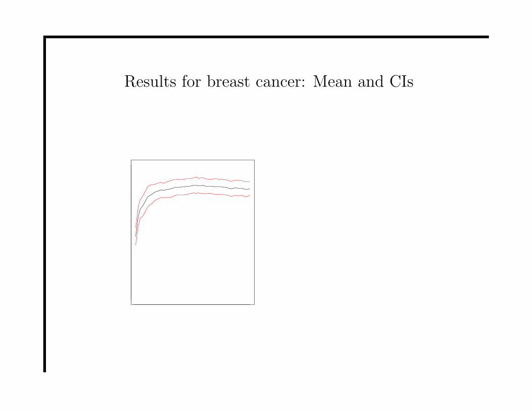
Results for breast cancer: Mean and CIs

0 10 20 30 40 50

020

4060

8010

0

peak fitting − best classification

no of peaks

% c

orre

ct c

lass

ifica

tion

Breast Cancer Dataset

0 20 40 60 80

020

4060

8010

0

pca

no of pc’s

% c

orre

ct c

lass

ifica

tion

44

Comments on Breast cancer results

• PCA got 90.1% correct classification but to reach this level 54

PCs were required.

• Peak finding got 85.1% correct classification using best

classification of training set and this was obtained with only 27

peaks (73% with first 5 peaks).

• A peak at around 8104 was chosen as first peak 56% of the time

and 75% of the time in the first 5 peaks.

• This location differentiates well between ADC, TDT and the

other 4 groups.

45

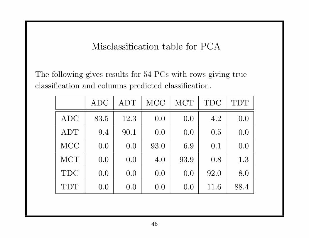
Misclassification table for PCA

The following gives results for 54 PCs with rows giving true

classification and columns predicted classification.

ADC ADT MCC MCT TDC TDT

ADC 83.5 12.3 0.0 0.0 4.2 0.0

ADT 9.4 90.1 0.0 0.0 0.5 0.0

MCC 0.0 0.0 93.0 6.9 0.1 0.0

MCT 0.0 0.0 4.0 93.9 0.8 1.3

TDC 0.0 0.0 0.0 0.0 92.0 8.0

TDT 0.0 0.0 0.0 0.0 11.6 88.4

46

Misclassification table for peak finding

The following gives results for 27 peaks with rows giving true

classification and columns predicted classification.

ADC ADT MCC MCT TDC TDT

ADC 76.8 15.5 0.2 0.0 7.5 0.0

ADT 8.8 87.5 0.0 0.1 3.1 0.5

MCC 0.0 0.9 88.4 10.0 0.1 0.6

MCT 0.0 0.5 10.2 85.8 0.7 2.8

TDC 0.4 0.2 0.0 0.0 89.8 9.6

TDT 0.1 0.0 0.0 0.0 17.3 82.6

47

Chosen peaks

The following table gives the 9 peaks that are chosen most often in

the first 5 peaks in the 100 iterations.

peak M/Z 1st 2nd 3rd 4th 5th Total

1 8104 56 14 2 2 1 75

2 7452 25 34 2 0 1 62

3 5416 0 15 9 10 10 43

4 11133 1 1 14 9 9 34

5 11701 0 0 22 4 5 31

6 4392 16 0 1 5 6 28

7 4345 0 4 4 5 9 22

8 4881 1 9 6 0 1 17

9 10232 0 4 1 6 6 17

48

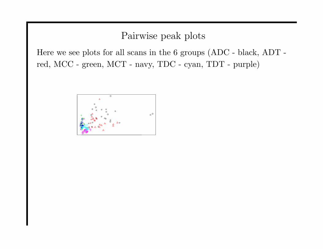
Pairwise peak plots

Here we see plots for all scans in the 6 groups (ADC - black, ADT -

red, MCC - green, MCT - navy, TDC - cyan, TDT - purple)

0 5 10 15

02

46

810

1214

Peak2

Pea

k1

2 4 6 8 10

02

46

810

1214

Peak3

Pea

k1

2 4 6 8

02

46

810

1214

Peak4

Pea

k1

2 4 6 8 10 12

02

46

810

1214

Peak5

Pea

k1

49

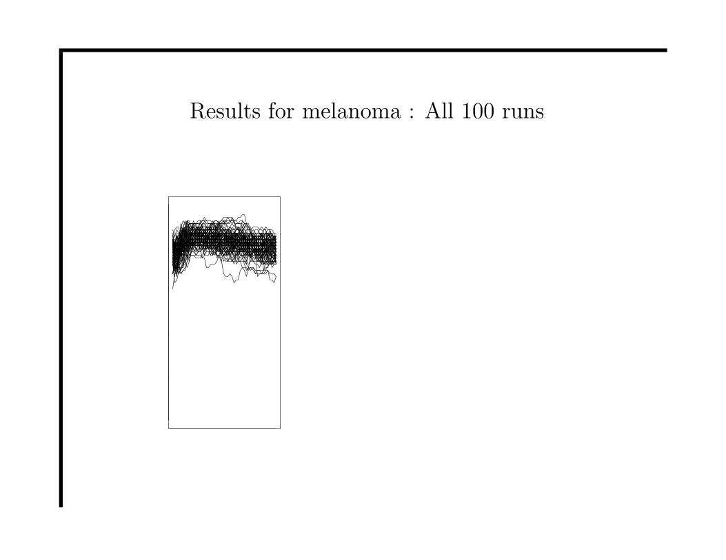
Results for melanoma : All 100 runs

0 10 20 30 40 50

020

4060

8010

0

fitted heights − t−tests

no of peaks used to classify

perc

enta

ge c

orre

ct c

lass

ifica

tions

Melanoma Dataset

0 10 20 30 40 50

020

4060

8010

0

fitted heights − best classification

no of peaks used to classify

perc

enta

ge c

orre

ct c

lass

ifica

tions

0 20 40 60 80 100 120 140

020

4060

8010

0

original PCA − training(2/3)test(1/3)number of datavalues =

13951

no of pc’s used to classify

perc

enta

ge c

orre

ct c

lass

ifica

tions

50

Results for melanoma: Mean and CIs

0 10 20 30 40 50

020

4060

8010

0

peak fitting − t−test

no of peaks

% c

orre

ct c

lass

ifica

tion

Melanoma Dataset

0 10 20 30 40 50

020

4060

8010

0

peak fitting − bestclass

no of peaks

% c

orre

ct c

lass

ifica

tion

0 20 40 60 80 100 120 140

020

4060

8010

0

pca

no of pc’s

% c

orre

ct c

lass

ifica

tion

51

Comments on Melanoma results

• PCA got 88.1% correct classification but to reach this level 132

PCs were required.

• Peak finding got 81.1% correct classification using best

classification of training set and this was obtained with only 26

peaks (78.7% with first peak).

• Peak finding got 84.9% correct classification using t tests and this

was obtained with only 11 peaks (79.1% with first peak).

• A peak at around 3885 was chosen as first peak 92% (96%) of the

time

• This location has mean 4.73 for stage 1 melanoma and 3.03 for

stage 4 melanoma with a threshold of 3.90 correctly predicting

81.4% of scans

52

Conclusions

In this talk we have considered 3 approaches to dimension

reduction and classification:

• PCA is a standard method for dimension reduction which

classifies well but the derived variables used for classification are

difficult to interpret.

• The Model based MCMC approach is interesting but

computationally infeasible for the size of datasets considered.

• The deterministic peak finding method is fast and gives a reduced

set of variables that are still interpretable. It also performs

reasonably well at classifying though not as well as PCA.

53

Further work (1) - Comparison with other approaches

There are many other approaches to model mass spectroscopy data:

• Phil Brown (LASR 2005 presentation) and colleagues have looked

at using a wavelet approach to modelling the data.

• Ball et al. (2002) considered fitting artificial neural network

models to the breast cancer dataset.

• The MCMC approach given here could be extended to a random

effects model which would have benefits if we were interested in

inference.

54

Further work (2)- Extending the deterministic algorithm

Although MCMC seems impractical on speed grounds we can still

consider using the deterministic estimates as starting values for

alternative methods.

• The modes of the conditional log posterior distribution for each

height parameter hkj can be easily evaluated analytically (the

function is a quadratic in hkj) and so we can improve our estimates

by iteratively modifying these height parameters.

• The scale factor ξ that links the position and the variance of the

peaks could also be modified to improve fit. Note here we will need

to use numerical optimisation.

• The locations of the peaks should already be close to optimal and

for use in classification it is sensible to constrain the location to lie

at measured M/Z values however we can consider moving the

location by 1 measured M/Z value in either direction.

55

Further work (3)

The 3 steps suggested could be iterated to give a combined

maximizing algorithm where we iterate until the improvement is

less than some tolerance and then this method could be compared

with the others in the cross-validation.

Other ideas are:

• Consider a nearest neighbour classifier instead of linear

discriminant analysis.

• Use a statistical test to decide on the optimal number of peaks to

fit in the deterministic approach.

• Modify the model to include offset parameters for each peak in

each scan to allow for local variation in the position of the peak in

case such parameters are useful in classification.

56

Further work (4)

• Independents components analysis may be a useful alternative to

PCA and may give more interpretable variables.

• For the breast cancer dataset we might want to incorporate the

day information somehow into the model. Two possibilities are

firstly to try and classify the 24 possible groups. Secondly to use

the peak heights in a (multivariate) regression setting so that we

could classify both type and also time after sample taken.

• Such a regression approach would be more useful in the

melanoma dataset where we might like to predict the stage of

melanoma for a new sample. However for this we would prefer a

dataset containing other stage of the disease.

57