Classification-Driven Dynamic Image Enhancement

Vivek Sharma1, Ali Diba2, Davy Neven2, Michael S. Brown3, Luc Van Gool2,4, and Rainer Stiefelhagen1

1CV:HCI, KIT, Karlsruhe, 2ESAT-PSI, KU Leuven, 3York University, Toronto, and 4CVL, ETH Zurich{firstname.lastname}@kit.edu, {firstname.lastname}@esat.kuleuven.be, mbrown@eecs.yorku.ca

Abstract

Convolutional neural networks rely on image texture andstructure to serve as discriminative features to classify theimage content. Image enhancement techniques can be usedas preprocessing steps to help improve the overall imagequality and in turn improve the overall effectiveness of aCNN. Existing image enhancement methods, however, aredesigned to improve the perceptual quality of an image for ahuman observer. In this paper, we are interested in learningCNNs that can emulate image enhancement and restora-tion, but with the overall goal to improve image classifi-cation and not necessarily human perception. To this end,we present a unified CNN architecture that uses a range ofenhancement filters that can enhance image-specific detailsvia end-to-end dynamic filter learning. We demonstrate theeffectiveness of this strategy on four challenging benchmarkdatasets for fine-grained, object, scene, and texture classi-fication: CUB-200-2011, PASCAL-VOC2007, MIT-Indoor,and DTD. Experiments using our proposed enhancementshow promising results on all the datasets. In addition, ourapproach is capable of improving the performance of allgeneric CNN architectures.

1. IntroductionImage enhancement methods are commonly used as pre-

processing steps that are applied to improve the visual qual-ity of an image before higher level-vision tasks, such asclassification and object recognition [28, 29]. Examplesinclude enhancement to remove the effects of blur, noise,poor contrast, and compression artifacts – or to boost imagedetails. Examples of such enhancement methods includeGaussian smoothing, anisotropic diffusion, weighted leastsquares (WLS), and bilateral filtering. Such enhancementmethods are not simple filter operations (e.g., 3×3 Sobelfilter), but often involve complex optimization. In practice,the run time for these methods is expensive and can takeseconds or even minutes for high-resolution images.

Several recent works have shown that convolutional neu-ral networks (CNN) [2, 3, 23, 27, 39, 40] can successfully

WLS Filter

Classification

prediction

withlow-

confidence

Classification

prediction

withhigh-

confidence

[a]

[b]

RGB

Enhanced

C

O

N

V

C

O

N

V

Figure 1: Overview of the proposed unified CNN architectureusing enhancement filters to improve classification tasks. Givenan input RGB image, instead of directly applying the CNN on thisimage ([a]), we first enhance the image details by convolving theinput image with a WLS filter (see Sec. 3.1), resulting in improvedclassification with high confidence ([b]).

emulate a wide range of image enhancement by training oninput and target output image pairs. These CNNs often havea significant advantage in terms of run-time performance.The current strategy, however, is to train these CNN-basedimage filters to approximate the output of their non-CNNcounterparts.

In this paper, we propose to extend the training of CNN-based image enhancement to incorporate the high-level goalof image classification. Our contribution is a method thatjointly optimizes a CNN for enhancement and image clas-sification. We achieve this by adaptively enhancing the fea-tures on an image basis via dynamic convolutions, whichenables the enhancement CNN to selectively enhance onlythose features that lead to improved image classification.

Since we understand the critical role of selective featureenhancement, we propose to use the dynamic convolutionallayer (or dynamic filter) [7] to dynamically enhance theimage-specific features with a classification objective (seeFig. 1). Our work is inspired by [7]. However, while [7]applies the dynamic convolutional module to transform anangle into a filter (steerable filter) using input-output imagepairs, we used the same terminology as in [7]. The dynamicfilters are a function of the input and therefore vary from

one sample to another during train/test time, which meanswhen the image enhancement is done in an image-specificway to enhance the texture patterns or sharpen edges fordiscrimination. Specifically, our network learns the amountof various enhancement filters that should be applied to aninput image, such that the enhanced representation providesbetter performance in terms of classification accuracy. Ourproposed approach is evaluated on four challenging bench-mark datasets for fine-grained, object, scene, and textureclassification respectively: CUB-200-2011 [37], PASCAL-VOC2007 [12], MIT-Indoor [26], and DTD [4]. We experi-mentally show that when CNNs are combined with the pro-posed dynamic enhancement technique (Sec. 3.1 and 3.3),one can consistently improve the classification performanceof vanilla CNN architectures on all the datasets. In addition,our experiments demonstrate the full capability of the pro-posed method, and show promising results in comparison tothe state-of-the-art.

The remainder of this paper is organized as follows. Sec-tion 2 overviews related work. Section 3 describes our pro-posed enhancement architecture. Experimental results andtheir analysis are presented in Sections 4. Finally, the paperis concluded in Section 5.

2. Background and Related WorkConsiderable progress has been seen in the development forremoving the effects of blur [2], noise [27], and compres-sion artifacts [38] using CNN architectures. Reversing theeffect of these degradations in order to obtain sharp imagesis currently an active area of research [2, 22, 39]. The inves-tigated CNN frameworks [2, 3, 15, 22, 23, 27, 39, 40] aretypically built on simple strategies to train the networks byminimizing a global objective function using input-outputimage pairs. These frameworks encourage the output tohave a similar structure with the target image. After trainingthe CNN, a similar approach to transfer details to new im-ages has been proposed [39]. These frameworks act as a fil-ter that are specialized for a specific enhancement method.

For example, Xu et al. [39] learn a CNN architecture toapproximate existing edge-aware filters from input-outputimage pairs. Chen et al. [3] learn a CNN that approximatesend-to-end several image processing operations using a pa-rameterization that is deeper and more context-aware. Yanet al. [40] learn a CNN to approximate image transforma-tions for image adjustment. Fu et al. [15] learn a CNN ar-chitecture to remove rain streaks from an image. For CNNtraining, the authors use rainy and clean image detail layerpairs rather than the regular RGB images. Li et al. [22]propose a learning-based joint filter using three CNN archi-tectures. In Li et al.’s work, two sub-networks take targetand guidance images, while the third-network selectivelytransfers the main content structure and reconstructs the de-sired output. Remez et al. [27] propose a fully convolutional

CNN architecture to do image denoising using image prior-that is, class-aware information. The closest work to oursis by Chakrabarty et al. [2] and Liu et al. [23]. Chakrabartyet al. propose a CNN architecture to predict the complexFourier coefficients of a deconvolution filter which is ap-plied to individual image patches for restoration. Liu et al.use CNN+RNNs to learn enhancement filters; here we useCNNs only for learning filters. Our methods produce onerepresentative filter per method, while they produce four-way directional propagation filters per method. Like oth-ers, their work is meant for low-level vision tasks similarto [2, 3], while our goal is enhancement for classification. Incontrast to these prior works, our work differs substantiallyin scope and technical approach. Our goal is to approximatedifferent image enhancement filters with a classification ob-jective in order to selectively extract informative featuresfrom enhancement techniques to improve classification, notnecessarily approximating the enhancement methods.

Similar to our goal are the works [6, 9, 19, 25, 35, 36],where the authors also seek to ameliorate the degradationeffects for accurate classification. Dodge and Karam [9]analyzed how blur, noise, contrast, and compression ham-per the performance of ConvNet architectures for imageclassification. Their findings showed that: (1) ConvNetsare very sensitive to blur because blur removes textures inthe images; (2) noise affects the performance negatively,though deeper architectures’ performance falls off slower;and (3) deep networks are resilient to compression distor-tions and contrast changes. A study by Karahan et al. [19]reports similar results for a face-recognition task. Ullmanet al. [35] showed that minor changes to the image, whichare barely perceptible to humans, can have drastic effectson computational recognition accuracy. Szegedy et al. [32]showed that applying an imperceptible non-random pertur-bation can cause ConvNets to produce erroneous prediction.

To help to mitigate these problems, Costa et al. [6] de-signed separate models specialized for each noisy versionof an augmented training set. This improved the classifica-tion results for noisy data to some extent. Peng et al. [25]explored the potential of jointly training on low-resolutionand high-resolution images in order to boost performanceon low-resolution inputs. Similar to [25] is Vasijevic etal.’s [36] work, where the authors augment the training setwith degradations and fine-tune the network with a diversemix of different types of degraded and high-quality imagesto regain much of the lost accuracy on degraded images.In fact, with this approach the authors were able to learnto generate a degradation (particularly blur) invariant repre-sentation in their hidden layers.

In contrast to previous works, we use high-quality im-ages that are free of artifacts, and jointly learn ConvNet toenhance the image for the purpose of improving classifica-tion.

Scene

Enhancement Network

CONV

Dynamic Enhancement Layer

Stage 1

Mean Square Error Loss

CONV

SoftmaxLoss

Stage 2

Classification Network

Filters Image A

ClassNet

EnhanceNet

Image A

Input

Softmax

MSE

Filters

Enhanced Luminance Image

Target Output Enhanced Luminance Image (")

Chrominance Image

Input RGB Image $%

&

Luminance Image

Y

CbCr

'%

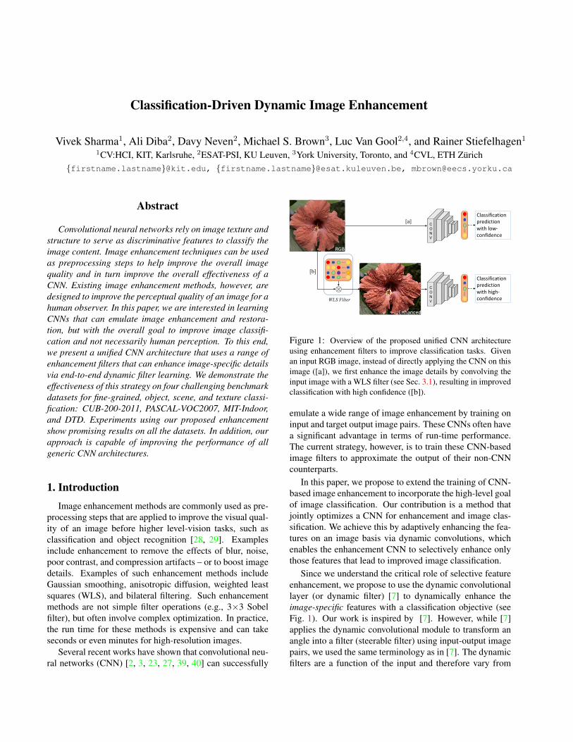
Figure 2: Dynamic enhancement filters. Input to the network are input-output image pairs, as well as image class labels for training. Inthis architecture, we learn a single enhancement filter for each enhancement method individually. The model operates on the luminancecomponent of RGB color space. The enhancement network (i.e., filter-generating network) generates dynamic filter parameters that aresample-specific and conditioned on the input of the enhancement network, with the overall goal to improve image classification. The figurein the upper-right corner shows the whole pipeline workflow.

3. Proposed Method

As previously mentioned, our aim is to learn a dynamicimage enhancement network with the overall goal to im-prove classification, and not necessarily approximating theenhancement methods specifically. To this end, we proposethree CNN architectures described in this section.

Our first architecture is proposed to learn a single en-hancement filter for each enhancement method in an end-to-end fashion (Sec. 3.1) and by end-to-end we mean eachimage will be enhanced and recognized in one unique deepnetwork with dynamic filters. Our second architecture usespre-learned enhancement filters from the first architectureand combines them in a weighted way in the CNN. There isno adaptation of weights of the filters (Sec. 3.2). In our thirdarchitecture, we show end-to-end joint learning of multipleenhancement filters (Sec. 3.3). We also combine them in aweighted way in the CNN. All these setups are jointly opti-mized with a classification objective to selectively enhancethe image feature quality for improved classification. In thenetwork training, image-level class labels are used, whilefor testing the input image can have multiple labels.

3.1. Dynamic Enhancement Filters

In this section we describe our model to learn representa-tive enhancement filters for different enhancement methodsfrom input and target output enhanced image pairs in theend-to-end learning approach with a goal to improve classi-fication performance. Given an input RGB image I , we firsttransform it into the luminance-chrominance Y CbCr colorspace. Our enhancement method operates on the luminancecomponent [14] of the RGB image. This allows our filterto modify the overall tonal properties and sharpness of theimage without affecting the color. The luminance imageY ∈ Rh×w is then convolved with an image enhancementmethod E : Y → T , resulting in an enhanced target outputluminance image T ∈ Rh×w, where h, and w denote theheight and width in the input Y respectively. We generate

target images for a range of enhancement methods E as apreprocessing step (see Section. 4.2 for more details). Forfilter generation, we explicitly use a dataset of only one en-hancement method at a time for learning the transformation.The scheme is illustrated in Figure 2.

First stage (enhancement stage): The enhancementnetwork (EnhanceNet) is inspired by [7, 18, 20], and iscomposed of convolutional and fully-connected layers. TheEnhanceNet maps the input to the filter. The enhancementnetwork takes the one channel luminance image Y and out-puts filters fΘ, Θ ∈ Rs×s×n, where Θ is the parameters ofthe transformation generated dynamically by the enhance-ment network, s is the filter size, and n is the number offilters, being equal to 1 for a single generated filter meantfor one channel luminance image. The generated filter isapplied to the input image Y (i, j) at every spatial position(i,j) to output predicted image Y

′(i, j) = fΘ(Y (i, j)) with

Y′ ∈ Rh×w. The filters are image-specific, and are condi-

tioned on Y . For generating the enhancement filter param-eters Θ, the network is trained using mean squared error(MSE) between the target image T and the network’s pre-dicted output image Y

′. Note that, the parameters of the

filter are obtained as the output of a EnhanceNet that mapsthe input to a filter and therefore vary from one sample toanother. To compare the reconstruction image Y

′with the

ideal T , we use MSE loss as a measure of image quality, al-though we note that more complex loss functions could beused [10].

The chrominance component is then recombined, andthe image is transformed back into RGB, I

′. We found that

the filters learned the expected transformation and appliedthe correct enhancement to the image. Figure 5 shows qual-itative results with dynamically enhanced image textures.

Second stage (classification stage): The predicted out-put image I

′from Stage 1 is fed as an input to the classifica-

tion network (ClassNet). As the classification network (e.g.,Alexnet [21]) has fully-connected layers between the lastconvolutional layer and the classification layer, the param-

eters of the fully-connected layer and C-way classificationlayer are learned when fine-tuning a pre-trained network.

End-to-end learning: The Stage 1-2 cascade with twoloss functions - MSE (enhancement) and softmax-loss L(classification) - enables joint optimization by end-to-endpropagation of gradients in both ClassNet and EnhanceNetusing SGD optimizer. The total loss function of the wholepipeline is given by:

LossFilters = MSE(T, Y′) + L(P,y)

Pq =exp(aq)∑Cr=1 exp(ar)

,L(P,y) = −C∑

q=1

yqlog(Pq)(1)

where a is the output of the last fully-connected layer ofClassNet that is fed to a C-way softmax function, y is thevector of true labels for image I , and C is the number ofclasses.

We fine-tune the whole pipeline until convergence, thusleading to learned enhancement filters in the dynamic en-hancement layer. The joint optimization allows the loss gra-dients from the ClassNet to also back-propagate through theEnhanceNet, making the filter parameters also optimizedfor classification.

3.2. Static Filters for Classification

Here, we show how to integrate the pre-learned enhance-ment filters obtained from the first approach. For each im-age in the train set, we obtain a dynamic filter using our firstapproach. The static filter is computed by taking a meanof all these dynamic filters. The extracted static filters areconvolved with the input luminance Y component of theRGB image I , and the chrominance component is addedand then the image is transformed back to RGB I

′, which is

then fed into the classification network. Figure 3 shows theschematic layout of the whole architecture.

First stage (enhancement stage): We begin by ex-tracting the pre-trained filters for K image enhancementmethods learned from the first approach. Given an in-put luminance image Y , these fΘ,k filters are convolvedwith the input image to generate Y

′

k enhanced images asY

′

k = fΘ,k(Y ), k ∈ K. We also include an identity fil-ter (K+1) to generate the original image, as some learnedenhancements may perform worse than the original imageitself. We then investigate two different strategies to weightWk the enhancement methods: (1) giving equal weightswith value equal to 1/K, and (2) giving weights on the basisof MSE, as discussed in Sec. 3.3.

The output of this stage is a set of enhanced luminanceimages and their corresponding weights indicating the po-tential importance for pushing to the next stage of the clas-sification pipeline. Chrominance is then recombined, andthe images are transformed back to RGB, I

′

k.

Second stage (classification stage): The enhanced im-ages I

′

k for K image enhancement methods and original im-age are fed as an input to the classification network one byone sequentially, with class labels and their weights Wk in-dicating the importance of the enhancement method for theinput image. Similar to the last approach, the network pa-rameters of the fully-connected layer and C-way classifica-tion layer are fine-tuned using a pre-trained network in anend-to-end learning approach.

End-to-end training: The loss of the network trainingis the weighted Wk sum of the individual softmax losses Lk

term. The weighted loss is given as:

LossStat =

K+1∑k=1

WkLk(P,y) (2)

where W is the weight indicating the importance of the Kenhancement method, where WK+1 = 1 for original RGBimage, contributing to the total loss of the whole pipeline.

3.3. Multiple Dynamic Filters for Classification

Here, we recycle the architectures from Sections 3.1-3.2.Figure 4 shows the schematic layout of the whole architec-ture. Our architecture uses the similar architecture proposedin Sec. 3.1; we dynamically generate K filters using K en-hancement networks, one for each enhancement method. Inthis proposed architecture, the loss associated with Stage 1is the MSE between the predicted output images Y

′

k and thetarget output images Tk.

For computing the weights of each enhancement method,the MSE for the enhanced images are transformed toweights Wk by comparing their relative strengths as:Wk = MSEk/

∑Km=1 MSEm, followed by Wk =

(Wk −max(W ))/(min(W ) −max(W )). Since now themin(W ) is zero, in order to avoid giving zero-weight toone of the enhancement methods, we subtract the second-min(W )/2 from W and add the second-min(W ) to theWk with min(W ). Finally, we scale the weights Wk =

Wk/∑K

m=1 Wm with the constraint that the sum of theweights for all K methods should be equal to 1. The en-hanced images with the smallest errors obtain the highestweight, and vice versa. In addition, we also compare againstgiving equal weights to all enhancement methods. Of bothweighting strategies, MSE-based weighting yielded the bestresults, and was therefore selected as the default. Note thatwe also include the original image by simply convolvingit with an identity filter (K+1) similar to approach 2: theweight for the RGB image is set to 1, i.e. WK+1 = 1. Dur-ing training, the weights are estimated by cross-validationon the train/validation set, while for the testing phase, weuse these pre-computed weights. Further, we observed thattraining the network without regularization of weights hasprevented the model from converging throughout the learn-

WLS Filter

Shared Weights

Weight, ()

Stage 2

Weight, (*.)

WeightedLoss

CONV

Classification Network

Stage 1

Scene

Identity Filter

$+%

Input RGB Image

& Luminance Image

Y

Chrominance Image

'-%

CbCr

',.-%

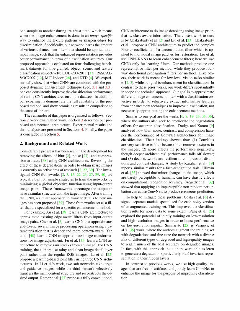
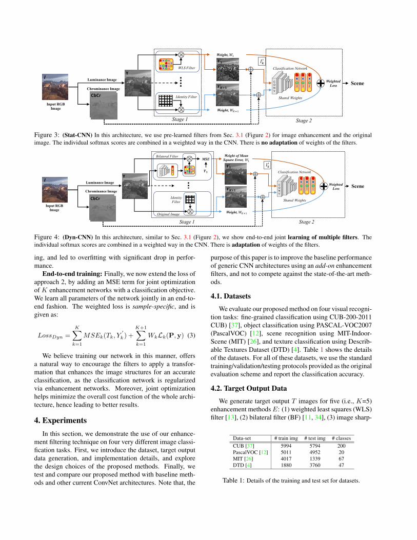
Figure 3: (Stat-CNN) In this architecture, we use pre-learned filters from Sec. 3.1 (Figure 2) for image enhancement and the originalimage. The individual softmax scores are combined in a weighted way in the CNN. There is no adaptation of weights of the filters.

Shared Weights

Stage 2

Weighted Loss

CONV

Classification Network

Stage 1

Scene

$+%Bilateral Filter

CONV

"-

MSE

Input RGB Image

$ Luminance Image

Chrominance Image

CbCr

Weight, (*.)

',.-%

Weight of Mean Square Error, ()

'-%

& Y

Identity Filter

Original Image

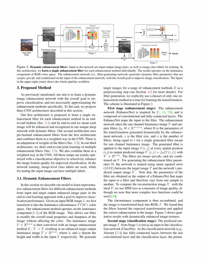
Figure 4: (Dyn-CNN) In this architecture, similar to Sec. 3.1 (Figure 2), we show end-to-end joint learning of multiple filters. Theindividual softmax scores are combined in a weighted way in the CNN. There is adaptation of weights of the filters.

ing, and led to overfitting with significant drop in perfor-mance.

End-to-end training: Finally, we now extend the loss ofapproach 2, by adding an MSE term for joint optimizationof K enhancement networks with a classification objective.We learn all parameters of the network jointly in an end-to-end fashion. The weighted loss is sample-specific, and isgiven as:

LossDyn =

K∑k=1

MSEk(Tk, Y′

k ) +

K+1∑k=1

WkLk(P,y) (3)

We believe training our network in this manner, offersa natural way to encourage the filters to apply a transfor-mation that enhances the image structures for an accurateclassification, as the classification network is regularizedvia enhancement networks. Moreover, joint optimizationhelps minimize the overall cost function of the whole archi-tecture, hence leading to better results.

4. ExperimentsIn this section, we demonstrate the use of our enhance-

ment filtering technique on four very different image classi-fication tasks. First, we introduce the dataset, target outputdata generation, and implementation details, and explorethe design choices of the proposed methods. Finally, wetest and compare our proposed method with baseline meth-ods and other current ConvNet architectures. Note that, the

purpose of this paper is to improve the baseline performanceof generic CNN architectures using an add-on enhancementfilters, and not to compete against the state-of-the-art meth-ods.

4.1. Datasets

We evaluate our proposed method on four visual recogni-tion tasks: fine-grained classification using CUB-200-2011CUB) [37], object classification using PASCAL-VOC2007(PascalVOC) [12], scene recognition using MIT-Indoor-Scene (MIT) [26], and texture classification using Describ-able Textures Dataset (DTD) [4]. Table 1 shows the detailsof the datasets. For all of these datasets, we use the standardtraining/validation/testing protocols provided as the originalevaluation scheme and report the classification accuracy.

4.2. Target Output Data

We generate target output T images for five (i.e., K=5)enhancement methods E: (1) weighted least squares (WLS)filter [13], (2) bilateral filter (BF) [11, 34], (3) image sharp-

Data-set # train img # test img # classesCUB [37] 5994 5794 200PascalVOC [12] 5011 4952 20MIT [26] 4017 1339 67DTD [4] 1880 3760 47

Table 1: Details of the training and test set for datasets.

ening filter (Imsharp), (4) guided filter (GF) [16], and (5)histogram equalization (HistEq). Given an input image,we first transform the RGB color space into a luminance-chrominance color space, and then apply these enhance-ment methods on the luminance image to obtain an en-hanced luminance image. This enhanced luminance imageis then used as the target image for training. We used defaultparameters for WLS and Imsharp, and for BF, GF and His-tEq parameters are adapted to each image, thus requiring noparameter setting. For comprehensive discussion, we referthe readers to [11, 13, 16]. The source code for fast BF [11],WLS [13] is publicly available, and others are available inthe Matlab framework.

4.3. Implementation Details

We use the MatCovNet and Torch frameworks, and allthe ConvNets are trained on a TitanX GPU. Here we dis-cuss the implementation details for ConvNet training (1)with dynamic enhancement filter networks, (2) with staticenhancement filters, and (3) without enhancement filters asa classic ConvNet training scenario.

We evaluate our design on AlexNet [21],GoogleNet [31], VGG-VD [30], VGG-16 [30], andBN-Inception [17]. In each case, the models are pre-trained on the ImageNet [8] and then fine-tuned on thetarget datasets. To fine-tune the network, we replace the1000-way classification layer with a C-way softmax layer,where C is the number of classes in the target dataset. Forfine-tuning the different architectures depending on thedataset about 60-90 epochs (batch size 32) were used, witha scheduled learning rate decrease, starting with a smalllearning rate 0.01. All ConvNet architectures are trainedwith identical optimization schemes, using SGD optimizerwith a fixed weight decay of 5 × 10−4 and a scheduledlearning rate decrease. We follow two steps to fine-tune thewhole network. First, we fine-tune (last two fc layers) theConvNet architecture using RGB images, and then embedit in Stat/Dyn-CNN for fine-tuning the whole network withenhancement filters, by setting a small learning rate forall layers except the last two fc layers, which have a highlearning rate. Specifically, for example, in BN-Inceptionthe network requires a fixed input size of 224 × 224. Theimages are mean-subtracted before network training. Weapply data augmentation [21, 30] by cropping the fourcorners, center, and their x-axis flips, along with colorjittering (and the cropping procedure repeated for each ofthese) for network training. Ahead we provide more detailsfor ConvNet training using BN-Inception.−Dynamic enhancement filters (Dyn-CNN): The en-

hancement network consists of ∼570k learnable model pa-rameters, with the last fully-connected layer (i.e., dynamicfilter parameters) containing 36 neurons - that is, filter-size6 × 6. We initialize the enhancement networks’ model pa-

rameters randomly, except for the last fully-connected layer,which is initialized to regress the identity transform (zeroweights, and identity transform bias), suggested in [18]. Weinitialize the learning rate with 0.01 and decrease it by afactor of 10 after every 15k iterations. The maximum num-ber of iterations is set to 90k. In terms of computationspeed, the training enhancement network along with BN-Inception takes approx. 7% more training time for networkconvergence in comparison to BN-Inception for approach1 (Sec. 3.1). We use five enhancement networks for gen-erating five enhancement filters (one for each method) forapproach 3 (Sec. 3.3). We also include original RGB imagetoo.−Without enhancement filters (FC-CNN): Similar to

classical ConvNets’ fine-tuning scenario, we replace the lastclassification layer of a pre-trained model with a C-wayclassification layer before fine-tuning. The fully connectedlayers and the classification layer are fine-tuned. We initial-ize the learning rate with 0.01 and decrease it by a factorof 10 after every 15k iterations. The maximum number ofiterations is set to 45k.−Static enhancement filters (Stat-CNN): Similar to

FC-CNN, here, we have five enhanced images for five staticfilters and original RGB image as the sixth input that arefed as input to the ConvNets for network training. In prac-tice, the static filters for image enhancement are very low-complex operations. The optimization scheme used here isthe same as FC-CNN. We use all the five static learned fil-ters for approach 2 (Sec. 3.2).Testing: As previously mentioned, the input RGB imageis transformed into luminance-chrominance color space,and then the luminance image is convolved with the en-hancement filter, leading to an enhanced luminance im-age. Chrominance is then recombined to the enhanced lu-minance image and the image is transformed back to RGB.For ConvNet testing, an input frame with either be an RGBimage or an enhanced RGB image using the static or dy-namic filters is fed into the network. In total, five enhancedimages (one for each filter) and the original RGB image arefed into the network, sequentially. For final image label pre-diction, the predictions of all images are combined througha weighted sum, where the pre-computed weights W areobtained from Dyn-CNN.

4.4. Fine-Grained Classification

In this section, we use CUB-200-2011 [37] dataset asa test bed to explore the design choices of our proposedmethod, and then finally compare our method with baselinemethods and the current methods.Dataset: CUB [37] is a fine-grained bird species classifi-cation dataset. The dataset contains 20 bird species with11,788 images. For this dataset, we measure the accuracyof predicting a class for an image.

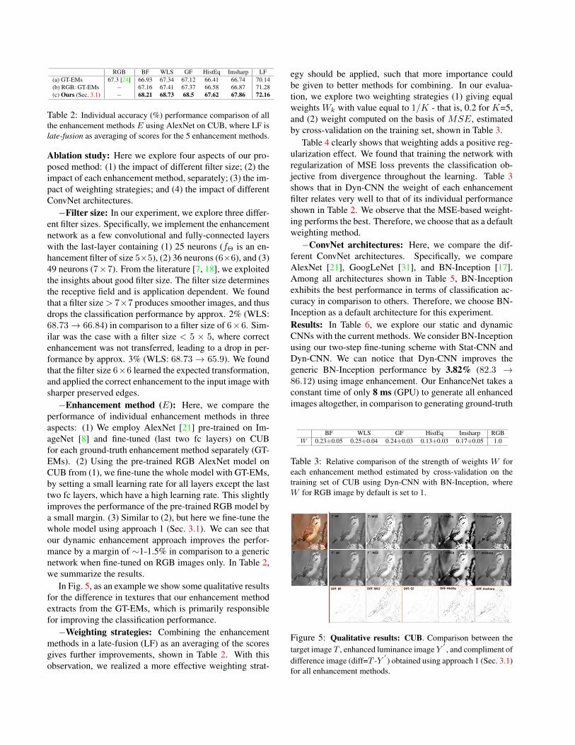
RGB BF WLS GF HistEq Imsharp LF(a) GT-EMs 67.3 [24] 66.93 67.34 67.12 66.41 66.74 70.14(b) RGB: GT-EMs − 67.16 67.41 67.37 66.58 66.87 71.28(c) Ours (Sec. 3.1) − 68.21 68.73 68.5 67.62 67.86 72.16

Table 2: Individual accuracy (%) performance comparison of allthe enhancement methods E using AlexNet on CUB, where LF islate-fusion as averaging of scores for the 5 enhancement methods.

Ablation study: Here we explore four aspects of our pro-posed method: (1) the impact of different filter size; (2) theimpact of each enhancement method, separately; (3) the im-pact of weighting strategies; and (4) the impact of differentConvNet architectures.−Filter size: In our experiment, we explore three differ-

ent filter sizes. Specifically, we implement the enhancementnetwork as a few convolutional and fully-connected layerswith the last-layer containing (1) 25 neurons (fΘ is an en-hancement filter of size 5×5), (2) 36 neurons (6×6), and (3)49 neurons (7×7). From the literature [7, 18], we exploitedthe insights about good filter size. The filter size determinesthe receptive field and is application dependent. We foundthat a filter size > 7×7 produces smoother images, and thusdrops the classification performance by approx. 2% (WLS:68.73→ 66.84) in comparison to a filter size of 6×6. Sim-ilar was the case with a filter size < 5 × 5, where correctenhancement was not transferred, leading to a drop in per-formance by approx. 3% (WLS: 68.73→ 65.9). We foundthat the filter size 6×6 learned the expected transformation,and applied the correct enhancement to the input image withsharper preserved edges.−Enhancement method (E): Here, we compare the

performance of individual enhancement methods in threeaspects: (1) We employ AlexNet [21] pre-trained on Im-ageNet [8] and fine-tuned (last two fc layers) on CUBfor each ground-truth enhancement method separately (GT-EMs). (2) Using the pre-trained RGB AlexNet model onCUB from (1), we fine-tune the whole model with GT-EMs,by setting a small learning rate for all layers except the lasttwo fc layers, which have a high learning rate. This slightlyimproves the performance of the pre-trained RGB model bya small margin. (3) Similar to (2), but here we fine-tune thewhole model using approach 1 (Sec. 3.1). We can see thatour dynamic enhancement approach improves the perfor-mance by a margin of ∼1-1.5% in comparison to a genericnetwork when fine-tuned on RGB images only. In Table 2,we summarize the results.

In Fig. 5, as an example we show some qualitative resultsfor the difference in textures that our enhancement methodextracts from the GT-EMs, which is primarily responsiblefor improving the classification performance.−Weighting strategies: Combining the enhancement

methods in a late-fusion (LF) as an averaging of the scoresgives further improvements, shown in Table 2. With thisobservation, we realized a more effective weighting strat-

egy should be applied, such that more importance couldbe given to better methods for combining. In our evalua-tion, we explore two weighting strategies (1) giving equalweights Wk with value equal to 1/K - that is, 0.2 for K=5,and (2) weight computed on the basis of MSE, estimatedby cross-validation on the training set, shown in Table 3.

Table 4 clearly shows that weighting adds a positive reg-ularization effect. We found that training the network withregularization of MSE loss prevents the classification ob-jective from divergence throughout the learning. Table 3shows that in Dyn-CNN the weight of each enhancementfilter relates very well to that of its individual performanceshown in Table 2. We observe that the MSE-based weight-ing performs the best. Therefore, we choose that as a defaultweighting method.−ConvNet architectures: Here, we compare the dif-

ferent ConvNet architectures. Specifically, we compareAlexNet [21], GoogLeNet [31], and BN-Inception [17].Among all architectures shown in Table 5, BN-Inceptionexhibits the best performance in terms of classification ac-curacy in comparison to others. Therefore, we choose BN-Inception as a default architecture for this experiment.Results: In Table 6, we explore our static and dynamicCNNs with the current methods. We consider BN-Inceptionusing our two-step fine-tuning scheme with Stat-CNN andDyn-CNN. We can notice that Dyn-CNN improves thegeneric BN-Inception performance by 3.82% (82.3 →86.12) using image enhancement. Our EnhanceNet takes aconstant time of only 8 ms (GPU) to generate all enhancedimages altogether, in comparison to generating ground-truth

BF WLS GF HistEq Imsharp RGBW 0.23±0.05 0.25±0.04 0.24±0.03 0.13±0.03 0.17±0.05 1.0

Table 3: Relative comparison of the strength of weights W foreach enhancement method estimated by cross-validation on thetraining set of CUB using Dyn-CNN with BN-Inception, whereW for RGB image by default is set to 1.

𝑻:WLS 𝑻:GF 𝑻:HistEq 𝑻:Imsharp

𝒀

𝑻:BF𝑰

𝒀$:WLS 𝒀$: GF 𝒀$: HistEq 𝒀$: Imsharp𝒀$:BF

Diff:WLS Diff: GF Diff:HistEq Diff: ImsharpDiff:BF

Figure 5: Qualitative results: CUB. Comparison between thetarget image T , enhanced luminance image Y

′, and compliment of

difference image (diff=T -Y′) obtained using approach 1 (Sec. 3.1)

for all enhancement methods.

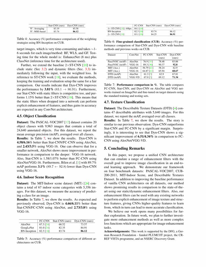
Stat-CNN (ours) Dyn-CNN (ours)W : Averaging 83.19 85.58W : MSE-based 83.74 86.12

Table 4: Accuracy (%) performance comparison of the weightingstrategies using BN-Inception on CUB.

target images, which is very time-consuming and takes ∼1-6 seconds for each image/method: BF, WLS, and GF. Test-ing time for the whole model is: EnhanceNet (8 ms) plusClassNet (inference time for the architecture used).

Further, we extend the baseline 2×ST-CNN [18] to in-clude static (Sec 3.2) and dynamic filters (Sec. 3.3) im-mediately following the input, with the weighted loss. Inreference to ST-CNN work [18], we evaluate the methods,keeping the training and evaluation setup the same for a faircomparison. Our results indicate that Dyn-CNN improvesthe performance by 3.81% (83.1 → 86.91). Furthermore,our Stat-CNN with static filters is competitive too, and per-forms 1.15% better than 2×ST-CNN [18]. This means thatthe static filters when dropped into a network can performexplicit enhancement of features, and thus gains in accuracyare expected in any ConvNet architecture.

4.5. Object Classification

Dataset: The PASCAL-VOC2007 [12] dataset contains 20object classes with 9,963 images that contain a total of24,640 annotated objects. For this dataset, we report themean average precision (mAP), averaged over all classes.Results: In Table 7, we show the results. Dyn-CNN is4.58/6.16% better than Stat-CNN/FC-CNN using AlexNet,and 2.43/3.5% using VGG-16. One can observe that for asmaller network, AlexNet shows more improvement in per-formance in comparison to the deeper: VGG-16 network.Also, Stat-CNN is 1.58/1.07% better than FC-CNN usingAlexNet/VGG-16. Furthermore, Bilen et al. [1] with 89.7%mAP performs 3.1% (89.7 ← 92.8) lower than Dyn-CNNusing VGG-16.

4.6. Indoor Scene Recognition

Dataset: The MIT-Indoor scene dataset (MIT) [26] con-tains a total of 67 indoor scene categories with 5,356 im-ages. For this dataset, we measure the accuracy of predict-ing a class for an image.Results: In Table 7, we show the results. As expected andpreviously observed, Dyn-CNN is 4.66/6.11% better thanStat-CNN/FC-CNN using AlexNet, and 2.73/3.8% usingVGG-16.

FC-CNN Stat-CNN (ours) Dyn-CNN (ours)AlexNet 67.3 [24] 68.52 73.57GoogLeNet 81.0 [24] 82.35 84.91BN-Inception 82.3 [18] 83.74 86.12

Table 5: Accuracy (%) performance comparison of different ar-chitectures on CUB.

FC-CNN Stat-CNN (ours) Dyn-CNN (ours)4× ST-CNN [18]: 448px 84.1 [18] − −BN-Inception 82.3 [18] 83.74 86.122× ST-CNN [18] 83.1 [18] 84.25 86.91

Table 6: Fine-grained classification (CUB). Accuracy (%) per-formance comparison of Stat-CNN and Dyn-CNN with baselinemethods and previous works on CUB.

Dataset ConvNet FC-CNN Stat-CNN Dyn-CNN(ours) (ours)

PasclVOC (mAP) AlexNet 76.9 [33] 78.48 83.06PasclVOC (mAP) VGG-16 89.3 [30] 90.37 92.8MIT (Acc.) AlexNet 56.79 [41] 58.24 62.9MIT (Acc.) VGG-16 64.87 [41] 65.94 68.67DTD (mAP) AlexNet 61.3 [5] 62.9 67.81DTD (mAP) VGG-VD 67.0 [5] 69.12 71.34

Table 7: Performance comparison in %. The table comparesFC-CNN, Stat-CNN, and Dyn-CNN on AlexNet and VGG net-works trained on ImageNet and fine-tuned on target datasets usingthe standard training and testing sets.

4.7. Texture Classification

Dataset: The Describable Texture Datasets (DTD) [4] con-tains 47 describable attributes with 5,640 images. For thisdataset, we report the mAP, averaged over all classes.Results: In Table 7, we show the results. The story issimilar to our previous observation: Dyn-CNN outperformsStat-CNN and FC-CNN by a significant margin. Surpris-ingly, it is interesting to see that Dyn-CNN shows a sig-nificant improvement of 6.51/4.34% in comparison to FC-CNN using AlexNet/VGG-VD.

5. Concluding RemarksIn this paper, we propose a unified CNN architecture

that can emulate a range of enhancement filters with theoverall goal to improve image classification in an end-to-end learning approach. We demonstrate our frameworkon four benchmark datasets: PASCAL-VOC2007, CUB-200-2011, MIT-Indoor Scene, and Describable TexturesDataset. In addition to improving the baseline performanceof vanilla CNN architectures on all datasets, our methodshows promising results in comparison to the state-of-the-art using our static/dynamic enhancement filters. Also, ourenhancement filters can be used with any existing networksto perform explicit enhancement of image texture and struc-ture features, giving CNNs higher-quality features to learnfrom, which in turn can lead to more accurate classification.

We believe our work opens many possibilities for fur-ther exploration. In future work, we plan to further investi-gate more enhancement methods as well as more complexloss functions which are appropriate for image enhancementtasks.Acknowledgements: This work is supported by the DFG, a Ger-man Research Foundation - funded PLUMCOT project, the CR-REF VISTA programme, and an NSERC Discovery Grant.

References[1] H. Bilen and A. Vedaldi. Weakly supervised deep detection

networks. In CVPR, 2016.[2] A. Chakrabarti. A neural approach to blind motion deblur-

ring. In ECCV, 2016.[3] Q. Chen, J. Xu, and V. Koltun. Fast image processing with

fully-convolutional networks. In ICCV, 2017.[4] M. Cimpoi, S. Maji, I. Kokkinos, S. Mohamed, and

A. Vedaldi. Describing textures in the wild. In CVPR, 2014.[5] M. Cimpoi, S. Maji, I. Kokkinos, and A. Vedaldi. Deep filter

banks for texture recognition, description, and segmentation.IJCV, 2016.

[6] G. B. P. da Costa, W. A. Contato, T. S. Nazare, J. E. Neto, andM. Ponti. An empirical study on the effects of different typesof noise in image classification tasks. arxiv:1609.02781,2016.

[7] B. De Brabandere, X. Jia, T. Tuytelaars, and L. Van Gool.Dynamic filter networks. In NIPS, 2016.

[8] J. Deng, W. Dong, R. Socher, L.-J. Li, K. Li, and L. Fei-Fei. Imagenet: A large-scale hierarchical image database. InCVPR, 2009.

[9] S. Dodge and L. Karam. Understanding how image qualityaffects deep neural networks. In QoMEX, 2016.

[10] A. Dosovitskiy and T. Brox. Generating images with per-ceptual similarity metrics based on deep networks. In NIPS,2016.

[11] F. Durand and J. Dorsey. Fast bilateral filtering for the dis-play of high-dynamic-range images. In ACM TOG, 2002.

[12] M. Everingham, A. Zisserman, C. K. Williams, L. Van Gool,M. Allan, C. M. Bishop, O. Chapelle, N. Dalal, T. Deselaers,G. Dorko, et al. The pascal visual object classes challenge2007 (voc2007) results. 2007.

[13] Z. Farbman, R. Fattal, D. Lischinski, and R. Szeliski. Edge-preserving decompositions for multi-scale tone and detailmanipulation. In ACM TOG, 2008.

[14] C. Fredembach and S. Susstrunk. Colouring the near-infrared. In CIC, 2008.

[15] X. Fu, J. Huang, X. Ding, Y. Liao, and J. Paisley. Clearingthe skies: A deep network architecture for single-image rainremoval. arxiv:1609.02087, 2016.

[16] K. He, J. Sun, and X. Tang. Guided image filtering. In ECCV,2010.

[17] S. Ioffe and C. Szegedy. Batch normalization: Acceleratingdeep network training by reducing internal covariate shift.arXiv:1502.03167, 2015.

[18] M. Jaderberg, K. Simonyan, A. Zisserman, et al. Spatialtransformer networks. In NIPS, 2015.

[19] S. Karahan, M. K. Yildirum, K. Kirtac, F. S. Rende, G. Bu-tun, and H. K. Ekenel. How image degradations affect deepcnn-based face recognition? In BIOSIG, 2016.

[20] B. Klein, L. Wolf, and Y. Afek. A dynamic convolutionallayer for short range weather prediction. In CVPR, 2015.

[21] A. Krizhevsky, I. Sutskever, and G. E. Hinton. Imagenetclassification with deep convolutional neural networks. InNIPS, 2012.

[22] Y. Li, J.-B. Huang, N. Ahuja, and M.-H. Yang. Deep jointimage filtering. In ECCV, 2016.

[23] S. Liu, J. Pan, and M.-H. Yang. Learning recursive filtersfor low-level vision via a hybrid neural network. In ECCV,2016.

[24] K. Matzen and N. Snavely. Bubblenet: Foveated imaging forvisual discovery. In ICCV, pages 1931–1939, 2015.

[25] X. Peng, J. Hoffman, X. Y. Stella, and K. Saenko. Fine-to-coarse knowledge transfer for low-res image classification.In ICIP, 2016.

[26] A. Quattoni and A. Torralba. Recognizing indoor scenes. InCVPR, 2009.

[27] T. Remez, O. Litany, R. Giryes, and A. M. Bronstein. Deepclass aware denoising. arxiv:1701.01698, 2017.

[28] V. Sharma, J. Y. Hardeberg, and S. George. Rgb-nir imageenhancement by fusing bilateral and weighted least squaresfilters. Journal of Imaging Science and Technology, 2017.

[29] V. Sharma and L. Van Gool. Does v-nir based imageenhancement come with better features? arXiv preprintarXiv:1608.06521, 2016.

[30] K. Simonyan and A. Zisserman. Very deep convolutionalnetworks for large-scale image recognition. In ICLR, 2015.

[31] C. Szegedy, W. Liu, Y. Jia, P. Sermanet, S. Reed,D. Anguelov, D. Erhan, V. Vanhoucke, and A. Rabinovich.Going deeper with convolutions. In CVPR, 2015.

[32] C. Szegedy, W. Zaremba, I. Sutskever, J. Bruna, D. Erhan,I. Goodfellow, and R. Fergus. Intriguing properties of neuralnetworks. arxiv:1312.6199, 2013.

[33] P. Tang, X. Wang, B. Shi, X. Bai, W. Liu, and Z. Tu. Deepfishernet for object classification. arxiv:1608.00182, 2016.

[34] C. Tomasi and R. Manduchi. Bilateral filtering for gray andcolor images. In ICCV, 1998.

[35] S. Ullman, L. Assif, E. Fetaya, and D. Harari. Atomsof recognition in human and computer vision. NationalAcademy of Sciences, 2016.

[36] I. Vasiljevic, A. Chakrabarti, and G. Shakhnarovich. Exam-ining the impact of blur on recognition by convolutional net-works. arxiv:1611.05760, 2016.

[37] C. Wah, S. Branson, P. Welinder, P. Perona, and S. Belongie.The caltech-ucsd birds-200-2011 dataset. 2011.

[38] L. Xu, J. S. Ren, C. Liu, and J. Jia. Deep convolutional neuralnetwork for image deconvolution. In NIPS, 2014.

[39] L. Xu, J. S. Ren, Q. Yan, R. Liao, and J. Jia. Deep edge-aware filters. In ICML, 2015.

[40] Z. Yan, H. Zhang, B. Wang, S. Paris, and Y. Yu. Automaticphoto adjustment using deep neural networks. ACM TOG,2016.

[41] B. Zhou, A. Khosla, A. Lapedriza, A. Torralba, and A. Oliva.Places: An image database for deep scene understanding.arxiv:1610.02055, 2016.